Multiparametric bifurcations for a model in epidemiology

J. Math. Biol. (1996) 35: 21—36

Multiparametric bifurcations for a model inepidemiology

Marcos Lizana, Jesus Rivero

Department of Mathematics, Faculty of Sciences, Universidad de Los Andes, Merida 5101,Venezuela. E-mail: [email protected]

Received 8 April 1994; received in revised form 29 June 1995

Abstract. In the present paper we make a bifurcation analysis of an SIRSepidemiological model depending on all parameters. In particular we areinterested in codimension-2 bifurcations.

Key words: Epidemiological model — Homoclinic orbit — Periodic trajectories

1 Introduction

Liu in [7, p. 6] points out that the dynamical behavior of epidemics is usuallyvery complicated and many infectious diseases exhibit recurrent outbreaks inlarge populations. In this respect Liu introduced and examined in [7] a quitegeneral SEIRS epidemiological model. The SEIRS model involves a new classof population, i.e., the exposed but not yet infectious class (E) in addition tosusceptible (S), infectious (I) and recovered (R) classes. In this work we willconcentrate on an SIRS epidemiological model examined in detail in Liu et al.in [6]. The SIRS model can be regarded as the limiting case of the SEIRSmodel when the average latent periods tends to zero, see [7, p. 42]. Theyassumed that the mathematical model describing this phenomenon is given bythe following system of ordinary differential equations:

S@"!IH(I, S)!bS#cR#B (N)

I@"IH(I, S)!(b#v)I (1.1)

R@"vI!(b#c)R

where S — susceptible, I — infective, R — removed or recovered; H(I, S) is theincidence rate per infective individual; b is the per capita death rate; B (N) isthe (non-negative) birth rate (a function of N"S#I#R); v is the per capitarecovery rate; and c is the per capita rate of loss of immunity. We assume thatall newborn individuals are susceptible, and that all coefficients are positive.

The functions B (N) and H(I, S) are assumed to be differentiable; further,for all I, H (I, 0)"0 and LH/LS'0. The latter condition reflects the biolo-gically intuitive requirement that the incidence rate be an increasing functionof the number of susceptibles. In this model, the traditional assumption thatthe incidence rate is proportional to the product of the numbers of infectivesand susceptibles is dropped; and they also introduce births, deaths, and loss ofimmunity. The possible mechanism leading to nonlinear incidence rates arediscussed in [7]. In this framework, the system (1.1) can exhibit qualitativelydifferent dynamical behaviors, including Hopf bifurcations, saddle-node bifur-cations, and homoclinic loop bifurcations. They remark that these may beimportant epidemiologically in that they demonstrate the possibility of infec-tion outbreak and collapse, or autonomous periodic coexistence of diseaseand host. Investigating the behavior of the system (1.1) on the planeS#I#R"N

0, and assuming that the incidence rate is of the form kIpSq,

where k, p, and q are positive constants, Liu et al. gave in [6] a detailedanalysis of the bifurcation of the codimension one. The constant N

0represents

population equilibrium in the absence of the disease. In the special case p"2,q"1, numerical studies made in [6] indicated the existence of homoclinicsolutions for a range of values of each of the parameters involved in (1.1).Derrick and van den Driessche in [3] for an SIRS disease transmission modelin a nonconstant population, using numerical techniques, also showed theexistence of homoclinic solutions. No proofs were provided in either of theabove mentioned papers.

In the present paper, we make a bifurcation analysis of the model depend-ing on all the parameters. In particular we are interested in codimension-2bifurcations that occur in a two dimensional parameter region. Following [5],we use singular changes of coordinates in order to transform (1.1) intoa two-parameter family of ODE, where the new parameters are related to thetrace (k), and the determinant (l) of certain system linearized at a suitableequilibrium. We show that for each small l90, there is a locally unique k (l)for which the system (1.1) has a homoclinic orbit. Furthermore, there areparameter values for which there are periodic trajectories and other values forwhich (1.1) has a trajectory joining the critical point.

2 The general model and analysis

In this section, we summarize the main facts obtained in [7, chapter 2] relatedto system (1.1), that we need in the sequel.

Summing the three equations in (1.1), we obtain

N@"B (N)!bN . (2.1)

We assume that (2.1) admits a positive stable equilibrium in the absence of thedisease. This assumption is not a serious restriction because, for (2.1), everysolution must tend either to a positive equilibrium or to extinction, or mustincrease without bound. For any biologically reasonable model, the latter

22 M. Lizana, J. Rivero

situation must be excluded. Thus, unless there exists some nonzero equilib-rium N

0, the population cannot sustain itself even without the disease. Fol-

lowing [6], we will investigate the behavior of the system (1.1) in the planeS#I#R"N

0'0. There, the system can be reduced to the 2-dimensional

system

S@"!I (H, S)!(b#c)S!cI#N0(b#c) ,

(2.2)I@"IH(I, S)!(b#v)I .

The following result holds.

Lemma 1 ¸et X"M(I, S): I70, S70, I#S6N0N. ¹hen, X is positive

invariant under the flow induced by (2.2).

Since X is a compact set, from Lemma 1, it follows that any solution of system(2.2) with initial conditions in X is defined for every t'0.

It is much easier to work with equations that have been scaled todimensionless variables and parameters. Thus, we take

¹"(b#v)t, a"b#cb#v

, a*"1

b#v,

b"c

b#v, IM (¹ )"I(t), SM (¹ )"S(t) .

With this scaling (2.2) becomes

dIMd¹

"a*IM H (IM , SM )!IM ,

(2.3)dSMd¹

"!a*IM H(IM , SM )!aSM !bIM#aN0

.

Hereafter, we assume these transformations have been made and drop thebars over the I and S.

The system (2.3) has a trivial equilibrium (I0, S

0)"(0, N

0) and any non-

trivial equilibrium in this system is given implicitly by

a*H(I, S)"1, !I!aS!bI#aN0"0 ,

or

a*HAI, N0!

1#ba

IB"1 . (2.4)

The stability of such non-trivial equilibrium depends on the eigenvalues ofthe matrix

M"Ca*I

LH

LI

!1!a*ILH

LI!b

a*ILH

LS

!a*ILH

LS!aD

Multiparametric bifurcations for a model in epidemiology 23

evaluated at the equilibrium. If the parameters of this model are changed sothat the trace of M passes from negative to positive while the determinantremains positive, a Hopf bifurcation occurs; if suitable higher order conditionsare satisfied, this bifurcation may transform a stable equilibrium into a stableperiodic solution. Since LH/LS'0, a necessary condition for this to happen isthat LH/LI'0 (see [7, Prop. 2.1.1, pp. 12—14]). That is, the dependence of theincidence rate IH on I must be greater than the one of a linear function.

Such a model also may admit a saddle-node bifurcation, at which twonon-trivial equilibria (a saddle and a node) coalesce and obliterate each other.This bifurcation is determined by the joint solution of (2.4) and the tangencycondition

LH

LI"

1#ba

LH

LS.

Substituting this condition into the determinant of the matrixM, we see thatdetM"0 at a saddle-node bifurcation.

3 The incidence rate H (I, S)"kIp~1Sq

In this section, we examine the case H (I, S)"kIp~1Sq, where k, p and q arepositive constants. The system (2.3) now becomes

I@"cIpSq!1 ,(3.1)

S@"!cIpSq!aS!bI#aN0

,

where c"a*k. We know from the previous section that a necessary conditionfor Hopf bifurcation is LH/LI'0, which implies that p'1. The only equilib-ria of (3.1) are the trivial stable node (0, N

0), which is ignored throughout the

paper, and the intersection points of the two curves

S"1

qJcIp~1, S"N

0!

1#ba

I .

Depending on the parameters, there exist two, one or no such equilibria(I0, S

0).

Since, we are interested in codimension-2 bifurcations which occur ina two dimensional parameter region, hereafter we will fix the parameters c, b,p, q in the system (3.1). This selection of the parameters is motivated bybiological considerations. In [6], the changes in the dynamical behavior of theflow are related to N

0. The possibility of choosing others pairs as bifurcation

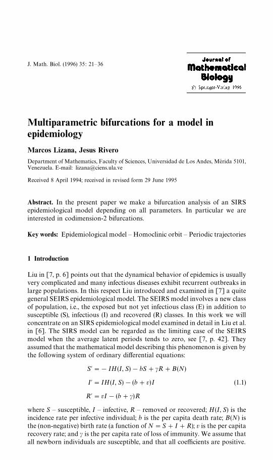
parameters can be studied in an analogous manner. Thus, the dependence ofthe equilibria on the parameters is best characterized by identifying theseequilibria with the points of a two-dimensional manifold M in (a, I

0, N

0)-

space, defined by the equation

!

1#ba

I0#N

0"(c)~

1q (I0

)1~pq , (3.2)


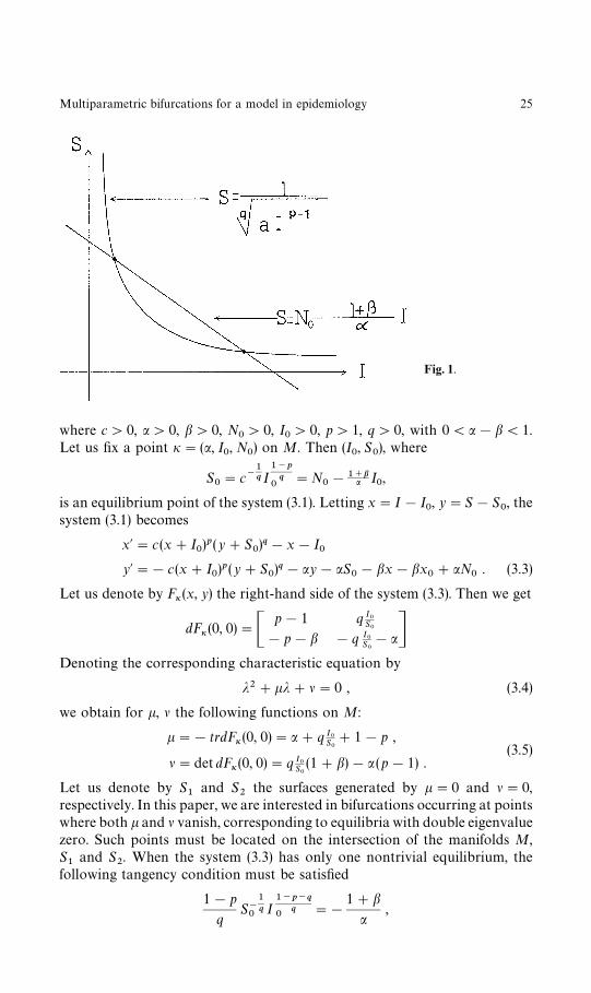
Fig. 1.

where c'0, a'0, b'0, N0'0, I

0'0, p'1, q'0, with 0(a!b(1.

Let us fix a point i"(a, I0, N

0) on M. Then (I

0, S

0), where

S0"c~1

q I0

1~pq "N

0!1`ba I

0,

is an equilibrium point of the system (3.1). Letting x"I!I0, y"S!S

0, the

system (3.1) becomes

x@"c(x#I0)p(y#S

0)q!x!I

0y@"!c(x#I

0)p (y#S

0)q!ay!aS

0!bx!bx

0#aN

0. (3.3)

Let us denote by Fi(x, y) the right-hand side of the system (3.3). Then we get

dFi(0, 0)"Cp!1

!p!bq I

0S0

!q I0

S0!aD

Denoting the corresponding characteristic equation by

j2#kj#l"0 , (3.4)

we obtain for k, l the following functions on M:

k"!trdFi(0, 0)"a#q I0

S0#1!p ,

(3.5)l"det dFi(0, 0)"q I

0S0(1#b)!a (p!1) .

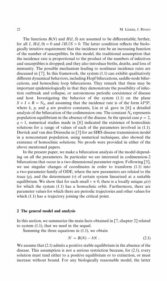
Let us denote by S1

and S2

the surfaces generated by k"0 and l"0,respectively. In this paper, we are interested in bifurcations occurring at pointswhere both k and l vanish, corresponding to equilibria with double eigenvaluezero. Such points must be located on the intersection of the manifolds M,S1

and S2. When the system (3.3) has only one nontrivial equilibrium, the

following tangency condition must be satisfied

1!p

qS0~1q I

01~p~q

q "!

1#ba

,


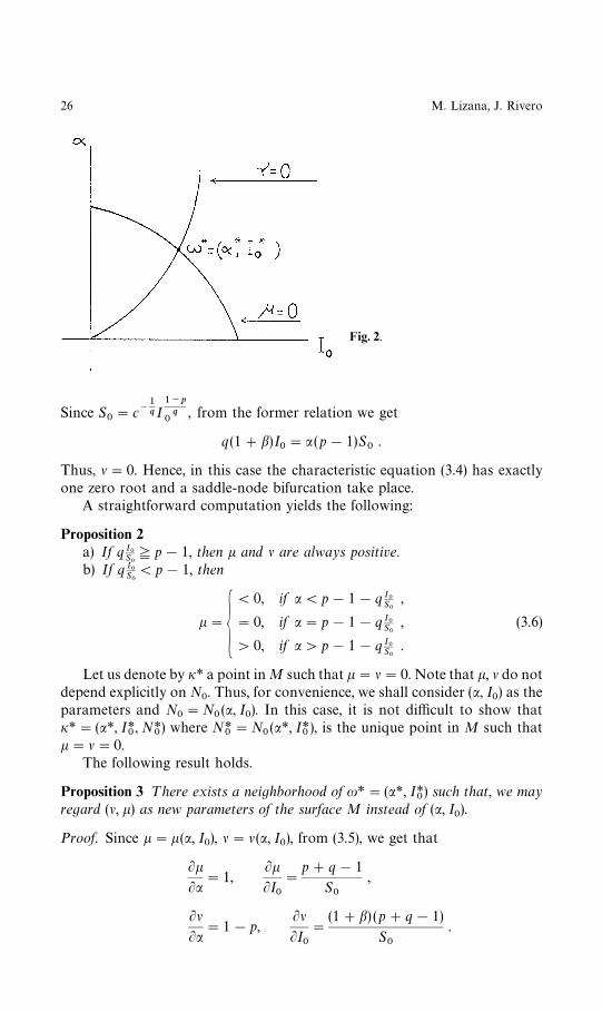
Fig. 2.

Since S0"c~1

qI0

1~pq , from the former relation we get

q (1#b)I0"a (p!1)S

0.

Thus, l"0. Hence, in this case the characteristic equation (3.4) has exactlyone zero root and a saddle-node bifurcation take place.

A straightforward computation yields the following:

Proposition 2a) If q I

0S07p!1, then k and l are always positive.

b) If q I0

S0(p!1, then

k"G(0, if a(p!1!q I

0S0

,

"0, if a"p!1!q I0

S0

,

'0, if a'p!1!q I0

S0

.

(3.6)

Let us denote by i* a point in M such that k"l"0. Note that k, l do notdepend explicitly on N

0. Thus, for convenience, we shall consider (a, I

0) as the

parameters and N0"N

0(a, I

0). In this case, it is not difficult to show that

i*"(a*, I*0, N*

0) where N*

0"N

0(a*, I*

0), is the unique point in M such that

k"l"0.The following result holds.

Proposition 3 ¹here exists a neighborhood of u*"(a*, I*0) such that, we may

regard (l, k) as new parameters of the surface M instead of (a, I0).

Proof. Since k"k(a, I0), l"l(a, I

0), from (3.5), we get that

LkLa

"1,LkLI

0

"

p#q!1

S0

,

LlLa

"1!p,LlLI

0

"

(1#b) (p#q!1)

S0

.


Thus, the Jacobian of the transformation k"k (a, I0), l"l(a, I

0) with respect

to a, I0

is given by

J (a, I0)"

LkLa

LlLI

0

!

LkLI

0

LlLa

"

(p#q!1) (p#b)

S0

,

which it is different from zero for any choice of the parameters in theadmissible region. K

4 Reduction to canonical problems. Unfolding of the bifurcations

As it was already mentioned above, we will consider only neighborhoods ofpoints (a, I

0, N

0) of M satisfying k(a, I

0)"l(a, I

0)"0. From Proposition 2, it

is not difficult to deduce that such point exist if and only if

0(qI0

S0

(

(p!1)2

p. (4.1)

Therefore, in addition to the requirements stated in Sect. 2, we assumeinequality (4.1) throughout the rest of the paper. Then the unique point ofM yielding k"l"0 is given by i*"(a*, I*

0, N*

0). By exploiting k"0, we get

q I*0

S*0"p!1!a*, where S*

0"N*

0!1`ba* I*

0. Then,

dFi*(0, 0)"Cp!1

!p!bp!1!a*

1!p D .

It is easy to check that det dFi*(0, 0)"0, tr dFi*(0, 0)"0.We are studying a planar system with both eigenvalues zero near the

equilibrium point. In order to carry out the investigation of the behavior ofthe flow, we have to consider the quadratic terms of the right-hand side of thesystem (3.3). Expanding the vector field in a power series around the point(x, y)"(0, 0), we get

x@"(p!1)x#qI0

S0

y#Ax2#Bxy#Cy2#· · ·

(4.2)

y@"!(p#b)x!Aa#qI0

S0By!Ax2!Bxy!Cy2#· · ·

where

A"

p(p!1)

2I0

, B"

pq

S0

, C"

q(q!1)

2

I0

S20

.

Now we consider parameters a, I0

such that u"(a, I0) defines a point

i"(a, I0, N

0) on the surface M which is sufficiently close to i*"(a*, I*

0, N*

0).

We shall make two nonsingular changes of variables before rescaling thesystem (4.2). The first is a l, k dependent transformation on x and y designedto put dFi (0, 0) into the form ( 0

~l 1~k). The next change of variables is in the

parameter space alone. We let k"k(a, I0) and l"l (a, I

0). By Proposition 3,


this change of variables is also nonsingular. More precisely, making theparameter dependent affine transformation

xN "x ,

yN "(p!1)x#qI0

S0

y ,

and expressing a and I0

as a function of k and l up to the first order terms, wesee that the system (4.2) becomes

xN @"yN #A1xN 2#B

1xN yN #C

1yN 2#Q

1(xN , yN , l, k)

(4.3)yN @"!lxN !kyN #A

1a*xN 2#B

1a*xN yN #C

1a*yN 2#Q

2(xN , yN , l, k)

where

A1"

(p!1) (1!p!q)

2qI*0

(0 ,

B1"

p!1#q

qI*0

'0 ,

C1"

q!1

2qI*0

.

The terms Qiare power series in (xN , yN , l, k) with powers xN iyN ikllm satisfying

i#j#l#m73 and i#j72, and coefficients depending analytically on(l, k). The linearization of system (4.3) at the point (xN , yN , l, k)"(0, 0, 0, 0) is(0 10 0

). In what follows, we have to investigate (4.3) in a neighborhood of thispoint, which corresponds to i*3M. The method of investigation is to scalevariables in such a way as to blow up the neighborhood of the equilibriumpoint in order to see the fine structure of the flow. We know that A

1(0.

Hence, for k90, l90, we may rescale (4.3) in the following way:

e"k~1 Kl

a*A1K1@2

, xN "e2x1, yN "e3J!a*A

1x2

,

(4.4)q"eJ!a*A

1t, k"eJ!a*A

1q* ,

where k is a new parameter with, say, 0(k61. Then (4.3) becomes

xR1"x

2#e

A1

J!a*A1

x21#eq

1(x

1, x

2, e, q*)

(4.5)

xR2"!k2 (sgn l)x

1!r*x

2!x2

1#e

B1a*

J!a*A1

x1x2#eq

2(x

1, x

2, e, q*)

The terms qiare analytic in all variables, at least of second order with respect

to (x1, x

2), and at least of first order with respect to (e, q*). Such systems have

been treated in the literature, for instance, see [5, 1]. In order to establish thestandard situation we transform (x

1, x

2) into (u, v) in such a way that the two


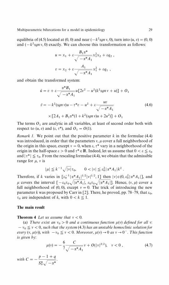
equilibria of (4.5) located at (0, 0) and near (!k2sgn l, 0), turn into (u, v)"(0, 0)and (!k2sgn l, 0) exactly. We can choose this transformation as follows:

u"x1#e

B1a*

J!a*A1

x21x2#eq

2,

v"x2#e

A1

J!a*A1

x21#eq

1,

and obtain the transformed system:

uR "v#ea*B

1J!a*A

1

u[2v2!u2(k2sgn l#u)]#O1

vR"!k2 (sgn l)u!q*v!u2#euv

J!a*A1

(4.6)

][2A1#B

1a*(1#k2(sgn l)u#2u2)]#O

1

The terms O1

are analytic in all variables, at least of second order both withrespect to (u, v) and (e, q*), and O

1"O(1).

Remark 1. We point out that the positive parameter k in the formulae (4.4)was introduced, in order that the parameters l, k cover a full neighborhood ofthe origin in this space, except l"0, when e, q* vary in a neighborhood of theorigin in the half-space e'0 and q*3R. Indeed, let us assume that 0(e6e

0and D q* D6q

0. From the rescaling formulae (4.4), we obtain that the admissible

range for k, l is

DkD6k~1JDlD q0, 0(Dl D6e2

0D a*A

1Dk2 .

Therefore, if k varies in [e~10

D a*A1D1@2 DlD1@2, 1] then DlD3(0, e2

0D a*A

1D], and

k covers the interval [!e0q0JDa*A

1D, e

0q0JDa*A

1D]. Hence, (l, k) cover a

full neighborhood of (0, 0), except l"0. The trick of introducing the newparameter k was proposed by Carr in [2]. There, he proved, pp. 78—79, that e

0,

q0

are independent of k, with 0(k61.

The main result

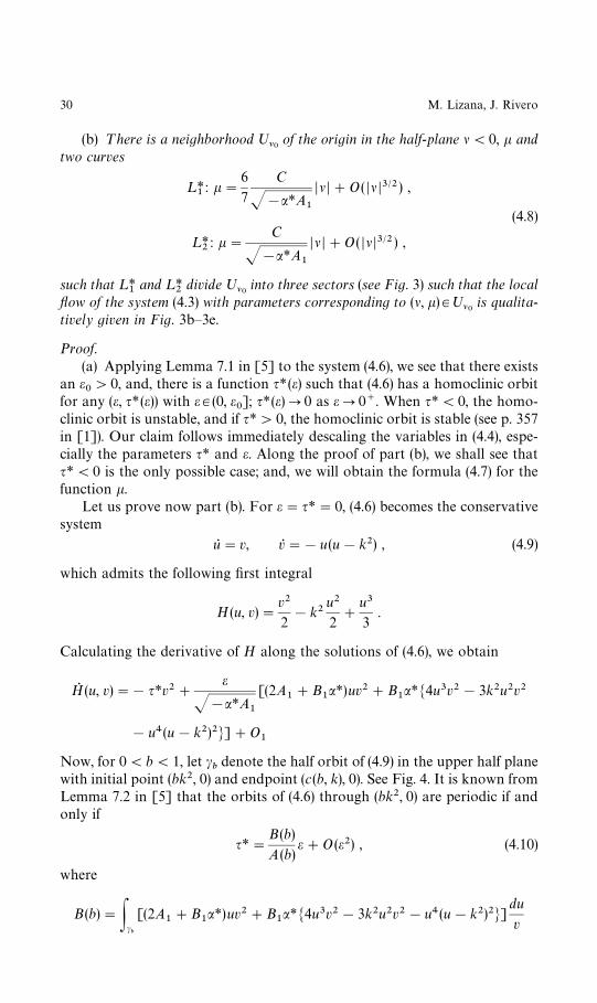
Theorem 4 ¸et us assume that l(0.(a) ¹here exist an l

0'0 and a continuous function k (l) defined for all l:

!l06l(0, such that the system (4.3) has an unstable homoclinic solution for

every (l, k (l)), with !l06l(0. Moreover, k (l)P0 as lP0~. ¹his function

is given by:

k (l)"!

6

7

C

J!a*A1

l#O( DlD3@2 ), l(0 , (4.7)

with C"!

p!1#q

S*0J!a*

.


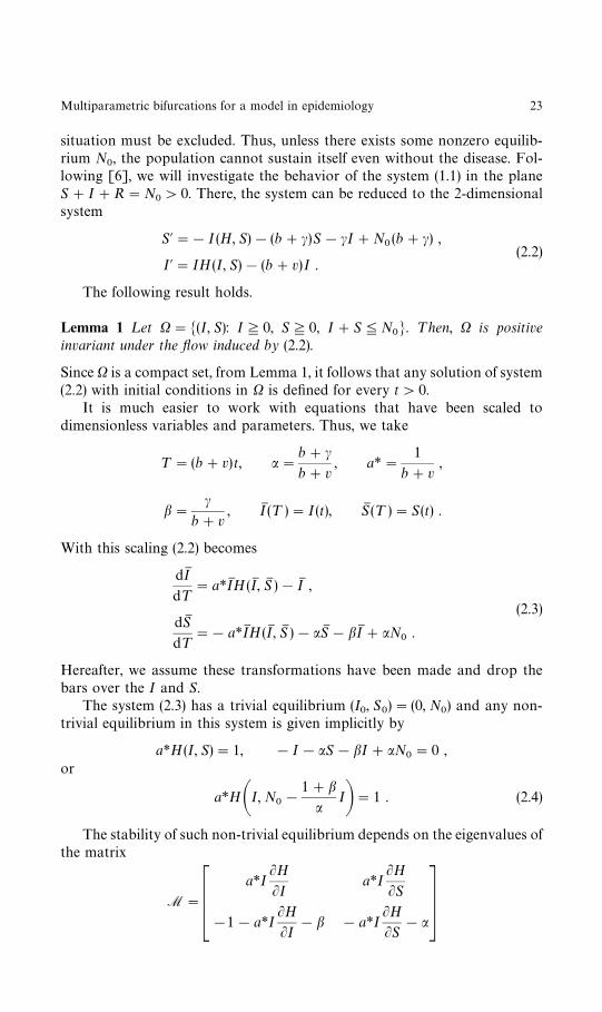
(b) ¹here is a neighborhood ºlÒof the origin in the half-plane l(0, k and

two curves

¸*1: k"

6

7

C

J!a*A1

DlD#O( Dl D3@2) ,

(4.8)

¸*2: k"

C

J!a*A1

DlD#O( DlD3@2 ) ,

such that ¸*1

and ¸*2

divide ºlÒinto three sectors (see Fig. 3) such that the local

flow of the system (4.3) with parameters corresponding to (l, k)3ºlÒis qualita-

tively given in Fig. 3b—3e.

Proof.(a) Applying Lemma 7.1 in [5] to the system (4.6), we see that there exists

an e0'0, and, there is a function q* (e) such that (4.6) has a homoclinic orbit

for any (e, q* (e)) with e3(0, e0]; q*(e)P0 as eP0`. When q*(0, the homo-

clinic orbit is unstable, and if q*'0, the homoclinic orbit is stable (see p. 357in [1]). Our claim follows immediately descaling the variables in (4.4), espe-cially the parameters q* and e. Along the proof of part (b), we shall see thatq*(0 is the only possible case; and, we will obtain the formula (4.7) for thefunction k.

Let us prove now part (b). For e"q*"0, (4.6) becomes the conservativesystem

uR "v, vR"!u(u!k2) , (4.9)

which admits the following first integral

H (u, v)"v2

2!k2

u2

2#

u3

3.

Calculating the derivative of H along the solutions of (4.6), we obtain

HQ (u, v)"!q*v2#e

J!a*A1

[(2A1#B

1a*)uv2#B

1a*M4u3v2!3k2u2v2

!u4(u!k2)2N]#O1

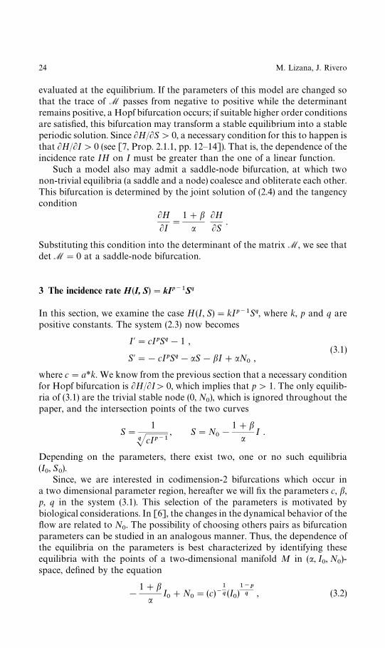
Now, for 0(b(1, let cbdenote the half orbit of (4.9) in the upper half plane

with initial point (bk2, 0) and endpoint (c(b, k), 0). See Fig. 4. It is known fromLemma 7.2 in [5] that the orbits of (4.6) through (bk2, 0) are periodic if andonly if

q*"B (b)

A (b)e#O(e2) , (4.10)

where

B (b)"Pcb

[(2A1#B

1a*)uv2#B

1a*M4u3v2!3k2u2v2!u4 (u!k2)2N]

du

v


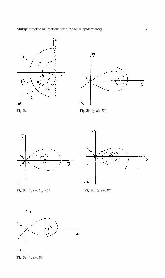
Fig. 3a. Fig. 3b. (c, k)3D*1

Fig. 3c. (c, k)3ºcÒW¸*

1Fig. 3d. (c, k)3D*

2

Fig. 3e. (c, k)3D*3


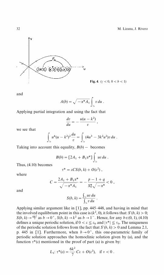
Fig. 4. (c(0, 0(b(1)

and

A(b)"J!a*A1 Pc

b

v du .

Applying partial integration and using the fact that

dv

du"!

u (u!k2)

v,

we see that

Pcb

u4(u!k2)2du

v"Pc

b

(4u3!3k2u2)v du .

Taking into account this equality, B(b)! becomes

B (b)"[2A1#B

1a*] Pc

b

uv du .

Thus, (4.10) becomesq*"eCS(b, k)#O(e2) ,

where

C"

2A1#B

1a*

J!a*A1

"!

p!1#q

S*0J!a*

(0 ,

and

S (b, k)":c

buv du

:cbv du

.

Applying similar argument like in [1], pp. 445—448, and having in mind thatthe involved equilibrium point in this case is (k2, 0), it follows that: S@(b, k)'0;S(b, k)P6kÈ

7as bP0`, S (b, k)Pk2 as bP1~. Hence, for any b3(0, 1), (4.10)

defines a unique periodic solution, if 0(e6e0

and Dq* D6q0. The uniqueness

of the periodic solution follows from the fact that S@(b, k)'0 and Lemma 2.1,p. 445 in [1]. Furthermore, when bP0`, this one-parametric family ofperiodic solution approaches the homoclinic solution given by (a), and thefunction q* (e) mentioned in the proof of part (a) is given by:

¸1: q*(e)"

6k2

7Ce#O(e2), if l(0 .


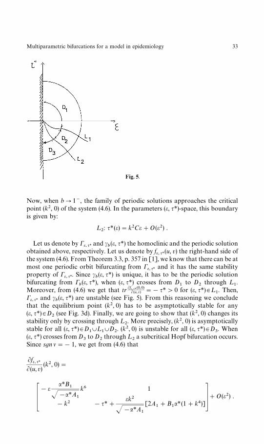
Fig. 5.

Now, when bP1~, the family of periodic solutions approaches the criticalpoint (k2, 0) of the system (4.6). In the parameters (e, q*)-space, this boundaryis given by:

¸2: q*(e)"k2Ce#O (e2) .

Let us denote by Ce, q* and cb(e, q*) the homoclinic and the periodic solution

obtained above, respectively. Let us denote by fe, q*(u, v) the right-hand side ofthe system (4.6). From Theorem 3.3, p. 357 in [1], we know that there can be atmost one periodic orbit bifurcating from Ce, q* and it has the same stabilityproperty of Ce, q*. Since c

b(e, q*) is unique, it has to be the periodic solution

bifurcating from Cb(e, q*), when (e, q*) crosses from D

1to D

2through ¸

1.

Moreover, from (4.6) we get that tr Lfe, q*(0, 0)L(u, v) "!q*'0 for (e, q*)3¸

1. Then,

Ce, q* and cb(e, q*) are unstable (see Fig. 5). From this reasoning we conclude

that the equilibrium point (k2, 0) has to be asymptotically stable for any(e, q*)3D

2(see Fig. 3d). Finally, we are going to show that (k2, 0) changes its

stability only by crossing through ¸2. More precisely, (k2, 0) is asymptotically

stable for all (e, q*)3D1X¸

1XD

2. (k2, 0) is unstable for all (e, q*)3D

3. When

(e, q*) crosses from D3

to D2

through ¸2

a subcritical Hopf bifurcation occurs.Since sgn l"!1, we get from (4.6) that

Lfe, q*L(u, v)

(k2, 0)"

C!e

a*B1

J!a*A1

k6 1

!k2 !q*#ek2

J!a*A1

[2A1#B

1a* (1#k4)]D#O(e2) .


A few computations yield to

a :"trLfe, q*L(u, v)

(k2, 0)"q*!k2Ce#O(e2) ,

b :"detLfe, q*L (u, v)

(k2, 0)"k2#O(e) .

Taking into account that the characteristic equation corresponding to thelinearization of (4.6) around (k2, 0) is j2!aj#b"0 and b'0 for small e,our claim follows immediately from the fact that: a"0 for (e, q*)3¸

2, a'0,

∀ (e, q*)3D3, a(0, ∀ (e, q*)3D

1X¸

1XD

2.

In order to establish our assertions, it is sufficient to descale the param-eters q*, e and the variables x

1, x

2. Indeed, taking into account the Remark 1

and descaling (4.4), we deduce that ¸1

and ¸2

in the (l, k)-space become¸*1

and ¸*2, respectively. Which are given by the relations (4.8). K

Remark 2. In order to establish part (b) of the above theorem, we basicallyfollowed the main ideas of Lemma 2.1, pp. 445—448 in [1]. But, they cannot beapplied directly to our situation. Because, the introduction of the parameterk in (4.4) modifies many computations that are crucial in to determine thecurves in the (l, k)-plane at which the topological structure of the trajectoriesof the system (4.4) changes.

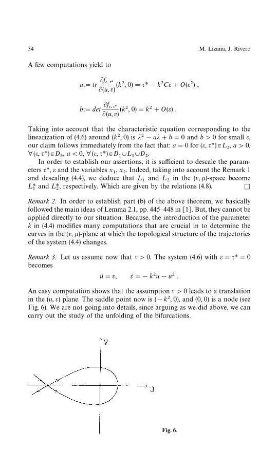
Remark 3. Let us assume now that l'0. The system (4.6) with e"q*"0becomes

uR "v, vR"!k2u!u2 .

An easy computation shows that the assumption l'0 leads to a translationin the (u, v) plane. The saddle point now is (!k2, 0), and (0, 0) is a node (seeFig. 6). We are not going into details, since arguing as we did above, we cancarry out the study of the unfolding of the bifurcations.

Fig. 6.


5 Discussion

The analysis of the bifurcation diagram of Theorem 4 in terms of the originalbiological parameters can be done with the use of formulas (3.5). Indeed,taking into account that

a"b#cb#v

, b"c

b#v, c"a*k"

k

b#v, (5.1)

we can determine M, k, and l as a functions of the original parameters. Fixingk, b, v, p, q, M-becomes a two-dimensional manifold in the three dimensionalspace (c, I

0, N

0). It is not difficult to show that the condition k (c, I

0)"

l(c, I0)"0 leads to the equation

c2#c (2b#v)#(b#v) (b#(p!1)v)"0 . (5.2)

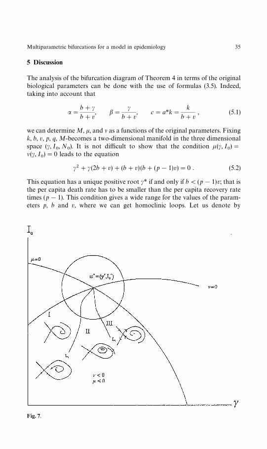
This equation has a unique positive root c* if and only if b((p!1)v; that isthe per capita death rate has to be smaller than the per capita recovery ratetimes (p!1). This condition gives a wide range for the values of the param-eters p, b and v, where we can get homoclinic loops. Let us denote by

Fig. 7.


u*"(c*, I*0) the unique point on M such that k (c*, I*

0)"l (c*, I*

0)"0, the

constant c* is the unique positive root of (5.2) and I*0

is obtained from (3.5)taking into account (5.1) and setting c"c*. Now, for example, an increase ofthe per capita loss of immunity rate of recovered individuals, c, for suitablevalues of the remaining parameters, might eventually give rise to a saddle-node bifurcation (see Fig. 7) which could proceed to the appearance of anunstable homoclinic orbit surrounding the larger endemic equilibrium point(EEP). Thus the homoclinic loop is the separatrix for the epidemiologicalbasins of attraction of the desease free equilibrium and the larger EEP (as theparameters crosses the curve ¸

1of Fig. 7). As c varies driving (k, l) into region

II of Fig. 7, a unique periodic orbit appear and, finally, for values of c driving(k, l) into region III the periodic orbit disappear through a sub-criticalbifurcation.

Acknowledgements. We wish to thank Dr. H.W. Hethcote for introducing us to this model.The first author also like to thank Dr. Jack K. Hale for many useful discussions during thestay at Georgia Tech. Finally, we thank referees for their constructive remarks and fortelling us about the Liu’s PhD thesis.

6 References

1. Chow S.-N., Hale J.: Methods of bifurcation theory. Springer-Verlag (1985)2. Carr J.: Applications of centre manifold theory. Appl. Math. Sc. V. 35. Springer-Verlag

(1981)3. Derrick W. R., van den Driessche P.: A disease transmission model in a non-constant

population. J. Math. Biol. (1993) 31, 495—5124. Hainzl J.: Multiparameter bifurcation of a predator-prey system. SIAM J. Math. Anal.

(1992) 23, 150—1805. Kopell N., Howard L. N.: Bifurcations and trajectories joining critical points. Adv. in

Math. (1975) 18, 306—3586. Liu W., Levin S. A., Iwasa Y.: Influence of nonlinear incidence rates upon the behavior of

SIRS epidemiological models. J. Math. Biol. (1986) 23, 187—2047. Liu W. M: Dynamics of epidemiological models. Recurrent outbreaks in autonomous

systems. PhD thesis. Ithaca: Cornell University 1987

.


Multiparametric bifurcations for a model in epidemiology

Documents