Multinomial Logistic Regression David F. Staples

Welcome message from author
This document is posted to help you gain knowledge. Please leave a comment to let me know what you think about it! Share it to your friends and learn new things together.
Transcript

Multinomial Logistic Regression
David F. Staples
Outline
• Review of Logistic Regression• BCS Example
• Extension to Multiple Response Groups• Nominal Categories• Ordinal Categories
• Model Fitting & Interpretation• Shallow Lake Trophic Status
Logistic Regression
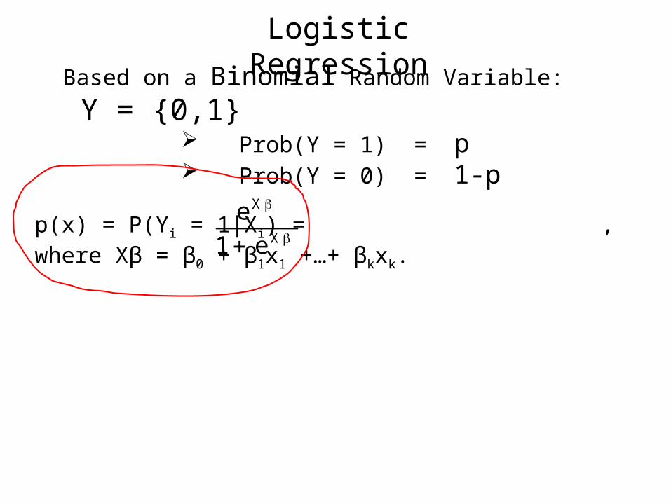
Based on a Binomial Random Variable: Y = {0,1} Prob(Y = 1) = p Prob(Y = 0) = 1-p
p(x) = P(Yi = 1|Xi) = , where Xβ = β0 + β1x1 +…+ βkxk.
X
X
e1
e

Logistic Regression
Based on a Binomial Random Variable: Y = {0,1} Prob(Y = 1) = p Prob(Y = 0) = 1-p
p(x) = P(Yi = 1|Xi) = , where Xβ = β0 + β1x1 +…+ βkxk.
A logit transformation is used to linearize p(x):
= β0 + β1x1 +…+ βkxk = Xβ
p(x)1
p(x)ln)x(g
X
X
e1
e
→ The β’s give the additive effect of X’s on the Log Odds
Log Odds of ‘Success’

Logistic Regression Example
Model p as a function of Macrophyte Patch Area
glm(BCS ~ Patch_area, family = binomial)
Estimate SE z Pr(>|z|) Intercept -2.433e+00 5.108e-01 -4.764 1.9e-06 Patch_area 1.765e-04 4.725e-05 3.736 0.0001
Dichotomous Variable is the Presence/Absence of BCS
Y = 1 if BCS Present
Y = 0 if BCS Absent
p = Prob(BCS Present)

Interpreting Logistic Regression
glm(BCS ~ Patch_area, family = binomial)
Estimate SE z Pr(>|z|) Intercept -2.433e+00 5.108e-01 -4.764 1.9e-06 Patch_area 1.765e-04 4.725e-05 3.736 0.0001
Effect of Patch Area on P(BCS)• Non-Linear Transformation Value of Intercept Value of Other Variables

Interpreting Logistic Regression
For the average size patch area (8374), the log odds ratio would be:
-2.433 + 0.0001765 * 8374 = -0.955
exponentiate to get the Odds of Success:
exp(-.955) = p/1-p = 0.38,
Solve for p,
Prob(BCS Present|Area=8374) = .28
glm(BCS ~ Patch_area, family = binomial)
Estimate SE z Pr(>|z|) Intercept -2.433e+00 5.108e-01 -4.764 1.9e-06 Patch_area 1.765e-04 4.725e-05 3.736 0.0001

Interpreting Logistic Regression
When p = 0.5, the log odds equals 0,
–2.433 + .0001765*Area = 0.
Thus, the patch area for p = .50 is
2.433/.0001765 = 13784.7
glm(BCS ~ Patch_area, family = binomial)
Estimate SE z Pr(>|z|) Intercept -2.433e+00 5.108e-01 -4.764 1.9e-06 Patch_area 1.765e-04 4.725e-05 3.736 0.0001
p1
pODDS

Multinomial Logistic Regression
• Logistic Regression with > 2 response categories• Model Probabilities Relative to ‘Reference’ Category• Response May be Nominal or Ordinal
Nominal Ordinal

Shallow Lake Trophic Status
3 Categories Defining Lake State:Y = 1 if Lake ClearY = 2 if Lake Shifting StatesY = 3 if Lake Turbid

Nominal (un-ordered) Multinomial Logistic
library(nnet)
multinom(StateNom ~ TP)
(Int) TP2 -2.47 0.0123 -1.89 0.014
Std. Errors: (Int) TP2 0.549 0.0043 0.447 0.004
Residual Deviance: 113.8345 AIC: 121.8345

Nominal (un-ordered) Multinomial LogisticLibrary(nnet)
multinom(StateNom ~ TP)
(Int) TP2 -2.47 0.0123 -1.89 0.014
For TP = 50
50*012.47.2)(
)(ln
Clearp
Shiftingp
85.1
16.0)85.1exp(
p(Shifting) is about 16% of p(Clear)

Nominal (un-ordered) Multinomial Logistic
For TP = 50
50*014.89.1)(
)(ln
Clearp
Turbidp
20.1
30.0)20.1exp(
p(Turbid) is about 30% of p(Clear)
Library(nnet)
multinom(StateNom ~ TP)
(Int) TP2 -2.47 0.0123 -1.89 0.014
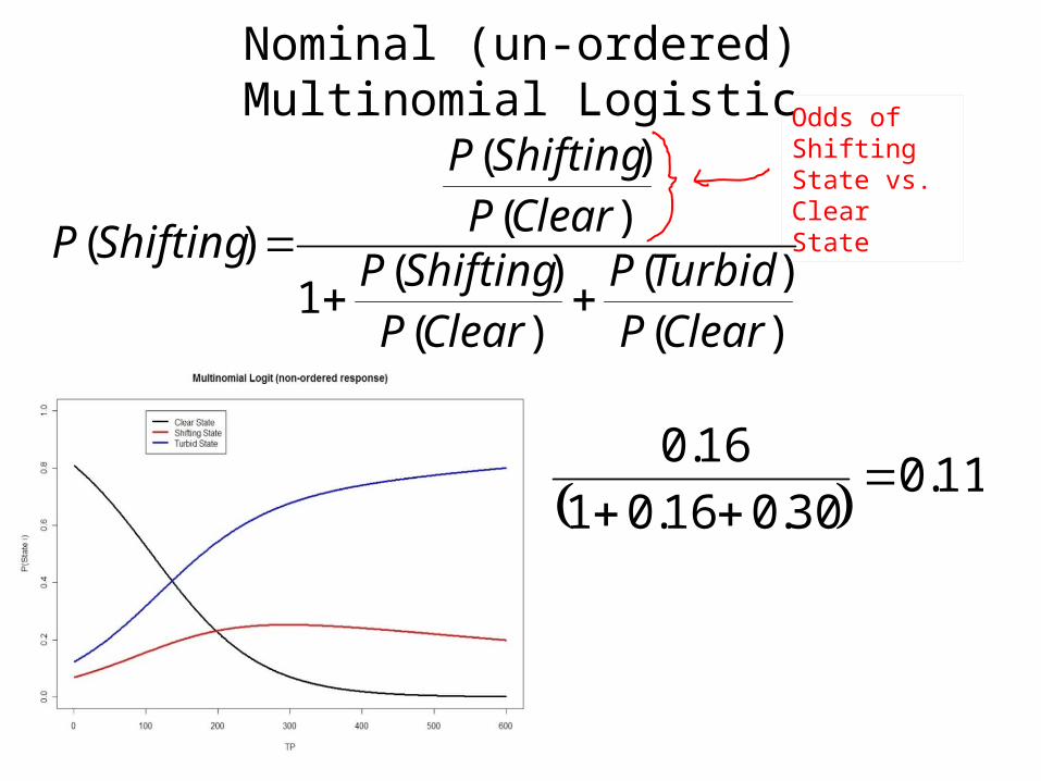
Nominal (un-ordered) Multinomial Logistic
)()(
)()(
1
)()(
)(
ClearPTurbidP
ClearPShiftingP
ClearPShiftingP
ShiftingP
11.030.016.01
16.0
Odds of Shifting State vs. Clear State

Ordinal Multinomial Logistica.k.a. Proportional Odds Model
3 Ordered Status Categories:Y = 1 if lake clearY = 2 if lake shifting statesY = 3 if lake turbid

Ordinal Multinomial Logistica.k.a. Proportional Odds Model
library(MASS)StateOrd = as.ordered(StateNom)
polr(StateOrd ~ TP)
Value SE t valueTP 0.009 0.002 3.81
Intercepts: Value SE t value1|2 1.103 0.342 3.222|3 1.889 0.397 4.76
Residual Deviance: 118.99 AIC: 124.9897
3 Ordered Status Categories:Y = 1 if lake clearY = 2 if lake shifting statesY = 3 if lake turbid
Assume Same Slope => Fewer Parameters

m2 = polr(StateOrd ~ TP)
newd = data.frame(TP = seq(0,600))
prd = predict(m2, newdata=newd, type='p')
matplot(newd$TP,prd)

Nominal/Ordinal Comparison
Nominal (un-ordered) Multinomial Logistic
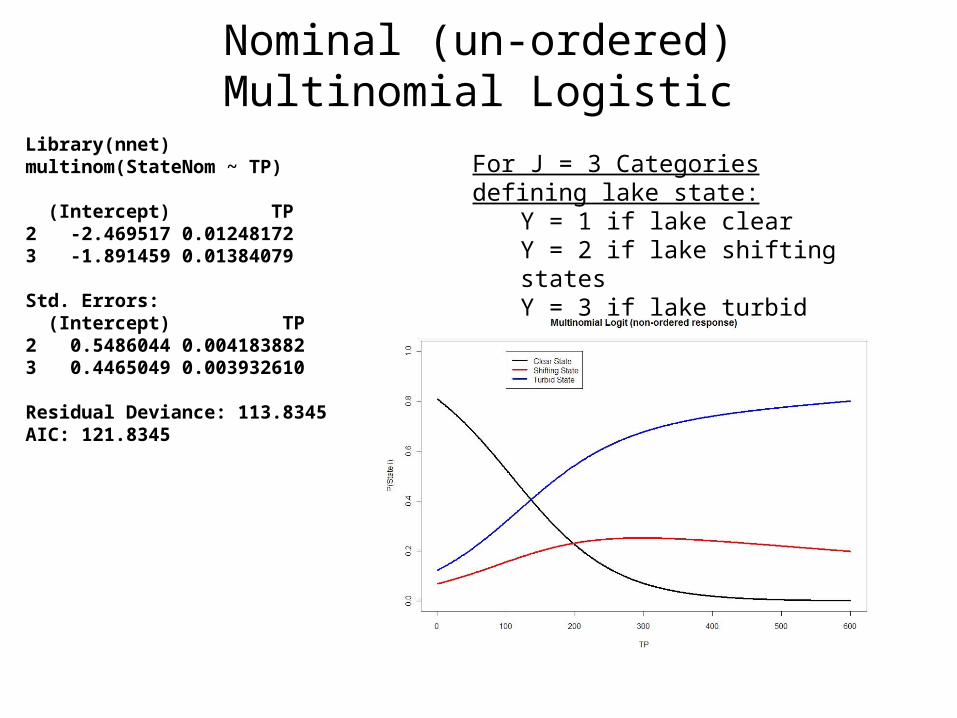
Library(nnet)multinom(StateNom ~ TP)
(Intercept) TP2 -2.469517 0.012481723 -1.891459 0.01384079
Std. Errors: (Intercept) TP2 0.5486044 0.0041838823 0.4465049 0.003932610
Residual Deviance: 113.8345 AIC: 121.8345
For J = 3 Categories defining lake state:Y = 1 if lake clearY = 2 if lake shifting statesY = 3 if lake turbid
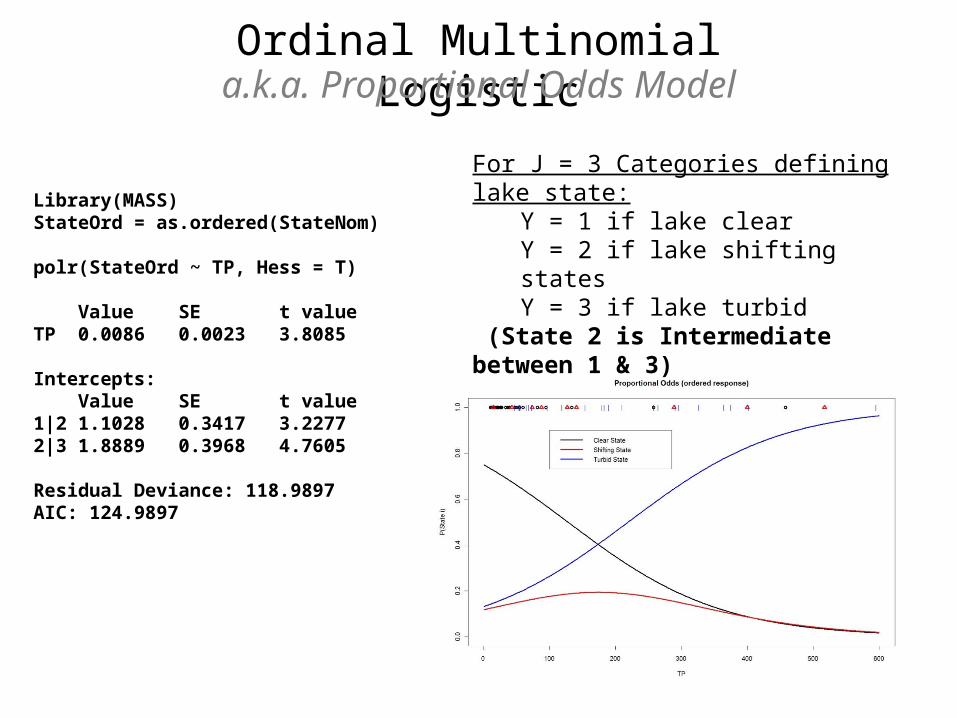
Ordinal Multinomial Logistica.k.a. Proportional Odds Model
For J = 3 Categories defining lake state:Y = 1 if lake clearY = 2 if lake shifting statesY = 3 if lake turbid
(State 2 is Intermediate between 1 & 3)
Library(MASS)StateOrd = as.ordered(StateNom)
polr(StateOrd ~ TP, Hess = T)
Value SE t valueTP 0.0086 0.0023 3.8085
Intercepts: Value SE t value1|2 1.1028 0.3417 3.2277 2|3 1.8889 0.3968 4.7605
Residual Deviance: 118.9897 AIC: 124.9897
Related Documents