MULTINOMIAL LOGISTIC REGRESSION - College of ...

390

26MULTINOMIAL

LOGISTIC REGRESSION

CAROLYN J. ANDERSON

LESLIE RUTKOWSKI

Chapter 24 presented logistic regressionmodels for dichotomous response vari-ables; however, many discrete response

variables have three or more categories (e.g.,political view, candidate voted for in an elec-tion, preferred mode of transportation, orresponse options on survey items). Multicate-gory response variables are found in a widerange of experiments and studies in a variety ofdifferent fields. A detailed example presented inthis chapter uses data from 600 students fromthe High School and Beyond study (Tatsuoka &Lohnes, 1988) to look at the differences amonghigh school students who attended academic,general, or vocational programs. The students’socioeconomic status (ordinal), achievementtest scores (numerical), and type of school(nominal) are all examined as possible explana-tory variables. An example left to the interestedreader using the same data set is to model thestudents’ intended career where the possibilitiesconsist of 15 general job types (e.g., school,manager, clerical, sales, military, service, etc.).Possible explanatory variables include gender,achievement test scores, and other variables inthe data set.

Many of the concepts used in binary logisticregression, such as the interpretation of parame-ters in terms of odds ratios and modeling prob-abilities, carry over to multicategory logisticregression models; however, two major modifica-tions are needed to deal with multiple categoriesof the response variable. One difference is thatwith three or more levels of the response variable,there are multiple ways to dichotomize theresponse variable. If J equals the number of cate-gories of the response variable, then J(J – 1)/2 dif-ferent ways exist to dichotomize the categories.In the High School and Beyond study, the threeprogram types can be dichotomized into pairsof programs (i.e., academic and general, voca-tional and general, and academic and vocational).

How the response variable is dichotomizeddepends, in part, on the nature of the variable. Ifthere is a baseline or control category, then theanalysis could focus on comparing each of theother categories to the baseline. With three ormore categories, whether the response variableis nominal or ordinal is an important consider-ation. Since models for nominal responsescan be applied to both nominal and ordinalresponse variables, the emphasis in this chapter

26-Osborne (Best)-45409.qxd 10/9/2007 5:52 PM Page 390

is on extensions of binary logistic regression tomodels designed for nominal response vari-ables. Furthermore, a solid understanding of themodels for nominal responses facilitates master-ing models for ordinal data. A brief overview ofmodels for ordinal variables is given toward theend of the chapter.

A second modification to extend binarylogistic regression to the polytomous case is theneed for a more complex distribution for theresponse variable. In the binary case, the distri-bution of the response is assumed to be bino-mial; however, with multicategory responses,the natural choice is the multinomial distribu-tion, a special case of which is the binomial dis-tribution. The parameters of the multinomialdistribution are the probabilities of the cate-gories of the response variable.

The baseline logit model, which is sometimesalso called the generalized logit model, is thestarting point for this chapter because it is awell-known model, it is a direct extension ofbinary logistic regression, it can be used withordinal response variables, and it includesexplanatory variables that are attributes of indi-viduals, which is common in the social sciences.The baseline model is a special case of the condi-tional multinomial logit model, which caninclude explanatory variables that are character-istics of the response categories, as well as attri-butes of individuals.

A word of caution is warranted here. In theliterature, the term multinomial logit model some-times refers to the baseline model, and sometimesit refers to the conditional multinomial logitmodel. An additional potential source of confu-sion lies in the fact that the baseline model isa special case of the conditional model, which inturn is a special case of Poisson (log-linear)regression.1 These connections enable researchersto tailor models in useful ways and test interestinghypotheses that could not otherwise be tested.

MULTINOMIAL REGRESSION MODELS

One Explanatory Variable Model

The most natural interpretation of logisticregression models is in terms of odds and oddsratios; therefore, the baseline model is first pre-sented as a model for odds and then presented asa model for probabilities.

ODDS

The baseline model can be viewed as the setof binary logistic regression models fit simulta-neously to all pairs of response categories. Withthree or more categories, a binary logisticregression model is needed for each (nonredun-dant) dichotomy of the categories of the responsevariable. As an example, consider high schoolprogram types from the High School andBeyond data set (Tatsuoka & Lohnes, 1988).There are three possible program types: aca-demic, general, and vocational. Let P(Yi = aca-demic), P(Yi = general), and P(Yi = vocational)be the probabilities of each of the program typesfor individual i. Recall from Chapters 24 and 25that odds equal ratios of probabilities. In ourexample, only two of the three possible pairs ofprogram types are needed because the third canbe found by taking the product of the other two.Choosing the general program as the reference,the odds of academic versus general and theodds of vocational versus general equal

The third odds, academic versus vocational,equals the product of the two odds in (1a) and(1b)—namely,

(2)

More generally, let J equal the number of cate-gories or levels of the response variable. Of the J(J– 1)/2 possible pairs of categories, only (J – 1) ofthem are needed. If the same category is used inthe denominator of the (J – 1) odds, then the setof odds will be nonredundant, and all other pos-sible odds can be formed from this set. In thebaseline model, one response category is chosenas the baseline against which all other responsecategories are compared. When a natural baselineexists, that category is the best choice in terms ofconvenience of interpretation. If there is not anatural baseline, then the choice is arbitrary.

= P(Yi = academic)/P(Yi = general)

P(Yi = vocational)/P(Yi = general).

P(Yi = academic)

P(Yi = vocational)

P(Yi = academic)

P(Yi = general)

P(Yi = vocational)

P(Yi = general).

Multinomial Logistic Regression 391

(1a)

(1b)


392 BEST PRACTICES IN QUANTITATIVE METHODS

As a Model for Odds

Continuing our example from the HighSchool and Beyond data, where the general pro-gram is chosen as the baseline category, the firstmodel contains a single explanatory variable, themean of five achievement test scores for eachstudent (i.e., math, science, reading, writing, andcivics). The baseline model is simply two binarylogistic regression models applied to each pair ofprogram types; that is,

(3)

and

(4)

where P(Yi = academic|xi), P(Yi = general|xi),and P(Yi = vocational|xi) are the probabili-ties for each program type given meanachievement test score xi for student i, theαjs are intercepts, and the βjs are regressioncoefficients. The odds of academic versusvocational are found by taking the ratio of(3) and (4),

(5)

where α3 = (α1 − α2) and β3 = (β1 − β2).For generality, let j = 1, . . . , J represent cate-

gories of the response variable. The numericalvalues of j are just labels for the categories of theresponse variable. The probability that individuali is in category j given a value of xi on the explana-tory variable is represented by P(Yi = j|xi). Takingthe Jth category as the baseline, the model is

(6)

When fitting the baseline model to data,the binary logistic regressions for the (J – 1)odds must be estimated simultaneously toensure that intercepts and coefficients for allother odds equal the differences of the corre-sponding intercepts and coefficients (e.g., α3

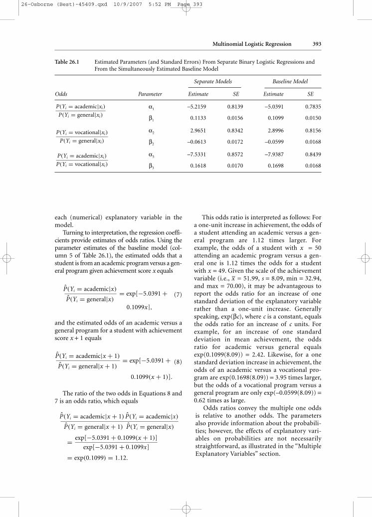
= (α1 − α2) and β3 = (β1 − β2) in Equation 5).To demonstrate this, three separate binarylogistic regression models were fit to the HighSchool and Beyond data, as well as the base-line regression model, which simultaneouslyestimates the models for all the odds. Theestimated parameters and their standarderrors are reported in Table 26.1. Althoughthe parameters for the separate and simulta-neous cases are quite similar, the logical rela-tionships between the parameters when themodels are fit separately are not met (e.g., β̂1

− β̂2= 0.1133 + 0.0163 = 0.1746 ≠ 0.1618);however, the relationships hold for simulta-neous estimation (e.g., β̂1 − β̂2 = 0.1099 +0.0599 = 0.1698).

Besides ensuring that the logical relation-ships between parameters are met, a secondadvantage of simultaneous estimation is that itis a more efficient use of the data, which in turnleads to more powerful statistical hypothesistests and more precise estimates of parameters.Notice that the parameter estimates in Table26.1 from the baseline model have smaller stan-dard errors than those in the estimation ofseparate regressions. When the model is fitsimultaneously, all 600 observations go into theestimation of the parameters; however, in theseparately fit models, only a subset of the obser-vations is used to estimate the parameters (e.g.,453 for academic and general, 455 for academicand vocational, and only 292 for vocational andgeneral).

A third advantage of the simultaneous esti-mation, which is illustrated later in thischapter, is the ability to place equality restric-tions on parameters across odds. For example,if two βs are very similar, they could be forcedto be equal. The complexity of the baselinemodel increases as the number of responseoptions increases, and any means of reducingthe number of parameters that must be inter-preted can be a great savings in terms of inter-preting and summarizing the results. Forexample, if we modeled career choice with 15possible choices, there would be 14 nonredun-dant odds and 14 different βs to interpret forfor j = 1, . . ., (J − 1).

P(Yi = j|xi)

P(Yi = J |xi)= exp[αj + βj xi]

P(Yj = academic|xi)

P(Yj = vocational|xi)= exp[α1 + β1xi]

exp[α2 + β2xi]

= exp[(α1 − α2) +(β1 − β2)xi]

= exp[α3 + β3xi],

P(Yi = vocational|xi)

P(Yi = general|xi)= exp[α2 + β2xi],

P(Yi = academic|xi)

P(Yi = general|xi)= exp[α1 + β1xi]



each (numerical) explanatory variable in themodel.

Turning to interpretation, the regression coeffi-cients provide estimates of odds ratios. Using theparameter estimates of the baseline model (col-umn 5 of Table 26.1), the estimated odds that astudent is from an academic program versus a gen-eral program given achievement score x equals

(7)

and the estimated odds of an academic versus ageneral program for a student with achievementscore x + 1 equals

(8)

The ratio of the two odds in Equations 8 and7 is an odds ratio, which equals

This odds ratio is interpreted as follows: Fora one-unit increase in achievement, the odds ofa student attending an academic versus a gen-eral program are 1.12 times larger. Forexample, the odds of a student with x = 50attending an academic program versus a gen-eral one is 1.12 times the odds for a studentwith x = 49. Given the scale of the achievementvariable (i.e., x

_ = 51.99, s = 8.09, min = 32.94,

and max = 70.00), it may be advantageous toreport the odds ratio for an increase of onestandard deviation of the explanatory variablerather than a one-unit increase. Generallyspeaking, exp(βc), where c is a constant, equalsthe odds ratio for an increase of c units. Forexample, for an increase of one standard deviation in mean achievement, the odds ratio for academic versus general equalsexp(0.1099(8.09)) = 2.42. Likewise, for a onestandard deviation increase in achievement, theodds of an academic versus a vocational pro-gram are exp(0.1698(8.09)) = 3.95 times larger,but the odds of a vocational program versus ageneral program are only exp(–0.0599(8.09)) =0.62 times as large.

Odds ratios convey the multiple one oddsis relative to another odds. The parametersalso provide information about the probabili-ties; however, the effects of explanatory vari-ables on probabilities are not necessarilystraightforward, as illustrated in the “MultipleExplanatory Variables” section.

0.1099(x + 1)].

P̂(Yi = academic|x + 1)

P̂(Yi = general|x + 1)= exp[−5.0391 +

0.1099x],

P̂(Yi = academic|x)

P̂(Yi = general|x)= exp[−5.0391 +

Table 26.1 Estimated Parameters (and Standard Errors) From Separate Binary Logistic Regressions andFrom the Simultaneously Estimated Baseline Model

Separate Models Baseline Model

Odds Parameter Estimate SE Estimate SE

α1 –5.2159 0.8139 –5.0391 0.7835

β1 0.1133 0.0156 0.1099 0.0150

α2 2.9651 0.8342 2.8996 0.8156

β2 –0.0613 0.0172 –0.0599 0.0168

α3 –7.5331 0.8572 –7.9387 0.8439

β3 0.1618 0.0170 0.1698 0.0168

P(Yi = academic|xi)

P(Yi = general|xi)


P(Yi = general|xi)

P(Yi = academic|xi)


P̂(Yi = academic|x + 1) P̂(Yi = academic|x)

P̂(Yi = general|x + 1) P̂(Yi = general|x)

= exp[−5.0391 + 0.1099(x + 1)]

exp[−5.0391 + 0.1099x]

= exp(0.1099) = 1.12.



As a Model of Probabilities

Probabilities are generally a more intuitivelyunderstood concept than odds and odds ratios.The baseline model can also be written as amodel for probabilities. There is a one-to-one relationship between odds and proba-bilities. Using Equation 6, the model for prob-abilities is

(9)

where j = 1, . . . , J. The sum in the numeratorensures that the sum of the probabilities over theresponse categories equals 1.

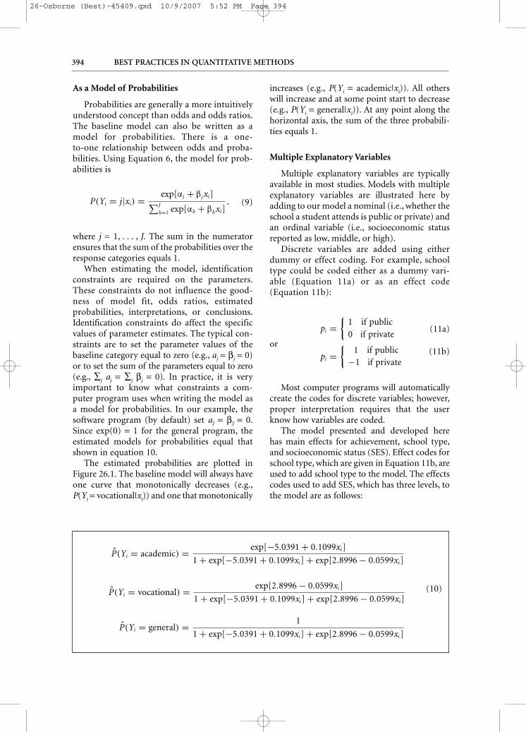
When estimating the model, identificationconstraints are required on the parameters.These constraints do not influence the good-ness of model fit, odds ratios, estimated probabilities, interpretations, or conclusions.Identification constraints do affect the specificvalues of parameter estimates. The typical con-straints are to set the parameter values of thebaseline category equal to zero (e.g., aj = βj = 0)or to set the sum of the parameters equal to zero(e.g., ∑j aj = ∑j βj = 0). In practice, it is veryimportant to know what constraints a com-puter program uses when writing the model asa model for probabilities. In our example, thesoftware program (by default) set aJ = βJ = 0.Since exp(0) = 1 for the general program, theestimated models for probabilities equal thatshown in equation 10.

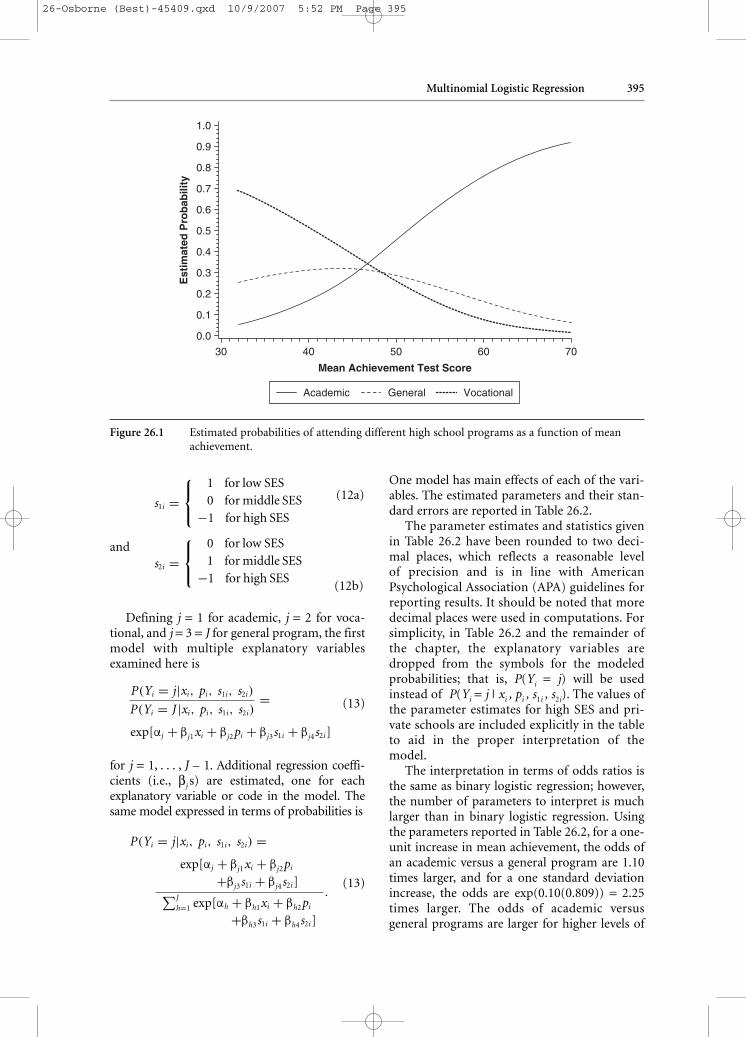
The estimated probabilities are plotted inFigure 26.1. The baseline model will always haveone curve that monotonically decreases (e.g.,P(Yi = vocational|xi)) and one that monotonically

increases (e.g., P(Yi = academic|xi)). All otherswill increase and at some point start to decrease(e.g., P(Yi = general|xi)). At any point along thehorizontal axis, the sum of the three probabili-ties equals 1.

Multiple Explanatory Variables

Multiple explanatory variables are typicallyavailable in most studies. Models with multipleexplanatory variables are illustrated here byadding to our model a nominal (i.e., whether theschool a student attends is public or private) andan ordinal variable (i.e., socioeconomic statusreported as low, middle, or high).

Discrete variables are added using eitherdummy or effect coding. For example, schooltype could be coded either as a dummy vari-able (Equation 11a) or as an effect code(Equation 11b):

or

(11a)

(11b)

Most computer programs will automaticallycreate the codes for discrete variables; however,proper interpretation requires that the userknow how variables are coded.

The model presented and developed here has main effects for achievement, school type,and socioeconomic status (SES). Effect codes forschool type, which are given in Equation 11b, areused to add school type to the model. The effectscodes used to add SES, which has three levels, tothe model are as follows:

pi ={

1 if public0 if private

pi ={

1 if public−1 if private

P(Yi = j|xi) = exp[αj + βj xi]∑J

h=1 exp[αh + βhxi],

P̂(Yi = vocational) = exp[2.8996 − 0.0599xi]

1 + exp[−5.0391 + 0.1099xi] + exp[2.8996 − 0.0599xi](10)

P̂(Yi = academic) = exp[−5.0391 + 0.1099xi]

1 + exp[−5.0391 + 0.1099xi] + exp[2.8996 − 0.0599xi]

P̂(Yi = general) = 1

1 + exp[−5.0391 + 0.1099xi] + exp[2.8996 − 0.0599xi]



30

1.0

0.9

0.8

0.7

0.6

0.5

0.4

0.3

0.2

0.1

0.0

40 50

Mean Achievement Test Score

Est

imat

ed P

rob

abili

ty

60 70

Academic General Vocational

Figure 26.1 Estimated probabilities of attending different high school programs as a function of meanachievement.

Defining j = 1 for academic, j = 2 for voca-tional, and j = 3 = J for general program, the firstmodel with multiple explanatory variablesexamined here is

(13)

for j = 1, . . . , J – 1. Additional regression coeffi-cients (i.e., βj s) are estimated, one for eachexplanatory variable or code in the model. Thesame model expressed in terms of probabilities is

(13)

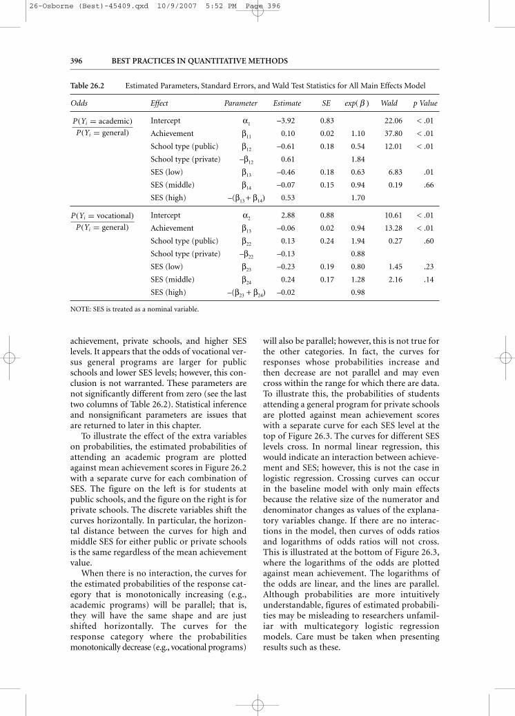
One model has main effects of each of the vari-ables. The estimated parameters and their stan-dard errors are reported in Table 26.2.

The parameter estimates and statistics givenin Table 26.2 have been rounded to two deci-mal places, which reflects a reasonable levelof precision and is in line with AmericanPsychological Association (APA) guidelines forreporting results. It should be noted that moredecimal places were used in computations. Forsimplicity, in Table 26.2 and the remainder ofthe chapter, the explanatory variables aredropped from the symbols for the modeledprobabilities; that is, P(Yi = j) will be usedinstead of P(Yi = j | xi , pi , s1i , s2i). The values ofthe parameter estimates for high SES and pri-vate schools are included explicitly in the tableto aid in the proper interpretation of themodel.

The interpretation in terms of odds ratios isthe same as binary logistic regression; however,the number of parameters to interpret is muchlarger than in binary logistic regression. Usingthe parameters reported in Table 26.2, for a one-unit increase in mean achievement, the odds ofan academic versus a general program are 1.10times larger, and for a one standard deviationincrease, the odds are exp(0.10(0.809)) = 2.25times larger. The odds of academic versus general programs are larger for higher levels of

P(Yi = j|xi, pi, s1i, s2i) =exp[αj + βj1xi + βj2pi

+βj3s1i + βj4s2i]∑J

h=1 exp[αh + βh1xi + βh2pi

+βh3s1i + βh4s2i]

.

P(Yi = j|xi, pi, s1i, s2i)

P(Yi = J |xi, pi, s1i, s2i)=

exp[αj + βj1xi + βj2pi + βj3s1i + βj4s2i]

s1i =⎧⎨⎩

1 for low SES0 for middle SES

−1 for high SES

s2i =⎧⎨⎩

0 for low SES1 for middle SES

−1 for high SES

(12a)

and

(12b)



achievement, private schools, and higher SESlevels. It appears that the odds of vocational ver-sus general programs are larger for publicschools and lower SES levels; however, this con-clusion is not warranted. These parameters arenot significantly different from zero (see the lasttwo columns of Table 26.2). Statistical inferenceand nonsignificant parameters are issues thatare returned to later in this chapter.

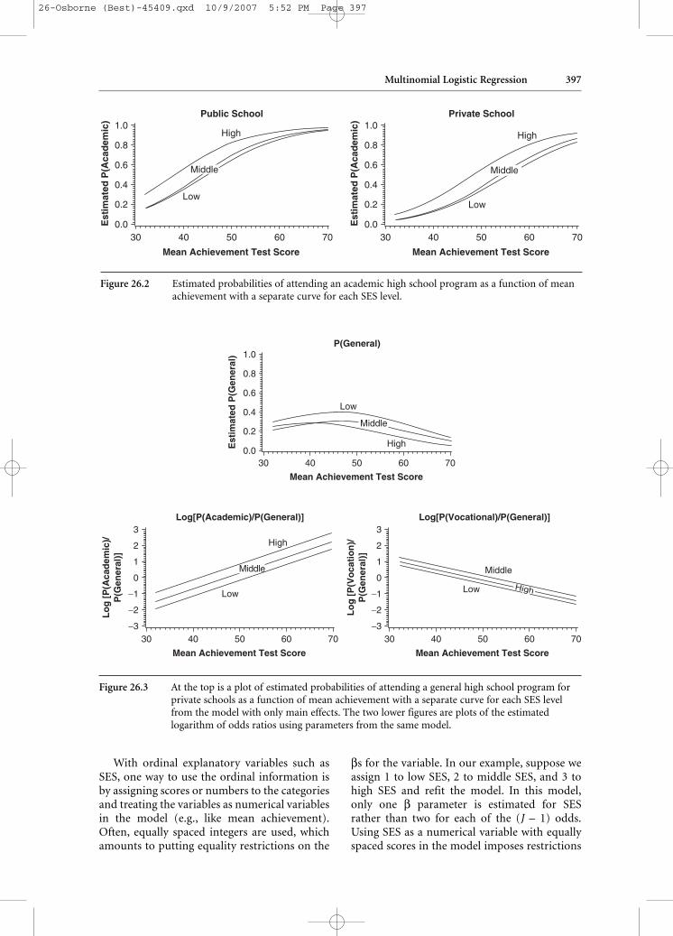
To illustrate the effect of the extra variableson probabilities, the estimated probabilities ofattending an academic program are plottedagainst mean achievement scores in Figure 26.2with a separate curve for each combination ofSES. The figure on the left is for students atpublic schools, and the figure on the right is forprivate schools. The discrete variables shift thecurves horizontally. In particular, the horizon-tal distance between the curves for high andmiddle SES for either public or private schoolsis the same regardless of the mean achievementvalue.

When there is no interaction, the curves forthe estimated probabilities of the response cat-egory that is monotonically increasing (e.g.,academic programs) will be parallel; that is,they will have the same shape and are justshifted horizontally. The curves for theresponse category where the probabilitiesmonotonically decrease (e.g., vocational programs)

will also be parallel; however, this is not true forthe other categories. In fact, the curves forresponses whose probabilities increase andthen decrease are not parallel and may evencross within the range for which there are data.To illustrate this, the probabilities of studentsattending a general program for private schoolsare plotted against mean achievement scoreswith a separate curve for each SES level at thetop of Figure 26.3. The curves for different SESlevels cross. In normal linear regression, thiswould indicate an interaction between achieve-ment and SES; however, this is not the case inlogistic regression. Crossing curves can occurin the baseline model with only main effectsbecause the relative size of the numerator anddenominator changes as values of the explana-tory variables change. If there are no interac-tions in the model, then curves of odds ratiosand logarithms of odds ratios will not cross.This is illustrated at the bottom of Figure 26.3,where the logarithms of the odds are plottedagainst mean achievement. The logarithms ofthe odds are linear, and the lines are parallel.Although probabilities are more intuitivelyunderstandable, figures of estimated probabili-ties may be misleading to researchers unfamil-iar with multicategory logistic regressionmodels. Care must be taken when presentingresults such as these.

Table 26.2 Estimated Parameters, Standard Errors, and Wald Test Statistics for All Main Effects Model

Odds Effect Parameter Estimate SE exp( β ) Wald p Value

Intercept α1 –3.92 0.83 22.06 < .01

Achievement β11 0.10 0.02 1.10 37.80 < .01

School type (public) β12 –0.61 0.18 0.54 12.01 < .01

School type (private) –β12 0.61 1.84

SES (low) β13 –0.46 0.18 0.63 6.83 .01

SES (middle) β14 –0.07 0.15 0.94 0.19 .66

SES (high) –(β13 + β14) 0.53 1.70

Intercept α2 2.88 0.88 10.61 < .01

Achievement β13 –0.06 0.02 0.94 13.28 < .01

School type (public) β22 0.13 0.24 1.94 0.27 .60

School type (private) –β22 –0.13 0.88

SES (low) β23 –0.23 0.19 0.80 1.45 .23

SES (middle) β24 0.24 0.17 1.28 2.16 .14

SES (high) –(β23 + β24) –0.02 0.98

NOTE: SES is treated as a nominal variable.

P(Yi = vocational)

P(Yi = general)

P(Yi = academic)

P(Yi = general)



With ordinal explanatory variables such asSES, one way to use the ordinal information isby assigning scores or numbers to the categoriesand treating the variables as numerical variablesin the model (e.g., like mean achievement).Often, equally spaced integers are used, whichamounts to putting equality restrictions on the

βs for the variable. In our example, suppose weassign 1 to low SES, 2 to middle SES, and 3 tohigh SES and refit the model. In this model,only one β parameter is estimated for SESrather than two for each of the (J – 1) odds.Using SES as a numerical variable with equallyspaced scores in the model imposes restrictions

30

1.0

Low

High

Middle

0.8

0.6

0.4

0.2

0.0


P(General)

Est

imat

ed P

(Gen

eral

)

40 50 60 70

Low

High

30

3

2

1

0

−2

−1

−3


Log[P(Academic)/P(General)]

Lo

g [

P(A

cad

emic

)/P

(Gen

eral

)]

40 50 60 70

Middle

Lo

g [

P(V

oca

tio

n)/

P(G

ener

al)]

30

3

2

1

0

−2

−1

−3


Log[P(Vocational)/P(General)]

40 50

Low

Middle

60 70

High

Figure 26.3 At the top is a plot of estimated probabilities of attending a general high school program forprivate schools as a function of mean achievement with a separate curve for each SES levelfrom the model with only main effects. The two lower figures are plots of the estimatedlogarithm of odds ratios using parameters from the same model.

30

1.0

0.8

0.6

0.4

0.2

0.0


Public SchoolE

stim

ated

P(A

cad

emic

)

40

Low

High High

Middle

Low

50 60 70

Middle

30

1.0

0.8

0.6

0.4

0.2

0.0


Private School

Est

imat

ed P

(Aca

dem

ic)

40 50 60 70

Figure 26.2 Estimated probabilities of attending an academic high school program as a function of meanachievement with a separate curve for each SES level.



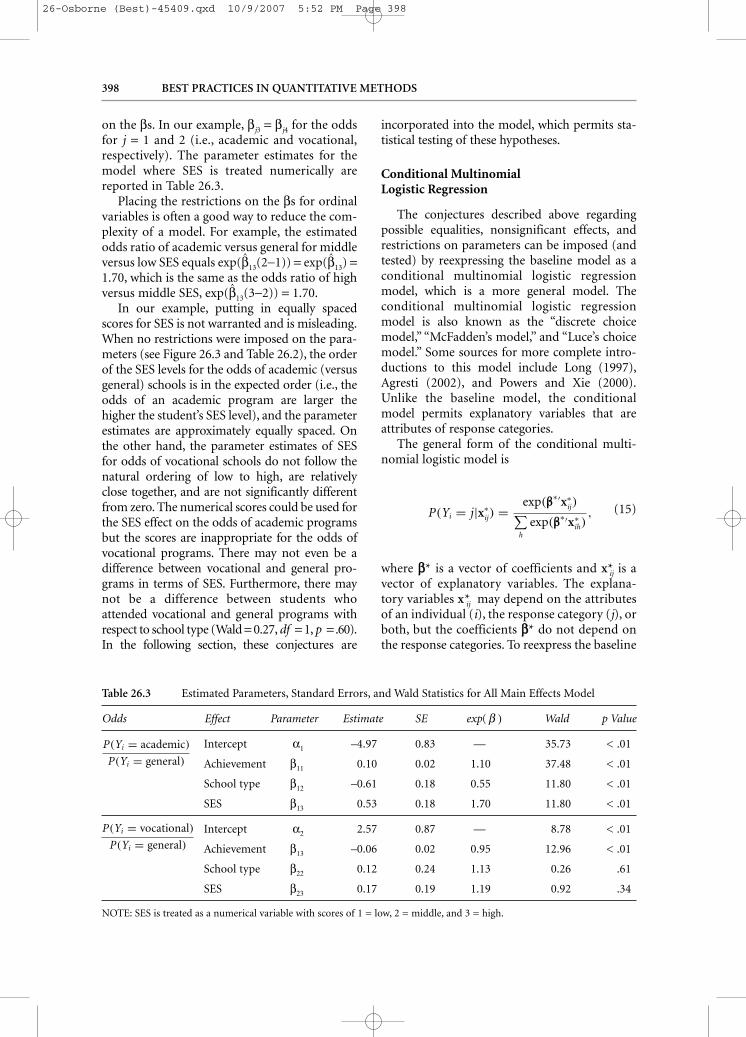
on the βs. In our example, βj3 = βj4 for the oddsfor j = 1 and 2 (i.e., academic and vocational,respectively). The parameter estimates for themodel where SES is treated numerically arereported in Table 26.3.

Placing the restrictions on the βs for ordinalvariables is often a good way to reduce the com-plexity of a model. For example, the estimatedodds ratio of academic versus general for middleversus low SES equals exp(β̂13(2−1)) = exp(β̂13) =1.70, which is the same as the odds ratio of highversus middle SES, exp(β̂13(3−2)) = 1.70.

In our example, putting in equally spacedscores for SES is not warranted and is misleading.When no restrictions were imposed on the para-meters (see Figure 26.3 and Table 26.2), the orderof the SES levels for the odds of academic (versusgeneral) schools is in the expected order (i.e., theodds of an academic program are larger thehigher the student’s SES level), and the parameterestimates are approximately equally spaced. Onthe other hand, the parameter estimates of SESfor odds of vocational schools do not follow thenatural ordering of low to high, are relativelyclose together, and are not significantly differentfrom zero. The numerical scores could be used forthe SES effect on the odds of academic programsbut the scores are inappropriate for the odds ofvocational programs. There may not even be adifference between vocational and general pro-grams in terms of SES. Furthermore, there maynot be a difference between students whoattended vocational and general programs withrespect to school type (Wald = 0.27, df = 1, p = .60).In the following section, these conjectures are

incorporated into the model, which permits sta-tistical testing of these hypotheses.

Conditional Multinomial Logistic Regression

The conjectures described above regardingpossible equalities, nonsignificant effects, andrestrictions on parameters can be imposed (andtested) by reexpressing the baseline model as aconditional multinomial logistic regressionmodel, which is a more general model. Theconditional multinomial logistic regressionmodel is also known as the “discrete choicemodel,” “McFadden’s model,” and “Luce’s choicemodel.” Some sources for more complete intro-ductions to this model include Long (1997),Agresti (2002), and Powers and Xie (2000).Unlike the baseline model, the conditionalmodel permits explanatory variables that areattributes of response categories.

The general form of the conditional multi-nomial logistic model is

(15)

where ββ* is a vector of coefficients and x*ij is avector of explanatory variables. The explana-tory variables x*ij may depend on the attributesof an individual (i), the response category (j), orboth, but the coefficients ββ* do not depend onthe response categories. To reexpress the baseline

P(Yi = j|x∗ij) = exp(β

∗′x∗ij)∑

h

exp(β∗′x∗

ih),

Table 26.3 Estimated Parameters, Standard Errors, and Wald Statistics for All Main Effects Model


Intercept α1 –4.97 0.83 — 35.73 < .01

Achievement β11 0.10 0.02 1.10 37.48 < .01

School type β12 –0.61 0.18 0.55 11.80 < .01

SES β13 0.53 0.18 1.70 11.80 < .01

Intercept α2 2.57 0.87 — 8.78 < .01

Achievement β13 –0.06 0.02 0.95 12.96 < .01

School type β22 0.12 0.24 1.13 0.26 .61

SES β23 0.17 0.19 1.19 0.92 .34

NOTE: SES is treated as a numerical variable with scores of 1 = low, 2 = middle, and 3 = high.

P(Yi = academic)

P(Yi = general)

P(Yi = vocational)

P(Yi = general)



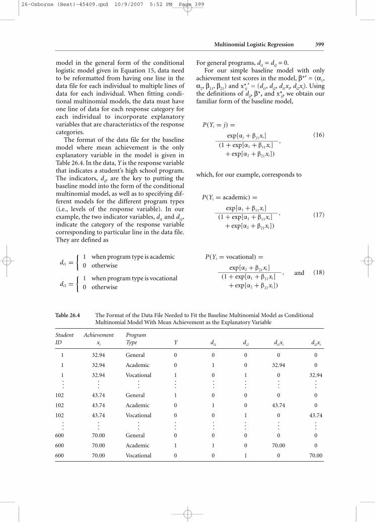
model in the general form of the conditionallogistic model given in Equation 15, data needto be reformatted from having one line in thedata file for each individual to multiple lines ofdata for each individual. When fitting condi-tional multinomial models, the data must haveone line of data for each response category foreach individual to incorporate explanatoryvariables that are characteristics of the responsecategories.

The format of the data file for the baselinemodel where mean achievement is the onlyexplanatory variable in the model is given inTable 26.4. In the data, Y is the response variablethat indicates a student’s high school program.The indicators, dij, are the key to putting thebaseline model into the form of the conditionalmultinomial model, as well as to specifying dif-ferent models for the different program types(i.e., levels of the response variable). In ourexample, the two indicator variables, di1 and di2,indicate the category of the response variablecorresponding to particular line in the data file.They are defined as

For general programs, di1 = di2 = 0.For our simple baseline model with only

achievement test scores in the model, β*′ = (α1,α2, β11, β21) and x*ij ′ = (di1, di2, di1xi, di2xi). Usingthe definitions of dij, β*, and x*ij, we obtain ourfamiliar form of the baseline model,

(16)

which, for our example, corresponds to

(17)

(18)

P(Yi = vocational) =exp[α2 + β21xi]

(1 + exp[α1 + β11xi]+ exp[α2 + β21xi])

,

P(Yi = academic) =exp[α1 + β11xi]

(1 + exp[α1 + β11xi]+ exp[α2 + β21xi])

,

P(Yi = j) =exp[αj + βj1xi]

(1 + exp[α1 + β11xi]+ exp[α2 + β21xi])

,

di1 ={

1 when program type is academic0 otherwise

di2 ={

1 when program type is vocational0 otherwise

Table 26.4 The Format of the Data File Needed to Fit the Baseline Multinomial Model as ConditionalMultinomial Model With Mean Achievement as the Explanatory Variable

Student Achievement ProgramID xi Type Y di1 di2 di1xi di2xi

1 32.94 General 0 0 0 0 0

1 32.94 Academic 0 1 0 32.94 0

1 32.94 Vocational 1 0 1 0 32.94

102 43.74 General 1 0 0 0 0

102 43.74 Academic 0 1 0 43.74 0

102 43.74 Vocational 0 0 1 0 43.74

600 70.00 General 0 0 0 0 0

600 70.00 Academic 1 1 0 70.00 0

600 70.00 Vocational 0 0 1 0 70.00

...

...

...

...

...

...

...

...

...

...

...

...

...

...

...

...

and



(19)

Note that the parameters for the last category,which in this case is general programs, were setequal to zero for identification (i.e., α31 = 0 for theintercept, and β31 = 0 for achievement test scores).

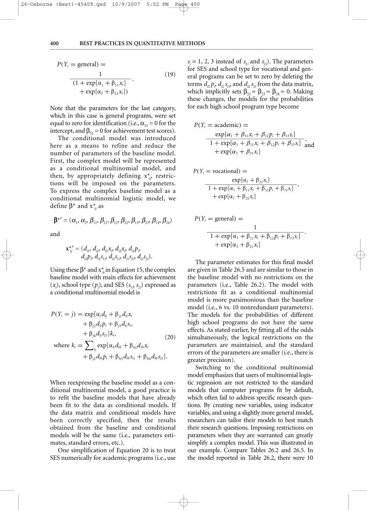
The conditional model was introducedhere as a means to refine and reduce thenumber of parameters of the baseline model.First, the complex model will be representedas a conditional multinomial model, andthen, by appropriately defining x*ij, restric-tions will be imposed on the parameters.To express the complex baseline model as aconditional multinomial logistic model, wedefine β* and x*ij as

ββ*′ = (α1, α2, β11, β21, β12, β22, β13, β23, β14, β24)

and

x*ij′ = (di1, di2, di1xi, di2xi, di1pi,di2pi, di1s1i, di2s1i, di1s2i, di2s2i).

Using these β* and x*ij in Equation 15, the complexbaseline model with main effects for achievement(xi), school type (pi), and SES (s1i, s2i) expressed asa conditional multinomial model is

When reexpressing the baseline model as a con-ditional multinomial model, a good practice isto refit the baseline models that have alreadybeen fit to the data as conditional models. Ifthe data matrix and conditional models havebeen correctly specified, then the resultsobtained from the baseline and conditionalmodels will be the same (i.e., parameters esti-mates, standard errors, etc.).

One simplification of Equation 20 is to treatSES numerically for academic programs (i.e., use

si = 1, 2, 3 instead of s1i and s2i). The parametersfor SES and school type for vocational and gen-eral programs can be set to zero by deleting theterms di2 pi, di2 s1i, and di2 s2i from the data matrix,which implicitly sets β22 = β23 = β24 = 0. Makingthese changes, the models for the probabilitiesfor each high school program type become

The parameter estimates for this final modelare given in Table 26.5 and are similar to those inthe baseline model with no restrictions on theparameters (i.e., Table 26.2). The model withrestrictions fit as a conditional multinomialmodel is more parsimonious than the baselinemodel (i.e., 6 vs. 10 nonredundant parameters).The models for the probabilities of differenthigh school programs do not have the sameeffects. As stated earlier, by fitting all of the oddssimultaneously, the logical restrictions on theparameters are maintained, and the standarderrors of the parameters are smaller (i.e., there isgreater precision).

Switching to the conditional multinomialmodel emphasizes that users of multinomial logis-tic regression are not restricted to the standardmodels that computer programs fit by default,which often fail to address specific research ques-tions. By creating new variables, using indicatorvariables, and using a slightly more general model,researchers can tailor their models to best matchtheir research questions. Imposing restrictions onparameters when they are warranted can greatlysimplify a complex model. This was illustrated inour example. Compare Tables 26.2 and 26.5. In the model reported in Table 26.2, there were 10

P(Yi = general) =1

1 + exp[α1 + β11xi + β12pi + β13si]+ exp[α2 + β21xi]

.

P(Yi = vocational) =exp[α2 + β21xi]


,

P(Yi = academic) =exp[α1 + β11xi + β12pi + β13si]


,

P(Yi = general) =1

(1 + exp[α1 + β11xi]+ exp[α2 + β21xi])

.

P(Yi = j) = exp[αj dij + βj1dij xi

+ βj2dij pi + βj3dij s1i

+ βj4dij s2i]ki,

where ki =∑

hexp[αhdih + βh1dihxi

+ βj2dihpi + βh3dihs1i + βh4dihs2i].

(20)

and


nonredundant parameters, some of which are notsignificant and others that are. An additional rea-son for going the extra step of using the condi-tional model is that novice users often succumb tothe temptation of interpreting nonsignificantparameters such as those in Table 26.2. The betterapproach is to avoid the temptation. Alternatively,researchers may simply not report the nonsignifi-cant effects even though they were in the model.This also is a poor (and misleading) practice. Table26.5 contains only 6 nonredundant parameters, all of which are significant. What is statisticallyimportant stands out, and the interpretation ismuch simpler. In our example, it is readily appar-ent that students in general and vocational pro-grams only differ with respect to achievement testscores, whereas students in academic programsand those in one of the other programs differ with respect to achievement test scores, SES, andschool type.

STATISTICAL INFERENCE

Simple statistical tests were used informally inthe previous section to examine the significanceof effects in the models discussed. The topic ofstatistical inference is explicitly taken up indetail in this section. There are two basic typesof statistical inference that are of interest: theeffect of explanatory variables and whetherresponse categories are indistinguishable withrespect to the explanatory variables.

Tests of Effects

If β = 0, then an effect is unrelated to theresponse variable, given all the other effects inthe model. The two test statistics discussed here

for assessing whether β = 0 are the Wald statisticand the likelihood ratio statistic.

Maximum likelihood estimates of the modelparameters are asymptotically normal withmean equal to the value of the parameter in thepopulation—that is, the sampling distributionof β̂ ∼ N (β, σ2

β). This fact can be used to test thehypothesis β = 0 and to form confidence inter-vals for β and odds ratios.

If the null hypothesis H0 : β = 0 is true, thenthe statistic

where SE is the estimate of σ2β, has an approxi-

mate standard normal distribution. This statisticcan be used for directional or nondirectionaltests. Often, the statistic is squared, X2 = z2, andis known as a Wald statistic, which has a sam-pling distribution that is approximately chi-square with 1 degree of freedom.

When reporting results in papers, many jour-nals require confidence intervals for effects.Although many statistical software packagesautomatically provide confidence intervals, weshow where these intervals come from, whichpoints to the relationship between the confi-dence intervals and the Wald tests. A (1 − α)%Wald confidence interval for β is

β̂ ± z(1 − α)/2(SE),

where z(1 − α)/2 is the (1 − α)/2th percentile of thestandard normal distribution. A (1 − α)% confi-dence interval for the odds ratio is found by expo-nentiating the end points of the interval for β.

As an example, consider the parameter esti-mates given in Table 26.5 of our final model from

z = β̂

SE,


Table 26.5 Estimated Parameters From the Conditional Multinomial Logistic Regression Model


Intercept β11 –4.87 0.82 35.31 < .01

Achievement β12 0.10 0.02 1.10 39.81 < .01

School type (public) β13 –0.66 0.15 0.52 20.61 < .01

School type (private) –β13 0.66 1.93

SES (low) β14 0.46 0.14 1.58 10.22 < .01

Intercept β21 2.83 0.81 12.33 < .01

Achievement β22 –0.06 0.02 0.94 1.42 < .01

P(Yi = academic)

P(Yi = general)

P(Yi = vocational)

P(Yi = general)



the previous section. The Wald statistics and cor-responding p values are reported in the seventhand eighth columns. For example, the Wald statis-tic for achievement for academic programs equals

The 95% confidence interval of β for achieve-ment equals

0.0987 ± 1.96(0.0155)→(0.06742, 0.12818),

and the 95% confidence interval for the oddsratio equals

(exp(0.06742), exp(0.12818))→(1.07, 1.14).

The ratio of a parameter estimate to its stan-dard errors provides a test for single parameters;however, Wald statistics can be used for testingwhether any and multiple linear combinations ofthe βs equal zero (Agresti, 2002; Long, 1997). SuchWald statistics can be used to test simultaneouslywhether an explanatory variable or variables havean effect on any of the models for the odds. Ratherthan present the general formula for Wald tests(Agresti, 2002; Long, 1997), the likelihood ratiostatistic provides a more powerful alternative totest more complex hypotheses.

The likelihood ratio test statistic compares themaximum of the likelihood functions of two mod-els, a complex and a simpler one. The simplermodel must be a special case of the complex modelwhere restrictions have been placed on the para-meters of the more complex model. Let ln(L(M0))and ln(L(M1)) equal the natural logarithms of themaximum of the likelihood functions for the simple and the complex models, respectively.The likelihood ratio test statistic equals

G 2 = –2(ln(L(M0)) − ln(L(M1))).

Computer programs typically provide either thevalue of the maximum of the likelihood func-tion, the logarithm of the maximum, or –2 timesthe logarithm of the maximum. If the nullhypothesis is true, then G 2 has an approximatechi-square distribution with degrees of freedomequal to the difference in the number of param-eters between the two models.

The most common type of restriction onparameters is setting them equal to zero. For

example, in the baseline model with all maineffects (nominal SES), we could set all of theparameters for SES and school type equal tozero; that is, βj2 = βj3 = βj4 = 0 for j = 1 and 2. Thecomplex model is

and the simpler model is

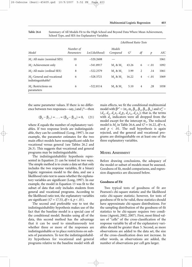
The maximum of the likelihoods of all the models estimated for this chapter arereported in Table 26.6. The difference betweenthe likelihood for these two models equals

G 2 = –2(–541.8917 + 520.26080) = 43.26.

The degrees of freedom for this test equal 6,because 6 parameters have been set equal tozero. Comparing 43.26 to the chi-square distri-bution with 6 degrees of freedom, the hypothe-sis that SES and/or school type have significanteffects is supported.

Equality restrictions on parameters can alsobe tested using the likelihood ratio test. Suchtests include determining whether an ordinalexplanatory variable can be treated numerically.For example, when SES was treated as a nominalvariable in the baseline model, SES was repre-sented in the model by βj3s1i + βj4s2i, where s1i ands2i were effect codes. When SES was treated as anumeric variable (i.e., si = 1, 2, 3 for low, middle,high), implicitly the restriction that βj3 = βj4 wasimposed, and SES was represented in the modelby βj3si. The likelihood ratio test statistic equals3.99, with df = 2 and p = .14 (see Table 26.6).Even though SES should not be treated numeri-cally for vocational and general programs, thetest indicates otherwise. It is best to treat cate-gorical explanatory variables nominally, exam-ine the results, and, if warranted, test whetherthey can be used as numerical variables.

Tests Over Regressions

A second type of test that is of interest inmultinomial logistic regression modeling iswhether two or more of the response categoriesare indistinguishable in the sense that they have

P(Yi = j)

P(Yi = J )= exp[αj + βj1xi].

P(Yi = j)

P(Yi = J )= exp[αj + βj1xi + βj2pi + βj3s1i + βj4s2i],

X 2 =(

0.0978

0.0155

)2

= 39.81.


the same parameter values. If there is no differ-ence between two responses—say, j and j*—then

(βj1 − βj*1) = . . . = (βjK − βj*K) = 0, (21)

where K equals the number of explanatory vari-ables. If two response levels are indistinguish-able, they can be combined (Long, 1997). In ourexample, the parameter estimates for the twomain effect models have nonsignificant odds forvocational versus general (see Tables 26.2 and26.3). This suggests that vocational and generalprograms may be indistinguishable.

The indistinguishability hypothesis repre-sented in Equation 21 can be tested in two ways.The simple method is to create a data set that onlyincludes the two response variables, fit a binarylogistic regression model to the data, and use alikelihood ratio test to assess whether the explana-tory variables are significant (Long, 1997). In ourexample, the model in Equation 13 was fit to thesubset of data that only includes students fromgeneral and vocational programs. According tothe likelihood ratio test, the explanatory variablesare significant (G2 = 17.53, df = 4, p < .01).

The second and preferable way to test theindistinguishability hypothesis makes use of thefact that the baseline model is a special case ofthe conditional model. Besides using all of thedata, this second method has the advantage that it can be used to simultaneously testwhether three or more of the responses areindistinguishable or to place restrictions on sub-sets of parameters. To test the indistinguishabil-ity hypotheses for vocational and generalprograms relative to the baseline model with all

main effects, we fit the conditional multinomialmodel with β*′ = (α1, α2, β11, β12, β13, β14) and x*ij′ =(di1, di2, di1xi, di1pi, di1s1i, di1s2i); that is, the termswith di2 indicators were all dropped from themodel except for the intercept α2. The reducedmodel is M4 in Table 26.6, and G2 = 16.22, df = 4,and p < .01. The null hypothesis is againrejected, and the general and vocational pro-grams are distinguishable on at least one of thethree explanatory variables.

MODEL ASSESSMENT

Before drawing conclusions, the adequacy ofthe model or subset of models must be assessed.Goodness of fit, model comparisons, and regres-sion diagnostics are discussed below.

Goodness of Fit

Two typical tests of goodness of fit arePearson’s chi-square statistic and the likelihoodratio chi-square statistic; however, for tests ofgoodness of fit to be valid, these statistics shouldhave approximate chi-square distributions. Forthe sampling distribution of the goodness-of-fitstatistics to be chi-square requires two condi-tions (Agresti, 2002, 2007). First, most fitted val-ues of “cells” of the cross-classification of theresponse variable by all of the explanatory vari-ables should be greater than 5. Second, as moreobservations are added to the data set, the size of the cross-classification does not increase. Inother words, as observations are added, thenumber of observations per cell gets larger.


Table 26.6 Summary of All Models Fit to the High School and Beyond Data Where Mean Achievement,School Type, and SES Are Explanatory Variables

Likelihood Ratio Tests

Number of Models Model Parameters Ln(Likelihood) Compared G2 df p AIC

M1: All main (nominal SES) 10 –520.2608 — 1061

M2: Achievement only 4 –541.8917 M2 & M1 43.26 6 < .01 1092

M3: All main (ordinal SES) 8 –522.2579 M3 & M1 3.99 2 .14 1061

M4: General and vocational 6 –528.3721 M4 & M1 16.22 4 < .01 1069indistinguishable?

M5: Restrictions on 6 –522.8114 M5 & M1 5.10 4 .28 1058parameters



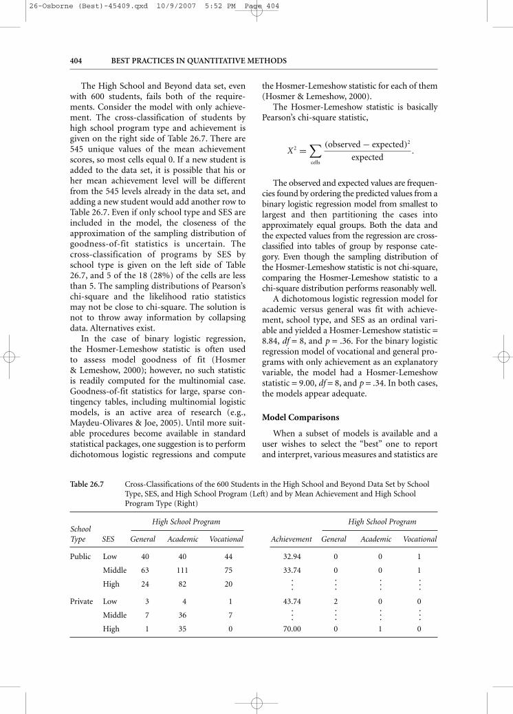
The High School and Beyond data set, evenwith 600 students, fails both of the require-ments. Consider the model with only achieve-ment. The cross-classification of students byhigh school program type and achievement isgiven on the right side of Table 26.7. There are545 unique values of the mean achievementscores, so most cells equal 0. If a new student isadded to the data set, it is possible that his orher mean achievement level will be differentfrom the 545 levels already in the data set, andadding a new student would add another row toTable 26.7. Even if only school type and SES areincluded in the model, the closeness of theapproximation of the sampling distribution ofgoodness-of-fit statistics is uncertain. Thecross-classification of programs by SES byschool type is given on the left side of Table26.7, and 5 of the 18 (28%) of the cells are lessthan 5. The sampling distributions of Pearson’schi-square and the likelihood ratio statisticsmay not be close to chi-square. The solution isnot to throw away information by collapsingdata. Alternatives exist.

In the case of binary logistic regression,the Hosmer-Lemeshow statistic is often used to assess model goodness of fit (Hosmer & Lemeshow, 2000); however, no such statistic is readily computed for the multinomial case.Goodness-of-fit statistics for large, sparse con-tingency tables, including multinomial logisticmodels, is an active area of research (e.g.,Maydeu-Olivares & Joe, 2005). Until more suit-able procedures become available in standardstatistical packages, one suggestion is to performdichotomous logistic regressions and compute

the Hosmer-Lemeshow statistic for each of them(Hosmer & Lemeshow, 2000).

The Hosmer-Lemeshow statistic is basicallyPearson’s chi-square statistic,

The observed and expected values are frequen-cies found by ordering the predicted values from abinary logistic regression model from smallest tolargest and then partitioning the cases intoapproximately equal groups. Both the data andthe expected values from the regression are cross-classified into tables of group by response cate-gory. Even though the sampling distribution ofthe Hosmer-Lemeshow statistic is not chi-square,comparing the Hosmer-Lemeshow statistic to achi-square distribution performs reasonably well.

A dichotomous logistic regression model foracademic versus general was fit with achieve-ment, school type, and SES as an ordinal vari-able and yielded a Hosmer-Lemeshow statistic =8.84, df = 8, and p = .36. For the binary logisticregression model of vocational and general pro-grams with only achievement as an explanatoryvariable, the model had a Hosmer-Lemeshowstatistic = 9.00, df = 8, and p = .34. In both cases,the models appear adequate.

Model Comparisons

When a subset of models is available and auser wishes to select the “best” one to report and interpret, various measures and statistics are

X 2 =∑cells

(observed − expected)2

expected.

Table 26.7 Cross-Classifications of the 600 Students in the High School and Beyond Data Set by SchoolType, SES, and High School Program (Left) and by Mean Achievement and High SchoolProgram Type (Right)

SchoolHigh School Program High School Program

Type SES General Academic Vocational Achievement General Academic Vocational

Public Low 40 40 44 32.94 0 0 1

Middle 63 111 75 33.74 0 0 1

High 24 82 20

Private Low 3 4 1 43.74 2 0 0

Middle 7 36 7

High 1 35 0 70.00 0 1 0

...

...

...

...

...

...

...

...


available for model comparisons. If the modelsare nested, then the conditional likelihood ratiotests discussed in the “Statistical Inference” sec-tion are possible. Although the goodness-of-fitstatistics may not have good approximations bychi-square distributions, the conditional likeli-hood ratio tests often are well approximated bychi-square distributions. One strategy is to startwith an overly complex model that gives an ade-quate representation of the data. Various effectscould be considered for removal by performingconditional likelihood ratio tests following theprocedure described earlier for testing effects inthe model.

When the subset of models is not nested,information criteria can help to choose the“best” model in the set. Information criteriaweight goodness of model fit and complexity.A common choice is Akaike’s information crite-rion (AIC), which equals

–2(maximum log likelihood – number of parameters)

(Agresti, 2002). The model with the smallestvalue of AIC is the best. The AIC values for allthe models fit in this chapter are reported inTable 26.6. The best model among those fit tothe High School and Beyond data is model M5,which is the conditional multinomial modelwith different explanatory variables for theprogram types.

When AIC statistics are very close (e.g., M1

and M3), then the choice between models mustbe based on other considerations such as inter-pretation, parsimony, and expectations. Anadditional consideration is whether statisticallysignificant effects are significant in a practicalsense (Agresti, 2007). Although many statisticscan be reported, which make model selectionappear to be an objective decision, model selec-tion is in the end a subjective decision.

Regression Diagnostics

Before any model is reported, regression diag-nostics should be performed. Lesaffre and Albert(1989) extended diagnostic procedures fordichotomous responses to the multicategory caseof multinomial logistic regression. Unfortunately,these have not been implemented in standardstatistical packages. One recommendation is to dichotomize the categories of the response,

fit binary logistic regression models, and use the regression diagnostics that are available for binary logistic regression (Hosmer &Lemeshow, 2000).

Observations may have too much influenceon the parameter estimates and the goodness offit of the model to data. Influential observationstend to be those that are extreme in terms oftheir values on the explanatory variables. Mostdiagnostics for logistic regression are general-izations of those for normal linear regression(Pregibon, 1981; see also Agresti, 2002, 2007;Hosmer & Lemeshow, 2000), but there are someexceptions (Fahrmeir & Tutz, 2001; Fay, 2002).One exception is “range-of-influence” statistics.Rather than focusing on whether observationsare outliers in the design or exert great influenceon results, range-of-influence statistics aredesigned to check for possible misclassificationsof a binary response (Fay, 2002). They are par-ticularly useful if the correctness of classifica-tions into the response categories is either verycostly or impossible to check.

PROBLEMS WITH MULTINOMIAL

REGRESSION MODELS

Two common problems encountered in multi-nomial regression models when there are multi-ple explanatory variables are multicollinearityand “quasi” or “complete separation.” As in nor-mal multiple linear regression, multicollinearityoccurs when explanatory variables are highlycorrelated. In such cases, the results can changedrastically when an explanatory variable that is correlated with other explanatory variables isadded to the model. Effects that were statisticallysignificant may no longer be significant.

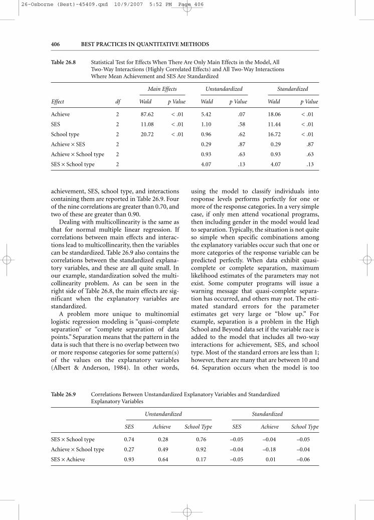
To illustrate multicollinearity, two-way inter-actions between all three main effects in ourmodel were added (i.e., between mean achieve-ment, SES as a numerical variable [1, 2, and 3],and school type). Table 26.8 contains the Waldchi-square test statistics for testing whether the βs for each effect equal zero, the degrees of free-dom, and p value for each test. The third andfourth columns contain the results for the modelwith only main effects and show that the threeeffects are statistically significant. When all two-way interactions are added to the model, nothingis significant (i.e., the fifth and sixth columns).To reveal the culprit, correlations between




Table 26.9 Correlations Between Unstandardized Explanatory Variables and Standardized Explanatory Variables

Unstandardized Standardized

SES Achieve School Type SES Achieve School Type

SES × School type 0.74 0.28 0.76 –0.05 –0.04 –0.05

Achieve × School type 0.27 0.49 0.92 –0.04 –0.18 –0.04

SES × Achieve 0.93 0.64 0.17 –0.05 0.01 –0.06

achievement, SES, school type, and interactionscontaining them are reported in Table 26.9. Fourof the nine correlations are greater than 0.70, andtwo of these are greater than 0.90.

Dealing with multicollinearity is the same asthat for normal multiple linear regression. Ifcorrelations between main effects and interac-tions lead to multicollinearity, then the variablescan be standardized. Table 26.9 also contains thecorrelations between the standardized explana-tory variables, and these are all quite small. Inour example, standardization solved the multi-collinearity problem. As can be seen in the right side of Table 26.8, the main effects are sig-nificant when the explanatory variables arestandardized.

A problem more unique to multinomiallogistic regression modeling is “quasi-completeseparation” or “complete separation of datapoints.” Separation means that the pattern in thedata is such that there is no overlap between twoor more response categories for some pattern(s)of the values on the explanatory variables(Albert & Anderson, 1984). In other words,

using the model to classify individuals intoresponse levels performs perfectly for one ormore of the response categories. In a very simplecase, if only men attend vocational programs,then including gender in the model would leadto separation. Typically, the situation is not quiteso simple when specific combinations amongthe explanatory variables occur such that one ormore categories of the response variable can bepredicted perfectly. When data exhibit quasi-complete or complete separation, maximumlikelihood estimates of the parameters may notexist. Some computer programs will issue awarning message that quasi-complete separa-tion has occurred, and others may not. The esti-mated standard errors for the parameterestimates get very large or “blow up.” Forexample, separation is a problem in the HighSchool and Beyond data set if the variable race isadded to the model that includes all two-wayinteractions for achievement, SES, and schooltype. Most of the standard errors are less than 1;however, there are many that are between 10 and64. Separation occurs when the model is too

Table 26.8 Statistical Test for Effects When There Are Only Main Effects in the Model, All Two-Way Interactions (Highly Correlated Effects) and All Two-Way Interactions Where Mean Achievement and SES Are Standardized

Main Effects Unstandardized Standardized

Effect df Wald p Value Wald p Value Wald p Value

Achieve 2 87.62 < .01 5.42 .07 18.06 < .01

SES 2 11.08 < .01 1.10 .58 11.44 < .01

School type 2 20.72 < .01 0.96 .62 16.72 < .01

Achieve × SES 2 0.29 .87 0.29 .87

Achieve × School type 2 0.93 .63 0.93 .63

SES × School type 2 4.07 .13 4.07 .13



complex for the data. The solution is to get moredata or simplify the model.

SOFTWARE

An incomplete list of programs that can fit themodels reported in this chapter is given here.The models were fit to data for this chapterusing SAS Version 9.1 (SAS Institute, Inc.,2003). The baseline models were fit usingPROC LOGISTIC under the STAT package, andthe conditional multinomial models were fitusing PROC MDC in the econometrics pack-age, ETS. Input files for all analyses reported inthis chapter as well as how to compute regres-sion diagnostics are available from the author’sWeb site at http://faculty.ed.uiuc.edu/cja/BestPractices/index.html. Also available from thisWeb site is a SAS MACRO that will computerange-of-influence statistics. Another commer-cial package that can fit both kinds of models isSTATA (StataCorp LP, 2007; see Long, 1997). Inthe program R (R Development Core Team,2007), which is an open-source version ofSPLUS (Insightful Corp., 2007), the baselinemodel can be fit to data using the glm function,and the conditional multinomial models can befit using the coxph function in the survival pack-age. Finally, SPSS (SPSS, 2006) can fit the base-line model via the multinomial logisticregression function, and the conditional multi-nomial model can be fit using COXREG.

MODELS FOR ORDINAL RESPONSES

Ordinal response variables are often found insurvey questions with response options such asstrongly agree, agree, disagree, and strongly dis-agree (or never, sometimes, often, all the time).A number of extensions of the binary logisticregression model exist for ordinal variables,the most common being the proportional oddsmodel (also known as the cumulative logitmodel), the continuation ratios model, and the adjacent categories model. Each of these is abit different in terms of how the response cate-gories are dichotomized as well as other specifics.Descriptions of these models can be found inAgresti (2002, 2007), Fahrmeir and Tutz (2001),Hosmer and Lemeshow (2000), Long (1997),Powers and Xie (2000), and elsewhere.

MANOVA, DISCRIMINANT

ANALYSIS, AND LOGISTIC REGRESSION

Before concluding this chapter, a discussion ofthe relationship between multinomial logisticregression models, multivariate analysis of vari-ance (MANOVA), and linear discriminantanalysis is warranted. As an alternative to mul-tinomial logistic regression with multipleexplanatory variables, a researcher may chooseMANOVA to test for group differences or lineardiscriminant analysis for either classificationinto groups or description of group differences.The relationship between MANOVA and lineardiscriminant analysis is well documented (e.g.,Dillon & Goldstein, 1984; Johnson & Wichern,1998); however, these models are in fact veryclosely related to logistic regression models.

MANOVA, discriminant analysis, and multi-nomial logistic regression all are applicable tothe situation where there is a single discrete vari-able Y with J categories (e.g., high school pro-gram type) and a set of K random continuousvariables denoted by X = (X1, X2, . . . , XK)′ (e.g.,achievement test scores on different subjects).Before performing discriminant analysis, it isthe recommended practice to first perform aMANOVA to test whether differences over the J categories or groups exist (i.e., H0 : µµ1 = µµ2 = . . . = µµJ, where µµj is a vector of means on theK variables). The assumptions for MANOVA arethat vectors of random variables from eachgroup follow a multivariate normal distributionwith mean equal to µµj for group j, the covariancematrices for the groups are all equal, and obser-vations over groups are independent (i.e.,Xj ~ NK (µj, ∑∑) and independent).

If the assumptions for MANOVA are met,then a multinomial logistic regression modelmust necessarily fit the data. This result is basedon statistical graphical models for discrete andcontinuous variables (Laurizten, 1996; Laurizten& Wermuth, 1989). Logistic regression is just the“flip side of the same coin.” If the assumptionsfor MANOVA are not met, then the statisticaltests performed in MANOVA and/or discrimi-nant analysis are not valid; however, statisticaltests in logistic regression will likely still be valid.In the example in this chapter, SES and schooltype are discrete and clearly are not normal. Thisposes no problem for logistic regression.

A slight advantage of discriminant analysis andMANOVA over multinomial logistic regression



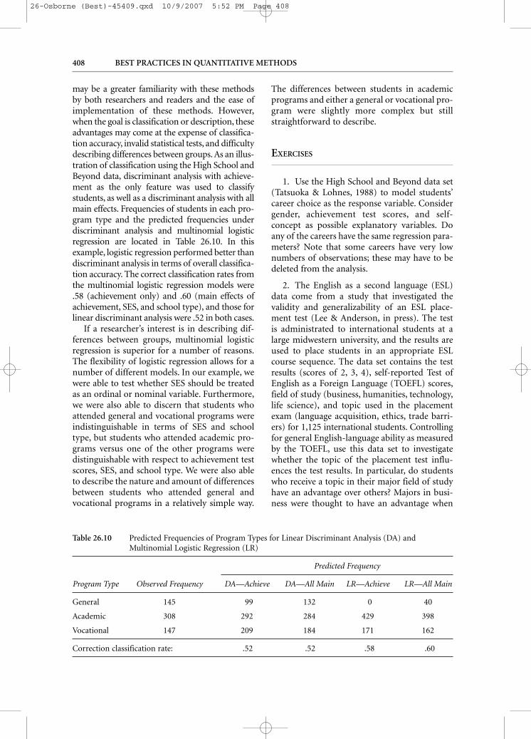
may be a greater familiarity with these methods by both researchers and readers and the ease ofimplementation of these methods. However,when the goal is classification or description, theseadvantages may come at the expense of classifica-tion accuracy, invalid statistical tests, and difficultydescribing differences between groups. As an illus-tration of classification using the High School andBeyond data, discriminant analysis with achieve-ment as the only feature was used to classifystudents, as well as a discriminant analysis with allmain effects. Frequencies of students in each pro-gram type and the predicted frequencies underdiscriminant analysis and multinomial logisticregression are located in Table 26.10. In thisexample, logistic regression performed better thandiscriminant analysis in terms of overall classifica-tion accuracy. The correct classification rates fromthe multinomial logistic regression models were.58 (achievement only) and .60 (main effects ofachievement, SES, and school type), and those forlinear discriminant analysis were .52 in both cases.

If a researcher’s interest is in describing dif-ferences between groups, multinomial logisticregression is superior for a number of reasons.The flexibility of logistic regression allows for anumber of different models. In our example, wewere able to test whether SES should be treatedas an ordinal or nominal variable. Furthermore,we were also able to discern that students whoattended general and vocational programs wereindistinguishable in terms of SES and schooltype, but students who attended academic pro-grams versus one of the other programs weredistinguishable with respect to achievement testscores, SES, and school type. We were also ableto describe the nature and amount of differencesbetween students who attended general andvocational programs in a relatively simple way.

The differences between students in academicprograms and either a general or vocational pro-gram were slightly more complex but stillstraightforward to describe.

EXERCISES

1. Use the High School and Beyond data set(Tatsuoka & Lohnes, 1988) to model students’career choice as the response variable. Considergender, achievement test scores, and self-concept as possible explanatory variables. Doany of the careers have the same regression para-meters? Note that some careers have very lownumbers of observations; these may have to bedeleted from the analysis.

2. The English as a second language (ESL)data come from a study that investigated thevalidity and generalizability of an ESL place-ment test (Lee & Anderson, in press). The test is administrated to international students at alarge midwestern university, and the results areused to place students in an appropriate ESLcourse sequence. The data set contains the testresults (scores of 2, 3, 4), self-reported Test ofEnglish as a Foreign Language (TOEFL) scores,field of study (business, humanities, technology,life science), and topic used in the placementexam (language acquisition, ethics, trade barri-ers) for 1,125 international students. Controllingfor general English-language ability as measuredby the TOEFL, use this data set to investigatewhether the topic of the placement test influ-ences the test results. In particular, do studentswho receive a topic in their major field of studyhave an advantage over others? Majors in busi-ness were thought to have an advantage when

Table 26.10 Predicted Frequencies of Program Types for Linear Discriminant Analysis (DA) andMultinomial Logistic Regression (LR)

Predicted Frequency

Program Type Observed Frequency DA—Achieve DA—All Main LR—Achieve LR—All Main

General 145 99 132 0 40

Academic 308 292 284 429 398

Vocational 147 209 184 171 162

Correction classification rate: .52 .52 .58 .60


the topic was trade, and those in humanitiesmight have had an advantage when the topicwas language acquisition or ethics. Create a vari-able that tests this specific hypothesis.

NOTE

1. See Chapter 21 (this volume) for details onPoisson regression.

REFERENCES

Agresti, A. (2002). Categorical data analysis (2nded.). New York: John Wiley.

Agresti, A. (2007). An introduction to categorical dataanalysis (2nd ed.). New York: John Wiley.

Albert, A., & Anderson, J. A. (1984). On the existenceof maximum likelihood estimates in logisticregression models. Biometrika, 71, 1–10.

Dillon, W. R., & Goldstein, M. (1984). Multivariateanalysis: Methods and applications. New York:John Wiley.

Fahrmeir, L., & Tutz, G. (2001). Multivariatestatistical modeling based on generalized linearmodels. New York: Springer.

Fay, M. P. (2002). Measuring a binary response’srange of influence in logistic regression.The American Statistician, 56, 5–9.

Hosmer, D. W., & Lemeshow, S. (2000). Applied logisticregression (2nd ed.). New York: John Wiley.

Insightful Corp. (2007). S-Plus, Version 8 [Computersoftware]. Seattle, WA: Author. Available fromhttp://www.insightful.com

Johnson, R. A., & Wichern, D. W. (1998). Appliedmultivariate statistical analysis (4th ed.).Englewood Cliffs, NJ: Prentice Hall.

Lauritzen, S. L. (1996). Graphical models. New York:Oxford University Press.

Lauritzen, S. L., & Wermuth, N. (1989). Graphicalmodels for associations between variables,some of which are qualitative and some ofwhich are quantitative. Annals of Statistics,17, 31–57.

Lee, H. K., & Anderson, C. J. (in press). Validity andtopic generality of a writing performance test.Language Testing.

Lesaffe, E., & Albert, A. (1989). Multiple-grouplogistic regression diagnostics. Applied Statistics,38, 425–440.

Long, J. S. (1997). Regression models for categoricaland limited dependent variables. ThousandOaks, CA: Sage.

Maydeu-Olivares, A., & Joe, J. (2005). Limited andfull-information estimation and goodness-of-fittesting in 2n contingency tables: A unifiedframework. Journal of the American StatisticalAssociation, 100, 1009–1020.

Powers, D. A., & Xie, Y. (2000). Statistical methods forcategorical data analysis. San Diego: AcademicPress.

Pregibon, D. (1981). Logistic regression diagnostics.Annals of Statistics, 9, 705–724.

R Development Core Team. (2007). R: A languageand environment for statistical computing[Computer software]. Vienna, Austria: Author.Available from http://www.R-project.org

SAS Institute, Inc. (2003). SAS/STAT software,Version 9.1 [Computer software]. Cary, NC:Author. Available from http://www.sas.com

SPSS. (2006). SPSS for Windows, Release 15[Computer software]. Chicago: Author.Available from http://www.spss.com

StataCorp LP. (2007). Stata Version 10 [Computersoftware]. College Station, TX: Author.Available from http://www.stata.com/products

Tatsuoka, M. M., & Lohnes, P. R. (1988). Multivariateanalysis: Techniques for educational andpsychological research (2nd ed.). New York:Macmillan.



MULTINOMIAL LOGISTIC REGRESSION - College of ...

Documents