Multilevel modeling of ozone pollution in Mexico City

Multilevel modeling of ozone pollution in Mexico

City

Oscar Borrego, Mario M. Ojeda, Patricia TapiaDepartment of Mathematics, Universidad Veracruzana

Abstract

Tropospheric ozone is one of the most damaging atmospheric pollu-tants for human health. In Mexico City this pollutant systematicallyexceeds the health official norm. In this city there is a network of at-mospheric monitoring stations, which is responsible for watching the airquality. The network reports pollutants concentration with hourly fre-quency. For knowing the potential risk population is exposed to, thestations records are not enough, but considering pollution in other loca-tions, e.g., in a regular grid, is also necessary, this is why it should beestimated.

We propose and compare ozone pollution multilevel models, consid-ering the relative humidity, the temperature, the wind speed, the winddirection and time as covariates. The covariates with significant randomeffects are identified and different continuous variance/covariance struc-tures for residuals, inspired in geostatistics, are tested. Fitting such mod-els allows plotting maps for the mean ozone and the effects of wind ineach station, which can be extended to a grid using a spatial kriging tech-nique. The data is made up of records with hourly frequency from 16monitoring stations during year 2012. The best combination of covari-ance structure and random effects is identified by means of 54 predictiontests for each station, in each test the ozone concentration is predicted bythe model fitted with data of the previous 18 hours, the errors with re-spect to the real concentration are collected and summarized as the RootMean Square Error (RMSE). The results suggest that it is more parsi-monious and suitable complicating the covariance structure than addingnew random effects. Finally we consider a model with only a randomintercept and a spherical covariance structure as the most suitable one,with a RMSE of 10.74 ppm.

Keywords: Linear Mixed Effects,

1 Introduction

In Mexico City, atmospheric pollution is the main environmental issue.According to the report about air quality in Mexico City for 2011, pub-lished by the Environment Department [16], air quality in Mexico Cityexhibits an improvement for almost all of the regarded pollutants, what

1

is attributed to the application of different environmental prevention pro-grams during the last twenty years. Nevertheless, ozone and particulatematter PM10 and PM2.5 (smaller than 10 and 2.5 µm in diameter re-spectively) are the exception. For ozone, an increase of 2.5 ppb in theyear average was reported, while the year averages for PM10 and PM2.5increased in 5 µg/m3 and 3 µg/m3, respectively.

Vehicular transit remains as the most important source of pollution inthe city. During the day, the greatest concentration of primary pollutantswere reported between 6:00 and 12:00 hours, while for ozone, due to thephoto-chemical reactions of hydrocarbons and nitrogen oxids, the greatestconcentration were reported between 12:00 and 18:00 hours [16].

With regard to the observance of the Official Mexican Standards forenvironmental health, in 2011, 449 hours with ozone concentration greaterthan 110 ppb (which is the official standard for one hour) were recorded,while the value of the fifth maximum for the 8 hours average was 120ppb [16].

During the last two decades, several public health studies have con-firmed the statistically significant associations between outdoor concen-trations of tropospheric ozone and a wide range of adverse outcomes [14],including premature mortality, hospital admissions for respiratory disease,urgent care visits, asthma attacks and restrictions in activity.

In this city there is a network of atmospheric monitoring stations(SIMAT, the Spanish acronym for Sistema de Monitoreo Atmosferico),which is responsible for watching the air quality in the region. This net-work reports pollutants concentration with hourly frequency. For knowingthe potential risk population is exposed to, the stations records are notenough, but considering pollution in other locations, e.g., in a regular grid,is also necessary, this is why it should be estimated.

In [3] a spatial analysis of ozone pollution is carried out, confirmingthe relationship among ozone and some meteorological variables, but thespatial prediction models used do not express in a suitable way the mul-tivariate nature of this phenomenon. Another important limitation isthe non-consideration of time, restricting the study to the purely spatialaspects.

In this work we propose ozone pollution multilevel models, consideringthe relative humidity, the temperature, the wind speed, the wind directionand time as covariates. The covariates with significant random effectsare identified and different continuous variance/covariance structures forresiduals, inspired in geostatistics, are tested.

Several physical-chemical numerical methods and others based on stochas-tic models have been applied for studying ozone concentration, but to thebest of our knowledge, the multilevel approach has not been applied inthis context.

1.1 Multilevel models

In social sciences, when phenomena are studied from a quantitative ap-proach, it is frequent to find or generate data aggregated in more thanone level. The classical example comes from educational statistics, whenthere is data associated to students in different schools. In this case, if

2

a linear model is proposed for a regression analysis, generally it is notsuitable assuming that the stochastic components are independently andidentically distributed (i.i.d.). Since students are nested in schools, thecovariance structure may be different for students in the same school andstudents in different schools. These issues led to finding models that in-tegrate individual and group information, the linear mixed effects modelsovercome those limitations from the linear regression analysis approach.

In school effectiveness research, researchers realized that consideringgroup structure could yield dependencies between individual observations.The emphasis was on regression analysis and on data of two levels, let’s saystudents and schools. Repeating the analysis for each school separatelywas not enough, because frequently samples within schools were small andregression coefficients were unstable. Furthermore, in large scale studiesthere were thousands of schools and long lists of regression coefficients didnot provide enough data reduction to be useful. [7]

In the mid-1980s, educational researchers realized that the models theywere looking for had been proposed already in other areas of statistics.Under different names, they were known either as mixed linear models or,in a Bayesian context, as hierarchical linear models. The realization thatthe problems of contextual analysis could be embedded in this classicallinear model framework gave rise to what we now call multilevel analysis.Thus, multilevel analysis can be defined as the marriage of contextualanalysis and traditional statistical mixed model theory. [7]

The notion of individuals, or any other type of objects, that are nat-urally nested in groups, with membership in the same group leading to apossible correlation between the individuals, turned out to be very com-pelling in many disciplines. It generalizes the notion of intraclass correla-tion to a regression context. Moreover, the notion of regressing regressioncoefficients, or using slopes-as-outcomes, is an appealing way to code in-teractions and to introduce a particular structure for the dependencieswithin groups.[7]

This kind of approaches is rarely applied in Earth sciences. The maincontribution of this study is proposing multilevel models for ozone, thatnot only help to understand the phenomenon in a geographical region,but can also be used for forecasting.

2 Mixed Linear Model

The mixed linear model (MLM) is written as

Y = Xβ + Zu+ e (1)

where

• Y is a random vector with n components,

• X ∈ Rn×r and β ∈ Rr are, respectively, the matrix of covariates andthe vector of coefficients associated to the fixed effects,

• Z ∈ Rn×p, and u are, respectively, the matrix of covariates and thevector of p random coefficients, associated to the random effects, and

3

(e

u

)∼ N

((0

0

),

(Σ 00 Ω

)).

Thus, we have Y ∼ N (Xβ, V ) with V = ZΩZ′ + Σ. We assume thatboth X and Z have full column rank.

This fact expresses the consequences of introducing random coeffi-cients: the effects of the covariates in Z do not appear in the mean, butin the covariance structure.

2.1 Two levels model

In a two levels model, we have observations aggregated into groups, forexample, records of tests for students in different schools. We denotethe i-th observation for group j as yij , while xij ∈ Rr and zij ∈ Rqare respectively the vectors of covariates for the fixed and random effectsassociated to observation ij, eij is the level 1 error term and uj is thevector of q random coefficients for group j. Let m be the number ofgroups (level 2 units) and nj the number of observations (level 1 units)for group j, we have

∑mi=1 nj = n. Then, model (1) can be written as:

Yj = Xjβ + Zjuj + ej (2)

Where

Yj =

y1j...

ynjj

, Xj =

x′1j...

x′njj

, Zj =

z′1j...

z′njj

, ej =

e1j...

enjj

,

and (ejuj

)∼ N

((0

0

),

(Σj 00 Ωj

)).

We assume that either the residuals or the random effects from differ-ent groups are uncorrelated, thus Cov (ej1 , ej2) = 0 and Cov (uj1 , uj2) = 0for j1 6= j2. Generally it is assumed that the covariance structure for ujis invariant over individuals, this is Ωj1 = Ωj2 for any j1, j2, further-more, these matrices are often modeled as diagonal or proportional to theidentity.

Since

Y =

Y1

...Ym

,

we have that

X =

X1

...Xm

, Z =

Z1 . . . 0...

. . ....

0 . . . Zm

, u =

u1

...um

, e =

e1...em

,

4

and

Ω =

Ω1 . . . 0...

. . ....

0 . . . Ωm

, Σ =

Σ1 . . . 0...

. . ....

0 . . . Σm

.

Therefore

V =

Z1Ω1Z′1 + Σ1 . . . 0...

. . ....

0 . . . ZmΩmZ′m + Σm

.

2.2 Estimation

When the Ωj and the Σj are known the standard estimator for β is thegeneralized least squares estimator

β =(X ′V −1X

)−1X ′V −1Y, (3)

while the standard predictor for u is the posterior mean

u = ΩZ′V −1(Y −Xβ).

The likelihood expression for the parameters is given by the normaldensity expression:

L(β, θ|Y ) =1√

(2π)n|V |exp

(−1

2(Y −Xβ)′V −1(Y −Xβ)

), (4)

where θ is the vector of unique parameters in Ω and Σ. Then the log-likelihood is given by

logL(β, θ|Y ) = −n2

log(2π)− 1

2log |V | − 1

2(Y −Xβ)′V −1(Y −Xβ), (5)

removing the constant term of this expression, the maximum likelihood(ML) estimation problem is formulated as

(βML, θML) ∈ arg maxβ,θ

fML(β, θ) := −1

2log |V |− 1

2(Y −Xβ)′V −1(Y −Xβ).

Since the ML estimators do not take into account the loss in degrees offreedom from the estimation of β in the variance components model [12],they are biased downward. The restricted maximum likelihood methodcorrects this bias by defining estimates of the variance components asthe maximizers of the log-likelihood based on linearly independent errorcontrasts. This log-likehood is [12]:

fRML(θ) := −1

2log |X ′V −1X|+ fML(β, θ), (6)

where β is the generalized least squares estimator defined in equation (3).In [8], [9] or [12] the reader can find a detailed development and dis-

cussion about several estimation approaches.

5

2.3 Correlation structure for level 1 residuals

En los modelos de datos repetidos, generalmente no es aceptable la hipotesisde independencia para los residuos de nivel 1, es por ello que se propo-nen diferentes estructuras para sus matrices de varianzas-covarianzas. Enparticular, si las observaciones son relativamente cercanas en el tiempo,la hipotesis de independencia no es adecuada. Es por ello que se hacenecesario considerar modelos que explıcitamente reconocen la posibili-dad de una estructura de correlacion para los eit correspondientes a unmismo individuo (unidad de nivel 2). Para residuos de nivel 1 correspon-dientes a diferentes individuos, sı se considera la ausencia de correlacion:Cov (eit, ejr) = 0 para i 6= j.

Entre los primeros modelos que daban respuesta a esta problematicafigura el siguente modelo estacionario [9]:

Cov(eit, ei(t+s)

)= σ2

e exp(−αsc),

donde α, c > 0 y σ2e = Cov (eit, eit) = Var (eit).

Este modelo permite que la separacion entre ocasiones sea continuay ademas variable entre individuos y en el tiempo. Tambien se refleja elhecho de que la correlacion decrece, tendiendo a cero, en la medida en ques crece. En el caso particular de c = 1, este modelo es el analogo continuode un proceso autorregresivo de primer orden (AR(1)).

2.3.1 Continuous time models

Discrete time models are not very suitable if time lags are not constant(i.e. not fixed time intervals) or if there is missing data. Even if datais collected at equally spaced time points, there is often variation in theobserved intervals, and failure to recognize this may lead to inefficiencyand biased estimates of the autocorrelation parameters [9].

In order to overcome these limitations, continuous time covariancemodels can be considered. Goldstein et al. (1994) propose a generalcovariance structure for the level 1 residuals:

Cov(eit, ei(t−s)

)= σ2

ef(α, s) = σ2e exp(−g(α, s)) (7)

where g(α, s) is any positive increasing function of s, not necessarilylinear, and α is a vector of parameters.

The simplest choice for g(·, ·) could be the analogue to the AR(1)process:

g(α, s) = αs.

Another possible choice is the polynomial:

g(α, s) =

q∑k=0

αksk, (8)

constrained to be positive. Inverse polynomial terms could also be con-sidered:

g(α, s) =

q2∑k=−q1

αksk,

with q1, q2 ∈ Z+, which is still linear in the parameters and can avoid highcorrelations associated with the ordinary polynomial.

6

2.4 Geo-statistical covariance models

In geo-statistics literature, particularly in the one related to the krigingmethodology (see [1], [5], or [6]), different covariance structures have beenproposed, studied in detail and validated in practice. Here we mentionsome of those models:

Spherical model h(s) =

σ2o

(1− 3|s|

2ρ+ |s|3

2ρ3

)if |s| ≤ ρ

0 if |s| > ρ

Exponential model h(s) = σ2o exp (−3|s|/ρ)

Gaussian model h(s) = σ2o exp

(−3|s|2/ρ2

).

Where the parameter ρ, called range, controls a kind of limit for thetime lag s, such that for larger lags the covariance is zero or almost zero,while the parameter σ2

o , called sill, is the limit of the covariance whenthe time lag goes to zero. In order to tolerate certain discontinuity ofthe covariance at the origin, the function h(·) is extended as h∗(s) =h(s) + Ind(s = 0)σ2

ε , where Ind(·) is the indicator function (evaluates to 1if its argument is true and 0 otherwise) and σ2

ε , called nugget effect, refersto the discontinuity of h∗ at the origin.

For any of the previous models, we can use a covariance structure givenby

Cov(eit, ei(t−s)

)= h∗(s), (9)

in such cases, we have σ2e = σ2

o + σ2ε .

Note that the exponential and gaussian models are particular cases ofthe polynomial model (8).

2.4.1 More complex covariance structures

In some applications the autocorrelation parameter may be a function oftime, with the level 1 variance remaining constant. Group differences inσ2e can be incorporated by specifying suitable dummy variables. In contin-

uous time models the parameters αk can be functions of other explanatoryvariables [9]. Hence, a more general formula for (7) is

Cov(eit, ei(t−s)

)= σ2

ef(α, s, i, t) = σ2e exp(−g(α, s, i, t)). (10)

This model is not any more stationary, since the covariance depends ontime. For instance, an extension of the linear model for g(·, ·) is

g(α, s, i, t) = (α0 + α′1zi + α′2xit)s

where xit and zi are vectors of covariates of levels 1 and 2 respectively.

7

2.5 Models comparison

For identifying the model that explains the data the best, it is necessaryto consider certain criteria, such as maximizing the likelihood, or minimiz-ing the Bayesian Information Criterion (BIC) or the Akaike InformationCriterion (AIK) [4]. However, those criteria do not provide statistical ev-idence of a model superiority in the sense of its explanatory power. Thatis why we consider the Likelihood Ratio Test (see [13, 10]). This is astatistical test used for comparing two nested models, i.e., comparing onemodel to another one that contains a subset of the parameters includedin the first model.

The test is used as follows: Let M0 and M1 be two models, where M0

contains a subset of the parameters included in M1, and let L(M0) andL(M1) be their likelihoods respectively. Then, the statistic D is definedas:

D = −2 log(L(M0)L(M1)

)= 2 logL(M1)− 2 logL(M0).

Since M1 has greater or equal likelihood than M0, we have that D > 0.The null hypothesis H0 implies that M1 is not better than M0. Under H0,D follows a χ2 distribution with degrees of freedom equal to the differencein number of parameters between M0 and M1 (this is the number ofparameters included in M1 that are not included in M0). The rejectionof H0 means that M1 is significantly better than M0 (with the specifiedsignificance level).

3 Methodology

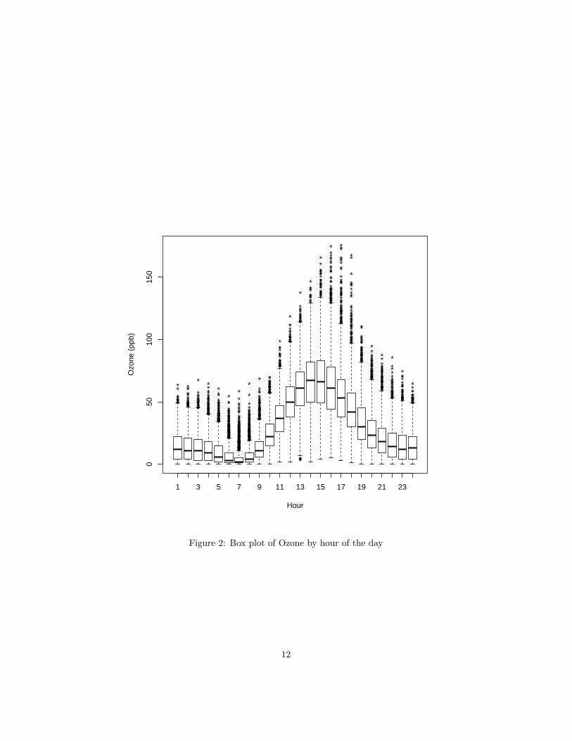
Ozone has a daily periodical pattern because of the effects of solar radia-tion during the day (see figure 2). In order to capture this pattern in themodel we consider trigonometric functions of the hour of the day. Sinceozone concentration can also be affected by the season of the year, it isalso convenient considering trigonometric functions of the moment of theyear we are referring to. These possible temporal trends may mislead theanalysis and be a cause of non-stationarity.

The proposed yearly recurrence trend model is given by sums of trigono-metric functions with frequency values given by the first two multiples ofω1:

f1(t) =

2∑k=1

ak sin(kω1T ) + bk cos(kω1T ), (11)

where T represents the time elapsed from the beginning of the year mea-sured in hours, and ω1 = 2π

365.25×24, therefore, the period is 365.25 × 24,

the number of hours in a Julian year.The proposed daily recurrence trend model is given by sums of trigono-

metric functions with frequency values given by the first two multiples ofω2:

f2(t) =

2∑k=1

a′k sin(kω2t) + b′k cos(kω2t) (12)

8

where t represents the time elapsed from the beginning of the day mea-sured in hours, and ω2 = 2π

24, therefore the period is 24 hours.

The data is made up of records with hourly frequency from 16 mon-itoring stations during year 2012. Each record of the dataset has thefollowing information:

Column Measure unit

Station identification -Date -Hour of the day hoursOzone concentration ppmTemperature degree CelsiusRelative humidity percentWind speed Km/hourWind direction Azimuth degrees

The wind information is expressed in a polar coordinate system, but forthis study it is convenient transforming such data into a Cartesian coor-dinate system. We make such transformation applying Principal Compo-nent Analysis (see [11]) from the wind data, for identifying two orthogonaldirections, one of them, the one of largest variability.

Finally, the covariates extracted from data are:

Abbreviation Variable

SINT1 sin(ω1T )SINT2 sin(2ω1T )COST1 cos(ω1T )COST2 cos(2ω1T )SINH1 sin(ω2t)SINH2 sin(2ω2t)COSH1 cos(ω2t)COSH2 cos(2ω2t)TMP TemperatureRH Relative Humidity

WSP1 1st component of windWSP2 2nd component of wind

Several multilevel models are fitted, where the second level units arethe monitoring stations, which group the records taken over time (occa-sion), and these occasions are the first level units.

The study is divided in two stages. In the first stage the significantfixed and random effects are identified.

In the second stage several combinations of covariance structures andrandom effects are compared. Due to its huge computational cost, it is notpossible to carry out this task for the whole dataset, instead only threedays are considered: April 25th to 27th, 2012. The criteria for choosingthose days were the data availability for the different stations and theseason of the year, when relatively high ozone concentrations have beenhistorically recorded. In this case the effects associated to the yearly

9

periodic behavior have been removed, since they do not make sense anymore.

In order to compare the models in stage 2, 54 time window predictiontests were performed for each station, with a window width of 18 hours.Each time window test involves predicting the ozone concentration forthe next hour by the model fitted with data of the previous 18 hours, theerrors with respect to the real concentration are collected and summarizedas the Root Mean Square Error (RMSE).

3.1 Software

In this work, all the computations have been performed and all the graph-ics have been generated using the platform R [15]. R is a free softwareproject that provides a framework for computational statistics and graph-ics generation, over a programming language of the same name. It iswidely used by researchers from diverse disciplines, due to the compu-tation facilities it offers, its availability for several operating systems, aswell as the large number of packages of specific purpose available in itsrepositories.

In particular, the multilevel models have been fitted with the pack-age multilevel [2], this package includes functions for estimating commonwithin-group agreement and reliability indices. The package also containsbasic data manipulation functions that facilitate the analysis of multileveland longitudinal data. Some of the graphics have been generated withthe packages ggplot2 [18] and scales [19].

The ordinary kriging algorithm used for drawing the map in figure 4was implemented in R by the authors.

4 Exploratory analysis

Figure 1 shows scatter graphs for ozone versus TMP, RH, WSP1 andWSP2. It is known that ozone concentration is somehow correlated withTMP and RH, positively and negatively respectively, (see for example[3]). These phenomena are confirmed by the scatter graphs. With regardto WSP1 and WSP2, there are not very clear patterns, in this sense, therandom effects may be helpful since in different stations the main effectsof wind could manifest in different directions.

Figure 2 shows a box plot for ozone concentration by hour of the day,where the expected pattern is observed. This graph suggests that theaverage pattern can be described by trigonometric functions of time withperiod of 24 hours, which justifies the idea of considering the trigonometriccovariates.

5 Results for stage 1

Seven multilevel models, denoted as M1. . .M7, have been considered. Thefollowing table describes the effects for each model, where F means fixedeffect and FR means both fixed and random:

10

0

50

100

150

0 10 20 30

TMP

Ozo

ne

0

50

100

150

0 25 50 75 100

RH

Ozo

ne

0

50

100

150

−8 −4 0 4

WSP1

Ozo

ne

0

50

100

150

−3 0 3

WSP2

Ozo

ne

Figure 1: Scatter plots for 2012 SIMAT data, Ozone vs TMP, RH, WSP1 andWSP2

11

****

*

*****

****** *

*

*****

*

*

*

***

*

*****************

***** *

****

*

****

*

*

*****

************************

*****

*

*

*

***

*

****

*

*

*

*************************

*******

*********

****

*

*

***

*

*

********

*

*****

******

**

***

**

*

***********************************

**

*

****

**

*

*******

*********

**********

*

****

**

****

*

**

*

**********

*

*

******

*

*

***

**

**

****

**

****

*

**

*

****

*

*

**

*****

*

*

***

***********

*******

****

******

*

********

*

**********

***

*****

*

*****

*

*

*

***

**

*********

*

***********

*****

*****

**

*

*

***

**

***

***

**

*

*

*

*

*

**

*********

*

****

*******

*

************

**

*********************

******

***********

*********

**

*

*

*

*

*

****

***

*

*

*

*****

**

**

*

**

***

*

**

*****

**

*

*

*

****

*

***

**

*

******

*

**

******

*

**

**

*

*

*****

*

*

***

***

*

****

*

****

*

**

*

**********

*

*******

*****

**

*

***

*

*

**

*

*****

*

**

*

***

****

*

*******

***

*********

*

******

*

*

*

******

*

*

***

*

*

*******

*

*

*

**

****

****

*****

*********************

*

***

*

***

*********

*

***

*****

********

**

**

**

**

*

*

***

**

***

*

**

***

*

*

*

****

*

*

*

****

*

**

*

**

*

***

*

**

******

*****

**

*

************

**

*

**

****

*

***

**

**

**

*

***

*

*

*

*

**

*

****

*

***

*

****

****************

*

***

********

*

*

*

*

*********

**

*

***

*

*

****

*

****

**

****

*

**

***

**

**

*

*

******

*

**

******

****

******

*

***

**

************

*

**************************

*

*

*

****

*

***

*

***

*

********

****************

*

*******

**

*

******

*

********

********************************

*

***

*

*

******

*************

*

***

*

*

*

**

***

*

**

****

**

*****

*

**********

*

**

*

***

*******

*

***

**********

*

*******

******

*

***

******

***********

**********************

***

****

*

****

**

*

****

*

****

*

****

*

******

**

**

**********

****

*

**

*

*

*

*

*

*

*

******

**

*

************

*

*

**

*

********

*

***

*

*

*

*

*

****

*

**

*

***

*

*

**

*

*

*

*

**

*

*

*

***

****

*

*

*********

*

*

*

***

*

*

*

*

*

**

*

***

*

*

*

*

*

*

*

*

*

*

*

**

*

*

*

*

*

*

*

*

*

*

*

*

*

****

*

*

*

*

*

***

*

*

*

****

*

**

*

***

*

**

*

***

*

*

*****

*

*

****

*

*

*

*

*

*

*

***

*

*

***

*

*

****

*

***

**

*

*

*

*

*

*

*

**

*

*

*

*

*

***

*

***

*

**

**

*

*

**

**

*

*

***

*

*****

*

*

*********

*****

*

***

*

*

*

***

****

**

*

*

******

*

*

*

*********

*

*

*

**

*

****

********

***

*

*

***

*

**

*****

*****

*

**

*

********

*

*****

****

*

**

****

*******

**

*

*******

*

***

*

*****

*

**

*

**********

*

*

***

*

*

*

*

**************

*

*

* *

*

**

*

**********

**

**

****

******

*

*

*****

********************

*

**********

1 3 5 7 9 11 13 15 17 19 21 23

050

100

150

Hour

Ozo

ne (

ppb)

Figure 2: Box plot of Ozone by hour of the day

12

Effects M1 M2 M3 M4 M5 M6 M7

(Intercept) FR FR FR FR FR FR FRSINT1 F F F F F F FSINT2 F F F F F F FSINH1 F F F F F F FSINH2 F F F F F F FCOSH1 F F F F F F FCOSH2 F F F F F F FTMP F F F F F FRH F F F F FWSP1 F F FR FRWSP2 F F FR

For all of these models we assume residuals are i.i.d. ∼ N(0, σ2

e

),

this is a very simple and common variance/covariance structure, but thisassumption might not be very suitable (back on this below).

Including random effects for TMP and RH yielded unsuitable resultscompared with similar and simpler models, this is due to their effects overozone concentration are invariant over space, i.e. they are not significantlydifferent for different geographical locations, in contrast with the effectsof wind.

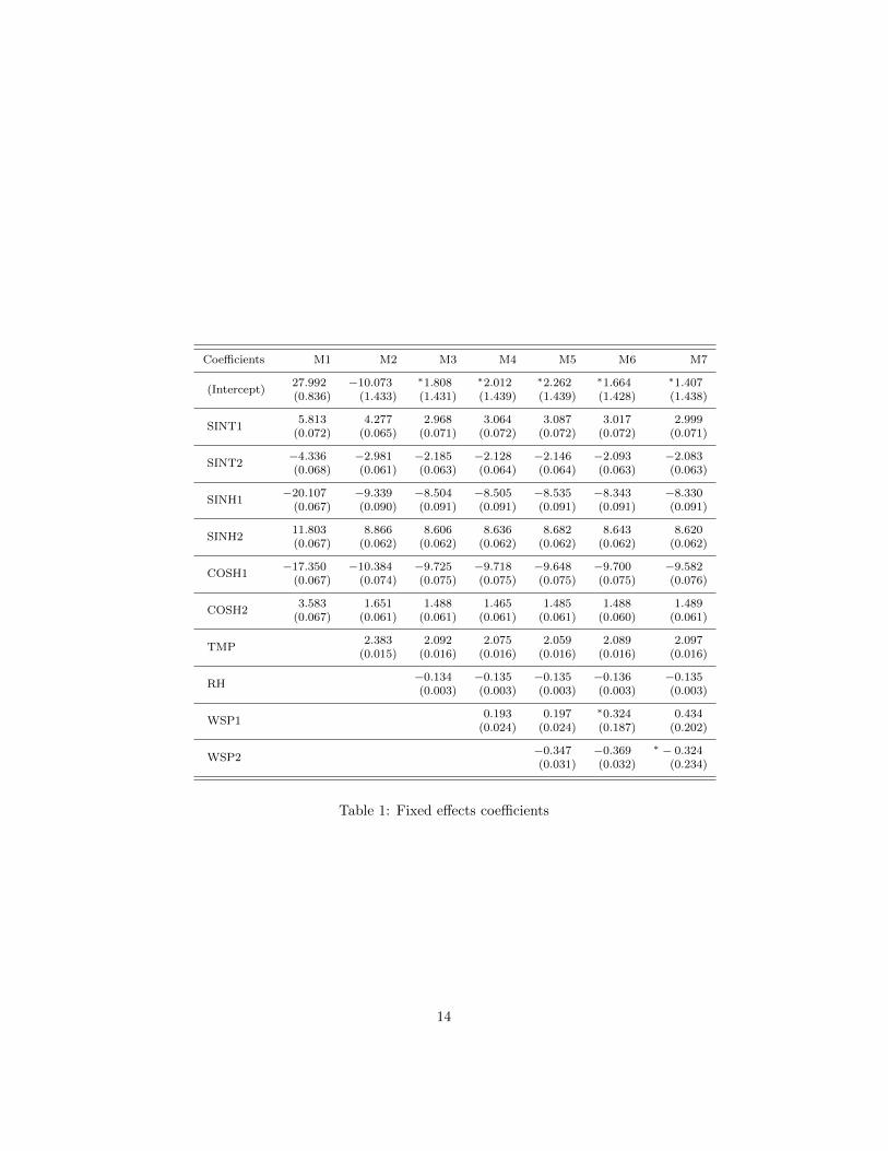
Table 1 presents the coefficients fitted for the models, the standarderrors appear in brackets. The asterisk at the left of the coefficient meansthat it is non-significant with α = 0.05.

The fixed effects of the Intercept are non-significant for most of themodels, this is due to the new covariates and the random effects explainbetter the behavior of ozone concentration, and its intercept is practically0.

The coefficients of TMP are positive, as expected, and near 2 for everymodel, this means that on average, for each degree the temperature in-creases, the ozone concentration increases in 2 ppm. Similarly, the effectsof RH are negative and near -0.135 for every model, i.e. on average, anincrease in 10% of RH involves a decrease of 1.35 ppm in ozone concen-tration.

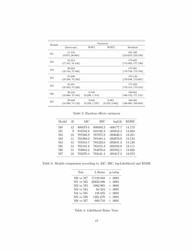
Table 2 shows the variances (and their 95% confidence intervals) forthe randoms effects and the residuals associated to each model. In can benoted that the more complex the model the smaller the variance of theresiduals.

Table 3 shows the degrees of fredom and goodness of fit measures:AIC, BIC, log-Likelihood, RMSE. Table 4 shows several Likelihood RatioTests results. Model M0 is a simple linear model with the same fixedeffects than M7. As expected, the most complex models have the bestgoodness of fit according to all the criteria, and are significantly betterwith regard to the Likelihood Ratio tests. Model M2 is more suitablethan M0, even though the first one has fewer parameters, that is to saythat considering the trigonometric covariates, temperature and a randomintercept is preferable than including all the fixed effects in a simple linearmodel.

13

Coefficients M1 M2 M3 M4 M5 M6 M7

(Intercept)27.992 −10.073 ∗1.808 ∗2.012 ∗2.262 ∗1.664 ∗1.407(0.836) (1.433) (1.431) (1.439) (1.439) (1.428) (1.438)

SINT15.813 4.277 2.968 3.064 3.087 3.017 2.999

(0.072) (0.065) (0.071) (0.072) (0.072) (0.072) (0.071)

SINT2−4.336 −2.981 −2.185 −2.128 −2.146 −2.093 −2.083(0.068) (0.061) (0.063) (0.064) (0.064) (0.063) (0.063)

SINH1−20.107 −9.339 −8.504 −8.505 −8.535 −8.343 −8.330

(0.067) (0.090) (0.091) (0.091) (0.091) (0.091) (0.091)

SINH211.803 8.866 8.606 8.636 8.682 8.643 8.620(0.067) (0.062) (0.062) (0.062) (0.062) (0.062) (0.062)

COSH1−17.350 −10.384 −9.725 −9.718 −9.648 −9.700 −9.582

(0.067) (0.074) (0.075) (0.075) (0.075) (0.075) (0.076)

COSH23.583 1.651 1.488 1.465 1.485 1.488 1.489

(0.067) (0.061) (0.061) (0.061) (0.061) (0.060) (0.061)

TMP2.383 2.092 2.075 2.059 2.089 2.097

(0.015) (0.016) (0.016) (0.016) (0.016) (0.016)

RH−0.134 −0.135 −0.135 −0.136 −0.135(0.003) (0.003) (0.003) (0.003) (0.003)

WSP10.193 0.197 ∗0.324 0.434

(0.024) (0.024) (0.187) (0.202)

WSP2−0.347 −0.369 ∗ − 0.324(0.031) (0.032) (0.234)

Table 1: Fixed effects coefficients

14

ModelsVariances

(Intercept) WSP1 WSP2 Residual

M111.132 221.565

(6.074, 26.664) (219.619, 223.536)

M231.914 175.627

(17.415, 76.445) (174.084, 177.190)

M330.683 172.261

(16.743, 73.495) (170.748, 173.794)

M431.039 172.149

(16.938, 74.350) (170.638, 173.681)

M531.031 171.924

(16.933, 74.329) (170.414, 173.454)

M630.544 0.549 169.621

(16.668, 73.165) (0.299, 1.314) (168.132, 171.131)

M730.949 0.642 0.861 168.361

(16.888, 74.133) (0.350, 1.537) (0.470, 2.062) (166.883, 169.859)

Table 2: Random effects variances

Model df AIC BIC logLik RMSE

M0 12 800379.4 800493.3 -400177.7 14.173M1 9 810102.8 810188.3 -405042.4 14.884M2 10 787280.9 787375.9 -393630.5 13.251M3 11 785380.0 785484.4 -392679.0 13.124M4 12 785318.7 785432.6 -392647.3 13.120M5 13 785191.8 785315.3 -392582.9 13.111M6 15 783934.2 784076.6 -391952.1 13.022M7 18 783270.4 783441.4 -391617.2 12.972

Table 3: Models comparison according to AIC, BIC, log-Likelihood and RMSE

Test L.Ratio p-value

M0 vs M7 17120.948 < .0001M1 vs M2 22823.886 < .0001M2 vs M3 1902.965 < .0001M3 vs M4 63.324 < .0001M4 vs M5 128.835 < .0001M5 vs M6 1261.670 < .0001M6 vs M7 669.710 < .0001

Table 4: Likelihood Ratio Tests

15

(Intercept) WSP1 WSP2

ACO 2.541 −0.200 0.624CHO 1.115 0.434 −0.029CUA 9.230 0.752 0.844FAC −2.486 0.689 1.920HGM −5.695 0.825 −1.274MER −9.735 0.106 −1.275MON 3.724 −0.398 1.308NEZ −4.096 0.013 −1.267PED 2.007 −0.436 −0.274SAG −5.626 0.131 0.872SFE 6.933 0.308 −0.383SUR −4.260 1.144 −0.682TAH 5.745 −0.535 −0.269TLA −6.641 −0.359 −0.489TPN 7.651 −2.440 −0.200VIF −0.407 −0.035 0.573

Table 5: M7 random effects

5.1 Model M7 random effects

Table 5 shows the random effects fitted for model M7 by monitoring sta-tion.

Let a and b be the total effects (fixed plus random) associated to WSP1and WSP2, it is not hard to prove (e.g. using the Lagrange multipliers

theorem) that the vector(a/√a2 + b2, b/

√a2 + b2

)Tin the coordinate

system induced by WSP1 and WSP2 is the unitary vector of maximumimpact on the ozone concentration, i.e. if wind blows in that direction itscontribution to ozone is maximum, this contribution is of

√a2 + b2 ppm

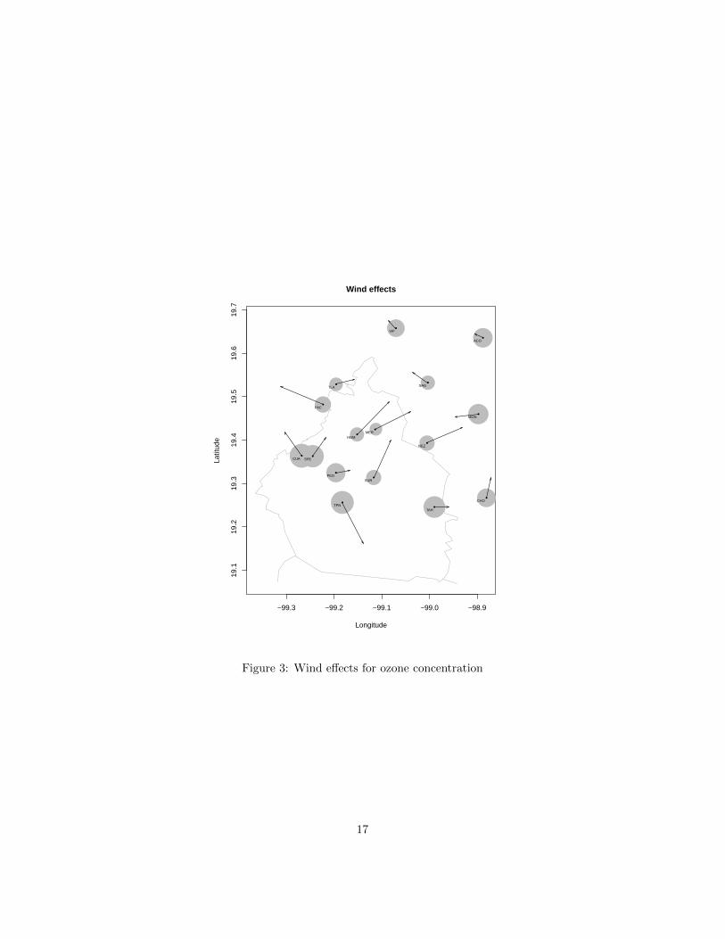
for each km/h on speed.Those wind effects are illustrated in figure 3, where the radii of circles

are proportional to the intercept effects, the arrows indicate the directionsof maximum impact and their length is proportional to that impact. Thismap shows that the southwestern region is, on average, more polluted(such fact has also been reported in [3]), this is explained by the higherconcentration of factories in the zone. And that is consistent with thewind directions of maximum impact (Northeast, East and Southeast) formany of the monitoring stations.

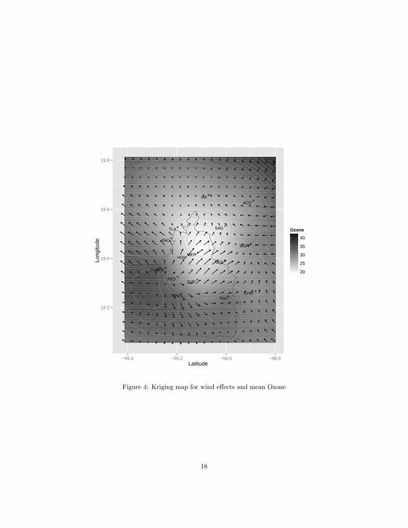
Figure 4 shows a map generated by kriging from the same informationof figure 3. A better illustration of the previous remarks can be appreci-ated, confirming that the Southwestern region is a kind of pollution focusand if wind blows in direction Northeast this can transport the ozoneclouds to the most populated regions of the valley.

16

−99.3 −99.2 −99.1 −99.0 −98.9

19.1

19.2

19.3

19.4

19.5

19.6

19.7

Wind effects

Longitude

Latit

ude

ACO

CHO

CUA

FAC

HGMMER

MON

NEZ

PED

SAG

SFE

SUR

TAH

TLA

TPN

VIF

Figure 3: Wind effects for ozone concentration

17

ACO

CHO

CUA

FAC

HGMMER

MON

NEZ

PED

SAG

SFE

SUR

TAH

TLA

TPN

VIF

19.2

19.4

19.6

19.8

−99.4 −99.2 −99.0 −98.8Latitude

Long

itude

20

25

30

35

40

Ozone

Figure 4: Kriging map for wind effects and mean Ozone

18

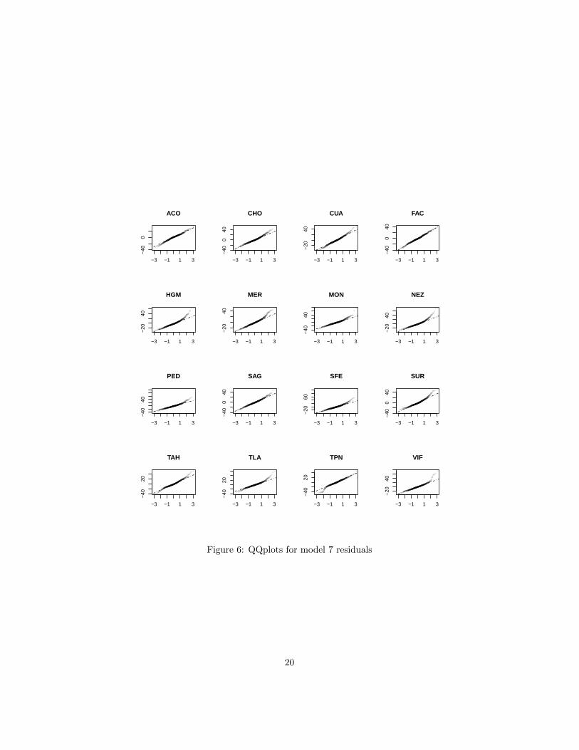
5.2 Model M7 residuals normality

In order to test the hypothesis of normality for model M7, figure 5 showsa QQplot of its residuals. The graphs suggests that such assumption doesnot hold. Similiar QQplots are presented in figure 6 by each station.Stations like ACO, FAC, SAG or MON seem to hold this hypothesis, butit is clearly not the case for HGM, NEZ, MER, TLA or VIF.

−4 −2 0 2 4

−4

−2

02

46

8

Theoretical Quantiles

Sam

ple

Qua

ntile

s

Figure 5: QQplot for model 7 residuals

19

−3 −1 1 3

−40

0

ACO

−3 −1 1 3

−40

040

CHO

−3 −1 1 3

−20

40

CUA

−3 −1 1 3

−40

040

FAC

−3 −1 1 3

−20

40

HGM

−3 −1 1 3

−20

40

MER

−3 −1 1 3

−40

40

MON

−3 −1 1 3

−20

40

NEZ

−3 −1 1 3

−40

40

PED

−3 −1 1 3

−40

040

SAG

−3 −1 1 3

−20

60

SFE

−3 −1 1 3

−40

040

SUR

−3 −1 1 3

−40

20

TAH

−3 −1 1 3

−40

20

TLA

−3 −1 1 3

−40

20

TPN

−3 −1 1 3

−20

40

VIF

Figure 6: QQplots for model 7 residuals

20

On suspicion of non-fulfillment of the model assumptions, a Bartletttest for equal variances was applied (see [17]). The residuals were groupedby hour of the day, yielding the following results: Bartlett’s K-squared =20402.15, df = 23, p-value < 0.001, thus the hypothesis of homoscedastic-ity is rejected with a significance level of 0.05. This suggests that a morecomplex covariance structure should be considered.

21

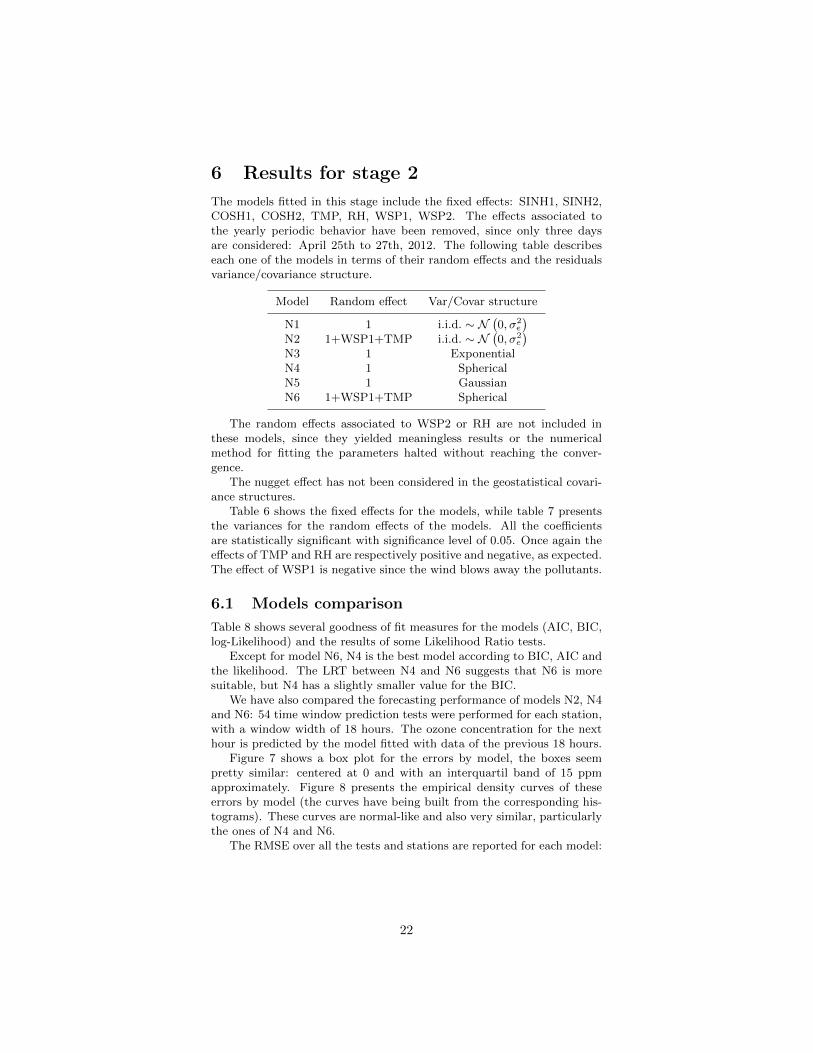
6 Results for stage 2

The models fitted in this stage include the fixed effects: SINH1, SINH2,COSH1, COSH2, TMP, RH, WSP1, WSP2. The effects associated tothe yearly periodic behavior have been removed, since only three daysare considered: April 25th to 27th, 2012. The following table describeseach one of the models in terms of their random effects and the residualsvariance/covariance structure.

Model Random effect Var/Covar structure

N1 1 i.i.d. ∼ N(0, σ2

e

)N2 1+WSP1+TMP i.i.d. ∼ N

(0, σ2

e

)N3 1 ExponentialN4 1 SphericalN5 1 GaussianN6 1+WSP1+TMP Spherical

The random effects associated to WSP2 or RH are not included inthese models, since they yielded meaningless results or the numericalmethod for fitting the parameters halted without reaching the conver-gence.

The nugget effect has not been considered in the geostatistical covari-ance structures.

Table 6 shows the fixed effects for the models, while table 7 presentsthe variances for the random effects of the models. All the coefficientsare statistically significant with significance level of 0.05. Once again theeffects of TMP and RH are respectively positive and negative, as expected.The effect of WSP1 is negative since the wind blows away the pollutants.

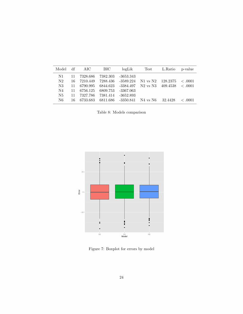
6.1 Models comparison

Table 8 shows several goodness of fit measures for the models (AIC, BIC,log-Likelihood) and the results of some Likelihood Ratio tests.

Except for model N6, N4 is the best model according to BIC, AIC andthe likelihood. The LRT between N4 and N6 suggests that N6 is moresuitable, but N4 has a slightly smaller value for the BIC.

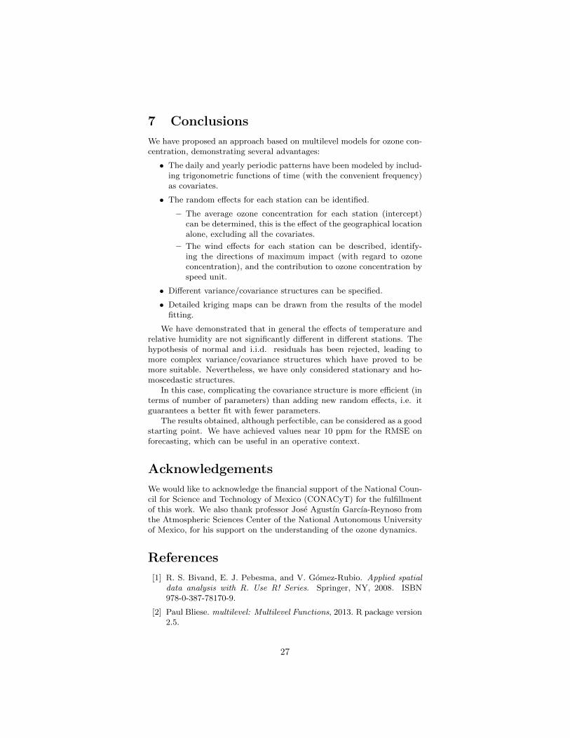
We have also compared the forecasting performance of models N2, N4and N6: 54 time window prediction tests were performed for each station,with a window width of 18 hours. The ozone concentration for the nexthour is predicted by the model fitted with data of the previous 18 hours.

Figure 7 shows a box plot for the errors by model, the boxes seempretty similar: centered at 0 and with an interquartil band of 15 ppmapproximately. Figure 8 presents the empirical density curves of theseerrors by model (the curves have being built from the corresponding his-tograms). These curves are normal-like and also very similar, particularlythe ones of N4 and N6.

The RMSE over all the tests and stations are reported for each model:

22

Coefficients N1 N2 N3 N4 N5 N6

(Intercept)44.875 38.433 39.641 38.596 44.930 35.445(4.005) (5.597) (5.913) (5.400) (3.997) (6.484)

SINH1−24.446 −18.412 −19.836 −20.980 −24.507 −18.669

(1.561) (1.586) (2.022) (1.947) (1.537) (1.945)

SINH211.185 10.798 10.225 10.441 11.163 10.260(0.492) (0.457) (0.679) (0.720) (0.481) (0.680)

COSH1−18.374 −15.223 −15.634 −16.388 −18.405 −15.347

(0.962) (0.953) (1.319) (1.243) (0.952) (1.215)

COSH22.719 2.796 2.754 2.662 2.715 2.625

(0.481) (0.444) (0.674) (0.717) (0.481) (0.674)

TMP0.507 0.867 0.675 0.671 0.503 0.829

(0.174) (0.273) (0.260) (0.239) (0.172) (0.303)

RH−0.426 −0.516 −0.463 −0.389 −0.425 −0.409(0.063) (0.062) (0.085) (0.081) (0.063) (0.080)

WSP1−3.927 −2.988 −2.148 −2.316 −3.921 −2.060(0.257) (0.465) (0.299) (0.282) (0.255) (0.427)

Table 6: Fixed effects coefficients

ModelsVariances

(Intercept) WSP1 TMP Residual

N122.523 100.636

(12.072, 56.020) (92.268, 110.203)

N2253.941 2.184 0.657 83.408

(136.115, 631.614) (1.171, 5.432) (0.352, 1.633) (76.472, 91.337)

N325.424 112.466

(13.627, 63.234) (103.114, 123.158)

N427.138 99.434

(14.546, 67.500) (91.166, 108.887)

N522.464 100.540

(12.041, 55.873) (92.179, 110.097)

N6222.293 1.479 0.511 88.977

(119.151, 552.895) (0.793, 3.678) (0.274, 1.272) (81.579, 97.436)

Table 7: Random effects variances

23

Model df AIC BIC logLik Test L.Ratio p-value

N1 11 7328.686 7382.303 -3653.343N2 16 7210.449 7288.436 -3589.224 N1 vs N2 128.2375 < .0001N3 11 6790.995 6844.623 -3384.497 N2 vs N3 409.4538 < .0001N4 11 6756.125 6809.753 -3367.063N5 11 7327.786 7381.414 -3652.893N6 16 6733.683 6811.686 -3350.841 N4 vs N6 32.4428 < .0001

Table 8: Models comparison

−20

0

20

N2 N4 N6Model

Err

or

Figure 7: Boxplot for errors by model

24

0.00

0.01

0.02

0.03

0.04

−20 0 20Error

dens

ity

Model

N2

N4

N6

Figure 8: Histograms for errors by model

25

Model RMSE

N2 10.80419N4 10.74120N6 10.18795

Model N2 yields similar (worst) results than N4, even though it hasa greater number of parameters. This demonstrates that in this caseit is preferable a more complex covariance structure for the intra-groupresiduals than adding random effects, since it is more parsimonious andsuitable for data. On the other hand, model N6 leads N4 in the RMSE byapproximately 0.6 ppm, but this relatively small improvement has beenachieved at the expense of four additional parameters.

This is why we consider model N4 is the most suitable one.Figure 9 presents a QQplot graph for the residuals of model N4. Al-

though the match between sample and theoretical quantiles is not as ex-pected according to the assumptions of the model (particularly for quan-tiles of larger absolute value), this one is better than the one of figure5.

−3 −2 −1 0 1 2 3

−3

−2

−1

01

23

Theoretical Quantiles

Sam

ple

Qua

ntile

s

Figure 9: QQplot for model N4 residuals

26

7 Conclusions

We have proposed an approach based on multilevel models for ozone con-centration, demonstrating several advantages:

• The daily and yearly periodic patterns have been modeled by includ-ing trigonometric functions of time (with the convenient frequency)as covariates.

• The random effects for each station can be identified.

– The average ozone concentration for each station (intercept)can be determined, this is the effect of the geographical locationalone, excluding all the covariates.

– The wind effects for each station can be described, identify-ing the directions of maximum impact (with regard to ozoneconcentration), and the contribution to ozone concentration byspeed unit.

• Different variance/covariance structures can be specified.

• Detailed kriging maps can be drawn from the results of the modelfitting.

We have demonstrated that in general the effects of temperature andrelative humidity are not significantly different in different stations. Thehypothesis of normal and i.i.d. residuals has been rejected, leading tomore complex variance/covariance structures which have proved to bemore suitable. Nevertheless, we have only considered stationary and ho-moscedastic structures.

In this case, complicating the covariance structure is more efficient (interms of number of parameters) than adding new random effects, i.e. itguarantees a better fit with fewer parameters.

The results obtained, although perfectible, can be considered as a goodstarting point. We have achieved values near 10 ppm for the RMSE onforecasting, which can be useful in an operative context.

Acknowledgements

We would like to acknowledge the financial support of the National Coun-cil for Science and Technology of Mexico (CONACyT) for the fulfillmentof this work. We also thank professor Jose Agustın Garcıa-Reynoso fromthe Atmospheric Sciences Center of the National Autonomous Universityof Mexico, for his support on the understanding of the ozone dynamics.

References

[1] R. S. Bivand, E. J. Pebesma, and V. Gomez-Rubio. Applied spatialdata analysis with R. Use R! Series. Springer, NY, 2008. ISBN978-0-387-78170-9.

[2] Paul Bliese. multilevel: Multilevel Functions, 2013. R package version2.5.

27

[3] O. Borrego-Hernandez, M. M. Ojeda-Ramırez, J. A. Garcıa-Reynoso,and C. R. Castro-Lopez. Interpolacion espacial de concentracionesde ozono en la zona metropolitana del valle de mexico, basadaen metodos de kriging y cokriging. In Concepcion RodrıguezPuebla, Antonio Ceballos Barbancho, Nube Gonzalez Reviriego, En-rique Moran Tejeda, and Ascension Hernandez Encinas, editors,Cambio climatico. Extremos e Impacto. Serie A, 8, pages 281–290,Salamanca, Espana, 2012. Asociacion Espanola de Climatologıa,Publicaciones de la Asociacion Espanola de Climatologıa. ISBN:978-84-695-4331-3.

[4] Kenneth P. Burnham and David R. Anderson. Multimodel inference:Uniderstanding aic and bic in model seleciton. Sociological Methods& Research, 33:261–304, 2004.

[5] Noel A. C. Cressie. Statistics for spatial data. Wiley series in prob-ability and mathematical statistics, New York, 1993. ISBN 0-471-84336-9.

[6] Noel A. C. Cressie and C. K. Wikle. Statistics for spatio-temporaldata. Wiley Series in Probability and Statistics, New Jersey, 2011.

[7] Jan de Leeuw and Erik Meijer. Introduction to multilevel analysis. InJan de Leeuw and Erik Meijer, editors, Handbook of Multilevel Anal-ysis, pages 1–75. University of California,University of Groningen,Springer, 2008.

[8] Harvey Goldstein. Multilevel Statistical Models 4th Edition. JohnWiley & Sons Inc. Series in Probability and Statistics, West Sussex,United Kingdom, 2011.

[9] Harvey Goldstein, Michael J. R. Healy, and Jon Rasbash. Multi-level time series models with applications to repeated measures data.Statistics in Medicine, 13:1643–1655, 1994.

[10] J. P. Huelsenbeck and K. A. Crandall. Phylogeny estimation and hy-pothesis testing using maximum likelihood. Annual Review of Ecologyand Systematics, 28:437–466, 1997.

[11] W. Hardle and L. Simar. Applied multivariate statistical analysis,Second Edition. Springer, Berlin Heidelberg New York, 2007.

[12] Mary J. Lindstrom and Douglas M. Bates. Newton-raphson andem-algorithms for linear mixed-effects models for repeated-measuresdata. JASA, 83(404):1014–1022, December 1998.

[13] J. Neyman and E.S. Pearson. On the problem of the most efficienttests of statistical hypotheses. Phil. Trans. R. Soc. Lond. A, 231:289–337, 1933.

[14] Bart D. Ostro, Hien Tran, and Jonathan I. Levy. The health benefitsof reduced tropospheric ozone in california. Journal of Air & WasteManage Association, 56:1007–1021, July 2006. ISSN 1047-3289.

[15] R Development Core Team. R: A Language and Environment forStatistical Computing. R Foundation for Statistical Computing, Vi-enna, Austria, 2013. ISBN 3-900051-07-0.

28

[16] SIMAT. Calidad del aire en la Ciudad de Mexico. Informe 2011.Sistema de Monitoreo Atmosferico, Secretarıa del Medio Ambiente,Distrito Federal, Mexico, 2012.

[17] G.W. Snecdecor and W.G. Cochran. Statistical Methods. Wiley, 1991.ISBN 9780813815619.

[18] Hadley Wickham. ggplot2: elegant graphics for data analysis.Springer New York, 2009.

[19] Hadley Wickham. scales: Scale functions for graphics., 2012. Rpackage version 0.2.3.

29

Multilevel modeling of ozone pollution in Mexico City

Documents