Banco de M´ exico Documentos de Investigaci´ on Banco de M´ exico Working Papers N ◦ 2007-09 Multifactor Productivity and its Determinants: An Empirical Analysis for Mexican Manufacturing H´ ector Salgado Banda Lorenzo E. Bernal Verdugo Banco de M´ exico Banco de M´ exico May 2007 La serie de Documentos de Investigaci´ on del Banco de M´ exico divulga resultados preliminares de trabajos de investigaci´ on econ´ omica realizados en el Banco de M´ exico con la finalidad de propiciar el intercambio y debate de ideas. El contenido de los Documentos de Investigaci´ on, as´ ı como las conclusiones que de ellos se derivan, son responsabilidad exclusiva de los autores y no reflejan necesariamente las del Banco de M´ exico. The Working Papers series of Banco de M´ exico disseminates preliminary results of economic research conducted at Banco de M´ exico in order to promote the exchange and debate of ideas. The views and conclusions presented in the Working Papers are exclusively the responsibility of the authors and do not necessarily reflect those of Banco de M´ exico.

Welcome message from author
This document is posted to help you gain knowledge. Please leave a comment to let me know what you think about it! Share it to your friends and learn new things together.
Transcript
Banco de Mexico
Documentos de Investigacion
Banco de Mexico
Working Papers
N◦ 2007-09
Multifactor Productivity and its Determinants:An Empirical Analysis for Mexican Manufacturing
Hector Salgado Banda Lorenzo E. Bernal VerdugoBanco de Mexico Banco de Mexico
May 2007
La serie de Documentos de Investigacion del Banco de Mexico divulga resultados preliminares detrabajos de investigacion economica realizados en el Banco de Mexico con la finalidad de propiciarel intercambio y debate de ideas. El contenido de los Documentos de Investigacion, ası como lasconclusiones que de ellos se derivan, son responsabilidad exclusiva de los autores y no reflejannecesariamente las del Banco de Mexico.
The Working Papers series of Banco de Mexico disseminates preliminary results of economicresearch conducted at Banco de Mexico in order to promote the exchange and debate of ideas. Theviews and conclusions presented in the Working Papers are exclusively the responsibility of theauthors and do not necessarily reflect those of Banco de Mexico.
Documento de Investigacion Working Paper2007-09 2007-09
Multifactor Productivity and its Determinants:An Empirical Analysis for Mexican Manufacturing*
Hector Salgado Banda† Lorenzo E. Bernal Verdugo‡
Banco de Mexico Banco de Mexico
AbstractWe use data from the Annual Industrial Survey for 1996-2003. First, we estimate produc-
tion functions by means of growth accounting exercises and panel data econometrics for thewhole sector and for 14 comprehensive groups. Various measures of Multifactor Productivity(MFP) are constructed, as we consider diverse combinations of inputs with capital, labour,electricity and transport. This allows us to compare MFP growth rates between groups. Sec-ond, we analyse econometrically some of the determinants of MFP and Labour Productivity(LP) growth. We find that, on the one hand, there is some evidence of a positive relationshipbetween market concentration and technology adoption; on the other hand, both technologyadoption and human capital seem to be promoting productivity, whilst market concentrationis exerting a negative influence on it. In sum, our results suggest that, once controlling forthe effect on technology adoption, more concentration (conversely, less competition) has anegative impact on productivity.Keywords: Panel data, Productivity, Manufacturing, Competition.JEL Classification: C33, D24, L11
ResumenSe usan datos de la Encuesta Industrial Anual de 1996 a 2003. Primero, se estiman
funciones de produccion con contabilidad de crecimiento y econometrıa de datos de panelpara el sector y para 14 grupos. Se construyen varias medidas de Productividad Multifactorial(PMF) al considerar diversas combinaciones de insumos con capital, trabajo, electricidady transporte. Esto permite comparar tasas de crecimiento de la PMF entre los distintosgrupos. Segundo, se analizan econometricamente algunos de los determinantes de la PMF yde la Productividad Laboral (PL). Se encuentra que, por una parte, existe evidencia de unarelacion positiva entre concentracion de mercado y adopcion tecnologica; por otra parte, tantoadopcion tecnologica como capital humano parecen estar promoviendo la productividad,mientras que la concentracion de mercado tiene una influencia negativa sobre ella. En suma,los resultados parecen sugerir que, una vez que se controla por el efecto sobre la adopciontecnologica, una mayor concentracion (inversamente, menor competencia) tiene un impactonegativo sobre la productividad.Palabras Clave: Panel de datos, Productividad, Manufacturas, Competencia.
*D. Flores provided outstanding research assistance. We are very grateful to D. Chiquiar for his guidancein this study. We also thank C. Capistran, A. Dıaz de Leon, A. Gaytan, E. Martınez and seminar participantsat Banco de Mexico and 2006 LACEA-LAMES for helpful comments. G. Leyva, A. Duran and O. Soto wereof great help answering our doubts about the data. Any errors are the sole responsibility of the authors.
† Direccion General de Investigacion Economica. Corresponding author.Email: [email protected].
‡ Direccion General de Investigacion Economica. Email: [email protected].
1 Introduction
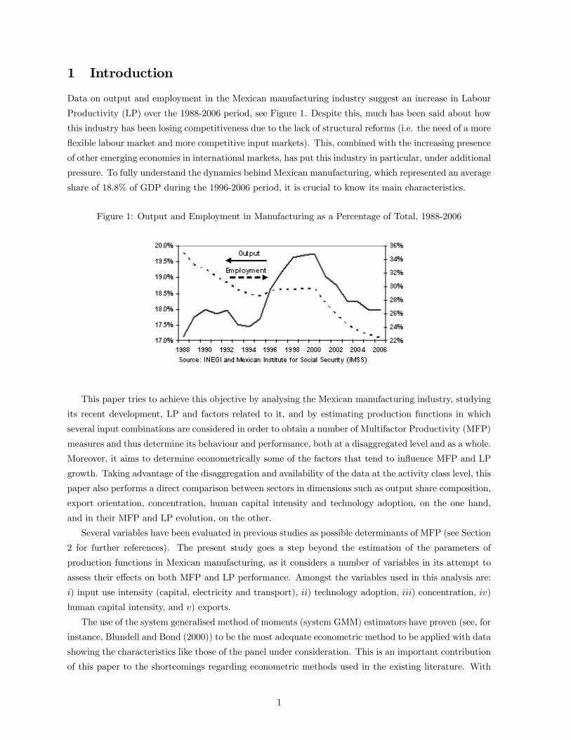
Data on output and employment in the Mexican manufacturing industry suggest an increase in Labour
Productivity (LP) over the 1988-2006 period, see Figure 1. Despite this, much has been said about how
this industry has been losing competitiveness due to the lack of structural reforms (i.e. the need of a more
flexible labour market and more competitive input markets). This, combined with the increasing presence
of other emerging economies in international markets, has put this industry in particular, under additional
pressure. To fully understand the dynamics behind Mexican manufacturing, which represented an average
share of 18.8% of GDP during the 1996-2006 period, it is crucial to know its main characteristics.
Figure 1: Output and Employment in Manufacturing as a Percentage of Total, 1988-2006
This paper tries to achieve this objective by analysing the Mexican manufacturing industry, studying
its recent development, LP and factors related to it, and by estimating production functions in which
several input combinations are considered in order to obtain a number of Multifactor Productivity (MFP)
measures and thus determine its behaviour and performance, both at a disaggregated level and as a whole.
Moreover, it aims to determine econometrically some of the factors that tend to influence MFP and LP
growth. Taking advantage of the disaggregation and availability of the data at the activity class level, this
paper also performs a direct comparison between sectors in dimensions such as output share composition,
export orientation, concentration, human capital intensity and technology adoption, on the one hand,
and in their MFP and LP evolution, on the other.
Several variables have been evaluated in previous studies as possible determinants of MFP (see Section
2 for further references). The present study goes a step beyond the estimation of the parameters of
production functions in Mexican manufacturing, as it considers a number of variables in its attempt to
assess their effects on both MFP and LP performance. Amongst the variables used in this analysis are:
i) input use intensity (capital, electricity and transport), ii) technology adoption, iii) concentration, iv)
human capital intensity, and v) exports.
The use of the system generalised method of moments (system GMM) estimators have proven (see, for
instance, Blundell and Bond (2000)) to be the most adequate econometric method to be applied with data
showing the characteristics like those of the panel under consideration. This is an important contribution
of this paper to the shortcomings regarding econometric methods used in the existing literature. With
1
the purpose of adding robustness to the results, as well as comparability with other studies, additional
estimations with methods other than the system GMM are undertaken. However, the results are not as
appealing and strong as those found under the GMM methodology.
The results regarding the effects of technology adoption and concentration on MFP performance are
in line with those previously reported in similar studies (see, for instance, Calderon and Voicu (2004),
Nickell (1996) and Okada (2005)), whilst some newly explored variables such as human capital and input
use intensities are found to play an important role in explaining differences in MFP across manufacturing
industries. For completeness, the same relationships are studied for the case of LP, which are found to
be similar to those for MFP.
Since technology adoption turns out to be one of the determinants of productivity performance, this
study also attempts to identify some of the factors influencing the adoption of technology in the industry.
The results point out that manufacturing establishments operating in more concentrated markets (that
is, with fewer producers) are more likely to invest in technology. Since technology adoption, in turn,
positively affects both MFP and LP, it would be natural to think that concentration implicitly favours
MFP and LP. However, it is important to note that, when this variable is included in the productivity
estimations, our results suggest that concentration exerts a negative impact on both MFP and LP growth.
In fact, the net effect is negative, that is, those sectors where there is more concentration (less competition)
would tend to have a lower productivity growth.
The remainder of the paper is organised as follows. Section 2 briefly revises the related literature,
emphasising on studies on Mexican manufacturing. Section 3 describes the data and the construction of
the variables used. In Section 4, a general diagnosis of the Mexican manufacturing is presented, mainly
based on its output share composition, export orientation, concentration, technology adoption, LP and
human capital intensity. Section 5 explains, on the one hand, the methodology used to: i) obtain the
MFP measures for the different manufacturing groups and for the whole sector using growth accounting
exercises and econometric estimations, and ii) identify some of the factors that may help to explain
the productivity measures; and, on the other hand, presents the respective results. Finally, Section 6
summarises.
2 Related Literature
On the attempt to estimate and measure MFP levels and growth rates, the estimation of the parameters
of any given functional form for production is crucial. One of the most novel approaches to the estimation
of such parameters is found in Blundell and Bond (2000), who consider a panel data for US manufacturing
companies to show that the instruments available for the Cobb-Douglas production function estimation
in first differences GMM are weak, a problem that may be present in studies like those of Mairesse and
Hall (1996) and Nickell (1996). They propose the use of additional instruments by means of a system
GMM estimator, which can be both valid and informative in the context of highly persistent series and
with a panel of a small temporal dimension. They find coefficient estimates of 0.23 and 0.77 for capital
and labour, respectively.
The literature considers a wide variety of factors that may help explain the MFP performance of
manufacturing establishments and industries. One of the most commonly studied relationships is that
2

between MFP and Research and Development (R&D). For example, Mairesse and Hall (1996), using two
panel data sets with information at the plant level in the manufacturing sectors of the US and France for
1978-1989, estimate the parameters of a Cobb-Douglas production function for each country by means
of a difference GMM, in which labour, capital and “knowledge” (proxied for by investment in R&D) are
considered as inputs. They find that the effect of R&D on productivity growth during the 1980s is nearly
zero in both countries.
Competition is also one of the key factors associated with MFP performance in related studies.
Nickell (1996) applies a difference GMM estimation for a panel data of around 700 British manufacturing
establishments during 1972-1986. He finds that competition, lower levels of rents or more competitors in
the industry have a significative positive effect on the growth rate of MFP. In a similar paper applied to
the Japanese manufacturing, Okada (2005) uses a panel data of around ten thousand firms for the period
1994-2000 to study the impact that product market competition has on establishments’ productivity.
Following Nickell (1996), the difference GMM is used to estimate an output equation in which price-cost
margins are used as the main proxy of the competition faced by the firm. Coefficient estimates equal to
0.72 and 0.33 for the labour and capital inputs, respectively, are encountered. As Nickell (1996), Okada
(2005) reaches similar conclusions on the effect of competition on firms’ performance.
Another factor that is taken into account as a variable explaining differences in MFP performance is
domestic vs foreign ownership. Griffith (1999) uses a panel of data of manufacturing establishments in
the automotive industry in the United Kingdom during 1980-1992 to analyse whether there are differ-
ences in productivity between domestic- and foreign-owned firms. A Cobb-Douglas production function
is estimated by means of different econometric methods, including a system GMM, obtaining, for this
particular case, coefficients of 0.08, 0.38 and 0.50 for capital, labour and intermediate materials, respec-
tively. At the establishment level, MFP is calculated as the residual of these regressions. It is found that
foreign-owned establishments have a higher MFP than their domestic counterparts.
Finally, other studies use structural changes in the economy as variables determining changes in pro-
ductivity trends. For example, Pavcnik’s (2002) results (obtained by means of semiparametric methods)
suggest that liberalised trade enhanced plant productivity in the Chilean manufacturing industry during
1979-1986. In a similar fashion, Eslava et al. (2004) conclude, based on Ordinary Least Squares and
Instrumental Variables methods, that the market flexibility gained after the reforms in Colombia becomes
an important factor in explaining the productivity gains in its manufacturing industry during 1982-1998.
2.1 Studies on Mexican Manufacturing
With regards to studies for Mexican manufacturing, there are few contributions that focus on the esti-
mation of production functions and calculation of MFP. In line with some of the previously described
studies, some observers have tried to assess the extent to which MFP trends in Mexican manufacturing
can be explained by factors that are not inherent to plant behaviour. For instance, Lopez-Cordova (2002)
studies MFP at the plant level and its evolution in the face of trade and investment liberalisation under
the North American Free Trade Agreement (NAFTA), from 1993 to 1999. This analysis estimates eight
production functions (one for each manufacturing subsector except Other Manufacturing) and obtains co-
efficient estimates in the ranges of 0.04-0.19 for unskilled labour, 0.06-0.14 for skilled labour, 0.70-0.80 for
3
materials and 0.05-0.11 for capital. The main finding is that liberalisation has improved manufacturing
productivity.
Lopez-Cordova and Mesquita (2003) study the role that integration plays on productivity performance
by looking at the experience of Mexico and Brazil. They find that, for both economies, trade liberalisation
has been an important productivity enhancing factor.
Other studies on Mexican manufacturing investigate the relationship between MFP performance and
variables that depend to a greater extent on decisions taken at the firm or establishment level. For
example, with regards to R&D, technology adoption, international integration and output reallocation,
Calderon and Voicu (2004) compare plants’ productivity growth and patterns of job creation and destruc-
tion across their relative degree of integration into foreign product markets, their access to technology,
and behaviour with respect to R&D (measured as the amount spent on R&D and technology acquisitions
as percentage of sales). Their findings suggest that the degree of integration in international markets is
a strong determinant of firm performance, that is, firms that use larger shares of imported inputs show a
stronger productivity growth; in fact, better access to imported inputs is found to be the most significant
vehicle for the productivity enhancing effects of trade openness. Regarding the effect of technology on
productivity, they find that firms that invest in R&D are more productive and display faster productivity
growth than firms that do not invest in R&D. In a related study, Calderon and Voicu (2005) conclude
that the observed gains in aggregate productivity can be mostly explained by reallocation of output to
more productive plants, which is enhanced by a greater openness of the Mexican economy.
Foreign Direct Investment (FDI) and foreign ownership are also studied as possible determinants of
MFP performance. Perez-Gonzalez (2004) studies the effect of these two variables on the productivity of
Mexican manufacturing. Using data on output, employment and investment at the establishment level
from the Annual Industrial Survey (AIS) for the period 1984-1993, and from the FDI database from
Banco de Mexico to identify the ownership of the establishment, the study attempts to assess the change
in plant performance after the FDI reforms were implemented in 1989 once foreign ownership reaches the
majority threshold, that is, once foreign share holders acquire control of the establishment. The measure
of performance used is plant MFP, which is obtained as the residual of standard log-linear Cobb-Douglas
production functions, for each two-digit industry. The main findings are that FDI and MFP are positively
correlated at the establishment level but the impact of FDI on productivity is mainly concentrated in
establishments where multinational corporations acquire majority control.
As mentioned throughout the previous pages, the existing literature presents some issues that this
paper attempts to analyse. The first of them consists in the exploration of variables whose impact on
MFP and LP had not been previously studied. This is the case of human and physical capital intensities,
variables that are found to have significant positive and negative effects, respectively, on both MFP
and LP. Additionally, driven by its importance as a factor favouring MFP and LP performance, this
paper also aims to identify the factors influencing technology adoption, finding that a higher expenditure
on patents, trademarks and R&D is more likely to occur in establishments facing a lower degree of
competition, although less competition (or more concentration, to put it in terms of the remainder of the
paper) is found to exert, in net terms, a negative impact on productivity growth. A second important
contribution of this paper is with regards to the econometric methodology used in the estimation of
production function and calculation of MFP, as well as in the estimation of the variables affecting it. On
4
this respect, this paper makes an important contribution as it considers a recent technique specifically
suited for data sets with the characteristics as the one under consideration. The system GMM yields
unbiased and efficient estimators of the production function paramaters, which in turn allow for a more
correct measurement of MFP, a virtue that also applies to the estimation of the determinants of MFP
and LP.
3 Data and Variables
We use, mainly, the AIS from INEGI, which provides information on manufacturing regarding the follow-
ing aspects: output, employment, investment, electricity consumption, and transport expenditure.1 The
AIS has been published since 1963. At first, it considered only 29 activity classes, but was extended in
1993, taking advantage of the Industrial Census (IC), considering as the population all the manufacturing
establishments existing at that time. Thus, this new sample included, in 2003, over 5,400 establishments
grouped into 205 activity classes corresponding to the 9 subsectors of the Mexican Activity and Product
Classification (CMAP is its acronym in Spanish).2 The surveyed establishments produce nearly 85% of
total manufacturing output and employ about 65% of the sector’s labour force. We consider a panel data
for the sample period 1996-2003.3 The most recent AIS is for 2004. However, it suffered considerable
changes that do not allow us to consider it in this study (for example, there is no data on number of
hours worked anymore).
The present document studies the 205 activity classes included in the AIS as a whole (i.e. total
sector). However, to analyse in more detail specific subsectors, particularly the Machinery & Equipment
subsector, we classify the 205 activity classes into 14 comprehensive groups, based on the North American
Industry Classification System (NAICS).
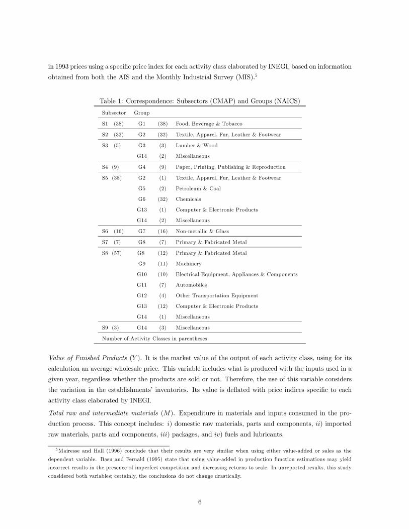
The description and correspondence between both classifications are detailed in Table 1, which
presents: i) the 9 CMAP subsectors, ii) the 14 NAICS groups, and iii) how the 9 CMAP subsectors have
been reorganised into the 14 NAICS groups. For instance, subsector 3, Lumber & Wood, contains five
activity classes (the numbers in parentheses in Table 1); these same five activity classes are reclassified
into two NAICS groups, G3 Lumber & Wood and G14 Miscellaneous, with three activity classes going to
G3 and the two remaining ones going to G14. Information on the main activities and products in each
group can be found in the Appendix.
The variables considered in this study are4
Output
Gross Value Added (V A) . The proxy for this variable is the difference between the value of finished
products (Y ) and the expenditure in intermediate materials (M). The series are deflated to be expressed
1The construction of the variables followed OECD (2001).2 It is important to note that despite the number of establishments, the AIS sample is somehow biased towards relatively
large establishments: more than a hundred employees, with a few exceptions.3We do not consider the crisis period 1994-1995 as this could bias our results.4 Similar results, unreported, are reached when other variables and methodologies for employment, capital and output
(i.e. number of workers, value of finished products, etc.) are considered. The decision to focus on the ones described in this
section is to facilitate comparisons with related studies.
5
in 1993 prices using a specific price index for each activity class elaborated by INEGI, based on information
obtained from both the AIS and the Monthly Industrial Survey (MIS).5
Table 1: Correspondence: Subsectors (CMAP) and Groups (NAICS)
Subsector Group
S1 (38) G1 (38) Food, Beverage & Tobacco
S2 (32) G2 (32) Textile, Apparel, Fur, Leather & Footwear
S3 (5) G3 (3) Lumber & Wood
G14 (2) Miscellaneous
S4 (9) G4 (9) Paper, Printing, Publishing & Reproduction
S5 (38) G2 (1) Textile, Apparel, Fur, Leather & Footwear
G5 (2) Petroleum & Coal
G6 (32) Chemicals
G13 (1) Computer & Electronic Products
G14 (2) Miscellaneous
S6 (16) G7 (16) Non-metallic & Glass
S7 (7) G8 (7) Primary & Fabricated Metal
S8 (57) G8 (12) Primary & Fabricated Metal
G9 (11) Machinery
G10 (10) Electrical Equipment, Appliances & Components
G11 (7) Automobiles
G12 (4) Other Transportation Equipment
G13 (12) Computer & Electronic Products
G14 (1) Miscellaneous
S9 (3) G14 (3) Miscellaneous
Number of Activity Classes in parentheses
Value of Finished Products (Y ). It is the market value of the output of each activity class, using for its
calculation an average wholesale price. This variable includes what is produced with the inputs used in a
given year, regardless whether the products are sold or not. Therefore, the use of this variable considers
the variation in the establishments’ inventories. Its value is deflated with price indices specific to each
activity class elaborated by INEGI.
Total raw and intermediate materials (M). Expenditure in materials and inputs consumed in the pro-
duction process. This concept includes: i) domestic raw materials, parts and components, ii) imported
raw materials, parts and components, iii) packages, and iv) fuels and lubricants.
5Mairesse and Hall (1996) conclude that their results are very similar when using either value-added or sales as the
dependent variable. Basu and Fernald (1995) state that using value-added in production function estimations may yield
incorrect results in the presence of imperfect competition and increasing returns to scale. In unreported results, this study
considered both variables; certainly, the conclusions do not change drastically.
6
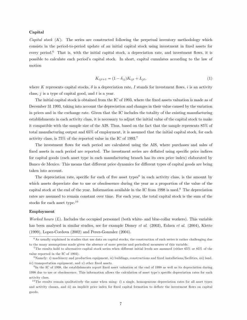
Capital
Capital stock (K). The series are constructed following the perpetual inventory methodology which
consists in the period-to-period update of an initial capital stock using investment in fixed assets for
every period.6 That is, with the initial capital stock, a depreciation rate, and investment flows, it is
possible to calculate each period’s capital stock. In short, capital cumulates according to the law of
motion
Kijt+1 = (1− δij)Kijt + Iijt, (1)
where K represents capital stocks, δ is a depreciation rate, I stands for investment flows, i is an activity
class, j is a type of capital good, and t is a year.
The initial capital stock is obtained from the IC of 1993, where the fixed assets valuation is made as of
December 31 1993, taking into account the depreciation and changes in their value caused by the variation
in prices and in the exchange rate. Given that the IC includes the totality of the existing manufacturing
establishments in each activity class, it is necessary to adjust the initial value of the capital stock to make
it compatible with the sample size of the AIS. Thus, based on the fact that the sample represents 85% of
total manufacturing output and 65% of employment, it is assumed that the initial capital stock, for each
activity class, is 75% of the reported value in the IC of 1993.7
The investment flows for each period are calculated using the AIS, where purchases and sales of
fixed assets in each period are reported. The investment series are deflated using specific price indices
for capital goods (each asset type in each manufacturing branch has its own price index) elaborated by
Banco de Mexico. This means that different price dynamics for different types of capital goods are being
taken into account.
The depreciation rate, specific for each of five asset types8 in each activity class, is the amount by
which assets depreciate due to use or obsolescence during the year as a proportion of the value of the
capital stock at the end of the year. Information available in the IC from 1998 is used.9 The depreciation
rates are assumed to remain constant over time. For each year, the total capital stock is the sum of the
stocks for each asset type.10
Employment
Worked hours (L). Includes the occupied personnel (both white- and blue-collar workers). This variable
has been analysed in similar studies, see for example Disney et al. (2003), Eslava et al. (2004), Klette
(1999), Lopez-Cordova (2002) and Perez-Gonzalez (2004).
6As usually explained in studies that use data on capital stocks, the construction of such series is rather challenging due
to the many assumptions made given the absence of more precise and periodical measures of this variable.7The results hold to alternative capital stock series when different initial levels are assumed (either 65% or 85% of the
value reported in the IC of 1993).8Namely: i) machinery and production equipment, ii) buildings, constructions and fixed installations/facilities, iii) land,
iv) transportation equipment, and v) other fixed assets.9 In the IC of 1998, the establishments report fixed asset valuation at the end of 1998 as well as its depreciation during
1998 due to use or obsolescence. This information allows the calculation of asset type’s specific depreciation rates for each
activity class.10The results remain qualitatively the same when using: i) a single, homogeneous depreciation rates for all asset types
and activity classes, and ii) an implicit price index for fixed capital formation to deflate the investment flows on capital
goods.
7
Worked hours adjusted by quality (Ladj). Total amount of hours worked by the occupied personnel (L)
multiplied by the wage per hour in the activity class as ratio of the wage per hour in total manufacturing.11
Energy
Electricity (E). Value of the electricity consumed by manufacturing establishments in the production
process reported for each activity class in the AIS. To deflate the series, an electric energy specific index
is constructed as a weighted average of the specific price indices from the Producer Price Index (PPI)
of industrial electric energy elaborated by Banco de Mexico. The inclusion of energy consumption as
an input of production has been explored in several studies, see for instance Casacuberta et al. (2004),
Eslava et al. (2004) and Klette (1999).12
Transport
Transport (T ). Expenditure on transportation of manufactured products reported in the AIS is used.
The series are deflated using a transportation specific price index, which is calculated as a weighted
average of different transportation indices elaborated by Banco de Mexico from PPI. These indices are
aggregated using the generic goods’ weights in the PPI.13
3.1 Some Considerations
As most micro-empirical studies, this document faces some limitations, which are commented next.
First, we do not have establishments, firms or companies as a unit of study. Instead, each data point
corresponds to an “activity class”, that conglomerates a number of manufacturing establishments into it.
Implicitly, this is assuming that every establishment in each activity class is somehow alike in terms of
its manufacturing processes, technology, etc.
Second, the time horizon considered in this study is relatively short (8 years, from 1996 to 2003),
which may impede to observe a complete economic cycle and thus bias our productivity estimates. For
example, it is worth mentioning the sharp fall in the Automobile sector’s output in some of the years of
the sample, an issue that, in this study, would imply a decrease in productivity.
Third, the construction of variables may suffer from the typical problems in measurement and con-
struction of variables (i.e. simple models of depreciation, lack of data, use of proxies for variables, deflated
variables with ‘general’ price indices, etc.). For example: i) the variable of capital aggregates different
types of investment in different years using simple models of depreciation. This is a common practice in
similar studies and it may yield biases, and ii) V A is deflated by specific price indices for each activity
class; however, the majority of the establishments manufacture more than a single and homogeneous
product, that is, one price index is considered for different establishments with different product ranges
in the same activity class.
11Group’s wages per hour are calculated as the weighted average of wages per hour in the activity classes corresponding
to each group, using worked hours as weights. The same procedure is followed for the calculation of wages per hour in the
whole sector.12Consumption (thousands of Kw/h) could have been used as well. However, there are many zeroes reported in 1998 and
2003.13The generics used for the calculation of this specific index are: i) railroad cargo transportation, ii) general automotive
cargo transportation, iii) sea cargo transportation, and iv) air cargo transportation.
8
Fifth, more precise calculations and estimates could be obtained if additional information were avail-
able, particularly about: i) the composition of worked hours (schooling and training levels, productive
process incidence, etc.), ii) the capital stock (asset lifetime, energy efficiency, technological level, training
required for its operation, etc.), iii) the use of and expenditure in telecommunications, and iv) the main
type of transportation used (by air, rail, road or sea) and destination (distance) of their products.
Finally, on the econometric side, due to the few observations available in some manufacturing subsec-
tors/groups, one must be cautious with the obtained production function estimates.
4 Characteristics of Mexican Manufacturing: 1996-2003
This section is divided into two parts. First, we briefly analyse different dimensions such as output share
composition, export orientation, concentration and technology adoption of the Mexican manufacturing
industry. Second, we focus on LP, human capital intensity and labour mobility.
4.1 Some Characteristics
Composition
Regarding the composition of output amongst the different groups in Mexican manufacturing, in 2003
the groups with a large share in total output were G11 Automobiles (15.8%), G6 Chemicals (15.5%) and
G8 Primary & Fabricated Metal (11.0%), whilst the lowest shares were for G3 Lumber & Wood (0.3%),
G5 Petroleum & Coal (0.6%) and G14 Miscellaneous (1.0%), see Table A1 in the Appendix.14
Also, the change in composition, between 1996 and 2003, is shown for each group. In this regard, it
is observed that G13 Computer & Electronic Products is the only group that has considerably increased
its share, by moving from 3.7% in 1996 to 8.6% in 2003 (4.9 p.p.). Contrasting with this case, the three
groups that presented the greatest decreases are G2 Textile, Apparel, Fur, Leather & Footwear (-1.5
p.p.), G6 Chemicals (-1.5 p.p.) and G8 Primary & Fabricated Metal (-1.3 p.p.).
Export Orientation
With respect to export orientation, the 14 groups in Mexican manufacturing show some differing patterns,
see Table A2 in the Appendix. This measure is equal to the ratio of exports to total sales. In 2003, this
ratio was between 2.4% for G5 Petroleum & Coal and 79% for G13 Computer & Electronic Products.
It is noteworthy that only 3 out of 14 groups have shown an increase in their export orientation: G13
Computer & Electronic Products (+7.1 p.p.), G10 Electrical Equipment, Appliances & Components
(+6.5 p.p.) and G9 Machinery (+3.6 p.p.). The whole sector has shown a decrease of 1.8 p.p. in this
measure by moving from 29.4% in 1996 to 27.6% in 2003. Effectively, and in spite of the period under
consideration, G11 Automobiles and G13 Computer & Electronic Products are clear exporting groups.
Concentration
The market structure of Mexican manufacturing is studied based on Herfindahl-Hirschman (HH) concen-
tration indices calculated for each of the 14 groups.15 In general, concentration has increased between
1996 and 2003 amongst the diverse groups of the sector, see Table A3 in the Appendix. Concentration14Table A1 also includes the share based on worked hours.15The index is calculated as the sum of the squares of the market share held by the establishments pertaining to each group.
9
went up in 10 out of 14 groups, except in G13 Computer & Electronic Products, G9 Machinery, G8
Primary & Fabricated Metal and G4 Paper, Printing, Publishing & Reproduction.16 When considering
the concentration indices obtained for the activity classes corresponding to each group, it is observed that
between 1996 and 2003 the minimum value of the HH index increased in 12 of the 14 groups. Concentra-
tion increased in 149 out of 205 activity classes between 1996 and 2003; moreover, in 1996 there were 72
activity classes highly concentrated (i.e. HH>1,800), in 2003 the number increased to 90 activity classes.
Technology Adoption
Measured as the expenditure in technology transfers and royalties as a proportion of V A. The variable
includes concepts such as patents and trademarks, technical consulting, basic engineering, services in
administrative technology and business operation.17 This measure can be understood as a proxy for by
innovation and technology related activities. For simplicity, henceforth we will refer to it as ‘technology
adoption’.
The groups in the top three positions of the ranking are G13 Computer & Electronic Products, G6
Chemicals and G10 Electrical Equipment, Appliances & Components. The groups in the last three
positions are G12 Other Transportation Equipment, G8 Primary & Fabricated Metal and G3 Lumber &
Wood, see Table A4 in the Appendix.
4.2 Labour Productivity, Human Capital Intensity and Labour Mobility
Labour Productivity (LP) is defined as V A per worked hour. Table 2 shows the levels of this variable
in 1996, 1999 and 2003, as well as its annual average growth rate during 1996-2003. G13 Computer &
Electronic Products and G5 Petroleum & Coal are the groups presenting the highest average growth
rates, whilst G9 Machinery and G12 Other Transportation Equipment the lowest ones.
To proxy for by the quality and the skill level of labour hired by the different manufacturing groups,
we construct the variable Human Capital Intensity. It is equal to labour remunerations per worked
hour paid in each manufacturing group divided by the weighted average labour remunerations paid in
the whole sector (i.e. relative wage).18 G5 Petroleum & Coal shows the greatest intensity in human
capital, followed by G6 Chemicals, G11 Automobiles, and G13 Computer & Electronic Products. At the
bottom of the ranking are G3 Lumber & Wood, G2 Textiles and G14 Miscellaneous, see Table A5 in the
Appendix. This could be reflecting differences in the quality of human capital required by each group,
as well as the possibility that some unions obtain additional benefits due to their bargaining power (rent
extraction).
Its value ranges between 0 and 10,000, the latter being the case of monopoly. The index is given by HHjt =Ji=1 (MSijt)
2
with MSijt = Yijt/Ji=1 Yijt, where MS is market share (in percent, from 0 to 100); and i is an establishment in group j
at time t. HH indices are reported for activity classes as well, see Table A3 in the Appendix. The HH indices are calculated
according to the shares in the value of finished products.16 It is important to note that the indices are calculated on the basis of the establishments considered in the AIS sample,
that is, other issues such as imports competing with domestically produced goods or the competition faced by domestic
firms in international markets, are not explicitly taken into account in the construction of the index.17 It does not include purchase of patents and trademarks.18Differences in Human Capital Intensity might be related to the observed differentials in LP amongst manufacturing
groups.
10
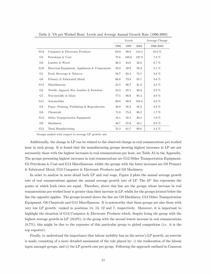
Table 2: VA per Worked Hour: Levels and Average Annual Growth Rate (1996-2003)
Levels Average Change
1996 1999 2003 1996-2003
G13 Computer & Electronic Products 63.9 80.0 124.4 10.0 %
G5 Petroleum & Coal 75.6 100.6 127.9 7.8 %
G3 Lumber & Wood 20.3 24.8 32.0 6.7 %
G10 Electrical Equipment, Appliances & Components 42.0 49.9 59.4 5.1 %
G1 Food, Beverage & Tobacco 56.7 65.4 73.7 3.8 %
G8 Primary & Fabricated Metal 66.8 73.9 85.7 3.6 %
G14 Miscellaneous 24.5 26.7 31.3 3.5 %
G2 Textile, Apparel, Fur, Leather & Footwear 24.5 25.1 30.2 3.0 %
G7 Non-metallic & Glass 77.5 86.0 95.4 3.0 %
G11 Automobiles 86.0 90.9 104.4 2.8 %
G4 Paper, Printing, Publishing & Reproduction 48.0 56.3 58.2 2.8 %
G6 Chemicals 71.0 75.8 80.2 1.7 %
G12 Other Transportation Equipment 19.1 28.1 20.4 1.0 %
G9 Machinery 40.7 37.6 43.1 0.8 %
G15 Total Manufacturing 55.3 61.7 69.8 3.4 %
Groups ranked with respect to average LP growth rate
Additionally, the change in LP can be related to the observed change in real remunerations per worked
hour in each group. It is found that the manufacturing groups showing highest increases in LP are not
necessarily those with the highest increases in real remunerations per hour, see Table A5 in the Appendix.
The groups presenting highest increases in real remunerations are G12 Other Transportation Equipment,
G5 Petroleum & Coal and G14 Miscellaneous; whilst the groups with the lower increases are G8 Primary
& Fabricated Metal, G13 Computer & Electronic Products and G9 Machinery.
In order to analyse in more detail both LP and real wage, Figure 2 plots the annual average growth
rate of real remunerations against the annual average growth rate of LP. The 45◦ line represents the
points at which both rates are equal. Therefore, above this line are the groups whose increase in real
remunerations per worked hour is greater than their increase in LP, whilst for the groups located below the
line the opposite applies. The groups located above the line are G9 Machinery, G12 Other Transportation
Equipment, G6 Chemicals and G14 Miscellaneous. It is noteworthy that these groups are also those with
very low LP growth: ranked in positions 14, 13, 12 and 7, respectively. Moreover, it is important to
highlight the situation of G13 Computer & Electronic Products which, despite being the group with the
highest average growth in LP (10.0%), is the group with the second lowest increase in real remunerations
(0.7%); this might be due to the exposure of this particular group to global competition (i.e. it is the
top exporter).
Finally, to understand the importance that labour mobility has on the sector’s LP growth, an exercise
is made, consisting of a more detailed assessment of the role played by: i) the reallocation of the labour
input amongst groups, and ii) the LP growth rate per group. Following the approach outlined in Cameron
11
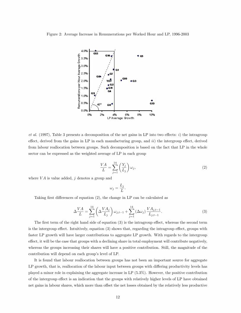
Figure 2: Average Increase in Remunerations per Worked Hour and LP, 1996-2003
et al. (1997), Table 3 presents a decomposition of the net gains in LP into two effects: i) the intragroup
effect, derived from the gains in LP in each manufacturing group, and ii) the intergroup effect, derived
from labour reallocation between groups. Such decomposition is based on the fact that LP in the whole
sector can be expressed as the weighted average of LP in each group
V A
L=
14Xj=1
µYjLj
¶ωj , (2)
where V A is value added, j denotes a group and
ωj =LjL.
Taking first differences of equation (2), the change in LP can be calculated as
∆V A
L=
14Xj=1
µ∆V Aj
Lj
¶ωj,t−1 +
14Xj=1
(∆ωj)V Aj,t−1Lj,t−1
. (3)
The first term of the right hand side of equation (3) is the intragroup effect, whereas the second term
is the intergroup effect. Intuitively, equation (3) shows that, regarding the intragroup effect, groups with
faster LP growth will have larger contributions to aggregate LP growth. With regards to the intergroup
effect, it will be the case that groups with a declining share in total employment will contribute negatively,
whereas the groups increasing their shares will have a positive contribution. Still, the magnitude of the
contribution will depend on each group’s level of LP.
It is found that labour reallocation between groups has not been an important source for aggregate
LP growth, that is, reallocation of the labour input between groups with differing productivity levels has
played a minor role in explaining the aggregate increase in LP (5.3%). However, the positive contribution
of the intergroup effect is an indication that the groups with relatively higher levels of LP have obtained
net gains in labour shares, which more than offset the net losses obtained by the relatively less productive
12
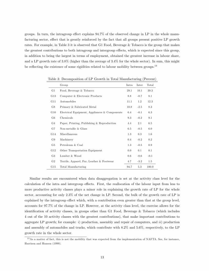
groups. In turn, the intragroup effect explains 94.7% of the observed change in LP in the whole manu-
facturing sector, effect that is greatly reinforced by the fact that all groups present positive LP growth
rates. For example, in Table 3 it is observed that G1 Food, Beverage & Tobacco is the group that makes
the greatest contributions to both intragroup and intergroup effects, which is expected since this group,
in addition to being the largest in terms of employment, obtained the greatest increase in labour share,
and a LP growth rate of 3.8% (higher than the average of 3.4% for the whole sector). In sum, this might
be reflecting the existence of some rigidities related to labour mobility between groups.19
Table 3: Decomposition of LP Growth in Total Manufacturing (Percent)
Group Intra Inter Total
G1 Food, Beverage & Tobacco 29.1 10.1 39.3
G13 Computer & Electronic Products 8.8 -0.7 8.1
G11 Automobiles 11.1 1.2 12.3
G8 Primary & Fabricated Metal 10.8 -2.5 8.3
G10 Electrical Equipment, Appliances & Components 6.4 -0.1 6.3
G6 Chemicals 9.3 -0.2 9.1
G4 Paper, Printing, Publishing & Reproduction 4.4 2.1 6.5
G7 Non-metallic & Glass 6.5 -0.5 6.0
G14 Miscellaneous 1.3 0.3 1.6
G9 Machinery 0.4 -0.2 0.2
G5 Petroleum & Coal 1.3 -0.5 0.9
G12 Other Transportation Equipment 0.0 0.1 0.1
G3 Lumber & Wood 0.6 -0.6 -0.1
G2 Textile, Apparel, Fur, Leather & Footwear 4.7 -3.2 1.5
G15 Total Manufacturing 94.7 5.3 100.0
Similar results are encountered when data disaggregation is set at the activity class level for the
calculation of the intra and intergroup effects. First, the reallocation of the labour input from less to
more productive activity classes plays a minor role in explaining the growth rate of LP for the whole
sector, accounting for only 2.3% of the net change in LP. Second, the bulk of the growth rate of LP is
explained by the intragroup effect which, with a contribution even greater than that at the group level,
accounts for 97.7% of the change in LP. However, at the activity class level, the exercise allows for the
identification of activity classes, in groups other than G1 Food, Beverage & Tobacco (which includes
4 out of the 10 activity classes with the greatest contributions), that make important contributions to
aggregate LP growth; for example: i) production, assembly and repair of computers, and ii) production
and assembly of automobiles and trucks, which contribute with 8.2% and 5.6%, respectively, to the LP
growth rate in the whole sector.
19As a matter of fact, this is not the mobility that was expected from the implementation of NAFTA. See, for instance,
Harrison and Hanson (1999).
13

5 Methodology and Results
This section explains both the methodological approach undertaken to estimate the production functions
and to analyse some of the determinants of productivity, and presents the corresponding results.
5.1 Production Function
A Cobb-Douglas production function-type is assumed
Yit = AitKαiit L
βiit ; i = 1, . . . , N ; t = 1, . . . , T, (4)
where Y is a measure of output (V A in our case), A is a productivity parameter, K is capital and L
is labour, α and β are the output elasticities with respect to their corresponding factor, i is an activity
class and t is time.
In addition to the traditional calculation of α and β, other factor elasticities are calculated and
estimated, that is, different production functions, with electricity (E) and transport (T ), are considered.
Hence, the more general production function is given by
Yit = AitKαiit L
βiit E
γiit T
λiit . (5)
This approach is applied for the whole manufacturing sector and for the 14 groups.
5.1.1 Growth Accounting
To obtain the level of MFP, from (4) or the more general production function (5), we solve for A, which
can be calculated for each year
Ait =Yit
Kαiit L
βiit
.
The output elasticities of factors are approximated by the share of the input in the total cost assuming
constant returns to scale (CRS) and perfect competition. Therefore, the considered shares are specific
for each combination of inputs. The weighted average of the input shares is obtained for every activity
class corresponding to each group in the period 1996-2003.
A complementary approach consists on the calculation and comparison of growth rates. Besides the
changes in MFP, changes in the utilisation of inputs also explain the observed output growth. Specifically,
the contribution of each input to the average growth rate of output is equal to the average growth rate
of each input times its elasticity, that is
M %Yit =M %Ait + αi M %Kit + βi M %Lit.
Results
Total Sector
Table 4 presents the MFP growth rates, the factor shares and their respective contributions to the
observed average growth rate of value added for the whole sector. The output elasticity of capital is
between 0.28 (with KLET ) and 0.34 (with KL), whilst the elasticity of labour is between 0.56 (with
14
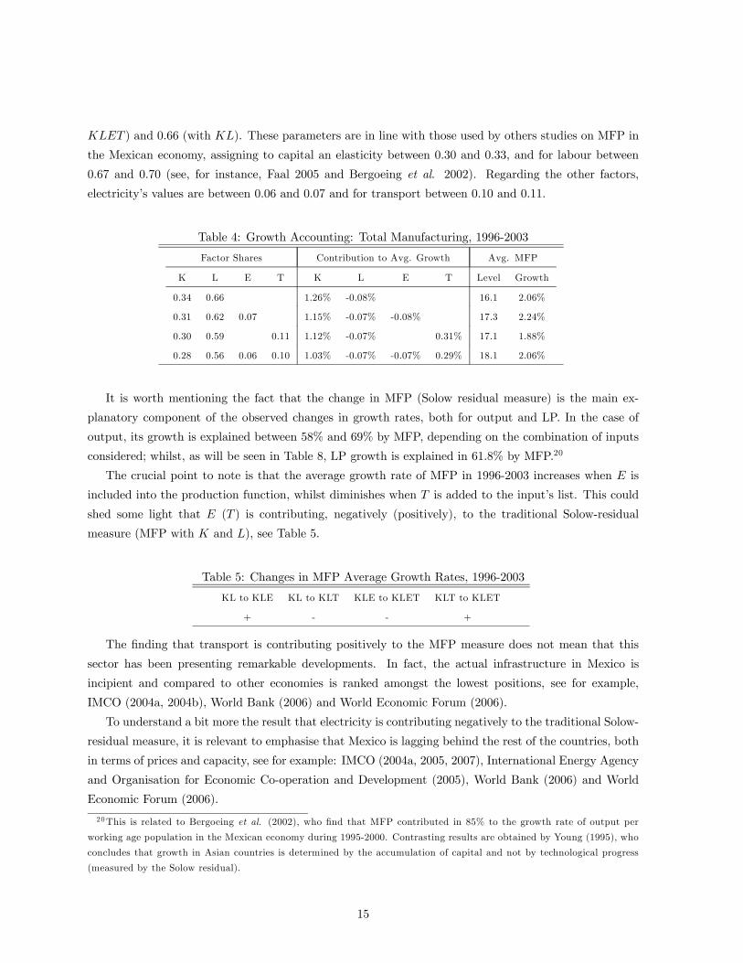
KLET ) and 0.66 (with KL). These parameters are in line with those used by others studies on MFP in
the Mexican economy, assigning to capital an elasticity between 0.30 and 0.33, and for labour between
0.67 and 0.70 (see, for instance, Faal 2005 and Bergoeing et al. 2002). Regarding the other factors,
electricity’s values are between 0.06 and 0.07 and for transport between 0.10 and 0.11.
Table 4: Growth Accounting: Total Manufacturing, 1996-2003
Factor Shares Contribution to Avg. Growth Avg. MFP
K L E T K L E T Level Growth
0.34 0.66 1.26% -0.08% 16.1 2.06%
0.31 0.62 0.07 1.15% -0.07% -0.08% 17.3 2.24%
0.30 0.59 0.11 1.12% -0.07% 0.31% 17.1 1.88%
0.28 0.56 0.06 0.10 1.03% -0.07% -0.07% 0.29% 18.1 2.06%
It is worth mentioning the fact that the change in MFP (Solow residual measure) is the main ex-
planatory component of the observed changes in growth rates, both for output and LP. In the case of
output, its growth is explained between 58% and 69% by MFP, depending on the combination of inputs
considered; whilst, as will be seen in Table 8, LP growth is explained in 61.8% by MFP.20
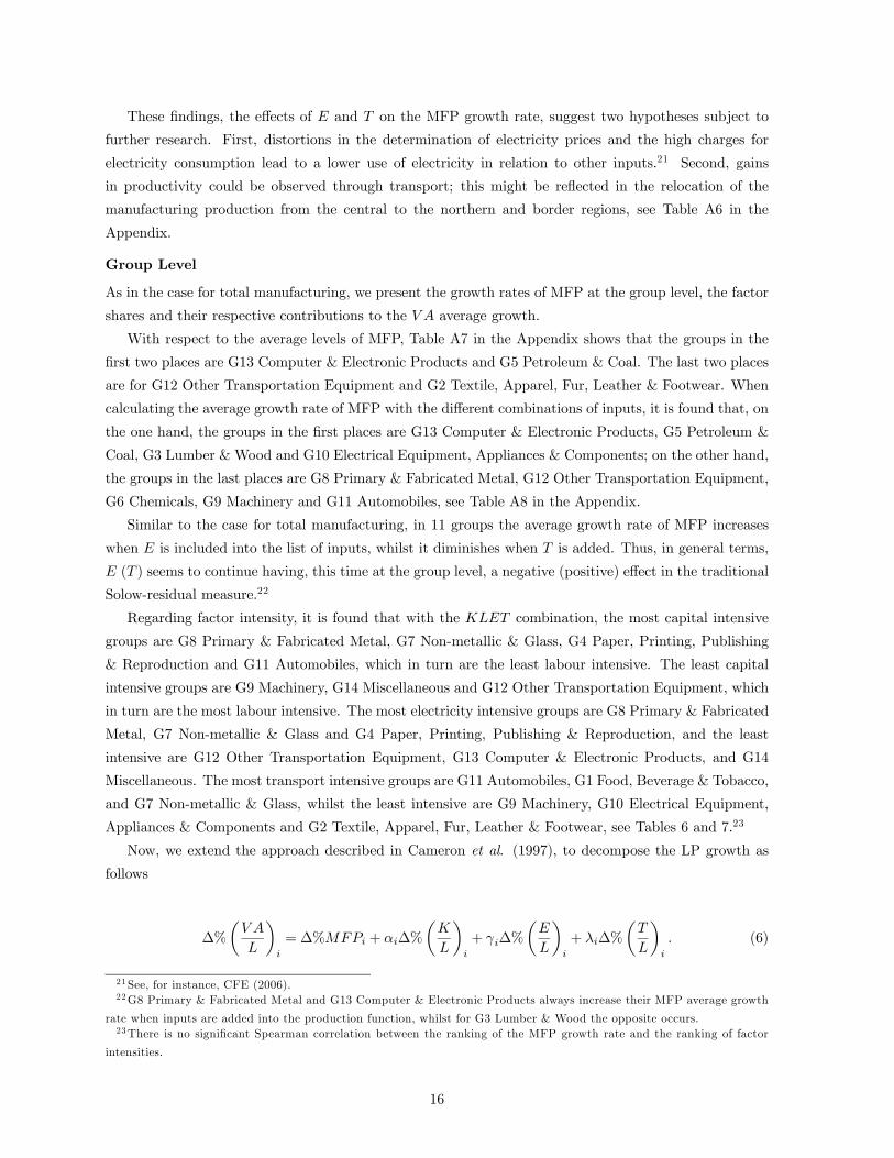
The crucial point to note is that the average growth rate of MFP in 1996-2003 increases when E is
included into the production function, whilst diminishes when T is added to the input’s list. This could
shed some light that E (T ) is contributing, negatively (positively), to the traditional Solow-residual
measure (MFP with K and L), see Table 5.
Table 5: Changes in MFP Average Growth Rates, 1996-2003
KL to KLE KL to KLT KLE to KLET KLT to KLET
+ - - +
The finding that transport is contributing positively to the MFP measure does not mean that this
sector has been presenting remarkable developments. In fact, the actual infrastructure in Mexico is
incipient and compared to other economies is ranked amongst the lowest positions, see for example,
IMCO (2004a, 2004b), World Bank (2006) and World Economic Forum (2006).
To understand a bit more the result that electricity is contributing negatively to the traditional Solow-
residual measure, it is relevant to emphasise that Mexico is lagging behind the rest of the countries, both
in terms of prices and capacity, see for example: IMCO (2004a, 2005, 2007), International Energy Agency
and Organisation for Economic Co-operation and Development (2005), World Bank (2006) and World
Economic Forum (2006).
20This is related to Bergoeing et al. (2002), who find that MFP contributed in 85% to the growth rate of output per
working age population in the Mexican economy during 1995-2000. Contrasting results are obtained by Young (1995), who
concludes that growth in Asian countries is determined by the accumulation of capital and not by technological progress
(measured by the Solow residual).
15
These findings, the effects of E and T on the MFP growth rate, suggest two hypotheses subject to
further research. First, distortions in the determination of electricity prices and the high charges for
electricity consumption lead to a lower use of electricity in relation to other inputs.21 Second, gains
in productivity could be observed through transport; this might be reflected in the relocation of the
manufacturing production from the central to the northern and border regions, see Table A6 in the
Appendix.
Group Level
As in the case for total manufacturing, we present the growth rates of MFP at the group level, the factor
shares and their respective contributions to the V A average growth.
With respect to the average levels of MFP, Table A7 in the Appendix shows that the groups in the
first two places are G13 Computer & Electronic Products and G5 Petroleum & Coal. The last two places
are for G12 Other Transportation Equipment and G2 Textile, Apparel, Fur, Leather & Footwear. When
calculating the average growth rate of MFP with the different combinations of inputs, it is found that, on
the one hand, the groups in the first places are G13 Computer & Electronic Products, G5 Petroleum &
Coal, G3 Lumber & Wood and G10 Electrical Equipment, Appliances & Components; on the other hand,
the groups in the last places are G8 Primary & Fabricated Metal, G12 Other Transportation Equipment,
G6 Chemicals, G9 Machinery and G11 Automobiles, see Table A8 in the Appendix.
Similar to the case for total manufacturing, in 11 groups the average growth rate of MFP increases
when E is included into the list of inputs, whilst it diminishes when T is added. Thus, in general terms,
E (T ) seems to continue having, this time at the group level, a negative (positive) effect in the traditional
Solow-residual measure.22
Regarding factor intensity, it is found that with the KLET combination, the most capital intensive
groups are G8 Primary & Fabricated Metal, G7 Non-metallic & Glass, G4 Paper, Printing, Publishing
& Reproduction and G11 Automobiles, which in turn are the least labour intensive. The least capital
intensive groups are G9 Machinery, G14 Miscellaneous and G12 Other Transportation Equipment, which
in turn are the most labour intensive. The most electricity intensive groups are G8 Primary & Fabricated
Metal, G7 Non-metallic & Glass and G4 Paper, Printing, Publishing & Reproduction, and the least
intensive are G12 Other Transportation Equipment, G13 Computer & Electronic Products, and G14
Miscellaneous. The most transport intensive groups are G11 Automobiles, G1 Food, Beverage & Tobacco,
and G7 Non-metallic & Glass, whilst the least intensive are G9 Machinery, G10 Electrical Equipment,
Appliances & Components and G2 Textile, Apparel, Fur, Leather & Footwear, see Tables 6 and 7.23
Now, we extend the approach described in Cameron et al. (1997), to decompose the LP growth as
follows
∆%
µV A
L
¶i
= ∆%MFPi + αi∆%
µK
L
¶i
+ γi∆%
µE
L
¶i
+ λi∆%
µT
L
¶i
. (6)
21See, for instance, CFE (2006).22G8 Primary & Fabricated Metal and G13 Computer & Electronic Products always increase their MFP average growth
rate when inputs are added into the production function, whilst for G3 Lumber & Wood the opposite occurs.23There is no significant Spearman correlation between the ranking of the MFP growth rate and the ranking of factor
intensities.
16
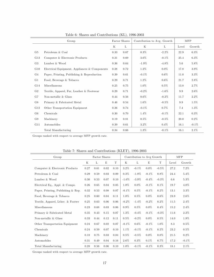
Table 6: Shares and Contributions (KL), 1996-2003
Group Factor Shares Contribution to Avg. Growth MFP
K L K L Level Growth
G5 Petroleum & Coal 0.33 0.67 0.3% -2.2% 22.9 6.3%
G13 Computer & Electronic Products 0.31 0.69 3.6% -0.1% 25.4 6.3%
G3 Lumber & Wood 0.36 0.64 -1.9% -4.8% 5.6 5.8%
G10 Electrical Equipment, Appliances & Components 0.28 0.72 1.2% 0.0% 17.8 3.9%
G4 Paper, Printing, Publishing & Reproduction 0.39 0.61 -0.1% 0.6% 11.0 3.3%
G1 Food, Beverage & Tobacco 0.29 0.71 1.2% 0.6% 21.7 2.8%
G14 Miscellaneous 0.25 0.75 1.0% 0.5% 13.8 2.7%
G2 Textile, Apparel, Fur, Leather & Footwear 0.29 0.71 -0.2% -1.6% 9.9 2.6%
G7 Non-metallic & Glass 0.44 0.56 0.6% -0.2% 11.7 2.2%
G8 Primary & Fabricated Metal 0.46 0.54 1.6% -0.5% 9.9 1.5%
G12 Other Transportation Equipment 0.26 0.74 -0.1% 0.7% 7.4 1.3%
G6 Chemicals 0.30 0.70 1.4% -0.1% 22.1 0.3%
G9 Machinery 0.19 0.81 0.5% -0.5% 20.0 0.2%
G11 Automobiles 0.39 0.61 3.2% 0.4% 16.1 -0.1%
Total Manufacturing 0.34 0.66 1.3% -0.1% 16.1 2.1%
Groups ranked with respect to average MFP growth rate.
Table 7: Shares and Contributions (KLET), 1996-2003
Group Factor Shares Contribution to Avg Growth MFP
K L E T K L E T Level Growth
Computer & Electronic Products 0.27 0.61 0.02 0.10 3.2% -0.1% 0.0% -0.5% 27.2 7.2%
Petroleum & Coal 0.29 0.59 0.03 0.09 0.3% -1.9% -0.1% 0.8% 24.4 5.4%
Lumber & Wood 0.30 0.53 0.07 0.10 -1.6% -3.9% -0.4% -0.3% 6.6 5.3%
Electrical Eq., Appl. & Comps. 0.26 0.65 0.04 0.05 1.0% 0.0% -0.1% 0.1% 19.7 4.0%
Paper, Printing, Publishing & Rep. 0.32 0.53 0.08 0.07 -0.1% 0.5% -0.1% 0.2% 13.1 3.3%
Food, Beverage & Tobacco 0.25 0.60 0.04 0.11 1.0% 0.5% 0.0% 0.6% 23.9 2.6%
Textile, Apparel, Lther. & Footwr 0.25 0.63 0.06 0.06 -0.2% -1.4% -0.2% 0.2% 11.5 2.4%
Miscellaneous 0.23 0.68 0.03 0.06 0.9% 0.5% 0.0% 0.4% 15.2 2.4%
Primary & Fabricated Metal 0.35 0.43 0.15 0.07 1.3% -0.4% -0.1% -0.3% 11.6 2.2%
Non-metallic & Glass 0.33 0.44 0.12 0.11 0.5% -0.2% 0.0% 0.5% 14.0 1.9%
Other Transportation Equipment 0.24 0.67 0.02 0.07 -0.1% 0.6% -0.1% 1.0% 8.3 0.5%
Chemicals 0.24 0.59 0.07 0.10 1.1% -0.1% -0.1% 0.2% 23.2 0.5%
Machinery 0.18 0.75 0.03 0.04 0.5% -0.5% 0.0% 0.0% 21.5 0.2%
Automobiles 0.31 0.49 0.04 0.16 2.6% 0.3% 0.1% 0.7% 17.2 -0.1%
Total Manufacturing 0.28 0.56 0.06 0.10 1.0% -0.1% -0.1% 0.3% 18.1 2.1%
Groups ranked with respect to average MFP growth rate.
17

The decomposition consists of two parts: i) the change in MFP and ii) the change in inputs, capital,
electricity and transport per unit of labour (the last three terms of equation (6)). Table 8 shows that,
for total manufacturing, 61.8% of the increase in LP is explained by MFP growth. Capital accumulation
per unit of labour is the second most important component representing 32.4% of the observed increase
in LP. The use of electricity per unit of labour contributes negatively, close to 3%, of the change in LP.
The remaining 8.8% is explained by the increase in transport per unit of labour.
At the group level, it is observed, also from Table 8, that for the group with the major increase in LP,
G13 Computer & Electronic Products, MFP explains approximately 72%. The groups in which capital
accumulation explains most of the growth in LP are G11 Automobiles (84%), and G9 Machinery (74%).24
The change in the use of electricity per unit of labour has a negative effect in eight groups and almost
nil in three groups. The group in which the increase in the use of transport per unit of labour has a
greater impact on LP growth is G12 Other Transportation Equipment (94%). MFP plays a major role in
explaining LP growth in G4 Paper, Printing, Publishing & Reproduction (117%), G2 Textile, Apparel,
Leather, Fur, & Footwear (80%) and G10 Electrical Equipment, Appliances & Components (79%).
Table 8: Decomposition of Labour Productivity Growth Rate
Contribution Contribution (% of LP)
Group LP MFP αK/L γE/L λT/L MFP αK/L γE/L λT/L
Computer & Electronic Products 10.0 7.2 3.2 0.0 -0.5 72.3 32.0 0.2 -4.8
Petroleum & Coal 7.8 5.4 1.2 0.0 1.1 68.7 15.9 0.2 14.4
Lumber & Wood 6.7 5.3 0.7 0.2 0.4 79.5 10.5 2.6 6.6
Electrical Eq., Appl. & Comps. 5.1 4.0 1.1 -0.1 0.1 78.6 20.7 -2.5 2.8
Food, Beverage & Tobacco 3.8 2.6 0.8 -0.1 0.5 67.4 20.9 -1.6 13.0
Primary & Fabricated Metal 3.6 2.2 1.6 0.0 -0.2 60.6 44.4 0.6 -5.6
Miscellaneous 3.5 2.4 0.8 0.0 0.4 67.3 21.7 -0.6 11.4
Textile, Apparel, Lther. & Footwr 3.0 2.4 0.4 -0.1 0.3 79.6 12.0 -1.9 10.2
Non-metallic & Glass 3.0 1.9 0.6 0.0 0.5 62.2 20.1 0.2 17.1
Automobiles 2.8 -0.1 2.3 0.0 0.6 -4.0 83.5 1.3 21.1
Paper, Printing, Publishing & Rep. 2.8 3.3 -0.4 -0.1 0.1 116.8 -15.2 -5.1 4.2
Chemicals 1.7 0.5 1.2 -0.1 0.2 28.9 65.9 -7.8 14.1
Other Transportation Equipment 1.0 0.5 -0.3 -0.1 0.9 56.0 -28.0 -15.3 93.5
Machinery 0.8 0.2 0.6 0.0 0.1 21.8 73.9 -1.4 6.6
Total Manufacturing 3.4 2.1 1.1 -0.1 0.3 61.8 32.4 -2.9 8.8
Groups ranked with respect to average LP growth rate
Finally, Figure A1 in the Appendix shows the position of MFP levels of each group relative to the
24The fact that Automobiles shows the highest capital accumulation component is consistent with the fact that, as
mentioned in Banco de Mexico’s Inflation Report for January-March 2006, in the last few years most of the assembly plants
established in the country have made important investments to expand and modernise their production capacities (including
the construction of new plants).
18

average level of the manufacturing sector during 1996-2003. The literature mentions that increases in the
dispersion of relative MFP levels through time could be evidence that the development and/or adoption
of technology is very specific for some groups and is not being transmitted rapidly to others, see Cameron
et al. (1997). The dispersion of the relative levels of MFP has increased in Mexican manufacturing;
however, this is due exclusively to one group, G13 Computer & Electronic Products, which as mentioned
in subsection 4.1, occupies the first place in technology transfers and royalties (technology adoption).
Once this is taken into account (excluding G13 Computer & Electronic Products), it is found that the
dispersion has remained the same.
5.1.2 Econometric Estimation
Diverse econometric methods are considered to estimate the production functions. For total manufac-
turing, dynamic specifications are studied by means of a system GMM, following Blundell and Bond
(2000), and static specifications by means of Fixed Effects (FE, see Dwyer 1996) and Random Coeffi-
cients Method (RCM, see Biorn et al. 2002). Due to the reduced number of activity classes for most of
the 14 groups, the dynamic specification is not estimated to that level; hence, only static estimations are
considered.
In all estimations, logarithms are applied to (4)
yit = αkit + βlit + ait, (7)
where lower-case letters stand for the respective log-variables of the function. The residual, ait, is consid-
ered as a measure of MFP. Hence, with the estimated coefficients (α and β), growth accounting exercises,
similar to those described in subsection 5.1.1, are undertaken.
With respect to the system GMM, it is assumed that ait can be decomposed as
ait = ηi + ηt + uit, (8)
where ηi captures differences in productivity — specific for each activity class and fixed over time, ηtcaptures common time varying productivity shocks, and uit captures productivity shocks for each activity
class.
The static representation can be estimated by OLS and/or fixed effects as in similar studies; however,
there is evidence that uit is usually persistent over time, implying that the different activity classes do not
adjust instantaneously and/or the existence of omitted variable bias of a particular form (i.e. intangibles).
This issue can be taken into account by considering an autoregressive form, that is
uit = φuit−1 + eit; |φ| < 1, (9)
where eit is an idiosyncratic error term. This allows to obtain a dynamic representation of (7)25
yit = δ1yit−1 + δ2kit + δ3kit−1 + δ4lit + δ5lit−1 + ηi(1− φ) + (ηt − φηt−1) + eit (10)
25The lagged dependent variable is a way to capture the fact that when production factors change, it takes time to output,
and consequently MFP, to achieve a new long-run level.
19

where δ1 = φ; δ2 = α; δ3 = −φα; δ4 = β; δ5 = −φβ. With δ3 and δ5 being two non-linear (common
factor) restrictions. As stated in Blundell and Bond (2000), given consistent estimates of the unrestricted
parameter vector δ = (δ1, δ2, δ3, δ4, δ5) and var(δ), these restrictions can be tested and imposed using
minimum distance to obtain the restricted parameter vector (α, β, φ).
Results
Persistence
Before commenting on the estimation results, a word should be said about some of the characteristics
of our data. When the series are persistent, the instruments used for the difference GMM estimator
are weak, so this estimator would be inappropriate given the existence of such persistence.26 Therefore,
under that context, a more appropriate estimation would be achieved by means of a system GMM, see
Bond et al. (2005).
Hence, to better understand the results determined by the system GMM, a brief analysis of the series
is presented. Following Bond et al. (2005), unit root tests, based on OLS estimation of an AR(1) process,
are presented as it has been shown that such procedure has better power properties than alternative
panel unit root tests in the setting of a relatively large cross-section dimension and a small number of
time periods.
Table A9 in the Appendix presents tests of the unit root hypothesis for the first set of variables used
in the empirical part, being these: Y, V A, K, L, E and T . Table A10 in the Appendix presents a second
set of variables that will be considered in Section 5.2.1; these are: MFP , LP , intensities for K, E and
T , technology adoption, concentration, human capital intensity and exports.
Specifically, of all the studied variables, the null hypothesis of a unit root is not rejected only for
capital and transport when time dummies are included; once individual dummies are included, the null
is rejected for these two variables. The other variables show no evidence of a panel unit root. Still, they
present a relatively high degree of persistence. Other standard panel unit root tests for the series find no
evidence of a unit root.27 In short, the results show certain degree of persistence and, in few cases, close
to random walk processes.28 Then, this provides further validity to our system GMM estimation results.
Total Sector
With respect to the total manufacturing, using a panel of the 205 activity classes for the period
1996-2003, we focus first on the results based on the system GMM, which present a constant return to
scale (Wald) test (labeled as CRS) and a common factor test (labeled as Comfac)29 of the unrestricted
specification, see Table A11 in the Appendix. As can be seen, the test does not reject the null hypothesis
of CRS in the different specifications. Therefore, estimations imposing CRS are presented in Table A12
in the Appendix. It is important to mention that the system GMM is also used in section 5.2.1, where
further details of this estimator will be provided.26For instance, in the case of a random walk, there would not be correlation between the variables in first differences
and the lagged levels, this means that the autoregressive coefficient would not be identified, as the rank condition is not
satisfied; thus, the instruments would not add any information.27Unreported in the paper.28The system GMM estimator is preferred (based on both applied research and Monte Carlo simulations), when there
are highly persistent processes.29The test is a minimum distance test of the non-linear common factor restrictions imposed in the restricted models. The
null hypothesis is that the restrictions are adequate.
20
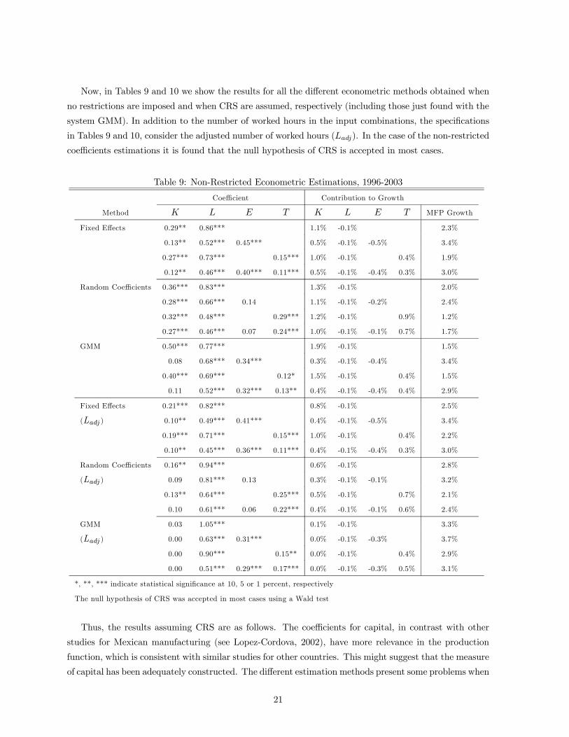
Now, in Tables 9 and 10 we show the results for all the different econometric methods obtained when
no restrictions are imposed and when CRS are assumed, respectively (including those just found with the
system GMM). In addition to the number of worked hours in the input combinations, the specifications
in Tables 9 and 10, consider the adjusted number of worked hours (Ladj). In the case of the non-restricted
coefficients estimations it is found that the null hypothesis of CRS is accepted in most cases.
Table 9: Non-Restricted Econometric Estimations, 1996-2003
Coefficient Contribution to Growth
Method K L E T K L E T MFP Growth
Fixed Effects 0.29** 0.86*** 1.1% -0.1% 2.3%
0.13** 0.52*** 0.45*** 0.5% -0.1% -0.5% 3.4%
0.27*** 0.73*** 0.15*** 1.0% -0.1% 0.4% 1.9%
0.12** 0.46*** 0.40*** 0.11*** 0.5% -0.1% -0.4% 0.3% 3.0%
Random Coefficients 0.36*** 0.83*** 1.3% -0.1% 2.0%
0.28*** 0.66*** 0.14 1.1% -0.1% -0.2% 2.4%
0.32*** 0.48*** 0.29*** 1.2% -0.1% 0.9% 1.2%
0.27*** 0.46*** 0.07 0.24*** 1.0% -0.1% -0.1% 0.7% 1.7%
GMM 0.50*** 0.77*** 1.9% -0.1% 1.5%
0.08 0.68*** 0.34*** 0.3% -0.1% -0.4% 3.4%
0.40*** 0.69*** 0.12* 1.5% -0.1% 0.4% 1.5%
0.11 0.52*** 0.32*** 0.13** 0.4% -0.1% -0.4% 0.4% 2.9%
Fixed Effects 0.21*** 0.82*** 0.8% -0.1% 2.5%
(Ladj ) 0.10** 0.49*** 0.41*** 0.4% -0.1% -0.5% 3.4%
0.19*** 0.71*** 0.15*** 1.0% -0.1% 0.4% 2.2%
0.10** 0.45*** 0.36*** 0.11*** 0.4% -0.1% -0.4% 0.3% 3.0%
Random Coefficients 0.16** 0.94*** 0.6% -0.1% 2.8%
(Ladj ) 0.09 0.81*** 0.13 0.3% -0.1% -0.1% 3.2%
0.13** 0.64*** 0.25*** 0.5% -0.1% 0.7% 2.1%
0.10 0.61*** 0.06 0.22*** 0.4% -0.1% -0.1% 0.6% 2.4%
GMM 0.03 1.05*** 0.1% -0.1% 3.3%
(Ladj ) 0.00 0.63*** 0.31*** 0.0% -0.1% -0.3% 3.7%
0.00 0.90*** 0.15** 0.0% -0.1% 0.4% 2.9%
0.00 0.51*** 0.29*** 0.17*** 0.0% -0.1% -0.3% 0.5% 3.1%
*, **, *** indicate statistical significance at 10, 5 or 1 percent, respectively
The null hypothesis of CRS was accepted in most cases using a Wald test
Thus, the results assuming CRS are as follows. The coefficients for capital, in contrast with other
studies for Mexican manufacturing (see Lopez-Cordova, 2002), have more relevance in the production
function, which is consistent with similar studies for other countries. This might suggest that the measure
of capital has been adequately constructed. The different estimation methods present some problems when
21
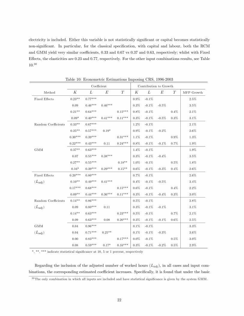
electricity is included. Either this variable is not statistically significant or capital becomes statistically
non-significant. In particular, for the classical specification, with capital and labour, both the RCM
and GMM yield very similar coefficients, 0.33 and 0.67 vs 0.37 and 0.63, respectively; whilst with Fixed
Effects, the elasticities are 0.23 and 0.77, respectively. For the other input combinations results, see Table
10.30
Table 10: Econometric Estimations Imposing CRS, 1996-2003
Coefficient Contribution to Growth
Method K L E T K L E T MFP Growth
Fixed Effects 0.23** 0.77*** 0.9% -0.1% 2.5%
0.09 0.46*** 0.46*** 0.3% -0.1% -0.5% 3.5%
0.21** 0.64*** 0.15*** 0.8% -0.1% 0.4% 2.1%
0.09* 0.40*** 0.41*** 0.11*** 0.3% -0.1% -0.5% 0.3% 3.1%
Random Coefficients 0.33** 0.67*** 1.2% -0.1% 2.1%
0.25** 0.57*** 0.19* 0.9% -0.1% -0.2% 2.6%
0.30*** 0.39*** 0.31*** 1.1% -0.1% 0.9% 1.3%
0.22*** 0.43*** 0.11 0.24*** 0.8% -0.1% -0.1% 0.7% 1.9%
GMM 0.37** 0.63*** 1.4% -0.1% 1.9%
0.07 0.55*** 0.38*** 0.3% -0.1% -0.4% 3.5%
0.27** 0.55*** 0.18** 1.0% -0.1% 0.5% 1.8%
0.16* 0.39*** 0.29*** 0.15** 0.6% -0.1% -0.3% 0.4% 2.6%
Fixed Effects 0.20*** 0.80*** 0.7% -0.1% 2.6%
(Ladj ) 0.10** 0.49*** 0.41*** 0.4% -0.1% -0.5% 3.4%
0.17*** 0.68*** 0.15*** 0.6% -0.1% 0.4% 2.2%
0.09** 0.44*** 0.36*** 0.11*** 0.3% -0.1% -0.4% 0.3% 3.0%
Random Coefficients 0.14** 0.86*** 0.5% -0.1% 2.8%
(Ladj ) 0.09 0.80*** 0.11 0.3% -0.1% -0.1% 3.1%
0.14** 0.63*** 0.23*** 0.5% -0.1% 0.7% 2.1%
0.09 0.63*** 0.08 0.20*** 0.3% -0.1% -0.1% 0.6% 2.5%
GMM 0.04 0.96*** 0.1% -0.1% 3.3%
(Ladj ) 0.04 0.71*** 0.25** 0.1% -0.1% -0.3% 3.6%
0.00 0.83*** 0.17*** 0.0% -0.1% 0.5% 3.0%
0.08 0.59*** 0.17* 0.16*** 0.3% -0.1% -0.2% 0.5% 2.9%
*, **, *** indicate statistical significance at 10, 5 or 1 percent, respectively
Regarding the inclusion of the adjusted number of worked hours (Ladj), in all cases and input com-
binations, the corresponding estimated coefficient increases. Specifically, it is found that under the basic
30The only combination in which all inputs are included and have statistical significance is given by the system GMM.
22
combination KL, 0.80 is the minimum elasticity for Ladj .31
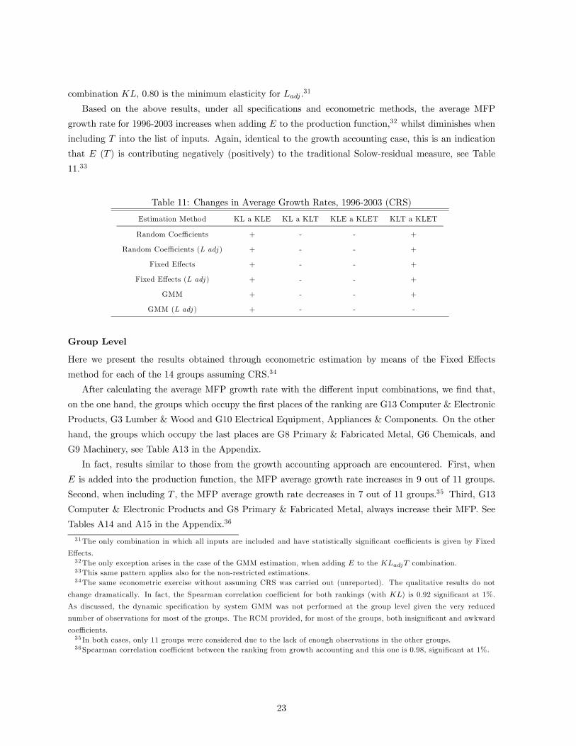
Based on the above results, under all specifications and econometric methods, the average MFP
growth rate for 1996-2003 increases when adding E to the production function,32 whilst diminishes when
including T into the list of inputs. Again, identical to the growth accounting case, this is an indication
that E (T ) is contributing negatively (positively) to the traditional Solow-residual measure, see Table
11.33
Table 11: Changes in Average Growth Rates, 1996-2003 (CRS)
Estimation Method KL a KLE KL a KLT KLE a KLET KLT a KLET
Random Coefficients + - - +
Random Coefficients (L adj ) + - - +
Fixed Effects + - - +
Fixed Effects (L adj ) + - - +
GMM + - - +
GMM (L adj ) + - - -
Group Level
Here we present the results obtained through econometric estimation by means of the Fixed Effects
method for each of the 14 groups assuming CRS.34
After calculating the average MFP growth rate with the different input combinations, we find that,
on the one hand, the groups which occupy the first places of the ranking are G13 Computer & Electronic
Products, G3 Lumber & Wood and G10 Electrical Equipment, Appliances & Components. On the other
hand, the groups which occupy the last places are G8 Primary & Fabricated Metal, G6 Chemicals, and
G9 Machinery, see Table A13 in the Appendix.
In fact, results similar to those from the growth accounting approach are encountered. First, when
E is added into the production function, the MFP average growth rate increases in 9 out of 11 groups.
Second, when including T , the MFP average growth rate decreases in 7 out of 11 groups.35 Third, G13
Computer & Electronic Products and G8 Primary & Fabricated Metal, always increase their MFP. See
Tables A14 and A15 in the Appendix.36
31The only combination in which all inputs are included and have statistically significant coefficients is given by Fixed
Effects.32The only exception arises in the case of the GMM estimation, when adding E to the KLadjT combination.33This same pattern applies also for the non-restricted estimations.34The same econometric exercise without assuming CRS was carried out (unreported). The qualitative results do not
change dramatically. In fact, the Spearman correlation coefficient for both rankings (with KL) is 0.92 significant at 1%.
As discussed, the dynamic specification by system GMM was not performed at the group level given the very reduced
number of observations for most of the groups. The RCM provided, for most of the groups, both insignificant and awkward
coefficients.35 In both cases, only 11 groups were considered due to the lack of enough observations in the other groups.36 Spearman correlation coefficient between the ranking from growth accounting and this one is 0.98, significant at 1%.
23
Estimations with Ladj
For completeness, we present the ranking of the groups under the different combinations of the production
functions obtained from econometric estimations for the 14 groups substituting L by Ladj and assuming
CRS.
Table A16 in the Appendix shows that there are no substantial differences with respect to the ranking
that does not present adjustments on the unit of labour.37 Again, G13 Computer & Electronic Products
is the group with the highest MFP growth. More interesting is to focus on the change that the estimated
coefficient (Ladj) experiences compared to the one obtained with L. On one hand, Table A17 in the
Appendix shows that G14 Miscellaneous, G13 Computer & Electronic Products, G7 Non-metallic &
Glass, and G10 Electrical Equipment, Appliances & Components are the groups which present the most
important positive changes. On the other hand, the groups that present the most important downwards
changes are G9 Machinery and G3 Lumber & Wood. These results seem to be consistent with what one
might expect: a more qualified labour force should prevail in groups such as G13 Computer & Electronic
Products than in groups such as G3 Lumber & Wood.
5.2 Determinants of MFP and LP
In this section, we use both a cross-section approach and a dynamic panel data approach with the intention
of identifying, econometrically, some possible determinants of productivity growth.
5.2.1 Econometric Estimation
Single cross-section productivity growth regressions (N = 205 activity classes, with averaged data for
1996-2003) are estimated as well as dynamic panel data regressions (N = 205 activity classes, t = 8
years).
For the static case, we consider the average growth rate for MFP (MMFP) and LP (MLP) as dependentvariables. The explanatory variables are the 1996-2003 averaged variables for factor intensities (K, E
and T ), concentration, technology adoption and exports.
It is important to bear in mind that when using cross-sectional regressions, one has to take into account
that: i) reducing time series to a single average observation means that not all available information is
being used, ii) it is likely that single cross-section regressions suffer from omitted variable bias, and iii)
one or more of the regressors may be endogenous. Moreover, since we are analysing growth of MFP and
LP and given the characteristics of the panel studied here (N large and T small), a dynamic panel data
estimation, using a system GMM, is a natural candidate to be considered. This type of estimation is able
to account for unobserved individual specific effects and allows for the endogeneity of one or more of the
regressors. In particular, the specification takes the following structure
pit = ω + θpit−1 + ψxit + ηi + ηt + vit, (11)
where p is the logarithm of either MFP or LP and xit is a vector of explanatory variables.
37When the labour input is not adjusted, the Spearman correlations between the rankings of MFP growth obtained by
means of growth accounting and econometric estimations (both restricted and non-restricted specifications) are very high,
above 0.90, and significant at the 1% level.
24
As demonstrated in Hsiao (2003), omitting unobserved time invariant individual effects in a dynamic
panel data model will cause OLS levels estimates to be biased and inconsistent, as the lagged dependent
variable is positively correlated with the permanent effects, ηi. An alternative approach would be to
estimate (11) by means of the within groups estimator, however, as shown by Nickell (1981), using such
estimator will also provide biased and inconsistent estimates in a dynamic panel model with fixed T. In
addition, one or more regressors in (11) could be correlated with either ηi or vit(or both). To solve these
issues and the potential persistence of the series, commented earlier, Blundell and Bond (1998) argue
that a system GMM is the most appropriate method.
Therefore, in more practical terms, the first step in this context is to first-difference equation (11), as
suggested by Anderson and Hsiao (1981), in order to eliminate the individual effects
pit − pit−1 = θ (pit−1 − pit−2) + ψ (xit − xit−1) + (ηt − ηt−1) + (vit − vit−1) . (12)
However, this method of eliminating the individual (activity class) specificity introduces another
econometric issue. The first-difference has caused the new error term to be correlated with the lagged
dependent variable. This correlation, combined with the potential endogeneity of the explanatory vari-
ables, leads to consider the use of instrumental variables as suggested by Arellano and Bond (1991). The
estimator that uses those moment conditions is known as the ‘difference estimator’. In particular, during
the so called ‘one-step’, it is assumed that the error terms are independent and homoscedastic across indi-
viduals and over time. In the ‘two-step’, the differenced residuals from the one-step are used to construct
a consistent estimate of the variance-covariance matrix and relaxing the assumptions of independence
and homoscedasticity.38
Nonetheless, the difference estimator presents some shortcomings. For instance, under the difference
approach, one is eliminating the individual specificity. In addition, such a procedure may increase mea-
surement error biases caused by the decrease in the signal-to-noise ratio as reported by Griliches and
Hausman (1986). Furthermore, Blundell and Bond (1998) conclude that when the lagged dependent
variable and the explanatory variables are persistent over time, lagged values of these variables are weak
instruments for the regression equation in differences, which affects the asymptotic and small-sample
performance of the difference estimator.39
To solve these issues, Arellano and Bover (1995) and Blundell and Bond (1998) propose the use of the
‘system estimator’, which is based on asymptotic and small sample properties, to diminish any potential
biases in finite samples. This method estimates jointly the regression in differences with the regression
in levels. Arellano and Bover (1995) mention that since the lagged levels are considered as instruments
in the first step, then in the second step one should use only the most recent difference as instrument.
By introducing the regression in levels, a better estimation is achieved since it does not wipe out the
cross-section relation nor increase the measurement error. Summarising, the regression in differences uses
the same instrumental variables as detailed above, whilst the regression in levels uses as instrumental
variables the lagged differences of the respective variables. The two-step GMM system estimator yields
consistent and efficient parameters estimates; the calculation of the two-step GMM estimator is analogous
to that described before. In short, the system GMM estimator not only improves the precision but also
38This means that the two-step estimator is more efficient than the one-step estimator.39Monte Carlo simulations indicate that this weakness leads to biased coefficients in small samples.
25
reduces the finite sample bias.
To assess the appropriateness of the GMM estimators, various specification tests will be considered.
Basically, tests for the validity of the instruments and the validity of the assumption that the error
term does not present serial correlation. Therefore, the validity of the instruments is tested by means
of the Sargan test and the Difference Sargan test of over-identifying restrictions. The Sargan (Sz) test,
where z stands for either the Difference (Diff) or the System (Sys) estimator, is distributed as χ2 with
(J −K) degrees of freedom, J being the number of instruments and K the number of regressors. The
null hypothesis is that the instruments are valid. The Difference Sargan (DS) is a test of the additional
moment conditions used in the system GMM estimators relative to the corresponding first-differenced
GMM estimators. The statistic DS = SSys − SDiff is distributed as χ2 with (dfSys − dfDiff ) degrees of
freedom, where dfSys and dfDiff are the degrees of freedom from the system and difference estimators,
respectively. The null hypothesis is that the additional instruments used in the system estimator are
valid.
Additionally, the assumption of no serial correlation in vit, which is essential for the consistency of the
estimators, is tested. Two tests (m1 andm2) for first-order and second-order serial correlation in the first-
differenced residuals will be reported. If the disturbances vit are not serially correlated, there should be
evidence of significant first-order serial correlation in the differenced residuals and no evidence of second-
order serial correlation in the differenced residuals. These tests are based on the standardised average
residual autocovariances which are asymptotically N(0, 1) variables under the null of no autocorrelation.
For further details, see Arellano and Bond (1991), Arellano and Bover (1995) and Blundell and Bond
(1998).
It is worth mentioning that this econometric method has been used in different studies, in particular,
to analyse cross-country economic growth (conditional convergence) and the specific importance that
certain variables have on growth (i.e. trade liberalisation, role of secondary education, innovation, etc.).
Results
First, we present the results for the cross-section econometric estimation with 205 activity classes con-
sidering the average of the variables during 1996-2003. The average growth rate of MFP (MMFP) orLP (MLP) are taken as the dependent variables under this approach. The explanatory variables on thebaseline equation are: i) capital intensity, ii) electricity intensity, iii) transport intensity, iv) technol-
ogy adoption, v) concentration, vi) human capital intensity, and vii) exports. Due to causality and
endogeneity issues we consider another equation that does not include exports.40
Second, we present the results for the dynamic econometric specification, estimated by means of the
system GMM, taking into account the following: i) the likely endogeneity of some regressors, ii) the
lagged dependent variable as an explanatory variable, iii) the possibility of omitted variable bias in the
cross section regressions, and iv) the specific characteristics of the panel herein studied (N relatively large
and T small). The explanatory variables are the same as those considered in the cross-section estimation.
40Existing literature studies a causality from exports to productivity as well as the inverse direction (see, for instance,
Bernard and Jensen, 1999).
26
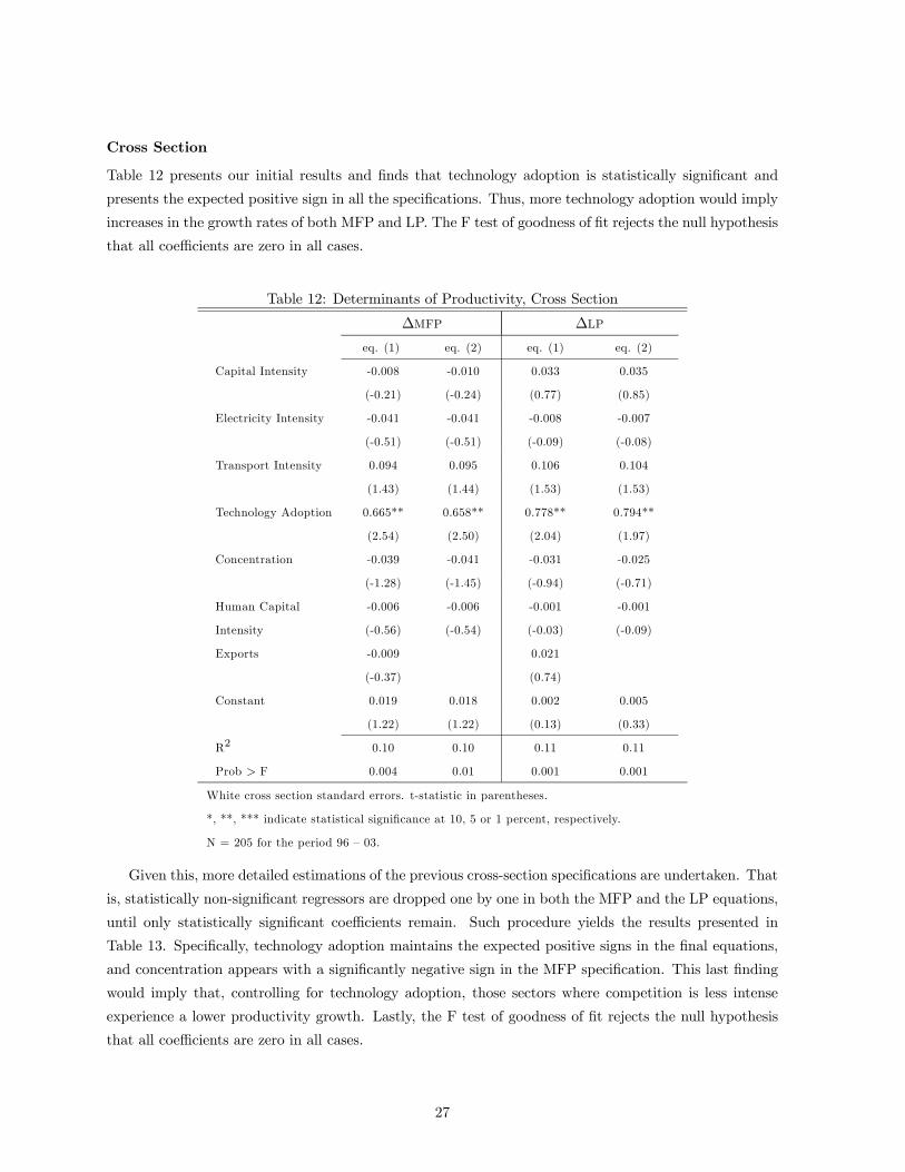
Cross Section
Table 12 presents our initial results and finds that technology adoption is statistically significant and
presents the expected positive sign in all the specifications. Thus, more technology adoption would imply
increases in the growth rates of both MFP and LP. The F test of goodness of fit rejects the null hypothesis
that all coefficients are zero in all cases.
Table 12: Determinants of Productivity, Cross Section
∆MFP ∆LP
eq. (1) eq. (2) eq. (1) eq. (2)
Capital Intensity -0.008 -0.010 0.033 0.035
(-0.21) (-0.24) (0.77) (0.85)
Electricity Intensity -0.041 -0.041 -0.008 -0.007
(-0.51) (-0.51) (-0.09) (-0.08)
Transport Intensity 0.094 0.095 0.106 0.104
(1.43) (1.44) (1.53) (1.53)
Technology Adoption 0.665** 0.658** 0.778** 0.794**
(2.54) (2.50) (2.04) (1.97)
Concentration -0.039 -0.041 -0.031 -0.025
(-1.28) (-1.45) (-0.94) (-0.71)
Human Capital -0.006 -0.006 -0.001 -0.001
Intensity (-0.56) (-0.54) (-0.03) (-0.09)
Exports -0.009 0.021
(-0.37) (0.74)
Constant 0.019 0.018 0.002 0.005
(1.22) (1.22) (0.13) (0.33)
R2 0.10 0.10 0.11 0.11
Prob > F 0.004 0.01 0.001 0.001
White cross section standard errors. t-statistic in parentheses.
*, **, *** indicate statistical significance at 10, 5 or 1 percent, respectively.
N = 205 for the period 96 — 03.
Given this, more detailed estimations of the previous cross-section specifications are undertaken. That
is, statistically non-significant regressors are dropped one by one in both the MFP and the LP equations,
until only statistically significant coefficients remain. Such procedure yields the results presented in
Table 13. Specifically, technology adoption maintains the expected positive signs in the final equations,
and concentration appears with a significantly negative sign in the MFP specification. This last finding
would imply that, controlling for technology adoption, those sectors where competition is less intense
experience a lower productivity growth. Lastly, the F test of goodness of fit rejects the null hypothesis
that all coefficients are zero in all cases.
27
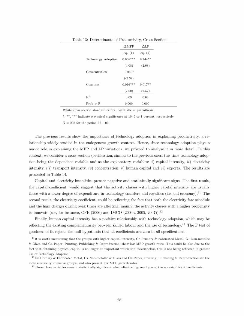
Table 13: Determinants of Productivity, Cross Section
∆MFP ∆LP
eq. (1) eq. (2)
Technology Adoption 0.668*** 0.744**
(4.08) (2.08)
Concentration -0.049*
(-2.37)
Constant 0.016*** 0.017**
(2.60) (2.52)
R2 0.09 0.09
Prob > F 0.000 0.000
White cross section standard errors. t-statistic in parenthesis.
*, **, *** indicate statistical significance at 10, 5 or 1 percent, respectively.
N = 205 for the period 96 — 03.
The previous results show the importance of technology adoption in explaining productivity, a re-
lationship widely studied in the endogenous growth context. Hence, since technology adoption plays a
major role in explaining the MFP and LP variations, we proceed to analyse it in more detail. In this
context, we consider a cross-section specification, similar to the previous ones, this time technology adop-
tion being the dependent variable and as the explanatory variables: i) capital intensity, ii) electricity
intensity, iii) transport intensity, iv) concentration, v) human capital and vi) exports. The results are
presented in Table 14.
Capital and electricity intensities present negative and statistically significant signs. The first result,
the capital coefficient, would suggest that the activity classes with higher capital intensity are usually
those with a lower degree of expenditure in technology transfers and royalties (i.e. old economy).41 The
second result, the electricity coefficient, could be reflecting the fact that both the electricity fare schedule
and the high charges during peak times are affecting, mainly, the activity classes with a higher propensity
to innovate (see, for instance, CFE (2006) and IMCO (2004a, 2005, 2007)).42
Finally, human capital intensity has a positive relationship with technology adoption, which may be
reflecting the existing complementarity between skilled labour and the use of technology.43 The F test of
goodness of fit rejects the null hypothesis that all coefficients are zero in all specifications.
41 It is worth mentioning that the groups with higher capital intensity, G8 Primary & Fabricated Metal, G7 Non-metallic
& Glass and G4 Paper, Printing, Publishing & Reproduction, show low MFP growth rates. This could be also due to the
fact that obtaining physical capital is no longer an important restriction; nevertheless, this is not being reflected in greater
use or technology adoption.42G8 Primary & Fabricated Metal, G7 Non-metallic & Glass and G4 Paper, Printing, Publishing & Reproduction are the
more electricity intensive groups, and also present low MFP growth rates.43These three variables remain statistically significant when eliminating, one by one, the non-significant coefficients.
28
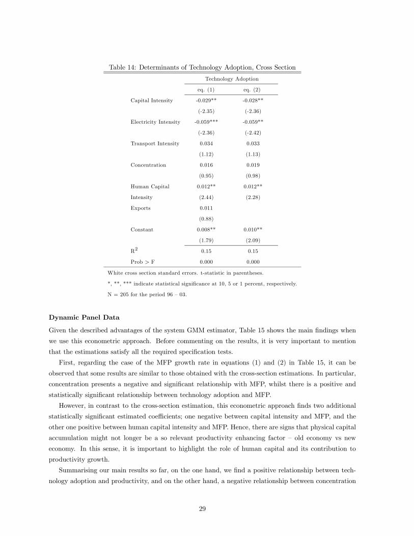
Table 14: Determinants of Technology Adoption, Cross Section
Technology Adoption
eq. (1) eq. (2)
Capital Intensity -0.029** -0.028**
(-2.35) (-2.36)
Electricity Intensity -0.059*** -0.059**
(-2.36) (-2.42)
Transport Intensity 0.034 0.033
(1.12) (1.13)
Concentration 0.016 0.019
(0.95) (0.98)
Human Capital 0.012** 0.012**
Intensity (2.44) (2.28)
Exports 0.011
(0.88)
Constant 0.008** 0.010**
(1.79) (2.09)
R2 0.15 0.15
Prob > F 0.000 0.000
White cross section standard errors. t-statistic in parentheses.
*, **, *** indicate statistical significance at 10, 5 or 1 percent, respectively.
N = 205 for the period 96 — 03.
Dynamic Panel Data
Given the described advantages of the system GMM estimator, Table 15 shows the main findings when
we use this econometric approach. Before commenting on the results, it is very important to mention
that the estimations satisfy all the required specification tests.
First, regarding the case of the MFP growth rate in equations (1) and (2) in Table 15, it can be
observed that some results are similar to those obtained with the cross-section estimations. In particular,
concentration presents a negative and significant relationship with MFP, whilst there is a positive and
statistically significant relationship between technology adoption and MFP.
However, in contrast to the cross-section estimation, this econometric approach finds two additional
statistically significant estimated coefficients; one negative between capital intensity and MFP, and the
other one positive between human capital intensity and MFP. Hence, there are signs that physical capital
accumulation might not longer be a so relevant productivity enhancing factor — old economy vs new
economy. In this sense, it is important to highlight the role of human capital and its contribution to
productivity growth.
Summarising our main results so far, on the one hand, we find a positive relationship between tech-
nology adoption and productivity, and on the other hand, a negative relationship between concentration
29
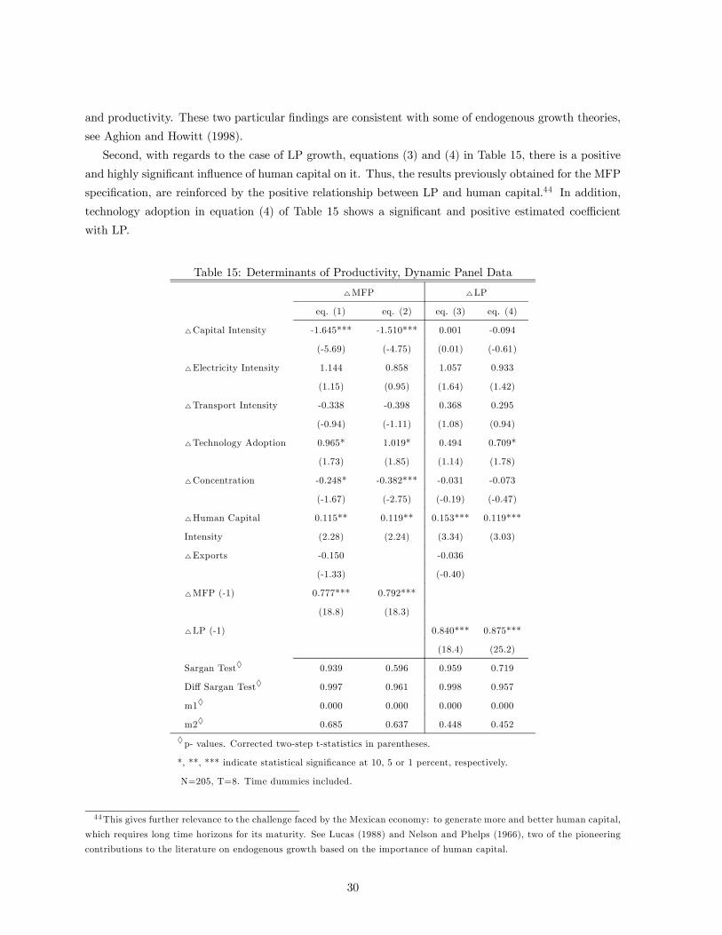
and productivity. These two particular findings are consistent with some of endogenous growth theories,
see Aghion and Howitt (1998).
Second, with regards to the case of LP growth, equations (3) and (4) in Table 15, there is a positive
and highly significant influence of human capital on it. Thus, the results previously obtained for the MFP
specification, are reinforced by the positive relationship between LP and human capital.44 In addition,
technology adoption in equation (4) of Table 15 shows a significant and positive estimated coefficient
with LP.
Table 15: Determinants of Productivity, Dynamic Panel Data
4MFP 4LP
eq. (1) eq. (2) eq. (3) eq. (4)
4Capital Intensity -1.645*** -1.510*** 0.001 -0.094
(-5.69) (-4.75) (0.01) (-0.61)
4Electricity Intensity 1.144 0.858 1.057 0.933
(1.15) (0.95) (1.64) (1.42)
4Transport Intensity -0.338 -0.398 0.368 0.295
(-0.94) (-1.11) (1.08) (0.94)
4Technology Adoption 0.965* 1.019* 0.494 0.709*
(1.73) (1.85) (1.14) (1.78)
4Concentration -0.248* -0.382*** -0.031 -0.073
(-1.67) (-2.75) (-0.19) (-0.47)
4Human Capital 0.115** 0.119** 0.153*** 0.119***
Intensity (2.28) (2.24) (3.34) (3.03)
4Exports -0.150 -0.036
(-1.33) (-0.40)
4MFP (-1) 0.777*** 0.792***
(18.8) (18.3)
4LP (-1) 0.840*** 0.875***
(18.4) (25.2)
Sargan Test♦ 0.939 0.596 0.959 0.719
Diff Sargan Test♦ 0.997 0.961 0.998 0.957
m1♦ 0.000 0.000 0.000 0.000
m2♦ 0.685 0.637 0.448 0.452
♦p- values. Corrected two-step t-statistics in parentheses.
*, **, *** indicate statistical significance at 10, 5 or 1 percent, respectively.
N=205, T=8. Time dummies included.
44This gives further relevance to the challenge faced by the Mexican economy: to generate more and better human capital,
which requires long time horizons for its maturity. See Lucas (1988) and Nelson and Phelps (1966), two of the pioneering
contributions to the literature on endogenous growth based on the importance of human capital.
30
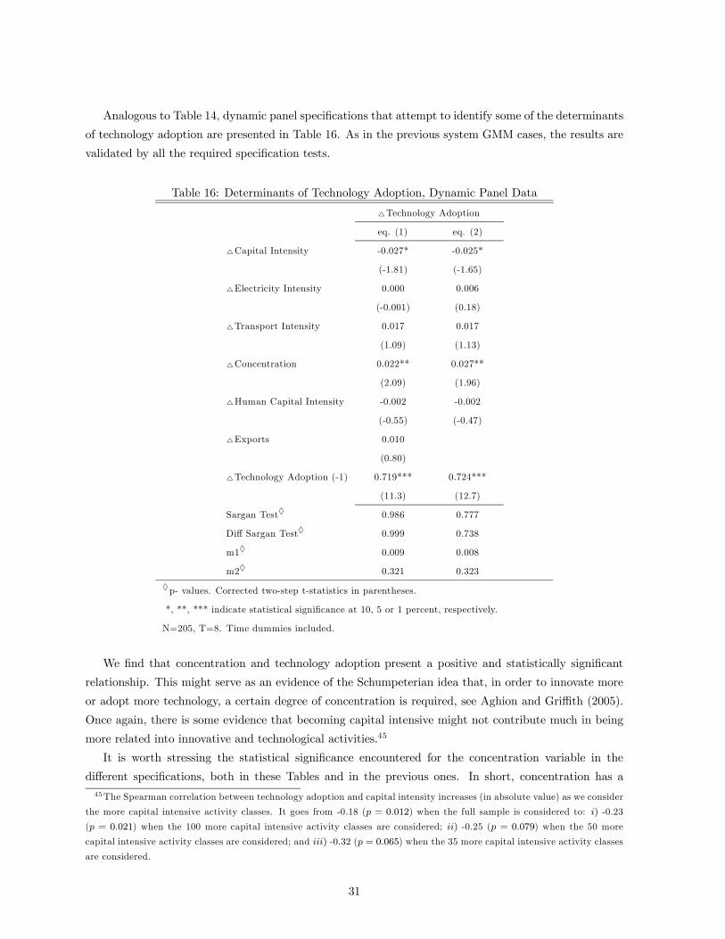
Analogous to Table 14, dynamic panel specifications that attempt to identify some of the determinants
of technology adoption are presented in Table 16. As in the previous system GMM cases, the results are
validated by all the required specification tests.
Table 16: Determinants of Technology Adoption, Dynamic Panel Data
4Technology Adoption
eq. (1) eq. (2)
4Capital Intensity -0.027* -0.025*
(-1.81) (-1.65)
4Electricity Intensity 0.000 0.006
(-0.001) (0.18)
4Transport Intensity 0.017 0.017
(1.09) (1.13)
4Concentration 0.022** 0.027**
(2.09) (1.96)
4Human Capital Intensity -0.002 -0.002
(-0.55) (-0.47)
4Exports 0.010
(0.80)
4Technology Adoption (-1) 0.719*** 0.724***
(11.3) (12.7)
Sargan Test♦ 0.986 0.777
Diff Sargan Test♦ 0.999 0.738
m1♦ 0.009 0.008
m2♦ 0.321 0.323
♦p- values. Corrected two-step t-statistics in parentheses.
*, **, *** indicate statistical significance at 10, 5 or 1 percent, respectively.
N=205, T=8. Time dummies included.
We find that concentration and technology adoption present a positive and statistically significant
relationship. This might serve as an evidence of the Schumpeterian idea that, in order to innovate more
or adopt more technology, a certain degree of concentration is required, see Aghion and Griffith (2005).
Once again, there is some evidence that becoming capital intensive might not contribute much in being
more related into innovative and technological activities.45
It is worth stressing the statistical significance encountered for the concentration variable in the
different specifications, both in these Tables and in the previous ones. In short, concentration has a45The Spearman correlation between technology adoption and capital intensity increases (in absolute value) as we consider
the more capital intensive activity classes. It goes from -0.18 (p = 0.012) when the full sample is considered to: i) -0.23
(p = 0.021) when the 100 more capital intensive activity classes are considered; ii) -0.25 (p = 0.079) when the 50 more
capital intensive activity classes are considered; and iii) -0.32 (p = 0.065) when the 35 more capital intensive activity classes
are considered.
31

positive relationship with technology adoption, but a negative one with MFP growth. Similar results are
encountered by Nickell (1996) for the UK manufacturing sector, and Okada (2005) for Japan.46
In short, concentration is exerting a positive and significant (at the 5%) influence on innovation (only
in the dynamic panel estimation). However, once these two variables are included into the econometric
estimation where MFP is the dependent variable, technology adoption is contributing positively, at the
10% level of significance, to MFP, whereas concentration is affecting negatively, at the 1% level of signif-
icance, to MFP. Based on the results of Table 15 and Table 16, the net effect of concentration on MFP
is negative.47
Hence, our results seem to indicate that those sectors where competition is less intense experience a
lower MFP growth.
6 Summary
Throughout the diverse dimensions that analysed the evolution of the 14 manufacturing groups, as well as
their trends in MFP and LP growth, it was encountered that, in general, on the one hand, G13 Computer
& Electronic Products, was one of the best performers; on the other hand, G2 Textile, Apparel, Fur
Leather & Footwear and G3 Lumber & Wood, were amongst the worst performers.
We found evidence that labour mobility between both the 14 groups and the 205 activity classes has
not been an important source for the overall LP growth as it only contributed with 5.3 percent and 2.3
percent to the observed growth at each aggregation level, respectively. Moreover, those groups in which
the real wage growth has been greater than the increase in labour productivity are, precisely, the less
productive.
Both the calculated and estimated elasticities found are consistent with those obtained in other studies
for developed countries, in particular the ones for capital; this is a good indicator that our measure of
capital has been constructed adequately.
The change in MFP has been the main driver in explaining the growth rates changes of both VA and
LP. In the case of aggregate output growth, MFP helps explaining between 58 percent and 69 percent;
whilst it accounts for 62 percent of aggregate LP growth.
There is evidence that electricity (transport) is contributing , negatively (positively), to the traditional
Solow-residual measure (MFP with K and L). However, the fact that transport appears to help in
explaining the Solow residual should not mask the overall evolution of this sector. What the results are
probably showing is that productivity gains are taking place via transport, which possibly indicate that,
for manufacturers, it has been relatively easier to overcome the difficulties posed by this sector, than
those prevalent in the electricity sector.
With respect to the identification of some of the determinants of both MFP and LP, the cross-section
analysis indicates: i) that technology adoption has a positive influence on the productivity measures,
whilst market concentration, which implies less competition, is negatively related to MFP growth; and ii)
when considering some of the factors explaining technology adoption, the cross-section analysis encounters
a positive sign for human capital intensity whilst negative signs for capital and electricity intensities.
46For some related findings, see Aghion and Griffith (2005).47 -0.23 for equations in (1) and -0.35 for equations in (2).
32
In the dynamic panel data analysis, first, it is found that in addition to the cross-sectional results, on
the one hand, there is a negative relation between capital intensity and MFP and a positive one between
human capital and MFP; on the other hand, there exists a positive relation between human capital
intensity and LP. Second, the dynamic panel estimation finds as determinants of technology adoption,
concentration with a positive sign and capital intensity with a negative one.
In sum, using AIS data from 1996 to 2003 at the activity class level, the evidence encountered here
seems to suggest that, even after controlling for technology adoption, those sectors characterised by higher
levels of concentration (less competition) would experience lower productivity rates.
References
[1] Aghion, P. and R. Griffith. (2005). Competition and Growth: Reconciling Theory and Evidence. MIT
Press.
[2] Aghion, P. and P. Howitt. (1998). Endogenous Growth Theory. MIT Press.
[3] Anderson, T.W. and C. Hsiao. (1981). “Estimation of Dynamic Models with Error Components.”
Journal of the American Statistical Association, 76: 598-606.
[4] Arellano, M. and S. Bond. (1991). “Some Tests of Specification for Panel Data: Monte Carlo Evidence
and an Application to Employment Equations.” Review of Economic Studies, 58: 277-297.
[5] Arellano, M. and O. Bover. (1995). “Another Look at the Instrumental Variables Estimation of
Error-Components Models.” Journal of Econometrics, 68: 29-51.
[6] Basu, S. and J. G. Fernald. (1995). “Are Apparent Productive Spillovers a Figment of Specification
Error?” Journal of Monetary Economics. 36: 165-188.
[7] Bergoeing, R., P. J. Kehoe, T. J. Kehoe and R. Soto. (2002). “Decades Lost and Found: Mexico and
Chile since 1980”. Federal Reserve Bank of Minneapolis Quarterly Review. Winter.
[8] Bernard, A. B. and J. B. Jensen. (1999). “Exporting and Productivity”. Working Paper # 7135.
NBER. May.
[9] Biorn, E., K.G. Lindquist and T. Skjerpen. (2002). “Heterogeneity in Returns to Scale: A Random
Coefficient Analysis with Unbalanced Panel Data”. Journal of Productivity Analysis, 18: 39-57.
[10] Blundell, R. and S. Bond. (1998). “Initial Conditions and Moment Restrictions in Dynamic Panel
Data Models.” Journal of Econometrics, 87:115-143.
[11] Blundell, R. and S. Bond. (2000). “GMM Estimation with Persistent Panel Data: An Application
to Production Functions.” Econometric Reviews, 19(3): 321-340.
[12] Bond, S., C. Nauges and F. Windmeijer. (2005). “Unit Root: Identification and Testing in Micro
Panels”. Institute for Fiscal Studies Working Paper CWP07/05
33
[13] Calderon-Madrid, A. and A. Voicu. (2004). “Multifactorial Productivity Growth and Job Turnover
in Mexican Manufacturing Plants in the 1990s”. Institute for the Study of Labour Working Paper
993. January.
[14] Calderon-Madrid, A. and A. Voicu. (2005). “Assessing Heterogeneity of Plant Responses to Trade
Liberalization: Productivity, Job Creation and Destruction and Survival of Manufacturing Plants in
NAFTA”. Mimeo. July.
[15] Cameron, G., J. Proudman and S. Redding. (1997). “Deconstructing Growth in UK Manufacturing”.
Working Paper. Bank of England.
[16] Casacuberta, C., G. Fachola and N. Gandelman. (2004). “The Impact of Trade Liberalization on
Employment, Capital and Productivity Dynamics: Evidence from the Uruguayan Manufacturing
Sector”. Inter-American Development Bank Working Paper R-479. February.
[17] CFE. (2006). Factores de ajuste a las tarifas de baja, media y alta tensión por variaciones en los
precios de combustibles y la inflación nacional. Subdirección de Programación. Mexico. Available on
http://aplicaciones.cfe.gob.mx/aplicaciones/ccfe/tarifas/factores/factores.asp
[18] Disney, R., J. Haskel and Y. Heden. (2003). “Restructuring an Productivity growth in UK Manu-
facturing.” The Economic Journal, 113:666-694.
[19] Dwyer, D. W. (1996). “Are Fixed Effects Fixed?”. Working Paper. Center for Economic Studies,
U.S. Bureau of the Census.
[20] Eslava, M., J. Haltiwanger, A. Kugler and M. Kugler. (2004). “The Effects of Structural Reforms
on Productivity and Profitability Enhancing Reallocation: Evidence from Colombia.” Journal of
Developments Economics, 75: 333-371.
[21] Faal, E. (2005). “GDP Growth, Potential Output, and Output Gaps in Mexico”. International
Monetary Fund Working Paper WP/05/93. May.
[22] Griffith, R. (1999). “Using the ARD Establishment Level Data at Foreign Ownership and Produc-
tivity in the United Kingdom.” The Economic Journal, 109: F416-F442.
[23] Griliches, Z. and J. A. Hausman. (1986). “Errors in Variables in Panel Data.” Journal of Economet-
rics, 31: 93-118.
[24] Harrison, A. and G. Hanson. (1999). “Who Gains From Trade Reform? Some Remaining Puzzles”
Journal of Development Economics Vol. 59: 125—154.
[25] Hsiao, C. (2003) Analysis of Panel Data. 2nd Edition. Cambridge University Press, Cambridge.
[26] IMCO. (2004a). Análisis de la Competitividad de México. Mexico.
[27] IMCO. (2004b). Elementos para Mejorar la Competitividad del Transporte de Carga en México.
Mexico.
[28] IMCO. (2005). Mercado de Factores Eficientes: Energía. Mexico.
34
[29] IMCO. (2007). “Competitividad de las Tarifas del Sector Eléctrico en México”. Presentation in Ciclo
de Conferencias con Legisladores. Mexico.
[30] International Energy Agency and Organisation for Economic Cooperation and Development. (2005).
Energy Prices and Taxes Quarterly Statistics. Volume 2005 Issue 4.
[31] Klette, T. J. (1999). “Market Power, Scale Economies and Productivity: Estimates from a Panel of
Establishment Data”. The Journal of Industrial Economics, Vol. 47(4): 451-476.
[32] Lopez-Cordova, E. (2002). “NAFTA and Mexico’s Manufacturing Productivity: An Empirical In-
vestigation using Micro-level Data.” Working Paper presented at the Latin American and Caribbean
Economic Association Meeting, Madrid.
[33] Lopez-Cordova, E. and M. Mesquita-Moreira. (2003). “Regional integration and Productivity: the
Experiences of Brazil and Mexico”. The Institute for the Integration of Latin America and the
Caribbean Working Paper 14. July.
[34] Lucas, R. E. (1988). “On the Mechanics of Economic Development.” Journal of Monetary Economics
22(1): 3-42.
[35] Mairesse, J. and B. H. Hall. (1996). “Estimating the Productivity of Research and Development:
An Exploration of GMM Methods using Data on French and United States Manufacturing Firms”.
Working Paper # 5501. NBER. March.
[36] Mena-Campos, D. (1997). “Acervos y Rendimiento del Capital en México, 1960-1997”. BSc. Thesis
in Economics. ITAM. July.
[37] Nelson, C. and E. Phelps. (1966). “Investment in Humans, Technological Diffusion, and Economic
Growth.” American Economic Review 61: 69-75.
[38] Nickell, S. J. (1981). “Biases in Dynamic Model with Fixed Effects” Econometrica 49: 1417-1426.
[39] Nickell, S. J. (1996). “Competition and Corporate Performance.” Journal of Political Economy, Vol.
104(4): 724-746.
[40] OECD. (2001). “Measurement of Aggregate and Industry-Level Productivity Growth”. OECD Man-
ual. Paris.
[41] Okada, Y. (2005). “Competition and Productivity in Japanese Manufacturing Industries”. Working
Paper # 11540. NBER. August.
[42] Pavcnik, N. (2002). “Trade Liberalization, Exit, and Productivity Improvements: Evidence from
Chilean Plants.” Review of Economic Studies, 69: 245-276.
[43] Perez-Gonzalez, F. (2004). “The Impact of Acquiring Control on Productivity: Evidence from Mex-
ican Manufacturing Plants.” Mimeo, Columbia University.
[44] World Bank. (2006). “Mexico’s Competitiveness: Reaching Its Potential.” World Bank Report No.
35388-MX. Washington, D.C. August.
35

[45] World Economic Forum. (2006). The Global Competitiveness Report 2006-2007.
[46] Young, A. (1995). “The Tyranny of Numbers: Confronting the Statistical Realities of the East Asian
Growth Experience.” Quarterly Journal of Economics 110: 641-680.
Appendix
Groups Composition
Each manufacturing group is composed mainly by the following activities and products:
G1. Food, Beverage & Tobacco: Meat processing, dairy, cereals, bakery, tortilla, sugar industry,
sweets, coffee, alcohol, beverages, tobacco.
G2. Textile, Apparel, Fur, Leather & Footwear: Fibers, fabrics, clothes, leather goods, fur, shoes.
G3. Lumber & Wood: Wood processing, construction supplies and containers.
G4. Paper, Printing, Publishing & Reproduction: Manufacturing of paper products, prints, newspa-
pers, books, magazines.
G5. Petroleum & Coal: Coke, mineral oils and additives.
G6. Chemicals: Basic oil chemistry, fertilizers, insecticides, resins, paints, pharmaceutical, perfumes,
tires, rubber, tubing, plastic house supplies.
G7. Non-metallic & Glass: Construction materials, glass, cement, concrete, ceramic.
G8. Primary & Fabricated Metal: Iron, steel, alloys, aluminium, heaters.
G9. Machinery: Tractors, machinery, agricultural supplies, pumps, filters.
G10. Electrical Equipment, Appliances & Components: stoves, ovens, refrigerators, washing machines,
heaters, boilers, batteries, bulbs, automotive electric components.
G11. Automobiles: Production, assembly and repair of automobiles, trucks, engines, motors, trans-
missions, suspensions, brakes.
G12. Other Transportation Equipment: Production, assembly and repair of navigation ships and
boats, railroad equipment, motorcycles, bicycles and parts.
G13. Computer & Electronic Products: Computers, radios, TV sets, photography, medical equipment,
measurement equipment, lenses.
G14. Miscellaneous: Jewelry, toys, office supplies, mattresses, furniture.
36
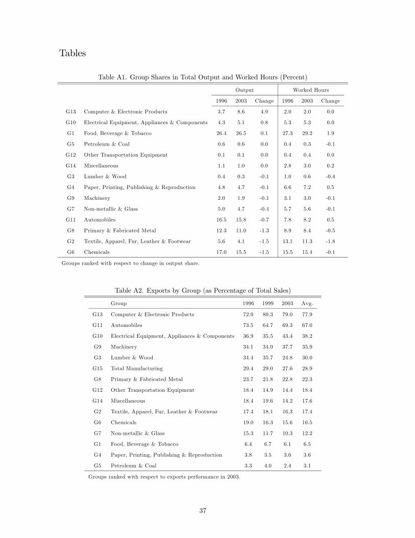
Tables
Table A1. Group Shares in Total Output and Worked Hours (Percent)
Output Worked Hours
1996 2003 Change 1996 2003 Change
G13 Computer & Electronic Products 3.7 8.6 4.9 2.0 2.0 0.0
G10 Electrical Equipment, Appliances & Components 4.3 5.1 0.8 5.3 5.3 0.0
G1 Food, Beverage & Tobacco 26.4 26.5 0.1 27.3 29.2 1.9
G5 Petroleum & Coal 0.6 0.6 0.0 0.4 0.3 -0.1
G12 Other Transportation Equipment 0.1 0.1 0.0 0.4 0.4 0.0
G14 Miscellaneous 1.1 1.0 0.0 2.8 3.0 0.2
G3 Lumber & Wood 0.4 0.3 -0.1 1.0 0.6 -0.4
G4 Paper, Printing, Publishing & Reproduction 4.8 4.7 -0.1 6.6 7.2 0.5
G9 Machinery 2.0 1.9 -0.1 3.1 3.0 -0.1
G7 Non-metallic & Glass 5.0 4.7 -0.4 5.7 5.6 -0.1
G11 Automobiles 16.5 15.8 -0.7 7.8 8.2 0.5
G8 Primary & Fabricated Metal 12.3 11.0 -1.3 8.9 8.4 -0.5
G2 Textile, Apparel, Fur, Leather & Footwear 5.6 4.1 -1.5 13.1 11.3 -1.8
G6 Chemicals 17.0 15.5 -1.5 15.5 15.4 -0.1
Groups ranked with respect to change in output share.
Table A2. Exports by Group (as Percentage of Total Sales)
Group 1996 1999 2003 Avg.
G13 Computer & Electronic Products 72.9 80.3 79.0 77.9
G11 Automobiles 73.5 64.7 69.3 67.0
G10 Electrical Equipment, Appliances & Components 36.9 35.5 43.4 38.2
G9 Machinery 34.1 34.0 37.7 35.9
G3 Lumber & Wood 34.4 35.7 24.8 30.0
G15 Total Manufacturing 29.4 29.0 27.6 28.9
G8 Primary & Fabricated Metal 23.7 21.8 22.8 22.3
G12 Other Transportation Equipment 18.4 14.9 14.4 18.4
G14 Miscellaneous 18.4 19.6 14.2 17.6
G2 Textile, Apparel, Fur, Leather & Footwear 17.4 18.1 16.3 17.4
G6 Chemicals 19.0 16.3 15.6 16.5
G7 Non-metallic & Glass 15.3 11.7 10.3 12.2
G1 Food, Beverage & Tobacco 6.4 6.7 6.1 6.5
G4 Paper, Printing, Publishing & Reproduction 3.8 3.5 3.6 3.6
G5 Petroleum & Coal 3.3 4.0 2.4 3.1
Groups ranked with respect to exports performance in 2003.
37
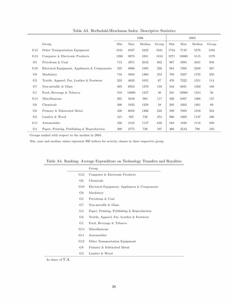
Table A3. Herfindahl-Hirschman Index: Descriptive Statistics
1996 2003
Group Min Max Median Group Min Max Median Group
G12 Other Transportation Equipment 1841 6107 3422 1041 1744 7145 5578 1234
G13 Computer & Electronic Products 1390 9973 4281 1810 2271 10000 5115 1579
G5 Petroleum & Coal 713 4971 2842 802 967 5994 3481 948
G10 Electrical Equipment, Appliances & Components 535 8866 1895 226 884 7395 2288 267
G9 Machinery 716 5683 1360 253 703 5207 1735 250
G2 Textile, Apparel, Fur, Leather & Footwear 233 4620 1055 67 476 7222 1551 114
G7 Non-metallic & Glass 305 6952 1270 158 344 6031 1502 160
G1 Food, Beverage & Tobacco 210 10000 1227 40 231 10000 1454 50
G14 Miscellaneous 265 3849 994 117 330 6407 1368 157
G6 Chemicals 200 5832 1229 58 295 4203 1261 69
G8 Primary & Fabricated Metal 426 6058 1306 228 599 7805 1216 224
G3 Lumber & Wood 415 925 756 374 960 1669 1137 486
G11 Automobiles 456 2125 1147 646 583 1838 1118 839
G4 Paper, Printing, Publishing & Reproduction 309 2775 726 107 366 2543 798 103
Groups ranked with respect to the median in 2003.
Min, max and median values represent HH indices for activity classes in their respective group.
Table A4. Ranking: Average Expenditure on Technology Transfers and Royalties
Group
G13 Computer & Electronic Products
G6 Chemicals
G10 Electrical Equipment, Appliances & Components
G9 Machinery
G5 Petroleum & Coal
G7 Non-metallic & Glass
G4 Paper, Printing, Publishing & Reproduction
G2 Textile, Apparel, Fur, Leather & Footwear
G1 Food, Beverage & Tobacco
G14 Miscellaneous
G11 Automobiles
G12 Other Transportation Equipment
G8 Primary & Fabricated Metal
G3 Lumber & Wood
As share of V A.
38
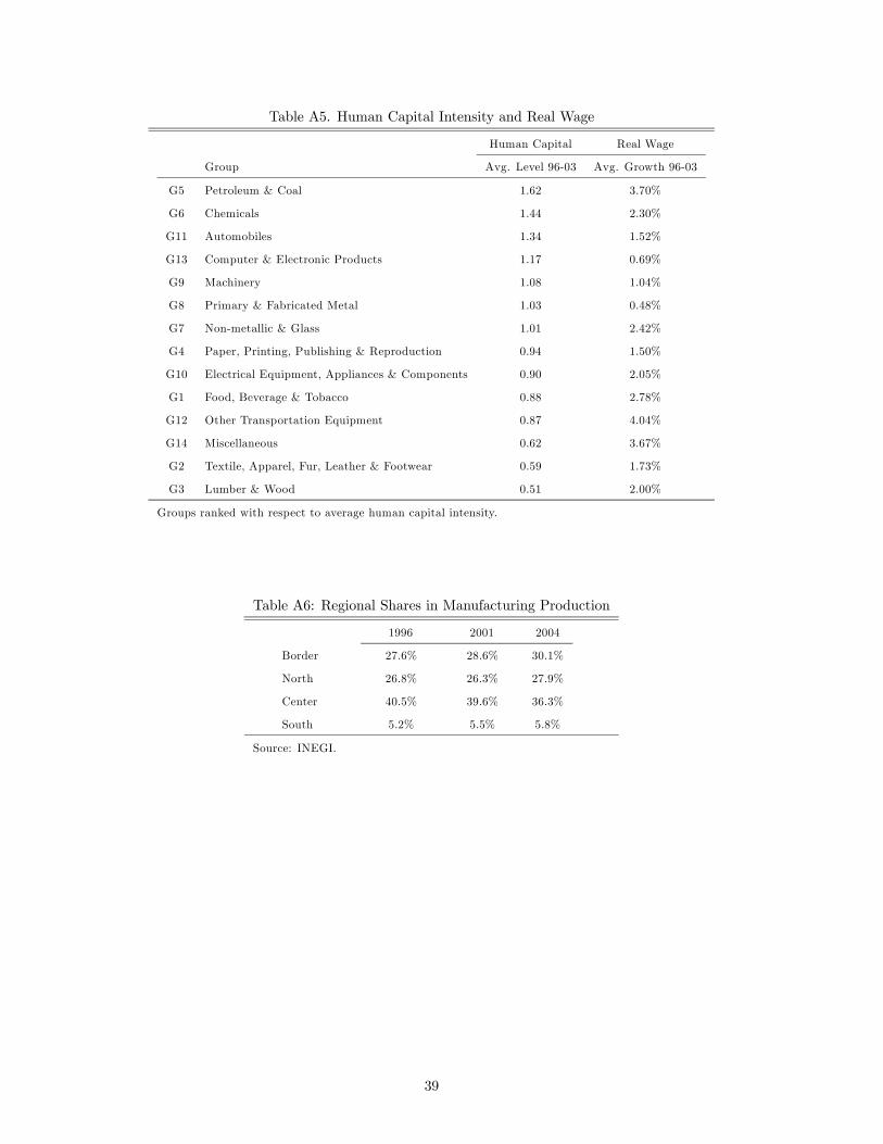
Table A5. Human Capital Intensity and Real Wage
Human Capital Real Wage
Group Avg. Level 96-03 Avg. Growth 96-03
G5 Petroleum & Coal 1.62 3.70%
G6 Chemicals 1.44 2.30%
G11 Automobiles 1.34 1.52%
G13 Computer & Electronic Products 1.17 0.69%
G9 Machinery 1.08 1.04%
G8 Primary & Fabricated Metal 1.03 0.48%
G7 Non-metallic & Glass 1.01 2.42%
G4 Paper, Printing, Publishing & Reproduction 0.94 1.50%
G10 Electrical Equipment, Appliances & Components 0.90 2.05%
G1 Food, Beverage & Tobacco 0.88 2.78%
G12 Other Transportation Equipment 0.87 4.04%
G14 Miscellaneous 0.62 3.67%
G2 Textile, Apparel, Fur, Leather & Footwear 0.59 1.73%
G3 Lumber & Wood 0.51 2.00%
Groups ranked with respect to average human capital intensity.
Table A6: Regional Shares in Manufacturing Production
1996 2001 2004
Border 27.6% 28.6% 30.1%
North 26.8% 26.3% 27.9%
Center 40.5% 39.6% 36.3%
South 5.2% 5.5% 5.8%
Source: INEGI.
39
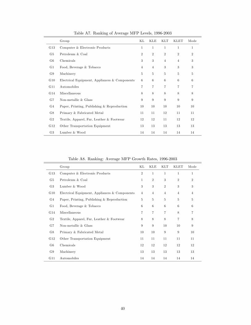
Table A7. Ranking of Average MFP Levels, 1996-2003
Group KL KLE KLT KLET Mode
G13 Computer & Electronic Products 1 1 1 1 1
G5 Petroleum & Coal 2 2 2 2 2
G6 Chemicals 3 3 4 4 3
G1 Food, Beverage & Tobacco 4 4 3 3 3
G9 Machinery 5 5 5 5 5
G10 Electrical Equipment, Appliances & Components 6 6 6 6 6
G11 Automobiles 7 7 7 7 7
G14 Miscellaneous 8 8 8 8 8
G7 Non-metallic & Glass 9 9 9 9 9
G4 Paper, Printing, Publishing & Reproduction 10 10 10 10 10
G8 Primary & Fabricated Metal 11 11 12 11 11
G2 Textile, Apparel, Fur, Leather & Footwear 12 12 11 12 12
G12 Other Transportation Equipment 13 13 13 13 13
G3 Lumber & Wood 14 14 14 14 14
Table A8. Ranking: Average MFP Growth Rates, 1996-2003
Group KL KLE KLT KLET Mode
G13 Computer & Electronic Products 2 1 1 1 1
G5 Petroleum & Coal 1 2 3 2 2
G3 Lumber & Wood 3 3 2 3 3
G10 Electrical Equipment, Appliances & Components 4 4 4 4 4
G4 Paper, Printing, Publishing & Reproduction 5 5 5 5 5
G1 Food, Beverage & Tobacco 6 6 6 6 6
G14 Miscellaneous 7 7 7 8 7
G2 Textile, Apparel, Fur, Leather & Footwear 8 8 8 7 8
G7 Non-metallic & Glass 9 9 10 10 9
G8 Primary & Fabricated Metal 10 10 9 9 10
G12 Other Transportation Equipment 11 11 11 11 11
G6 Chemicals 12 12 12 12 12
G9 Machinery 13 13 13 13 13
G11 Automobiles 14 14 14 14 14
40
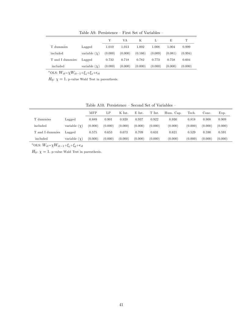
Table A9. Persistence — First Set of Variables —
Y VA K L E T
T dummies Lagged 1.010 1.013 1.002 1.008 1.004 0.999
included variable (χ) (0.000) (0.000) (0.166) (0.009) (0.081) (0.994)
T and I dummies Lagged 0.732 0.718 0.782 0.773 0.758 0.604
included variable (χ) (0.000) (0.000) (0.000) (0.000) (0.000) (0.000)
◦OLS: Wit=χWit−1+ξi+ξt+ it
H0: χ = 1. p-value Wald Test in parenthesis.
Table A10. Persistence — Second Set of Variables —
MFP LP K Int. E Int. T Int. Hum. Cap. Tech. Conc. Exp.
T dummies Lagged 0.889 0.901 0.920 0.937 0.922 0.930 0.818 0.908 0.909
included variable (χ) (0.000) (0.000) (0.000) (0.000) (0.000) (0.000) (0.000) (0.000) (0.000)
T and I dummies Lagged 0.575 0.653 0.673 0.709 0.631 0.621 0.529 0.590 0.591
included variable (χ) (0.000) (0.000) (0.000) (0.000) (0.000) (0.000) (0.000) (0.000) (0.000)
◦OLS: Wit=χWit−1+ξi+ξt+ it
H0: χ = 1. p-value Wald Test in parenthesis.
41
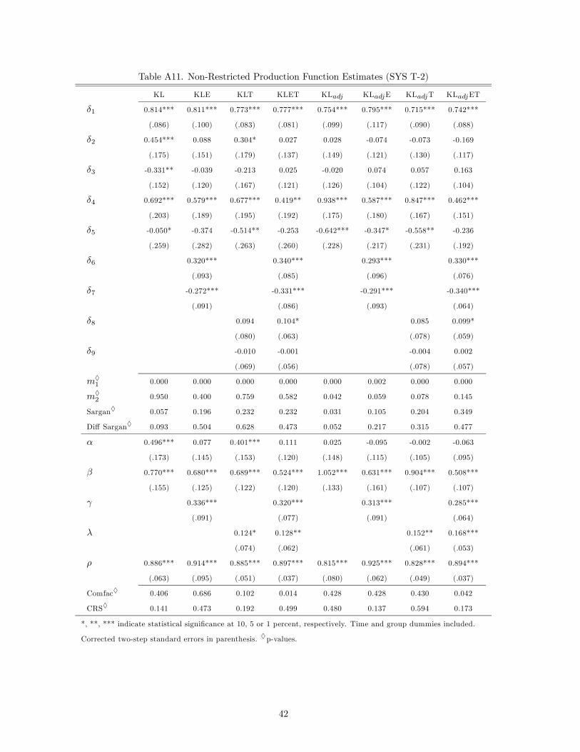
Table A11. Non-Restricted Production Function Estimates (SYS T-2)
KL KLE KLT KLET KLadj KLadjE KLadjT KLadjET
δ1 0.814*** 0.811*** 0.773*** 0.777*** 0.754*** 0.795*** 0.715*** 0.742***
(.086) (.100) (.083) (.081) (.099) (.117) (.090) (.088)
δ2 0.454*** 0.088 0.304* 0.027 0.028 -0.074 -0.073 -0.169
(.175) (.151) (.179) (.137) (.149) (.121) (.130) (.117)
δ3 -0.331** -0.039 -0.213 0.025 -0.020 0.074 0.057 0.163
(.152) (.120) (.167) (.121) (.126) (.104) (.122) (.104)
δ4 0.692*** 0.579*** 0.677*** 0.419** 0.938*** 0.587*** 0.847*** 0.462***
(.203) (.189) (.195) (.192) (.175) (.180) (.167) (.151)
δ5 -0.050* -0.374 -0.514** -0.253 -0.642*** -0.347* -0.558** -0.236
(.259) (.282) (.263) (.260) (.228) (.217) (.231) (.192)
δ6 0.320*** 0.340*** 0.293*** 0.330***
(.093) (.085) (.096) (.076)
δ7 -0.272*** -0.331*** -0.291*** -0.340***
(.091) (.086) (.093) (.064)
δ8 0.094 0.104* 0.085 0.099*
(.080) (.063) (.078) (.059)
δ9 -0.010 -0.001 -0.004 0.002
(.069) (.056) (.078) (.057)
m♦1 0.000 0.000 0.000 0.000 0.000 0.002 0.000 0.000
m♦2 0.950 0.400 0.759 0.582 0.042 0.059 0.078 0.145
Sargan♦ 0.057 0.196 0.232 0.232 0.031 0.105 0.204 0.349
Diff Sargan♦ 0.093 0.504 0.628 0.473 0.052 0.217 0.315 0.477
α 0.496*** 0.077 0.401*** 0.111 0.025 -0.095 -0.002 -0.063
(.173) (.145) (.153) (.120) (.148) (.115) (.105) (.095)
β 0.770*** 0.680*** 0.689*** 0.524*** 1.052*** 0.631*** 0.904*** 0.508***
(.155) (.125) (.122) (.120) (.133) (.161) (.107) (.107)
γ 0.336*** 0.320*** 0.313*** 0.285***
(.091) (.077) (.091) (.064)
λ 0.124* 0.128** 0.152** 0.168***
(.074) (.062) (.061) (.053)
ρ 0.886*** 0.914*** 0.885*** 0.897*** 0.815*** 0.925*** 0.828*** 0.894***
(.063) (.095) (.051) (.037) (.080) (.062) (.049) (.037)
Comfac♦ 0.406 0.686 0.102 0.014 0.428 0.428 0.430 0.042
CRS♦ 0.141 0.473 0.192 0.499 0.480 0.137 0.594 0.173
*, **, *** indicate statistical significance at 10, 5 or 1 percent, respectively. Time and group dummies included.
Corrected two-step standard errors in parenthesis. ♦p-values.
42
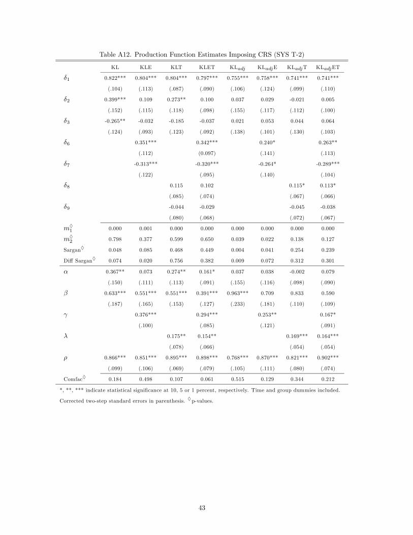
Table A12. Production Function Estimates Imposing CRS (SYS T-2)
KL KLE KLT KLET KLadj KLadjE KLadjT KLadjET
δ1 0.822*** 0.804*** 0.804*** 0.797*** 0.755*** 0.758*** 0.741*** 0.741***
(.104) (.113) (.087) (.090) (.106) (.124) (.099) (.110)
δ2 0.399*** 0.109 0.273** 0.100 0.037 0.029 -0.021 0.005
(.152) (.115) (.118) (.098) (.155) (.117) (.112) (.100)
δ3 -0.265** -0.032 -0.185 -0.037 0.021 0.053 0.044 0.064
(.124) (.093) (.123) (.092) (.138) (.101) (.130) (.103)
δ6 0.351*** 0.342*** 0.240* 0.263**
(.112) (0.097) (.141) (.113)
δ7 -0.313*** -0.320*** -0.264* -0.289***
(.122) (.095) (.140) (.104)
δ8 0.115 0.102 0.115* 0.113*
(.085) (.074) (.067) (.066)
δ9 -0.044 -0.029 -0.045 -0.038
(.080) (.068) (.072) (.067)
m♦1 0.000 0.001 0.000 0.000 0.000 0.000 0.000 0.000
m♦2 0.798 0.377 0.599 0.650 0.039 0.022 0.138 0.127
Sargan♦ 0.048 0.085 0.468 0.449 0.004 0.041 0.254 0.239
Diff Sargan♦ 0.074 0.020 0.756 0.382 0.009 0.072 0.312 0.301
α 0.367** 0.073 0.274** 0.161* 0.037 0.038 -0.002 0.079
(.150) (.111) (.113) (.091) (.155) (.116) (.098) (.090)
β 0.633*** 0.551*** 0.551*** 0.391*** 0.963*** 0.709 0.833 0.590
(.187) (.165) (.153) (.127) (.233) (.181) (.110) (.109)
γ 0.376*** 0.294*** 0.253** 0.167*
(.100) (.085) (.121) (.091)
λ 0.175** 0.154** 0.169*** 0.164***
(.078) (.066) (.054) (.054)
ρ 0.866*** 0.851*** 0.895*** 0.898*** 0.768*** 0.870*** 0.821*** 0.902***
(.099) (.106) (.069) (.079) (.105) (.111) (.080) (.074)
Comfac♦ 0.184 0.498 0.107 0.061 0.515 0.129 0.344 0.212
*, **, *** indicate statistical significance at 10, 5 or 1 percent, respectively. Time and group dummies included.
Corrected two-step standard errors in parenthesis. ♦p-values.
43
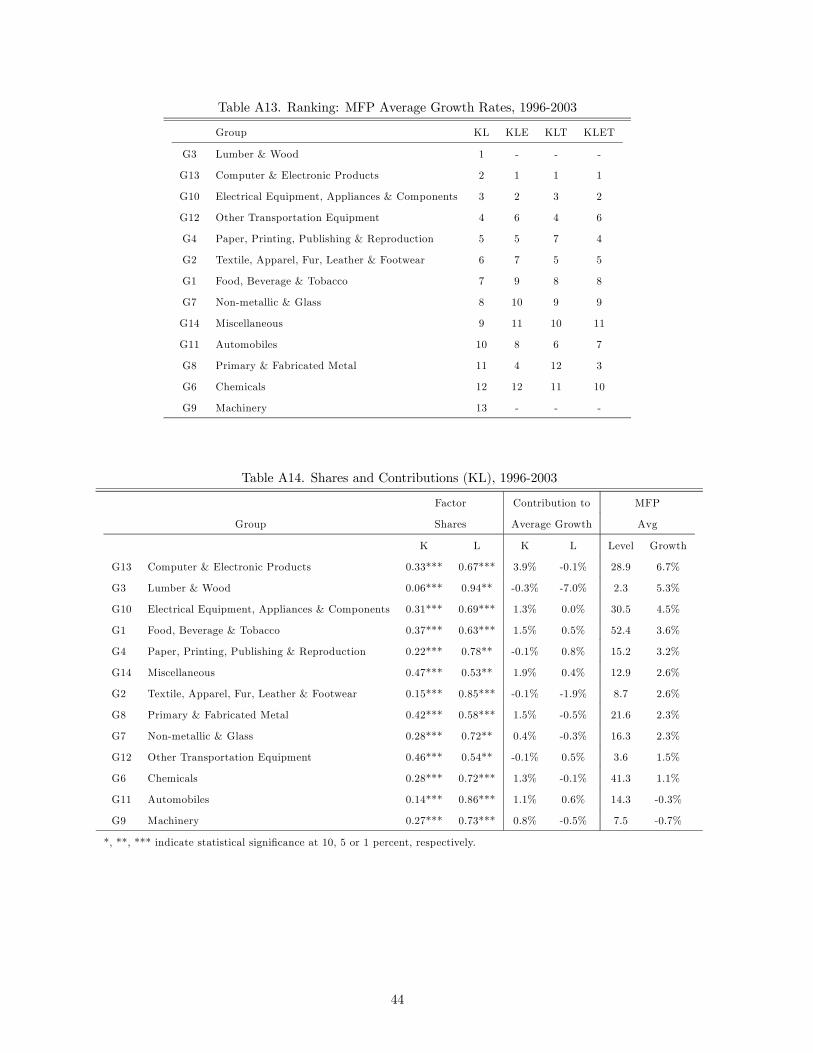
Table A13. Ranking: MFP Average Growth Rates, 1996-2003
Group KL KLE KLT KLET
G3 Lumber & Wood 1 - - -
G13 Computer & Electronic Products 2 1 1 1
G10 Electrical Equipment, Appliances & Components 3 2 3 2
G12 Other Transportation Equipment 4 6 4 6
G4 Paper, Printing, Publishing & Reproduction 5 5 7 4
G2 Textile, Apparel, Fur, Leather & Footwear 6 7 5 5
G1 Food, Beverage & Tobacco 7 9 8 8
G7 Non-metallic & Glass 8 10 9 9
G14 Miscellaneous 9 11 10 11
G11 Automobiles 10 8 6 7
G8 Primary & Fabricated Metal 11 4 12 3
G6 Chemicals 12 12 11 10
G9 Machinery 13 - - -
Table A14. Shares and Contributions (KL), 1996-2003
Factor Contribution to MFP
Group Shares Average Growth Avg
K L K L Level Growth
G13 Computer & Electronic Products 0.33*** 0.67*** 3.9% -0.1% 28.9 6.7%
G3 Lumber & Wood 0.06*** 0.94** -0.3% -7.0% 2.3 5.3%
G10 Electrical Equipment, Appliances & Components 0.31*** 0.69*** 1.3% 0.0% 30.5 4.5%
G1 Food, Beverage & Tobacco 0.37*** 0.63*** 1.5% 0.5% 52.4 3.6%
G4 Paper, Printing, Publishing & Reproduction 0.22*** 0.78** -0.1% 0.8% 15.2 3.2%
G14 Miscellaneous 0.47*** 0.53** 1.9% 0.4% 12.9 2.6%
G2 Textile, Apparel, Fur, Leather & Footwear 0.15*** 0.85*** -0.1% -1.9% 8.7 2.6%
G8 Primary & Fabricated Metal 0.42*** 0.58*** 1.5% -0.5% 21.6 2.3%
G7 Non-metallic & Glass 0.28*** 0.72** 0.4% -0.3% 16.3 2.3%
G12 Other Transportation Equipment 0.46*** 0.54** -0.1% 0.5% 3.6 1.5%
G6 Chemicals 0.28*** 0.72*** 1.3% -0.1% 41.3 1.1%
G11 Automobiles 0.14*** 0.86*** 1.1% 0.6% 14.3 -0.3%
G9 Machinery 0.27*** 0.73*** 0.8% -0.5% 7.5 -0.7%
*, **, *** indicate statistical significance at 10, 5 or 1 percent, respectively.
44
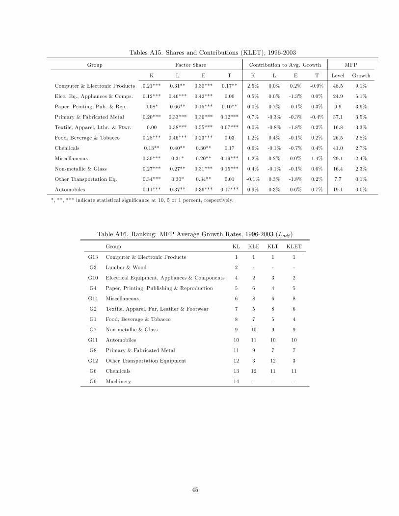
Tables A15. Shares and Contributions (KLET), 1996-2003
Group Factor Share Contribution to Avg. Growth MFP
K L E T K L E T Level Growth
Computer & Electronic Products 0.21*** 0.31** 0.30*** 0.17** 2.5% 0.0% 0.2% -0.9% 48.5 9.1%
Elec. Eq., Appliances & Comps. 0.12*** 0.46*** 0.42*** 0.00 0.5% 0.0% -1.3% 0.0% 24.9 5.1%
Paper, Printing, Pub. & Rep. 0.08* 0.66** 0.15*** 0.10** 0.0% 0.7% -0.1% 0.3% 9.9 3.9%
Primary & Fabricated Metal 0.20*** 0.33*** 0.36*** 0.12*** 0.7% -0.3% -0.3% -0.4% 37.1 3.5%
Textile, Apparel, Lthr. & Ftwr. 0.00 0.38*** 0.55*** 0.07*** 0.0% -0.8% -1.8% 0.2% 16.8 3.3%
Food, Beverage & Tobacco 0.28*** 0.46*** 0.23*** 0.03 1.2% 0.4% -0.1% 0.2% 26.5 2.8%
Chemicals 0.13** 0.40** 0.30** 0.17 0.6% -0.1% -0.7% 0.4% 41.0 2.7%
Miscellaneous 0.30*** 0.31* 0.20** 0.19*** 1.2% 0.2% 0.0% 1.4% 29.1 2.4%
Non-metallic & Glass 0.27*** 0.27** 0.31*** 0.15*** 0.4% -0.1% -0.1% 0.6% 16.4 2.3%
Other Transportation Eq. 0.34*** 0.30* 0.34** 0.01 -0.1% 0.3% -1.8% 0.2% 7.7 0.1%
Automobiles 0.11*** 0.37** 0.36*** 0.17*** 0.9% 0.3% 0.6% 0.7% 19.1 0.0%
*, **, *** indicate statistical significance at 10, 5 or 1 percent, respectively.
Table A16. Ranking: MFP Average Growth Rates, 1996-2003 (Ladj )
Group KL KLE KLT KLET
G13 Computer & Electronic Products 1 1 1 1
G3 Lumber & Wood 2 - - -
G10 Electrical Equipment, Appliances & Components 4 2 3 2
G4 Paper, Printing, Publishing & Reproduction 5 6 4 5
G14 Miscellaneous 6 8 6 8
G2 Textile, Apparel, Fur, Leather & Footwear 7 5 8 6
G1 Food, Beverage & Tobacco 8 7 5 4
G7 Non-metallic & Glass 9 10 9 9
G11 Automobiles 10 11 10 10
G8 Primary & Fabricated Metal 11 9 7 7
G12 Other Transportation Equipment 12 3 12 3
G6 Chemicals 13 12 11 11
G9 Machinery 14 - - -
45
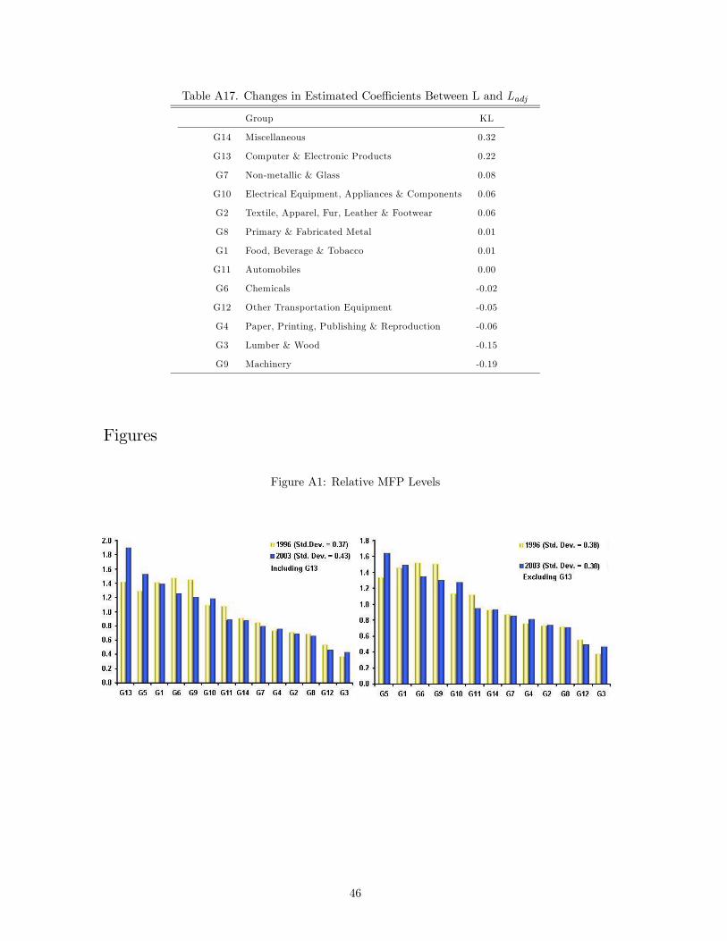
Table A17. Changes in Estimated Coefficients Between L and Ladj
Group KL
G14 Miscellaneous 0.32
G13 Computer & Electronic Products 0.22
G7 Non-metallic & Glass 0.08
G10 Electrical Equipment, Appliances & Components 0.06
G2 Textile, Apparel, Fur, Leather & Footwear 0.06
G8 Primary & Fabricated Metal 0.01
G1 Food, Beverage & Tobacco 0.01
G11 Automobiles 0.00
G6 Chemicals -0.02
G12 Other Transportation Equipment -0.05
G4 Paper, Printing, Publishing & Reproduction -0.06
G3 Lumber & Wood -0.15
G9 Machinery -0.19
Figures
Figure A1: Relative MFP Levels
46
Related Documents