Multidirectional wave transformation around detached breakwaters

(2007) 775–789www.elsevier.com/locate/coastaleng

Coastal Engineering 54

Multidirectional wave transformation around detached breakwaters

S. Ilic a,⁎, A.J. van der Westhuysen b, J.A. Roelvink c, A.J. Chadwick d

a Geography Department, Lancaster University, LA1 4YQ, UKb WL | Delft Hydraulics, P.O. Box 177, 2600 MH Delft, The Netherlands

c UNESCO-IHE Institute for Water Education, P.O. Box 3015, 2601 DA Delft, The Netherlandsd School of Engineering, University of Plymouth, Reynolds Building, Drake Circus, Plymouth PL4 8AA, UK

Received 10 September 2006; received in revised form 11 May 2007Available online 28 June 2007

Abstract

The performance of the new wave diffraction feature of the shallow-water spectral model SWAN, particularly its ability to predict themultidirectional wave transformation around shore-parallel emerged breakwaters is examined using laboratory and field data. Comparisonbetween model predictions and field measurements of directional spectra was used to identify the importance of various wave transformationprocesses in the evolution of the directional wave field. First, the model was evaluated against laboratory measurements of diffractedmultidirectional waves around a breakwater shoulder. Excellent agreement between the model predictions and measurements was found for broadfrequency and directional spectra. The performance of the model worsened with decreasing frequency and directional spread. Next, theperformance of the model with regard to diffraction–refraction was assessed for directional wave spectra around detached breakwaters. Sevendifferent field cases were considered: three wind–sea spectra with broad frequency and directional distributions, each coming from a differentdirection; two swell–sea bimodal spectra; and two swell spectra with narrow frequency and directional distributions. The new diffractionfunctionality in SWAN improved the prediction of wave heights around shore-parallel breakwaters. Processes such as beach reflection and wavetransmission through breakwaters seem to have a significant role on transformation of swell waves behind the breakwaters. Bottom friction andwave–current interactions were less important, while the difference in frequency and directional distribution might be associated with seiching.© 2007 Elsevier B.V. All rights reserved.

Keywords: Wave refraction–diffraction; Multidirectional waves; SWAN; Detached breakwaters; Wave transmission; Beach reflection

1. Introduction

The advantage of detached breakwaters compared to moretraditional shoreline structures is that they decrease the height ofincoming waves and reduce offshore sediment losses. As theyare mostly built in intermediate to shallow waters, the physicalprocesses that may be involved in wave transformation arounddetached breakwaters include: shoaling; refraction; diffraction;energy dissipation due to sea bed friction and wave breaking;interaction of waves and currents; wave reflections fromstructures and beaches; wave transmission through and over

⁎ Corresponding author. Tel.: +44 1524510264.E-mail addresses: [email protected] (S. Ilic),

[email protected] (A.J. van der Westhuysen),[email protected] (J.A. Roelvink), [email protected](A.J. Chadwick).

0378-3839/$ - see front matter © 2007 Elsevier B.V. All rights reserved.doi:10.1016/j.coastaleng.2007.05.002

permeable structures; and spectral evolution due to wave–waveinteraction. Consequently, the wave energy is significantly re-duced in the area immediately behind the breakwater, resultingin the development of depositional forms such as salients andtombolos.

Field measurements of waves around detached breakwatersare rare and hence little is known about the spectra trans-formation due to these structures. Although refraction–diffraction processes have the most important role, the effectsof wave transmission through the breakwaters, reflection fromthe structures and beach, and wave dissipation are not known.The detached breakwater scheme at Elmer, West Sussex, offeredan opportunity to measure directional wave transformation.Concurrent measurements of offshore and inshore directionalspectra in the embayment between two breakwaters wereconducted for almost a year (Chadwick et al., 1994). A widerange of recorded sea conditions (wind waves, swell waves and

mailto:[email protected]




http://dx.doi.org/10.1016/j.coastaleng.2007.05.002

776 S. Ilic et al. / Coastal Engineering 54 (2007) 775–789

bimodal waves) will enable the investigation of the effects ofdifferent processes on directional spectra.

The prediction of the transformation of directional spectraaround coastal structures has received little attention thus far (Goda,1998). Most of the predictions and the validation of numericalmodels were primarily focused on the wave height distributionaround structures. Besides, these models were used to simulate thewave transformation of a monochromatic plane wave. However,previous field and laboratory studies have shown that the diffractedwave heights in the lee of the breakwater can be underestimated ifrandom multidirectional waves are represented by a single wave(Ilic et al. 2005; Goda, 2000; Mory and Hamm, 1997, Briggs et al.,1995).

The most frequently used linear diffraction–refraction modelsare wave transformation models based on the Mild Slope Equation(MSE) derived by Berkhoff (1972, 1976). Several authors havederived similar models or extended the model by the inclusion offurther physical processes. An extensive review and backgroundinformation to the MSE and related approaches can be found inDingemans (1997). These models have been applied to thetransformation of the regular waves as well as to the transformationof the real sea. Isobe (1987), Hurdle et al. (1989),Panchang et al.(1990),Grassa (1990),O'Reilly and Guza (1991),Ozkan and Kirby(1993),Li et al. (1993), amongst others, have each developed socalled ‘directional’ models that operate by first discretising thespectrum into individual monochromatic directional componentsand then running each component in a separatemodel. Results fromthe segmental runs are superimposed in order to obtain estimates ofstatistical wave heights.

Ilic and Chadwick (1995) and Ilic (1999) applied Li's (1994)time parabolic model in a similar way to study the wavetransformation around a scheme of shore-parallel breakwaters atElmer. It was shown that the agreement between simulated andmeasured wave heights improved when ‘directional’ modellingwas used. However, these kinds of models do not explicitly predictthe directional spectrum, but give an estimate of the directionallyintegrated wave energy.

Alternatively, the effects of refraction–diffraction can becomputed using phase-resolving models based on the Boussinesqtype equations (e.g. Peregrine 1967;Madsen and Sørensen, 1992;Wei and Kirby, 1995; Eldeberky and Battjes, 1996; Woo and Liu,2004). They account for wave–current interactions and to someextent nonlinear effects and wave–wave interactions but requirehigh spatial and temporal computational grid resolution. Thismakes them of less use for the simulation of wave transformationover larger areas such as shore-parallel breakwater schemes.Furthermore, most of these models need detailed time series ofsurface elevation and current information at the boundaries.

Spectral wave models, which are used to determine the waveconditions in coastal regions, can account for all relevant processesof wave generation, propagation and dissipation, except diffraction.Recently, a phase-decoupled refraction–diffraction approximationhas been incorporated into the third generation spectral wavemodelSWAN (Holthuijsen et al. 2003), which has enabled its applicationto the simulation of wave transformation around structures. Theincorporation of a diffraction approximation in a phase-averagedmodel such as SWAN has several advantages: computations over

large areas are feasible;wave transformation of the directionalwavespectra can be predicted; and processes such as dissipation andwave–wave interactions can be included (Holthuijsen et al., 2003).

The main aim of the present study is to evaluate newfunctionality of SWAN in the prediction of frequency anddirectional spectra around shore-parallel breakwaters. Furthermore,comparison of model predictions with measured frequency anddirectional spectra will help to identify the importance of variousprocesses and their interaction on the evolution of the directionalwave field. This paper is structured as follows. Themodel is brieflydescribed in Section 2. Themodel's ability to predict diffraction andthe sensitivity of the model to numerical settings are given inSection 3. The results from a comparison with the field data aregiven in Section 4. Processes that influence the multidirectionalwave transformation around detached breakwaters and the model'scapabilities to predict them are discussed in Section 5. A summaryand recommendations are given in Section 6.

2. The phase-decoupled refraction–diffraction SWANwave model

The model used in this study is a shallow water spectral wavemodel SWAN (Booij et al., 1999) with the implementeddiffraction-induced turning rate of the waves obtained from theMild Slope Equation (Holthuijsen et al., 2003). The expressionsfor propagation speeds in the presence of the ambient currentssuch as the group velocity, the propagation speed in frequencyspace and the rate of directional turning are formulated in terms ofthe diffraction parameter δE given by:

dE ¼ j � ccgjffiffiffiffiE

p� �

j2ccgffiffiffiffiE

p ð1Þ

Here, E=E(ω,θ) is the energy density of the waves; c isphase speed (ω/κ) where ω is angular frequency and κ is theseparation parameter determined from

x2 ¼ gjtanh jdð Þ ð2Þ

where g is gravitational acceleration and d is water depth.The diffraction parameter δE is approximated with a second-

order central scheme based on the results from previousiterations. In order to speed up the convergence, the direction-integrated spectral density rather than frequency-directionspectral density was taken to calculate the diffraction parameter.A convolution filter was implemented for calculations of thegradients in the estimation of the diffraction parameter tosmooth the wave field and avoid possible instabilities:

Eni;j ¼ En�1

i;j � 0:2 Ei�1;j þ Ei;j�1 � 4Ei;j þ Eiþ1;j þ Ei;jþ1

� �n�1

ð3Þ

where i is a grid counter in x-direction, the superscript nindicates the iteration number of the convolution cycle. It hasbeen suggested by Holthuijsen et al. (2003) that the number ofconvolution cycles should be at least n=6 for spatial resolutionof 1/5–1/10 of the wavelength to ensure numerical stability. The

Fig. 1. Physical model layout for Briggs et al. (1995) experiment; insert A shows the area were the measurements are taken, which is used in Figs. 3 and 4.

Table 2Parameters for TMA spectra and directional wrapping function (where α isPhilip's constant and γ is peak enhancement factor)

Case TMA frequency distribution Wrapped normal

777S. Ilic et al. / Coastal Engineering 54 (2007) 775–789

finite difference scheme in SWAN (Booij et al., 1999; Rogerset al., 2002) is not suited to approximate discontinuities andsingularities in the diffraction-induced turning rate of the wavesat the tips of the breakwaters or other obstacles. This can bedealt by applying under-relaxation (Zijlema and van derWesthuysen, 2005).

3. Comparison with laboratory data

The model's ability to predict diffracted directional spectrabehind the structure was tested by using the laboratory measure-ments of Briggs et al. (1995). Additional sensitivity tests wereperformed to investigate the effect of spatial resolution and filteringon the model results.

3.1. Physical model

The physical model tests andmeasurements were performed inthe CERC directional wave basin, were a semi-infinite breakwaterwas installed in the water depth of 0.46 m (Fig. 1). Onemonochromatic and four directional spectral wave conditions ofnormal incidence were generated. The directional spectrarepresent four combinations of narrow and broad frequencydistributions with narrow and broad directional spread (Table 1).The target incident spectral parameters in the TMA shallow waterfrequency distribution (Bouws et al., 1985) and the so-called

Table 1Description of laboratory simulated wave conditions

Case Incident wave conditions description

N1 Broad frequency distribution Narrow directional spreadN2 Narrow frequency distribution Narrow directional spreadB1 Broad frequency distribution Broad directional spreadB2 Narrow frequency distribution Broad directional spread

wrapped normal directional spreading function (Borgman, 1990),used for each case are listed in Table 2. The values of γ=2 andγ=20 used in the physical model test represent extremes ofwind–sea and swell conditions, respectively.

3.2. Numerical model results

Two different runs were performed with SWAN: withoutdiffraction (SWAN1) and with diffraction (SWAN2) for fourdirectional spectra. Twenty-two frequency and thirty-six directionalcomponents were used to simulate the incident directional spectra.Basic tests were conducted on a grid of ▵x=▵y=0.2 m (L/▵x=11). Three different grid sizes of ▵x=▵y=0.1 m; 0.3 m and0.4mwere set up for sensitivity tests. To find an optimal number ofconvolution cycles, a series of simulations were conducted for eachgrid, in which the number of convolution cycles increasedsystematically.

The spectral diffraction coefficientswere calculated as the ratioof the spectral significant wave height of diffracted spectrum(Hm0d) in the lee of the breakwater to the spectral significant wave

directional spreadingfunction

Hs Tp θm σm

cm s α γ Degrees Degrees

N1 7.75 1.3 0.0144 2 0 10N2 7.75 1.3 0.0044 20 0 10B1 7.75 1.3 0.0144 2 0 30B2 7.75 1.3 0.0044 20 0 30

Fig. 2. Summary of convolution cycles and rms for four cases and different gridspacing. Legend: full lines show the number of convolution cycles, whereasdashed lines show rms.

Fig. 3. Comparison of diffraction coefficients for Briggs et al. (1995) test – caseB1 –▵x=▵y=0.2, 7 convolution cycles, Lp is the wavelength corresponding tothe peak period (2.25 m). Legend: bold line— SWAN2 with diffraction, dashedline — SWAN1 without diffraction, full line — measurements.


height (Hm0) for all simulations. This allows the customarypresentation of diffraction diagrams and comparison with themeasurements in transects S1, S2 and S3 (Fig. 1) and the modelresults by Walsh (1992). For all simulations, the rms differencewas calculated using the formulation given by Walsh (1992)

rms difference ¼

ffiffiffiffiffiffiffiffiffiffiffiffiffiffiffiffiffiffiffiffiffiffiffiffiffiffiffiffiffiffiffiffiffiffiffiffiffiffiffiffiffiffiffiffiffiPNj¼1

Kdsp

� �j� Kdsmð Þj

h i2

N

vuuutð4Þ

where Kdsp is the predicted spectral diffraction coefficient;Kdsm is the measured spectral diffraction coefficient; and N isthe number (=27) of spectral diffraction coefficients computedfor each wave condition.

The optimal number of convolution cycles for eachnumerically stable test was determined on the basis of thesmallest rms difference. Fig. 2 shows rms differences for theoptimal number of convolution cycles and the optimal numberof convolution cycles as a function of grid spacing for fourdifferent frequency and directional spectra. For a given gridspacing, the simulations of narrow frequency spectra requiremore convolution cycles to achieve stability than the simula-tions of broad frequency spectra. The rms differences are largerfor narrow directional spectra than for broad directional spectra.For a larger grid cell size (L/▵x closer to 5), fewer convolution

Table 3The rms values for all SWAN runs compared with values obtained by Walsh(1992) and Ilic (1999); where Grid 1 =Δx=Δy=0.1 m; Grid 2 =Δx=Δy=0.2 m;Grid 3 =Δx=Δy=0.3 m; Grid 4 =Δx=Δy=0.4 m

Model Grid 1 Grid 2 Grid 3 Grid 4 Ilic (1999) Walsh (1992)

N1 SWAN1 0.193 0.178 0.170 0.166SWAN2 0.127 0.103 0.109 0.104 0.029 0.025

N2 SWAN1 0.224 0.210 0.196 0.188SWAN2 0.159 0.134 0.123 0.122 0.047 0.029

B1 SWAN1 0.056 0.045 0.063 0.071SWAN2 0.039 0.023 0.053 0.066 0.111 0.042

B2 SWAN1 0.086 0.077 0.098 0.106SWAN2 0.067 0.056 0.088 0.094 0.124 0.075

cycles were required to obtain a stable solution than for asmaller grid cell size (L/▵x closer to 22). The lowest rmsdifferences were found for L/▵x around 11 for all except the N2case. This figure can be used as a rough guide for a choice of theoptimal number of steps for the convolution cycle. For example,for a broad frequency and directional spectrum and L/▵xaround 5, only one convolution cycle is required.

The rms differences for the optimal number of convolutioncycles, for all grid sizes, were compared to the rms values givenby Walsh (1992) and Ilic (1999) in Table 3. Walsh (1992)computed diffraction coefficients for each spectrum componentas a function of frequency and direction at each measuredposition. The diffracted spectrum was then calculated byapplying the diffraction coefficient to each spectrum compo-nent. Ilic (1999), as mentioned earlier, applied the ‘directional’MSE numerical. The energy over all individual directional runsfor each frequency component was summed and the zerothmoment wave heights were calculated. Spectral diffractioncoefficients and rms differences were calculated as above.

The smallest rms differences, and hence best agreements, areobtained for wave conditions with a broad directionaldistribution. These predictions were better than those obtainedby Walsh (1992) and Ilic (1999). Fig. 3 shows an excellentagreement between the measured and simulated diffractioncoefficients for the wave conditions B1. In contrast, SWANmade worse predictions of the diffraction coefficients fornarrow frequency and directional spectra than the mild-slopemodel and Walsh's model (3.5 times larger rms). The diffractioncoefficients are underestimated in the lee of the breakwater andoverestimated directly behind the tip of the structure for waveconditions N1 and N2 (Fig. 4). Also, the difference betweenSWAN1 and SWAN2 results are larger for narrow directional

Fig. 4. Comparison of diffraction coefficients for Briggs et al. (1995) test— caseN2 — ▵x=▵y=0.2, 13 convolution cycles, Lp is the wavelengthcorresponding to the peak period (2.25 m) (legend as in Fig. 3).


spectra. Generally, SWAN2 predictions were closer to themeasurements.

Increasing the grid size improved the predictions in the middletransect but worsened around the tip of the structure (Ilic et al.,2007). Implementation of under-relaxation improves resultsaround the tip of the structure, reduces the number of convolutioncycles needed for a stable solution and thus reduces the rmsvalues (Ilic et al., 2007). However, the under-relaxation

Fig. 5. Elmer scheme. a) whole area; b) insert shows the area used as a computationshoreward of the gap and lee of the breakwater, respectively.

parameters are case-dependent and need to be chosen withappropriate caution, as under-relaxation may introduce furtherinstabilities. Hence, this was not considered in further study.

It can be concluded that the model, including diffractioneffects, predicts the wave heights in the lee of the breakwaterbetter than the model without diffraction effects. The modelpredicts the diffraction coefficients well (within 6–14%) for thespectra with broad directional distributions, while for thespectra with narrow directional distributions the predictions arepoor (within only 38–43%). For narrow directional spectra thediffraction effect is larger as there is less energy propagatingdirectly behind the breakwater (Briggs et al., 1995). For thesecases, the extent of diffraction is not well reproduced by themodel. This would appear to explain why rms differences arelarger for narrow directional spectra.

4. Multidirectional wave transformation in the field

4.1. Field experiment and data summary

The field experiment took place at Elmer where a series ofsix detached breakwaters were built on a lower sandy beach justoffshore of a steep (1/10) shingle beach (Fig. 5). The coastline issubject to swell from the Atlantic and also to the wind wavesgenerated locally along the English Channel. The tidal rangevaries from 2.9–5.3 m on neap and spring tides.

Offshore wave directional spectra were measured by an arrayof six pressure transducers, which was deployed 650 m offshoreand about 500 m from the completed breakwater scheme(location O in Fig. 5). Inshore wave directional spectra weremeasured using a star of four surface-piercing wave staffs atlocation S in Fig. 5 (Chadwick et al., 1995). In addition, two

al domain. O, G, S and L stand for measurement locations offshore, in the gap,


satellite wave staffs were deployed, in the gap (location G inFig. 5) and in the lee of the breakwater (location L in Fig. 5), forthe whole duration of the field campaign.

The non-phase locking MLM method was applied in adirectional analysis of the pressure and surface elevation measuredby the offshore and inshore arrays respectively. The choice ofmethod followed the recommendations of Huntley and Davidson(1998) and an evaluation of themethodwith the field datameasuredat Elmer by Ilic et al. (2000) and Chadwick et al. (2000).

Following Dingemans et al. (1984), a set of data for thenumerical model validation was chosen on the basis of followingcriteria (Ilic and Chadwick, 1995):

− synchronous wave measurements between offshore andinshore measurement− high tide; to have reasonable depth of water in the areabehind breakwaters− small values of the reflection coefficient measured offshore

From this set, a subset of six records representing wind,bimodal and swell conditions measured in October 1994 waschosen. The wind spectra 64, 69 and 75 have broad frequencyand directional spectra and are comparable to case B1 in thelaboratory experiment. The swell spectra 72 and 73 with narrowfrequency and moderately broad directional spectra can beidentified with the N2 case. The bimodal spectra are closer tothe B1 laboratory case. A summary of offshore wave fieldconditions and the associated inshore wave field conditions forthese data sets is given in Table 4.

Table 4Summary of offshore and inshore wave parameters where: Tp is the peak period; θp iand reflected from 0° −180° where 90° refers to North; Rp is the reflection coefficienmean direction; Rm is the reflection coefficient calculated at the toe of the breakwatefrom MLM analysis; WD is the offshore water depth, R is beach reflection coefficie

Offshore

Case Set Tp θp Rp Tm θm Rm S Hi

[s] [Deg] [s] [Deg] [Deg] [m]

Wind 64 5.7 −66 0.37 4.19 −68.6 0.32 32.05 1.02

Wind 69 5.7 −90 0.36 4.5 −80.7 0.33 28.62 1.19

Wind 75 5.96 −102 0.36 4.84 −101 0.33 26.15 1.3

Bimodal 66 13.5/4.84 −90 0.55 5.53 −75.2 0.37 29.52 0.81

Bimodal 67 4.5/10.26 −66 0.33 4.63 −75.4 0.34 29.40 0.96

Swell 72 15.08 −90 0.57 7.31 −98.1 0.42 29.14 0.83

Swell 73 9.5 −90 0.48 7.26 −97.7 0.43 26.88 0.62

Inshore parameters are given for 3 positions, first shoreward of the gap, second for

The parameters such as the peak period, the mean period andthe incident wave height were derived from offshore andinshore directional spectra and frequency spectra. The meandirection and directional spreading were determined usingrecommendations by Frigaard et al. (1997). The reflectioncoefficients for the peak and mean wave period (independent ofthe wave direction) at the toe of the breakwater were calculatedby using the formula of Davidson et al. (1996). This formula isderived on the basis of the measurements taken at the same site.The reflection from the beach has been derived from directionalanalysis of the surface elevation measured in the embaymentshoreward of the gap using the following equation:

Kr2 ¼ Er

Eið5Þ

where Er and Ei are reflective and incident energyrespectively. The Ursell number is calculated by using theGuza and Thornton (1980) definition.

4.2. Computational set up

The same computational area as used by Ilic (1999) of2000 m (longshore)×2000 m (cross-shore), with grid spacing of4×4 m was chosen (Fig. 5b). An additional extension wasadded at each side to reduce the lateral boundary effect. Themodel offshore bathymetry is based on the surveys provided byRobert West and Partners (1991) while the shoreline bathymetryis based on the aerial survey taken in September 1994 (Axe

s the principal direction, incident from 0° to −180 ° where −90 ° refers to Southt calculated at the toe of the breakwater for Tp; Tm is the mean period; θm is ther for Tm; S is the directional spreading; Hi is the incident significant wave heightnt and Ur is Ursell number

Inshore

WD Tp θp Tm θm R S Hi WD Ur

[m] [s] [Deg] [s] [Deg] [Deg] [m] [m]

7.31 5.7 −78 4.02 −82.3 0.41 30.56 0.55 3.33 0.160.6 2.82 0.240.93 4.24 0.16

7.57 5.7 −90 4.65 −86.7 0.31 28.13 0.88 3.5 0.250.8 2.99 0.321.3 4.41 0.18

7.31 6.58 −90 4.76 −89.7 0.31 28.19 0.93 3.18 0.440.56 2.64 0.501.14 4.04 0.37

7.5 12.2 −90 9.59 −88.6 0.67 35.00 0.63 3.47 1.020.54 2.96 1.020.84 4.37 0.70

7.46 12.2 −90 6.24 −86.7 0.53 31.09 0.63 3.41 1.020.59 2.91 1.110.88 4.31 0.87

7.43 11.2 −90 7.48 −92.3 0.64 32.02 0.68 3.32 0.920.58 2.79 0.940.93 4.19 0.56

7.46 12.2 −90 9.02 −91.1 0.66 32.09 0.7 3.35 1.120.52 2.82 0.980.9 4.22 0.75

the lee of the breakwater and third for the gap.

Fig. 6. Ratio of estimated over measured wave heights: a) lee of the breakwater, b)shoreward of the gap; c) in the gap for RUN1–RUN5 and the mild-slope model.


et al., 1996). The offshore incoming boundaries were set-up atthe location of the offshore array. The measured offshoredirectional spectra were taken as input at all offshore boundarygrid points. Forty-eight frequency and thirty-six directionalcomponents were used to simulate the directional spectra for allcases. In order to reduce the computation time, the computeddirectional spectra over the bathymetry without breakwaterswere implemented at the (left) lateral boundary of the extendedcomputational domain.

Five different model runs for each data set were performed,RUN1–RUN5. First, the model was run without diffraction,reflection and transmission (RUN1). This was followed by asimulation of diffraction around impermeable and non-reflectivestructures without reflection and transmission (RUN2). Thenumber of convolution steps for each casewas chosen on the basisof the diffraction tests given in (Section 3.2). For example, forwind waves (data set 64) only one step was used, while for swell(data set 73) 11 steps were required. The third run incorporateddiffraction and reflection from the breakwaters but no transmis-sion (RUN3). Here, the breakwaters were replaced by reflectiveobstacles in the computational domain (Booij et al., 2004)representing the field breakwater's layout as closely as possible.The fourth run (RUN4) included diffraction and transmission.The transmission coefficients of 20% were estimated from thegraphs derived on the basis of the field measurements at the samesite in Elmer in 1996/1997 (Simmonds et al. 1997). The fifth(RUN5) and final test included reflection and transmission at theobstacles.

Dissipation of wave energy due to the depth-inducedbreaking was calculated using the Battjes and Jansen (1978)formulation in all five runs. It should be noted that none of thesetests included beach reflection, bottom friction and wave–current interaction. The bottom friction and current magnitudeand direction were not known as they were not measured duringthis field campaign. Instead, sensitivity tests with beachreflection, friction and currents have been additionally per-formed to test their impact on the wave transformation and arediscussed in Section 4.4.

4.3. Model results comparison

Fig. 6a, b, c shows the results for all model runs by plotting theratio between computed and measured wave heights for the threeinshore positions. Differences between predicted and measuredwave heights are between 0–50%. The largest differences areobserved for swell wave conditions at the position in the lee of thebreakwater (Fig. 6a). In the position shoreward of the breakwatergap, there is better agreement (within 10–15%) between measuredand calculated wave heights (Fig. 6b). At the third location in thebreakwater gap (Fig. 6c) quite good agreement between predictedand measured wave heights was obtained again (∼11%). Overall,the best agreement between predicted and measured wave heightswas obtained for the wind spectra, data sets 64, 69 and 75 followedclosely by bimodal data sets 66 and 67. Generally RUN2–RUN5gave better estimates than RUN1. Additionally, results obtained bythe MSEmodel with settings given by Ilic (1999) are plotted in thesame figure. SWAN predicts wave heights better in the gap and at

the position shoreward of the gap (1/2 the MSE rms) and equallywell at the position in the lee of the breakwater. A detailedcomparison of the calculated and measured frequency anddirectional spectra for different tests is given below.

4.3.1. Wind spectraFor the wind cases 64, 69 and 75, inshore frequency spectra

retain the same shape with the same peak frequency as thoseoffshore. This is illustrated in Fig. 7a for case 64. Predicted spectrawith RUN1, RUN2 and RUN4 are compared to thosemeasured atthree inshore locations in Fig. 7b, c, d. The shape of frequencyspectra and peak frequencies are well reproduced. The highervalues of total energy, seen in Fig. 6, are due to overestimation ofenergy at higher frequencies for locations in the gap, and at thepeak frequency shoreward of the gap. The difference between themeasured and predicted spectra decreased in RUN2 and RUN4.The best agreement between computed and measured spectra wasobtained in the lee of the breakwater for RUN4 (Fig. 7d).

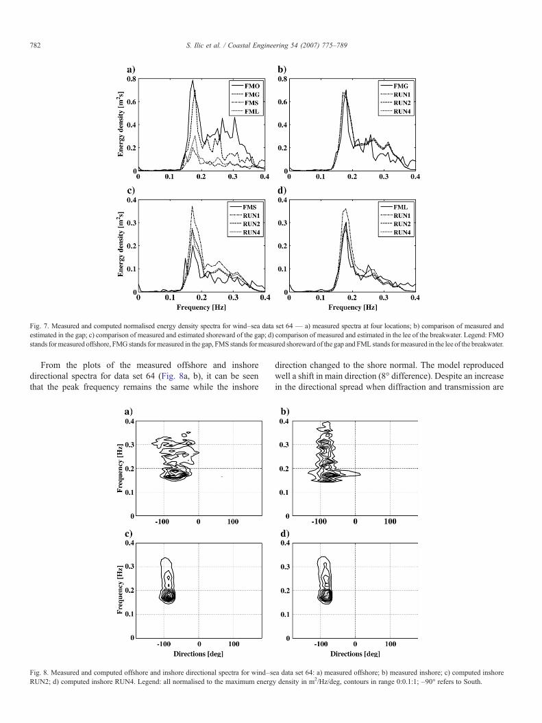
Fig. 7. Measured and computed normalised energy density spectra for wind–sea data set 64 — a) measured spectra at four locations; b) comparison of measured andestimated in the gap; c) comparison of measured and estimated shoreward of the gap; d) comparison of measured and estimated in the lee of the breakwater. Legend: FMOstands formeasured offshore, FMG stands formeasured in the gap, FMS stands formeasured shoreward of the gap and FML stands formeasured in the lee of the breakwater.


From the plots of the measured offshore and inshoredirectional spectra for data set 64 (Fig. 8a, b), it can be seenthat the peak frequency remains the same while the inshore

Fig. 8. Measured and computed offshore and inshore directional spectra for wind–sRUN2; d) computed inshore RUN4. Legend: all normalised to the maximum energ

direction changed to the shore normal. The model reproducedwell a shift in main direction (8° difference). Despite an increasein the directional spread when diffraction and transmission are

ea data set 64: a) measured offshore; b) measured inshore; c) computed inshorey density in m2/Hz/deg, contours in range 0:0.1:1; –90° refers to South.

Fig. 9. Measured and computed normalised energy density spectra for bimodal data set 67— a)measured spectra at four locations; b) comparison ofmeasured and estimatedin the gap; c) comparison of measured and estimated shoreward of the gap; d) comparison of measured and estimated in the lee of the breakwater (legend as in Fig. 7).


included (RUN2, RUN4), it is generally less than half of themeasured values in all tests. Although good agreement isobserved for data sets 69 and 75 (Ilic et al., 2007), the best

Fig. 10. Measured and computed offshore and inshore directional spectra for bimodRUN2; d) computed inshore RUN4 (legend as in Fig. 8).

prediction in the lee of the breakwater was for data set 64. In thiscase the incident waves come from the SE and directly radiateinto the area where the measurements were taken.

al data set 67: a) measured offshore; b) measured inshore; c) computed inshore

Fig. 11. Measured and computed normalised energy density spectra for swell data set 73 — a) measured spectra at four locations; b) comparison of measured andestimated in the gap; c) comparison of measured and estimated shoreward of the gap; d) comparison of measured and estimated in the lee of the breakwater (legend asin Fig. 7).


4.3.2. Bimodal spectraThe frequency spectra for bimodal-sea cases 66 and 67 have

two distinctive peaks at a low frequency of around 0.1 Hz

Fig. 12. Measured and computed offshore and inshore directional spectra for swell datd) computed inshore RUN4 (legend as in Fig. 8).

(swell) and at a high frequency of around 0.2–0.25 Hz (wind–sea). The inshore spectral densities for higher frequencies arereduced whereas there is an increase in spectral densities for

a set 73: a) measured offshore; b) measured inshore; c) computed inshore RUN2;


lower frequencies. There is also a shift of energy density frompeak frequencies to lower neighbouring frequencies. This isillustrated in Fig. 9a for case 67. From comparison plotsbetween the measured and predicted inshore spectra in Fig. 9b,c, d, it can be seen that the shape and the peak frequency of the‘wind spectra’ are well predicted. However, the downwardsshift of the swell peak frequency is not predicted. There is alsoan overestimation of spectral energy densities for higherfrequencies at all locations and an underestimation of theswell energy density in the lee of the breakwater for all tests.

The offshore and inshore measured directional spectra aregiven in Fig. 10a, b. The inshore spectrum is essentially single-peaked whereas the offshore is double peaked. There is a shift ofthe swell peak frequency to lower frequency and a shift indirection to the shore normal in the inshore spectrum. There is alsothe presence of some reflection for the peak frequency inshore,which was not modelled. As seen in Fig. 9 the model did notreproduce the frequency shift but it did reproduce a directionalshift with a 4° difference. Although, the estimated directionalspectra with RUN2 (Fig. 10c) and RUN4 (Fig. 10d) are similar,the directional spreading increased slightly for RUN4. Similardifferences between predicted and measured spectra are observedfor data set 66, not shown here (Ilic et al., 2007).

4.3.3. Swell spectraFor swell cases 72 and 73, most of the energy is contained in

the low frequencies (less than 0.1 Hz). There are considerablechanges in the shape of the frequency spectra between theoffshore and inshore as shown for case 73 (Fig. 11a). Comparison

Fig. 13. Influence of beach reflection on energy density predictions for swell data sespectrum (m2/Hz/deg); d) comparison of measured and predicted frequency dependenLegend: RUNBR stands for sensitivity tests with reflection=0.83 at two grid spacincoefficient, CRC stands for computed frequency dependent reflection coefficient, FM

of predicted and measured spectral energy densities for case 73 atthree locations is given in Fig. 11b, c, d. Spectral energy densitiesare underestimated at all locations with the largest differencefound in the lee of the breakwater. Overall, the differences weresmallest for RUN1. As in the bimodal cases, the model tests donot reproduce the downwards shift in the peak frequency.

Fig. 12a, b shows the measured offshore and inshoredirectional spectra for dataset 73. The offshore spectrum has anarrow frequency and directional spread. Inshore, the peakfrequency is lower than offshore and direction has changedtowards the shore normal, while the directional spread and thereflection increased. The corresponding predicted directionalspectra for RUN2 and RUN4 are given in Fig. 12 c, d. The peakfrequency shift in the inshore is not predicted, but the meandirection is well-predicted, and is best in RUN2 (4° difference).The directional spreading is much lower than measured andtypically less than 1/3 of the measured value for all runs. Thereflection detected inshore (Fig. 12b) is not modelled. Thepredicted frequency and directional spectra for swell dataset 72,not shown here, were much closer to those measured than fordata set 73, despite a mismatch in the peak frequency. Some ofthe observed difference can be associated with the differentnumber of convolution cycles used when predicting data sets 72and 73, which were 6 and 11 respectively.

4.4. Sensitivity tests

Further tests were performed to investigate the inclusion ofbeach reflection, increased wave transmission, friction and currents

t 73: a) shoreward of the gap; b) lee of the breakwater; c) computed directionalt reflection coefficients plotted over normalised measured and predicted spectra.g from the boundary, MRC stands for measured frequency dependent reflectionS and FML as in Fig. 7.


on model predictions. The influence of beach reflection was testedfor data set 73, for which a large amount of reflection had beendetected inshore. The obstacles, as in the case of breakwaterreflection, were implemented at two grid spacing from theshoreward boundary in order to observe the effect of reflection inthe embayment. Three different beach reflection coefficients werechosen: one derived from measurements (0.55) by the expressiongiven in (5) and two of slightly higher values (0.83 detected forpeak frequency and 0.99). By increasing the reflection the predictedwave heights increased in both locations in the embayment.

Fig. 13 shows the results for an average reflection coefficientof 0.83, which is close to the reflection coefficient for thefrequencies containing most of the energy (Fig. 13d). Theinclusion of beach reflection increased the energy at bothmeasurement locations in the embayment (Fig. 13a, b). Also,the reflection can now be clearly seen in the directionalspectrum at the position shoreward of the gap (Fig. 13c). Thesetests proved that beach reflection has an important influence onwave height distributions behind breakwaters, and it would bedesirable to include a frequency dependent reflection coefficientinto the model.

Sensitivity tests were performed with data sets 64 and 73, byincreasing the transmission through the breakwater first to 40%and then 60%. The model results with 20% transmission(RUN4) matched best the measured frequency spectra and waveheights for data set 64. In contrast, the agreement between thecomputed and measured frequency spectra is best for the highertransmission of 60% for data set 73 (Fig. 14a, b). Clearly,frequency dependent transmission coefficients are required tocorrectly model the low frequency case.

Fig. 14. Influence of transmission and tidal currents on energy density predictions forbreakwater; comparison of spectra with and without tidal currents c) in the gap and d)with transmission coefficient 0.4 and 0.6, and with tidal currents, respectively.

Additional sensitivity tests that looked at the influence offriction onmodel predictions (Ilic et al., 2007) showed that frictionhas minor effect for these cases. The role of wave–currentinteraction was examined by including wave-induced and tidalcurrents in the diffraction resolving model SWAN. The wave-induced currents were computed by Delft3D model (Lesser et al.,2004)with the standard settings, as therewere nomeasurements ofthe currents available for calibration. The predicted wave inducedcurrents were rather small (up to 7 cm/s) and did not have asignificant effect on predictedwave height and directional spectra.

Tidal currents were simulated using the tidal current model inDelft3D with boundary conditions obtained from the Conti-nental Shelf Model (CSM) (Gerritsen et al., 1995). The tidalcurrents in the embayment predicted for the periods when thewave measurements were taken were up to 27 cm/s. The wave-tidal current interaction was simulated only for data set 64 and73. Fig. 14c, d shows a comparison between the frequencyspectra, predicted with and without tidal interaction, in the gapand in the lee of the breakwater with the largest tidal currents fordata set 73. Due to tidal interaction, there is a slight increase ofenergy in the gap and decrease of energy in the lee of thebreakwater. A very slight shift of peak frequency and skewingof the spectrum to lower frequencies is observed due to tidalinteraction in the frequency spectra computed in the gap. Also, achange in the peak direction has been detected in the computeddirectional spectrum at the position shoreward of the gap.

In summary the wave height predictions were better for wind–sea than swell–sea conditions. For wind–sea waves with broaddirectional distributions, part of the energy propagates directly intothe shadow zone and is not affected by diffraction processes.

swell data set 73: influence of transmission a) shoreward of the gap; b) lee of thelee of the breakwater. Legend: RUNT1, RUNT2 and RUNTC are sensitivity tests


Besides refraction–diffraction processes, beach reflection andtransmission appear to influence the wave transformation behindthe breakwaters. The model predicted well the shift in the maindirection inshore. However, it failed to predict the shift in the peakfrequency and directional spreading. Simulations with the lumpedtriad approximation (LTA) did not change results (Ilic et al., 2007).

5. Discussion

A detailed comparison of the calculated and measureddirectional spectra for different RUNS can help to elucidate theimportant processes that influence the transformation of directionalwave spectra. It is clear that diffraction processes are lesspronounced for broad directional spectra and hence for sea-waveconditions. Lower-frequency swell waves partially reflect from thesteep upper beach as seen from plots of inshore directional spectra(Fig. 12b). This can cause a spatial modulation of the spectralenergy due to a phase coupling of the incident and reflected waves(Elgar et al., 1997). Reflection from the breakwater andtransmission through the breakwater is more pronounced forlower gravity frequencies, while dissipation on the breakwaters ismore pronounced for higher frequencies (Simmonds et al., 1997;Ilic et al., 2005). Hence, in addition to refraction and diffractionprocesses, reflection from the beach and transmission seem to playa significant role in transformation of swell–sea waves behindbreakwaters. More consideration may need to be given to thefrequency dependent transmission and reflection, and to alternativefrequency dependent wave dissipation in the model.

The wind–sea waves undergo milder transformation than bi-modal or swell waves (Figs. 7a, 9a, 11a). Formoderately energeticswell waves (Hs=0.6–0.8 m), breaking occurs close to the shoreand nonlinear interactions prior to wave breaking could beresponsible for the observed energy shift between frequencies(data set 72 and in particular 73). This corresponds to higherUrsellnumbers at two positions in the embayment for those waves. Theobserved secondary peaks at the harmonics of the spectral peakfrequency can develop due to the non-linear processes duringwave shoaling (Elgar et al., 1993). The very little energy detectedat lower frequencies (e.g. data set 73) can be produced due to theinterference between two neighbouring high-frequency waves inshallow water (Longet-Higgins and Stewart, 1962, Goda, 1975,Guza and Thornton, 1985). Bispectral analysis by Ilic (1999)showed phase coupling of the neighbouring frequency bands,indicating energy transfer between the peak frequency and higherand lower harmonics due to triad interactions. However, theseprocesses have little effect in this study.

In addition, interaction with opposing or following wave-induced and tidal currents can cause change in wave height andalso affect the shape of the frequency spectra (Haller et al., 1997;Ilic et al., 2005). However in this case, wave-induced currents hada very little effect on the wave heights and spectra at the measuredlocation. The stronger tidal currents did have an effect on the shapeof the frequency spectrum, but this does not completely explainthe observed redistribution of energy by frequency. It is interestingthat for all cases with peaks at swell frequencies offshore (data sets66, 67, 72 and 73), the peaks shift downwards to correspond to aperiod of 12.21s inshore. This period is close to a seiching period

of the embayment. Hence, it is possible that seiching of the basinwas occurring at inshore positions, which could affect the shape offrequency spectra. Other minor effects can be caused by processessuch as wave overtopping and local wind.

Although great care was taken when data were measured andanalysed, it is possible that residual measurement errors, instrumentand environmental noise may still have an effect. Inevitably, theremay be errors due to the settings chosen for the model. Furtherlimitations arise from comparison with field measurements at onlythree positions and lack of currents and wind data. The model wastested only for conditions during high tide; and might behavedifferently with rising and falling tidal conditions.

6. Conclusions

In this paper the performance of the new phase-decoupledrefraction–diffraction spectralwavemodelwas assessed in terms ofits ability to predict frequency and directional spectra. The valid-ation of themodel with laboratory data showed that the inclusion ofdiffraction in themodel improved the estimation of wave heights inthe shadow area behind the breakwater. The best agreement wasobserved for the directional spectrum of broad frequency anddirectional distribution, for which diffraction is less pronouncedand also fewer instabilities are introduced due to the diffractionimplementation. Besides the number of convolution cycles in thenumerical solution for diffraction increases for larger L/▵x.

The results of the comparison between themodel and field dataconfirmed that wave heights behind the breakwater are indeedpredicted better when diffraction is included in the model. Waveheights, and the shape of frequency and directional spectra, arebetter reproduced for wind–sea with broad frequency anddirectional spectra than for a swell with narrow frequency anddirectional spectra. In the case of bimodal seas, the ‘sea part’ of thespectra is again better reproduced than the ‘swell part’ of thespectra. For swell waves diffraction processes are more dominantthan for wind–sea waves.

These tests showed the important influence of refraction–diffraction, shoaling and wave dissipation through wave breakingprocesses on the frequency and directional characteristics of wavesaround offshore breakwaters. Beside these processes, reflectionfrom the beach has the most influence on wave height distributionin the embayment for swell and bimodal waves. Transmissionthrough a breakwater influences the wave height in the lee of abreakwater, while both processes influence the directional energydistribution for all sea conditions. The inclusion of frequencydependent transmission and reflection coefficients in the modelwould be desirable. Wave–current interactions and friction hadsecondary roles in this case. However, both linear and non-linearprocesses act simultaneously to alter the frequency and directionalcharacteristics of nearshore waves in particular for swell waves.

It was beyond the capabilities of the model to predict the shiftsin the peak frequency of the spectra for bi-modal and swell waves.The effect of currents, reflection, wave dissipation and non-linearprocesses on these frequency shifts remains uncertain. It ispossible that these apparent shifts are due to basin seiching. Themodel results may need to be compared with results from weaklynonlinear or nonlinear model to resolve these issues. In summary,


the model can accurately predict the transformation of frequencyand directional spectra for wind waves and, with some caution,can be used to predict their transformation for swell waves inintermediate water depths.

Acknowledgment

We would like to thank Professor Marcel Stive who enabledSuzana Ilic's visit to the Faculty of Civil Engineering andGeosciences at Technical University Delft, where this work wasinitiated. Also we would like to thank to Dr Michael Briggs fromthe Coastal and Hydraulics Laboratory, ERDC, Vicksburg, forproviding us with laboratory reports.

References

Axe, P.G., Ilic, S., Chadwick, A.J., 1996. Evaluation of beach modellingtechniques behind detached breakwaters. Proc. of 25th Inter. Conf. onCoastal Engineering, Orlando 1996, USA, ASCE, pp. 2036–2047.

Battjes, J.A., Jansen, J.P.F.M., 1978. Energy loss and set-up due tobreaking of random waves, Proc. 16th Int. Conf. Coastal Engineering,ASCE, pp. 569–587.

Berkhoff, J.C.W., 1972. Computation of combined refraction–diffraction. Proc.13th Coastal Eng. Conf., Vancouver. ASCE, vol. 1, pp. 471–490.

Berkhoff, J.C.W., 1976. Mathematical Models for Simple Harmonic LinearWater Wave Models, Wave Refraction and Diffraction, Phd Thesis, Techn.Univ. of Delft, pp 110.

Booij, N., Ris, R.C., Holthuijsen, L.H., 1999. A third-generation wave model forcoastal regions, Part I, model description and validation. Journal ofGeophysical Research 104 (C4), 7649–7666.

Booij, N., Haagsma, I.J.G., Holthuijsen, L.H., Kieftenburg, A.T.M.M., Ris, R.C.,van der Westhuysen, A.J., Zijlema, M., 2004. SWAN Cycle III version 40.41,User Manual. Delft University of Technology.

Borgman, L.E., 1990. Irregular ocean waves: kinematics and forces. In:LeMehaute, B., Hanes, D.M. (Eds.), Ocean Engineering Science The Sea,Part A, vol. 9. John Wiley and Sons, New York, pp. 1–1301.

Bouws, E., Gunther, H., Rosenthal, W., Vincent, C., 1985. Similarity of the windwave spectrum in finite depth water. Journal of Geophysical Research 90 (C1).

Briggs, M.J., Thompson, E.F., Vincent, C.L., 1995. Wave diffraction aroundbreakwater. Journal of Waterway, Port, Coastal, and Ocean Engineering,ASCE 121 (1), 23–35.

Chadwick, A.J., Ilic, S., Helm-Petersen, J., 2000. An evaluation of directionalanalysis techniques for multidirectional, partially reflected waves: Part 2application to field data. Journal of Hydraulic Research 38 (No 4), 253–259.

Chadwick, A.J., Fleming, C., Simm, J., Bullock, G.N., 1994. Performanceevaluation of offshore breakwaters — a field and computational study.Proceedings Coastal Dynamics 94, ASCE, pp. 950–961.

Chadwick, A.J., Pope, D.J., Borges, J., Ilic, S., 1995. Shoreline directional wavespectra. Part 2. Instrumentation and field measurements. Proc Instn CivEngrs, Water Maritime and Energy, vol. 112 (3).

Davidson, M.A., Bird, P.A.D., Bullock, G.N., Huntley, D.A., 1996. A newdimensional number for the analysis of wave reflection from rubble moundbreakwaters. Coastal Engineering 29, 93–120.

Dingemans, M.W., 1997. Water wave propagation over uneven bottoms, Part 1—linear wave propagation. In: Liu, P.L.F. (Ed.), Advanced Series on OceanEngineering, vol. 13. World Scientific, London.

Dingemans, M.W., Stive, M.J.F., Kuik, A.J., Radder, A.C., Booij, N., 1984.Field and laboratory verification of the wave propagation model CREDIZ.Proc. 19th Int. Conf. on Coastal Engr., Houston, pp. 1178–1191.

Eldeberky, Y., Battjes, J.A., 1996. Spectral modelling of wave breaking:application to Boussinesq equations. Journal of Geophysical Research 101(No C1), 1253–1264.

Elgar, S., Guza, R.T., Freilich, M.H., 1993. Observations of non-linearinteractions in directionally spread shoaling surface gravity waves. Journalof Geophysical Research 98 (C11), 20299–20305.

Elgar, S., Guza, R.T., Raubenheimer, B., Herbers, T.H.C., Gallagher, E., 1997.Spectral evolution of shoaling and breaking waves on a barred beach.Journal of Geophysical Research 102 (C7), 15797–15805.

Frigaard, P., Helm-Petersen, J., Klopman, G., Stansberg, C.T., Benoit, M.,Briggs, M.J., Miles, M., Santas, J., Schaffer, H.A., Hawkes, P.J., 1997.IAHR List of Sea State Parameters — An Update for MultidirectionalWaves, IAHR Seminar Multidirectional Waves and their Interaction withStructures, 27th IAHR Congress, San Francisco, pp. 15–24.

Gerritsen, H., de Vries, J.W., Philippart, M.E., 1995. The Dutch continental shelfmodel. In: Lynch, D.R., Davies, A.M. (Eds.), AGU Coastal and EstuarineStudies, vol. 47, pp. 425–467.

Goda, Y., 1975. Irregular wave deformation in the surf zone. CoastalEngineering in Japan 18, 13–26.

Goda, Y., 1998. An overview of coastal engineering with emphasis on randomwave approach. Coastal Engineering Journal 40 (1), 1–21.

Goda, Y., 2000. Random Seas and Design of Maritime Structures. WorldScientific, Singapore.

Grassa, J.M., 1990. Directional random waves propagation on beaches. Proc.22nd Conf. on Coastal Eng., Delft, pp. 798–811.

Guza, R.T., Thornton, E.B., 1980. Local and shoaled comparisons of sea surfaceelevations, pressures and velocities. Journal of Geophysical Research 85,(3), 1524–1530.

Guza, R.T., Thornton, E.B., 1985. Observations of surf beat. Journal ofGeophysical Research 90 (C2), 3161–3172.

Haller, M.C., Dalrymple, R.A., Svendsen, I.A., 1997. Rip channels andnearshore circulation. Proceedings of ASCE Coastal Dynamics’97,Plymouth, pp. 594–603.

Holthuijsen, L.H., Herman, A., Booij, N., 2003. Phase-decoupled refraction–diffraction for spectral wave models. Coastal Engineering 49, 291–305.

Huntley, D.A., Davidson, M.A., 1998. Estimation of directional waves near areflector. Journal of Waterway, Port, Coastal, and Ocean Engineering, ASCEvol. 124 (6), 1–8.

Hurdle, D.P., Kostense, J.K., Van den Bosch, P., 1989.Mild-slopemodel for thewave behaviour in and around harbours and coastal structures in areas ofvariable depth and flow conditions. Advances in Water Modelling andMeasurement, pp. 307–324.

Ilic, S., Chadwick, A.J., 1995. Evaluation and validation of the mild slopeevolution equation model using field data. Proc. Conf. Coastal Dynamics‘95, Gdainsk, Poland, ASCE, pp. 149–160.

Ilic, S., 1999. Multidirectional Sea Transformation— Field and ComputationalStudy, PhD Thesis, SCSE, University of Plymouth, 1999.

Ilic, S., Chadwick, A.J., Helm-Petersen, J., 2000. An evaluation of directionalanalysis techniques for multidirectional, partially reflected waves: Part 1Numerical investigations. Journal of Hydraulic Research 38 (4), 243–253.

Ilic, S., Chadwick, A.J., Fleming, C., 2005. Detached breakwaters: anexperimental investigation and implication for design — Part1 —hydrodynamics. Proceedings of ICE, Maritime Engineering.

Ilic, S., van der Westhuysen, A.J., Roelvink, J.A., Chadwick, A.J., 2007. Studyof Multidirectional wave transformation around detached breakwaters usingSWAN numerical model, Research Report, Lancaster University, ISBN 978-1-86220-196-5.

Isobe, M., 1987. A Parabolic Model for Transformation of Irregular Waves due toRefraction, Diffraction and Breaking, Coastal Engineering in Japan, Tokyo, vol.30, pp. 33–47.

Lesser, G.R., Roelvink, J.A., van Kester, J.A.T.M., Stelling, G.S., 2004.Development and validation of three-dimensional morphological model.Coastal Engineering 51 (8–9), 883–915.

Li, B., 1994. An evolution equation for water waves. Coastal Engineering 23,227–242.

Li, B., Reeve, D.E., Fleming, C.A., 1993. Numerical solution of the ellipticmild-slope equation for irregular wave propagation. Coastal Engineering 20,85–100.

Longuet-Higgins, M.S., Stewart, R.W., 1962. Radiation stress and mass transportin gravity waves, with application to surf-beats. Journal Fluid Mechanics 13,481–504.

Madsen, P.A., Sørensen, O.R., 1992. A new form of the Boussinesq equationswith improved linear dispersion characteristics. Part 2. A slowly— varyingbathymetry. Coastal Engineering 18, 183–204.


Mory, M., Hamm, L., 1997. Wave, set-up and currents around a detachedbreakwater submitted to regular and randomwave forcing. Coastal Engineering31, 77–96.

O'Reilly, W.C., Guza, R.T., 1991. Comparison of spectral refraction andrefraction–diffraction wave models. Journal of Waterway, Port, Coastal, andOcean Engineering, ASCE 117, 199–215.

Ozkan, H.T., Kirby, J.T., 1993. Evolution of breaking directional spectral wavesin the nearshore zone. Proc., 2nd Int. Symp. On Wave Measurement andAnalysis, Wave’93, New Orleans, pp. 849–863.

Panchang, V.G., Ge, W., Pearce, B.R., Briggs, M.J., 1990. Numerical simulationof irregular wave propagtion over a shoal. Journal of Waterway, Port,Coastal, and Ocean Engineering, ASCE 116 (3), 324–340.

Peregrine, D.H., 1967. Long waves on a beach. Journal of Fluid Mechanics 27,815–827.

Robert West and Partners, 1991. Arun District Council and National RiversAuthority Joint Coastal Defence Study.

Rogers, W.E., Kaihatu, J.M., Petit, H.A.H., Booij, N., Holthuijsen, L.H., 2002.Diffusion reduction in an arbitrary scale third-generation wind wave model.Ocean Engineering 29, 1357–1390.

Simmonds, D.J., Chadwick, A.J., Bird, P.A.D., Pope, D.J., 1997. Fieldmeasurements of wave transmission through a rubble mound breakwater.Proc. Conf. Coastal Dynamics ‘97. ASCE, Plymouth, UK.

Walsh, T.M., 1992. Diffraction of Directional Wave Spectra Around a Semi-Infinite Breakwater, U.S, Army Engineer Waterways Experiment station,Report CERC-92–5.

Wei, G., Kirby, J.T., 1995. Time-dependent numerical code for extendedBoussinesq equations. Journal of Waterway, Port, Coastal, and OceanEngineering 121, 251–261.

Woo, S.B., Liu, P.L.F., 2004. A finite element model for modified Boussinesqequations. Part I: Model development. Journal of Waterway, Port, Coastaland Ocean Engineering, ASCE 130 (1), 1–16.

Zijlema, M., van der Westhuysen, A.J., 2005. On convergence behaviour andnumerical accuracy in stationary SWAN simulations of nearshore windspectra. Coastal Engineering 52, 237–556.

Multidirectional wave transformation around detached breakwaters

Documents