MULTIDIMENSIONAL SEPARATIONS WITH ULTRAHIGH PRESSURE LIQUID CHROMATOGRAPHY – MASS SPECTROMETRY FOR THE PROTEOMICS ANALYSIS OF SACCHAROMYCES CEREVISIAE Kaitlin Michelle Fague A dissertation submitted to the faculty of the University of North Carolina at Chapel Hill in partial fulfillment of the requirements for the degree of Doctor of Philosophy in the Department of Chemistry. Chapel Hill 2014 Approved by: James W. Jorgenson Gary L. Glish R. Mark Wightman Dorothy A. Erie Bo Li

Welcome message from author
This document is posted to help you gain knowledge. Please leave a comment to let me know what you think about it! Share it to your friends and learn new things together.
Transcript

MULTIDIMENSIONAL SEPARATIONS WITH ULTRAHIGH PRESSURE LIQUID
CHROMATOGRAPHY – MASS SPECTROMETRY FOR THE PROTEOMICS
ANALYSIS OF SACCHAROMYCES CEREVISIAE
Kaitlin Michelle Fague
A dissertation submitted to the faculty of the University of North Carolina at Chapel Hill in
partial fulfillment of the requirements for the degree of Doctor of Philosophy in the
Department of Chemistry.
Chapel Hill
2014
Approved by:
James W. Jorgenson
Gary L. Glish
R. Mark Wightman
Dorothy A. Erie
Bo Li

ii
© 2012
Kaitlin Michelle Fague
ALL RIGHTS RESERVED

iii
ABSTRACT
Kaitlin Michelle Fague: Multidimensional Separations with Ultrahigh Pressure Liquid
Chromatography – Mass Spectrometry for the Proteomics Analysis of Saccharomyces cerevisiae
(Under the direction of James W. Jorgenson)
Many biological pathways are controlled by proteins. For proteomics analysis, the peak
capacity of one-dimensional separations is routinely inadequate for the number of components in
a sample. Advances in mass spectrometry (MS) and liquid chromatography (LC) have improved
the limits of detection and sensitivity problems associated with co-elution. However, the pressure
capabilities of the pump on a standard ultrahigh performance LC (UPLC) limit the dimensions of
commercial columns resulting in a maximum peak capacity of 200 in 90 minutes. Various
multidimensional strategies have been developed to further increase the peak capacity.
This dissertation will show the effects of 2DLC prefractionation method and frequency
on proteome coverage. New ultrahigh pressure LC instrumentation with a constant pressure, high
temperature approach for peptide separations is introduced. The system modified a standard
UPLC with a pneumatic amplifier through a configuration of tubing and valves for separations
up to 45000 psi. The modified UHPLC, coupled to a qTOF Premier, produced a peak capacity of
500 in 90 minutes on a meter-long microcapillary column packed with sub-2 micron particles.
Peak capacity plateaued above 800 in 12 hours. The improved prefractionation methodology and
modified UHPLC were coupled for the separation of a model proteome, S. cerevisiae. The
number of protein identifications and coverage improved two-fold as compared to an analogous
separation on the standard UPLC with a commercial column.
iv
ACKNOWLEDGEMENTS
"The most incomprehensible thing about the world is that it is comprehensible."
-Einstein
Paramount in its incomprehensibility is the amount of love that I’ve received to reach this
milestone in my life. Not by luck or anything of my own doing, it is the generosity of my family
and friends that made finishing this experiment in human resilience even possible. First, I would
like to thank my parents and my favorite brother for their encouragement. Constantly introducing
me to new experiences, my parents taught me that there is more to this world than what we see
around us. You encouraged me to venture out on my own. With your support, I knew I was never
truly alone.
To my ever growing family, I thank you all. I come from a long line of hard workers: My
great grandfather travelled to work in intercity Baltimore; my great grandmother canned her own
vegetables to save money; my nanny worked at the A&P; and my pappy loaded trucks at
Westinghouse and Schindler. Their sacrifices and savings have afforded me the opportunity to
pursue my academic aspirations. Their lessons in steadfastness helped me achieve my goals.
These acknowledgements would be incomplete without mentioning the original Doc
Fague (aka JW aka Grandpa) and my wonderful grandma. You have taught me the value of
education. I am honored to earn the title of doctor but will never live up to the original. Cheers!
There are no words worthy of describing my advisor, James W. Jorgenson, and the
amount of support he has given me. I am constantly in awe of your genius. It has been a pleasure
to have you as a mentor. Thank you for your brood of graduate students that have helped me
v
along the way, especially: Laura, Ed, Jordan, Brian, Treadway, Stephanie, Justin and Dan. Thank
you, JJ, for strongly encouraging us to do the things we do not always want to do. Especially,
thank you for demanding that the brightest star of all, Jim Grinias, dance with me. JJ, I can now
leave Carolina with my priceless gem, receive all praises thine.
My many years of scientific education would have meant nothing if it wasn’t for the great
teachers I had in the Shippensburg School District, the Carnegie Mellon University, and the
University of North Carolina. Also, thank you to my mentors at GlaxoSmithKline for the
practical analytical chemistry training and for pulling me when I was struggling. Thank you to
my fellow classmates and coworkers. Your pursuit of excellence made me strive for more.
The business of science could not be completed without my helpful collaborators. This
work has been supported by the Water Corporation. I’d like to thank Theodore Dourdeville for
building the freeze/thaw valve, and Derek Wolfe for designing the switch control circuit
mentioned in Chapter 3. Another thank you goes to Keith Fadgen and Martin Gilar for useful
conversations regarding this work. An analytical chemist is nothing without her working
instrument so thank you to our service engineer, Jim Lekander.
I will conclude with a refrain from one of my favorite musicals, Bob Fosse’s Chicago.
Hopefully, the reader will be singing along after finishing this manuscript:
“Understandable, understandable
Yes it's perfectly understandable
Comprehensible, Comprehensible
Not a bit reprehensible”
It's so defensible.”

vi
TABLE OF CONTENTS
LIST OF TABLES ...................................................................................................................xiv
LIST OF FIGURES ............................................................................................................... xvii
LIST OF APPENDED FIGURES .......................................................................................... xxxi
LIST OF ABBREVIATIONS AND SYMBOLS ................................................................. xxxiii
CHAPTER 1. An Introduction to Differential Proteomics by Multidimensional
Liquid Chromatography-Mass Spectrometry....................................................................1
1.1 Introduction ..................................................................................................................1
1.2 Why study proteomics? .................................................................................................1
1.2.1 Differential proteomics ..........................................................................................2
1.2.2 Differential proteomic tools ...................................................................................3
1.3 Choice of strategy: top-down versus bottom-up .............................................................4
1.3.1 Sample preparation and separation .........................................................................4
1.3.2 Mass spectral detection ..........................................................................................5
1.3.3 Processing proteomics data ....................................................................................6
1.4 Peak capacity ................................................................................................................7
1.4.1 Theory ...................................................................................................................7
1.4.2 The coelution problem ...........................................................................................8
1.4.3 Advent of Ultrahigh Pressure Liquid Chromatography ......................................... 10
1.5 Multidimensional separations ...................................................................................... 10

vii
1.5.1 2D-PAGE ............................................................................................................ 11
1.5.2 MudPIT ............................................................................................................... 11
1.5.3 Top-down proteomics .......................................................................................... 12
1.5.4 Practical peak capacity of 2DLC .......................................................................... 13
1.5.5 Prefractionation.................................................................................................... 14
1.6 Scope of dissertation ................................................................................................... 14
1.7 FIGURES ................................................................................................................... 16
1.8 REFERENCES ........................................................................................................... 27
CHAPTER 2. An Equal-Mass versus Equal-Time Prefractionation Frequency
Study of a Multidimensional Separation for Saccharomyces cerevisiae
Proteomics Analysis ...................................................................................................... 35
2.1 Introduction ................................................................................................................ 35
2.1.1 Peak capacity considerations for multidimensional separations ............................ 35
2.1.2 Top-down versus bottom-up proteomics .............................................................. 37
2.1.3 Prefractionation by Equal-Mass ........................................................................... 38
2.2 Materials and method .................................................................................................. 39
2.2.1 Materials .............................................................................................................. 39
2.2.2 Sample preparation .............................................................................................. 40
2.2.3 Intact protein prefractionation .............................................................................. 41
2.2.4 Protein digestion .................................................................................................. 41
2.2.5 Equal-time fractionation ....................................................................................... 42

viii
2.2.6 Peptide analysis by LC-MS/MS ........................................................................... 42
2.2.7 Equal-mass fractionation ...................................................................................... 43
2.2.8 Peptide data processing ........................................................................................ 43
2.3 Discussion................................................................................................................... 44
2.3.1 Equal-time versus equal-mass fractionation.......................................................... 44
2.3.2 Proteins per fraction ............................................................................................. 46
2.3.3 Venn comparison ................................................................................................. 47
2.3.4 Fractions per protein ............................................................................................ 47
2.3.5 Normalized Difference Protein Coverage ............................................................. 48
2.4 Conclusion .................................................................................................................. 50
2.5 TABLES ..................................................................................................................... 52
2.6 FIGURES ................................................................................................................... 57
2.7 REFERENCES ........................................................................................................... 77
CHAPTER 3. Increasing Peak Capacities for Peptide Separations Using Long
Microcapillary Columns and Sub-2 μm Particles at 30,000+ psi .................................... 80
3.1 Introduction ................................................................................................................ 80
3.1.1 Coupling LC with MS .......................................................................................... 80
3.1.2 Peak capacity improvements ................................................................................ 81
3.1.3 Previous UHPLC systems .................................................................................... 82
3.2 Materials and methods ................................................................................................ 83
3.2.1 Materials .............................................................................................................. 83
ix
3.2.2 Column preparation ............................................................................................. 83
3.2.3 Instrumentation .................................................................................................... 84
3.2.4 Operating procedure ............................................................................................. 85
3.2.5 Gradient volume determination ............................................................................ 85
3.2.6 Gradient linearity determination ........................................................................... 86
3.2.7 Retention time repeatability ................................................................................. 86
3.2.8 Peptide analysis ................................................................................................... 86
3.2.9 Peptide data processing ........................................................................................ 87
3.2.10 Calculating peak capacity ..................................................................................... 87
3.3 Discussion................................................................................................................... 88
3.3.1 Instrumental design .............................................................................................. 88
3.3.2 Gradient storage loop dimensions......................................................................... 89
3.3.3 Selecting the flow rate for gradient loading .......................................................... 90
3.3.4 Repeatability ........................................................................................................ 91
3.3.5 Elevated temperature separations ......................................................................... 91
3.3.6 Column selection ................................................................................................. 92
3.3.7 Separations at ultrahigh pressures......................................................................... 92
3.3.8 Separations with long columns ............................................................................. 94
3.3.9 Separations with smaller particles ........................................................................ 97
3.3.10 Literature comparison .......................................................................................... 99

x
3.4 Conclusions ................................................................................................................ 99
3.5 TABLES ................................................................................................................... 101
3.6 FIGURES ................................................................................................................. 107
3.7 REFERENCES ......................................................................................................... 132
CHAPTER 4. Study of Peptide Stability in RPLC Mobile Phase at Elevated
Temperatures and Pressures ......................................................................................... 136
4.1 Introduction .............................................................................................................. 136
4.2 Materials and method ................................................................................................ 138
4.2.1 Materials ............................................................................................................ 138
4.2.2 Sample stability at elevated pressures and temperatures ..................................... 138
4.2.3 Sample stability at elevated temperatures ........................................................... 139
4.2.4 Peptide data processing ...................................................................................... 140
4.3 Discussion................................................................................................................. 141
4.3.1 Stability testing considerations ........................................................................... 141
4.3.2 Stability at high pressure .................................................................................... 142
4.3.3 Database searching considerations ..................................................................... 142
4.3.4 Venn diagram comparison.................................................................................. 143
4.3.5 Peptide intensity comparison .............................................................................. 144
4.3.6 Temperature degradation study .......................................................................... 145
4.3.7 Sources of analytical variability ......................................................................... 147
4.4 Conclusion ................................................................................................................ 148

xi
4.5 TABLES ................................................................................................................... 149
4.6 FIGURES ................................................................................................................. 154
4.7 REFERENCES ......................................................................................................... 163
CHAPTER 5. Prefractionation Frequency Study with a 32 kpsi UHPLC for the
Multidimensional Separation of the Saccharomyces cerevisiae Proteome .................... 165
5.1 Introduction .............................................................................................................. 165
5.1.1 Prefractionation frequency ................................................................................. 165
5.1.2 Separations at elevated pressures and temperatures ............................................ 166
5.1.3 Orthogonality through prefractionation .............................................................. 167
5.1.4 Equal-mass prefractionation ............................................................................... 168
5.2 Materials and method ................................................................................................ 169
5.2.1 Materials ............................................................................................................ 169
5.2.2 Intact protein prefractionation ............................................................................ 169
5.2.3 Equal-mass fractionation .................................................................................... 169
5.2.4 Protein digestion ................................................................................................ 170
5.2.5 Peptide analysis by UHPLC-MS/MS .................................................................. 171
5.2.6 Peptide data processing ...................................................................................... 172
5.3 Discussion................................................................................................................. 172
5.3.1 Protein identifications ........................................................................................ 172
5.3.2 Analysis time ..................................................................................................... 173
5.3.3 Increased peptide peak intensity ......................................................................... 174

xii
5.3.4 Protein identifications per fractions .................................................................... 174
5.3.5 Protein digestion ................................................................................................ 175
5.3.6 Protein molecular weight distribution ................................................................. 176
5.3.7 Venn diagram comparisons ................................................................................ 177
5.3.8 Fractions per protein .......................................................................................... 178
5.3.9 Protein coverage ................................................................................................ 179
5.4 Conclusions .............................................................................................................. 181
5.5 TABLES ................................................................................................................... 182
5.6 FIGURES ................................................................................................................. 187
5.7 REFERENCES ......................................................................................................... 206
CHAPTER 6. Multidimensional Separations at 32 kpsi using Long
Microcapillary Columns for the Differential Proteomics Analysis of
Saccharomyces cerevisiae ........................................................................................... 209
6.1 Introduction .............................................................................................................. 209
6.2 Materials and method ................................................................................................ 211
6.2.1 Materials ............................................................................................................ 211
6.2.2 Intact protein prefractionation ............................................................................ 212
6.2.3 Equal-mass prefractionation ............................................................................... 212
6.2.4 Protein digestion ................................................................................................ 213
6.2.5 Peptide analysis by UHPLC-MSE ....................................................................... 214
6.2.6 Peptide data processing ...................................................................................... 214

xiii
6.3 Discussion................................................................................................................. 215
6.3.1 Protein prefractionation ...................................................................................... 216
6.3.2 Benefits of increasing second dimension peak capacity ...................................... 217
6.3.3 Increasing protein coverage ................................................................................ 218
6.3.4 Differential proteins ........................................................................................... 219
6.4 Conclusions .............................................................................................................. 223
6.5 TABLES ................................................................................................................... 224
6.6 FIGURES ................................................................................................................. 230
6.7 REFERENCES ......................................................................................................... 238
APPENDIX A. SUPPLEMENTAL DATA FOR CHAPTER 2 ............................................... 243
APPENDIX B. SUPPLEMENTAL DATA FOR CHAPTER 3 ............................................... 251
APPENDIX C. SUPPLEMENTAL DATA FOR CHAPTER 5 ............................................... 260

xiv
LIST OF TABLES
Table 2.1. Chromatographic conditions for the reversed-phase prefractionation of
intact proteins. ............................................................................................................... 52
Table 2.2. Integrated TIC values, summed integrated TIC, and normalized
summed integrated TIC value used to determine first dimension
fractionation schemes. ................................................................................................... 53
Table 2.3. The protein coverage (%) was reported for some of the proteins
involved in S. cerevisiae metabolism. Generally, protein coverage
increased with fractionation frequency. .......................................................................... 55
Table 2.4. The Grand NDPC and Fold-Change in Coverage was listed in for each
fractionation frequency. Positive values represented higher coverage with
the equal-mass fractionation method, and negative values represented
higher coverage with the equal-time fractionation method. The Grand
NDPC and Fold-Change in Coverage favored of the equal-mass method
for 5 and 10. The largest fold-change improvement was 1.4 with the 10
fraction comparison. No significant difference in coverage was observed
between the two methods with 20 first dimension fractions. ........................................... 56
Table 3.1. The methods as programmed into MassLynx were listed along with the
valve timings. The gradient loading time was listed as x, where x equals
the gradient volume divided by the flow rate when loading the gradient.
The time to play back the gradient was listed as y. ....................................................... 101
Table 3.2. The dimensions for each of the analytical columns tested in this
manuscript were listed along with their measured flow rates and
programmed gradient volumes. .................................................................................... 102
Table 3.3. The number of theoretical plates was calculated for several gradient
storage loop internal diameters and gradient volumes. ................................................. 103
Table 3.4. The retention times, in minutes, were listed for several peptides
identified in an enolase digest standatd separated on a 110 cm x 75 µm
column packed with 1.9 µm BEH C18 particles. The gradient volume was
12.5 µL and was repeated 12 times on 12 different days. The retentions
times all had an %RSD of 4.5% or less. ....................................................................... 104
Table 3.5. The average separation window, peak width (4σ), peak capacity, and
number of protein and peptide identifications were listed for each column
at each running condition. ............................................................................................ 105
Table 3.6. The Grand NDPC and Fold-Change Coverage were compared for E.
coli digest separated on the 98.2 cm column run at 30 kpsi to the 44.1 cm
column run at 15 kpsi for three gradient lengths. Positive values
represented higher coverage on the long column, and negative values

xv
represented higher coverage on the shorter column. Grand NDPC and
Fold-Change Coverage increased in favor of the long column as gradient
length increased. .......................................................................................................... 106
Table 4.1. To assess the stability of peptides at elevated pressures and
temperatures, the MassPrep standard protein digest was storage for 10
hours at the conditions listed in this table. .................................................................... 149
Table 4.2. To assess the stability of peptides at elevated temperatures for 2-10
hours, the enolase digest standard was storage at the conditions marked by
an “X” on this table. .................................................................................................... 150
Table 4.3. The number of significantly different peak intensities are listed for the
enolase digest sample stored in 4% mobile phase B at 25, 35, 45, 55, and
65°C for 2, 4, 6, 8, and 10 hours. Intensities were compared to the
unstressed, control sample A in which 19 peptide peaks were identified.
Most of the identified peptide peaks do not have significantly different
intensities when stored at any temperature for 6 hours. After 8 and 10
hours, many more peptides have significantly different intensities. At
these extreme conditions, about 6-7 peaks, or 35% of all identifications,
have significantly different intensities. ......................................................................... 151
Table 4.4. The number of significantly different peak intensities are listed for the
enolase digest sample stored in 40% mobile phase B at 25, 35, 45, 55, and
65°C for 2, 4, 6, 8, and 10 hours. Intensities were compared to the
unstressed, control sample B in which 13 peptide peaks were identified.
Most of the identified peptide peaks do not have significantly different
intensities when stored at any temperature for 6 hours. After 8 hours at
65°C, a couple more peptides have significantly different intensities. At
this extreme condition, two to three peaks, or 19% of all identifications,
had significantly different intensities. .......................................................................... 152
Table 4.5. The retention times and mass-to-charge ratios (m/z) are listed for peaks
that appeared after the enolase digest was stored in the indicated sample
solution. The 199.1 m/z peak appeared when the enolase digest standard
was stored in 4% mobile phase B for extended periods of time above
45°C. This peak is not observed when the sample was stored in 40%
mobile phase B. The other two peaks were degradation products extracted
from the polypropylene microcentrifuge tubes used for sample storage. ....................... 153
Table 5.1. Chromatographic conditions for the reversed-phase prefractionation of
intact proteins. ............................................................................................................. 182
Table 5.2. The fractionation schemes for a set of 20 (a), 10 (b), and 5 (c) first
dimension fractions are listed with the associated first dimension
separation times and the normalized Σ absorbance. ...................................................... 183
xvi
Table 5.3. The method for the second dimension separation at ultrahigh pressure
as programmed into MassLynx is listed along with the valve timings. ......................... 184
Table 5.4. For the separations on the modified UHPLC, the protein coverage (%)
and number of peptides used to identify each protein is reported for the
some of the proteins involved in S. cerevisiae metabolism ........................................... 185
Table 5.5. The Grand NDPC and Fold-Change in Coverage are listed for each
fractionation frequency. Positive values represent higher coverage when
the 110cm long column at 32 kpsi was used for the second dimension
separation as compared to the shorter column run on the standard system.
The Fold-Change in Coverage increased as fractionation frequency
decreased. .................................................................................................................... 186
Table 6.1. Chromatographic conditions for the reversed-phase prefractionation of
intact proteins. ............................................................................................................. 224
Table 6.2. The first dimension prefractionation times of yeast grown on dextrose
and glycerol are listed with the associated normalized Σ absorbance. ........................... 225
Table 6.3. The method for the second dimension separation at ultrahigh pressure,
as programmed into MassLynx, is listed along with the valve timings. ........................ 226
Table 6.4. The protein coverage (%) and number of peptides used to identify each
protein are reported for the some of the proteins involved in S. cerevisiae
metabolism. ................................................................................................................. 227
Table 6.5. The Grand NDPC and Fold-Change in Coverage are listed for each
fractionation frequency. The positive values represent higher coverage
with the 5 equal-mass fractions run on the 110 cm long column at 32 kpsi
as described in this chapter. A negative value would have indicated higher
coverage by our previous results from the 20 equal-time fraction run on
the 25 cm commercial column at 8 kpsi on the standard UPLC.21
The
improvement is small but impressive when one considers that the total
separation time was reduced four fold. ......................................................................... 228
Table 6.6. The T-test confidence value, p-value, fold change, and average
quantitative value was reported for the some of the proteins involved in S.
cerevisiae metabolism. The quantative value was determined as the
Normalized Total Precursor Intensity (x10-³). (*n.d.: Not detected.) ............................. 229

xvii
LIST OF FIGURES
Figure 1.1. The explanation for the flow of genetic information through the
biological system is referred to as the central dogma. DNA is transcribed
into RNA which is translated into proteins. The proteins regulate
metabolites which result in the observed phenotype. ...................................................... 16
Figure 1.2. A small portion of the regulatory pathways involved in S. cerevisiae
metabolism is shown. Proteins in red were up-regulated in yeast grown on
glycerol, and proteins in blue were up-regulated in yeast grown on
dextrose. Small molecules involved in the pathway are in italics. For this
differential study, it is evident that glycerol catabolism, TCA, glyoxylate
cycles are more active for metabolizing glycerol while fermentation and
glycerolneogenesis occurs in dextrose metabolism.26
..................................................... 17
Figure 1.3. A workflow is outlined for a generic proteomics experiment. The
experiment starts with a cell lysate. The analyte is either proteins or
peptides. The sample is separated, commonly by liquid chromatography
(LC), because it has a large loading capacity and peak capacity. LC is
easily coupled to a mass spectrometer. Through electrospray, the
ionization of peptides and proteins is possible making MS a near global
detector. Specificity of MS, based on mass-to-charge, adds another level
of separation. The fragmentation data associated from MS/MS
experiments is useful in identifying the protein. Complex algorithms
process the spectral data to identify peptides and proteins. The relative
abundance, usually in terms of spectral counts, is calculated to give the
fold change in expression of a protein in two differential proteomic
samples.......................................................................................................................... 18
Figure 1.4. Typical work flows for top-down and bottom-up experiments with
considerations for each step are shown. ......................................................................... 19
Figure 1.5. Example spectra of protein envelops acquired by ESI-TOF-MS are
shown drawn to the same intensity scale. Myoglobin and bovine serum
albumin (BSA) were infused in similar amounts. Bovine serum albumin
(a) is 66 kDa and much larger than 17 kDa myoglobin (b). The BSA
molecules are split over more charge states than myoglobin making it less
intense and more difficult to detect. ............................................................................... 20
Figure 1.6. This diagram shows two adjacent peaks, with retention times tr,1 and
tr,1 and peak widths of 4σ at 11% of the maximum height. The two peaks
have a resolution of 1. .................................................................................................... 21
Figure 1.7. This example separation is of a standard enolase protein digest. This
separation has a peak capacity of 100 which is typical for a 30 minute
gradient on a standard UPLC with a commercial column. A peak capacity
of 100 is sufficient for the separation of a single protein digest. ..................................... 22

xviii
Figure 1.8. An example separation (nc=100) of an E. coli digest shows many
overlapping peaks. ......................................................................................................... 23
Figure 1.9. Two instrument schematics are shown for an online multidimensional
separation. In part (a), there are two identical columns (A and B) in the
second dimension. The effluent from the first separation is loaded onto the
head of column A. Using two 4-port valves, the effluent is then switched
to column B, and a gradient is pumped through column A to complete the
second-dimension separation. This cycle continues until the desired
number of fractions from the first dimension is obtained.84
Alternatively,
this can be completed with one second-dimension column using two
storage loops between the dimensions as shown in part (b).80,85
..................................... 24
Figure 1.10. The top-down 2D chromatogram shows S. cerevisiae separated on a
strong anion-exchange column in the first dimension and reversed-phase
column in the second dimension.88
................................................................................. 25
Figure 1.11. The 2D chromatogram shows the bottom-up separation of S.
cerevisiae. A step gradient is implemented for the first dimension
separation. There were five steps dictating the peak capacity of the first
dimension. A reversed-phase column is used in both dimensions. The
separation attempts to be orthogonal by modifying the sample with high-
pH mobile phase in the first dimension and low-pH mobile phase in the
second dimension.88
....................................................................................................... 26
Figure 2.1. This 2D chromatogram was divided in to bins by Davis and
coworkers.7 A perimeter was drawn around the bins containing a circle,
which represented a sample peak, to illustrate the orthogonality of the
separation. ..................................................................................................................... 57
Figure 2.2. The workflow for the prefractionation method started with HPLC-UV
of the intact proteins. Forty fractions were collected, lyophilized, and
digested with trypsin. The forty one-minute-wide fractions were pooled
into 20, 10, and 5 equal-time and equal-mass fractions before the second
dimension analysis by UPLC-MS. The spectral data was searched against
a genomic database to identify the proteins. ................................................................... 58
Figure 2.3. The representative TIC chromatogram from a peptide (second
dimension) separation of the 40 equal-time fraction set showed an
example of peak integration. The peak area was the ∫TIC value used in
Table 2.2 for the determination of the equal-mass prefractionation
schemes. ........................................................................................................................ 59
Figure 2.4. (a) The normalized Σ∫TIC, Σ absorbance, and summed unique protein
count were plotted versus the first dimension separation time and fraction
number. The similarity of the three traces should be noted. The y-axis was
annotated with hash marks in increments of 0.2, 0.1, or 0.05, as shown in

xix
parts (b), (c), and (d), respectively. Lines were drawn from the hash marks
on the y-axis to the corresponding x-coordinate on the normalized equal-
mass curve. These x-coordinates were used to determine size of the first
dimension fractions........................................................................................................ 60
Figure 2.5. The number of protein identifications was plotted versus number of
first dimension fractions. The blue and red traces were for the equal-time
and equal-mass fractionation methods, respectively. The number of
protein identifications increased with increased prefractionation up to 40
fractions. At all prefractionation frequencies, the equal-mass
prefractionation method outperformed the equal-time prefractionation
method. ......................................................................................................................... 61
Figure 2.6. The 2D chromatogram for 40 first dimension fractions was plotted
with the first dimension (protein) separation time and fraction number
plotted on the vertical axes and the second dimension (peptide) separation
on the bottom axis. Starting with fraction 30, the peak pattern repeated for
all subsequent fractions. These peaks corresponded to peptides from
trypsin autolysis. ............................................................................................................ 62
Figure 2.7. The 2D chromatograms for 20 first dimension fractions were plotted
with the first dimension (protein) separation time or fraction number
plotted on the vertical axes and the second dimension (peptide) separation
on the bottom axis. Peak intensity was plotted in the z-direction. In the
later eluting fractions, more peaks were observed in (b) the equal-mass
fractionation chromatogram than in (a) the equal-time fractionation
chromatogram................................................................................................................ 63
Figure 2.8. The 2D chromatograms for 10 first dimension fractions were plotted
with the first dimension (protein) separation time or fraction number
plotted on the vertical axes and the second dimension (peptide) separation
on the bottom axis. Peak intensity was plotted in the z-direction. In the
later eluting fractions, more peaks were observed in (b) the equal-mass
fractionation chromatogram than in (a) the equal-time fractionation
chromatogram................................................................................................................ 64
Figure 2.9. The 2D chromatograms for 5 first dimension fractions were plotted
with the first dimension (protein) separation time or fraction number
plotted on the vertical axes and the second dimension (peptide) separation
on the bottom axis. Peak intensity was plotted in the z-direction. In the
later eluting fractions, more peaks were observed in (b) the equal-mass
fractionation chromatogram than in (a) the equal-time fractionation
chromatogram................................................................................................................ 65
Figure 2.10. The light gray bars show the total protein identifications in each
fraction, and the dark gray bars signify the unique protein identifications
in each fraction for 40 first dimensional fractions. The number of unique

xx
protein identifications decreased in the last 15 fractions faster than the
total protein identifications. This trend was less pronounced as
prefractionation frequency decreased. a) ........................................................................ 66
Figure 2.11. The light gray bars show the total protein identifications in each
fraction, and the dark gray bars signify the unique protein identifications
in each fraction for 20 first dimensional fractions. By more evenly
distributing the sample mass between the fractions, as with the equal-mass
fractionation method (b), the number of unique protein identifications was
more even fraction to fraction and increased in the late eluting fractions as
compared to the equal-time fractionation method (a).a) ................................................. 67
Figure 2.12. The light gray bars show the total protein identifications in each
fraction, and the dark gray bars signify the unique protein identifications
in each fraction for 10 first dimensional fractions. By more evenly
distributing the sample mass between the fractions, as with the equal-mass
fractionation method (b), the number of unique protein identifications was
more even fraction to fraction and increased in the late eluting fractions as
compared to the equal-time fractionation method (a). .................................................... 68
Figure 2.13. The light gray bars show the total protein identifications in each
fraction, and the dark gray bars signify the unique protein identifications
in each fraction for 5 first dimensional fractions. By more evenly
distributing the sample mass between the fractions, as with the equal-mass
fractionation method (b), the number of unique protein identifications was
more even fraction to fraction and increased in the late eluting fractions as
compared to the equal-time fractionation method (a). .................................................... 69
Figure 2.14. Venn diagram (a) showed the overlap in protein identifications for 5,
10, and 20 equal-time fractions. Increasing fractionation to 20 led to new
protein identifications while still identifying most of the proteins identified
in the five and ten fraction sets. Venn diagram (b) showed the overlap in
protein identifications for 20 and 40 equal-time fractions. .............................................. 70
Figure 2.15. The Venn diagram showed the overlap in protein identifications for
5, 10, and 20 equal-mass fractions. Increasing fractionation to 20 led to
new protein identifications while still identifying most of the proteins
identified in the five and ten fraction sets. ...................................................................... 71
Figure 2.16. Fractions per protein described the percentage of protein
identifications that were detected in one, two, or more fractions (3+). As
prefractionation frequency increased, more proteins were identified in
multiple fractions. This effect was heightened for the equal-time fractions
(blue) as compared to the equal-mass fractions (red). ..................................................... 72
Figure 2.17. To compare the 5 equal-mass and 5 equal-time fractions, the
Normalized Difference Protein Coverage (NDPC) was plotted with

xxi
proteins with higher coverage on the left, and proteins with lower
coverage on the right. If a protein was identified with higher sequence
coverage in the 5 equal-mass fractions, its NDPC value was positive (red
bars). The blue bars signified higher coverage in the 5 equal-time
fractions. Differences in coverage were minimal for highly covered
proteins. As protein coverage decreased, more proteins were identified
with higher coverage in the equal-mass fractions. The dashed lines
indicate a level of two-fold greater protein coverage. ..................................................... 73
Figure 2.18. The NDPC compared the equal-mass and equal-time methods for 5
(part a), 10 (part b), and 20 (part c) first dimension fractions. If a protein
was identified with higher sequence coverage in the equal-mass fractions,
the NDPC value was positive (red lines). The blue lines signified higher
coverage in the equal-time fractions. Proteins with higher coverage were
plotted on the left, and proteins with lower coverage were on the right.
Differences in coverage were minimal for highly covered proteins. As
protein coverage decreased, more proteins were identified with higher
coverage by the equal-mass method for 5 and 10 fractions. There was little
difference in NDPC for 20 equal-mass and 20 equal-time fractions. ............................... 76
Figure 3.1. The nanoAcquity was shown with the additional tubing and valves
necessary for separations at 45 kpsi driven by the Haskel pneumatic
amplifier pump. ........................................................................................................... 107
Figure 3.2. The gradient playback time of the UHPLC was monitored by the UV
absorbance of acetone in mobile phase B. The gradient linearity was
improved by using a lower flow rate for gradient loading and employing
the 50 µL ID tubing at the head of the gradient storage loop. ....................................... 108
Figure 3.3. The gradient playback time of the UHPLC was monitored by the UV
absorbance of acetone in mobile phase B and plotted in part (a) for several
different gradient volumes which were noted on the graph. The playback
time of the linear region was plotted versus gradient volume in part (b). A
best fit line had the equation y = 3.33x – 4.19 and R2 value of 0.999. The
inverse slope was 0.300 µL/min which corresponded to flow rate. ............................... 109
Figure 3.4. The retention time residuals were plotted versus run order for several
peptides identified in an enolase digest standard separated on a 110 cm x
75 µm column packed with 1.9 µm BEH C18 particles. The gradient
volume was 12.5 µL and was repeated 12 times on 12 different days. The
variability of retention times was random with the R2 values for a 5
th order
polynomial fit of the residuals ranging between 0.57 and 0.69. .................................... 110
Figure 3.5. The Van Deemter plots with reduced terms of hydroquinone
demonstrate the similarity in column performance for the columns tested
in these experiments. ................................................................................................... 111

xxii
Figure 3.6. Chromatograms of MassPREPTM
Digestion Standard Protein
Expression Mixture 2 were collected for separations with increasing
gradient volume on the 44.1 cm x 75 µm ID column packed with 1.9 µm
BEH C18 particles. Separations were completed at 15 kpsi. The insert of a
representative peptide peak with 724 m/z extracted from all four
chromatograms demonstrated the increase in peak width and decrease in
peak height as the as gradient volume increased. .......................................................... 112
Figure 3.7. Chromatograms of MassPREPTM
Digestion Standard Protein
Expression Mixture 2 were collected for separations with increasing
pressure and flow rate on the 44.1 cm x 75 µm ID column packed with 1.9
µm BEH C18 particles. Separations were completed with a 56 µL gradient
volume. The insert of a representative peptide peak with 724 m/z extracted
from all three chromatograms showed the decrease in peak width and
constant signal intensity as pressure and flow rate increased. ....................................... 113
Figure 3.8. Peak capacity versus separation window was displayed for separations
on a 44.1 cm x 75 µm ID column with 1.9 µm BEH C18 particles. Each
line represented a different running pressure, and each point on a line
(from left to right) represented the gradient profiles of 4, 2, 1, or 0.5
percent change in mobile phase composition per column volume. ................................ 114
Figure 3.9. Chromatograms of MassPREPTM
E. coli Digestion Standard were
collected for separations with increasing gradient volume on the 44.1 cm x
75 µm ID column packed with 1.9 µm BEH C18 particles. Separations
were completed at 15 kpsi. Though the chromatograms were very busy, an
increase in resolution was observed as gradient volume increased which
was indicated by the signal being closer to baseline between two adjacent
peaks. .......................................................................................................................... 115
Figure 3.10. Chromatograms of MassPREPTM
E. coli Digestion Standard were
collected for separations with increasing pressure and flow rate on the 44.1
cm x 75 µm ID column packed with 1.9 µm BEH C18 particles.
Separations were completed with a 56 µL gradient volume. ......................................... 116
Figure 3.11. The peptide and protein identifications for E. coli were plotted versus
the separation window and peak capacity for several separations on a 44.1
cm x 75 µm ID column with 1.9 µm BEH C18 particles. Each line
represents a different running pressure, and each point on a line (from left
to right) represented the gradient profiles of 4, 2, 1, or 0.5 percent change
in mobile phase per column volume. ............................................................................ 117
Figure 3.12. Protein identifications per minute or productivity was plotted for the
E. coli protein identifications from analyses at varying gradient volumes
and pressures on the 44.1 cm x 75 µm ID column with 1.9 µm BEH C18
particles. Productivity was highest for the steepest gradient run at the
highest pressure. .......................................................................................................... 118

xxiii
Figure 3.13. Chromatograms of MassPREPTM
Digestion Standard Protein
Expression Mixture 2 were collected for separations with increasing
pressure on a short and long column. The separation time was similar for
the 98.2 cm x 75 µm ID column and 44.1 cm x 75 µm ID column packed
with 1.9 µm BEH C18 particles. The insert of a representative peptide
peak with 724 m/z extracted from both chromatograms showed the
decrease in peak width and constant signal intensity as pressure and
column length increased. ............................................................................................. 119
Figure 3.14. The increasing peak capacity versus separation window plot
demonstrated the benefit of using higher pressures to run longer columns
in the same amount of time as shorter columns. The red line represented
separations at 15 kpsi on a 44.1 cm x 75 µm ID column with 1.9 µm BEH
C18 particles. The blue line represented separations at 30 kpsi on a 98.2
cm x 75 µm ID column with 1.9 µm BEH C18 particles. The gray line
represented separations on a commercial UPLC with a commercial
column (25 cm x 75 µm ID column with 1.9 µm BEH C18 particles). Each
point on a line (from left to right) represented the gradient profiles of 4, 2,
1, or 0.5 percent change in mobile phase per column volume. ...................................... 120
Figure 3.15. Chromatograms of MassPREPTM
E. coli Digestion Standard were
collected for separations with increasing gradient volume on the 98.2 cm x
75 µm ID column packed with 1.9 µm BEH C18 particles. Separations
were completed at 30 kpsi. Though the chromatograms were very busy, an
increase in resolution was observed as gradient volume increased which
was indicated by the signal being closer to baseline between two adjacent
peaks. These were the shotgun proteomic experiments with the highest
peak capacities. ............................................................................................................ 121
Figure 3.16. This chromatogram of MassPREPTM
E. coli Digestion Standard from
the 98.2 cm x 75 µm ID column packed with 1.9 µm BEH C18 particles is
a zoomed in version of the purple chromatogram in Figure 3.15. The
return of signal to baseline between several adjacent peaks demonstrated
the gain in resolution from using long columns at elevated pressures and
temperature for proteomics analysis. ............................................................................ 122
Figure 3.17. The peptide and protein identifications for E. coli were plotted versus
the separation window in parts a and b, respectively. The red line
represented separations at 15 kpsi on a 44.1 cm x 75 µm ID column with
1.9 µm BEH C18 particles. The blue line represented separations at 30
kpsi on a 98.2 cm x 75 µm ID column with 1.9 µm BEH C18 particles.
The gray line represented separations on a commercial UPLC with a
commercial column (25 cm x 75 µm ID column with 1.9 µm BEH 18
particles). Each point on a line (from left to right) represented the gradient
profiles of 4, 2, 1, or 0.5 percent change in mobile phase per column
volume. ....................................................................................................................... 123
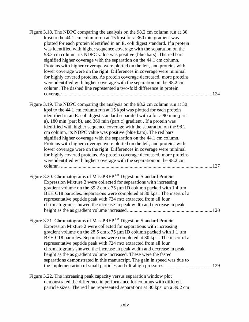
xxiv
Figure 3.18. The NDPC comparing the analysis on the 98.2 cm column run at 30
kpsi to the 44.1 cm column run at 15 kpsi for a 360 min gradient was
plotted for each protein identified in an E. coli digest standard. If a protein
was identified with higher sequence coverage with the separation on the
98.2 cm column, its NDPC value was positive (blue bars). The red bars
signified higher coverage with the separation on the 44.1 cm column.
Proteins with higher coverage were plotted on the left, and proteins with
lower coverage were on the right. Differences in coverage were minimal
for highly covered proteins. As protein coverage decreased, more proteins
were identified with higher coverage with the separation on the 98.2 cm
column. The dashed line represented a two-fold difference in protein
coverage. ..................................................................................................................... 124
Figure 3.19. The NDPC comparing the analysis on the 98.2 cm column run at 30
kpsi to the 44.1 cm column run at 15 kpsi was plotted for each protein
identified in an E. coli digest standard separated with a for a 90 min (part
a), 180 min (part b), and 360 min (part c) gradient . If a protein was
identified with higher sequence coverage with the separation on the 98.2
cm column, its NDPC value was positive (blue bars). The red bars
signified higher coverage with the separation on the 44.1 cm column.
Proteins with higher coverage were plotted on the left, and proteins with
lower coverage were on the right. Differences in coverage were minimal
for highly covered proteins. As protein coverage decreased, more proteins
were identified with higher coverage with the separation on the 98.2 cm
column. ....................................................................................................................... 127
Figure 3.20. Chromatograms of MassPREPTM
Digestion Standard Protein
Expression Mixture 2 were collected for separations with increasing
gradient volume on the 39.2 cm x 75 µm ID column packed with 1.4 µm
BEH C18 particles. Separations were completed at 30 kpsi. The insert of a
representative peptide peak with 724 m/z extracted from all four
chromatograms showed the increase in peak width and decrease in peak
height as the as gradient volume increased. .................................................................. 128
Figure 3.21. Chromatograms of MassPREPTM
Digestion Standard Protein
Expression Mixture 2 were collected for separations with increasing
gradient volume on the 28.5 cm x 75 µm ID column packed with 1.1 µm
BEH C18 particles. Separations were completed at 30 kpsi. The insert of a
representative peptide peak with 724 m/z extracted from all four
chromatograms showed the increase in peak width and decrease in peak
height as the as gradient volume increased. These were the fasted
separations demonstrated in this manuscript. The gain in speed was due to
the implementation of small particles and ultrahigh pressures. ..................................... 129
Figure 3.22. The increasing peak capacity versus separation window plot
demonstrated the difference in performance for columns with different
particle sizes. The red line represented separations at 30 kpsi on a 39.2 cm

xxv
x 75 µm ID column with 1.4 µm BEH C18 particles. The blue line
represented separations on a 98.2 cm x 75 µm ID column with 1.9 µm
BEH C18 particles. The green line represented separations on a 28.5 cm x
75 µm ID column with 1.1 µm BEH C18 particles. The gray line
represented separations on a commercial UPLC with a commercial
column. ....................................................................................................................... 130
Figure 3.23. The peak capacity versus separation window plot compared the
highest peak capacities demonstrated in this manuscript, as obtained with
the 98.2 cm x 75 µm ID column with 1.9 µm BEH C18 particles,
separations on the commercial nanoAcquity and several data sets found in
the literature for separations with long columns and at high pressure
(PNNL24
,Harvard39
). The data presented in this manuscript achieved
higher peak capacities in less time as compared to the literature data. .......................... 131
Figure 4.1. The instrument diagram (a) shows the fluidic configuration for sample
storage at elevated pressures and temperatures. Part (b) shows the fluidic
configuration for gradient/sample loading and sample analysis. For
gradient/sample loading, all valves were opened except the nanoAcquity
vent valve. For sample storage and analysis, all valves were closed except
the nanoAcquity vent valve. The haskel pump and column heater were
regulated to the desired pressure and temperature to stress the sample.
During analysis, the haskel pump and column heater were regulated to 15
kpsi and 30°C. ............................................................................................................. 154
Figure 4.2. These chromatograms were from the analysis of the standard protein
digest stored in the gradient storage loop. Storage conditions are listed
above each chromatogram. .......................................................................................... 155
Figure 4.3. These Venn diagrams show the similarities in peptide identification
for the standard protein digest control sample compared to a replicate
analysis and to analysis of the sample stored at stress conditions.................................. 156
Figure 4.4. The log peptide intensities are plotted comparing two replicate
analyses of the control standard protein digest. The confidence lines drawn
on the graph are used to describe the scatter from the dashed y=x line due
to analytical variability. The formulas for each line and the percent of data
points contained within each set of lines are listed in the legend. ................................. 157
Figure 4.5. The log peptide intensities are plotted for the standard protein digest
stored at 45 kpsi and ambient temperature for 10 hours compared to the
control. As listed in the legend, 95.2% of the data points are contained
within the green lines. This percentage is greater than that expected due to
analytical variability which indicates no change in peptide intensity from
storage at 45 kpsi for 10 hours. .................................................................................... 158

xxvi
Figure 4.6. The log peptide intensities are plotted for the standard protein digest
stored at 65°C and ambient pressure for 10 hours compared to the control.
As listed in the legend, 91.5% of the data points are contained within the
green lines. This percentage is less than that expected due to analytical
variability. Most of the variability occurs from data points falling below
the y=x dashed line which indicates a decrease of intensity for peptides in
the elevated temperature sample. ................................................................................. 159
Figure 4.7. The log peptide intensities are plotted for the standard protein digest
stored at 65°C and 45 kpsi for 10 hours compared to the control. As listed
in the legend, 88.8% of the data points are contained within the green
lines. This percentage is less than that expected due to analytical
variability. Most of the variability occurs from data points falling below
the y=x dashed line which indicates a decrease of intensity for peptides in
the stressed sample. ..................................................................................................... 160
Figure 4.8. These red and blue chromatograms are from the analysis of the
enolase digest control and stress sample stored at 65°C for 10 hours.
Feature A (199.1 m/z) is a degradation peak that appeared when enolase
was stored in 4% mobile phase B at elevated temperatures. The green
chromatogram of mobile phase stored in the polypropylene
microcentrifuge tubes at 65°C for 10 hours shows that peak B (460.4 m/z)
and peak C (780.9 m/z) were extracted from the tube and are not peptide
degradation products. ................................................................................................... 161
Figure 4.9. The intensity is plotted versus storage time for a degradation peak
(199.1 m/z) that appeared when the enolase digest standard was stored in
4% mobile phase B for extended periods of time. This peak appeared
when the sample was stored above 45°C. This peak is not observed when
the sample was stored in 40% mobile phase B. ............................................................ 162
Figure 5.1. The workflow for the prefractionation method started with HPLC-UV
of the intact proteins. Thirty-eight one-minute-wide fractions were
collected, lyophilized, and pooled into 20 equal-mass fractions. The 20
equal-mass fractions were digested and also pooled into 10 and 5 equal-
mass fractions. The set of 20, 10, and 5 equal-mass fractions were
analyzed with a second dimension separation by the modified UHPLC-MS
at 32 kpsi. The spectral data were searched against a genomic database to
identify the proteins. .................................................................................................... 187
Figure 5.2. The normalized ΣAbsorbance trace is plotted versus the first
dimension separation time to determine the equal-mass prefractionation
timings. The y-axis is equally divided into 20 (a), 10 (b), and 5 (c)
fractions. A line is drawn from the Σ Absorbance trace to the x-axis to
determine when to take fractions from the first dimension. The UV
chromatogram is overlaid on these plots to show how the area under the
peaks is relatively equal in every fraction..................................................................... 188

xxvii
Figure 5.3. The number of protein identifications is plotted versus number of first
dimension fractions. The green line is for the prefractionation experiment,
described in this chapter, run on the modified UHPLC at 32 kpsi. As a
comparison, the results from this chapter where superimposed on Figure
2.5 (red and blue traces) for a prefractionation study with a standard
UPLC. The number of protein identifications greatly increased through
use of long columns on the UHPLC. ............................................................................ 189
Figure 5.4. Two-dimensional chromatograms for 20 (a,b), 10 (c,d), and 5 (e,f)
first dimension fractions are plotted with the first dimension (protein)
fraction number versus the second dimension (peptide) separation. Base
peak intensity BPI is plotted in the z-direction. Chromatograms on the left
(a,c,e) are from the modified UHPLCat 32 kpsi with a 110 cm column,
and chromatograms on the right (b,d,f) are run on a standard UPLC at 8
kpsi with a 25 cm commercial column. The same amount of protein was
loaded onto the column in both analyses. The gain in intensity was due to
the decreased peak widths on the longer column. ......................................................... 190
Figure 5.5. On average, more unique proteins were identified per fraction as
prefractionation frequency decreased but total proteins identifications per
fraction remained constant. The light gray bars show the total protein
identifications in each fraction, and the dark gray bars signify the unique
protein identifications in each fraction for 20 (a), 10 (b), and 5 (c) first
dimensional fractions analyzed on the modified UHPLC at 32 kpsi. The x-
axis is the first dimension separation time with the UV absorbance
overlaid in red.............................................................................................................. 191
Figure 5.6. More proteins were identified per fraction when the fractions were run
on the 110 cm column at 32 kpsi (a) as compared to the standard UPLC
(b). The light gray bars show the total protein identifications in each
fraction, and the dark gray bars signify the unique protein identifications
in each fraction for 20 first dimension fractions. .......................................................... 192
Figure 5.7. More proteins were identified per fraction when the fractions were run
on the 110 cm column at 32 kpsi (a) as compared to the standard UPLC
(b).The light gray bars show the total protein identifications in each
fraction, and the dark gray bars signify the unique protein identifications
in each fraction for 10 first dimension fractions. .......................................................... 193
Figure 5.8. More proteins were identified per fraction when the fractions were run
on the 110 cm column at 32 kpsi (a) as compared to the standard UPLC
(b).The light gray bars show the total protein identifications in each
fraction, and the dark gray bars signify the unique protein identifications
in each fraction for 5 first dimension fractions. ............................................................ 194
Figure 5.9. These histograms display the protein molecular weight distributions
for the separations at 32 kpsi (a) and for the separations at 8 kpsi (b). The

xxviii
mass distribution corresponding to the 5, 10 and 20 fractions are portrayed
by the black, gray and white bars, respectively. Proteins were identified
with masses up to 250 kDa. For all methods, the median molecular weight
was 39-40 kDa. For the fractions run at 32 kpsi, the increase in
identifications occurred mostly for lower mass proteins 20-70 kDa. ............................. 195
Figure 5.10. The mass chromatograms for 20 (a,b), 10 (c,d), and 5 (e,f) first
dimension fractions are plotted as protein mass versus first dimension
fraction. The log quantitative value for each protein is plotted in the z-
direction. Chromatograms on the left (a,c,e) are from the modified
UHPLC at 32 kpsi on a 110 cm column, and chromatograms on the right
(b,d,f) are from the standard UPLC at 8 kpsi on a 25 cm commercial
column. ....................................................................................................................... 196
Figure 5.11. Similarities in protein identifications are compared for 5 (a), 10 (b),
and 20 (c) first dimension fractions run on the 110 cm column at 32 kpsi
to fractions run on a standard UPLC. ........................................................................... 197
Figure 5.12. The Venn diagram demonstrates the overlap in protein identifications
for 5, 10, and 20 equal-mass fractions run on the 110 cm column at 32
kpsi.............................................................................................................................. 198
Figure 5.13. Fractions per protein describe the percentage of proteins that were
identified in one, two or more (3+) fractions run on the 110 cm column at
32 kpsi (a) and the standard UPLC (b). As prefractionation frequency
increased, more proteins were identified in multiple fractions. A larger
percentage of the proteins were identified in multiple fractions with the
modified system. The increased identification of proteins across multiple
fractions was mostly likely related to the increased peak intensities in the
second dimension separation........................................................................................ 199
Figure 5.14. To compare the 5 fractions run on the modified system to the 5
fractions run on the standard UPLC, the NDPC is plotted with proteins
with higher coverage on the left, and proteins with lower coverage on the
right. If a protein was identified with higher sequence coverage when
analyzed on the modified UHPLC, its NDPC value is positive (blue bars).
The red bars signify higher coverage in the analysis on the standard
UPLC. Differences in coverage were minimal for highly covered proteins.
As protein coverage decreased, more proteins were identified with higher
coverage from the analysis on the modified UHPLC. The dashed lines
indicate a level of two-fold greater protein coverage. (This was a large
graph and split into multiple parts.) .............................................................................. 200
Figure 5.15. The NDPC plotted here compare proteins identified with the
modified and standard UHPLCs for 5 (a), 10 (b), and 20 (c) first
dimension fractions. If a protein was identified with higher sequence
coverage with the modified UHPLC, the NDPC value is positive (blue

xxix
lines). The red lines signify higher coverage with the standard UPLC.
Proteins with higher coverage are plotted on the left, and proteins with
lower coverage are on the right. More proteins were identified with higher
coverage by with the modified UHPLC. ...................................................................... 205
Figure 6.1. The workflow for the prefractionation method started with HPLC-UV
of the intact proteins. Thirty-eight one-minute-wide fractions were
collected, lyophilized, and pooled into 20 equal-mass fractions. The equal-
mass fractions were digested and pooled into 5 equal-mass fractions
before the second dimension analysis by the modified UHPLC-MS at 32
kpsi. The spectral data was searched against a genomic database to
identify the proteins. .................................................................................................... 230
Figure 6.2. The normalized Σ absorbance, plotted here with the UV
chromatograms, was used to distribute the first dimension separation for
yeast grown on dextrose (a) and glycerol (b) into equal-mass fractions. ....................... 231
Figure 6.3. Two-dimensional chromatograms for yeast grown on dextrose (a) and
glycerol (b) are plotted with the first dimension (protein) fraction number
on the vertical axes and the second dimension (peptide) separation on the
bottom axes. Peak intensity (BPI) is plotted in the z-direction. ..................................... 232
Figure 6.4. The light gray bars show the total protein identifications in each
fraction, and the dark gray bars signify the unique protein identifications
in each fraction for yeast grown on dextrose (a) and glycerol (b) with the
UV chromatogram of the first dimension separation overlaid. ...................................... 233
Figure 6.5. Fractions per protein describe the percentage of protein identifications
that were detected in one, two, three, four, or all five fractions. .................................... 234
Figure 6.6. The overlap in identifications is shown for yeast grown on dextrose
and glycerol. ................................................................................................................ 235
Figure 6.7. The –log10 (p-value) is plotted versus the log2 fold change (a). All
points above the horizontal dashed line represent significantly different
protein quantities with 95% minimum confidence. A negative or positive
fold change is a convention for up-regulation of the protein in yeast grown
on dextrose or glycerol, respectively. All points outside the vertical dashed
lines represent a fold change greater that two. Protein quantity is not
captured in the volcano plot so the log of the quantitative value for all
significantly different proteins is plotted (b). Proteins up-regulated in the
dextrose or glycerol sample are closer to the y-axis or x-axis, respectively.
Points falling along the axis were only identified in the sample
corresponding to that axis. The solid line represents y=x, and the dashed
line represents a fold change of two. ............................................................................ 236
Figure 6.8. Several metabolic pathways of S. cervisiae including glycerol
catabolism, glycerolneogenesis, glycolysis, gluconeogenesis,
xxx
fermentation, TCA cycle, and glyoxylate cycle are depicted with protein
identifiers in blue or red if the protein was up-regulated when yeast was
grown on the dextrose or glycerol media, respectively. Identifiers in black
represent proteins that were identified without a significant difference in
abundance. They gray text shows what metabolite are involved in the
pathways. .................................................................................................................... 237

xxxi
LIST OF APPENDED FIGURES
Appendix A.1. To compare the 10 equal-mass and 10 equal-time fractions, the
Normalized Difference Protein Coverage (NDPC) was plotted with
proteins with higher coverage on the left, and proteins with lower
coverage on the right. If a protein was identified with higher sequence
coverage in the 10 equal-mass fractions, its NDPC value was positive (red
bars). The blue bars signified higher coverage in the 10 equal-time
fractions. Differences in coverage were minimal for highly covered
proteins. As protein coverage decreased, more proteins were identified
with higher coverage in the equal-mass fractions. The dashed lines
indicate a level of two-fold greater protein coverage. ................................................... 243
Appendix A.2. To compare the 20 equal-mass and 20 equal-time fractions, the
Normalized Difference Protein Coverage (NDPC) was plotted with
proteins with higher coverage on the left, and proteins with lower
coverage on the right. If a protein was identified with higher sequence
coverage in the 20 equal-mass fractions, its NDPC value was positive (red
bars). The blue bars signified higher coverage in the 20 equal-time
fractions. Differences in coverage were minimal for highly covered
proteins. For 20 fractions, the NDPC did not favor the equal-mass or the
equal-time fractionation methods. The dashed lines indicate a level of two-
fold greater protein coverage. ...................................................................................... 246
Appendix B.1. The NDPC comparing the analysis on the 98.2 cm column run at
30 kpsi to the 44.1 cm column run at 15 kpsi for a 90 min gradient was
plotted for each protein identified in an E. coli digest standard. If a protein
was identified with higher sequence coverage with the separation on the
98.2 cm column, its NDPC value was positive (blue bars). The red bars
signified higher coverage with the separation on the 44.1 cm column.
Proteins with higher coverage were plotted on the left, and proteins with
lower coverage were on the right. Differences in coverage were minimal
for highly covered proteins. As protein coverage decreased, more proteins
were identified with higher coverage with the separation on the 98.2 cm
column. The dashed line represented a two-fold difference in protein
coverage. ..................................................................................................................... 251
Appendix B.2. The NDPC comparing the analysis on the 98.2 cm column run at
30 kpsi to the 44.1 cm column run at 15 kpsi for a 180 min gradient was
plotted for each protein identified in an E. coli digest standard. If a protein
was identified with higher sequence coverage with the separation on the
98.2 cm column, its NDPC value was positive (blue bars). The red bars
signified higher coverage with the separation on the 44.1 cm column.
Proteins with higher coverage were plotted on the left, and proteins with
lower coverage were on the right. Differences in coverage were minimal
for highly covered proteins. As protein coverage decreased, more proteins
were identified with higher coverage with the separation on the 98.2 cm

xxxii
column. The dashed line represented a two-fold difference in protein
coverage. ..................................................................................................................... 254
Appendix B.3. Chromatograms of MassPREPTM
Digestion Standard Protein
Expression Mixture 2 were collected for separations with increasing
pressure and flow rate on the 39.2 cm x 75 µm ID column packed with 1.4
µm BEH C18 particles. Separations were completed with a 50µL gradient
volume. The insert of a representative peptide peak with 724 m/z extracted
from all three chromatograms showed the decrease in peak width and
constant signal intensity as pressure and flow rate increased. ....................................... 257
Appendix B.4. Chromatograms of MassPREPTM
E. coli Digestion Standard were
collected for separations with increasing gradient volume on the 39.2 cm x
75 µm ID column packed with 1.4 µm BEH C18 particles. Separations
were completed at 30 kpsi. Though the chromatograms were very busy, an
increase in resolution was observed as gradient volume increased which
was indicated by the signal being closer to baseline between two adjacent
peaks. .......................................................................................................................... 258
Appendix B.5. Chromatograms of MassPREPTM
E. coli Digestion Standard were
collected for separations with increasing pressure and flow rate on the 39.2
cm x 75 µm ID column packed with 1.4 µm BEH C18 particles.
Separations were completed with a 50µL gradient volume. .......................................... 259
Appendix C.1. To compare the 10 fractions run on the modified system to the 10
fractions run on the standard UPLC, the NDPC is plotted with proteins
with higher coverage on the left, and proteins with lower coverage on the
right. If a protein was identified with higher sequence coverage when
analyzed on the modified UHPLC, its NDPC value is positive (blue bars).
The red bars signify higher coverage in the analysis on the standard
UPLC. Differences in coverage were minimal for highly covered proteins.
As protein coverage decreased, more proteins were identified with higher
coverage from the analysis on the modified UHPLC. The dashed lines
indicate a level of two-fold greater protein coverage. (This was a large
graph and split into multiple parts.) .............................................................................. 260
Appendix C.2. To compare the 20 fractions run on the modified system to the 20
fractions run on the standard UPLC, the NDPC is plotted with proteins
with higher coverage on the left, and proteins with lower coverage on the
right. If a protein was identified with higher sequence coverage when
analyzed on the modified UHPLC, its NDPC value is positive (blue bars).
The red bars signify higher coverage in the analysis on the standard
UPLC. Differences in coverage were minimal for highly covered proteins.
As protein coverage decreased, more proteins were identified with higher
coverage from the analysis on the modified UHPLC. The dashed lines
indicate a level of two-fold greater protein coverage. (This was a large
graph and split into multiple parts.) .............................................................................. 266

xxxiii
LIST OF ABBREVIATIONS AND SYMBOLS
%A percent mobile phase A
%B percent mobile phase B
∫TIC integrated total ion current
°C degrees Celsius
2D two dimensional
2DLC two-dimensional liquid chromatography
2D-PAGE two-dimensional polyacrylamide gel electrophoresis
A absorbance
Å angstrom
ACN acetonitrile
ACS American chemical society
BEH bridged ethyl hybrid
BPI base peak intensity
BSA bovine serum albumin
cm centimeter
dc column diameter
Dm diffusion in the mobile phase
ESI electrospray ionization
F flow rate
FTICR Fourier transform ion cyclotron resonance
g gram
H2O water

xxxiv
Hcm height equivalent of a theoretical plate
(resistance to mass transfer in the mobile phase)
ID internal diameter
IDs identifications
IEX ion-exchange chromatography
IPA 2-propanol
iTRAQ isobaric-tag-for-relative-and-absolute-quantification
kDa kiloDalton
kpsi kilo pounds per square inch
kV kilovolts
L liter
L length
LC liquid chromatography
LIFO last in first out
M molar
m meter
m/z mass to charge ratio
MALDI matrix assisted laser desorption ionization
mg milligram
min minute
mL milliliter
mM millimolar
mm millimeter
MRM multiple reaction monitoring

xxxv
MS mass spectrometry
MSE mass spectrometry expression
N number of theoretical plates
nc peak capacity
NDPC normalized difference protein coverage
ng nanogram
nL nanoliter
nm nanometer
np practical peak capacity
O.D. optical density
pI isoelectric point
PLGS ProteinLynx Global Server
PLRP-S polystyrene-divinylbenzene reversed-phase HPLC column
Pmax maximum peak capacity
pmol picomole
PPP pentose phosphate pathway
psi pounds per square inch
qTOF quadrapole time-of-flight
Rep replicate
RPLC reversed-phase liquid chromatography
SEC size exclusion chromatography
sec second
SF surfactant

xxxvi
SILAC stable-isotope-labeling-by-amino-acids-in-cell-culture
t time
TCA the citric acid cycle
TCPK tosyl phenylalanyl chloromethyl ketone, chymotrypsin inhibitor
td dead time
TFA trifluoroacetic acid
tg gradient time
TIC total ion current
tm mobile phase time
u linear velocity
UHPLC ultrahigh pressure liquid chromatography
UPLC ultrahigh performance liquid chromatography
UV ultraviolet
V volts
V volume
v/v volume per volume
v:v:v volume to volume to volume ratio
Vis visible
w/w weight per weight
Xg times gravity
YAPG yeast agar peptone glycerol
μg microgram
μL microliter

xxxvii
μm micrometer
Σ∫TIC summed integrated total ion current
ΣA summed absorbance

1
CHAPTER 1. An Introduction to Differential Proteomics by Multidimensional Liquid
Chromatography-Mass Spectrometry
1.1 Introduction
Protein regulation has long been studied to better understand biological processes.1
Analyses of proteins are complicated because there are thousands of proteins in a cell spanning a
large range of abundances (upwards of 1010
).2 A common approach to study protein regulation is
by differential proteomics using multidimensional chromatography to separate the complex
mixture followed by detection with mass spectrometry (MS).3,4
In this introductory chapter, the
need for studying differential protein regulation by multidimensional chromatography-MS will
be explained.5 Several accomplishments made in this field will be reviewed. Building on the
ideas discussed in this introduction, the aim of this dissertation will be to improve the coverage
of a model proteome, Saccharomyces cerevisiae, through the development of separation methods
and instrumentation.
1.2 Why study proteomics?
For many years, scientists have been trying to understand why certain phenotypes are
observed in nature.6,7,8
For example, why do certain populations of people develop diabetes or
heart disease while others do not? Some causes are environmental, such as diet and exercise, but
other causes are inherently biological.9,10
The central dogma (Figure 1.1) is described as the flow
of genetic information through the biological system.11
As the central dogma progresses from
DNA, to RNA, to proteins, and finally metabolites, the complexity increases in both number of
molecules and variety.12
DNA and RNA are made of four nucleotides,13
proteins are made from

2
20 endogenous amino acids,11
and metabolites can be a variety of small molecules including
carbohydrates, lipids, etc.14
As complexity of the biological sample increases, the burden on the
analytical method to study these molecules also increases.15,16,17
Scientists believed that unlocking the genomic code would demystify the existence of
certain phenotypes.18
In the 1990s, the United States government funded the completion of the
human genome.19,20
However, scientists soon learned that not all of the genome is transcribed
into RNA,21
and not all RNA is translated into proteins. Proteins control cellular pathways, and
the metabolites, involved in these pathways actually, account for the phenotype. After
translation, the protein can be further modified with functional groups such as acetate, phosphate,
lipids and carbohydrates. These post-translational modifications (PTMs) extend the function of
the protein.11
For the regulatory role that proteins play in biological pathways, the field of
proteomics emerged.22, 23,24
1.2.1 Differential proteomics
Consider two cell types, with different genetic variants or observed phenotypes.
Determining which proteins are up and down regulated between the two samples can shed light
onto what biological pathways are active. This study of relative protein abundance became
known as differential proteomics.5,25
For example, Figure 1.2. shows a portion of the regulatory
pathways involved in S. cerevisiae (yeast) metabolism.26
Proteins in red were up-regulated in
yeast grown on glycerol, and proteins in blue were up-regulated in yeast grown on dextrose.
From this differential study, it is evident that the citric acid (TCA) and glyoxylate cycles are
more active when metabolizing glycerol, and fermentation is preferred for dextrose metabolism.
Figure 1.2. also shows how many molecules are involved in just a simple biological pathway. In
a simple proteome, such a yeast, there are thousands of proteins to identify spanning a large

3
range of expression levels.27
To tackle these experimental challenges, a need arises to have better
resolution, a large dynamic range and global yet specific detection.28
1.2.2 Differential proteomic tools
Many tools and methods have been developed to study differential proteomics.28
This
chapter aims to highlight some common practices and fundamentally ground breaking
techniques. A generic workflow is outlined in Figure 1.3. The experiment starts with a cell
lysate. The analyte either contains intact proteins or peptides from the digested proteins. The
sample is separated, commonly by liquid chromatography (LC), because it has a large loading
capacity and high resolution.4 Loading capacity is necessary because analysis of a large amount
of total protein may be required to detect a single analyte of low abundance. LC is also easily
coupled to a mass spectrometer. Through electrospray, the ionization of peptides and proteins is
possible making MS the near global detector for proteomics. Specificity of the MS, based on
mass-to-charge, adds another level of separation.4 The fragmentation data, from MS/MS
experiments, are useful in identifying the protein.29,30
The spectral data is compared to a genomic
database, using complex computer algorithms, to identify peptides and proteins.31,32
The relative
abundance, usually in terms of a ratio of spectral counts, is calculated to give the fold change in
expression of a protein in two differential proteomic samples.33
To help with the quantitative analysis of mass spectral data, several common strategies
can be executed such as isobaric-tag-for-relative-and-absolute-quantification (iTRAQ), stable-
isotope-labeling-by-amino-acids-in-cell-culture (SILAC), and label-free.25,34
iTRAQ allows for
absolute quantification by adding an isobaric label to the N-terminus and amine side chains of
peptides. It is used for protein digests of samples collected from biological specimens.35,36
SILAC requires growth of the cells on normal medium for one sample and on an isotopically

4
enriched medium for the other sample. Commonly, arginine labeled with 12
C and 13
C atoms are
used for the normal and enriched media, respectively.37,38
Both iTRAQ and SILAC label the
sample, which greatly reduces analysis time, because differential samples can be pooled prior to
the separation. The spectral data for each sample is deconvoluted by the mass shift due to the
label. Analyzing both samples simultaneously reduces the day-to-day variability that can occur
from temperature changes in the laboratory. The major advantages of label-free relative
quantification are lower cost and a reduced risk of modifying the sample in the labeling process.
Also, the spectra are not busy with isobaric and isotopic data. The validity of quantification
based on spectral counts with the label-free method has been demonstrated in the literature.39,40,41
1.3 Choice of strategy: top-down versus bottom-up
1.3.1 Sample preparation and separation
The first step in analyzing proteomics samples is to decide between a top-down (protein)
or bottom-up (peptide) strategy.30
Typical work flows with considerations for each step are
shown in Figure 1.4. The top-down experiment begins with the separation of intact proteins. A
single protein may exist in many different isoforms and have different post-translational
modifications which would contribute to band broadening.42
Maintaining the solubility of
proteins outside of the cell is difficult.43
Low solubility has limited the development of new
technology for the separation of intact proteins.44
For this reason, many scientists prefer to do a
bottom-up experiment in which the proteins are enzymatically digested, into peptides prior to
analysis.39
Trypsin, the most commonly used digest enzyme, cleaves proteins on the C-terminal
side of arginine and lysine residues creating peptides about 20 amino acids in length.45
Proteins
come in a variety of masses but an average protein sequence would have around 400 amino
acids, and roughly 20 predicted peptides.46
The sample is now soluble but more complex.

5
1.3.2 Mass spectral detection
After the separation, the analytes are introduced into the mass spectrometer. Mass
spectrometry of large biological molecules remained elusive until the invention of matrix
assisted laser desorption ionization (MALDI) and electrospray ionization (ESI). For MALDI, the
matrix is ablated with a laser initiating desorption and ionization of the analyte. The resulting
spectrum, obtained with a time-of-flight (TOF) mass analyzer, contains predominantly singly
charged ions with large peak widths contributing to low resolution (R=m
m, typically 300-400 for
proteins).47,48
ESI has become the preferred source due to its easy coupling with LC where a high
voltage electric field is applied to a narrow capillary. The liquid becomes a fine aerosol, and ions
are completely desolvated before entering the MS.49
The spectrum, from an ESI-TOF-MS,
contains multiply charged ions and has a higher resolution than MALDI (R=50000).50
With the
ability to analyze peptides and proteins by MS, the sample components don’t have to be
completely separated by LC because the MS can detect many species in a single scan.
Furthermore, the development of gas phase ion mobility adds the option of a post-ionization
separation without adding to the total analysis time.51
However, ionization suppression and
matrix effects still plague mass spectrometric techniques, necessitating separation prior to
analysis.52,53
The ESI spectral data from top-down experiments are complex due to the many charge
states of intact proteins.54
Example spectra, drawn on the same intensity scale, are shown in
Figure 1.5. Myoglobin and bovine serum albumin (BSA) were infused in similar amounts.
Bovine serum albumin (a) is 66 kDa and much larger than 17 kDa myoglobin (b). The BSA
molecules are distributed over more charge states than myoglobin making it less intense and

6
more difficult to detect. In contrast, the spectra are less convoluted for a bottom-up experiment
because peptides are generally only detected in the +2 charge state.51
In the MS, it is useful to fragment the parent ion into a series of y- and b- product ions to
identify the protein, as was pioneered by the McLafferty group.29
Due to the size of the analyte,
the fragmentation efficiency is not as great for proteins as it is for peptides.55
For top-down
experiments, higher energy fragmentation, such as collision-induced dissociation (CID) is
popular. For bottom-up experiments, electron-capture dissociation (ECD) or electron-transfer
dissociation (ETD) can provide a more complete fragmentation of the peptide backbone and tend
to retain labile post-translational modifications (PTMs).56
High resolution instruments, such as
orbitraps and FTICR, are required for many top-down experiments.57,58
Until recently, the
acquisition of these mass spectrometers was cost prohibited in many laboratories making the
time of flights instruments, used in bottom-up experiments, more common.59
1.3.3 Processing proteomics data
Finally, the spectral data is processed on a high-performance computer to identify the
proteins. For top-down experiments, the native mass, as it existed in the cell, is deconvoluted
from the parent ion scan.60
For bottom-up experiments, the protein mass is calculated from the
amino acid sequence listed in a genomic database. 31,32,61
An inference problem occurs with the
rebuilding of a protein from the fragmentation data.62
The same peptide sequence may exist in
two different proteins, and it is difficult to determine to which protein the peptide should be
assigned. This is particularly troublesome when the peptide has a PTM. The assignment of a
PTM to a particular protein can be unclear. The inference problem is greater for bottom-up
experiments because peptides from a single protein are spread throughout the entire

7
chromatogram. For a top-down experiment, the protein is fragmented in the MS so all data
pertaining to that protein is contained in a single spectrum.58
Even with these challenges in data processing, the bottom-up approach is a more
common practice largely due to the greater solubility of protein digests.63
It is reported that more
proteins are identified in bottom-up experiments than top-down experiments. For example, the
Coon Lab recently reported the identification of 3,977 yeast proteins in a one hour bottom-up
analysis.41
Larger mass proteins are also identified by bottom-up methods. Based on the amount
of data garnered, a bottom-up approach may be a better option with today’s technology.
However, some scientists argue that a top-down experiment gives a clearer picture of proteins as
they exist in the cell. Improvements to separation science and mass spectrometry are necessary to
make the top-down approach a more common laboratory practice.58
1.4 Peak capacity
1.4.1 Theory
Due to the complexity of proteomics samples, separation of the components is necessary
before identification and quantification of individual proteins. A common way to describe the
quality of a separation is through peak capacity (nc), which is the number of peaks that can be
resolved in a defined separation window.64,65
Throughout this dissertation, the peak width refers
to the width at 4σ. The separation time refers to gradient time (tg) or the time between the first
and last eluting peak. The formula for peak capacity is as follows:
nc radient Time (tg)
Peak Width (4σ) 1 (1-1)
The 4σ peak width refers to the width of the peak at about 11% of the maximum peak
height. If two adjacent peaks, with retention times tr1 and tr2, overlap at 11% of the maximum
height, they have a resolution of 1.66
A formula for resolution (Rs) is shown below:

8
s tr2-tr1
2(σ1 σ2) (1-2)
Now, let t be the point of overlap. If the full peak width is 4σ at the point of overlap, the
mean-retention-time (tr) for each peak is shifted from t by 2σ i.e. half the peak width. A diagram
of this relationship can be found in Figure 1.6. The derivation proving unity resolution is as
follows:
tr,1 t-2σ (1-3)
tr,2 t 2σ (1-4)
s (t 2σ)-(t-2σ)
2(σ1 σ2)
4σ
2(σ1 σ2) (1-5)
Assuming σ1 σ2, (1-6)
s 4σ
4σ 1 (1-7)
An example separation of a standard enolase protein digest is shown in Figure 1.7. This
separation had a peak capacity of 100 which is typical for a 30 minute gradient on a standard
UPLC with a commercial column. A peak capacity of 100 is sufficient for the separation of
peptides from the digest of a single protein.
1.4.2 The coelution problem
Now, consider the same separation method for a bottom-up proteomics sample, such as
the Escherichia coli digest, in Figure 1.8. As evident from the many overlapping peaks, a larger
peak capacity than 100 is necessary. Davis and Giddings67
derived a formula relating the peak
capacity to the percentage of resolved peaks (α):
α -1
2ln (
s
m) (1-8)

9
where m is the number of detectable components in a sample, s is the number of
component peaks separated with a resolution of one or greater, and α is the saturation factor
which is divided by nc.
To apply this relationship to the E. coli digest, the number of detectable components is
related to the 4,000 proteins encoded in its genomic sequence.68
While it is true that not every
protein encoded in the genome is expressed, E. coli is a simple organism so 4,000 proteins is a
conservative value. For example, Homo sapiens (human) has more than 20,000 genes that
encode proteins, and Mus musculus (laboratory mouse) has 30,000 protein encoding genes.69
For
a bottom-up experiment, the proteins would be digested by trypsin into peptides. As mentioned
earlier, the number of digestion sites and peptides varies from protein to protein.46
To make a
very conservative generalization, the number will be estimated at 10 digest peptides per protein.
Therefore, the number of detectable components in a bottom-up sample of E. coli would be
40,000 peptides. Also, assume that the analyst wants 90% of the peaks to have a resolution of
one, i.e.:
s
m . (1-9)
To calculate the peak capacity necessary for a bottom-up separation of E. coli, these
values are plugged into Equation 1-8.
α m
nc
4
nc (1-10)
α -1
2ln( . ) (1-11)
4
nc -
1
2ln( . ) (1-12)
nc 6 , (1-13)

10
There is no single separation that exists with the peak capacity necessary to separate 90%
of the components in an E. coli proteome digest with the resolution of one.
1.4.3 Advent of Ultrahigh Pressure Liquid Chromatography
A major improvement to the separation of proteomic samples has been the invention of
the UHPLC by the Jorgenson group.70
At the time of publishing, the Jorgenson lab reported a
peak capacity of 300 in 30 minutes which more than doubled the peak capacity achieved with a
HPLC.71
This technology was commercialized (as UPLC) 10 years ago and has become a
common instrument in proteomics laboratories. UHPLC enabled the use of microcapillary
columns with sub-2 micron particles which have greater peak capacity than standard bore
columns. Other labs have since reported higher peak capacities through the use of longer
columns.72,73
Chapter 3 of this dissertation has a more in-depth discussion on the benefits of long
microcapillary columns and details a modified UHPLC that produces peak capacities greater
than those previously reported in the literature.
1.5 Multidimensional separations
Even with the highest performing UHPLC, the peak capacity is still not sufficient for
proteomics samples.74
A solution for providing more peak capacity has been multidimensional
separations. Giddings wrote that the peak capacity of a two-dimensional separation is the product
of the two individual peak capacities:
nc,total = nc,1 x nc,2 (1-14)
if (1) the separations are orthogonal and (2) resolution is not lost in coupling the
separations.64

11
1.5.1 2D-PAGE
Traditionally, 2D separations of intact proteins were completed in space via
polyacrylamide gel electrophoresis (2D-PAGE).75,76
In this technique, the sample is first
separated by isoelectric point (pI) and then by molecular weight. The spots are then excised,
digested, and analyzed by MALDI-MS. Both of iddings’ rules are preserved and thousands of
proteins can be separated by this technique, but several limitations exist. (1) Hydrophobic
proteins may not enter the gel. (2) It is labor intensive to excise and digest spots. (3) Resolution
is not as great for proteins with acidic or basic pI as it is for proteins with intermediate pI. (4)
Proteins of low abundance are not easily detected with most staining techniques.77,78
The limitations with 2D-PAGE have led to the development of 2D separations in time via
liquid chromatography (2DLC). oing back to iddings’ second rule for 2D separations, the
multiplicative peak capacity is only achieved if the resolution is preserved from the first to
second dimension.79
For resolution to be preserved, the second dimension would have to be
faster than practically possible in LC, or the first dimension would have to be extremely slowed
down. Therefore, fractionation of the first dimension is often necessary when coupling two
columns. The peak capacity of the first dimension then becomes the number of fractions. In
order to reduce the loss of peak capacity caused by fractionation, the second dimension should
have the greater peak capacity of the two separations.80,81
1.5.2 MudPIT
A common 2DLC method developed by Yates and colleagues is called multidimensional
protein identification in time (MudPIT). This method utilizes a biphasic column in which the
stationary phase for each dimension is packed sequentially into a single column. A step gradient
associated with the first dimension separation mode is run through the column. Between each

12
step, a linear gradient associated with the second dimension separation mode is run. The column
effluent is sent to the MS/MS for detection. Usually, the first mode of separation is strong cation
exchange followed by a second dimension reversed-phase separation.82,83
This method was
developed for protein digests from cell lysates.
1.5.3 Top-down proteomics
The multidimensional separation of intact proteins has occurred online and offline. Figure
1.9.a. shows the instrument schematic for an online approach. There are two identical columns
(A and B) in the second dimension. The effluent from the first separation is loaded onto the head
of column A. Using two 4-port valves, the effluent is then switched to column B, and a gradient
is pumped through column A to complete the second-dimension separation. This cycle continues
until the desired number of fractions from the first dimension is obtained.84
Alternatively, this
can be completed with one second-dimension column using two storage loops between the
dimensions as shown in Figure 1.9.b.80,85
More recent work, associated with the Human Genome Project, focused on an offline
separation of intact proteins by three modes before analysis by ESI-FTICR-MS. The first two
separations were similar to 2D-PAGE because they involved electrophoretic separations by size
and isoelectric focusing. This modern technique used Gel-Eluted Liquid Fraction Entrapment
Electrophoresis (GELFrEE). The proteins are separated on a gel cartridge, migrated off the gel,
and fractionated into a gel-free sample-well. The fraction is isolated in-solution which is easier
than the manual excision required by its slab-gel ancestor. The third mode of separation was
reversed-phase LC. The multidimensional separation took more than 45 hours and identified
1,043 gene products from human cells.55,58

13
1.5.4 Practical peak capacity of 2DLC
In reality, iddings’ rules, for two dimensional peak capacities, are never fully met. The
practical peak capacity is calculated by modifying iddings’ rule with factors that describe the
lack of orthogonality and loss of resolution in the coupling of two separations.86,87
To
demonstrate the practical peak capacity of a real separation, consider the top-down 2D
chromatogram in Figure 1.10. of S. cerevisiae.88
The sample was separated on a strong anion-
exchange column in the first dimension and reversed-phase column in the second dimension.
Resolution is lost in the coupling of the two dimensions. Due to online fractionation, the peak
capacity of the first dimension is reduced to 30. Also, the 2D space is not completely utilized.
The top left of the chromatographic space contains few peaks. This chromatogram also
demonstrates the difficulty of separating intact proteins. The peaks are several minutes wide and
“ghost” as evident from the feature that appears at 1 minutes in fractions 12-25. “ hosting”
describes an analyte that partially remains on the column after the separation method is
complete. The analyte slowly bleeds off the column creating “ghost” peaks in subsequent
chromatograms. In practice, only a portion of the multiplicative peak capacity, described by
Giddings, is realized.
Now, consider the practical peak capacity of the bottom-up 2D chromatogram in Figure
1.11. of S. cerevisiae.88
A step gradient is implemented for the first dimension separation. There
are five steps dictating the peak capacity of the first dimension. A reversed-phase column is used
in both dimensions. The separation attempts to be orthogonal by modifying the sample with
high-pH mobile phase in the first dimension and low-pH mobile phase in the second dimension.
Stapels and Fadgen have demonstrated that this technique has some orthogonal attributes.89
However, the orthogonality leaves a lot to be desired, as evident by the chromatograms in Figure

14
1.11. There are few late eluting peaks in the first fraction (red) and few early eluting peaks in the
last fraction (pink).
1.5.5 Prefractionation
Another offline multidimensional separation has been growing in popularity. This
prefractionation method takes advantage of both top-down and bottom-up experiments.90,91
The
first dimension is an intact protein separation. Fractions of the effluent are collected,
enzymatically digested, and analyzed by reversed-phase UPLC-MS/MS. By changing the sample
from protein to peptide via digestion between the two dimensions, the separations are orthogonal
even if the same separation mode is used in both dimensions. The prefractionation separations
are more orthogonal than the example top-down and bottom-up 2D chromatograms in Figure
1.10 and Figure 1.11. To see example prefractionation chromatograms, refer to Figure 2.7. in
Chapter 2.
1.6 Scope of dissertation
The scope of this dissertation is to improve the separation of proteomic samples through
the development of new liquid chromatography methods and instrumentation. Chapter 2 has a
deeper discussion on the benefits of the protein prefractionation method. It studies how different
prefractionation techniques and frequencies affect the number of protein identifications.
Chapter 3 and 4 demonstrate the peak capacity gained by modifying a UHPLC for separations at
elevated temperatures and pressures. The modified UHPLC is used to improve the productivity
(protein identifications / time) of a prefractionation experiment in Chapter 5. The final chapter
applies the methods developed in the previous chapters to conduct a differential analysis of
S. cerevisiae grown on two different carbon sources. The benefits of these studies are
demonstrated by the improved proteome coverage as compared to previous analyses.

15
The ideas presented in this dissertation can be used, in the future, to analyze other
complex biological samples. As more is discovered about the transmission of biological
information through the central dogma, an interest is metabolomics has grown.92
The
instrumentation described in this dissertation has the potential for metabolomic applications. In
reality, a panomics approach, covering genomics, transcriptomics, proteomics, and
metabolomics, will likely be necessary to fully understand the regulation of biological
pathways.93

16
1.7 FIGURES
Figure 1.1. The explanation for the flow of genetic information through the biological system is
referred to as the central dogma. DNA is transcribed into RNA which is translated into proteins.
The proteins regulate metabolites which result in the observed phenotype.

17
Figure 1.2. A small portion of the regulatory pathways involved in S. cerevisiae metabolism is
shown. Proteins in red were up-regulated in yeast grown on glycerol, and proteins in blue were
up-regulated in yeast grown on dextrose. Small molecules involved in the pathway are in italics.
For this differential study, it is evident that glycerol catabolism, TCA, glyoxylate cycles are more
active for metabolizing glycerol while fermentation and glycerolneogenesis occurs in dextrose
metabolism.26

18
Figure 1.3. A workflow is outlined for a generic proteomics experiment. The experiment starts
with a cell lysate. The analyte is either proteins or peptides. The sample is separated, commonly
by liquid chromatography (LC), because it has a large loading capacity and peak capacity. LC is
easily coupled to a mass spectrometer. Through electrospray, the ionization of peptides and
proteins is possible making MS a near global detector. Specificity of MS, based on mass-to-
charge, adds another level of separation. The fragmentation data associated from MS/MS
experiments is useful in identifying the protein. Complex algorithms process the spectral data to
identify peptides and proteins. The relative abundance, usually in terms of spectral counts, is
calculated to give the fold change in expression of a protein in two differential proteomic
samples.

19
Figure 1.4. Typical work flows for top-down and bottom-up experiments with considerations for
each step are shown.

20
a) Bovine Serum Albumin 66 kDa
m/z b) Myglobin 17 kDa
m/z
Figure 1.5. Example spectra of protein envelops acquired by ESI-TOF-MS are shown drawn to
the same intensity scale. Myoglobin and bovine serum albumin (BSA) were infused in similar
amounts. Bovine serum albumin (a) is 66 kDa and much larger than 17 kDa myoglobin (b). The
BSA molecules are split over more charge states than myoglobin making it less intense and more
difficult to detect.

21
Figure 1.6. This diagram shows two adjacent peaks, with retention times tr,1 and tr,1 and peak
widths of 4σ at 11% of the maximum height. The two peaks have a resolution of 1.

22
Figure 1.7. This example separation is of a standard enolase protein digest. This separation has a
peak capacity of 100 which is typical for a 30 minute gradient on a standard UPLC with a
commercial column. A peak capacity of 100 is sufficient for the separation of a single protein
digest.

23
Figure 1.8. An example separation (nc=100) of an E. coli digest shows many overlapping peaks.

24
a)
b)
Figure 1.9. Two instrument schematics are shown for an online multidimensional separation. In
part (a), there are two identical columns (A and B) in the second dimension. The effluent from
the first separation is loaded onto the head of column A. Using two 4-port valves, the effluent is
then switched to column B, and a gradient is pumped through column A to complete the second-
dimension separation. This cycle continues until the desired number of fractions from the first
dimension is obtained.84
Alternatively, this can be completed with one second-dimension column
using two storage loops between the dimensions as shown in part (b).80,85

25
Top-Down Separation
Figure 1.10. The top-down 2D chromatogram shows S. cerevisiae separated on a strong anion-
exchange column in the first dimension and reversed-phase column in the second dimension.88

26
Bottom-Up Separation Nano2D Hi-Low pH
Figure 1.11. The 2D chromatogram shows the bottom-up separation of S. cerevisiae. A step
gradient is implemented for the first dimension separation. There were five steps dictating the
peak capacity of the first dimension. A reversed-phase column is used in both dimensions. The
separation attempts to be orthogonal by modifying the sample with high-pH mobile phase in the
first dimension and low-pH mobile phase in the second dimension.88

27
1.8 REFERENCES
1. Pandey, A.; Mann, M., Proteomics to study genes and genomes. Nature 2000, 405
(6788), 837-846.
2. Anderson, N. L.; Anderson, N. G., The Human Plasma Proteome: History, Character, and
Diagnostic Prospects. Molecular & Cellular Proteomics 2003, 2 (1), 50.
3. Monteoliva, L.; Albar, J. P., Differential proteomics: An overview of gel and non-gel
based approaches. Briefings in Functional Genomics & Proteomics 2004, 3 (3), 220-239.
4. Righetti, P. G.; Campostrini, N.; Pascali, J.; Hamdan, M.; Astner, H., Quantitative
proteomics: a review of different methodologies. Eur J Mass Spectrom (Chichester, Eng)
2004, 10 (3), 335-48.
5. Roy, S. M.; Anderle, M.; Lin, H.; Becker, C. H., Differential expression profiling of
serum proteins and metabolites for biomarker discovery. International Journal of Mass
Spectrometry 2004, 238 (2), 163-171.
6. Lockhart, D. J.; Winzeler, E. A., Genomics, gene expression and DNA arrays. Nature
2000, 405 (6788), 827-836.
7. Hieter, P.; Boguski, M., Functional genomics: it's all how you read it. Science 1997, 278
(5338), 601-602.
8. e, H.; Walhout, A. J. M.; Vidal, M., Integrating ‘omic’ information: a bridge between
genomics and systems biology. Trends in Genetics 2003, 19 (10), 551-560.
9. Pate, R. R.; Pratt, M.; Blair, S. N.; et al., Physical activity and public health: A
recommendation from the centers for disease control and prevention and the american
college of sports medicine. JAMA 1995, 273 (5), 402-407.
10. Pearson, T. A.; Mensah, G. A.; Alexander, R. W.; Anderson, J. L.; Cannon, R. O.; Criqui,
M.; Fadl, Y. Y.; Fortmann, S. P.; Hong, Y.; Myers, G. L., Markers of inflammation and
cardiovascular disease application to clinical and public health practice: a statement for
healthcare professionals from the centers for disease control and prevention and the
American Heart Association. Circulation 2003, 107 (3), 499-511.
11. Bettelheim, F.; Brown, W.; Campbell, M.; Farrell, S.; Torres, O., Introduction to Organic
and Biochemistry. Cengage Learning: 2012.
12. Crick, F., Central dogma of molecular biology. Nature 1970, 227 (5258), 561-563.
13. Watson, J. D.; Crick, F. H., Molecular structure of nucleic acids. Nature 1953, 171
(4356), 737-738.
14. Schreiber, S. L., Small molecules: the missing link in the central dogma. Nature chemical
biology 2005, 1 (2), 64-66.
28
15. Xiayan, L.; Legido-Quigley, C., Advances in separation science applied to
metabonomics. ELECTROPHORESIS 2008, 29 (18), 3724-3736.
16. Lay Jr, J. O.; Liyanage, .; Borgmann, S.; Wilkins, C. L., Problems with the “omics”.
TrAC Trends in Analytical Chemistry 2006, 25 (11), 1046-1056.
17. Ryan, D.; Robards, K., Metabolomics: the greatest omics of them all? Analytical
Chemistry 2006, 78 (23), 7954-7958.
18. Collins, F. S.; McKusick, V. A., Implications of the human genome project for medical
science. JAMA 2001, 285 (5), 540-544.
19. Sawicki, M. P.; Samara, G.; Hurwitz, M.; Passaro Jr, E., Human Genome Project. The
American Journal of Surgery 1993, 165 (2), 258-264.
20. Collins, F. S.; Patrinos, A.; Jordan, E.; Chakravarti, A.; Gesteland, R.; Walters, L.; DOE,
t. m. o. t.; groups, N. p., New Goals for the U.S. Human Genome Project: 1998-2003.
Science 1998, 282 (5389), 682-689.
21. Saha, S.; Sparks, A. B.; Rago, C.; Akmaev, V.; Wang, C. J.; Vogelstein, B.; Kinzler, K.
W.; Velculescu, V. E., Using the transcriptome to annotate the genome. Nature
biotechnology 2002, 20 (5), 508-512.
22. Kenyon, G. L.; DeMarini, D. M.; Fuchs, E.; Galas, D. J.; Kirsch, J. F.; Leyh, T. S.; Moos,
W. H.; Petsko, G. A.; Ringe, D.; Rubin, G. M.; Sheahan, L. C., Defining the Mandate of
Proteomics in the Post-Genomics Era: Workshop Report: ©2002 National Academy of
Sciences, Washington, D.C., USA. Reprinted with permission from the National
Academies Press for the National Academy of Sciences. All rights reserved. The original
report may be viewed online at http://www.nap.edu/catalog/10209.html. Molecular &
Cellular Proteomics 2002, 1 (10), 763-780.
23. Omenn, G. S., The Human Proteome Organization Plasma Proteome Project pilot phase:
reference specimens, technology platform comparisons, and standardized data
submissions and analyses. PROTEOMICS 2004, 4 (5), 1235-1240.
24. Paik, Y.-K.; Jeong, S.-K.; Omenn, G. S.; Uhlen, M.; Hanash, S.; Cho, S. Y.; Lee, H.-J.;
Na, K.; Choi, E.-Y.; Yan, F.; Zhang, F.; Zhang, Y.; Snyder, M.; Cheng, Y.; Chen, R.;
Marko-Varga, G.; Deutsch, E. W.; Kim, H.; Kwon, J.-Y.; Aebersold, R.; Bairoch, A.;
Taylor, A. D.; Kim, K. Y.; Lee, E.-Y.; Hochstrasser, D.; Legrain, P.; Hancock, W. S.,
The Chromosome-Centric Human Proteome Project for cataloging proteins encoded in
the genome. Nat Biotech 2012, 30 (3), 221-223.
25. Julka, S.; Regnier, F. E., Recent advancements in differential proteomics based on stable
isotope coding. Briefings in Functional Genomics & Proteomics 2005, 4 (2), 158-177.
26. Stobaugh, J. T.; Fague, K. M.; Jorgenson, J. W., Prefractionation of Intact Proteins by
Reversed-Phase and Anion-Exchange Chromatography for the Differential Proteomic
29
Analysis of Saccharomyces cerevisiae. Journal of Proteome Research 2012, 12 (2), 626-
636.
27. Cherry, J. M.; Hong, E. L.; Amundsen, C.; Balakrishnan, R.; Binkley, G.; Chan, E. T.;
Christie, K. R.; Costanzo, M. C.; Dwight, S. S.; Engel, S. R.; Fisk, D. G.; Hirschman, J.
E.; Hitz, B. C.; Karra, K.; Krieger, C. J.; Miyasato, S. R.; Nash, R. S.; Park, J.; Skrzypek,
M. S.; Simison, M.; Weng, S.; Wong, E. D., Saccharomyces Genome Database: the
genomics resource of budding yeast. Nucleic Acids Research 2012, 40 (D1), D700-D705.
28. Yates, J. R.; Ruse, C. I.; Nakorchevsky, A., Proteomics by Mass Spectrometry:
Approaches, Advances, and Applications. Annual Review of Biomedical Engineering
2009, 11 (1), 49-79.
29. Zubarev, R. A.; Kelleher, N. L.; McLafferty, F. W., Electron Capture Dissociation of
Multiply Charged Protein Cations. A Nonergodic Process. Journal of the American
Chemical Society 1998, 120 (13), 3265-3266.
30. Kelleher, N. L.; Lin, H. Y.; Valaskovic, G. A.; Aaserud, D. J.; Fridriksson, E. K.;
McLafferty, F. W., Top Down versus Bottom Up Protein Characterization by Tandem
High-Resolution Mass Spectrometry. Journal of the American Chemical Society 1999,
121 (4), 806-812.
31. Keller, A.; Nesvizhskii, A. I.; Kolker, E.; Aebersold, R., Empirical Statistical Model To
Estimate the Accuracy of Peptide Identifications Made by MS/MS and Database Search.
Analytical Chemistry 2002, 74 (20), 5383-5392.
32. Nesvizhskii, A. I.; Keller, A.; Kolker, E.; Aebersold, R., A Statistical Model for
Identifying Proteins by Tandem Mass Spectrometry. Analytical Chemistry 2003, 75 (17),
4646-4658.
33. Old, W. M.; Meyer-Arendt, K.; Aveline-Wolf, L.; Pierce, K. G.; Mendoza, A.; Sevinsky,
J. R.; Resing, K. A.; Ahn, N. G., Comparison of Label-free Methods for Quantifying
Human Proteins by Shotgun Proteomics. Molecular & Cellular Proteomics 2005, 4 (10),
1487-1502.
34. Matzke, M. M.; Brown, J. N.; Gritsenko, M. A.; Metz, T. O.; Pounds, J. G.; Rodland, K.
D.; Shukla, A. K.; Smith, R. D.; Waters, K. M.; McDermott, J. E.; Webb-Robertson, B.-
J., A comparative analysis of computational approaches to relative protein quantification
using peptide peak intensities in label-free LC-MS proteomics experiments.
PROTEOMICS 2013, 13 (3-4), 493-503.
35. Gan, C. S.; Chong, P. K.; Pham, T. K.; Wright, P. C., Technical, Experimental, and
Biological Variations in Isobaric Tags for Relative and Absolute Quantitation (iTRAQ).
Journal of Proteome Research 2007, 6 (2), 821-827.
36. Ross, P. L.; Huang, Y. N.; Marchese, J. N.; Williamson, B.; Parker, K.; Hattan, S.;
Khainovski, N.; Pillai, S.; Dey, S.; Daniels, S., Multiplexed protein quantitation in

30
Saccharomyces cerevisiae using amine-reactive isobaric tagging reagents. Molecular &
Cellular Proteomics 2004, 3 (12), 1154-1169.
37. Ong, S.-E.; Blagoev, B.; Kratchmarova, I.; Kristensen, D. B.; Steen, H.; Pandey, A.;
Mann, M., Stable Isotope Labeling by Amino Acids in Cell Culture, SILAC, as a Simple
and Accurate Approach to Expression Proteomics. Molecular & Cellular Proteomics
2002, 1 (5), 376-386.
38. Mann, M., Functional and quantitative proteomics using SILAC. Nature reviews
Molecular cell biology 2006, 7 (12), 952-958.
39. Wolters, D. A.; Washburn, M. P.; Yates, J. R., An Automated Multidimensional Protein
Identification Technology for Shotgun Proteomics. Analytical Chemistry 2001, 73 (23),
5683-5690.
40. Washburn, M. P.; Ulaszek, R.; Deciu, C.; Schieltz, D. M.; Yates, J. R., Analysis of
Quantitative Proteomic Data Generated via Multidimensional Protein Identification
Technology. Analytical Chemistry 2002, 74 (7), 1650-1657.
41. Hebert, A. S.; Richards, A. L.; Bailey, D. J.; Ulbrich, A.; Coughlin, E. E.; Westphall, M.
S.; Coon, J. J., The One Hour Yeast Proteome. Molecular & Cellular Proteomics 2014,
13 (1), 339-347.
42. McCormick, R. M., Capillary zone electrophoretic separation of peptides and proteins
using low pH buffers in modified silica capillaries. Analytical Chemistry 1988, 60 (21),
2322-2328.
43. Whitelegge, J. P.; Zhang, H.; Aguilera, R.; Taylor, R. M.; Cramer, W. A., Full Subunit
Coverage Liquid Chromatography Electrospray Ionization Mass Spectrometry (LCMS+)
of an Oligomeric Membrane Protein Cytochrome b6f Complex From Spinach and the
Cyanobacterium Mastigocladus Laminosus. Molecular & Cellular Proteomics 2002, 1
(10), 816-827.
44. Wang, Y.; Balgley, B. M.; Rudnick, P. A.; Lee, C. S., Effects of chromatography
conditions on intact protein separations for top-down proteomics. Journal of
Chromatography A 2005, 1073 (1–2), 35-41.
45. Steen, H.; Mann, M., The ABC's (and XYZ's) of peptide sequencing. Nature reviews
Molecular cell biology 2004, 5 (9), 699-711.
46. Marcotte, E. M., How do shotgun proteomics algorithms identify proteins? Nature
biotechnology 2007, 25 (7), 755-757.
47. Hillenkamp, F.; Karas, M.; Beavis, R. C.; Chait, B. T., Matrix-assisted laser
desorption/ionization mass spectrometry of biopolymers. Analytical Chemistry 1991, 63
(24), 1193A-1203A.

31
48. Strupat, K.; Karas, M.; Hillenkamp, F.; Eckerskorn, C.; Lottspeich, F., Matrix-assisted
laser desorption ionization mass spectrometry of proteins electroblotted after
polyacrylamide gel electrophoresis. Analytical Chemistry 1994, 66 (4), 464-470.
49. Fenn, J. B.; Mann, M.; Meng, C. K.; Wong, S. F.; Whitehouse, C. M., Electrospray
ionization for mass spectrometry of large biomolecules. Science 1989, 246 (4926), 64-71.
50. Lössl, P.; Snijder, J.; Heck, A. J., Boundaries of Mass Resolution in Native Mass
Spectrometry. Journal of the American Society for Mass Spectrometry 2014, 25 (6), 906-
917.
51. Fenn, L.; Kliman, M.; Mahsut, A.; Zhao, S.; McLean, J., Characterizing ion mobility-
mass spectrometry conformation space for the analysis of complex biological samples.
Anal Bioanal Chem 2009, 394 (1), 235-244.
52. Wilm, M. S.; Mann, M., Electrospray and Taylor-Cone theory, Dole's beam of
macromolecules at last? International Journal of Mass Spectrometry and Ion Processes
1994, 136 (2–3), 167-180.
53. Wilm, M.; Mann, M., Analytical Properties of the Nanoelectrospray Ion Source.
Analytical Chemistry 1996, 68 (1), 1-8.
54. Zubarev, R. A.; Horn, D. M.; Fridriksson, E. K.; Kelleher, N. L.; Kruger, N. A.; Lewis,
M. A.; Carpenter, B. K.; McLafferty, F. W., Electron Capture Dissociation for Structural
Characterization of Multiply Charged Protein Cations. Analytical Chemistry 2000, 72 (3),
563-573.
55. Vellaichamy, A.; Tran, J. C.; Catherman, A. D.; Lee, J. E.; Kellie, J. F.; Sweet, S. M. M.;
Zamdborg, L.; Thomas, P. M.; Ahlf, D. R.; Durbin, K. R.; Valaskovic, G. A.; Kelleher,
N. L., Size-Sorting Combined with Improved Nanocapillary Liquid
Chromatography−Mass Spectrometry for Identification of Intact Proteins up to 8 kDa.
Analytical Chemistry 2010, 82 (4), 1234-1244.
56. Coon, J. J.; Ueberheide, B.; Syka, J. E.; Dryhurst, D. D.; Ausio, J.; Shabanowitz, J.; Hunt,
D. F., Protein identification using sequential ion/ion reactions and tandem mass
spectrometry. Proceedings of the National Academy of Sciences of the United States of
America 2005, 102 (27), 9463-9468.
57. Rose, R. J.; Damoc, E.; Denisov, E.; Makarov, A.; Heck, A. J., High-sensitivity Orbitrap
mass analysis of intact macromolecular assemblies. Nature methods 2012, 9 (11), 1084-
1086.
58. Tran, J. C.; Zamdborg, L.; Ahlf, D. R.; Lee, J. E.; Catherman, A. D.; Durbin, K. R.;
Tipton, J. D.; Vellaichamy, A.; Kellie, J. F.; Li, M.; Wu, C.; Sweet, S. M. M.; Early, B.
P.; Siuti, N.; LeDuc, R. D.; Compton, P. D.; Thomas, P. M.; Kelleher, N. L., Mapping
intact protein isoforms in discovery mode using top-down proteomics. Nature 2011, 480
(7376), 254-258.
32
59. Doerr, A., Mass spectrometry of intact protein complexes. Nat Meth 2013, 10 (1), 38-38.
60. Zhang, Z.; Guan, S.; Marshall, A. G., Enhancement of the effective resolution of mass
spectra of high-mass biomolecules by maximum entropy-based deconvolution to
eliminate the isotopic natural abundance distribution. Journal of the American Society for
Mass Spectrometry 1997, 8 (6), 659-670.
61. Searle, B. C., Scaffold: A bioinformatic tool for validating MS/MS-based proteomic
studies. PROTEOMICS 2010, 10 (6), 1265-1269.
62. Nesvizhskii, A. I.; Aebersold, R., Interpretation of Shotgun Proteomic Data: The Protein
Inference Problem. Molecular & Cellular Proteomics 2005, 4 (10), 1419-1440.
63. Di Palma, S.; Hennrich, M. L.; Heck, A. J. R.; Mohammed, S., Recent advances in
peptide separation by multidimensional liquid chromatography for proteome analysis.
Journal of Proteomics 2012, 75 (13), 3791-3813.
64. Giddings, J. C., Unified separation science. Wiley: 1991.
65. Neue, U. D., HPLC Columns: Theory, Technology, and Practice. Wiley: 1997.
66. Neue, U. D., Theory of peak capacity in gradient elution. Journal of Chromatography A
2005, 1079 (1–2), 153-161.
67. Davis, J. M.; Giddings, J. C., Statistical theory of component overlap in multicomponent
chromatograms. Analytical Chemistry 1983, 55 (3), 418-424.
68. Blattner, F. R.; Plunkett, G.; Bloch, C. A.; Perna, N. T.; Burland, V.; Riley, M.; Collado-
Vides, J.; Glasner, J. D.; Rode, C. K.; Mayhew, G. F.; Gregor, J.; Davis, N. W.;
Kirkpatrick, H. A.; Goeden, M. A.; Rose, D. J.; Mau, B.; Shao, Y., The Complete
Genome Sequence of Escherichia coli K-12. Science 1997, 277 (5331), 1453-1462.
69. Pray, L., Eukaryotic genome complexity. Nature Education 2008, 1 (1).
70. MacNair, J. E.; Patel, K. D.; Jorgenson, J. W., Ultrahigh-Pressure Reversed-Phase
Capillary Liquid Chromatography: Isocratic and radient Elution Using Columns
Packed with 1.0-μm Particles. Analytical Chemistry 1999, 71 (3), 700-708.
71. Stadalius, M. A.; Gold, H. S.; Snyder, L. R., Optimization model for the gradient elution
separation of peptide mixtures by reversed-phase high-performance liquid
chromatography : Verification of band width relationships for acetonitrile-water mobile
phases. Journal of Chromatography A 1985, 327 (0), 27-45.
72. Shen, Y.; Zhang, R.; Moore, R. J.; Kim, J.; Metz, T. O.; Hixson, K. K.; Zhao, R.;
Livesay, E. A.; Udseth, H. R.; Smith, R. D., Automated 20 kpsi RPLC-MS and MS/MS
with Chromatographic Peak Capacities of 1 −15 and Capabilities in Proteomics and
Metabolomics. Analytical Chemistry 2005, 77 (10), 3090-3100.

33
73. Zhou, F.; Lu, Y.; Ficarro, S. B.; Webber, J. T.; Marto, J. A., Nanoflow Low Pressure
High Peak Capacity Single Dimension LC-MS/MS Platform for High-Throughput, In-
Depth Analysis of Mammalian Proteomes. Analytical Chemistry 2012, 84 (11), 5133-
5139.
74. Gilar, M.; Olivova, P.; Daly, A. E.; Gebler, J. C., Two-dimensional separation of peptides
using RP-RP-HPLC system with different pH in first and second separation dimensions.
Journal of Separation Science 2005, 28 (14), 1694-1703.
75. Klose, J., Protein mapping by combined isoelectric focusing and electrophoresis of
mouse tissues. Humangenetik 1975, 26 (3), 231-243.
76. O'Farrell, P. H., High resolution two-dimensional electrophoresis of proteins. Journal of
Biological Chemistry 1975, 250 (10), 4007-4021.
77. Wang, H.; Hanash, S., Multi-dimensional liquid phase based separations in proteomics.
Journal of Chromatography B 2003, 787 (1), 11-18.
78. Godovac-Zimmermann, J.; Brown, L. R., Perspectives for mass spectrometry and
functional proteomics. Mass Spectrometry Reviews 2001, 20 (1), 1-57.
79. Davis, J. M.; Stoll, D. R.; Carr, P. W., Dependence of Effective Peak Capacity in
Comprehensive Two-Dimensional Separations on the Distribution of Peak Capacity
between the Two Dimensions. Analytical Chemistry 2008, 80 (21), 8122-8134.
80. Bushey, M. M.; Jorgenson, J. W., Automated instrumentation for comprehensive two-
dimensional high-performance liquid chromatography of proteins. Analytical Chemistry
1990, 62 (2), 161-167.
81. Sandra, K.; Moshir, M.; D’hondt, F.; Tuytten, .; Verleysen, K.; Kas, K.; François, I.;
Sandra, P., Highly efficient peptide separations in proteomics: Part 2: Bi- and
multidimensional liquid-based separation techniques. Journal of Chromatography B
2009, 877 (11–12), 1019-1039.
82. Link, A. J.; Eng, J.; Schieltz, D. M.; Carmack, E.; Mize, G. J.; Morris, D. R.; Garvik, B.
M.; Yates, J. R., Direct analysis of protein complexes using mass spectrometry. Nature
biotechnology 1999, 17 (7), 676-682.
83. Washburn, M. P.; Wolters, D.; Yates, J. R., Large-scale analysis of the yeast proteome by
multidimensional protein identification technology. Nature biotechnology 2001, 19 (3),
242-247.
84. Opiteck, G. J.; Jorgenson, J. W.; Anderegg, R. J., Two-Dimensional SEC/RPLC Coupled
to Mass Spectrometry for the Analysis of Peptides. Analytical Chemistry 1997, 69 (13),
2283-2291.
85. Opiteck, G. J.; Lewis, K. C.; Jorgenson, J. W.; Anderegg, R. J., Comprehensive On-Line
LC/LC/MS of Proteins. Analytical Chemistry 1997, 69 (8), 1518-1524.

34
86. Rutan, S. C.; Davis, J. M.; Carr, P. W., Fractional coverage metrics based on ecological
home range for calculation of the effective peak capacity in comprehensive two-
dimensional separations. Journal of Chromatography A 2012, 1255 (0), 267-276.
87. Gu, H.; Huang, Y.; Carr, P. W., Peak capacity optimization in comprehensive two
dimensional liquid chromatography: A practical approach. Journal of Chromatography A
2011, 1218 (1), 64-73.
88. Stobaugh, J. T. Strategies for Differential Proteomic Analysis by Liquid
Chromatography-Mass Spectrometry [electronic resource]. OCLC Number: 861218087.
University of North Carolina at Chapel Hill, Chapel Hill, N.C., 2012.
89. Stapels, M. a. F., Keith. A Reproducible Online 2D Reversed Phase–Reversed Phase
High–Low pH Method for Qualitative and Quantitative Proteomics LC-GC [Online],
2009.
90. Martosella, J.; Zolotarjova, N.; Liu, H.; Nicol, G.; Boyes, B. E., Reversed-Phase High-
Performance Liquid Chromatographic Prefractionation of Immunodepleted Human
Serum Proteins to Enhance Mass Spectrometry Identification of Lower-Abundant
Proteins. Journal of Proteome Research 2005, 4 (5), 1522-1537.
91. Dowell, J. A.; Frost, D. C.; Zhang, J.; Li, L., Comparison of Two-Dimensional
Fractionation Techniques for Shotgun Proteomics. Analytical Chemistry 2008, 80 (17),
6715-6723.
92. German, J. B.; Hammock, B. D.; Watkins, S. M., Metabolomics: building on a century of
biochemistry to guide human health. Metabolomics 2005, 1 (1), 3-9.
93. ochfort, S., Metabolomics eviewed: A New “Omics” Platform Technology for
Systems Biology and Implications for Natural Products Research. Journal of Natural
Products 2005, 68 (12), 1813-1820.

35
CHAPTER 2. An Equal-Mass versus Equal-Time Prefractionation Frequency Study of
a Multidimensional Separation for Saccharomyces cerevisiae Proteomics Analysis
2.1 Introduction
2.1.1 Peak capacity considerations for multidimensional separations
Early in the field of proteomics, multidimensional separations have been employed to
handle the complexity of the sample mixture.1,2,3
As described in the previous chapter, peak
capacity is used to determine the quality of the separation. Giddings wrote that the peak capacity
of a multidimensional separation is the product of two peak capacities of each individual
separation (nc):
nc,total = nc,1 x nc,2 (2-1)
if (1) the separations are orthogonal and (2) resolution is not lost in coupling the separations.4
These two qualifiers to Giddings rule are difficult to realize. Several scientists have proposed
additional terms to Giddings equation to account for the loss of resolution and lack of
orthogonality between two separations.5,6
A very practical way to assess the use of the separation
space is to divide the 2D chromatogram into equally sized bins as seen in Figure 2.1. To
calculate the practical peak capacity (np), a factor is added to Equation 2-1 that counts the
number of bins containing a peak (Σ bins) divided by the maximum peak capacity (Pmax) as
demonstrated in 7,8
nP nc,1nc,2∑ bins
Pmax (2-2)
When considering the methods described in this manuscript, the increase in maximum theoretical
peak capacity is compared to how much of the 2D separation space actually contains a peak.

36
When sampling the first dimension, several factors must be considered. First, it is
impractical to completely preserve the peak capacity of the first dimension. The peak capacity of
the first dimension is reduced to the number of samples or fractions taken.9 For example, more
frequent sampling will increase the quality of the separation.10
Secondly, fractionation dilutes the
sample and raises the limit of detection by increasing the probability that an analyte will be split
between multiple fractions.11
Finally, analysis time should be considered during
multidimensional method development. The second dimension must be fast in order to be run in-
line with the first dimension, or an off-line approach must be implemented in which fractions are
collected from the eluent of the first column for subsequent analysis. Frequent fractionation will
add to the analysis time which is a limited resource.12
In summary, the variables of peak
capacity, sample dilution, and analysis time should be taken into account when developing a
practical multidimensional separation.
Even with extensive method development, a complex mixture will not elute evenly over
a linear gradient. For a bottom-up high-low pH 2D RPLC experiment, as previously reported by
Martha Stapels, et al, she described a method to more evenly distribute the peptides across the
first dimension separation. Briefly, the first dimension is a RPLC step gradient at high pH. Steps
were taken at 2% increases in organic phase. The eluent was concentrated on a trap column and
diluted with low pH mobile phase. The sample was then separated on the analytical column and
coupled to MS. The total ion current (TIC) from these chromatograms was used to determine the
appropriate mobile phase composition for each step of the first dimension gradient to separate
the sample into even parts. The result was more appropriate loading of the second dimension
column and a higher number of protein identifications.13
In this chapter, a similar method is
described for an intact protein separation.

37
The orthogonality requirement to Giddings rule carries with it several challenges.
Different modes of liquid chromatography (LC) have different resolutions. Reverse phase LC
(RPLC) is one of the higher resolution separation modes of LC as compared to ion exchange
(IEX) or size exclusion chromatography (SEC).14
Since some resolution realistically is lost when
coupling two separations, it is best to have the highest resolution separation in the second
dimension.15
Commonly, RPLC followed by mass spectrometry (MS) is the final step of the
multidimensional separation. Therefore, the first dimension has to be compatible with these
techniques. For example, buffers used for IEX mobile phases must contain volatile salts that do
not interfere with MS ionization. Also, SEC mobile phases must contain low amounts of organic
to match the initial conditions of a RPLC gradient, or an auxillary pump and trap column must be
used to dilute the organic composition before sample is loaded onto the RP analytical column.
These restrictions are particularly challenging for intact protein samples which have poor
solubility in many mobile phases suitable for LC. Furthermore, IEX and SEC are not completely
orthogonal to RPLC.16,17
2.1.2 Top-down versus bottom-up proteomics
When developing multidimensional separations for proteomics analysis, the ongoing
question is whether to do a top-down (protein) or bottom-up (peptide) separation. (The merits of
both techniques are more fully explained in the first chapter.) To take advantage of the benefits
from both top-down and bottom-up experiments, prefractionation methods have been growing in
popularity.18,19
The first step in sample preparation is to isolate the intact proteins from a cell
lysate by centrifugation. The soluble portion of the proteome is separated by LC or
electrophoresis in the first dimension. Fractions are collected, digested with trypsin, and
analyzed by UPLC-MS/MS. By changing the sample from protein to peptide via digestion

38
between the two dimensions, the separations are orthogonal even if the same separation mode is
used in both dimensions. The more difficult protein separation is required in only one dimension,
and high resolution chromatography modes such as RPLC can be used in both dimensions. The
prefractionation method is analogous to a mass spectrometry MRM experiment in which the
precursor ion is isolated in a mass analyzer and fragmented before analysis by a tandem mass
analyzer.20
Digesting the proteins prior to introduction into the mass spectrometer simplifies the
spectral data because peptides have many less charge states than proteins when ionized by
electrospray.21,22
As opposed to bottom-up 2DLC experiments where peptides from a single
protein may be spread over the entire chromatogram, peptides from a single protein are confined
to a single first dimension fraction easing computational requirements. This may reduce the
protein inference problem in which a single peptide may be mistakenly assigned to multiple
proteins.23
2.1.3 Prefractionation by Equal-Mass
Sampling the first dimension chromatogram usually occurs in evenly timed intervals even
though the analytes do not elute as evenly spaced peaks. In RPLC, for example, most proteins
are of average hydrophobicity24
meaning most molecules will elute in the middle of the gradient
with fewer at the beginning or end. For targeted analyses, a heart-cutting approach, which
samples only the portions of the first dimension separation containing analytes of interest, may
be employed.25
For an -omics approach, the goal is to have the entire sample mass evenly split
amongst the first dimension fractions which we will prove is poorly achieved by equal-time
prefractionation. A possible method to determine equal-mass fractionation would be to collect
minute-wide fractions from the first dimension separation, determine the protein concentration of

39
each fraction by Bradford Assay,26
and then recombine the fractions to make the desired number
of equal-mass fractions. However, this procedure would be very tedious.
Herein, we describe a method using Saccharomyces cerevisiae as a model proteomics
sample to form equal-mass fractions based on the UV absorbance values of the first dimension
chromatogram. We validate this method with a comparison of the absorbance values to the TIC
chromatograms from the second dimension and to the number of proteins identified in each
fraction. The equal-mass fractionation method is compared to an equal-time fractionation method
to demonstrate the increase in number of protein identifications and protein coverage. We
propose a newly defined metric, namely Normalized Difference Protein Converge (NDPC),
which compares protein coverage between multiple methods, will be discussed. The frequency of
prefractionation will also be investigated as it has not been extensively studied for a
prefractionation type 2D separation. The results of the prefractionation frequency experiments
compare number of protein identifications to analysis time and expose the detriment of over
fractionation.
2.2 Materials and method
2.2.1 Materials
Water, acetonitrile, isopropyl alcohol and ammonium hydroxide were purchased from
Fisher Scientific (Fair Lawn, NJ). Ammonium acetate, ammonium bicarbonate, formic acid,
trifluoroacetic acid and iodoacetamide were purchased from Sigma-Aldrich Co. (St. Louis, MO).
RapigestTM
SF acid-labile surfactant and bovine serum album (BSA) was obtained from Waters
Corporation (Milford, MA). Dithiothreitol was purchased from Research Products International
(Mt. Prospect, IL) and TPCK-modified trypsin was purchased from Pierce (Rockford, IL). Water

40
and acetonitrile were Optima LC-MS grade, and all other chemicals were ACS reagent grade or
higher.
2.2.2 Sample preparation
Growth media YAPG was prepared by combining 6.0 g of yeast extract, 12.0 g of
peptone, 5 mL of glycerol, 60 mg adenine hemisulfate, 600 mL of water, and an additional 10 g
bacto-agar for plate medium. S. cerevisiae (BY4741) was the cell line used for analysis. Plates of
growth media were streaked with yeast and incubated for four days when sizeable colonies were
obtained. A single colony was then used to inoculate a 150 mL small-scale culture. These
cultures were grown to an O.D. greater than two before being used to inoculate a 2 L (in a 4 L
flask) prep scale batch. The yeast cells were harvested when the O.D. was 2.0. Cells were
centrifuged at 7000 Xg in a Sorvall GS-3 rotor for 30 minutes until pelleted. Cells were then
stored at -80°C until processed.
Cells were resuspended by pipet in 2 volumes of 50 mM ammonium bicarbonate with
protease inhibitors present (Pierce protease inhibitor tablets, 88661) prepared to manufacturer’s
recommendations. A homogenate was prepared by 8 passes through a chilled french press cell
dropwise at 20,000 psi. The homogenate was centrifuged (Beckman JA20 rotor, 30,000 Xg, 20
min, 4°C) and a cytosolic fraction was prepared from the cleared lysate by ultracentrifugation at
120,000 Xg for 90 min, 4 °C. Cytosolic fractions determined to be between 10-13 mg/mL of
total protein using the Bio-Rad (Hercules, CA) protein assay with BSA standard. Immediately
prior to analysis, each fraction was diluted with formic acid (Fisher) to a final protein
concentration of 7.3 mg/mL.
41
2.2.3 Intact protein prefractionation
The prefractionation of intact proteins, outlined in Figure 2.2, begins with a separation on
a 4.6 x 250 mm PLRP-S column with 5 µm particles (Agilent, Santa Clara, CA) heated to 80 °C.
Four milligrams of total protein were injected onto the column. The flow rate, mobile phase
compositions and gradient profile is shown in Table 2.1. One-minute-wide fractions were
collected from 2 to 42 minutes, yielding 40 fractions. Fractions were stored at -80º C until
needed.
2.2.4 Protein digestion
Fractions were transferred to microcentrifuge tubes, then lyophilized and reconstituted in
25 µL of 5 mM ammonium bicarbonate, pH 8. Three microliters of 6.6 % (w/v) api est™ SF
in buffer were added (15 min, 80 ºC) to denature the proteins. The proteins were reduced by
adding 1 µL of 100 mM dithiothreitol (30 min, 60ºC), and then alkylated with 1 µL of 200 mM
iodoacetamide (30 min, room temperature, protected from light). The proteins were then digested
by adding 10 µL of 320 ng/µL TPCK-modified trypsin in 50 mM ammonium bicarbonate, pH 8
(overnight, 37ºC). The trypsin amount was approximated to be a 25:1 (w/w) protein to enzyme
ratio if the initial protein amount was equally distributed across the 40 fractions. The digestion
was quenched and the api est™ SF was degraded using 44 µL of 1% (v/v) trifluoroacetic acid
(2 h, 60ºC). The fractions were centrifuged for 20 minutes at 14,000 Xg to pellet the hydrolyzed
surfactant, after which they were ready for analysis. The samples were transferred to LC vials
and spiked with 4.21 µL of a 1 pmol/L internal standard BSA digest (Waters). This set of 40
fractions was recombined in the following configurations to investigate prefractionation
frequency and the method for selecting fractions.

42
2.2.5 Equal-time fractionation
To vary the prefractionation frequency, 10 µL of each fraction were pooled in the
following three configurations: (1) every other fraction was combined to yield 20 two-minute
wide fractions, (2) every four fractions were combined to yield 10 four-minute wide fractions,
and (3) every 8 fractions were combined to yield 5 eight-minute wide fractions. These samples
will be referred to as equal-time fractions.
2.2.6 Peptide analysis by LC-MS/MS
Each fraction was analyzed in duplicate by capillary RPLC-MS/MS using a Waters
nanoAcquity/QTOF Premier system. To normalize the concentration of each fraction, the sample
injection volume was adjusted based on the width of the first dimension fractionation. For
example, a 1 µL injection was used for a one-minute wide fraction, and a 4 µL injection was
used for a four-minute wide fraction. While total column load varied for each injection, the
amount of each peptide loaded remained constant. Mobile phase A was Optima Grade water with
0.1% formic acid (Fisher), and mobile phase B was Optima-grade acetonitrile with 0.1% formic
acid (Fisher). The samples were pre-concentrated on a 180 µm x 20 mm Symmetry C18 trap
column with 5 µm particles at .5% mobile phase B, and then separated on a 25 mm x 5 μm
ID capillary column packed with 1. μm silica bridged-ethyl particles with a C18 stationary
phase (Waters). At a flow rate of 300 nL/min, a 90 minute gradient from 5-40% B was used to
separate the peptides, followed by a 5 minute column wash at 85% B, after which the mobile
phase was returned to 5% B. The outlet of the RPLC column was directly connected to an
uncoated fused silica nanospray emitter with a 20 µm ID and pulled to a 10 µm tip (New
Objective, Woburn, MA) operated at 2.7 kV. Data-independent acquisition, or MSE scans, was
43
performed and the instrument was set to acquire parent ion scans from m/z 50-1990 over 0.6 sec
at 5.0 V. The collision energy was then ramped from 15-40 V over 0.6 sec.
2.2.7 Equal-mass fractionation
The TIC chromatograms were integrated for the sample set with 40 equal-timed fractions
as demonstrated in Figure 2.3. For each fraction, the peak area (A) of that fraction and all
previous fractions were summed as follows:
Summed Integrated TIC (Σ∫TIC) ∑ Areann1 , (2-3)
where n=fraction number and Area is the TIC chromatogram peak area.
The normalized was plotted versus the first dimension separation time in Figure
2.4. These values were documented in Table 2.2. The y-axis was annotated with hash marks in
increments of 0.2, 0.1, or 0.05 which, respectively, split the axis into 5, 10 or 20 equal parts.
Lines were drawn from the hash marks on the y-axis to the corresponding x-coordinate on the
normalized curve. These x-coordinates were used to determine size of the equal-mass first
dimension fractions. These fractions were then analyzed by LC-MS/MS as described in the
previous section.
2.2.8 Peptide data processing
The peptide LC-MS/MS data were processed using ProteinLynx Global Server 2.5
(Waters). The MSE spectra were searched against a database of known yeast proteins from the
Uni-Prot protein knowledgebase ( www.uniprot.org) with a 1X randomized sequence appended
to the end. The false discovery rate was set to 100% to yield data compatible for further
processing.
After the database search was complete, the results were imported into Scaffold 3.1.4.1
(Proteome Software, Portland, OR). The minimum protein probability and peptide probability

44
filters were set to a 5% false discovery rate, and the number of peptides required for protein
identification was set 3. Peptides matching multiple proteins were exclusively assigned to the
protein with the most evidence. The spectral counts for each peptide assigned to a protein were
summed to give the quantitative value of that protein. The value was normalized by multiplying
the average total number of spectra, for all yeast samples, divided by the individual sample’s
total number of spectra.27,28
2.3 Discussion
2.3.1 Equal-time versus equal-mass fractionation
Herein, the merits of increasing fractionation frequency will be discussed. A comparison
will be made between two fractionation techniques, equal-time and equal-mass. The equal-time
fractionation method split the first dimension in to evenly timed fractions. The first dimension
LC separation attempted to evenly distribute the proteins throughout the separation window.
However, few proteins eluted at the beginning and end of the chromatogram with most proteins
eluting between 30 to 40% mobile phase B. The equal-mass method attempted to split the first
dimension into fractions with equal amounts of protein. As described in the methods section, the
first dimension separation was sampled frequently i.e. every minute. The fractions were digested
and analyzed by LC-MS. Data from these fractions were used to create the Σ∫TIC plot in Figure
2.4. For many assays and in many laboratories, time may not be available for extensive method
development. As an alternative, the normalized summed absorbance (ΣA) from the first
dimension chromatogram was a good approximation to the number of proteins in each fraction
(Figure 2.4a). The first dimension separation was followed by UV detection to give a qualitative
chromatogram of the separation. The wavelength was set to 280 nm, which is the lambda max of
tryptophan. This method is in no way specific for the yeast proteome but is used to monitor the
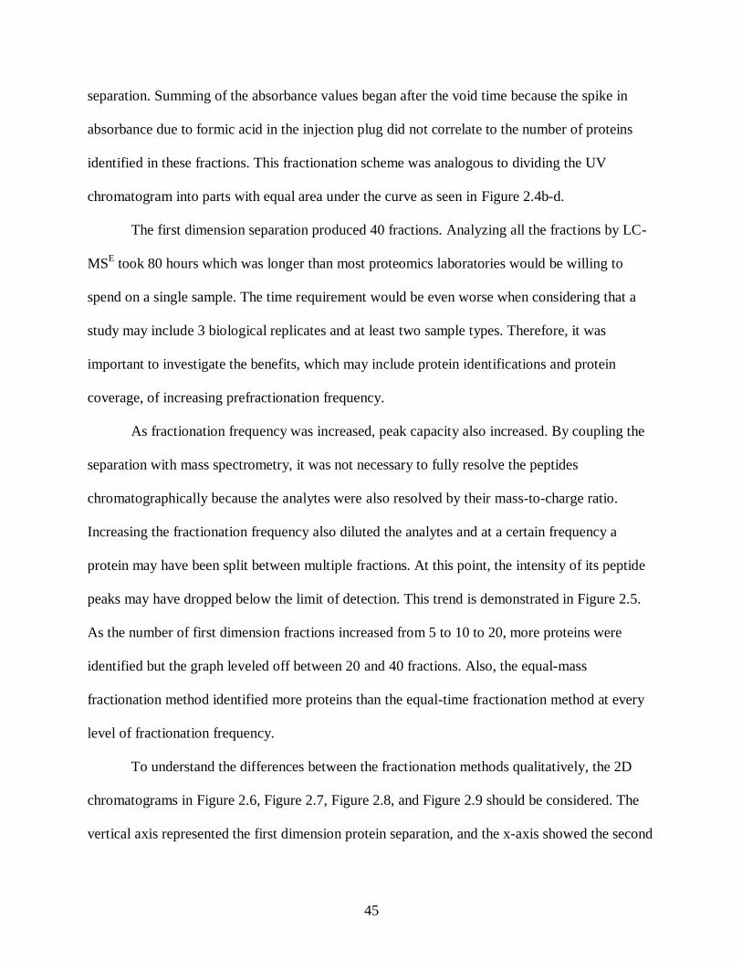
45
separation. Summing of the absorbance values began after the void time because the spike in
absorbance due to formic acid in the injection plug did not correlate to the number of proteins
identified in these fractions. This fractionation scheme was analogous to dividing the UV
chromatogram into parts with equal area under the curve as seen in Figure 2.4b-d.
The first dimension separation produced 40 fractions. Analyzing all the fractions by LC-
MSE took 80 hours which was longer than most proteomics laboratories would be willing to
spend on a single sample. The time requirement would be even worse when considering that a
study may include 3 biological replicates and at least two sample types. Therefore, it was
important to investigate the benefits, which may include protein identifications and protein
coverage, of increasing prefractionation frequency.
As fractionation frequency was increased, peak capacity also increased. By coupling the
separation with mass spectrometry, it was not necessary to fully resolve the peptides
chromatographically because the analytes were also resolved by their mass-to-charge ratio.
Increasing the fractionation frequency also diluted the analytes and at a certain frequency a
protein may have been split between multiple fractions. At this point, the intensity of its peptide
peaks may have dropped below the limit of detection. This trend is demonstrated in Figure 2.5.
As the number of first dimension fractions increased from 5 to 10 to 20, more proteins were
identified but the graph leveled off between 20 and 40 fractions. Also, the equal-mass
fractionation method identified more proteins than the equal-time fractionation method at every
level of fractionation frequency.
To understand the differences between the fractionation methods qualitatively, the 2D
chromatograms in Figure 2.6, Figure 2.7, Figure 2.8, and Figure 2.9 should be considered. The
vertical axis represented the first dimension protein separation, and the x-axis showed the second

46
dimension peptide separation. The peak height was represented by false color in the z-direction.
For the chromatograms of the equal-time fractions, the number of peaks decreased towards the
end of the chromatogram. This corresponds to fractions 30-40 in Figure 2.6, 16-20 in Figure
2.7a, 8-10 in Figure 2.8a, and fraction 5 in Figure 2.9a. In fact, the same trypsin autolysis peaks
dominated the chromatograms of these fractions. In comparison, the equal-mass chromatograms
appeared to have unique bands for each fraction.
2.3.2 Proteins per fraction
To confirm that more proteins were identified in the late eluting fractions of the equal-
mass method, the number of protein identifications was plotted for each fraction in the bar
graphs in Figure 2.10, Figure 2.11, Figure 2.12, and Figure 2.13. The light gray bars showed the
total number of proteins identifications in each fraction, and the dark gray bars signified the
number of unique proteins found in each fraction. Proteins found in multiple fractions were
assigned to the fraction in which it was most intense. The first eluting fractions, corresponding to
the injection plug, contained few protein identifications. A couple of factors may have
contributed to the low number of identifications. (1) There were no proteins eluting in the
injection plug. (2) The injection plug contains large proteins or agglomerated proteins that were
excluded from the stationary phase. Large proteins were often difficult to digest because they did
not fully denature blocking trypsin from the digestion sites. The total number of proteins
identified in the late eluting fractions remained relatively constant for both the equal-time and
equal-mass fractionation methods. However, the number of unique protein identifications in the
late eluting fractions was greater for the equal-mass than the equal-time fractionation method.
For the equal-mass fractions, the number of unique protein identifications was more even
fraction to fraction. With the instrumentation used for this experiment, it seemed that a limited

47
maximum number of proteins could be identified per fraction. By more evenly distributing the
proteins between the fractions, as achieved with the equal-mass fractionation method, the
number of unique protein identifications increased. Figure 2.5 showed a 19% increase in
identifications for 5 fractions, 22% for 10 fractions, and 10% for 20 fractions.
2.3.3 Venn comparison
The Venn diagram of proteins identifications in Figure 2.14a showed that most of the
proteins identified in the 5 equal-time fractions were also identified in the 10 equal-time
fractions. Additionally, 103 new proteins were identified with only 9 identifications lost which
yielded an improvement of 40%. Similarly, when equal-time fractionation was increased to 20,
175 more identifications were made with only a loss of 8 identifications which was also a gain of
40%. A similar trend was observed for the equal-mass fractions in Figure 2.15. However, the
Venn diagram in Figure 2.14b showed that while 78 new proteins were identified in the 40
equal-time fractions, 41 were lost. In doubling the analysis time, protein identifications were
only improved by 9%. It was hypothesized that the loss of 41 protein identifications was due to
proteins being split between multiple fractions.
2.3.4 Fractions per protein
Ideally, a protein peak should not be split between multiple fractions. The probability of
peak splitting increases as fractionation frequency increases. Also, a protein may have appeared
in multiple fractions due to different post translational modifications and variations in its tertiary
structure. To determine the amount of peak splitting between multiple first dimension fractions,
the percentage of protein identifications that were identified in only one fraction, two fractions,
and three-or-more fractions were plotted in Figure 2.16. For every fractionation scheme, the
majority of the proteins were identified in only one fraction. The highest percentage of proteins

48
being identified in only one fraction occurred when only 5 first dimension fractions were taken.
This percentage decreased as fractionation frequency increased. The percentage of proteins
identified in multiple fractions was similar for the 5 and 10 first dimension fraction sets. A nearly
50% increase of proteins found in multiple fractions was observed when prefractionation was
increased to 20 and 40 fractions. When considering the equal-mass fractionation method, a larger
portion of proteins was identified in only one fraction as compared to the equal-time
fractionation method. For example, 80% of the proteins were identified in only one fraction in
the 5 equal-mass fractionation set, and 70% of proteins were identified in only one fraction in the
5 equal-time fractionation set. A larger percentage of proteins were identified in 3 or more
fractions by the equal-time than the equal-mass fractionation method.
2.3.5 Normalized Difference Protein Coverage
When discussing the merit of multidimensional proteomic separations, it was not merely
enough to report the total number of proteins identifications without further commenting on
protein coverage. To compare the methods, coverage is reported in Table 2.3. for several proteins
involved in the metabolic processes of yeast. On average, coverage increased with higher
fractionation frequency. For a large data set containing hundreds of proteins, comparing the
coverage for each protein is not straight forward. For example, reducing protein coverage to an
average can be misleading. The additional proteins identified in a separation with higher peak
capacity were usually of lower abundance and had lower coverage, bringing down the average.
Alternatively, comparing only proteins identified by both methods would limit the analysis to
only easily detectible proteins which usually had higher coverage and, thus, mute the difference
between the methods. Herein, an original method to compare protein coverage based on the
mathematical concept of a normalized difference is described. We named this metric the
49
normalized difference protein coverage (NDPC) and define it as the difference in coverage of a
protein between two methods divided by the sum of the coverage. The NDPC was calculated as
follows:
NDPC Coveragea,i- Coveragea,
Coveragea,i Coveragea, , (2-4)
where was the percent coverage of protein a in method i, and
was the percent coverage of protein a in method j. For example, the NDPC for fumarate
hydratase (FUMH), a protein involved in the citric acid cycle of S. cerevisiae, was calculated to
compare 10 equal-time and 10 equal-mass fractions:
NDPC Coverage
FUMH,1 equal-mass- Coverage
FUMH,1 equal-time
CoverageFUMH,1 equal-mass
CoverageFUMH,1 equal-time
, (2-5)
52-36
52 36 .1 (2-6)
With this example, a protein found with higher coverage in the 10 equal-mass fractions
would have a positive NDPC. A negative NDPC would signify that the protein was found with
higher coverage in the 10 equal-time fractions. A value of +1 meant the protein was only
identified in the 10 equal-mass fractions, and a value of -1 meant the protein was only identified
in the 10 equal-time fractions. The equal-time and equal-mass prefractionation methods were
compared for 5 fractions in Figure 2.17, for 10 fractions in Appendix A.1. and for 20 fractions in
Appendix A.2. The NDPC values were plotted with the proteins ordered from largest to smallest
denominator, putting the proteins with highest coverage on the left, and the lowest coverage on
the right. The absolute values of NDPC increased as the denominator (summed protein coverage)
decreased. These figures were large and split amongst several pages. To better comprehend the
trend, the protein identifier information was removed so the graph could fit onto a single page.
The abundance of red lines in Figure 2.18.a. and Figure 2.18.b. signified higher coverage in the 5
50
and 10 equal-mass fractions. When fractionation increased to 20 (Figure 2.18.c.), there was little
difference in coverage between the two methods.
In an attempt to further simplify the comparison of coverage between multiple methods,
while maintaining the meaning of the values, we propose the Grand NDPC which is calculated
by the difference between the grand total protein coverage in method one and method two
normalized by the grand sum of protein coverage in both methods. An example calculation is
shown in Equation 2-5:
rand NDPC (∑Coverage
method 1) - (∑Coverage
method 2)
∑Coveragemethod 1
∑Coveragemethod 2
(2-7)
Perhaps a more relevant interpretative of the Grand NDPC would be to relate it to a fold-
change improvement in coverage as follows:
Fold-Change in Coverage ∑Coverage
method 1
∑Coveragemethod 2
1 rand NDPC
1- rand NDPC (2-8)
If the fold-change was less than one, the negative reciprocal of the value was used as is
conventional with fold-change calculations. The Grand NDPC and Fold-Change in Coverage is
listed in Table 2.4 for each fractionation frequency. Positive values represented higher coverage
with the equal-mass fractionation method, and negative values represented higher coverage with
the equal-time fractionation method. The Grand NDPC and Fold-Change Coverage increased in
favor of the equal-mass method for 5 and 10 fractions. The largest fold-change improvement was
1.4 with the 10 fraction comparison. No significant difference in coverage was observed between
the two methods with 20 first dimension fractions.
2.4 Conclusion
While this was a limited study of only one organism, it can serve as a guide for
multidimensional method development with prefractionation. Protein identifications increased as

51
fractionation frequency was increased. These benefits had diminishing returns with respect to
time as prefractionation increased to more than 20 fractions. The equal-mass prefractionation
method proved to be a good technique to get more information out of a sample in the same
amount of time as compared to the equal-time fractionation method. Future improvements could
be made to the second dimension separation. The use of a LC with higher pressure limitations
could make possible the use of smaller particles and longer columns to improve peak capacity
without increasing analysis time.

52
2.5 TABLES
Time
(min)
Flow Rate
(mL/min)
90:5:5
H2O:ACN:IPA +
0.2% TFA
(%A)
50:50
ACN:IPA
+ 0.2% TFA
(%B)
0 1.0 100 0
2 1.0 100 0
5 1.0 75 25
40 1.0 50 50
45 1.0 35 65
45.1 1.0 0 100
50 1.0 0 100
50.1 1.0 100 0
Table 2.1. Chromatographic conditions for the reversed-phase prefractionation of intact proteins.

53
Integrated TIC of 40 Fractions
Fraction Rep 1 (x107) Rep 2 (x107) Rep 3 (x107) Average Summed Normalized
1 0.38 0.31 0.20 0.30 0.30 0.00
2 0.64 0.32 0.21 0.39 0.68 0.01
3 1.93 0.96 1.15 1.35 2.03 0.02
4 2.22 1.26 1.29 1.59 3.62 0.03
5 1.92 2.03 1.40 1.78 5.40 0.05
6 4.59 4.56 3.07 4.07 9.48 0.09
7 6.31 3.94 4.11 4.78 14.26 0.13
8 6.20 5.32 4.32 5.28 19.54 0.18
9 3.42 3.42 2.48 3.11 22.65 0.20
10 2.98 2.18 2.02 2.40 25.04 0.23
11 2.96 2.37 1.98 2.43 27.48 0.25
12 2.97 2.26 1.85 2.36 29.84 0.27
13 4.14 3.19 2.22 3.18 33.02 0.30
14 3.43 2.65 2.21 2.76 35.78 0.32
15 4.73 4.25 3.12 4.03 39.81 0.36
16 6.01 5.86 3.66 5.18 44.99 0.41
17 9.41 8.76 5.37 7.85 52.84 0.48
18 6.23 6.27 3.89 5.46 58.30 0.53
19 8.47 6.16 5.01 6.55 64.84 0.59
20 8.64 6.01 4.82 6.49 71.34 0.64
21 8.14 4.85 3.92 5.64 76.97 0.69
22 9.03 5.65 4.64 6.44 83.41 0.75
23 5.82 3.00 2.59 3.80 87.22 0.79
24 5.94 2.67 3.01 3.87 91.09 0.82
25 6.32 5.01 3.92 5.09 96.18 0.87
26 3.27 2.26 2.26 2.60 98.77 0.89
27 2.95 1.84 2.02 2.27 101.04 0.91
28 1.99 1.22 1.44 1.55 102.59 0.93
29 2.22 0.95 1.39 1.52 104.11 0.94
30 0.21 0.82 1.10 0.71 104.82 0.95
31 1.16 0.53 0.78 0.83 105.65 0.95
32 1.05 0.48 0.76 0.76 106.41 0.96
33 0.54 0.25 0.44 0.41 106.82 0.96
34 1.02 0.41 0.55 0.66 107.48 0.97
35 0.89 0.37 0.54 0.60 108.08 0.98
36 0.80 0.28 0.50 0.53 108.61 0.98
37 0.91 0.37 0.64 0.64 109.25 0.99
38 0.81 0.26 0.61 0.56 109.81 0.99
39 0.60 0.22 0.52 0.44 110.26 1.00
40 0.65 0.26 0.63 0.52 110.77 1.00
Table 2.2. Integrated TIC values, summed integrated TIC, and normalized summed integrated
TIC value used to determine first dimension fractionation schemes.

54
Protein Coverage (%)
Number of equal-time fractions
Number of equal-mass fractions
Name Accession
5 10 20 40
5 10 20
6-phosphogluconate dehydrogenase 6PGD1
61% 39% 76% 70%
29% 54% 63%
Isocitrate lyase ACEA
- - 29% 38%
3% 31% 41%
Aconitate hydratase, mito ACON
38% 46% 47% 49%
44% 48% 40%
Acetyl-coenzyme A synthetase 1 ACS1
25% 30% 51% 49%
24% 42% 55%
Alcohol dehydrogenase 1 ADH1
60% 58% 65% 69%
62% 69% 59%
Alcohol dehydrogenase 2 ADH2
66% 72% 71% 73%
69% 73% 67%
Alcohol dehydrogenase 3, mito ADH3
8% - 19% 17%
- 22% 18%
Alcohol dehydrogenase 6 ADH6
- - 3% -
- - -
K-activated aldehyde dehydrogenase ALDH4
75% 72% 81% 88%
75% 87% 83%
Aldehyde dehydrogenase 5, mito ALDH5
- - - -
- - -
Fructose-bisphosphate aldolase ALF
69% 76% 69% 81%
73% 71% 75%
Citrate synthase, mito CISY1
31% 35% 52% 57%
45% 53% 61%
Dihydrolipoyl dehydrogenase, mito DLDH
39% 38% 77% 70%
32% 39% 72%
Enolase 1 ENO1
73% 80% 79% 83%
76% 84% 81%
Enolase 2 ENO2
76% 78% 86% 87%
83% 81% 87%
Fumarate reductase FRDS
- 8% 21% 24%
6% 22% 25%
Fumarate hydratase, mitoc FUMH
26% 36% 43% 53%
27% 52% 49%
Glyceraldehyde-3-P dehydrogenase 1 G3P1
71% 70% 85% 77%
74% 79% 76%
Glyceraldehyde-3-P dehydrogenase 2 G3P2
83% 71% 89% 87%
83% 84% 88%
Glyceraldehyde-3-P dehydrogenase 3 G3P3
90% 78% 92% 90%
91% 92% 91%
Glucose-6-phosphate isomerase G6PI
61% 60% 69% 60%
52% 64% 65%
Hexokinase-1 HXKA
52% 56% 80% 75%
50% 68% 76%
Hexokinase-2 HXKB
60% 53% 84% 74%
61% 67% 69%
Glucokinase-1 HXKG
54% 40% 69% 68%
57% 72% 67%
6-phosphofructokinase subunit α K6PF1
8% 8% 32% 28%
24% 31% 24%
Pyruvate kinase 1 KPYK1
59% 68% 85% 81%
76% 83% 81%
Malate dehydrogenase, cyto MDHC
26% 35% 64% 44%
22% 39% 52%

55
Protein Coverage (%)
Number of equal-time fractions
Number of equal-mass fractions
Name Accession
5 10 20 40
5 10 20
Malate dehydrogenase, mito MDHM
75% 78% 74% 76%
68% 82% 76%
Pyruvate dehydrogenase E1 comp β ODPB
- - 17% 29%
- 9% 33%
Phosphoenolpyruvate carboxykinase PCKA
41% 53% 59% 61%
46% 57% 59%
Pyruvate decarboxylase isozyme 1 PDC1
63% 65% 74% 74%
55% 68% 67%
Phosphoglycerate kinase PGK
79% 70% 84% 86%
83% 88% 84%
Phosphoglycerate mutase 1 PMG1
76% 79% 76% 69%
78% 76% 54%
Pyruvate carboxylase 1 PYC1
- - 18% 38%
- 4% 38%
Succinyl-CoA ligase subunit α SUCA
60% 67% 84% 71%
60% 72% 69%
Succinyl-CoA ligase subunit β SUCB
- 16% 38% 37%
13% 38% 30%
Transketolase 1 TKT1
15% 22% 43% 51%
27% 54% 49%
Transketolase 2 TKT2
- - 6% 20%
- 14% 21%
Triosephosphate isomerase TPIS
76% 75% 82% 89%
80% 88% 86%
Average
55% 54% 60% 62%
53% 58% 60%
Table 2.3. The protein coverage (%) was reported for some of the proteins involved in S. cerevisiae metabolism. Generally, protein
coverage increased with fractionation frequency.

56
Number of Fractions Grand NDPC Fold-Change in Coverage
5 0.050 1.1
10 0.17 1.4 20 -0.0093 -1.0
Table 2.4. The Grand NDPC and Fold-Change in Coverage was listed in for each fractionation
frequency. Positive values represented higher coverage with the equal-mass fractionation
method, and negative values represented higher coverage with the equal-time fractionation
method. The Grand NDPC and Fold-Change in Coverage favored of the equal-mass method for
5 and 10. The largest fold-change improvement was 1.4 with the 10 fraction comparison. No
significant difference in coverage was observed between the two methods with 20 first
dimension fractions.
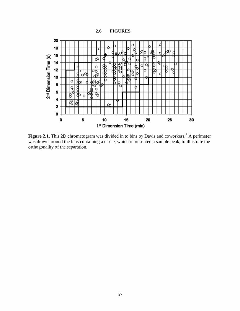
57
2.6 FIGURES
Figure 2.1. This 2D chromatogram was divided in to bins by Davis and coworkers.7 A perimeter
was drawn around the bins containing a circle, which represented a sample peak, to illustrate the
orthogonality of the separation.
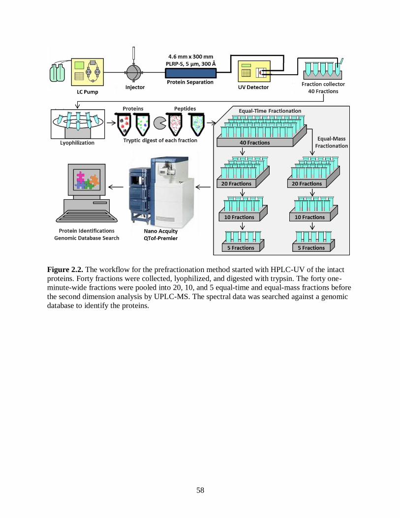
58
Figure 2.2. The workflow for the prefractionation method started with HPLC-UV of the intact
proteins. Forty fractions were collected, lyophilized, and digested with trypsin. The forty one-
minute-wide fractions were pooled into 20, 10, and 5 equal-time and equal-mass fractions before
the second dimension analysis by UPLC-MS. The spectral data was searched against a genomic
database to identify the proteins.

59
Figure 2.3. The representative TIC chromatogram from a peptide (second dimension) separation
of the 40 equal-time fraction set showed an example of peak integration. The peak area was the
∫TIC value used in Table 2.2 for the determination of the equal-mass prefractionation schemes.
7x10⁵
6
5
4
3
2
1
0
To
tal
Ion
Cu
rren
t (T
IC)
10080604020
Time (min)
TIC
Fraction 9 of 40
3.42 x 10⁷ Counts
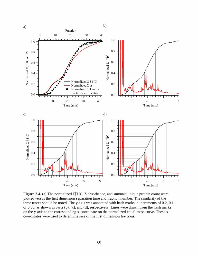
60
a)
b)
c)
d)
Figure 2.4. (a) The normalized Σ∫TIC, Σ absorbance, and summed unique protein count were
plotted versus the first dimension separation time and fraction number. The similarity of the
three traces should be noted. The y-axis was annotated with hash marks in increments of 0.2, 0.1,
or 0.05, as shown in parts (b), (c), and (d), respectively. Lines were drawn from the hash marks
on the y-axis to the corresponding x-coordinate on the normalized equal-mass curve. These x-
coordinates were used to determine size of the first dimension fractions.
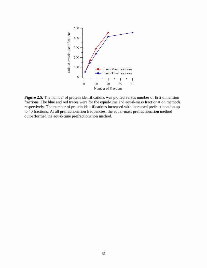
61
Figure 2.5. The number of protein identifications was plotted versus number of first dimension
fractions. The blue and red traces were for the equal-time and equal-mass fractionation methods,
respectively. The number of protein identifications increased with increased prefractionation up
to 40 fractions. At all prefractionation frequencies, the equal-mass prefractionation method
outperformed the equal-time prefractionation method.

62
Figure 2.6. The 2D chromatogram for 40 first dimension fractions was plotted with the first
dimension (protein) separation time and fraction number plotted on the vertical axes and the
second dimension (peptide) separation on the bottom axis. Starting with fraction 30, the peak
pattern repeated for all subsequent fractions. These peaks corresponded to peptides from trypsin
autolysis.

63
a) Equal-Time Fractions
b) Equal-Mass Fractions
Figure 2.7. The 2D chromatograms for 20 first dimension fractions were plotted with the first dimension (protein) separation time or
fraction number plotted on the vertical axes and the second dimension (peptide) separation on the bottom axis. Peak intensity was
plotted in the z-direction. In the later eluting fractions, more peaks were observed in (b) the equal-mass fractionation chromatogram
than in (a) the equal-time fractionation chromatogram.
20
18
16
14
12
10
8
6
4
2
Fractio
n n
um
ber
10080604020Reveresed phase retention time (min)
40
36
32
28
24
20
16
12
8
4
Rev
erse
d p
has
e re
ten
tio
n t
ime
(min
)
Peptide Separation
Pro
tein
Sep
arat
ion
10080604020Reversed phase retention time (min)
20
18
16
14
12
10
8
6
4
2
0
Rev
erse
d p
has
e fr
acti
on
Peptide Separation
Pro
tein
Sep
arat
ion

64
a) Equal-Time Fractions
b) Equal-Mass Fractions
Figure 2.8. The 2D chromatograms for 10 first dimension fractions were plotted with the first dimension (protein) separation time or
fraction number plotted on the vertical axes and the second dimension (peptide) separation on the bottom axis. Peak intensity was
plotted in the z-direction. In the later eluting fractions, more peaks were observed in (b) the equal-mass fractionation chromatogram
than in (a) the equal-time fractionation chromatogram.
10
9
8
7
6
5
4
3
2
1
Fractio
n n
um
ber
10080604020Reversed phase retention time (min)
40
36
32
28
24
20
16
12
8
4
Rev
erse
d p
has
e re
ten
tio
n t
ime
(min
)P
rote
in S
epar
atio
n
Peptide Separation
100755025Reversed phase retention time (min)
10
9
8
7
6
5
4
3
2
1
0
Rev
erse
d p
has
e re
ten
tio
n t
ime
(min
)
Peptide Separation
Pro
tein
Sep
arat
ion

65
a) Equal-Time Fractions
b) Equal-Mass Fractions
Figure 2.9. The 2D chromatograms for 5 first dimension fractions were plotted with the first dimension (protein) separation time or
fraction number plotted on the vertical axes and the second dimension (peptide) separation on the bottom axis. Peak intensity was
plotted in the z-direction. In the later eluting fractions, more peaks were observed in (b) the equal-mass fractionation chromatogram
than in (a) the equal-time fractionation chromatogram.
5
4
3
2
1
Fractio
n n
um
ber
10080604020Reversed phase retention time (min)
40
36
32
28
24
20
16
12
8
4
Rev
erse
d p
has
e re
ten
tio
n t
ime
(min
)
Peptide Separation
Pro
tein
Sep
arat
ion
10080604020Reversed phase retention time (min)
5
4
3
2
1
0
Rev
erse
d p
has
e fr
acti
on
Peptide Separation
Pro
tein
Sep
arat
ion

66
Figure 2.10. The light gray bars show the total protein identifications in each fraction, and the
dark gray bars signify the unique protein identifications in each fraction for 40 first dimensional
fractions. The number of unique protein identifications decreased in the last 15 fractions faster
than the total protein identifications. This trend was less pronounced as prefractionation
frequency decreased.

67
a)
b)
Figure 2.11. The light gray bars show the total protein identifications in each fraction, and the
dark gray bars signify the unique protein identifications in each fraction for 20 first dimensional
fractions. By more evenly distributing the sample mass between the fractions, as with the equal-
mass fractionation method (b), the number of unique protein identifications was more even
fraction to fraction and increased in the late eluting fractions as compared to the equal-time
fractionation method (a).

68
a)
b)
Figure 2.12. The light gray bars show the total protein identifications in each fraction, and the
dark gray bars signify the unique protein identifications in each fraction for 10 first dimensional
fractions. By more evenly distributing the sample mass between the fractions, as with the equal-
mass fractionation method (b), the number of unique protein identifications was more even
fraction to fraction and increased in the late eluting fractions as compared to the equal-time
fractionation method (a).

69
a)
b)
Figure 2.13. The light gray bars show the total protein identifications in each fraction, and the
dark gray bars signify the unique protein identifications in each fraction for 5 first dimensional
fractions. By more evenly distributing the sample mass between the fractions, as with the equal-
mass fractionation method (b), the number of unique protein identifications was more even
fraction to fraction and increased in the late eluting fractions as compared to the equal-time
fractionation method (a).

70
a)
b)
Figure 2.14. Venn diagram (a) showed the overlap in protein identifications for 5, 10, and 20 equal-time fractions. Increasing
fractionation to 20 led to new protein identifications while still identifying most of the proteins identified in the five and ten fraction
sets. Venn diagram (b) showed the overlap in protein identifications for 20 and 40 equal-time fractions.
135
1
6
1 5
8
1 Fractions
238
2 Fractions
414
5 Fractions
144
5 33 116
2 Fractions
414
4 Fractions
455

71
Figure 2.15. The Venn diagram showed the overlap in protein identifications for 5, 10, and 20
equal-mass fractions. Increasing fractionation to 20 led to new protein identifications while still
identifying most of the proteins identified in the five and ten fraction sets.
212
1
2
14
22
163
6
1 Fractions
3 6
2 Fractions
521
5 Fractions
221

72
Figure 2.16. Fractions per protein described the percentage of protein identifications that were detected in one, two, or more fractions
(3+). As prefractionation frequency increased, more proteins were identified in multiple fractions. This effect was heightened for the
equal-time fractions (blue) as compared to the equal-mass fractions (red).

73
Figure 2.17. To compare the 5 equal-mass and 5 equal-time fractions, the Normalized
Difference Protein Coverage (NDPC) was plotted with proteins with higher coverage on the left,
and proteins with lower coverage on the right. If a protein was identified with higher sequence
coverage in the 5 equal-mass fractions, its NDPC value was positive (red bars). The blue bars
signified higher coverage in the 5 equal-time fractions. Differences in coverage were minimal for
highly covered proteins. As protein coverage decreased, more proteins were identified with
higher coverage in the equal-mass fractions. The dashed lines indicate a level of two-fold greater
protein coverage.

74
Figure 2.17. (continued)

75
Figure 2.17. (continued)

76
a)
b)
c)
Figure 2.18. The NDPC compared the equal-mass and equal-time methods for 5 (part a), 10
(part b), and 20 (part c) first dimension fractions. If a protein was identified with higher sequence
coverage in the equal-mass fractions, the NDPC value was positive (red lines). The blue lines
signified higher coverage in the equal-time fractions. Proteins with higher coverage were plotted
on the left, and proteins with lower coverage were on the right. Differences in coverage were
minimal for highly covered proteins. As protein coverage decreased, more proteins were
identified with higher coverage by the equal-mass method for 5 and 10 fractions. There was little
difference in NDPC for 20 equal-mass and 20 equal-time fractions.

77
2.7 REFERENCES
1. Xie, F.; Smith, R. D.; Shen, Y., Advanced proteomic liquid chromatography. Journal of
Chromatography A 2012, 1261 (0), 78-90.
2. Wolters, D. A.; Washburn, M. P.; Yates, J. R., An Automated Multidimensional Protein
Identification Technology for Shotgun Proteomics. Analytical Chemistry 2001, 73 (23),
5683-5690.
3. Washburn, M. P.; Ulaszek, R.; Deciu, C.; Schieltz, D. M.; Yates, J. R., Analysis of
Quantitative Proteomic Data Generated via Multidimensional Protein Identification
Technology. Analytical Chemistry 2002, 74 (7), 1650-1657.
4. Giddings, J. C., Unified separation science. Wiley: 1991.
5. Rutan, S. C.; Davis, J. M.; Carr, P. W., Fractional coverage metrics based on ecological
home range for calculation of the effective peak capacity in comprehensive two-
dimensional separations. Journal of Chromatography A 2012, 1255 (0), 267-276.
6. Gu, H.; Huang, Y.; Carr, P. W., Peak capacity optimization in comprehensive two
dimensional liquid chromatography: A practical approach. Journal of Chromatography A
2011, 1218 (1), 64-73.
7. Davis, J. M.; Stoll, D. R.; Carr, P. W., Dependence of Effective Peak Capacity in
Comprehensive Two-Dimensional Separations on the Distribution of Peak Capacity
between the Two Dimensions. Analytical Chemistry 2008, 80 (21), 8122-8134.
8. Gilar, M.; Olivova, P.; Daly, A. E.; Gebler, J. C., Orthogonality of Separation in Two-
Dimensional Liquid Chromatography. Analytical Chemistry 2005, 77 (19), 6426-6434.
9. Siegler, W. C.; Fitz, B. D.; Hoggard, J. C.; Synovec, R. E., Experimental Study of the
Quantitative Precision for Valve-Based Comprehensive Two-Dimensional Gas
Chromatography. Analytical Chemistry 2011, 83 (13), 5190-5196.
10. Sheldon, E. M., Development of a LC–LC–MS complete heart-cut approach for the
characterization of pharmaceutical compounds using standard instrumentation. Journal of
Pharmaceutical and Biomedical Analysis 2003, 31 (6), 1153-1166.
11. Schure, M. R., Limit of Detection, Dilution Factors, and Technique Compatibility in
Multidimensional Separations Utilizing Chromatography, Capillary Electrophoresis, and
Field-Flow Fractionation. Analytical Chemistry 1999, 71 (8), 1645-1657.
12. Gilar, M.; Daly, A. E.; Kele, M.; Neue, U. D.; Gebler, J. C., Implications of column peak
capacity on the separation of complex peptide mixtures in single- and two-dimensional
high-performance liquid chromatography. Journal of Chromatography A 2004, 1061 (2),
183-192.
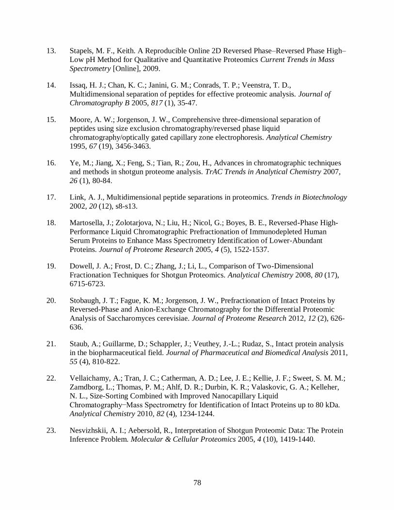
78
13. Stapels, M. F., Keith. A Reproducible Online 2D Reversed Phase–Reversed Phase High–
Low pH Method for Qualitative and Quantitative Proteomics Current Trends in Mass
Spectrometry [Online], 2009.
14. Issaq, H. J.; Chan, K. C.; Janini, G. M.; Conrads, T. P.; Veenstra, T. D.,
Multidimensional separation of peptides for effective proteomic analysis. Journal of
Chromatography B 2005, 817 (1), 35-47.
15. Moore, A. W.; Jorgenson, J. W., Comprehensive three-dimensional separation of
peptides using size exclusion chromatography/reversed phase liquid
chromatography/optically gated capillary zone electrophoresis. Analytical Chemistry
1995, 67 (19), 3456-3463.
16. Ye, M.; Jiang, X.; Feng, S.; Tian, R.; Zou, H., Advances in chromatographic techniques
and methods in shotgun proteome analysis. TrAC Trends in Analytical Chemistry 2007,
26 (1), 80-84.
17. Link, A. J., Multidimensional peptide separations in proteomics. Trends in Biotechnology
2002, 20 (12), s8-s13.
18. Martosella, J.; Zolotarjova, N.; Liu, H.; Nicol, G.; Boyes, B. E., Reversed-Phase High-
Performance Liquid Chromatographic Prefractionation of Immunodepleted Human
Serum Proteins to Enhance Mass Spectrometry Identification of Lower-Abundant
Proteins. Journal of Proteome Research 2005, 4 (5), 1522-1537.
19. Dowell, J. A.; Frost, D. C.; Zhang, J.; Li, L., Comparison of Two-Dimensional
Fractionation Techniques for Shotgun Proteomics. Analytical Chemistry 2008, 80 (17),
6715-6723.
20. Stobaugh, J. T.; Fague, K. M.; Jorgenson, J. W., Prefractionation of Intact Proteins by
Reversed-Phase and Anion-Exchange Chromatography for the Differential Proteomic
Analysis of Saccharomyces cerevisiae. Journal of Proteome Research 2012, 12 (2), 626-
636.
21. Staub, A.; Guillarme, D.; Schappler, J.; Veuthey, J.-L.; Rudaz, S., Intact protein analysis
in the biopharmaceutical field. Journal of Pharmaceutical and Biomedical Analysis 2011,
55 (4), 810-822.
22. Vellaichamy, A.; Tran, J. C.; Catherman, A. D.; Lee, J. E.; Kellie, J. F.; Sweet, S. M. M.;
Zamdborg, L.; Thomas, P. M.; Ahlf, D. R.; Durbin, K. R.; Valaskovic, G. A.; Kelleher,
N. L., Size-Sorting Combined with Improved Nanocapillary Liquid
Chromatography−Mass Spectrometry for Identification of Intact Proteins up to 80 kDa.
Analytical Chemistry 2010, 82 (4), 1234-1244.
23. Nesvizhskii, A. I.; Aebersold, R., Interpretation of Shotgun Proteomic Data: The Protein
Inference Problem. Molecular & Cellular Proteomics 2005, 4 (10), 1419-1440.
79
24. Bigelow, C. C., On the average hydrophobicity of proteins and the relation between it and
protein structure. Journal of Theoretical Biology 1967, 16 (2), 187-211.
25. McCoy, B. J., Multidimensional chromatography—techniques and applications. Edited
by H. J. Cortes, Marcel Dekker, New York, NY, 1990, 424 pp. $99.75 (U.S. and
Canada), $119.50 (all other countries). AIChE Journal 1990, 36 (12), 1933-1933.
26. Bradford, M. M., A rapid and sensitive method for the quantitation of microgram
quantities of protein utilizing the principle of protein-dye binding. Analytical
Biochemistry 1976, 72 (1–2), 248-254.
27. Searle, B. C., Scaffold: A bioinformatic tool for validating MS/MS-based proteomic
studies. PROTEOMICS 2010, 10 (6), 1265-1269.
28. Eng, J. K.; Searle, B. C.; Clauser, K. R.; Tabb, D. L., A Face in the Crowd: Recognizing
Peptides Through Database Search. Molecular & Cellular Proteomics 2011, 10 (11).

80
CHAPTER 3. Increasing Peak Capacities for Peptide Separations Using Long
Microcapillary Columns and Sub-2 μm Particles at 30,000+ psi
3.1 Introduction
The field of proteomics is growing in popularity as understanding protein expression in
biological systems is essential to elucidating the mechanism of diseases.1 Analysis of proteins is
complicated because there are thousands of proteins in a cell spanning a large range of
abundances (greater than 1010
).2 To reduce the complexity, many proteomic experiments include
a separation by reversed phase liquid chromatography (RPLC) before introduction into the mass
spectrometer.3 Because protein separations are plagued by sample carryover, and the ionization
and fragmentation efficiency of proteins are low, many experiments start with a digestion before
the separation which increases the number of components in the mixture.4,5,6,7
3.1.1 Coupling LC with MS
To date, no single-dimension separation technique exists with the peak capacity to
completely resolve an entire proteome.8 This issue has been mitigated by the coupling of LC to
MS which can detect many species in a single scan. Efforts have been made in the field of mass
spectrometry to increase acquisition rates while simultaneously improving limits of detection.
The invention of nanoESI resulted in higher ionization efficiency, reduced matrix effects, and
facilitated the coupling of LC to MS.9,10,11,12
Incorporating ion mobility into the mass
spectrometer adds another level of analyte separation based on drift time without increasing total
analysis time.13
To handle the massive amounts of information acquired during proteomic
experiments, bioinformaticians have developed several programs to mine the data for
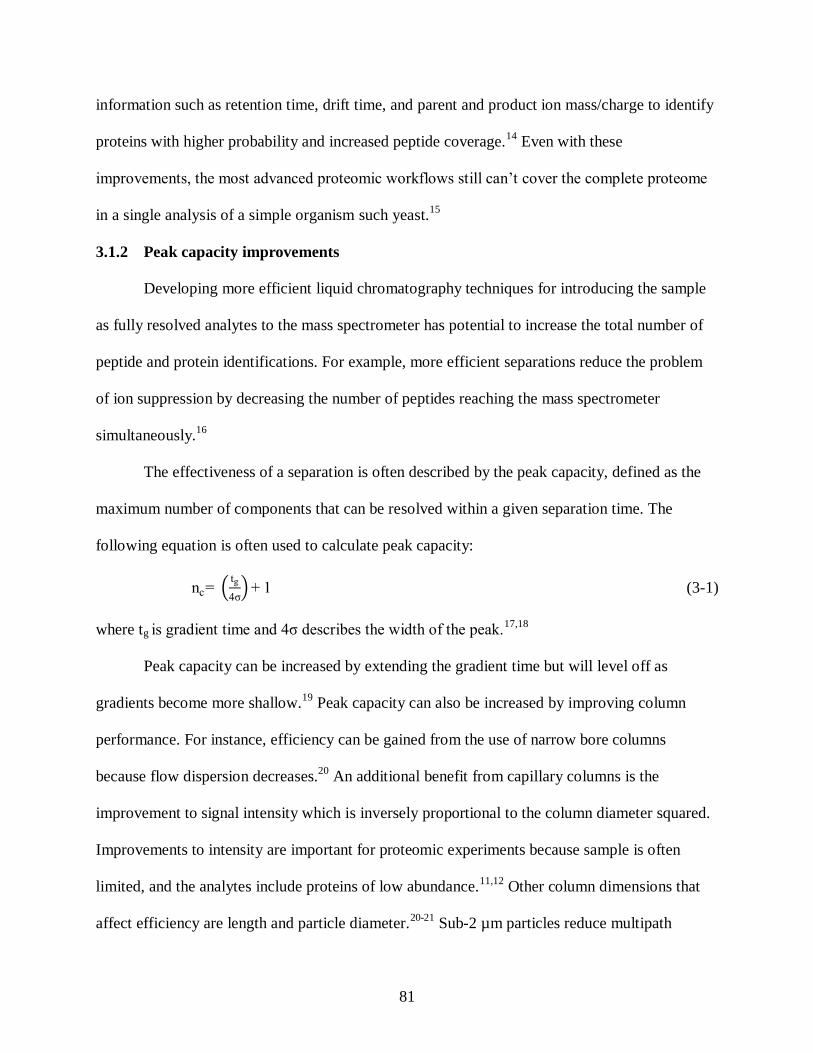
81
information such as retention time, drift time, and parent and product ion mass/charge to identify
proteins with higher probability and increased peptide coverage.14
Even with these
improvements, the most advanced proteomic workflows still can’t cover the complete proteome
in a single analysis of a simple organism such yeast.15
3.1.2 Peak capacity improvements
Developing more efficient liquid chromatography techniques for introducing the sample
as fully resolved analytes to the mass spectrometer has potential to increase the total number of
peptide and protein identifications. For example, more efficient separations reduce the problem
of ion suppression by decreasing the number of peptides reaching the mass spectrometer
simultaneously.16
The effectiveness of a separation is often described by the peak capacity, defined as the
maximum number of components that can be resolved within a given separation time. The
following equation is often used to calculate peak capacity:
nc (tg
4σ) 1 (3-1)
where tg is gradient time and 4σ describes the width of the peak.17,18
Peak capacity can be increased by extending the gradient time but will level off as
gradients become more shallow.19
Peak capacity can also be increased by improving column
performance. For instance, efficiency can be gained from the use of narrow bore columns
because flow dispersion decreases.20
An additional benefit from capillary columns is the
improvement to signal intensity which is inversely proportional to the column diameter squared.
Improvements to intensity are important for proteomic experiments because sample is often
limited, and the analytes include proteins of low abundance.11,12
Other column dimensions that
affect efficiency are length and particle diameter.20-21
Sub-2 µm particles reduce multipath

82
dispersion and the resistance to mass transfer.22
Peak capacity is proportional to the square root
of column length for a given particle diameter, and it is inversely proportional to the square root
of the particle diameter at a given column length. The pressure requirement, however, increases
proportionally to column length and inversely proportional to the particle diameter cubed.23
3.1.3 Previous UHPLC systems
Several manufacturers produce LC systems capable of delivering nanoflow gradients at
pressures up to 15 kpsi. Smith and coworkers developed an automated 20 kpsi RPLC-MS to run
40-200 cm x 50 µm ID columns packed with 1.4-3 µm particles. These separations obtained
peak capacities of 1000-1500 in 400-2000 minutes (calculated using peak widths at half
maximum).24
A gradient LC system capable of delivering preloaded gradients at constant
pressures up to 50000 psi was previously reported from the Jorgenson group.25,26
This system,
however, was built around a now obsolete LC pump and required a splitter to deliver nanoflow
to the column which resulted in the loss of sample.27
More recently, Gritti and Guichon28
compared gradients delivered by constant pressure and constant flow modes and found that peak
capacities were similar for both modes. When comparing peak capacity to analysis time, the
constant pressure mode showed a slight advantaged as the system is always running at the
maximum pressure and flow rate. In flow mode, the flow rate is limited by the pressure produced
when the viscosity of the mobile phase in the column is at the maximum.29
Herein, we describe a new constant pressure LC system capable of delivering split-less
nanoflow gradients up to 45 kpsi. This automated system is built around a modified nanoAcquity
and controlled by MassLynx. The peak capacities achieved with this system for a standard
peptide mixture ranged from 174 in 22 minutes for fast, steep gradients and 773 in 360 minutes

83
for slower shallower gradients. These improved peak capacities led to an increase in protein
identifications and protein coverage for an Escherichia coli digestion standard.
3.2 Materials and methods
3.2.1 Materials
Optima grade water + 0.1% formic acid, acetonitrile + 0.1% formic acid, L-ascorbic acid,
and acetone were purchased from Fisher Scientific (Fair Lawn, NJ). MassPREPTM
Digestion
Standard Protein Expression Mixture 2, enolase digestion standard and E. coli digestion standard
were obtained from Waters Corporation (Milford, MA). Water and acetonitrile were Optima LC-
MS grade, and all other chemicals were ACS reagent grade or higher. All hardware including
valves, ferrules, nuts, connector-tees, unions and stainless steel tubing were purchased from
Valco Instrument Co. (Houston, TX) unless otherwise noted. All fused silica capillary tubes were
purchased from Polymicro Technologies, Inc. (Phoenix, AZ).
3.2.2 Column preparation
Analytical columns were packed in 75 µm I.D. capillaries and characterized with
hydroquinone as previously described by the Jorgenson lab.23,25
The packing material selected
was a silica bridged ethyl hybrid (BEH) particle with a C18 functional group (Waters). The
particle diameters evaluated were 1.1 µm, 1.4 µm and 1.9 µm. Column lengths were shortened as
particle size decreased to produce nominal flow rates of 300 nL/min at the operating pressure.
The final columns evaluated were as follows: 28.5 cm x 75 µm, 1.1 µm BEH C18; 39.2 cm x 75
µm, 1.4 µm BEH C18; 44.1 cm x 75 µm, 1.9 µm BEH C18; and 98.2 cm x 75 µm, 1.9 µm BEH
C18;
84
3.2.3 Instrumentation
The chromatographic system was built around a nanoAcquity as depicted in Figure 3.1.
Several 3 cm long pieces of 5 μm ID fused silica capillary tubing connected the sample
manager injection valve to a nano-tee (Waters) which split flow to the vent valve (10 kpsi pin
valve, Valco) and the high pressure isolation valve (40 kpsi pin valve, Valco). The vent valve
was a safety measure should valves isolating the nanoAcquity from the ultrahigh pressure fail.
To this point, all connections were made with a peek ferrule and a 1/32” nut. From the high
pressure isolation valve, a 6 cm length of the 5 μm ID silica capillary was directed through a
freeze/thaw valve and to a second nano-tee. The freeze/thaw valve, developed by Dourdeville,30
was added to the system because the high pressure isolation valve failed to reliably block all flow
at pressures above 30 kpsi. Freezing was driven by a Peltier heat pump with fans to dissipate the
heat on the hot side. A dual-output linear power supply by way of a double-pole, double-throw
relay drove the direction of the heating and cooling configuration. The output voltage from the
power supply was adjusted for the valve to reach -55°C in the freeze state and 7°C in the thaw
state. At the second nano-tee, the analytical column and gradient storage loop were joined to the
high pressure isolation valve. The gradient storage loop consisted of 10 m of 50 μm ID silica
capillary joined by a zero dead volume union (Valco) to 40 m of 250 µm ID stainless steel tubing
(Valco). A third nano-tee connected the end of the storage loop to the gradient storage loop valve
(40 kpsi pin valve, Valco) and a 903:1 pneumatic amplifier pump, with a 75 kpsi pressure
maximum (Haskel International Inc., Burbank,CA). The pump was connected to the third nano-
tee by 1 μm ID silica capillary connected with a polyamide cylinder capillary compression
fitting previously described.25
All other high pressure connections were made with a PEEK
ferrule and PEEK tubing compressed with a 1/32” nut, collet and collar. The very narrow, 1 μm

85
ID, silica capillary was selected to provide a flow limiter. If a large leak were to form farther
down the fluidic network, most pressure, applied by the pneumatic amplifier, would drop across
this narrow ID capillary. All valves were actuated through FET gates controlled by the on/off
switches on the rear panel of the nanoAcquity.
3.2.4 Operating procedure
The system operating procedure began with the vent valve closed, and the high pressure
isolation valve, freeze/thaw valve, and the gradient storage loop valve opened. Mobile phase A
was Optima Grade water with 0.1% formic acid, and mobile phase B was Optima-grade
acetonitrile with 0.1% formic acid. The desired gradient program had a 4-40% B linear gradient
followed by a 4 µL wash at 85% B and re-equilibration step at 4% B. To produce this gradient, it
had to be programmed in reverse order, with the high organic content first and low organic
content last, into the MassLynx (Waters) method. The gradient method was loaded onto the
gradient storage loop at 5 μL/min. Next, one μL of the MassPrep digest sample was loaded with
a push of .5% B at 5 μL/min. A total of 10 µL of mobile phase was required to push the sample
out of the 1µL injection loop, through the transfer tubing and onto the storage loop. After the
gradient and sample were parked on the storage loop, the vent valve was closed; and the high
pressure isolation valve, the freeze/thaw valve, and gradient storage loop valve were closed.
After waiting 2.5 min for the mobile phase to freeze in the Peltier device, the pneumatic
amplifier pump was initiated, to begin the high pressure separation. The method as programmed
into MassLynx is listed in Table 3.1
3.2.5 Gradient volume determination
Traditionally, gradient lengths are reported in time. For a constant pressure system,
reporting gradient length in terms of volume is more appropriate. The gradient volume was

86
calculated as the time to load the gradient multiplied by the flow rate (5 µL/min). The length of
the linear gradient was programmed to produce a 1, 2, or 4% change in %B per column mobile
phase volume. The column mobile phase volume was determined empirically by multiplying the
retention time of an unretained compound (L-ascorbic acid) by the flow rate in
50:50 acetonitrile:water with the column run at room temperature. The volumetric flow rate was
determined by the time necessary to fill a 10 µL glass micropipette (Fisher) with column
effluent. Flow rates and gradient volumes for every method were reported in Table 3.2.
3.2.6 Gradient linearity determination
To measure the gradient profile, mobile phase B was spiked with 10% acetone. The
analytical column was replaced with a 55 cm x 5 μm ID open tubular silica capillary run at 30
kpsi with a measure flow rate of 290 nL/min. The flow from the capillary was directed to a
Waters CapLC248 UV/Vis Detector with a 5 μm bubble cell and set to acquire data at 265nm.
3.2.7 Retention time repeatability
To test the repeatability of retention time, a 1µL injection of enolase digest, prepared as
per manufacturer’s instructions, was run once a day for 12 days. The separation occurred on a
110 cm x 75 µm ID column packed with 1.9 µm BEH C18 particles run at 65°C and 30 kpsi. The
gradient volume was 12.5 µL from 4-40% B. The retention times were tracked for 17 peptide
peaks.
3.2.8 Peptide analysis
The Standard Protein Expression Digestion Mixture 2 was run in duplicate, and the E.
coli digestion standard was run in triplicate for each chromatographic method. The outlet of the
RPLC column was coupled to a qTOF Premier (Waters) via a 30 cm x 20 µm I.D. piece of silica
capillary and a stainless steel nanospray emitter with a 2 μm ID and a 1 μm tip (Waters). Spray

87
voltage (+2.5kV) was applied via electrical contact with the zero-dead-volume union in the
nanoflow sprayer. MSE scans were performed in data-independent analysis mode. The
instrument was set to acquire parent ion scans from m/z 50-1990 at 5.0 V. The collision energy
was then ramped from 15-40 V. Scan times were set to 0.3 sec for analysis of sub-20 second
wide chromatographic peaks and 0.6 sec for wider peaks with a 0.1 sec interscan delay in both
cases.
3.2.9 Peptide data processing
The LC-MS/MS data were processed using ProteinLynx Global Server 2.5 (Waters). The
Standard Protein Expression Digestion Mixture 2 data were searched against a database of
alcohol dehydrogenase, bovine serum albumin, glycogen phosphorylase b, and enolase. The E.
coli spectral data was search against a database of known E. coli proteins. The amino acid
sequences were found from the Uni-Prot protein knowledgebase (www.uniprot.org) and
appended with a 1X reversed sequence. The false discovery rate was set to 4%.
3.2.10 Calculating peak capacity
The Standard Protein Expression Digestion Mixture 2 data were used to determine peak
capacity. The full width at half maximum intensity (FWHM) of each peptide peak was
determined by ProteinLynx Global Server ion accounting output. The average (arithmetic mean)
FWHM was multiplied by 1. to calculate the 4σ peak width. The peak capacity was ultimately
determined by the separation widow divided by the average (arithmetic mean) 4σ peak width.
The separation window was the time between the elution of the first and last peak. The sample
was sufficiently complex to have peaks eluting throughout the entire gradient length.

88
3.3 Discussion
3.3.1 Instrumental design
Previous attempts proved the difficulty of producing linear gradients at ultrahigh
pressures.25
Two challenges included keeping dead times and mixing volumes low. To reduce
mixing, narrow bore capillaries are used. The combination of narrow bore capillaries and nano-
flow prior to the column can greatly increase the solvent delay and dead time. Commercially
available systems, like the nanoAcquity UPLC used in these experiments, accurately and
reproducibly generate linear gradients up to 10 kpsi.31
The nanoAcquity also provides software
for easy method programing and provides on/off switches used to control additional valves. For
these reasons, the nanoAcquity was selected as the base for the UHPLC. The gradients were
generated by the nanoAcquity at lower pressures (2-4 kpsi) and loaded onto a storage loop.
Therefore, the gradient merely needs to be pushed but not formed at ultrahigh pressures.
Gradient loading only adds a few minutes onto the run time because loading occurred at 5
µL/min as opposed the 0.2-0.6 µL/min playback flow rate. The gradient was loaded on to the
front of the storage loop in reverse order, and played back in a last-in-first-out (LIFO) workflow.
LIFO allowed the loading time to be directly proportional to the gradient volume. If the gradient
was loaded in order, it would have to be loaded into the back of the storage loop causing the dead
volume of the instrument to be the volume of the storage loop minus the volume of the gradient.
By loading the gradient onto the end of the storage loop closest to the head of the column, the
system basically had zero dead volume. The only dead volume was from the 150 µm i.d. bore
through the tee that connects the storage loop to the column.
When the valves were configured for ultrahigh pressure mode, the pressure was delivered
by the Haskel pneumatic amplifier pump which was capable of working at 75 kpsi. The system
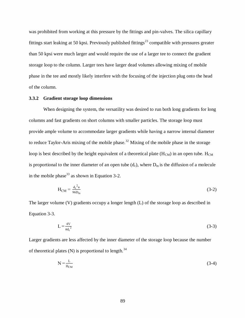
89
was prohibited from working at this pressure by the fittings and pin-valves. The silica capillary
fittings start leaking at 50 kpsi. Previously published fittings23
compatible with pressures greater
than 50 kpsi were much larger and would require the use of a larger tee to connect the gradient
storage loop to the column. Larger tees have larger dead volumes allowing mixing of mobile
phase in the tee and mostly likely interfere with the focusing of the injection plug onto the head
of the column.
3.3.2 Gradient storage loop dimensions
When designing the system, the versatility was desired to run both long gradients for long
columns and fast gradients on short columns with smaller particles. The storage loop must
provide ample volume to accommodate larger gradients while having a narrow internal diameter
to reduce Taylor-Aris mixing of the mobile phase.32
Mixing of the mobile phase in the storage
loop is best described by the height equivalent of a theoretical plate (HCM) in an open tube. HCM
is proportional to the inner diameter of an open tube (dc), where Dm is the diffusion of a molecule
in the mobile phase33
as shown in Equation 3-2.
HCM dc
2u
6Dm (3-2)
The larger volume (V) gradients occupy a longer length (L) of the storage loop as described in
Equation 3-3.
L 4V
dc2 (3-3)
Larger gradients are less affected by the inner diameter of the storage loop because the number
of theoretical plates (N) is proportional to length.34
N L
HCM (3-4)

90
The derivation comparing band broadening for different storage loops and gradient
volumes can be found in table Table 3.3. For the larger, 125 μL, gradient, 23 theoretical plates
were calculated with a . 25 cm ID storage loop. For a shorter, 5 μL, gradient, there were only
91 theoretical plates. To achieve 2300 theoretical plates for the shorter gradient, a 0.0050 cm
storage loop had to be used. A balance must be made, however, between the internal diameter
and the practicality of the length of the storage loop. To provide storage of larger gradients
without compromising the integrity of shorter gradients two storage loops were used in tandem.
The first section was 10 m of 50 μm I.D. silica capillary, which stored 2 μL. The second section
was 10 m of 250 µm ID stainless steel tubing capable of storing 0.5 mL. As shown in Figure 3.2,
a linear gradient was not delivered with only the 250 µm ID storage loop installed. The 17 μL
gradient should produce a 56-min-long linear section from 4-40%B followed by a ramp to a
85%B wash. The red trace shows mixing of the gradient when it was loaded at 10 μL/min into
the 250 µm ID storage loop. The loading flow rate was reduced to 5 μL/min which slightly
improved the linearity of the delivered gradient (blue trace). The addition of the 50 μm ID silica
capillary produced a very linear, 56-minute-long gradient that was not mixed with the 85%B
wash (green trace). With the narrow ID storage loop inline, the desired gradient profiles were
delivered after storage in the loop.
3.3.3 Selecting the flow rate for gradient loading
The Hcm-term is also proportional to the linear velocity (u) making the flow rate (F)34
at
which the gradient was loaded an important parameter to study. The relationship is as follows:
u 4F
dc2 (3-5)
The effect of gradient loading flow rate is shown in Figure 3.2. When the gradient is loaded at 10
µL/min, the playback of the gradient is not as desired. Reducing the gradient loading flow rate to

91
5 µL/min improved the gradient profile as depicted in Figure 3.3.a. with the playback of
gradients of varying volumes. The time of the linear portion of the gradient profile was plotted
versus the gradient volume in Figure 3.3.b. The linear fit of the data produced an R2 value of
0.999. The equation of the line was y = 3.33x +4.19. The inverse slope was 0.300 µL/min and
corresponded to the playback flow rate.
3.3.4 Repeatability
The repeatability was accessed for a 12.5 µL gradient run at 30 kpsi and 65°C on a 110
cm x 75 µm ID column packed with 1.9 µm BEH C18 particles. Enolase was separated by this
method on twelve different days. The retention times are listed in Table 3.4 for peptides
identified in all the analyses. The mean ( ), standard deviation (s), and relative standard
deviations (%RSD) were calculated from these results. All peptides had retention times with a
4.5%RSD or less. The retention time residual for each peptide was calculated as the retention
time on a given day minus the average retention time. The residuals were plotted versus day of
analysis in Figure 3.4. On most days (replicates 1-6, 10 and 12), retention times vary by less than
two minutes from the mean. As evident from the tight clusters of data (except for replicates 1, 7
and 11), the retention time shifts were similar for all peaks on any given day. Since this is a
constant pressure system, longer retention times, for replicated 9 and 10, may be attributed to
partial clogging of the pigtail or spray tip after the column.
3.3.5 Elevated temperature separations
Though not a requirement for operating the system, there were several motivations to
heat the column to 65°C. Higher temperatures reduce the viscosity of the mobile phase.
Therefore, longer columns can be used without reducing flow rate and increasing analysis time at
a given pressure. The higher temperatures also reduced the change in mobile phase viscosity.

92
The gradient varied from 4-40% acetonitrile in water. Through the gradient, the viscosity and
flow rate would fluctuate by nearly 10% at 25°C but only 5% at 65°C.35,36,37
The resistance to
mass transfer is reduced at high temperatures which flattens the C-term portion of a Van
Deemter plot and consequently shifts optimal velocity to a higher value. Analysis time can then
be reduced because a separation with a higher flow rate will not suffer as great a loss of
theoretical plates when run at 65°C versus 25°C.34
3.3.6 Column selection
To test the performance capabilities of the UHPLC, columns of varying length with
several different particle diameters were selected. The internal column diameter was kept
constant at 75 µm to be compatible with the volume necessary for nanoESI. Before use the
column performance was evaluated by isocratic elution to confirm that all columns had similar
reduced Van Deemter terms which is evident in Figure 3.5. The h-min of the 28.5 cm x 75 µm
ID column with 1.1 µm BEH C18 stationary phase was slightly higher than the other columns
evaluated. However, 1.1 µm particles were difficult to pack, especially to a length of 28.5 cm,
and an h-min around 2.5 was very acceptable.
3.3.7 Separations at ultrahigh pressures
Once it was determined that the system delivered gradients as desired, separations were
conducted at a variety of gradient volumes as shown in Figure 3.6. Resolving power increased as
gradient volume increased for separations at 15 kpsi of the standard protein digest on a 44.1 cm x
75 µm, 1.4 µm BEH C18 column. From each of the chromatograms, a representative peak,
selected for its average intensity and retention time, was extracted and plotted in the insert of
Figure 3.6. As gradient volume increased, peak width increased and peak height decreased. This
same experiment was carried out at 15, 30 and 45 kpsi. Example chromatograms in Figure 3.7 of

93
a 56 µL gradient run at the three different pressures illustrated how run time decreased and flow
rate increased as the operating pressure increased. The insert in Figure 3.7 of a representative
peak from all three chromatograms showed how peak width decreased at higher pressure while
peak intensity remained constant.
A summary of the peak capacity data can be found in Table 3.5. The goal was to increase
gradient volumes until a leveling off of peak capacity versus separations window was observed.
As presented in Figure 3.8, the peak capacity from the separations at 45 kpsi plateaued at a lower
value than for the separations at 30 kpsi. The separations at 15 kpsi reached a higher maximum
peak capacity as compared to the higher pressure separations. At 15 kpsi, the linear velocity was
8 cm/min which is closer to the optimum velocity. At the higher pressures and flow rates, a
higher C-term contributed more to the band broadening.
To determine how a proteomics sample would behave on this column, the same methods
at various gradient volumes and pressures were used to separate the E. coli digestion standard.
Though example separations at 15 kpsi in Figure 3.9 were very busy, an increase in resolution
was observed as gradient volume increase which was indicated by the signal being closer to
baseline between adjacent peaks. The benefit of reduced run time at higher pressures is shown in
Figure 3.10 for a 56 µL gradient. In Figure 3.11, the number of E. coli peptide and protein
identifications are plotted versus the separation window in parts a and b, respectively. The
separations at 15 kpsi contained the most identifications followed by the separations at 30 kpsi
and then by 45 kpsi. The peptide identifications begin to level off with respect to time faster than
the protein identifications. For the shallowest gradients, peptide identifications actually start to
decrease which was mostly likely due to the decrease in peak intensity for long separations.
When the peptide identifications were plotted against peak capacity in part c, there was no strong

94
correlation. However, protein identifications were very linear when plotted against peak capacity
as can be seen in part d. Because the peak capacity always increased as the separation window
increased, the data points in parts c and d were still in order from smallest to largest gradient
volume when reading the graph from left to right.
Beyond measuring the number of protein identifications, it was also important to consider
productivity which can be described as protein identifications per minute. The highest
productivity measured was for the most aggressive gradient (4% change in mobile phase B per
column volume) at 45 kpsi, and the lowest productivity was observed for the shallowest gradient
(0.5% change in mobile phase B per column volume) at 15 kpsi. The productivity for all
separations was plotted in Figure 3.12. For high-throughput laboratories, the higher pressure
separations would be most useful.
3.3.8 Separations with long columns
The greatest benefit from having the ability to run ultrahigh pressure separations was
observed when running with a long column. In the red chromatogram in Figure 3.13, the
standard protein digest was separated on a 44.1 cm x 75 µm ID column with 1.9 µm BEH C18
particles at 15 kpsi. The blue trace was from a 30 kpsi separation of the same sample on a 98.2
cm x 75 µm ID column with 1.9 µm BEH C18 particles. By increasing the pressure, the flow
rates and run times were similar between the two separations. As evident from inset graph, the
width of a representative peak decreased at higher pressure yet peak intensity remained the same.
Several gradient volumes were run on the 98.2 cm column. The results are summarized in Table
3.5 and Figure 3.14 which also includes data from a shorter commercial column run on the
standard nanoAcquity. By increasing the operating pressure, the peak capacity increased for
separations on a longer column in the same amount of time as separations on a shorter column at
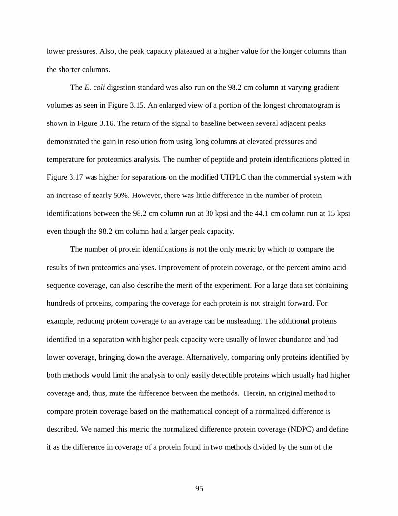
95
lower pressures. Also, the peak capacity plateaued at a higher value for the longer columns than
the shorter columns.
The E. coli digestion standard was also run on the 98.2 cm column at varying gradient
volumes as seen in Figure 3.15. An enlarged view of a portion of the longest chromatogram is
shown in Figure 3.16. The return of the signal to baseline between several adjacent peaks
demonstrated the gain in resolution from using long columns at elevated pressures and
temperature for proteomics analysis. The number of peptide and protein identifications plotted in
Figure 3.17 was higher for separations on the modified UHPLC than the commercial system with
an increase of nearly 50%. However, there was little difference in the number of protein
identifications between the 98.2 cm column run at 30 kpsi and the 44.1 cm column run at 15 kpsi
even though the 98.2 cm column had a larger peak capacity.
The number of protein identifications is not the only metric by which to compare the
results of two proteomics analyses. Improvement of protein coverage, or the percent amino acid
sequence coverage, can also describe the merit of the experiment. For a large data set containing
hundreds of proteins, comparing the coverage for each protein is not straight forward. For
example, reducing protein coverage to an average can be misleading. The additional proteins
identified in a separation with higher peak capacity were usually of lower abundance and had
lower coverage, bringing down the average. Alternatively, comparing only proteins identified by
both methods would limit the analysis to only easily detectible proteins which usually had higher
coverage and, thus, mute the difference between the methods. Herein, an original method to
compare protein coverage based on the mathematical concept of a normalized difference is
described. We named this metric the normalized difference protein coverage (NDPC) and define
it as the difference in coverage of a protein found in two methods divided by the sum of the

96
coverage. For example, consider the protein pyruvate kinase, which is involved in E. coli
glycolysis.38
For a 360 minute separation, pyruvate kinase had 47% coverage on the 98 cm
column and 27% coverage on the 44.1 cm column. The NDPC is 0.27 as calculated in
Equation 3-6.
NDPC Coverage1- Coverage2
Coverage1 Coverage2
4 -2
4 2 .2 (3-6)
The Normalized Difference Protein Coverage (NDPC) is plotted in Figure 3.18 for each
protein identified with the 360 minute gradient separation. If a protein was identified with higher
sequence coverage from the separation on the 98.2 cm column run at 30 kpsi, its NDPC value
was positive (blue bars). The red bars signified higher coverage with the separation on the 44.1
cm column at 15 kpsi. Proteins were plotted in order of decreasing coverage i.e. proteins wither
higher coverage were plotted on the left and proteins with lower coverage on the right.
Differences in coverage were minimal for highly covered proteins. As protein coverage
decreased, more proteins had higher coverage with the 98.2 cm column. Similar comparisons
were made for the 90 minute and 180 minute gradient separations and can be found in
Appendix B.1. and Appendix B.2., respectively. To provide a better visual of the trend in
coverage, the protein identifiers were removed from the graphs, and the NDPC were plotted in
Figure 3.19. parts a, b, and c for the 90, 180, and 360 minute gradient separations, respectively.
As evident by the larger portion of blue bars in part c, the greatest improvement in coverage
between the long and shorter column was with shallowest gradient.
In an attempt to further simplify the comparison of coverage between multiple methods,
while maintaining the meaning of the values, we propose the Grand NDPC which is calculated
by the difference between the grand total protein coverage in method one and method two

97
normalized by the grand sum of protein coverage in both methods. A formula for the Grand
NDPC is shown in Equation 3-7:
rand NDPC (∑Coverage
method 1)-(∑Coverage
method 2)
∑Coveragemethod 1
∑Coveragemethod 2
(3-7)
Perhaps a more relevant interpretation of the Grand NDPC would be to relate it to a fold-
change improvement in coverage as follows:
Fold-Change in Coverage ∑Coverage
method 1
∑Coveragemethod 2
1 rand NDPC
1- rand NDPC (3-8)
If the Fold-Change was less than one, the negative reciprocal of the value was used as is
conventional with fold-change calculations. The Grand NDPC and Fold-Change in Coverage is
listed in Table 3.6 for the E. coli digest standard 90, 180, and 360 min gradient separations on the
98.2 cm column run at 30 kpsi and the 44.1 cm column at 15 kpsi. Positive values represented
higher coverage on the long column, and negative values represented higher coverage on the
shorter column. Grand NDPC and Fold-Change Coverage increased in favor of the long column
as gradient length increased.
3.3.9 Separations with smaller particles
The last variable that was evaluated on the UHPLC was the use of columns with smaller
particles. Flow rate, running pressure, and column diameter were kept constant for these
experiments. Column length was shortened to compensate for the additional back pressure
necessary for running with smaller particles. The standard protein digest was separated on a 39.2
cm x 75 µm ID column packed with 1.4 µm BEH C18 particles at increasing gradient volumes as
shown in Figure 3.20. The inlaid graph depicted a representative peak. Similar to separations
shown for columns previously discussed in the chapter, the peak width increased and peak height
decreased as gradient volume increased. The smallest particles tested were 1.1 µm BEH C18

98
packed into a 28.5 cm x 75 µm ID column. These separations are shown in Figure 3.21. The
inset graph of the representative peak had a width of 0.1 minute for the fastest gradient which
was the narrowest width of any peak shown in this chapter. The peak width increased to 0.26
minutes for the slowest gradient on this column. A summary of the peak capacities are listed in
Table 3.5 and plotted in Figure 3.22. The red line represents separations at 30 kpsi on a 39.2 cm
x 75 µm ID column with 1.4 µm BEH C18 particles. The blue line represents separations on a
98.2 cm x 75 µm ID column with 1.9 µm BEH C18 particles. The green line represents
separations on a 28.5 cm x 75 µm ID column with 1.1 µm BEH C18 particles. The black line
represents separations on a commercial UPLC with a commercial column. The highest peak
capacities were achieved with the longest column and the largest particles. Even for very short
analysis times, peak capacities were higher with an aggressive gradient on a long column than a
shallower gradient on a shorter column packed with smaller particles. Pressure requirements
were proportional to length and inversely proportional to the particle diameter cubed. Therefore,
length had to be sacrificed when running a column with smaller particles which resulted in the
lower peak capacities.
The 39.2 cm x 75 µm ID column packed with 1.4 µm BEH C18 particles was also run at
15 and 45 kpsi as represented in Appendix B.3. The E. coli digestion standard was also analyzed
at all these conditions with example chromatograms shown in the Appendix B.4. and
Appendix B.5. The results are summarized in Table 3.5. Conclusions from this data were similar
to that discussed in the “Separations at ultrahigh pressures” section. The 28.5 cm x 5 µm ID
column with 1.1 µm BEH C18 particles broke before the E. coli digestion standard was
analyzed. There were not enough particles to pack another column with similar performance.

99
3.3.10 Literature comparison
Several labs have employed longer columns and ultrahigh pressures to improve peak
capacity and number of identifications for proteomic analyses. A representation of this work
from the literature, data from the commercial system, and data from this chapter are plotted in
Figure 3.23. The Marto group at Harvard39
packed 5 µm particles into a long narrow capillary of
100 cm x 25 µm ID and ran on a commercial system at 8 kpsi nominal back pressure. The Smith
group at PNNL24
separated peptides on three different columns at 20 kpsi. The column length
decreased to accommodate for the pressure required to use smaller particles. Data from this
chapter collected at 30 kpsi with the 98.2 cm x 75 µm ID column packed with 1.9 µm BEH C18
particles outperformed the results found in the literature in less times.
3.4 Conclusions
A gradient elution system capable of 45 kpsi has been developed to improve the separation of
proteomic samples. By implementing longer columns and smaller particles, the peak capacity
and productivity were increased. The peak capacities achieved with this system for a standard
peptide mixture ranged from 174 in 22 minutes for fast, steep gradients and 773 in 360 minutes
for slower shallower gradients. The highest peak capacities were achieved with the longest
column. Even for very short analyses, peak capacities were higher for an aggressive gradient on
a long column than a shallower gradient on a shorter column with smaller particles. The peak
capacities associated with this system led to increased protein identifications and sequence
coverage.
This instrument would be well suited to perform the second dimension separations in a
prefractionation-type multidimensional proteomics separation7 or as the first dimension followed

100
by a fast separation on a microchip.40
The improved separation efficiency available through this
ultrahigh pressure system could prove useful in other –omics research such as metabolomics.

101
3.5 TABLES
Time
(min)
Flow
Rate
(µL/min)
% Mobile
Phase A
% Mobile
Phase A Curve
NanoAcquity
Vent Valve
High Pressure Isolation Valve
Freeze/Thaw Valve
Vent Valve
Pneumatic Amplier
Pump Initiation
Gradient Loading Method
Initial 5 96.0 4.0 - Off On Off
1.0 5 15.0 85 11 Off On Off 1.8 5 60.0 40 11 Off On Off
x + 1.8 5 96.0 4 6 Off On Off x + 2.4 5 99.5 0.5 11 Off On Off x + 4.0 4 99.5 0.5 11 Off On Off x + 4.1 3 99.5 0.5 11 Off On Off x + 4.2 2 99.5 0.5 11 Off On Off x + 4.3 1 99.5 0.5 11 Off On Off x + 4.4 0.01 99.5 0.5 11 Off On Off
x + 5.0 (end) 0.01 99.5 0.5 11 Off On Off
Sample Loading Method
Initial 0.01 99.5 0.5 - Off On Off
0.1 1 99.5 0.5 11 Off On Off 0.2 2 99.5 0.5 11 Off On Off 0.3 3 99.5 0.5 11 Off On Off 0.4 4 99.5 0.5 11 Off On Off 0.5 5 99.5 0.5 11 Off On Off 2.0 5 99.5 0.5 11 Off On Off 2.5 0.01 50 50 11 On Off Off 5.0 0.01 50 50 11 On Off On
Ultra High Pressure Separation Method
Initial 0.01 50 50 11 On Off On y 0.01 96 4 11 On On Off
y + 5.0 (end) 0.01 96 4 11 On On Off
Table 3.1. The methods as programmed into MassLynx were listed along with the valve timings. The gradient loading time was listed
as x, where x equals the gradient volume divided by the flow rate when loading the gradient. The time to play back the gradient was
listed as y.

102
Column A Column B Column C Column D
Column Length
(cm) 44.1 98.2 39.2 28.5
Internal Diameter
(µm) 75 75 75 75
Particle Diamter
(µm) 1.9 1.9 1.4 1.1
Flow Rate (nL/min)
Pressure
15kpsi 350 - 190 -
30kpsi 730 330 410 370
45kpsi 1160 - 610 -
Gradient Volume (µL)
Percent
Change MPB
Per Column
Volume
4.0% 14 31 12.5 8
2.0% 28 62 25 16
1.0% 56 124 50 31
0.5% 113 249 100 62
Table 3.2. The dimensions for each of the analytical columns tested in this manuscript were
listed along with their measured flow rates and programmed gradient volumes.

103
Gradient Volume, V, (μL) 125 5.0 5.0
Inner Diameter, dc, (cm) 0.025 0.025 0.0050
Gradient Loading
Flow Rate, F, (μL/min)
5.0 5.0 5.0
Linear Velocity, (cm/s)
0.17 0.17 4.2
HETP (cm)
0.11 0.11 0.11
Gradient Length (cm)
250 10 250
Number of Plates
2300 91 2300
Table 3.3. The number of theoretical plates was calculated for several gradient storage loop
internal diameters and gradient volumes.
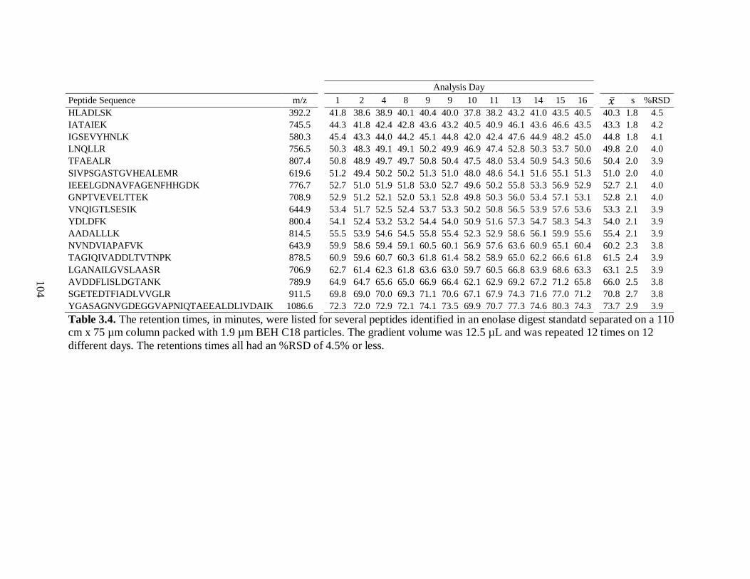
104
Analysis Day
Peptide Sequence m/z
1 2 4 8 9 9 10 11 13 14 15 16 s %RSD
HLADLSK 392.2
41.8 38.6 38.9 40.1 40.4 40.0 37.8 38.2 43.2 41.0 43.5 40.5
40.3 1.8 4.5
IATAIEK 745.5
44.3 41.8 42.4 42.8 43.6 43.2 40.5 40.9 46.1 43.6 46.6 43.5
43.3 1.8 4.2
IGSEVYHNLK 580.3
45.4 43.3 44.0 44.2 45.1 44.8 42.0 42.4 47.6 44.9 48.2 45.0
44.8 1.8 4.1
LNQLLR 756.5
50.3 48.3 49.1 49.1 50.2 49.9 46.9 47.4 52.8 50.3 53.7 50.0
49.8 2.0 4.0
TFAEALR 807.4
50.8 48.9 49.7 49.7 50.8 50.4 47.5 48.0 53.4 50.9 54.3 50.6
50.4 2.0 3.9
SIVPSGASTGVHEALEMR 619.6
51.2 49.4 50.2 50.2 51.3 51.0 48.0 48.6 54.1 51.6 55.1 51.3
51.0 2.0 4.0
IEEELGDNAVFAGENFHHGDK 776.7
52.7 51.0 51.9 51.8 53.0 52.7 49.6 50.2 55.8 53.3 56.9 52.9
52.7 2.1 4.0
GNPTVEVELTTEK 708.9
52.9 51.2 52.1 52.0 53.1 52.8 49.8 50.3 56.0 53.4 57.1 53.1
52.8 2.1 4.0
VNQIGTLSESIK 644.9
53.4 51.7 52.5 52.4 53.7 53.3 50.2 50.8 56.5 53.9 57.6 53.6
53.3 2.1 3.9
YDLDFK 800.4
54.1 52.4 53.2 53.2 54.4 54.0 50.9 51.6 57.3 54.7 58.3 54.3
54.0 2.1 3.9
AADALLLK 814.5
55.5 53.9 54.6 54.5 55.8 55.4 52.3 52.9 58.6 56.1 59.9 55.6
55.4 2.1 3.9
NVNDVIAPAFVK 643.9
59.9 58.6 59.4 59.1 60.5 60.1 56.9 57.6 63.6 60.9 65.1 60.4
60.2 2.3 3.8
TAGIQIVADDLTVTNPK 878.5
60.9 59.6 60.7 60.3 61.8 61.4 58.2 58.9 65.0 62.2 66.6 61.8
61.5 2.4 3.9
LGANAILGVSLAASR 706.9
62.7 61.4 62.3 61.8 63.6 63.0 59.7 60.5 66.8 63.9 68.6 63.3
63.1 2.5 3.9
AVDDFLISLDGTANK 789.9
64.9 64.7 65.6 65.0 66.9 66.4 62.1 62.9 69.2 67.2 71.2 65.8
66.0 2.5 3.8
SGETEDTFIADLVVGLR 911.5
69.8 69.0 70.0 69.3 71.1 70.6 67.1 67.9 74.3 71.6 77.0 71.2
70.8 2.7 3.8
YGASAGNVGDEGGVAPNIQTAEEALDLIVDAIK 1086.6
72.3 72.0 72.9 72.1 74.1 73.5 69.9 70.7 77.3 74.6 80.3 74.3
73.7 2.9 3.9
Table 3.4. The retention times, in minutes, were listed for several peptides identified in an enolase digest standatd separated on a 110
cm x 75 µm column packed with 1.9 µm BEH C18 particles. The gradient volume was 12.5 µL and was repeated 12 times on 12
different days. The retentions times all had an %RSD of 4.5% or less.

105
Column
Description
Pressure
(kpsi)
Gradient Length
(%B per
Column Volume)
Separation
Window
(min)
Average
Peak Width
(min)
Peak
Capacity
Protein
IDs
Peptide
ID
25 cm x
75 µm ID
1.9 µm dp
8
4 15 0.17 88 111 1060
2 30 0.29 103 169 1540
1 60 0.37 161 201 1876
0.5 120 0.92 191 196 1493
44.1 cm x
75 µm ID
1.9 µm dp
15
4 35 0.13 264 207 2534
2 69 0.18 385 255 2982
1 132 0.29 455 302 3127
0.5 275 0.46 596 362 2742
30
4 18 0.10 174 156 1652
2 34 0.14 254 199 2048
1 67 0.18 379 232 2029
0.5 137 0.32 433 260 2020
45
4 11 0.09 125 127 1371
2 24 0.14 174 166 1664
1 47 0.18 269 212 1984
0.5 93 0.27 344 238 1990
98.2 cm x
75 µm ID
1.9 µm dp
30
4 90 0.20 457 265 2682
2 180 0.29 622 290 2868
1 360 0.47 773 395 2883
0.5 720 0.82 877 343 2003
39.2 cm x
75 µm ID
1.4 µm dp
15
4 67 0.21 316 222 3038
2 113 0.29 385 263 3363
1 198 0.41 482 291 3160
0.5 400 0.55 724 232 1775
30
4 34 0.14 246 184 2347
2 60 0.17 352 273 3346
1 123 0.34 366 321 3758
0.5 240 0.42 566 359 2711
45
4 21 0.10 215 147 1502
2 42 0.15 293 178 1786
1 83 0.23 376 223 2030
0.5 162 0.34 481 193 1460
28.5 cm x
75 µm ID
1.1 µm dp
30
4 22 0.13 174
n/a n/a 2 38 0.17 220
1 70 0.23 309
0.5 125 0.36 352
Table 3.5. The average separation window, peak width (4σ), peak capacity, and number of
protein and peptide identifications were listed for each column at each running condition.

106
Gradient Length (min) Grand NDPC Fold-Change Coverage
90 -0.0050 -1.01
180 0.057 1.12 360 0.10 1.22
Table 3.6. The Grand NDPC and Fold-Change Coverage were compared for E. coli digest
separated on the 98.2 cm column run at 30 kpsi to the 44.1 cm column run at 15 kpsi for three
gradient lengths. Positive values represented higher coverage on the long column, and negative
values represented higher coverage on the shorter column. Grand NDPC and Fold-Change
Coverage increased in favor of the long column as gradient length increased.

107
3.6 FIGURES
Figure 3.1. The nanoAcquity is shown with the additional tubing and valves necessary for
separations at 45 kpsi driven by the Haskel pneumatic amplifier pump.

108
Figure 3.2. The gradient playback time of the UHPLC was monitored by the UV absorbance of
acetone in mobile phase B. The gradient linearity was improved by using a lower flow rate for
gradient loading and employing the 50 µL ID tubing at the head of the gradient storage loop.

109
a)
b)
Figure 3.3. The gradient playback time of the UHPLC was monitored by the UV absorbance of
acetone in mobile phase B and plotted in part (a) for several different gradient volumes which
were noted on the graph. The playback time of the linear region was plotted versus gradient
volume in part (b). A best fit line had the equation y = 3.33x – 4.19 and R2 value of 0.999. The
inverse slope was 0.300 µL/min which corresponded to flow rate.
100
80
60
40
20
0
%B
25020015010050
Time (min)
4µL 17µL10µL 33µL 53µL
Gradient Volumes
160
140
120
100
80
60
40
20
Pla
yb
ack
Tim
e (m
in)
5040302010
Gradient Volume (µL)
y = 3.33x - 4.19
R² = 0.999
Inverse Slope = 0.300 µL/min
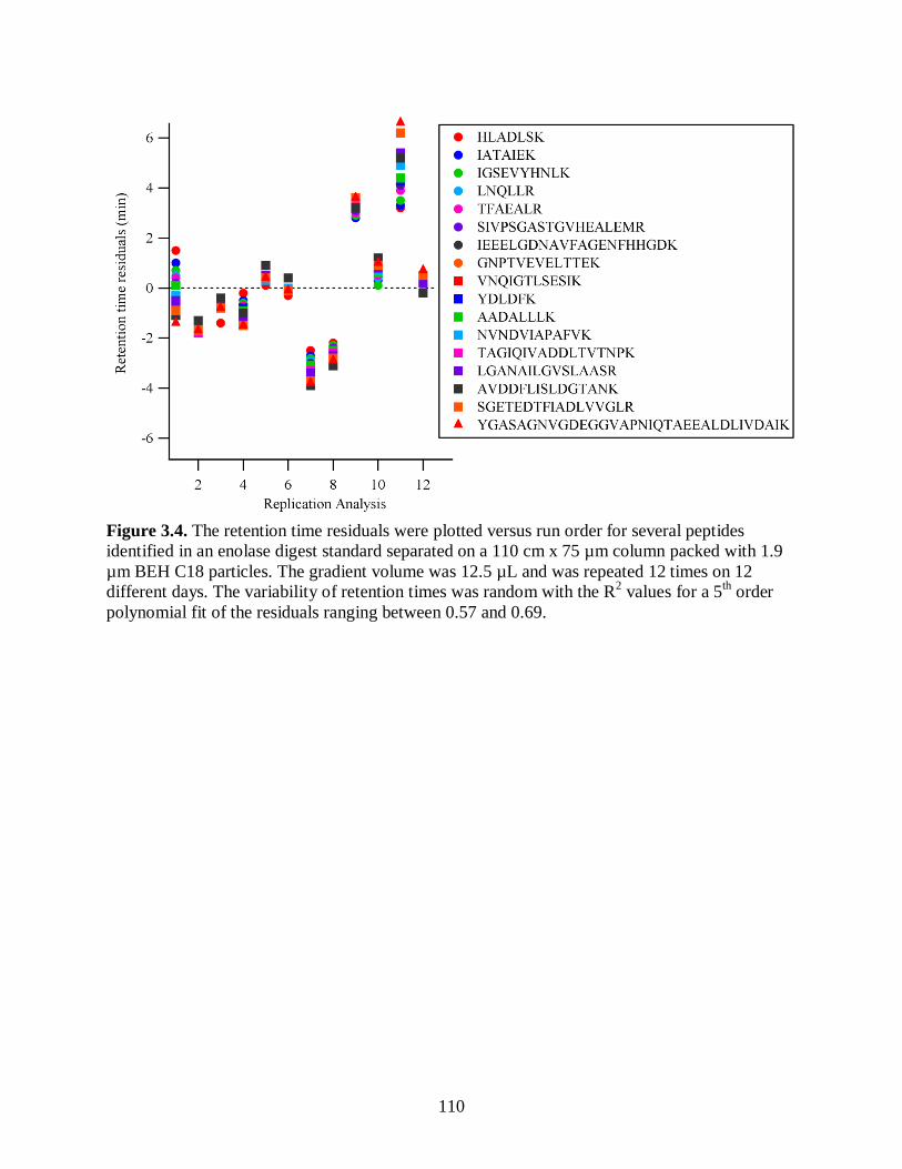
110
Figure 3.4. The retention time residuals were plotted versus run order for several peptides
identified in an enolase digest standard separated on a 110 cm x 75 µm column packed with 1.9
µm BEH C18 particles. The gradient volume was 12.5 µL and was repeated 12 times on 12
different days. The variability of retention times was random with the R2 values for a 5
th order
polynomial fit of the residuals ranging between 0.57 and 0.69.

111
Figure 3.5. The Van Deemter plots with reduced terms of hydroquinone demonstrate the
similarity in column performance for the columns tested in these experiments.
4
3
2
1
0
h
86420
ν
28.5 cm x 75 µm, 1.1 µm BEH C18
98.2 cm x 75 µm, 1.9 µm BEH C18
44.1 cm x 75 µm, 1.9 µm BEH C18
39.2 cm x 75 µm, 1.4 µm BEH C18
112
Figure 3.6. Chromatograms of MassPREPTM
Digestion Standard Protein Expression Mixture 2
were collected for separations with increasing gradient volume on the 44.1 cm x 75 µm ID
column packed with 1.9 µm BEH C18 particles. Separations were completed at 15 kpsi. The
insert of a representative peptide peak with 724 m/z extracted from all four chromatograms
demonstrated the increase in peak width and decrease in peak height as the as gradient volume
increased.

113
150
100
50
0
31.831.631.4
724 m/z
Figure 3.7. Chromatograms of MassPREPTM
Digestion Standard Protein Expression Mixture 2
were collected for separations with increasing pressure and flow rate on the 44.1 cm x 75 µm ID
column packed with 1.9 µm BEH C18 particles. Separations were completed with a 56 µL
gradient volume. The insert of a representative peptide peak with 724 m/z extracted from all
three chromatograms showed the decrease in peak width and constant signal intensity as pressure
and flow rate increased.
1200
1000
800
600
400
200
BP
I
120100806040200
Time (min)
45 kpsi, 1160 nL/min
30 kpsi, 730 nL/min
56 µL Gradient Volume
1% Change MPB per Column Volume
15 kpsi, 350 kpsi
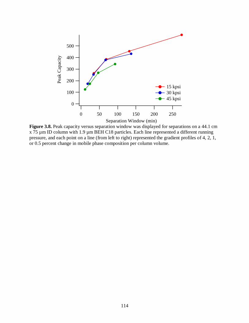
114
Figure 3.8. Peak capacity versus separation window was displayed for separations on a 44.1 cm
x 75 µm ID column with 1.9 µm BEH C18 particles. Each line represented a different running
pressure, and each point on a line (from left to right) represented the gradient profiles of 4, 2, 1,
or 0.5 percent change in mobile phase composition per column volume.
500
400
300
200
100
0
Pea
k C
apac
ity
250200150100500
Separation Window (min)
15 kpsi
30 kpsi
45 kpsi

115
Figure 3.9. Chromatograms of MassPREPTM
E. coli Digestion Standard were collected for
separations with increasing gradient volume on the 44.1 cm x 75 µm ID column packed with 1.9
µm BEH C18 particles. Separations were completed at 15 kpsi. Though the chromatograms were
very busy, an increase in resolution was observed as gradient volume increased which was
indicated by the signal being closer to baseline between two adjacent peaks.
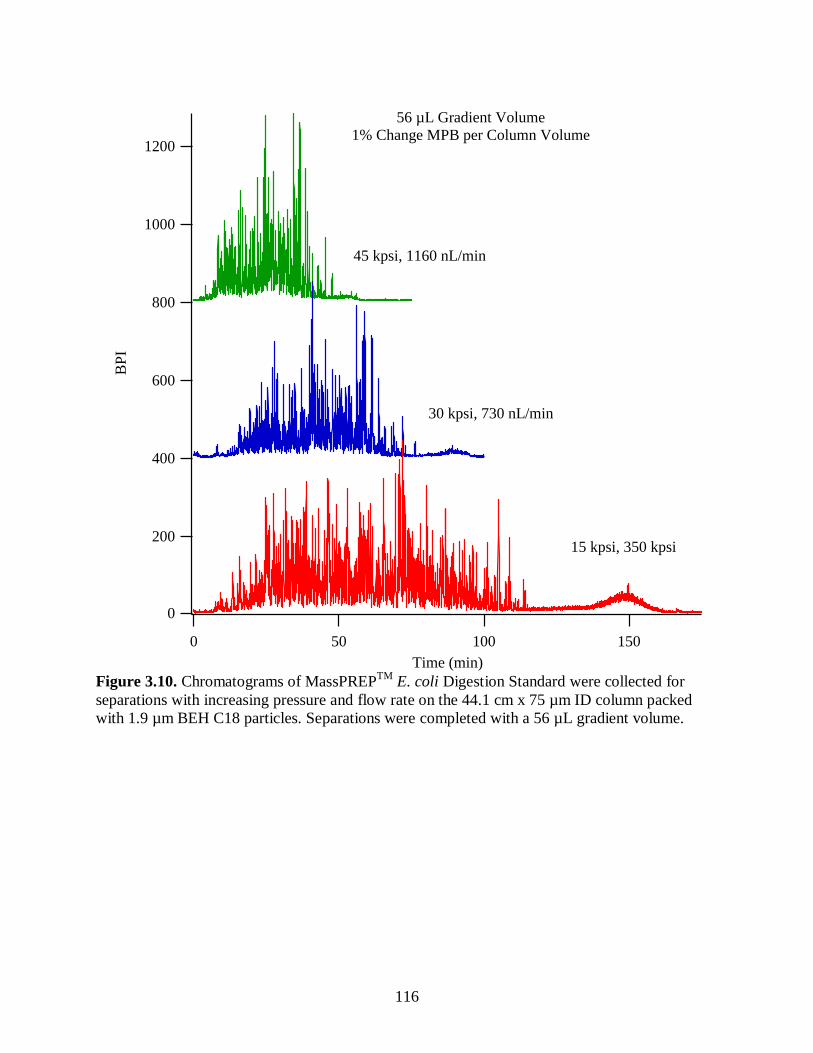
116
Figure 3.10. Chromatograms of MassPREP
TM E. coli Digestion Standard were collected for
separations with increasing pressure and flow rate on the 44.1 cm x 75 µm ID column packed
with 1.9 µm BEH C18 particles. Separations were completed with a 56 µL gradient volume.
1200
1000
800
600
400
200
0
BP
I
150100500
Time (min)
45 kpsi, 1160 nL/min
30 kpsi, 730 nL/min
56 µL Gradient Volume
1% Change MPB per Column Volume
15 kpsi, 350 kpsi

117
a) b)
c) d)
Figure 3.11. The peptide and protein identifications for E. coli were plotted versus the separation
window and peak capacity for several separations on a 44.1 cm x 75 µm ID column with 1.9 µm
BEH C18 particles. Each line represents a different running pressure, and each point on a line
(from left to right) represented the gradient profiles of 4, 2, 1, or 0.5 percent change in mobile
phase per column volume.
3000
2500
2000
1500
1000
500
0
E. co
li P
epti
de
IDs
250200150100500
Separation Window (min)
350
300
250
200
150
100
50
0
E. co
li P
rote
in I
Ds
250200150100500
Separation Window (min)
3000
2500
2000
1500
1000
500
0
E.
coli
Pep
tid
e ID
s
5004003002001000
Peak Capacity
350
300
250
200
150
100
50
0
E. co
li P
rote
in I
Ds
5004003002001000
Peack Capacity
15 kpsi
30 kpsi
45 kpsi

118
Figure 3.12. Protein identifications per minute or productivity was plotted for the E. coli protein
identifications from analyses at varying gradient volumes and pressures on the 44.1 cm x 75 µm
ID column with 1.9 µm BEH C18 particles. Productivity was highest for the steepest gradient
run at the highest pressure.
12
10
8
6
4
2
0
Pro
tein
Id
enti
fica
tio
ns
per
Min
ute
4% 2% 1% 0.5%Mobile Phase Change per Column Volume
39.2 cm x 75 um, 1.4 um BEH
45 kpsi
30 kpsi
15 kpsi
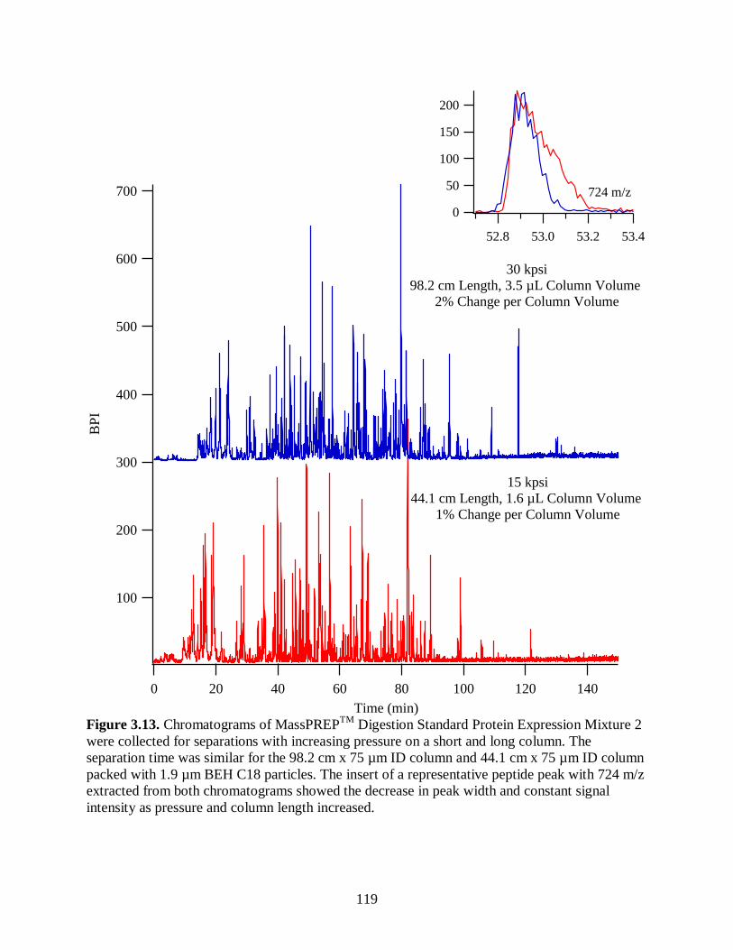
119
200
150
100
50
0
53.453.253.052.8
724 m/z
Figure 3.13. Chromatograms of MassPREP
TM Digestion Standard Protein Expression Mixture 2
were collected for separations with increasing pressure on a short and long column. The
separation time was similar for the 98.2 cm x 75 µm ID column and 44.1 cm x 75 µm ID column
packed with 1.9 µm BEH C18 particles. The insert of a representative peptide peak with 724 m/z
extracted from both chromatograms showed the decrease in peak width and constant signal
intensity as pressure and column length increased.
700
600
500
400
300
200
100
BP
I
140120100806040200
Time (min)
30 kpsi
98.2 cm Length, 3.5 µL Column Volume
2% Change per Column Volume
15 kpsi
44.1 cm Length, 1.6 µL Column Volume
1% Change per Column Volume

120
Figure 3.14. The increasing peak capacity versus separation window plot demonstrated the
benefit of using higher pressures to run longer columns in the same amount of time as shorter
columns. The red line represented separations at 15 kpsi on a 44.1 cm x 75 µm ID column with
1.9 µm BEH C18 particles. The blue line represented separations at 30 kpsi on a 98.2 cm x 75
µm ID column with 1.9 µm BEH C18 particles. The gray line represented separations on a
commercial UPLC with a commercial column (25 cm x 75 µm ID column with 1.9 µm BEH C18
particles). Each point on a line (from left to right) represented the gradient profiles of 4, 2, 1, or
0.5 percent change in mobile phase per column volume.
800
600
400
200
0
Pea
k C
apac
ity
7006005004003002001000
Separation Window (min)
98 cm x 75 µm, 1.9 µm BEH C18
30 kpsi, 330 nL/min
44 cm x 75 µm, 1.9 µm BEH C18
15 kpsi, 350 nL/min
25 cm x 75 µm, 1.9 µm BEH C18
8 kpsi, 300 nL/min

121
Figure 3.15. Chromatograms of MassPREPTM
E. coli Digestion Standard were collected for
separations with increasing gradient volume on the 98.2 cm x 75 µm ID column packed with 1.9
µm BEH C18 particles. Separations were completed at 30 kpsi. Though the chromatograms were
very busy, an increase in resolution was observed as gradient volume increased which was
indicated by the signal being closer to baseline between two adjacent peaks. These were the
shotgun proteomic experiments with the highest peak capacities.

122
Figure 3.16. This chromatogram of MassPREPTM
E. coli Digestion Standard from the 98.2 cm x
75 µm ID column packed with 1.9 µm BEH C18 particles is a zoomed in version of the purple
chromatogram in Figure 3.15. The return of signal to baseline between several adjacent peaks
demonstrated the gain in resolution from using long columns at elevated pressures and
temperature for proteomics analysis.

123
a) b)
Figure 3.17. The peptide and protein identifications for E. coli were plotted versus the separation
window in parts a and b, respectively. The red line represented separations at 15 kpsi on a 44.1
cm x 75 µm ID column with 1.9 µm BEH C18 particles. The blue line represented separations at
30 kpsi on a 98.2 cm x 75 µm ID column with 1.9 µm BEH C18 particles. The gray line
represented separations on a commercial UPLC with a commercial column (25 cm x 75 µm ID
column with 1.9 µm BEH 18 particles). Each point on a line (from left to right) represented the
gradient profiles of 4, 2, 1, or 0.5 percent change in mobile phase per column volume.
3000
2500
2000
1500
1000
500
0
E. co
li P
epti
de
IDs
6004002000
Separation Window (min)
300
200
100
0
E.
coli
Pro
tein
ID
s
6004002000
Separation Window (min)
98 cm x 75 µm, 1.9 µm BEH C18
30 kpsi, 330 nL/min
44 cm x 75 µm, 1.9 µm BEH C18 15 kpsi, 350 nL/min
25 cm x 75 µm, 1.9 µm BEH C18
8 kpsi, 300 nL/min

124
Figure 3.18. The NDPC comparing the analysis on the 98.2 cm column run at 30 kpsi to the 44.1
cm column run at 15 kpsi for a 360 min gradient was plotted for each protein identified in an E.
coli digest standard. If a protein was identified with higher sequence coverage with the
separation on the 98.2 cm column, its NDPC value was positive (blue bars). The red bars
signified higher coverage with the separation on the 44.1 cm column. Proteins with higher
coverage were plotted on the left, and proteins with lower coverage were on the right.
Differences in coverage were minimal for highly covered proteins. As protein coverage
decreased, more proteins were identified with higher coverage with the separation on the 98.2 cm
column. The dashed line represented a two-fold difference in protein coverage.

125
Figure 3.18. (continued)

126
Figure 3.18. (continued)

127
a)
b)
c)
Figure 3.19. The NDPC comparing the analysis on the 98.2 cm column run at 30 kpsi to the 44.1
cm column run at 15 kpsi was plotted for each protein identified in an E. coli digest standard
separated with a for a 90 min (part a), 180 min (part b), and 360 min (part c) gradient . If a
protein was identified with higher sequence coverage with the separation on the 98.2 cm column,
its NDPC value was positive (blue bars). The red bars signified higher coverage with the
separation on the 44.1 cm column. Proteins with higher coverage were plotted on the left, and
proteins with lower coverage were on the right. Differences in coverage were minimal for highly
covered proteins. As protein coverage decreased, more proteins were identified with higher
coverage with the separation on the 98.2 cm column.
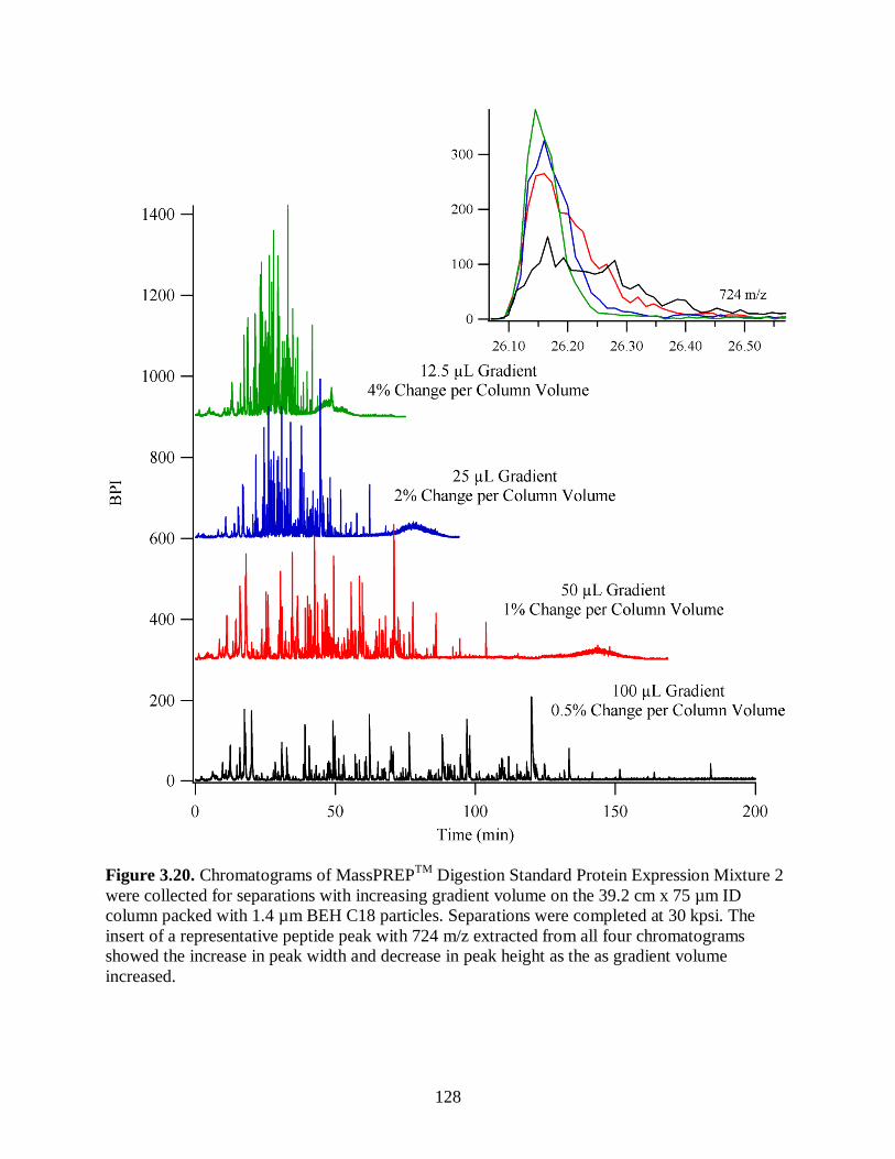
128
Figure 3.20. Chromatograms of MassPREPTM
Digestion Standard Protein Expression Mixture 2
were collected for separations with increasing gradient volume on the 39.2 cm x 75 µm ID
column packed with 1.4 µm BEH C18 particles. Separations were completed at 30 kpsi. The
insert of a representative peptide peak with 724 m/z extracted from all four chromatograms
showed the increase in peak width and decrease in peak height as the as gradient volume
increased.
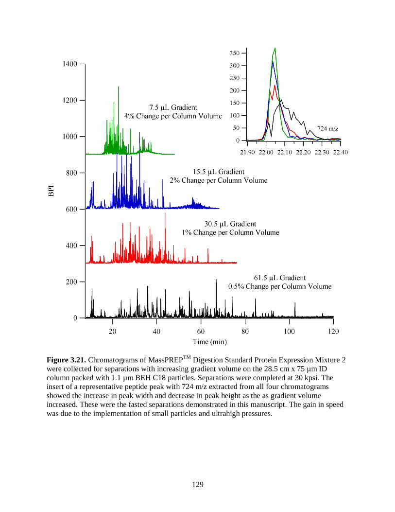
129
Figure 3.21. Chromatograms of MassPREPTM
Digestion Standard Protein Expression Mixture 2
were collected for separations with increasing gradient volume on the 28.5 cm x 75 µm ID
column packed with 1.1 µm BEH C18 particles. Separations were completed at 30 kpsi. The
insert of a representative peptide peak with 724 m/z extracted from all four chromatograms
showed the increase in peak width and decrease in peak height as the as gradient volume
increased. These were the fasted separations demonstrated in this manuscript. The gain in speed
was due to the implementation of small particles and ultrahigh pressures.

130
Figure 3.22. The increasing peak capacity versus separation window plot demonstrated the
difference in performance for columns with different particle sizes. The red line represented
separations at 30 kpsi on a 39.2 cm x 75 µm ID column with 1.4 µm BEH C18 particles. The
blue line represented separations on a 98.2 cm x 75 µm ID column with 1.9 µm BEH C18
particles. The green line represented separations on a 28.5 cm x 75 µm ID column with 1.1 µm
BEH C18 particles. The gray line represented separations on a commercial UPLC with a
commercial column.
800
600
400
200
0
Pea
k C
apac
ity
7006005004003002001000
Separation Window (min)
98.2 cm x 75 um, 1.9 µm BEH 30kpsi
39.2 cm x 75 um, 1.4 µm BEH 30kpsi
28.5 cm x 75 um, 1.1 µm BEH 30kpsi
25.0 cm x 75 um, 1.9 µm BEH 8kpsi

131
Figure 3.23. The peak capacity versus separation window plot compared the highest peak
capacities demonstrated in this manuscript, as obtained with the 98.2 cm x 75 µm ID column
with 1.9 µm BEH C18 particles, separations on the commercial nanoAcquity and several data
sets found in the literature for separations with long columns and at high pressure
(PNNL24
,Harvard39
). The data presented in this manuscript achieved higher peak capacities in
less time as compared to the literature data.

132
3.7 REFERENCES
1. Paik, Y.-K.; Jeong, S.-K.; Omenn, G. S.; Uhlen, M.; Hanash, S.; Cho, S. Y.; Lee, H.-J.;
Na, K.; Choi, E.-Y.; Yan, F.; Zhang, F.; Zhang, Y.; Snyder, M.; Cheng, Y.; Chen, R.;
Marko-Varga, G.; Deutsch, E. W.; Kim, H.; Kwon, J.-Y.; Aebersold, R.; Bairoch, A.;
Taylor, A. D.; Kim, K. Y.; Lee, E.-Y.; Hochstrasser, D.; Legrain, P.; Hancock, W. S.,
The Chromosome-Centric Human Proteome Project for cataloging proteins encoded in
the genome. Nat Biotech 2012, 30 (3), 221-223.
2. Anderson, N. L.; Anderson, N. G., The Human Plasma Proteome: History, Character, and
Diagnostic Prospects. Molecular & Cellular Proteomics 2003, 2 (1), 50.
3. Xie, F.; Smith, R. D.; Shen, Y., Advanced proteomic liquid chromatography. Journal of
Chromatography A 2012, 1261 (0), 78-90.
4. Yates, J. R.; Ruse, C. I.; Nakorchevsky, A., Proteomics by Mass Spectrometry:
Approaches, Advances, and Applications. Annual Review of Biomedical Engineering
2009, 11 (1), 49-79.
5. Washburn, M. P.; Ulaszek, R.; Deciu, C.; Schieltz, D. M.; Yates, J. R., Analysis of
Quantitative Proteomic Data Generated via Multidimensional Protein Identification
Technology. Analytical Chemistry 2002, 74 (7), 1650-1657.
6. Wolters, D. A.; Washburn, M. P.; Yates, J. R., An Automated Multidimensional Protein
Identification Technology for Shotgun Proteomics. Analytical Chemistry 2001, 73 (23),
5683-5690.
7. Stobaugh, J. T.; Fague, K. M.; Jorgenson, J. W., Prefractionation of Intact Proteins by
Reversed-Phase and Anion-Exchange Chromatography for the Differential Proteomic
Analysis of Saccharomyces cerevisiae. Journal of Proteome Research 2012, 12 (2), 626-
636.
8. Gilar, M.; Olivova, P.; Daly, A. E.; Gebler, J. C., Two-dimensional separation of peptides
using RP-RP-HPLC system with different pH in first and second separation dimensions.
Journal of Separation Science 2005, 28 (14), 1694-1703.
9. Emmett, M. R.; Caprioli, R. M., Micro-electrospray mass spectrometry: ultra-high-
sensitivity analysis of peptides and proteins. Journal of the American Society for Mass
Spectrometry 1994, 5 (7), 605-613.
10. Gale, D. C.; Smith, R. D., Small volume and low flow-rate electrospray lonization mass
spectrometry of aqueous samples. Rapid Communications in Mass Spectrometry 1993, 7
(11), 1017-1021.
11. Wilm, M. S.; Mann, M., Electrospray and Taylor-Cone theory, Dole's beam of
macromolecules at last? International Journal of Mass Spectrometry and Ion Processes
1994, 136 (2–3), 167-180.

133
12. Wilm, M.; Mann, M., Analytical Properties of the Nanoelectrospray Ion Source.
Analytical Chemistry 1996, 68 (1), 1-8.
13. Valentine, S. J.; Plasencia, M. D.; Liu, X.; Krishnan, M.; Naylor, S.; Udseth, H. R.;
Smith, R. D.; Clemmer, D. E., Toward Plasma Proteome Profiling with Ion Mobility-
Mass Spectrometry. Journal of Proteome Research 2006, 5 (11), 2977-2984.
14. FF, G.-G.; C, L.; SJ, H.; J, F.; C, B.; H, H.; AR, J., - A critical appraisal of techniques,
software packages, and standards for. D - 101131135 (- 1557-8100 (Electronic)), T -
ppublish.
15. Hebert, A. S.; Richards, A. L.; Bailey, D. J.; Ulbrich, A.; Coughlin, E. E.; Westphall, M.
S.; Coon, J. J., The One Hour Yeast Proteome. Molecular & Cellular Proteomics 2014,
13 (1), 339-347.
16. Annesley, T. M., Ion Suppression in Mass Spectrometry. Clinical Chemistry 2003, 49
(7), 1041-1044.
17. Giddings, J. C., Maximum number of components resolvable by gel filtration and other
elution chromatographic methods. Analytical Chemistry 1967, 39 (8), 1027-1028.
18. Giddings, J. C., Unified separation science. Wiley: 1991.
19. Neue, U. D., Theory of peak capacity in gradient elution. Journal of Chromatography A
2005, 1079 (1–2), 153-161.
20. Patel, K. D.; Jerkovich, A. D.; Link, J. C.; Jorgenson, J. W., In-Depth Characterization of
Slurry Packed Capillary Columns with 1.0-μm Nonporous Particles Using eversed-
Phase Isocratic Ultrahigh-Pressure Liquid Chromatography. Analytical Chemistry 2004,
76 (19), 5777-5786.
21. Liu, H.; Finch, J. W.; Lavallee, M. J.; Collamati, R. A.; Benevides, C. C.; Gebler, J. C.,
Effects of column length, particle size, gradient length and flow rate on peak capacity of
nano-scale liquid chromatography for peptide separations. Journal of Chromatography A
2007, 1147 (1), 30-36.
22. de Villiers, A.; Lestremau, F.; Szucs, R.; Gélébart, S.; David, F.; Sandra, P., Evaluation
of ultra performance liquid chromatography: Part I. Possibilities and limitations. Journal
of Chromatography A 2006, 1127 (1–2), 60-69.
23. MacNair, J. E.; Lewis, K. C.; Jorgenson, J. W., Ultrahigh-Pressure Reversed-Phase
Liquid Chromatography in Packed Capillary Columns. Analytical Chemistry 1997, 69
(6), 983-989.
24. Shen, Y.; Zhang, R.; Moore, R. J.; Kim, J.; Metz, T. O.; Hixson, K. K.; Zhao, R.;
Livesay, E. A.; Udseth, H. R.; Smith, R. D., Automated 20 kpsi RPLC-MS and MS/MS
with Chromatographic Peak Capacities of 1 −15 and Capabilities in Proteomics and
Metabolomics. Analytical Chemistry 2005, 77 (10), 3090-3100.

134
25. MacNair, J. E.; Patel, K. D.; Jorgenson, J. W., Ultrahigh-Pressure Reversed-Phase
Capillary Liquid Chromatography: Isocratic and radient Elution Using Columns
Packed with 1.0-μm Particles. Analytical Chemistry 1999, 71 (3), 700-708.
26. Link, J. C. Development and application of gradient ultrahigh pressure liquid
chromatography for separations of complex biological mixtures. The University of North
Carolina at Chapel Hill, 2004.
27. Eschelbach, J. W.; Jorgenson, J. W., Improved Protein Recovery in Reversed-Phase
Liquid Chromatography by the Use of Ultrahigh Pressures. Analytical Chemistry 2006,
78 (5), 1697-1706.
28. Gritti, F.; Guiochon, G., Theoretical comparison of the performance of gradient elution
chromatography at constant pressure and constant flow rate. Journal of Chromatography
A 2012, 1253 (0), 71-82.
29. Gritti, F.; Stankovich, J. J.; Guiochon, G., Potential advantage of constant pressure versus
constant flow gradient chromatography for the analysis of small molecules. Journal of
Chromatography A 2012, 1263 (0), 51-60.
30. Dourdeville, T. A. Peltier based freeze-thaw valves and method of use. US Patent
7,128,081. Oct 31, 2006.
31. WatersCorp. nanoAcuity UPLC System Instrument Specifications [Online], 2010, p.
720001083en.
32. Aris, R., On the Dispersion of a Solute in a Fluid Flowing through a Tube. Proceedings
of the Royal Society of London. Series A. Mathematical and Physical Sciences 1956, 235
(1200), 67-77.
33. Knox, J. H.; Gilbert, M. T., Kinetic optimization of straight open-tubular liquid
chromatography. Journal of Chromatography A 1979, 186 (0), 405-418.
34. Neue, U. D., HPLC Columns: Theory, Technology, and Practice. Wiley: 1997.
35. Chen, H.; Horváth, C., High-speed high-performance liquid chromatography of peptides
and proteins. Journal of Chromatography A 1995, 705 (1), 3-20.
36. Franklin, E. G. Utilization of Long Columns Packed with Sub-2 mum Particles Operated
at High Pressures and Elevated Temperatures for High-Efficiency One-Dimensional
Liquid Chromatographic Separations. The University of North Carolina at Chapel Hill,
2012.
37. Thompson, J. D.; Carr, P. W., High-Speed Liquid Chromatography by Simultaneous
Optimization of Temperature and Eluent Composition. Analytical Chemistry 2002, 74
(16), 4150-4159.

135
38. Yoshida, K.-i.; Yamaguchi, M.; Ikeda, H.; Omae, K.; Tsurusaki, K.-i.; Fujita, Y., The
fifth gene of the iol operon of Bacillus subtilis, iolE, encodes 2-keto-myo-inositol
dehydratase. Microbiology 2004, 150 (3), 571-580.
39. Zhou, F.; Lu, Y.; Ficarro, S. B.; Webber, J. T.; Marto, J. A., Nanoflow Low Pressure
High Peak Capacity Single Dimension LC-MS/MS Platform for High-Throughput, In-
Depth Analysis of Mammalian Proteomes. Analytical Chemistry 2012, 84 (11), 5133-
5139.
40. Batz, N. G.; Mellors, J. S.; Alarie, J. P.; Ramsey, J. M., Chemical Vapor Deposition of
Aminopropyl Silanes in Microfluidic Channels for Highly Efficient Microchip Capillary
Electrophoresis-Electrospray Ionization-Mass Spectrometry. Analytical Chemistry 2014,
86 (7), 3493-3500.

136
CHAPTER 4. Study of Peptide Stability in RPLC Mobile Phase at Elevated
Temperatures and Pressures
4.1 Introduction
Proteomics samples are very diverse coming from a variety of organisms with different
genomes and expressed phenotypes.1 Biological samples contain many different proteins with
different post-translational modifications.2,3
Due to sample complexity, a separation with high
peak capacity is required prior to analysis by mass spectrometry.4,5
As shown in Chapter 3, much higher peak capacities could be achieved through the use of
long microcapillary columns packed with sub-2 micron particles. These separations took up to 10
hours and required elevated temperatures and pressures to achieve reasonable flow rates and
dead times. The higher peak capacity, afforded by the modified UHPLC described in Chapter 3,
yielded protein identifications and coverage much greater than that from a standard UPLC with a
commercial column.
During development of a liquid chromatographic method, stability of the sample on the
column is an important parameter to investigate. Several variables that can affect analyte stability
are time on the column, temperature, pressure and mobile phase composition.6,7
Peptide stability
has not been previously investigated for the extreme liquid chromatography conditions described
in Chapter 3.
Based on the reports of other biological assays, the following degradation pathways may
occur: peptide bond hydrolysis,8 formylation,
9 deamidation,
10 and oxidation.
11,12,13 Peptide bond
hydrolysis is the only degradation pathway, from the previous list, that disrupts the peptide back
137
bone. The c-terminal side of serine, threonine, and asparagine are more susceptible to hydrolysis.
Under acidic conditions, the rate of hydrolysis greatly increases. 8
Many RPLC-MS methods have formic acid in the mobile phase which reduces the pH to
less than 3. Formic acid is added because it neutralizes acidic analytes increasing their retention
factor.14
The presence of formic acid in the mobile phase may also formylate of the N-terminus
of the peptide resulting in a mass shift of +28 Da.15
Deamidation is a common post-translational modification that may occur endogenously to
asparagine and glutamine residues. The reaction begins with protonation of the amine group
before it is hydrolyzed to form a free carboxylic acid.16
The side group changes from –NH2
(16 Da) to –OH (17 Da) which results in a mass shift of +1 Da.17
Evidence of deamidation, as a
result of sample processing, was observed after several days according to the literature. Exposure
to elevated temperatures increases the reaction rate. However, the referenced study aged the
peptide in a buffer similar to physiological conditions (0.1 M phosphate buffer, pH 7, 37°C),10
and it is unknown how fast deamidation will occur in RPLC conditions.
Methionine and histidine are very susceptible to oxidation. Methionine can be converted to
methionine sulfoxide or methionine sulfone through the addition of one or two oxygen atoms,
respectively. Histidine residues can be oxidized to 2-oxo-histidine.18
A mass shift of +16 Da is
observed for the addition of each oxygen atom. To minimize the presence of oxygen and
oxidation catalysts in the analytical method, mobile phases are degassed,19
and ultra-pure
(Optima LC-MS grade) solvents are used.20
Due to the increased reaction rate at high
temperatures and the likelihood of oxidation occurring endogenously, this modification is often
included in the database search of proteomics data.21,22

138
On-column stability will differ from peptide to peptide making it impossible to predict and
observe all possible degradation products.6 To get a general idea of analyte stability, we exposed
several standard protein digests to elevated temperatures and pressures mimicking the on-column
conditions for the modified UHPLC described in Chapter 3. The stressed samples were analyzed
by a fast LC-MS method and compared to a control. Exposure of the sample to high pressure (45
kpsi) resulted in no significant variability in the intensity of the identified peptides. Storage for
more than two hours in an acidic, highly aqueous mobile phase at high temperature (>45°C)
generated impurity peaks in the chromatogram. No significant difference was observed between
the samples stored up to 45°C for 10 hours in mobile phase and the control. It should be noted
that this is a limited study, and on-column sample stability should always be reassessed for
samples and methods not investigated in this chapter.
4.2 Materials and method
4.2.1 Materials
Optima grade water + 0.1% formic acid and acetonitrile + 0.1% formic acid were
purchased from Fisher Scientific (Fair Lawn, NJ). MassPREPTM
Digestion Standard: Protein
Expression Mixture 2 (Standard, Part #186002866) and enolase digest (Part #186002325) were
obtained from Waters Corporation (Milford, MA). Argon gas was purchased from Airgas
(Radnor, PA).
4.2.2 Sample stability at elevated pressures and temperatures
Standard 2 was reconstituted according to the product manual with 1 mL water + 0.1%
formic acid. The modified UHPLC previously described in Chapter 3 was used to store and
analyze the sample. The gradient was loaded in reverse onto the storage loop followed by 1 µL
of the sample. The end of the storage loop, closest to the analytical column, was blocked by

139
placing it in the Freeze/Thaw peltier device and closing the high pressure isolation valve as
portrayed in Figure 4.1.a. The sample was stored for 10 hours in the loop at ambient temperature
and 45 kpsi. At 10 hours, the peltier valve was thawed, and the fluidic tubing was reconfigured
for normal running conditions diagramed in Figure 4.1.b. The aged sample was then run at 15
kpsi and 30°C on a 30 cm x 75 µm column packed with 1.9 µm BEH C18 particles. The nominal
flow rate was 300 nL/min. The gradient was 4-4 %B in 2 μL followed by a high organic wash
and equilibration to initial conditions. The column was coupled to a Waters qTOF Premier via
nanoESI set for data-independent, MSE
, acquisition with 0.6 scans. The experiment was repeated
at several different storage conditions as outlined in Table 4.1.
4.2.3 Sample stability at elevated temperatures
To test a larger number of storage conditions, enolase digest standard was reconstituted
as per the manufacturer’s guidelines with 1 mL of 80:20 water:acetonitrile + 0.1% formic acid.
From the stock solution, 2 aliquots of 200 µL were transferred to separate microcentrifuge vials
and diluted to a final volume of 1 mL. One aliquot was diluted to a final concentration of 96:4
water:acetonitrile + 0.1% formic acid to represent the initial conditions of the gradient
separation. The other aliquot was diluted to a final concentration of 60:40 water:acetonitrile +
0.1% formic acid to represent the final gradient composition. From each solution, 80 µL portions
were transferred to individual 1.7 mL polypropylene centrifuge tubes and bedded with argon.
Samples were stored from ambient temperature to 65° for 2 to 10 hours. See Table 4.2. for a full
list of sample storage conditions. Samples of diluent (4% and 40% acetonitrile in water + 0.1%
formic acid) were also stored at 65° for 10 hours. The samples stored in 60:40 water:acetonitrile
+ 0.1% formic acid were lyophilized and reconstituted with 94:4 water:acetonitrile + 0.1%
formic acid prior to analysis. All stability samples were transferred to glass Total Recovery

140
autosampler vials (Waters), bedded with Argon and closed with a pre-slit screw cap. Vials were
stored on the autosampler at 10°C until analysis. The samples were analyzed in triplicate on a
standard Waters nanoAcquity UPLC operated in trapping mode. Mobile phase A and B were
water and acetonitrile, respectively, modified with 0.1% formic acid. One microliter of sample
was injected and trapped on a 2 cm x 180 µm Symmetry C18 column at 0.5% mobile phase B.
The samples were separated on a 25 cm x 75 µm analytical column packed with 1.9 µm BEH
C18 particles run at 30°C. The gradient was 4-40% B over 30 minutes at 300 nL/min (7.5 kpsi
nominal pressure). The column was coupled to a Waters qTOF Premier via nanoESI set for data-
independent acquisition, MSE mode, with 0.6 second scans.
4.2.4 Peptide data processing
The LC-MS/MS data were processed using ProteinLynx Global Server 2.5 (Waters). The
MSE spectra were searched against a database of alcohol dehydrogenase, bovine serum albumin,
glycogen phosphorylase b, and/or enolase, as appropriate to the sample, and appended with a 1X
reversed sequence. The amino acid sequences were found from the Uni-Prot protein
knowledgebase (www.uniprot.org). The false discovery rate was set to 4%. Peptide intensities
were extracted from the ProteinLynx ion accounting spreadsheet for the standard digest mixture.
For the enolase standard, manual peak intensities were measured of each identified precursor ion.
The peak intensities for each stability sample were compared to a freshly prepared sample by the
2-tailed student’s T test. A significant difference was reported with 5% confidece if the p-value
was less than 0.05.

141
4.3 Discussion
4.3.1 Stability testing considerations
The storage conditions discussed in this chapter aimed to age the samples in an
environment similar to on-column conditions. To achieve this, the samples had to be stored in
two different ways: (1) in the storage loop of the UHPLC and (2) in centrifuge tubes. The
UHPLC storage loop enabled storage of a small sample volume at elevated temperatures and
pressures. The sample was in a narrow (50 µm) internal diameter silica capillary similar to the
on-column environment. However, the sample could only be stored in initial mobile phase
conditions because it was to be subsequently loaded onto the column. Storage in highly organic
mobile phase would inhibit trapping of the analytes into a narrow band at the head of the column
and cause peak broadening. Another disadvantage to this storage method was the time
investment. Only one sample could be stored at a time and other samples could not be run while
a sample was being stored. Throughput was low allowing analysis of only two samples per day.
After storage, there was only one chance for analysis. If there was bad electrospray or a clog, for
example, the sample could not be recovered, and the storage procedure had to restart from time
zero. For these reasons, it was difficult to test a large variety of stress conditions with replicate
analyses. Therefore, the UHPLC storage loop method was only used to test sample stability at 45
kpsi. The offline method was used to evaluate sample stability at high temperatures and in
solvents with a high organic composition.
The second method focused on storage at elevated temperatures in high and low percent
organic solvents. This was an offline method allowing storage at many different conditions at
once. There were 80 µL of sample stored at each condition which allowed for replicate analysis.
142
To provide conditions closest to on-column, the samples were bedded with argon to remove
oxygen containing air that may have caused degradation.
An alternative storage method that was not explored would be to age the samples at high
pressure in a column packing apparatus followed by off-line analysis. This method would
consume a lot of sample (about 0.5 mL per condition), and it would be time consuming because
only one condition can be tested at a time. Also, setting up the apparatus in an oven would be
difficult. Another concern was that pushing fluid from the pump could contaminate or dilute the
sample. Therefore, only the UHPLC storage loop and centrifuge tubes were used as vessels to
age the sample.
4.3.2 Stability at high pressure
The chromatograms in Figure 4.2. compare the standard protein digest at initial
conditions (black) to storage at elevated pressure (red), elevated temperature (blue), and elevated
temperature and pressure (green) for 10 hours. The initial observation was that there were no
catastrophic differences between the chromatograms. For both the samples stored at 45 kpsi (red
and green traces), there were a few extra peaks eluting early in the chromatogram as compared to
the chromatogram of the unstressed sample (black). For the samples stored at 65ºC (blue and
green traces), less peaks appeared towards the end of the chromatogram as compared to the
unstressed sample (black). However, this sort of qualitative and visual comparison of the
chromatograms was very limited. There were many peaks in the middle of the chromatogram
that were difficult to compare visually because the chromatogram was crowded in this region.
4.3.3 Database searching considerations
To more objectively compare the results, PLGS was used to identify the peaks as specific
peptides from the Standard Protein Digest. The identifications were useful to track peptide

143
intensities at the different storage conditions. The typical PLGS workflow searches a database of
tryptic peptides with the following variable post-translational modifications: acetylation of the
N-terminus; deamidation of asparagine and glutamine; and oxidation of methionine. This peptide
search would not include many degradation products formed during exposure to stress
conditions. Therefore, additional digestion sights and peptide modifications were added to the
workflow. These modifications were based on the predicted degradation pathways discussed in
the introduction: formylation of the N-terminus due to formic acid in the mobile phase,
asparagine and glutamine deamidation, and methionine and histidine oxidation. In addition to
tryptic cleavage at arginine and lysine, cleavage at serine, threonine, and asparagine was also
added to the search options because these residues are susceptible to hydrolysis under acidic
conditions and high temperatures.
4.3.4 Venn diagram comparison
The similarities in peptide identifications were compared between the stressed and
control samples in Figure 4.3. As a benchmark, the control sample was analyzed in duplicate.
Run 1 and 2 identified 171 and 176 peptides, respectively, with 151 of those peptides identified
in both replicates. The percent overlap of identifications was calculated as follows:
% overlap 2 number ofoverlapping peptides identifications
total number of peptide identifications 1 (4-1)
% overlap 2(151)
(1 1 1 6) 1 8 % (4-2)
The overlap of 151 peptide identifications correlated to 87% of the results (Figure 4.3.a.).
A similar number of identifications and percent overlap is seen in Figure 4.3.b. for the
comparison of the control to the sample stored at 45 kpsi and ambient temperature for 10 hours.
The overlap was 150 identifications (86%) with 176 peptides identified in the sample stored at
high pressure. When comparing the control to the samples stored at elevated temperatures,

144
similarities in peptide identifications decreased. For the sample stored at 65ºC and ambient
pressure for 10 hours, peptide identifications reduce to 125 with only 96 identifications (65%)
overlapping with the control (Figure 4.3.c). When the sample was stored at 65ºC and 45 kpsi for
10 hours, only 118 peptides were identified with 101 peptides (70%) also identified in the control
(Figure 4.3.d). From these comparisons, it was evident that exposure to high pressure did not
change the number or identify of peptides in the sample but exposure to elevated temperature for
10 hours did change the sample.
4.3.5 Peptide intensity comparison
Changes in peptide intensities were also used as a metric for measuring sample stability.
Results from the database search provided the precursor peak intensity for each identified
peptide. To determine if a change in peptide precursor intensity was significant, the change had
to be larger than that due to analytical variability. The analytical variability was assessed by
plotting the log precursor intensities from the control sample to a replicate analysis in Figure 4.4.
Dots close to the dashed y=x line represent peptide peaks with little variability between the two
analyses. To describe variability from the y=x line, colored lines are drawn with the formula
y=mx+b, where b was a constant level of uncertainty, and the m factor accounted for uncertainty
relative to signal intensity (x). The mirror lines are also plotted across the y=x line. Several
arbitrary values for m and b were selected for this equation as listed in the figure legend. Beside
each equation in the legend is a percentage which corresponds to the number of points that are
contained within these confidence curves. The greens lines, which plot y=1.3x+104.6
, contained
94.4% of the points. When comparing two analyses, we expect a minimum of 94.4% of the data
points to fall within these green lines. A smaller value would indicate changes in intensity due to
factors other than analytical variability. Figure 4.5. compares the sample stored at high pressure

145
(45 kpsi) and ambient temperature to the control. Peptide intensities are relatively symmetrical
around the y=x line with 95.2% of the data points falling between the confidence lines. This
percentage is better than that measured for analytical variability which indicates no change in
peptide intensity from storage at 45 kpsi for 10 hours. Figure 4.6. compares the high temperature
(65ºC)/ambient pressure sample to the control. Slightly less of the data, 91.5%, was within the
confidence curves. When a sample stored at elevated temperature (65ºC) and pressure (45 kpsi)
was compared to the control, 88.8% of the points were contained within the confidence curves
(Figure 4.7.). For Figure 4.6 and Figure 4.7., most of the variability occurs from data points
falling below the y=x line which indicates a decrease of intensity for peptides in the elevated
temperature sample.
Though this study had a small sample size, it indicated that temperature is a larger factor
than pressure in sample stability. Therefore, a more thorough study was completed looking at
stability of peptides stored in mobile phase at elevated temperatures.
4.3.6 Temperature degradation study
As stated earlier, storage in the sample loop was time consuming. To test more
temperatures, exposure times, and mobile phase compositions, an offline approach was
implemented. Also a simpler sample, enolase digest, was used to make it easier to track peaks.
The samples were stored in 96:4 and 60:40 water:acetonitrile + 0.1% formic acid to match
mobile phase compositions at the beginning and ending of the gradient. Blank solutions were
also stored to determine if degradation products were being formed from the polypropylene
microcentrifuge tubes used as storage containers. Every sample was run in triplicate and
compared to the control. Stability was determined if the peak intensities were not calculated to be
significantly different with a 95% confidence by a 2-tailed student’s T test.
146
In the enolase control sample A, 19 peptide peaks were identified. The values in Table
4.3. list the number of significantly different peak intensities for the sample stored in 4% mobile
phase B at 25, 35, 45, 55, and 65°C for 2, 4, 6, 8, and 10 hours. Most peptide peaks do not have
significantly different intensities when stored at any temperature for 6 hours. After 8 and 10
hours, many more peptides have significantly different intensities. About 6-7 peaks, or 35% of
all identifications, have differential intensities.
The samples stored in high organic mobile phase were compared to a different control
sample, namely control sample B. This was necessary to account for any changes happening to
the sample through sample preparation. There was interest in degradation occurring from
exposure to high organic mobile phase at elevated temperatures. However, the high organic had
to be removed by lyophilization before analysis which may modify the sample. Therefore,
control sample B was prepared in 40% mobile phase B, lyophilized and reconstituted in 4%
mobile phase B. In this control sample, 13 peptide peaks were identified. The number of
significantly different peak intensities is listed in Table 4.4. for the enolase digest sampled stored
in 40% mobile phase B at elevated temperatures for a period up to 10 hours. Most of the 13
identified peptide peaks do not have significantly different intensities when stored at any
temperature for 6 hours. After 8 hours at 65°C, a couple more peptides have significantly
different intensities. At this extreme condition, two to three peaks, or 19% of all identifications,
had significantly different intensities.
The data was further mined for peptides with significantly different intensities. These
were all identified to be tryptic peptides with no posttranslational modifications corresponding to
possible degradation products.
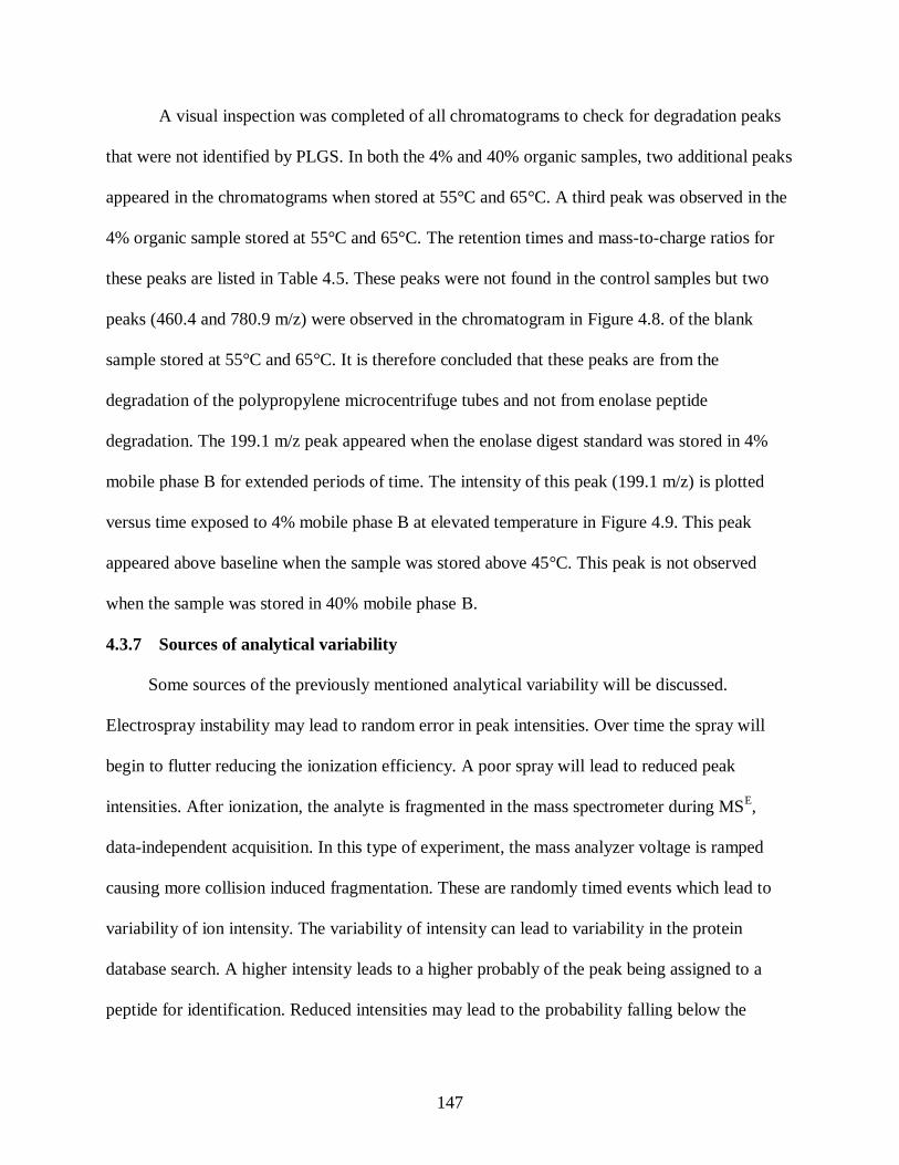
147
A visual inspection was completed of all chromatograms to check for degradation peaks
that were not identified by PLGS. In both the 4% and 40% organic samples, two additional peaks
appeared in the chromatograms when stored at 55°C and 65°C. A third peak was observed in the
4% organic sample stored at 55°C and 65°C. The retention times and mass-to-charge ratios for
these peaks are listed in Table 4.5. These peaks were not found in the control samples but two
peaks (460.4 and 780.9 m/z) were observed in the chromatogram in Figure 4.8. of the blank
sample stored at 55°C and 65°C. It is therefore concluded that these peaks are from the
degradation of the polypropylene microcentrifuge tubes and not from enolase peptide
degradation. The 199.1 m/z peak appeared when the enolase digest standard was stored in 4%
mobile phase B for extended periods of time. The intensity of this peak (199.1 m/z) is plotted
versus time exposed to 4% mobile phase B at elevated temperature in Figure 4.9. This peak
appeared above baseline when the sample was stored above 45°C. This peak is not observed
when the sample was stored in 40% mobile phase B.
4.3.7 Sources of analytical variability
Some sources of the previously mentioned analytical variability will be discussed.
Electrospray instability may lead to random error in peak intensities. Over time the spray will
begin to flutter reducing the ionization efficiency. A poor spray will lead to reduced peak
intensities. After ionization, the analyte is fragmented in the mass spectrometer during MSE,
data-independent acquisition. In this type of experiment, the mass analyzer voltage is ramped
causing more collision induced fragmentation. These are randomly timed events which lead to
variability of ion intensity. The variability of intensity can lead to variability in the protein
database search. A higher intensity leads to a higher probably of the peak being assigned to a
peptide for identification. Reduced intensities may lead to the probability falling below the

148
threshold necessary to confidently assign the peak to a peptide. Efforts were taken to reduce the
analytical variability but the results indicate that some is present.
4.4 Conclusion
Through the studies conducted in this Chapter, it is concluded that the exposure of peptides
to ultrahigh pressures, up to 45 kpsi, did not cause measurable degradation. Exposure to elevated
temperatures greater than 45°C in an acidic mobile phase environment for an excess of two hours
may cause sample degradation. For separations greater than two hours, the column temperature
should be no greater than 45°C. On-column degradation may occur at any temperature after 6
hours. These conclusions were made based on variability in peptide identifications and precursor
peak intensities in excess of that observed from analytical variability.
The implementation of elevated pressures and temperatures increases peak capacity
without increasing analysis time (Chapter 3). This research supports the use of elevated pressures
and temperatures for proteomics analysis but recommends that on-column time does not exceed
two hours for temperature greater than 45°C, or column temperature should not exceed 45°C for
separations longer than two hours. For targeted analyses, on-column analyte stability should be
reassessed.

149
4.5 TABLES
Pressure Temperature
Ambient Ambient (25°C)
Ambient 65°C
45 kpsi Ambient (25°C)
45 kpsi 65°C
Table 4.1. To assess the stability of peptides at elevated pressures and temperatures, the
MassPrep standard protein digest was storage for 10 hours at the conditions listed in this table.
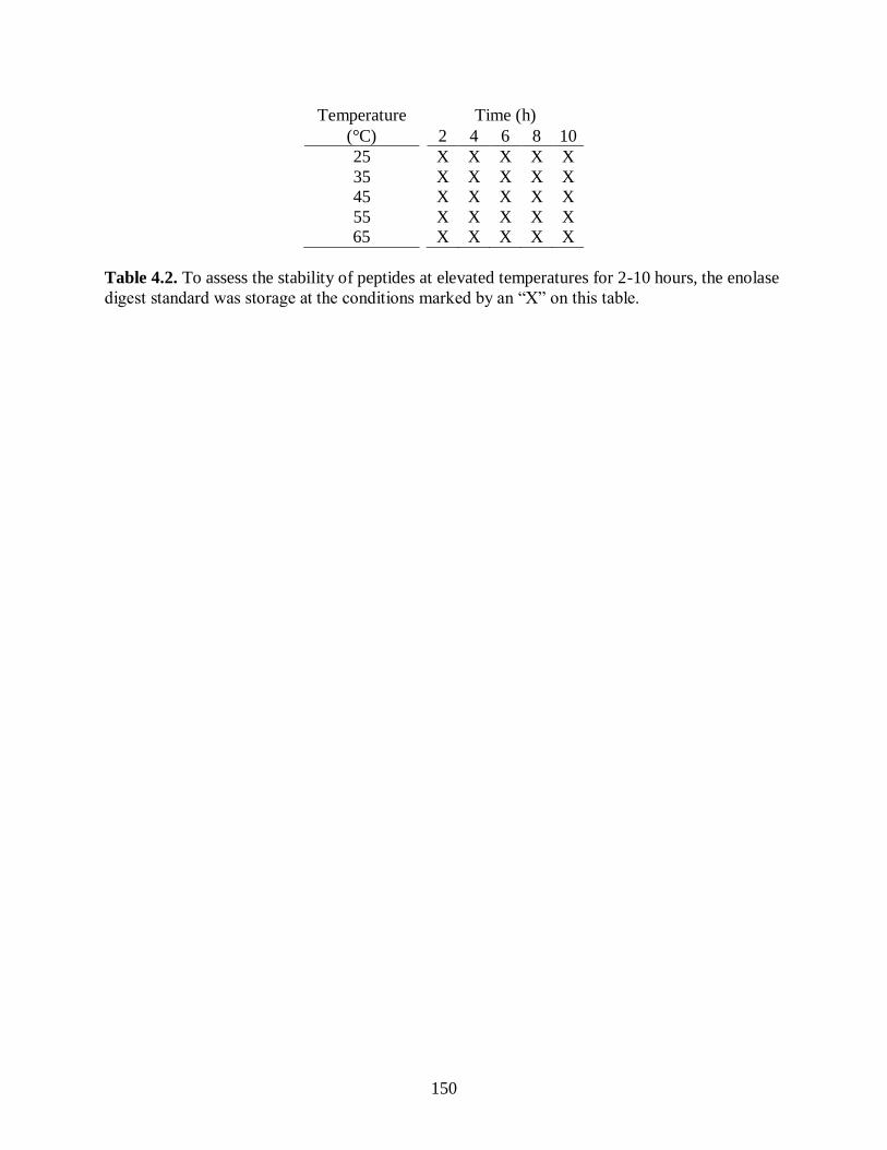
150
Temperature Time (h)
(°C) 2 4 6 8 10
25 X X X X X
35 X X X X X
45 X X X X X
55 X X X X X
65 X X X X X
Table 4.2. To assess the stability of peptides at elevated temperatures for 2-10 hours, the enolase
digest standard was storage at the conditions marked by an “X” on this table.

151
Temperature Time (h)
(°C) 2 4 6 8 10
25 0 3 1 4 7
35 1 1 0 4 6
45 2 1 0 3 6
55 2 0 0 0 7
65 1 1 2 0 2
Table 4.3. The number of significantly different peak intensities are listed for the enolase digest
sample stored in 4% mobile phase B at 25, 35, 45, 55, and 65°C for 2, 4, 6, 8, and 10 hours.
Intensities were compared to the unstressed, control sample A in which 19 peptide peaks were
identified. Most of the identified peptide peaks do not have significantly different intensities
when stored at any temperature for 6 hours. After 8 and 10 hours, many more peptides have
significantly different intensities. At these extreme conditions, about 6-7 peaks, or 35% of all
identifications, have significantly different intensities.
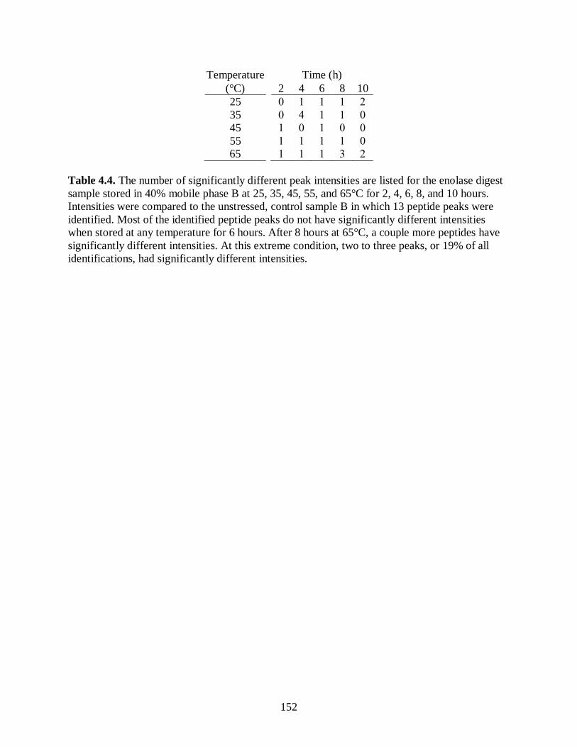
152
Temperature Time (h)
(°C) 2 4 6 8 10
25 1 1 1 2
35 4 1 1
45 1 1
55 1 1 1 1
65 1 1 1 3 2
Table 4.4. The number of significantly different peak intensities are listed for the enolase digest
sample stored in 40% mobile phase B at 25, 35, 45, 55, and 65°C for 2, 4, 6, 8, and 10 hours.
Intensities were compared to the unstressed, control sample B in which 13 peptide peaks were
identified. Most of the identified peptide peaks do not have significantly different intensities
when stored at any temperature for 6 hours. After 8 hours at 65°C, a couple more peptides have
significantly different intensities. At this extreme condition, two to three peaks, or 19% of all
identifications, had significantly different intensities.

153
Sample Retention Time (min) m/z
4% Mobile Phase B 28-31 199.1
4% and 40% Mobile Phase B 35.0 460.4
4% and 40% Mobile Phase B 36.2 780.9
Table 4.5. The retention times and mass-to-charge ratios (m/z) are listed for peaks that appeared
after the enolase digest was stored in the indicated sample solution. The 199.1 m/z peak appeared
when the enolase digest standard was stored in 4% mobile phase B for extended periods of time
above 45°C. This peak is not observed when the sample was stored in 40% mobile phase B. The
other two peaks were degradation products extracted from the polypropylene microcentrifuge
tubes used for sample storage.

154
4.6 FIGURES
a)
b)
Figure 4.1. The instrument diagram (a) shows the fluidic configuration for sample storage at
elevated pressures and temperatures. Part (b) shows the fluidic configuration for gradient/sample
loading and sample analysis. For gradient/sample loading, all valves were opened except the
nanoAcquity vent valve. For sample storage and analysis, all valves were closed except the
nanoAcquity vent valve. The haskel pump and column heater were regulated to the desired
pressure and temperature to stress the sample. During analysis, the haskel pump and column
heater were regulated to 15 kpsi and 30°C.

155
Figure 4.2. These chromatograms were from the analysis of the standard protein digest stored in the gradient storage loop. Storage
conditions are listed above each chromatogram.
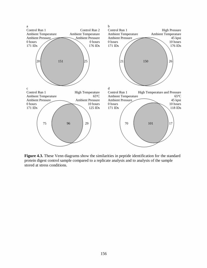
156
a
Control Run 1 Control Run 2
Ambient Temperature Ambient Temperature
Ambient Pressure Ambient Pressure
0 hours 0 hours
171 IDs 176 IDs
20 151 25
b
Control Run 1 High Pressure
Ambient Temperature Ambient Temperature
Ambient Pressure 45 kpsi
0 hours 10 hours
171 IDs 176 IDs
21 150 26
c
Control Run 1 High Temperature
Ambient Temperature 65ºC
Ambient Pressure Ambient Pressure 0 hours 10 hours
171 IDs 125 IDs
75 96 29
d
Control Run 1 High Temperature and Pressure
Ambient Temperature 65ºC
Ambient Pressure 45 kpsi 0 hours 10 hours
171 IDs 118 IDs
70 101 17
Figure 4.3. These Venn diagrams show the similarities in peptide identification for the standard
protein digest control sample compared to a replicate analysis and to analysis of the sample
stored at stress conditions.

157
Figure 4.4. The log peptide intensities are plotted comparing two replicate analyses of the
control standard protein digest. The confidence lines drawn on the graph are used to describe the
scatter from the dashed y=x line due to analytical variability. The formulas for each line and the
percent of data points contained within each set of lines are listed in the legend.

158
Figure 4.5. The log peptide intensities are plotted for the standard protein digest stored at 45 kpsi
and ambient temperature for 10 hours compared to the control. As listed in the legend, 95.2% of
the data points are contained within the green lines. This percentage is greater than that expected
due to analytical variability which indicates no change in peptide intensity from storage at
45 kpsi for 10 hours.

159
Figure 4.6. The log peptide intensities are plotted for the standard protein digest stored at 65°C
and ambient pressure for 10 hours compared to the control. As listed in the legend, 91.5% of the
data points are contained within the green lines. This percentage is less than that expected due to
analytical variability. Most of the variability occurs from data points falling below the y=x
dashed line which indicates a decrease of intensity for peptides in the elevated temperature
sample.

160
Figure 4.7. The log peptide intensities are plotted for the standard protein digest stored at 65°C
and 45 kpsi for 10 hours compared to the control. As listed in the legend, 88.8% of the data
points are contained within the green lines. This percentage is less than that expected due to
analytical variability. Most of the variability occurs from data points falling below the y=x
dashed line which indicates a decrease of intensity for peptides in the stressed sample.

161
Figure 4.8. These red and blue chromatograms are from the analysis of the enolase digest
control and stress sample stored at 65°C for 10 hours. Feature A (199.1 m/z) is a degradation
peak that appeared when enolase was stored in 4% mobile phase B at elevated temperatures. The
green chromatogram of mobile phase stored in the polypropylene microcentrifuge tubes at 65°C
for 10 hours shows that peak B (460.4 m/z) and peak C (780.9 m/z) were extracted from the tube
and are not peptide degradation products.

162
Figure 4.9. The intensity is plotted versus storage time for a degradation peak (199.1 m/z) that
appeared when the enolase digest standard was stored in 4% mobile phase B for extended
periods of time. This peak appeared when the sample was stored above 45°C. This peak is not
observed when the sample was stored in 40% mobile phase B.

163
4.7 REFERENCES
1. Zhang, X.; Fang, A.; Riley, C. P.; Wang, M.; Regnier, F. E.; Buck, C., Multi-dimensional
liquid chromatography in proteomics—A review. Analytica Chimica Acta 2010, 664 (2),
101-113.
2. Baker, E.; Liu, T.; Petyuk, V.; Burnum-Johnson, K.; Ibrahim, Y.; Anderson, G.; Smith,
R., Mass spectrometry for translational proteomics: progress and clinical implications.
Genome Med 2012, 4 (8), 1-11.
3. Meissner, F.; Mann, M., Quantitative shotgun proteomics: considerations for a high-
quality workflow in immunology. Nat. Immunol. 2014, 15 (Copyright (C) 2014 American
Chemical Society (ACS). All Rights Reserved.), 112-117.
4. Xie, F.; Smith, R. D.; Shen, Y., Advanced proteomic liquid chromatography. Journal of
Chromatography A 2012, 1261 (0), 78-90.
5. Cox, J.; Mann, M., Quantitative, High-Resolution Proteomics for Data-Driven Systems
Biology. Annual Review of Biochemistry 2011, 80 (1), 273-299.
6. Manning, M.; Patel, K.; Borchardt, R., Stability of Protein Pharmaceuticals. Pharm Res
1989, 6 (11), 903-918.
7. Kikwai, L.; Babu, R. J.; Kanikkannan, N.; Singh, M., Stability and degradation profiles
of Spantide II in aqueous solutions. European Journal of Pharmaceutical Sciences 2006,
27 (2–3), 158-166.
8. Smith, R. M.; Hansen, D. E., The pH-Rate Profile for the Hydrolysis of a Peptide Bond.
Journal of the American Chemical Society 1998, 120 (35), 8910-8913.
9. Wiśniewski, J. .; Zougman, A.; Mann, M., Nε-Formylation of lysine is a widespread
post-translational modification of nuclear proteins occurring at residues involved in
regulation of chromatin function. Nucleic Acids Research 2008, 36 (2), 570-577.
10. Patel, K.; Borchardt, R., Chemical Pathways of Peptide Degradation. II. Kinetics of
Deamidation of an Asparaginyl Residue in a Model Hexapeptide. Pharm Res 1990, 7 (7),
703-711.
11. Ji, J. A.; Zhang, B.; Cheng, W.; Wang, Y. J., Methionine, tryptophan, and histidine
oxidation in a model protein, PTH: Mechanisms and stabilization. Journal of
Pharmaceutical Sciences 2009, 98 (12), 4485-4500.
12. Patel, K.; Borchardt, R., Chemical Pathways of Peptide Degradation. III. Effect of
Primary Sequence on the Pathways of Deamidation of Asparaginyl Residues in
Hexapeptides. Pharm Res 1990, 7 (8), 787-793.
13. Bhatt, N.; Patel, K.; Borchardt, R., Chemical Pathways of Peptide Degradation. I.
Deamidation of Adrenocorticotropic Hormone. Pharm Res 1990, 7 (6), 593-599.
164
14. Neue, U. D., HPLC Columns: Theory, Technology, and Practice. Wiley: 1997.
15. Alzate, O., Neuroproteomics. Taylor & Francis: 2010.
16. Geiger, T.; Clarke, S., Deamidation, isomerization, and racemization at asparaginyl and
aspartyl residues in peptides. Succinimide-linked reactions that contribute to protein
degradation. Journal of Biological Chemistry 1987, 262 (2), 785-794.
17. Yang, H.; Zubarev, R. A., Mass spectrometric analysis of asparagine deamidation and
aspartate isomerization in polypeptides. ELECTROPHORESIS 2010, 31 (11), 1764-1772.
18. Srikanth, R.; Wilson, J.; Vachet, R. W., Correct identification of oxidized histidine
residues using electron-transfer dissociation. Journal of Mass Spectrometry 2009, 44 (5),
755-762.
19. Dell'Ova, V. E.; Denton, M. B.; Burke, M. F., Ultrasonic degasser for use in liquid
chromatography. Analytical Chemistry 1974, 46 (9), 1365-1366.
20. Ende, M.; Spiteller, G., Contaminants in mass spectrometry. Mass Spectrometry Reviews
1982, 1 (1), 29-62.
21. Chumsae, C.; Gaza-Bulseco, G.; Sun, J.; Liu, H., Comparison of methionine oxidation in
thermal stability and chemically stressed samples of a fully human monoclonal antibody.
Journal of Chromatography B 2007, 850 (1–2), 285-294.
22. Davies, M. J., The oxidative environment and protein damage. Biochimica et Biophysica
Acta (BBA) - Proteins and Proteomics 2005, 1703 (2), 93-109.

165
CHAPTER 5. Prefractionation Frequency Study with a 32 kpsi UHPLC for the
Multidimensional Separation of the Saccharomyces cerevisiae Proteome
5.1 Introduction
Studying the proteome gives understanding to the biological pathways that are occurring in
the cell.1,2,3
Due to the large number of protein encoding genes (6000 for S. cerevisiae),4
separation of the components in a biological mixture is required before analysis.5 There is no
single dimension separation with the peak capacity necessary to completely resolve all the
components of a cell lysate.6 Multidimensional separations have commonly been used to provide
more peak capacity.7,8
According to Giddings, the peak capacity of a multidimensional
separation is the multiplicative product of the peak capacities of the individual separations if the
separations are orthogonal and resolution is not lost in coupling the separations.9 For resolution
to be preserved, the second dimension would have to be faster than practically possible in liquid
chromatography (LC), or the first dimension would have to be extremely slowed down.
Therefore, fractionation of the first dimension is often necessary when coupling two columns.
The peak capacity of the first dimension then becomes the number of fractions. In order to
reduce the loss of peak capacity caused by fractionation, the second dimension should have the
greater peak capacity of the two separations.10,11
5.1.1 Prefractionation frequency
The peak capacity of the first dimension separation could be increased by taking more
fractions. However, higher prefractionation frequencies increase the analysis time and increase
the probability of splitting a peak across multiple fractions.12
Peak splitting dilutes the analyte

166
and lowers the limit of detection.13
From the study of prefractionation frequency in Chapter 2,
we learned that protein identifications plateaued when 20 or more fractions were taken.
5.1.2 Separations at elevated pressures and temperatures
Therefore, it is necessary to pursue solutions for increasing the peak capacity of the
second dimension. For liquid chromatography, ultrahigh performance LC (UPLC) has enabled
the use of microcapillary columns with sub-2 micron particles which have greater peak capacity
than standard bore columns.14
However, the pressure capabilities of the pump on a standard
UPLC limit the dimensions of commercial columns resulting in a maximum peak capacity of 200
in 90 minutes. In Chapter 3, new LC instrumentation with a constant pressure, high temperature
approach for peptide separations was introduced. The system modified a standard UPLC with a
pneumatic amplifier through a configuration of tubing and valves for separations up to
45000 psi. For a peptide analysis, the modified UHPLC, coupled to a qTOF Premier, produced a
peak capacity of 500 in 90 minutes on a meter-long microcapillary column packed with sub-2
micron particles. Peak capacity plateaued above 800 in 12 hours. Several columns of varying
lengths, packed with particles ranging from 1.1-1. μm, were characterized on the modified
UHPLC. For faster analysis, higher peak capacities and protein identifications were realized
when running an aggressive gradient on a long column with 1. μm particles than a shallower
gradient on a shorter column with smaller particles. The peak capacities produced with the
modified UHPLC were greater than that previously reported in the literature.15,16
Separations at higher temperatures reduce the viscosity of the mobile phase. Therefore,
longer columns can be used without reducing flow rate and increasing analysis time at a given
pressure. The higher temperatures also reduce the change in mobile phase viscosity throughout
the gradient on a constant pressure system.17,18,19
The resistance to mass transfer is reduced at

167
high temperatures which flattens the C-term portion of a Van Deemter plot and consequently
shifts optimal velocity to a higher value.20
The stability of the analyte, exposed to elevated
pressure and temperatures, was assessed in Chapter 4. Exposure of peptides to ultrahigh
pressures, up to 45 kpsi, did not show evidence of degradation. Peptide stability in acidic
reversed-phase LC solvents was confirmed for up to 2 hours at 65°C and for up to six hours at
45°C.
5.1.3 Orthogonality through prefractionation
For proteomics separations, benefits of the top-down (protein) and bottom-up (peptide)
strategies are often debated.21
Commonly, proteins are digested into peptides prior to analysis to
increase the solubility of the analyte.22
However, the sample is now more complex because there
are numerous peptides for each protein.23
Also, an inference problem occurs with the rebuilding
of a protein from the spectral data.24
The same peptide sequence may exist in two different
proteins, and it is difficult to determine to which protein the peptide should be assigned. Even
with these challenges, the bottom-up approach is more commonly practiced due to the greater
solubility of protein digests.25
More recently, a prefractionation approach has been implemented in which the intact
proteins are fractionated by the first dimension separation, and fractions are enzymatically
digested prior to analysis by LC-MS.26,27
Experimentally, prefractionation methods are more
orthogonal than other multidimensional separations because the sample is completely changed
via digestion between separations.28
Digestion, most commonly by trypsin, between the
separations enables the use of reversed-phase columns in both dimensions which tend to have
higher peak capacity than other LC separation modes such as ion exchange and size exclusion
chromatography.29
As opposed to bottom-up 2DLC experiments where peptides from a single

168
protein may be spread over the entire chromatogram, peptides from a single protein are confined
to a single fraction easing computational requirements. This may reduce the protein inference
problem in which a single peptide may be mistakenly assigned to multiple proteins.24
5.1.4 Equal-mass prefractionation
The practical 2D peak capacity increases if each fraction contains the same amount of
protein. The summed absorbance from the first dimension chromatogram is an appropriate guide
for determining equal-mass prefractionation (Chapter 2). The efficiency of the digestion can also
be increased with equal-mass fractionation as shown in this chapter. For most prefractionation
experiments, the enzyme to protein ratio is determined by assuming that the total protein loaded
onto the first dimension column was evenly distributed amongst the fractions.28
If there is excess
enzyme, autolysis of trypsin will occur.30
Peaks from trypsin peptides dominate the second
dimension chromatograms for these fractions (Chapter 2). A low enzyme to protein ratio
increases the probability that proteins are not fully digested.31
A poor digestion leads to poor
amino acid sequence coverage of the protein and the inability to detect the protein.23
The scope of this chapter was to couple prefractionation by equal-mass with the modified
UHPLC for the analysis of a model proteome, S. cerevisiae (Baker’s yeast). The effect of
prefractionation frequency on proteome coverage was assessed. The results were compared to
separations, of equal-mass fractions, on a standard UPLC as studied in Chapter 2. By
incorporating the modified UHPLC into the 2D experiment, the number of protein identifications
and percent sequence coverage increased as compared to the results in Chapter 2. The
improvement was realized with a lower prefractionation frequency and 2D separation time.
169
5.2 Materials and method
5.2.1 Materials
Water, acetonitrile, isopropyl alcohol and ammonium hydroxide were purchased from
Fisher Scientific (Fair Lawn, NJ). Ammonium acetate, ammonium bicarbonate, formic acid,
trifluoroacetic acid and iodoacetamide were purchased from Sigma-Aldrich Co. (St. Louis, MO).
RapigestTM
SF acid-labile surfactant and bovine serum album (BSA) digest standard were
obtained from Waters Corporation (Milford, MA). Dithiothreitol was purchased from Research
Products International. Water and acetonitrile were Optima LC-MS grade, and all other
chemicals were ACS reagent grade or higher. The harvest and lysis of the S. cerevisiae on
glycerol was previously described in Chapter 2.
5.2.2 Intact protein prefractionation
The prefractionation of intact proteins, as outlined in Figure 5.1., was performed on a
4.6 x 250 mm PLRP-S column with 5 µm particles, 300 Å (Agilent, Santa Clara, CA) heated to
80 °C. Four milligrams of total protein were injected onto the column. The mobile phase
composition and gradient profile is shown in Table 5.1. The separation was followed by UV
spectrophotometry to give a qualitative chromatogram. The wavelength was set to 214 nm,
which is the lambda max of the peptide bond.32
One-minute wide fractions were collected in
microcentrifuge tubes, lyophilized and stored at 80°C until further analysis.
5.2.3 Equal-mass fractionation
Each absorbance value for the UV chromatogram was summed with all previous
absorbance values from 10 to 48 minutes which corresponded to the time after the injection plug
and before the wash as follows
Summed Absorbance (ΣA) ∑ At
td tg
td (5-1)

170
where A = absorbance, t = time, td = dead time, and tg = gradient time.
The ΣA was normalized and plotted versus the first dimension separation time in Figure
5.2.a. The y-axis was annotated with hash marks in increments 0.05 which split the axis into 20
even parts. Lines were drawn from the hash marks on the y-axis to the corresponding x-
coordinate on the normalized ΣA curve. These x-coordinates were used to determine size of the
first dimension fractions. Each lyophilized one-minute-wide fraction (described in section 5.2.2.)
was reconstituted in 25 µL of 50 mM ammonium bicarbonate, pH 8. Three microliters of 6.67%
(w/v) api est™ SF in buffer were added. Solutions were vortexed, sonicated for 15 minutes,
and incubated at 80 ºC for 15 minutes to denature the proteins. The solutions were distributed
into 20 equal-mass fractions, as outlined in Table 5.2.
5.2.4 Protein digestion
The digestion is more efficient when carried out in a minimal amount of solvent.
Therefore, the 20 equal-mass fractions were lyophilized and reconstituted in 25 µL of 50 mM
ammonium bicarbonate. Three microliters of 6.67% (w/v) RapiGest™ SF in buffer were added.
Solutions were vortexed, sonicated for 15 minutes, and incubated at 80 ºC for 15 minutes to
denature the proteins. The proteins were reduced by adding 1 µL of 100 mM dithiothreitol,
vortexed, sonicated for 5 minutes, and incubated for 30 min at 60ºC. Proteins were then alkylated
with 1 µL of 200 mM iodoacetamide, vortexed, sonicated for 5 minutes, and stored protected
from light for 30 min at room temperature. The proteins were then digested by adding 10 µL of
667 ng/µL TPCK-modified trypsin in 50 mM ammonium bicarbonate (overnight, 37ºC). The
trypsin concentration was approximated to be a 50:1 (w/w) protein to enzyme ratio if the initial
protein amount was equally distributed across the 20 fractions. The digestion was quenched and
the api est™ SF was degraded using 44 µL 8:1:1 (v:v:v) water:acetonitrile:trifluoroacetic
171
acid (45 min, 37ºC). The fractions were centrifuged for 10 minutes at 14,000 Xg to pellet the
hydrolyzed surfactant, after which they were ready for analysis. The samples were transferred to
LC vials and spiked with 1.3 µL of a 1 pmol/L internal standard BSA digest (Waters).
To form the set of 10 fractions, 20 µL of neighboring pairs of fractions from the set of 20
was combined, lyophilized, and reconstituted with 10 µL 50 mM ammonium bicarbonate and 10
µL 98:1:1 (v:v:v) water:acetonitrile:trifluoroacetic acid. Likewise, the set of 5 fractions was
formed by combining 20 µL of every 4 consecutive fractions from the set of 20, lyophilizing,
and reconstituting with 10 µL 50 mM ammonium bicarbonate and 10 µL 98:1:1 (v:v:v)
water:acetonitrile:trifluoroacetic acid. All fractionation schemes are outlined in Table 5.2 and
depicted in Figure 5.2.
5.2.5 Peptide analysis by UHPLC-MS/MS
Each fraction was analyzed in duplicate by capillary RPLC-MS/MS using the UHPLC
system described in Chapter 3 coupled to a QTOF Premier MS. Mobile phase A was Optima
Grade water with 0.1% formic acid (Fisher), and mobile phase B was Optima-grade acetonitrile
with 0.1% formic acid (Fisher). Two microliters of the sample were pre-concentrated at the head
of a 110 cm x 75 µm, 1.9 µm BEH C18 column with 0.5% mobile phase B, and then separated
with a 25 µL gradient from 4-40%B followed by a wash at 85%B and equilibration at initial
conditions (Table 5.3). The column was run at 32 kpsi and 65°C to produce a 300 nL/min flow
rate. The outlet of the RPLC column was connected via a 30 cm x 20 µm ID piece of fused silica
capillary to an uncoated fused silica nanospray emitter with a 20 µm ID and pulled to a 10 µm
tip (New Objective, Woburn, MA) operated at 2.6 kV. Data-independent acquisition, or MSE
scans, was performed with the instrument set to acquire parent ion scans from m/z 50-1990 over

172
0.6 sec at 5.0 V. The collision energy was then ramped from 15-40 V over 0.6 sec with 0.1 sec
interscan delay.
5.2.6 Peptide data processing
The peptide LC-MS/MS data were processed using ProteinLynx Global Server 2.5
(Waters). The MSE spectra were searched against a database of known yeast proteins from the
Uni-Prot protein knowledgebase ( www.uniprot.org) with a reversed sequence appended to the
end. The false discovery rate was set to 100% to yield data compatible for further processing.
After the database search was complete, the results were imported into Scaffold 4.2.0
(Proteome Software, Portland, OR). The minimum protein probability and peptide probability
filters were set to a 5% false discovery rate, and the minimum number of peptides required for
protein identification was set to 3. Peptides matching multiple proteins were exclusively assigned
to the protein with the most evidence. The spectral counts for each peptide assigned to a protein
were summed to give the quantitative value of that protein. The value was normalized by
multiplying the average total number of spectra, for all yeast samples grown on the same media,
divided by the individual sample’s total number of spectra.33,34
5.3 Discussion
5.3.1 Protein identifications
By combining the prefractionation techniques studied in Chapter 2 with the new UHPLC
developed in Chapter 3, the return on protein identifications per unit time was greatly increased.
In Figure 5.3, the number of protein identifications versus number of fractions is plotted for each
prefractionation experiment. The number of fractions is proportional to the separation time as
each fraction had a 1.5 hour retention window. The red line shows the improvement for equal-
mass fractionation versus equal-time fractionation (blue line) as was discussed in Chapter 2. The

173
green line demonstrates the improvement in protein identifications when UHPLC with a 110 cm
long column was employed for the second dimension separation. The set of 5 fractions analyzed
on the long column identified 472 proteins which exceeded the number of proteins identified by
the analysis on the standard system even with increased first dimension fractionation. When first
dimension sampling was increased to 10 fractions, 701 proteins were identified. The number of
identifications leveled off at 20 fractions with 776 protein identifications. With the ability to
operate at higher pressures, the peak capacity gained through the use of a longer column resulted
in the identification of more proteins with less first dimension fractions and less total separation
time.
5.3.2 Analysis time
To make a fair comparison between the standard UPLC and modified UHPLC system,
the second dimension separation times had to be similar. This was somewhat difficult as the
standard system is programmed with a gradient time and constant flow rate whereas the modified
system is programmed with a gradient volume and constant pressure. The gradient volume was
25 μL, and modified UHPLC was pressured to 32 kpsi. The measured flow rate was 3 nL/min
at 65°C and 4% mobile phase B. Because mobile phase composition was changing throughout
the run, the flow rate was also changing slightly but theoretically by less than 5% as previously
explained.17,18,19
Peaks eluted for 100 minutes as evident by the chromatograms in Figure 5.4.
Though the separation window was similar for the separation on the modified UHPLC
and standard UPLC, the total run time for the separations on the modified system was longer.
The standard system had a trap column to preconcentrate the sample and ultimately reduce the
injection time. Addition of a trap column to the modified system resulted in band broadening
which was suspected to occur from mixing in the nano-tee between the trap and analytical

174
column. In the future, the modified system should be engineered to have a total run time more
comparable to the standard system.
5.3.3 Increased peptide peak intensity
Another observation from the 2D chromatograms in Figure 5.4. is that peak intensities
are much greater with the modified UHPLC. Chapter 3 demonstrated that through the use of long
columns and elevated pressures, narrower peak widths could be achieved as compared to a
separation with the standard system. The peptides were focused into narrow peaks which
contributed to the higher intensity. With increased intensity, more peptide peaks were above the
limit of detection which contributed to the increase in protein identifications with the modified
UHPLC system.
5.3.4 Protein identifications per fractions
To further discuss the number of protein identifications achieved with the modified
UHPLC, the number of proteins identified per fraction is plotted in Figure 5.5. for each
prefractionation frequency. The light gray bars show the total protein identifications in each
fraction, and the dark gray bars signify the unique protein identifications in each fraction. The
total protein count was defined as any protein found within a given fraction; thus, if a protein
were to be found in multiple fractions it would be counted in each fraction. The unique protein
values count each protein entry only once. Proteins identified in multiple fractions were assigned
to the fraction in which it was most intense. Though there were few peaks during the beginning
and end of the first dimension chromatogram, as evident from the overlaid red trace, proteins
were still identified in the analysis of the peptide digests of these fractions. On average, more
unique proteins were identified per fraction as prefractionation frequency decreased but total
proteins identifications per fraction remained constant.

175
To compare the number of proteins identified per fraction with the modified UHPLC to
that run on the standard system, Figure 5.6, Figure 5.7 and Figure 5.8 should be considered for
20, 10 and 5 fractions, respectively. In each figure, part (a) shows the protein identifications per
fraction using the long column at elevated pressures while part (b) shows data collected with the
standard system. At every fractionation frequency, more proteins were identified per fraction
especially for the first fraction with the modified UHPLC. The increased peak capacity from
using the long column at elevated pressure contributed to the increase in protein identifications.
5.3.5 Protein digestion
As observed in Figures 5.5 – 5.7, there was a large increase in protein identifications in
fraction one when the second dimension analysis occurred at 32 kpsi. The increase in
identifications was greater for this particular fraction due to when the digestion occurred in the
experimental protocol and due to the incorporation of sonication after each step of the protocol.
For the samples run on the standard system, digestion occurred before the equal-time fractions
were combined into equal-mass fractions. For the samples run on the modified system, digestion
occurred after recombination into equal-mass fractions, and sonication was incorporated
throughout the digestion protocol. Combining the fractions based on first dimension separation
data, more evenly distributed the proteins amongst the fractions. Therefore, the enzyme to
protein ratio was more consistent for each fraction. With a better estimation of this ratio,
autolysis of the enzyme was less likely in fractions corresponding to less intense first dimension
peaks. Also, less protein remained undigested in the fractions containing large amounts of
protein. Sonication aided in the denaturing of proteins which facilitated the delivery of enzyme
to the digestion sights. Digestion of equal-mass fractions is recommended for future
prefractionation experiments.

176
5.3.6 Protein molecular weight distribution
The molecular weight distributions of identified proteins are displayed in in Figure 5.9a
for the separations at 32 kpsi and Figure 5.9b for the separations at 8 kpsi. The molecular weight
distribution corresponding to the 5, 10 and 20 fractions are portrayed by the black, gray and
white bars, respectively. Proteins were identified with molecular weight s up to 250 kDa. For all
methods, the median molecular weight was 39-40 kDa which was similar to the literature value
of approximately 42.2 kDa for the S. cerevisiae proteome.35
For the fractions run at 32 kpsi, the
increase in identifications occurred mostly for lower molecular weight proteins, 20-70 kDa.
The molecular weight chromatograms in Figure 5.10 for 20 (parts a,b), 10 (parts c,d), and
5 (parts e,f) first dimension fractions plot protein mass on the y-axis and first dimension fraction
on the x-axis. The log quantitative value for each protein is plotted as a gray-scale intensity in the
z-direction. The molecular weight chromatograms on the left (Figure 5.10 a,c,e) were from the
modified UHPLC at 32 kpsi with a 110 cm column, and the chromatograms on the right (Figure
5.10 b,d,f) were from the standard UPLC at 8 kpsi with a 25 cm commercial column. The
correlation between protein molecular weight and first dimension fraction was stronger for the
separations at 32 kpsi. In other words, the later fractions contained proteins with larger molecular
weights. Larger proteins would have more sites to interact with the stationary phase causing
them to elute later in the first dimension fractions. Though the first dimension separation method
was the same for all experiments, the separations at 8 kpsi and 32 kpsi were completed with two
different first dimension prefractionation sets due to limited sample volume. The differences in
the mass chromatograms may also be due to the changes the digestion protocol as explained in
the previous section.

177
5.3.7 Venn diagram comparisons
Analysis on the long column at elevated pressures resulted in a greater than two fold-
change in protein identifications as compared to the standard system for the analysis of 5 and 10
fractions as seen in Figure 5.11. (a and b). About 90% of the proteins identified with the standard
system were also identified by analysis on the modified UHPLC. When first dimension sampling
increased to 20 fractions, the improvement between analysis on the modified and standard
UHPLC systems decreased to 79% more identifications. An 84% overlap in identifications was
observed for the 20 fractions run on both systems. The increased fractionation frequency may
cause proteins to be split amongst multiple fractions resulting in the slightly lower improvement
for this data set.
In Figure 5.12, the overlap in protein identifications was compared for 5, 10 and 20 first
dimension fractions analyzed by the modified UHPLC-MS. When fractionation was doubled
from 5 to 10, 198 additional proteins were identified, and 46 protein identifications were lost for
a net increase of 27%. Another doubling of fractionation from 10 to 20, resulted in 212
additional protein identifications at a cost of 51 protein identifications for a net gain of 22%. The
total number of protein identifications in the Venn diagrams in Figure 5.11 and Figure 5.12
included every unique protein entry in the replicate analyses. The numbers were slightly larger
than the protein identifications in Figure 5.3 which corresponded to the average number
(arithmetic mean) of identifications between two replicate analyses. The Venn comparisons
further demonstrate that excessive prefractionation should be avoided to reduce peak splitting.
With the modified UHPLC and long microcapillary column, the peak capacity in the second
dimension is increased reducing the need for a high prefractionation frequency.
178
5.3.8 Fractions per protein
The first dimension chromatogram was crowded with many overlapping peaks making it
impractical to determine peak widths for individual proteins. As an alternative merit, fractions
per protein was defined as the number of fractions in which a single protein was identified. The
graph in Figure 5.13 shows the percentage of proteins identified in one, two and three-or-more
fractions for each prefractionation frequency. The majority of proteins were identified in only
one fraction. As fractionation frequency increased, more proteins were identified in multiple
fractions. These fractions may or may not be adjacent. When a protein was split between
multiple fractions, it was diluted which may cause it to fall below the limit of detection. When
comparing the fractions per protein for data collected with the modified and standard UHPLC, a
larger percentage of proteins were identified in multiple fractions with the modified system.
Since the first dimension separations were identical, there could not be increased protein peak
splitting or broadening. Also, blank runs after the second dimension separations did not show
evidence of carryover. The increased identification of proteins across multiple fractions was
most likely related to the increased peak intensities in the second dimension separation as
explained earlier and shown in Figure 5.4. Hypothetically, a protein peak split across two
fractions has the majority of the peak contained in fraction 1 and the tail of the peak contained in
fraction 2. When both fractions are digested and analyzed by LC-MS, the corresponding peptide
peaks would be more intense in fraction 1 than fraction 2 because most of the protein molecules
are contained in fraction 1. For fraction 2, the intensity of the peptide peaks run on the standard
system may fall below the limit of detection. With the peak intensity gained from the long
column run at elevated pressures, the protein could be identified in fraction 2 from its assigned
peptides.
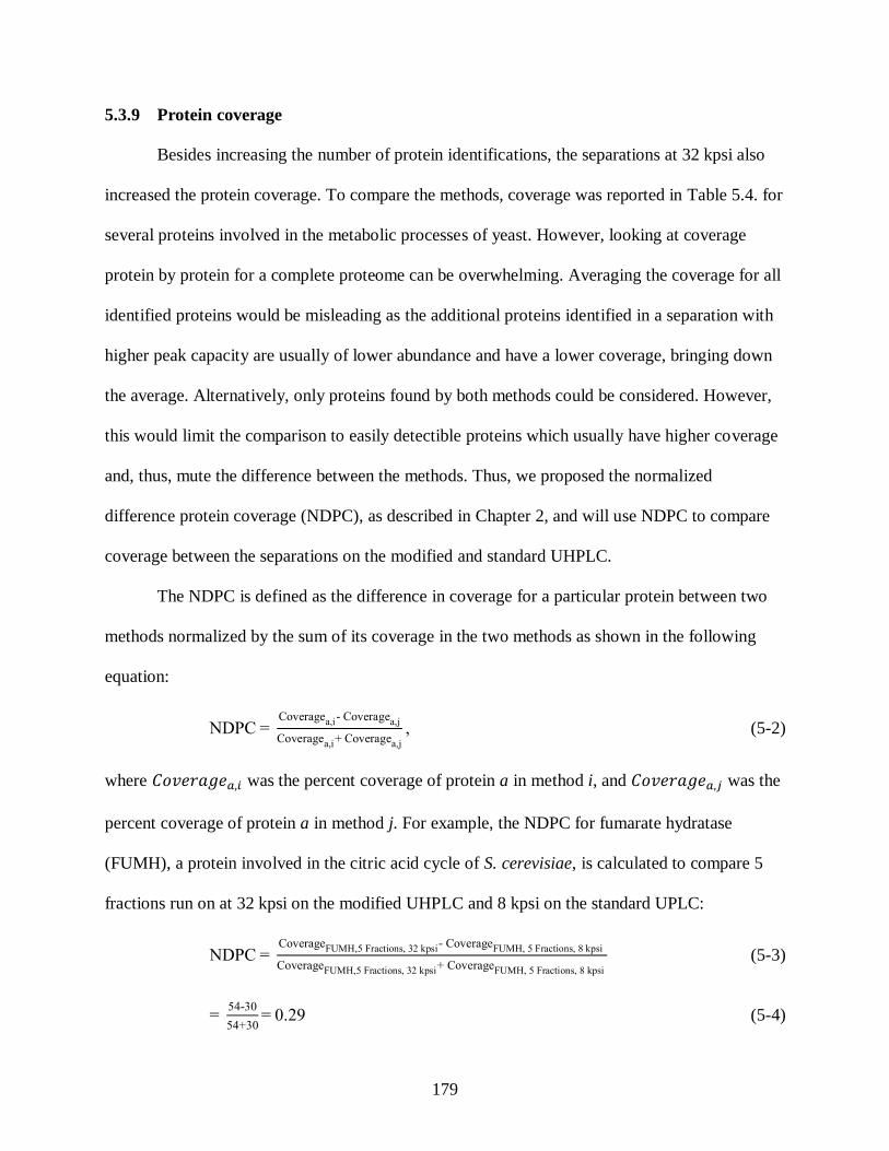
179
5.3.9 Protein coverage
Besides increasing the number of protein identifications, the separations at 32 kpsi also
increased the protein coverage. To compare the methods, coverage was reported in Table 5.4. for
several proteins involved in the metabolic processes of yeast. However, looking at coverage
protein by protein for a complete proteome can be overwhelming. Averaging the coverage for all
identified proteins would be misleading as the additional proteins identified in a separation with
higher peak capacity are usually of lower abundance and have a lower coverage, bringing down
the average. Alternatively, only proteins found by both methods could be considered. However,
this would limit the comparison to easily detectible proteins which usually have higher coverage
and, thus, mute the difference between the methods. Thus, we proposed the normalized
difference protein coverage (NDPC), as described in Chapter 2, and will use NDPC to compare
coverage between the separations on the modified and standard UHPLC.
The NDPC is defined as the difference in coverage for a particular protein between two
methods normalized by the sum of its coverage in the two methods as shown in the following
equation:
NDPC Coveragea,i- Coveragea,
Coveragea,i Coveragea, , (5-2)
where was the percent coverage of protein a in method i, and was the
percent coverage of protein a in method j. For example, the NDPC for fumarate hydratase
(FUMH), a protein involved in the citric acid cycle of S. cerevisiae, is calculated to compare 5
fractions run on at 32 kpsi on the modified UHPLC and 8 kpsi on the standard UPLC:
NDPC CoverageFUMH,5 Fractions, 32 kpsi- CoverageFUMH, 5 Fractions, 8 kpsi
CoverageFUMH,5 Fractions, 32 kpsi CoverageFUMH, 5 Fractions, 8 kpsi
(5-3)
54-3
54 3 .2 (5-4)
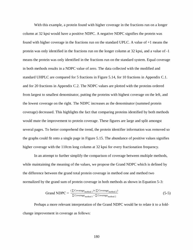
180
With this example, a protein found with higher coverage in the fractions run on a longer
column at 32 kpsi would have a positive NDPC. A negative NDPC signifies the protein was
found with higher coverage in the fractions run on the standard UPLC. A value of +1 means the
protein was only identified in the fractions run on the longer column at 32 kpsi, and a value of 1
means the protein was only identified in the fractions run on the standard system. Equal coverage
in both methods results in a NDPC value of zero. The data collected with the modified and
standard UHPLC are compared for 5 fractions in Figure 5.14, for 10 fractions in Appendix C.1.
and for 20 fractions in Appendix C.2. The NDPC values are plotted with the proteins ordered
from largest to smallest denominator, putting the proteins with highest coverage on the left, and
the lowest coverage on the right. The NDPC increases as the denominator (summed protein
coverage) decreased. This highlights the fact that comparing proteins identified by both methods
would mute the improvement to protein coverage. These figures are large and split amongst
several pages. To better comprehend the trend, the protein identifier information was removed so
the graphs could fit onto a single page in Figure 5.15. The abundance of positive values signifies
higher coverage with the 110cm long column at 32 kpsi for every fractionation frequency.
In an attempt to further simplify the comparison of coverage between multiple methods,
while maintaining the meaning of the values, we propose the Grand NDPC which is defined by
the difference between the grand total protein coverage in method one and method two
normalized by the grand sum of protein coverage in both methods as shown in Equation 5-3:
rand NDPC (∑Coverage
method 1)-(∑Coverage
method 2)
∑Coveragemethod 1
∑Coveragemethod 2
(5-5)
Perhaps a more relevant interpretation of the Grand NDPC would be to relate it to a fold-
change improvement in coverage as follows:

181
Fold-Change in Coverage ∑Coverage
method 1
∑Coveragemethod 2
1 rand NDPC
1- rand NDPC (5-6)
If the fold-change is less than one, the negative reciprocal of the value is used as is
conventional with fold-change calculations. The Grand NDPC and Fold-Change in Coverage is
listed in Table 5.5. Positive values represent higher coverage with the 110 cm long column at 32
kpsi. For each prefractionation frequency, a greater than two-fold change in protein coverage
was observed when the second dimension separation occurred on the 110cm long column at 32
kpsi as opposed to the 25 cm commercial column at 8 kpsi.
5.4 Conclusions
A challenge in proteomics has always been to obtain more information from the sample
without increasing the analysis time. By using S. cerevisiae lysate as a model proteome for a
prefractionation type multidimensional separation, the effects of prefractionation frequency and
second dimension peak capacity on protein identifications were investigated. The gained peak
capacity from performing the second dimension separation on a long column at 32 kpsi yielded
an increase in protein identifications and approximately doubled the amino acid sequence
coverage compared to separations on a standard system. With five first dimension fractions, the
modified UHPLC identified 472 proteins while only 171 proteins were identified with the
standard UPLC. It took 20 fractions, which quadrupled the separation time, to yield a maximum
of 456 fractions with the standard UPLC. Identifications reached 776 proteins with 20 fractions
run on the modified UHPLC. The instrumentation and methods described in this chapter will
enable completion of differential proteomics studies in a shorter amount of time and produce
more information about the samples.

182
5.5 TABLES
Time
(min)
Flow Rate
(mL/min)
90:5:5
H2O:ACN:IPA +
0.2% TFA
(%A)
50:50
ACN:IPA
+ 0.2% TFA
(%B)
0 1.0 100 0
2 1.0 100 0
5 1.0 75 25
40 1.0 50 50
45 1.0 35 65
45.1 1.0 0 100
50 1.0 0 100
50.1 1.0 100 0
Table 5.1. Chromatographic conditions for the reversed-phase prefractionation of intact proteins.
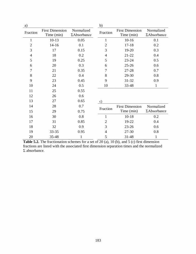
183
a) b)
Fraction First Dimension
Time (min)
Normalized
ΣAbsorbance
Fraction First Dimension
Time (min)
Normalized
ΣAbsorbance
1 10-13 0.05
1 10-16 0.1
2 14-16 0.1
2 17-18 0.2
3 17 0.15
3 19-20 0.3
4 18 0.2
4 21-22 0.4
5 19 0.25
5 23-24 0.5
6 20 0.3
6 25-26 0.6
7 21 0.35
7 27-28 0.7
8 22 0.4
8 29-30 0.8
9 23 0.45
9 31-32 0.9
10 24 0.5
10 33-48 1
11 25 0.55
12 26 0.6
13 27 0.65
c)
14 28 0.7
Fraction
First Dimension
Time (min)
Normalized
ΣAbsorbance 15 29 0.75
16 30 0.8
1 10-18 0.2
17 31 0.85
2 19-22 0.4
18 32 0.9
3 23-26 0.6
19 33-35 0.95
4 27-30 0.8
20 35-48 1
5 31-48 1
Table 5.2. The fractionation schemes for a set of 20 (a), 10 (b), and 5 (c) first dimension
fractions are listed with the associated first dimension separation times and the normalized
Σ absorbance.
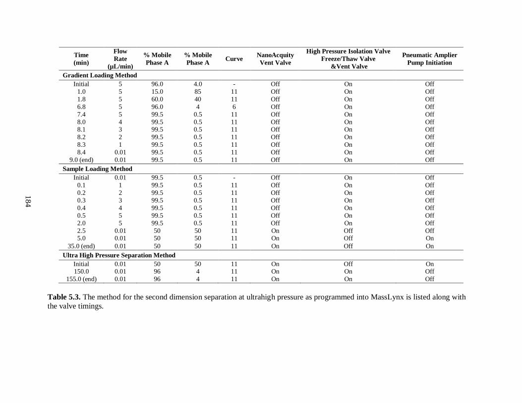
184
Time
(min)
Flow
Rate
(µL/min)
% Mobile
Phase A
% Mobile
Phase A Curve
NanoAcquity
Vent Valve
High Pressure Isolation Valve
Freeze/Thaw Valve
&Vent Valve
Pneumatic Amplier
Pump Initiation
Gradient Loading Method
Initial 5 96.0 4.0 - Off On Off
1.0 5 15.0 85 11 Off On Off 1.8 5 60.0 40 11 Off On Off 6.8 5 96.0 4 6 Off On Off 7.4 5 99.5 0.5 11 Off On Off 8.0 4 99.5 0.5 11 Off On Off 8.1 3 99.5 0.5 11 Off On Off 8.2 2 99.5 0.5 11 Off On Off 8.3 1 99.5 0.5 11 Off On Off 8.4 0.01 99.5 0.5 11 Off On Off
9.0 (end) 0.01 99.5 0.5 11 Off On Off
Sample Loading Method
Initial 0.01 99.5 0.5 - Off On Off
0.1 1 99.5 0.5 11 Off On Off 0.2 2 99.5 0.5 11 Off On Off 0.3 3 99.5 0.5 11 Off On Off 0.4 4 99.5 0.5 11 Off On Off 0.5 5 99.5 0.5 11 Off On Off 2.0 5 99.5 0.5 11 Off On Off 2.5 0.01 50 50 11 On Off Off 5.0 0.01 50 50 11 On Off On
35.0 (end) 0.01 50 50 11 On Off On
Ultra High Pressure Separation Method
Initial 0.01 50 50 11 On Off On 150.0 0.01 96 4 11 On On Off
155.0 (end) 0.01 96 4 11 On On Off
Table 5.3. The method for the second dimension separation at ultrahigh pressure as programmed into MassLynx is listed along with
the valve timings.

185
Protein Coverage (%)
Assigned Peptides
Name Entry
Shotgun 5 10 20
Shotgun 5 10 20
Isocitrate lyase ACEA
- 43 71 69
- 19 35 36
Aconitate hydratase ACON
20 65 53 69
13 53 54 72 Acetyl-coenzyme A synthetase 1 ACS1
33 63 46 64
18 53 63 69
Acetyl-coenzyme A synthetase 2 ACS2
- 10 10 20
- 2 4 8 Alcohol dehydrogenase 1 ADH1
56 74 73 74
11 26 29 29
Alcohol dehydrogenase 2 ADH2
68 76 79 77
26 42 45 47 Alcohol dehydrogenase 3 ADH3
- 35 55 65
- 10 16 20
Alcohol dehydrogenase 6 ADH6
- - 13 38
- - 3 11 Aldehyde dehydrogenase 2 ALDH2
- 39 50 61
- 15 19 26
Aldehyde dehydrogenase 3 ALDH3
- 9 19 20
- 2 3 3 K-activated aldehyde dehydrogenase ALDH4
75 88 83 85
37 53 63 66
Fructose-bisphosphate aldolase ALF
54 73 80 91
17 29 34 38 Citrate synthase CISY1
35 61 59 65
15 35 35 46
Succinate dehydrogenase DHSA
- 26 31 53
- 10 15 25 Dihydrolipoyl dehydrogenase DLDH
23 65 70 76
6 32 36 42
Enolase 1 ENO1
75 86 86 88
31 21 25 26 Enolase 2 ENO2
72 88 83 92
12 51 57 62
Fumarate reductase FRDS
- 42 55 60
- 18 22 30
Fumarate hydratase FUMH
- 54 61 57
- 24 28 31 Glyceraldehyde-3-P dehydrogenase 1 G3P1
83 92 85 92
14 45 28 32
Glyceraldehyde-3-P dehydrogenase 2 G3P2
88 91 85 91
6 10 10 13 Glyceraldehyde-3-P dehydrogenase 3 G3P3
92 92 96 94
35 24 49 52
Glucose-6-phosphate isomerase G6PI
44 62 69 68
21 37 45 50 Glycerol-3-phosphate dehydrogenase GPD1
- 65 63 59
- 24 27 27
Glycerol-3-phosphate dehydrogenase GPD2
- 11 32 26
- 2 8 9 Glycerol-3-phosphatase 2 GPP2
- - - 19
- - - 4
Hexokinase-1 HXKA
42 68 75 83
16 30 37 51 Hexokinase-2 HXKB
40 73 71 82
11 31 42 42
Glucokinase-1 HXKG
57 74 71 87
23 41 51 57 Isocitrate dehydrogenase 1 IDH1
11 59 59 65
3 23 22 24
Isocitrate dehydrogenase 2 IDH2
12 71 64 81
2 17 16 24 6-phosphofructokinase subunit α K6PF1
23 57 57 68
15 62 76 86
Pyruvate kinase 1 KPYK1
77 86 82 88
33 54 61 64 Malate synthase 1 MASY
- 48 48 57
- 26 22 38
Malate dehydrogenase, cyto MDHC
10 52 53 56
3 16 16 22 Malate dehydrogenase, mito MDHM
60 77 75 84
15 24 24 31
2-oxoglutarate dehydrogenase E1 ODO1
9 34 54 51
6 29 47 56 γ-glutamyl phosphate reductase ODO2
- 38 47 48
- 14 19 25
Pyruvate dehydrogenase E1 comp β ODPB
- 49 37 66
- 11 10 18 Phosphoenolpyruvate carboxykinase PCKA
44 72 83 74
19 48 54 59
Pyruvate decarboxylase isozyme 1 PDC1
62 69 65 71
30 40 45 53 Pyruvate decarboxylase isozyme 5 PDC5
- - 17 27
- - 5 13
Pyruvate decarboxylase isozyme 6 PDC6
- 19 28 37
- 5 11 19 Phosphoglycerate kinase PGK
87 90 83 93
38 54 57 61
Phosphoglycerate mutase 1 PMG1
84 83 90 80
22 26 29 31 Pyruvate carboxylase 1 PYC1
- 43 40 48
- 40 42 23
Pyruvate carboxylase 2 PYC2
- 34 34 44
- 10 9 52 Succinyl-CoA ligase subunit α SUCA
52 75 69 72
12 22 26 27
Succinyl-CoA ligase subunit β SUCB
19 49 59 72
7 31 37 40 Transaldolase 1 TAL1
24 62 62 81
6 17 35 41
Transaldolase 2 TAL2
- 65 41 61
- 21 15 25
Transketolase 1 TKT1
- 54 73 68
- 35 48 50 Transketolase 2 TKT2
- 32 42 48
- 16 24 29
Triosephosphate isomerase TPIS
71 90 93 88
15 28 28 31
Average
50 59 60 66
17 27 31 36
Table 5.4. For the separations on the modified UHPLC, the protein coverage (%) and number of
peptides used to identify each protein is reported for the some of the proteins involved in S.
cerevisiae metabolism

186
Fractions Grand NDPC Fold Change In Coverage
5 0.48 2.9
10 0.39 2.3
20 0.37 2.2
Table 5.5. The Grand NDPC and Fold-Change in Coverage are listed for each fractionation
frequency. Positive values represent higher coverage when the 110cm long column at 32 kpsi
was used for the second dimension separation as compared to the shorter column run on the
standard system. The Fold-Change in Coverage increased as fractionation frequency decreased.

187
5.6 FIGURES
Figure 5.1. The workflow for the prefractionation method started with HPLC-UV of the intact
proteins. Thirty-eight one-minute-wide fractions were collected, lyophilized, and pooled into
20 equal-mass fractions. The 20 equal-mass fractions were digested and also pooled into 10 and
5 equal-mass fractions. The set of 20, 10, and 5 equal-mass fractions were analyzed with a
second dimension separation by the modified UHPLC-MS at 32 kpsi. The spectral data were
searched against a genomic database to identify the proteins.

188
a) b)
c)
Figure 5.2. The normalized ΣAbsorbance trace is plotted versus the first dimension separation
time to determine the equal-mass prefractionation timings. The y-axis is equally divided into 20
(a), 10 (b), and 5 (c) fractions. A line is drawn from the Σ Absorbance trace to the x-axis to
determine when to take fractions from the first dimension. The UV chromatogram is overlaid on
these plots to show how the area under the peaks is relatively equal in every fraction.
1.00
0.75
0.50
0.25
0.00
No
rmal
ized
Σ A
bso
rban
ce
40302010
Time (min)
2.5
2.0
1.5
1.0
0.5
0.0
AU
(21
4 n
m)
1.0
0.8
0.6
0.4
0.2
0.0
No
rmal
ized
Σ A
bso
rban
ce
40302010
Time (min)
2.5
2.0
1.5
1.0
0.5
0.0
AU
(21
4 n
m)
1.0
0.8
0.6
0.4
0.2
0.0
No
rmal
ized
Σ A
bso
rban
ce
40302010
Time (min)
2.5
2.0
1.5
1.0
0.5
0.0
AU
(21
4 n
m)

189
Figure 5.3. The number of protein identifications is plotted versus number of first dimension
fractions. The green line is for the prefractionation experiment, described in this chapter, run on
the modified UHPLC at 32 kpsi. As a comparison, the results from this chapter where
superimposed on Figure 2.5 (red and blue traces) for a prefractionation study with a standard
UPLC. The number of protein identifications greatly increased through use of long columns on
the UHPLC.

190
a) Modified UHPLC b) Standard UPLC
c) d)
e) f)
Figure 5.4. Two-dimensional chromatograms for 20 (a,b), 10 (c,d), and 5 (e,f) first dimension
fractions are plotted with the first dimension (protein) fraction number versus the second
dimension (peptide) separation. Base peak intensity BPI is plotted in the z-direction.
Chromatograms on the left (a,c,e) are from the modified UHPLCat 32 kpsi with a 110 cm
column, and chromatograms on the right (b,d,f) are run on a standard UPLC at 8 kpsi with a
25 cm commercial column. The same amount of protein was loaded onto the column in both
analyses. The gain in intensity was due to the decreased peak widths on the longer column.
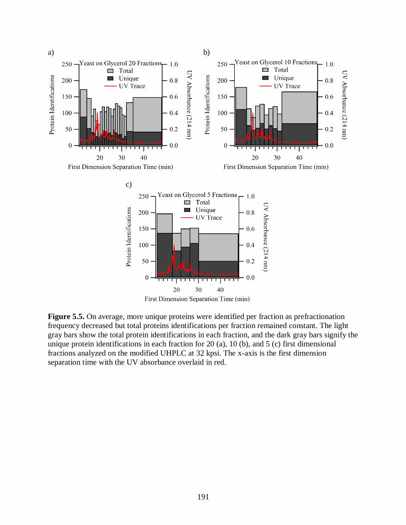
191
a) b)
c)
Figure 5.5. On average, more unique proteins were identified per fraction as prefractionation
frequency decreased but total proteins identifications per fraction remained constant. The light
gray bars show the total protein identifications in each fraction, and the dark gray bars signify the
unique protein identifications in each fraction for 20 (a), 10 (b), and 5 (c) first dimensional
fractions analyzed on the modified UHPLC at 32 kpsi. The x-axis is the first dimension
separation time with the UV absorbance overlaid in red.

192
a) Modified UHPLC b) Standard UPLC
Figure 5.6. More proteins were identified per fraction when the fractions were run on the 110 cm
column at 32 kpsi (a) as compared to the standard UPLC (b). The light gray bars show the total
protein identifications in each fraction, and the dark gray bars signify the unique protein
identifications in each fraction for 20 first dimension fractions.

193
a) Modified UHPLC b) Standard UPLC
Figure 5.7. More proteins were identified per fraction when the fractions were run on the 110 cm
column at 32 kpsi (a) as compared to the standard UPLC (b).The light gray bars show the total
protein identifications in each fraction, and the dark gray bars signify the unique protein
identifications in each fraction for 10 first dimension fractions.

194
a) Modified UHPLC b) Standard UPLC
Figure 5.8. More proteins were identified per fraction when the fractions were run on the 110 cm
column at 32 kpsi (a) as compared to the standard UPLC (b).The light gray bars show the total
protein identifications in each fraction, and the dark gray bars signify the unique protein
identifications in each fraction for 5 first dimension fractions.

195
a) Modified UHPLC b) Standard UPLC
Figure 5.9. These histograms display the protein molecular weight distributions for the
separations at 32 kpsi (a) and for the separations at 8 kpsi (b). The mass distribution
corresponding to the 5, 10 and 20 fractions are portrayed by the black, gray and white bars,
respectively. Proteins were identified with masses up to 250 kDa. For all methods, the median
molecular weight was 39-40 kDa. For the fractions run at 32 kpsi, the increase in identifications
occurred mostly for lower mass proteins 20-70 kDa.

196
a) Modified UHPLC b) Standard UPLC
c) d)
e) f)
Figure 5.10. The mass chromatograms for 20 (a,b), 10 (c,d), and 5 (e,f) first dimension fractions
are plotted as protein mass versus first dimension fraction. The log quantitative value for each
protein is plotted in the z-direction. Chromatograms on the left (a,c,e) are from the modified
UHPLC at 32 kpsi on a 110 cm column, and chromatograms on the right (b,d,f) are from the
standard UPLC at 8 kpsi on a 25 cm commercial column.

197
a) 5 Fractions
110 cm column 25 cm column
32 kpsi 8 kpsi
567 Identifications 225 Identifications
361 206 19
b) 10 Fractions
110 cm column 25 cm column
32 kpsi 8 kpsi
719 Identifications 353 Identifications
402 317 36
c) 20 Fractions
110 cm column 25 cm column
32 kpsi 8 kpsi
880 Identifications 492 Identifications
465 415 77
Figure 5.11. Similarities in protein identifications are compared for 5 (a), 10 (b), and 20 (c) first
dimension fractions run on the 110 cm column at 32 kpsi to fractions run on a standard UPLC.
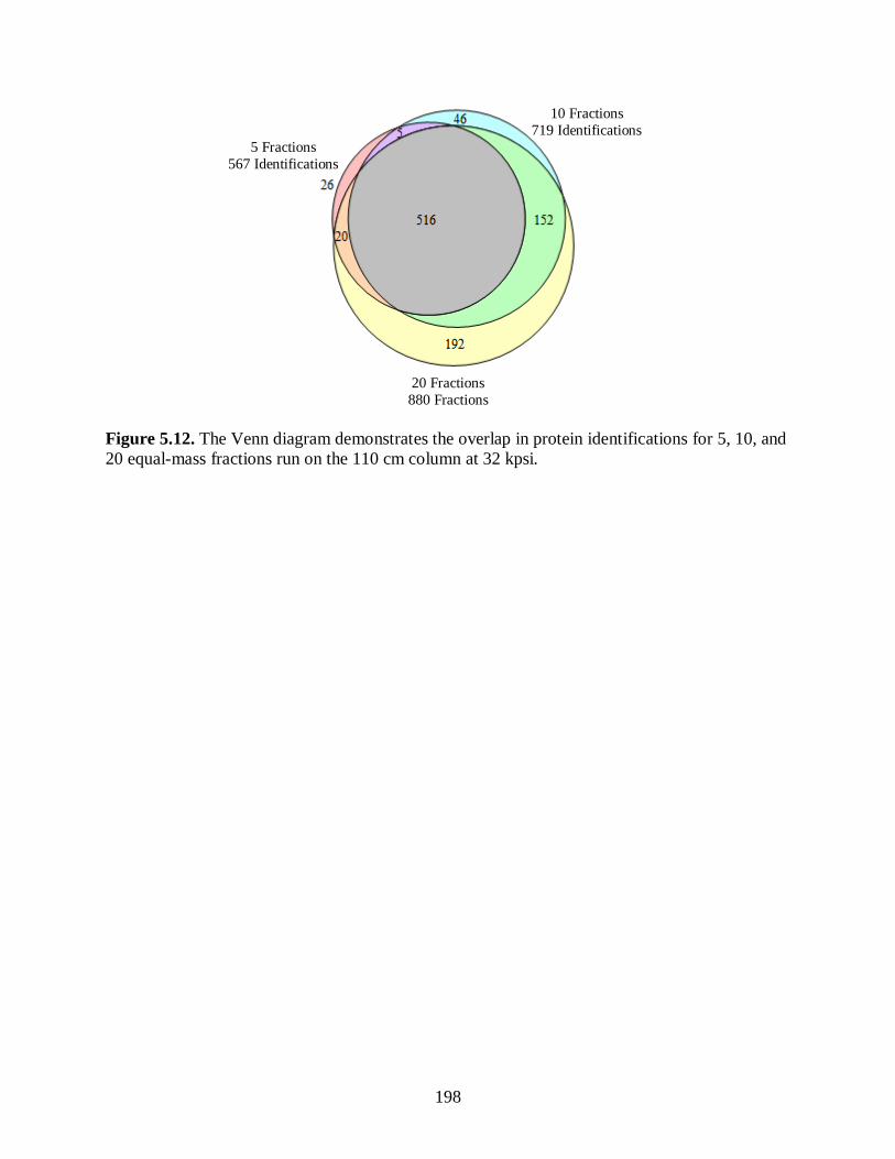
198
10 Fractions
719 Identifications
5 Fractions
567 Identifications
20 Fractions
880 Fractions
Figure 5.12. The Venn diagram demonstrates the overlap in protein identifications for 5, 10, and
20 equal-mass fractions run on the 110 cm column at 32 kpsi.

199
a) Modified UHPLC b) Standard UPLC
Figure 5.13. Fractions per protein describe the percentage of proteins that were identified in one,
two or more (3+) fractions run on the 110 cm column at 32 kpsi (a) and the standard UPLC (b).
As prefractionation frequency increased, more proteins were identified in multiple fractions. A
larger percentage of the proteins were identified in multiple fractions with the modified system.
The increased identification of proteins across multiple fractions was mostly likely related to the
increased peak intensities in the second dimension separation.

200
Figure 5.14. To compare the 5 fractions run on the modified system to the 5 fractions run on the
standard UPLC, the NDPC is plotted with proteins with higher coverage on the left, and proteins
with lower coverage on the right. If a protein was identified with higher sequence coverage when
analyzed on the modified UHPLC, its NDPC value is positive (blue bars). The red bars signify
higher coverage in the analysis on the standard UPLC. Differences in coverage were minimal for
highly covered proteins. As protein coverage decreased, more proteins were identified with
higher coverage from the analysis on the modified UHPLC. The dashed lines indicate a level of
two-fold greater protein coverage. (This was a large graph and split into multiple parts.)

201
Figure 5.14. (continued)

202
Figure 5.14. (continued)

203
Figure 5.14. (continued)

204
Figure 5.14. (continued)

205
a)
b)
c)
Figure 5.15. The NDPC plotted here compare proteins identified with the modified and standard
UHPLCs for 5 (a), 10 (b), and 20 (c) first dimension fractions. If a protein was identified with
higher sequence coverage with the modified UHPLC, the NDPC value is positive (blue lines).
The red lines signify higher coverage with the standard UPLC. Proteins with higher coverage are
plotted on the left, and proteins with lower coverage are on the right. More proteins were
identified with higher coverage by with the modified UHPLC.

206
5.7 REFERENCES
1. Kenyon, G. L.; DeMarini, D. M.; Fuchs, E.; Galas, D. J.; Kirsch, J. F.; Leyh, T. S.; Moos,
W. H.; Petsko, G. A.; Ringe, D.; Rubin, G. M.; Sheahan, L. C., Defining the Mandate of
Proteomics in the Post-Genomics Era: Workshop Report: ©2002 National Academy of
Sciences, Washington, D.C., USA. Reprinted with permission from the National
Academies Press for the National Academy of Sciences. Molecular & Cellular
Proteomics 2002, 1 (10), 763-780.
2. Omenn, G. S., The Human Proteome Organization Plasma Proteome Project pilot phase:
reference specimens, technology platform comparisons, and standardized data
submissions and analyses. PROTEOMICS 2004, 4 (5), 1235-1240.
3. Paik, Y.-K.; Jeong, S.-K.; Omenn, G. S.; Uhlen, M.; Hanash, S.; Cho, S. Y.; Lee, H.-J.;
Na, K.; Choi, E.-Y.; Yan, F.; Zhang, F.; Zhang, Y.; Snyder, M.; Cheng, Y.; Chen, R.;
Marko-Varga, G.; Deutsch, E. W.; Kim, H.; Kwon, J.-Y.; Aebersold, R.; Bairoch, A.;
Taylor, A. D.; Kim, K. Y.; Lee, E.-Y.; Hochstrasser, D.; Legrain, P.; Hancock, W. S.,
The Chromosome-Centric Human Proteome Project for cataloging proteins encoded in
the genome. Nat Biotech 2012, 30 (3), 221-223.
4. Pray, L., Eukaryotic genome complexity. Nature Education 2008, 1 (1).
5. Righetti, P. G.; Campostrini, N.; Pascali, J.; Hamdan, M.; Astner, H., Quantitative
proteomics: a review of different methodologies. Eur J Mass Spectrom (Chichester, Eng)
2004, 10 (3), 335-48.
6. Gilar, M.; Olivova, P.; Daly, A. E.; Gebler, J. C., Two-dimensional separation of peptides
using RP-RP-HPLC system with different pH in first and second separation dimensions.
Journal of Separation Science 2005, 28 (14), 1694-1703.
7. Klose, J., Protein mapping by combined isoelectric focusing and electrophoresis of
mouse tissues. Humangenetik 1975, 26 (3), 231-243.
8. O'Farrell, P. H., High resolution two-dimensional electrophoresis of proteins. Journal of
Biological Chemistry 1975, 250 (10), 4007-4021.
9. Giddings, J. C., Unified separation science. Wiley: 1991.
10. Bushey, M. M.; Jorgenson, J. W., Automated instrumentation for comprehensive two-
dimensional high-performance liquid chromatography of proteins. Analytical Chemistry
1990, 62 (2), 161-167.
11. Sandra, K.; Moshir, M.; D’hondt, F.; Tuytten, .; Verleysen, K.; Kas, K.; François, I.;
Sandra, P., Highly efficient peptide separations in proteomics: Part 2: Bi- and
multidimensional liquid-based separation techniques. Journal of Chromatography B
2009, 877 (11–12), 1019-1039.

207
12. Gilar, M.; Daly, A. E.; Kele, M.; Neue, U. D.; Gebler, J. C., Implications of column peak
capacity on the separation of complex peptide mixtures in single- and two-dimensional
high-performance liquid chromatography. Journal of Chromatography A 2004, 1061 (2),
183-192.
13. Schure, M. R., Limit of Detection, Dilution Factors, and Technique Compatibility in
Multidimensional Separations Utilizing Chromatography, Capillary Electrophoresis, and
Field-Flow Fractionation. Analytical Chemistry 1999, 71 (8), 1645-1657.
14. MacNair, J. E.; Patel, K. D.; Jorgenson, J. W., Ultrahigh-Pressure Reversed-Phase
Capillary Liquid Chromatography: Isocratic and radient Elution Using Columns
Packed with 1.0-μm Particles. Analytical Chemistry 1999, 71 (3), 700-708.
15. Shen, Y.; Zhang, R.; Moore, R. J.; Kim, J.; Metz, T. O.; Hixson, K. K.; Zhao, R.;
Livesay, E. A.; Udseth, H. R.; Smith, R. D., Automated 20 kpsi RPLC-MS and MS/MS
with Chromatographic Peak Capacities of 1 −15 and Capabilities in Proteomics and
Metabolomics. Analytical Chemistry 2005, 77 (10), 3090-3100.
16. Zhou, F.; Lu, Y.; Ficarro, S. B.; Webber, J. T.; Marto, J. A., Nanoflow Low Pressure
High Peak Capacity Single Dimension LC-MS/MS Platform for High-Throughput, In-
Depth Analysis of Mammalian Proteomes. Analytical Chemistry 2012, 84 (11), 5133-
5139.
17. Chen, H.; Horváth, C., High-speed high-performance liquid chromatography of peptides
and proteins. Journal of Chromatography A 1995, 705 (1), 3-20.
18. Franklin, E. G. Utilization of Long Columns Packed with Sub-2 mum Particles Operated
at High Pressures and Elevated Temperatures for High-Efficiency One-Dimensional
Liquid Chromatographic Separations. The University of North Carolina at Chapel Hill,
2012.
19. Thompson, J. D.; Carr, P. W., High-Speed Liquid Chromatography by Simultaneous
Optimization of Temperature and Eluent Composition. Analytical Chemistry 2002, 74
(16), 4150-4159.
20. Neue, U. D., HPLC Columns: Theory, Technology, and Practice. Wiley: 1997.
21. Kelleher, N. L.; Lin, H. Y.; Valaskovic, G. A.; Aaserud, D. J.; Fridriksson, E. K.;
McLafferty, F. W., Top Down versus Bottom Up Protein Characterization by Tandem
High-Resolution Mass Spectrometry. Journal of the American Chemical Society 1999,
121 (4), 806-812.
22. Wolters, D. A.; Washburn, M. P.; Yates, J. R., An Automated Multidimensional Protein
Identification Technology for Shotgun Proteomics. Analytical Chemistry 2001, 73 (23),
5683-5690.
23. Steen, H.; Mann, M., The ABC's (and XYZ's) of peptide sequencing. Nature reviews
Molecular cell biology 2004, 5 (9), 699-711.

208
24. Nesvizhskii, A. I.; Aebersold, R., Interpretation of Shotgun Proteomic Data: The Protein
Inference Problem. Molecular & Cellular Proteomics 2005, 4 (10), 1419-1440.
25. Di Palma, S.; Hennrich, M. L.; Heck, A. J. R.; Mohammed, S., Recent advances in
peptide separation by multidimensional liquid chromatography for proteome analysis.
Journal of Proteomics 2012, 75 (13), 3791-3813.
26. Martosella, J.; Zolotarjova, N.; Liu, H.; Nicol, G.; Boyes, B. E., Reversed-Phase High-
Performance Liquid Chromatographic Prefractionation of Immunodepleted Human
Serum Proteins to Enhance Mass Spectrometry Identification of Lower-Abundant
Proteins. Journal of Proteome Research 2005, 4 (5), 1522-1537.
27. Dowell, J. A.; Frost, D. C.; Zhang, J.; Li, L., Comparison of Two-Dimensional
Fractionation Techniques for Shotgun Proteomics. Analytical Chemistry 2008, 80 (17),
6715-6723.
28. Stobaugh, J. T.; Fague, K. M.; Jorgenson, J. W., Prefractionation of Intact Proteins by
Reversed-Phase and Anion-Exchange Chromatography for the Differential Proteomic
Analysis of Saccharomyces cerevisiae. Journal of Proteome Research 2012, 12 (2), 626-
636.
29. Issaq, H. J.; Chan, K. C.; Janini, G. M.; Conrads, T. P.; Veenstra, T. D.,
Multidimensional separation of peptides for effective proteomic analysis. Journal of
Chromatography B 2005, 817 (1), 35-47.
30. Vestling, M. M.; Murphy, C. M.; Fenselau, C., Recognition of trypsin autolysis products
by high-performance liquid chromatography and mass spectrometry. Analytical
Chemistry 1990, 62 (21), 2391-2394.
31. Fersht, A., Structure and Mechanism in Protein Science: A Guide to Enzyme Catalysis
and Protein Folding. W. H. Freeman: 1999.
32. Aguilar, M. I., HPLC of Peptides and Proteins: Methods and Protocols. Humana Press:
2004.
33. Searle, B. C., Scaffold: A bioinformatic tool for validating MS/MS-based proteomic
studies. PROTEOMICS 2010, 10 (6), 1265-1269.
34. Eng, J. K.; Searle, B. C.; Clauser, K. R.; Tabb, D. L., A Face in the Crowd: Recognizing
Peptides Through Database Search. Molecular & Cellular Proteomics 2011, 10 (11).
35. Wagner, A., Energy Constraints on the Evolution of Gene Expression. Molecular Biology
and Evolution 2005, 22 (6), 1365-1374.
209
CHAPTER 6. Multidimensional Separations at 32 kpsi using Long Microcapillary
Columns for the Differential Proteomics Analysis of Saccharomyces cerevisiae
6.1 Introduction
The study of protein expression has been important in understanding biological pathways.
Studying the differential protein expression of an organism with two different phenotypes has
brought light to the role proteins play in these pathways.1,2
Saccharomyces cerevisiae, commonly
known as baker’s yeast, is a model organism for testing new analysis methods because its
proteome is relatively well understood.3 The validity of several common proteomics methods
was first demonstrated by analyzing baker’s yeast.4,5
Since the yeast proteome is a complex
biological mixture, many of these methods begin with a separation by liquid chromatography
(LC) before analysis by mass spectrometry (MS).6
Though great improvements have been made in the field of liquid chromatography,7,8
no
single separation exists with the peak capacity necessary to effectively separate an entire
proteome.9 Multidimensional separations were developed as a means to improve peak capacity.
10
Early multidimensional separations coupled a long size exclusion or cation-exchange column to
a reversed phase column.11,12,13
Other scientists packed biphasic columns with reversed phase
sorbent at the outlet and strong cation-exchange sorbent at the inlet to separate proteome
digests.14,15
More recent work focused on the separation of intact proteins by three modes before
analysis by ESI-FTICR-MS. The three separation modes included two electrophoretic
separations by isoelectric focusing and size followed by reversed-phase LC.16,17

210
To aid in sample solubility, proteomics experiments commonly start with digestion prior to
separation. This shotgun approach increases the complexity of the biological mixture prior to
analysis.18
More recently, a prefractionation approach has been implemented in which the intact
proteins are fractionated by the first dimension separation, and fractions are enzymatically
digested prior to analysis by LC-MS.19,20
Experimentally, prefractionation methods are more
orthogonal than other multidimensional separations because the sample is completely changed
via digestion between separations.21
Digestion between the separations enables the use of
reversed phase columns in both dimensions which tend to have higher peak capacity than other
LC separation modes such as ion exchange and size exclusion chromatography.22
The number of
fractions collected will determine the peak capacity of the first dimension separation. However,
high prefractionation frequencies will increase analysis time and increase the probability of
splitting a protein between two fractions, and thus dilute the analyte. A study of prefractionation
frequency was completed in Chapter 5. The results indicated that five fractions yielded adequate
information about the yeast proteome if a long microcapillary column is used in the second
dimension.
In concert with improvements to separation techniques, scientists have improved mass
spectrometric detection of large biomolecules. The development of ion mobility added a post
ionization separation.23
High resolution mass spectrometers such as FTICR and especially
orbitraps have become more common laboratory instruments.24
Time-of-flight (TOF)
instruments are also widely used for proteomics experiments.25
However, ionization suppression
and matrix effects still plague mass spectrometric techniques, necessitating separation prior to
analysis.26,27
211
To help with the quantitative analysis of mass spectral data, many sample labeling
techniques such as iTRAQ and SILAC have been developed. However, the label-free technique
remains popular for relative quantification.28
The major advantage to label-free relative
quantification is that no further manipulation of the sample is required. Also, the spectra are not
busy with isobaric and isotopic data. The validity of quantification based on spectral counts with
the label-free method has been demonstrated in the literature.14,15,24
The differential study in this manuscript investigated yeast grown on dextrose and
glycerol. Dextrose is the preferred growth medium. Growth on an alternative carbon source
yields protein expressions characteristic of an environmental stress response.29
A previous study
of this differential expression from the Jorgenson Lab separated the soluble portion of the yeast
proteome by RPLC into 20 equal-time fractions. The fractions were digested before analysis by a
standard UPLC-qTOF-MS.21
Herein, a method is described which samples the first dimension by
equal-mass prefractionation into just five fractions. A UHPLC capable of separations above 30
kpsi increased the peak capacity of the second dimension separation. This prefractionation
experiment reduced the previously reported separation time by four fold. With the improved
separation, 527 proteins were identified in the dextrose sample and 539 in the glycerol sample
which is more than the previously reported analysis.
6.2 Materials and method
6.2.1 Materials
Water, acetonitrile, isopropyl alcohol and ammonium hydroxide were purchased from
Fisher Scientific (Fair Lawn, NJ). Ammonium acetate, ammonium bicarbonate, formic acid,
trifluoroacetic acid and iodoacetamide were purchased from Sigma-Aldrich Co. (St. Louis, MO).
RapigestTM
SF acid-labile surfactant and bovine serum album digest standard (BSA) were

212
obtained from Waters Corporation (Milford, MA). Dithiothreitol was purchased from Research
Products International (Mt. Prospect, IL), and TPCK-modified trypsin was purchased from
Pierce (Rockford, IL). Water and acetonitrile were Optima LC-MS grade, and all other chemicals
were ACS reagent grade or higher. Growth, harvesting, and lysis of S. cerevisiae from glycerol
and dextrose media were previously described.21
6.2.2 Intact protein prefractionation
The prefractionation of intact proteins, outlined in Figure 6.1., was performed on a 4.6 x
250 mm PLRP-S column with 5 µm particles (Agilent, Santa Clara, CA) heated to 80 °C. Four
milligrams of total protein were injected onto the column. The gradient profile is shown in Table
6.1. The separation was followed by UV spectrophotometry to give a qualitative chromatogram
of the separation. The wavelength was set to 214 nm, which is the lambda max of the peptide
bond. One-minute wide fractions, containing 1 mL of effluent each, were collected in
microcentrifuge tubes. To concentrate the fractions, they were lyophilized and then reconstituted
in 25 µL of 5 mM ammonium bicarbonate. Three microliters of 6.6 % (w/v) api est™ SF in
buffer were added. Solutions were vortexed, sonicated for 15 minutes, and incubated at 80 ºC for
15 minutes to denature the proteins..
6.2.3 Equal-mass prefractionation
To determine fractionation by equal-mass, each absorbance value for the UV
chromatogram was summed with all previous absorbance values from 10 to 48 minutes which
corresponded to the time after the injection plug until just before the wash. Summed absorbance
was calculated as follows
Summed Absorbance (ΣA) ∑ At
td tg
td (6-1)

213
where A = absorbance, t = time, td = dead time, and tg = gradient time. The Σ absorbance
was normalized and plotted versus first dimension separation time in Figure 6.2. The
Σ absorbance was divided into increments of 0.05 which split the axis into 20 even parts. The
times associated with the 20 Σ absorbance values were rounded to the nearest minute. These
times were used to redistribute the 38 one-minute-wide fractions into 20 equal-mass fractions.
Each of the 20 fractions has an equal-mass of total protein but a varying amount of solvent.
6.2.4 Protein digestion
The digestion is more efficient when carried out in a minimal amount of solvent.
Therefore, the 20 equal-mass fractions were also lyophilized and reconstituted in 25 µL of 50
mM ammonium bicarbonate. Three microliters of 6.6 % (w/v) api est™ SF in buffer were
added. Solutions were vortexed, sonicated for 15 minutes, and incubated at 80 ºC for 15 minutes
to denature the proteins. The proteins were reduced by adding 1 µL of 100 mM dithiothreitol,
vortexed, sonicated for 5 minutes, and incubated for 30 min at 60ºC. Proteins were then alkylated
with 1 µL of 200 mM iodoacetamide, vortexed, sonicated for 5 minutes, and stored protected
from light for 30 min at room temperature. The proteins were then digested by adding 10 µL of
667 ng/µL TPCK-modified trypsin in 50 mM ammonium bicarbonate, pH 8 (overnight, 37ºC).
The trypsin amount was approximated to be a 50:1 (w/w) protein to enzyme ratio if the initial
protein amount was equally distributed across the 20 fractions. The digestion was quenched, and
the api est™ SF was degraded using 44 µL 8:1:1 (v:v:v) water:acetonitrile:trifluoroacetic
acid (45 min, 37ºC). The fractions were centrifuged for 10 minutes at 14,000 Xg to pellet the
hydrolyzed surfactant, after which they were ready for analysis. The samples were transferred to
LC vials and spiked with 1.3 µL of a 1 pmol/L internal standard BSA digest (Waters).

214
To form the sets of 5 fractions, 20 µL of every four consecutive fractions from the set of
20 were combined, lyophilized, and reconstituted with 10 µL 50 mM ammonium bicarbonate
and 10 µL 98:1:1 (v:v:v) water:acetonitrile:trifluoroacetic acid. The fractionation schemes are
outlined in Table 6.2.
6.2.5 Peptide analysis by UHPLC-MSE
Each fraction was analyzed in triplicate by capillary RPLC-MS using the UHPLC system
described in Chapter 3 coupled to a QTOF Premier MS. Mobile phase A was Optima Grade
water with 0.1% formic acid (Fisher), and mobile phase B was Optima-grade acetonitrile with
0.1% formic acid (Fisher). The samples were pre-concentrated on a 110 cm x 75 µm ID, 1.9 µm
BEH C18 column with 0.5% mobile phase B, and then separated with a 25 µL gradient from 4-
40%B followed by a wash at 85% and equilibration at initial conditions. The gradient program is
listed in Table 6.3. The column was run at 32 kpsi at 65°C to produce a 300 nL/min flow rate.
The outlet of the RPLC column was connected via a 30 cm x 20 µm ID piece of silica capillary
to an uncoated fused silica nanospray emitter with a 20 µm ID and pulled to a 10 µm tip (New
Objective, Woburn, MA) operated at 2.6 kV. Data-independent acquisition (MSE) was performed
with the instrument set to acquire parent ion scans from m/z 50-1990 over 0.6 sec at 5.0 V. The
collision energy was then ramped from 15-40 V over 0.6 sec with 0.1 sec interscan delay.
6.2.6 Peptide data processing
The peptide LC-MS/MS data were processed using ProteinLynx Global Server 2.5
(Waters). The MSE spectra were searched against a database of known yeast proteins from the
Uni-Prot protein knowledgebase ( www.uniprot.org) with a reversed sequence appended to the
end. The false discovery rate was set to 100% to yield data compatible for further processing.

215
After the database search was complete, the results were imported into Scaffold 4.2.0
(Proteome Software, Portland, OR). The minimum protein probability and peptide probability
filters were set to a 5% false discovery rate, and a minimum of three peptides were required to
identify a protein. Peptides matching multiple proteins were exclusively assigned to the protein
with the most evidence. The proteins were quantified by the normalized total precursor intensity.
The precursor intensities assigned to a protein were totaled to give the quantitative value of that
protein. The values were normalized by subtracting each sample’s median log intensity then
adding back the median log intensity for all samples.30,31,32,33
A student’s 2-sided t-test was
performed on the triplicate samples. Proteins with a p-value less than 0.050 between the two
yeast samples and a fold change greater than 2.0 were considered to be differentially expressed
with 95% confidence or greater.
6.3 Discussion
Reversed-phase prefractionation of the lysate from yeast grown on dextrose and glycerol
produced 38 one-minute-wide fractions. Measures were taken during method development to
evenly distribute the proteins across the first dimension separation. However, most observed
peaks from the first dimension chromatogram occurred in the middle of the retention window.
Analysis of all 38 fractions would be unproductive as many proteins were undoubtedly split
between multiple fractions diluting the analyte. Fractions with less intense first dimensional
peaks would yield little information in the second dimension analysis. The offline nature of this
multidimensional separation gave us flexibility to further process the fractions before second
dimension analysis. For these reasons, the fractions were recombined into equal-mass fractions
before digestion, as outlined in Table 6.2.

216
According to the prefractionation frequency study in Chapter 5, it was determined that 5
fractions were adequate to yield sufficient information from the yeast proteome when fractions
were run on a long, 110 cm microcapillary column at 32 kpsi. The multidimensional
chromatograms are shown in Figure 6.3. From these plots, it is observed that the separation space
was well utilized, peaks fill most of the 2D space, and the peaks are orthogonal.
6.3.1 Protein prefractionation
To more deeply analyze the first dimension separation, the resulting chromatograms are
overlaid onto bar graphs in Figure 6.4. The number of proteins identified in each fraction is
displayed for yeast grown on dextrose (a) and glycerol (b). Between 96 and 176 total proteins
were identified per fraction as drawn with light gray bars. Unique identifications are drawn with
dark gray bars. The total protein count was defined as any protein found within a given fraction;
thus, if a protein were to be found in multiple fractions it would be counted in each fraction. The
unique protein values count each protein entry only once. A protein identified in multiple
fractions is assigned to the fraction in which it had the highest quantitative value. Between 55
and 122 unique proteins were identified per fraction. The area under the first dimension
chromatogram should be equal for each fraction. There were few peaks towards the end of the
chromatogram so a large portion of the first dimension separation was pooled into one fraction.
A large number of proteins were identified from peptide analysis of the last fraction. By pooling
this area into one fraction, information can be gained about the yeast proteome without a large
commitment of analysis time.
The crowded and over lapping peaks in the first dimension separation prohibited the
measurement of peak widths. As an alternative, the number of fractions per protein, as shown in
Figure 6.5., was used to describe in how many first dimension fractions a protein was identified.

217
Most proteins were identified in only one fraction. For yeast on dextrose, 68% of the proteins
were identified in only one fraction, 16% were identified in two fractions, and the remaining
16% were identified in three or more fractions. Similarly for yeast grown on glycerol, 66% of the
proteins were identified in one fraction, 19% were identified in two fractions, and 14% were
identified in three or more fractions. This was a slight improvement over our lab’s previous
results in which 60% of the proteins were identified in one fraction, 20% were identified in two
fractions, and 20% were identified in three or more fractions.21
Our previous method had twenty
first dimension fractions which increased the odds of splitting first dimension protein peaks
between multiple fractions. The improvement was only slight because the intensities of the
second dimension peptide peaks were much greater for the experiment described in this
manuscript. With a longer column run at higher pressure, peaks were narrower and more intense
increasing the likelihood of identifying proteins with lower abundance in multiple factions (See
Chapter 5).
6.3.2 Benefits of increasing second dimension peak capacity
The total number of proteins identified in the dextrose and glycerol sample was 527 and
539, respectively, with 350 or 65% of the proteins being identified in both samples as portrayed
by the Venn diagram in Figure 6.6. These results were similar to our previously reported
differential proteomics study using the prefractionation method.21
However, the peak capacity of
the second dimension separation described in this chapter was approximately 450, about
2.5 times the peak capacity of our earlier work, even though second dimension separation times
were similar. The gain in second dimension peak capacity took burden off the prefractionation
step. Therefore, more information could be elucidated out of only five fractions as opposed to the
20 fractions described previously.

218
The theoretical two-dimensional peak capacity was 2,250 with this experiment and 4,000
for our earlier experiment.21
The experiment described here better distributed the sample
throughout the multidimensional separation space which would increase fractional coverage.
Stoll and coworkers suggested multiplying the theoretical peak capacity by the fractional
coverage factor to give a better estimate of the practical peak capacity for 2D separations.34
The
results from Chapter 2 suggested that improving peak capacity in the first dimension alone had a
limit as to how many proteins may be identified. Proteomics experiments involve many steps and
techniques. Improvements to not one but all techniques will be necessary to more deeply mine
information from the proteome. Ultrahigh pressure separation on long, microcapillary columns
increased to the number of proteins identified and decreased total separation time.
6.3.3 Increasing protein coverage
The improvements to the multidimensional separation did not only improve the number
of protein identifications but also the protein coverage. The coverage and number of peptides
identified for several proteins involved in yeast metabolism are listed in Table 6.4. Chapter 2
proposed the Normalized Difference Protein Coverage (NDPC) to compare protein coverage
between multiple methods. The same metric was used to compare the difference in coverage for
proteins identified in this chapter and our earlier work21
normalized by the total coverage
between both experiments. The Grand NDPC combines the NDPC for all proteins into a single
value by calculating the difference between the grand total protein coverage normalized by the
grand sum of protein coverage in both methods as follows:
rand NDPC (∑CoverageChapter 6)-(∑CoverageLiterature)
∑CoverageChapter 6 ∑CoverageLiterature (6-2)

219
The Grand NDPC can be related to a Fold-Change in Coverage as follows:
Fold-Change in Coverage ∑Coverage
method 1
∑Coveragemethod 2
1 rand NDPC
1- rand NDPC (6-3)
If the fold-change is less than one, the negative reciprocal of the value is used as is
conventional with fold-change calculations. The Grand NDPC and Fold-Change in Coverage are
listed in Table 6.5. The positive values represent higher coverage with the 5 equal-mass fractions
run on the 110 cm long column at 32 kpsi as described in this chapter. A negative value would
have indicated higher coverage by our previous results from the 20 equal-time fraction run on the
25 cm commercial column at 8 kpsi on the standard UPLC.21
The improvement is small but
impressive when one considers that separation time was reduced four fold.
6.3.4 Differential proteins
The differential proteins were qualified with a fold change of greater than two and a p-
value of less than 0.05 which corresponds to a negative log10 p-value of 1.3 and 95% confidence.
The volcano plot in Figure 6.7.a. graphs the negative log10 p-value versus log2 fold change. A
negative or positive fold change is a convention for up-regulation of the protein in yeast grown
on dextrose or glycerol, respectively. The points in the upper left and right of the plot represent
proteins with the largest difference in abundance between the two samples and with the most
confidence. Protein quantity is not captured in the volcano plot so the log quantitative values of
all significantly different proteins are plotted in Figure 6.7.b. Proteins up-regulated in the
dextrose or glycerol sample are closer to the y-axis or x-axis, respectively. Points falling along
the axes were only identified in the sample corresponding to that axis. There were 274 proteins
that were determined to be significantly different. The most interesting of these proteins would
have a large abundance in only one sample and are represented by points in the top-left and
bottom-right of Figure 6.7.b.

220
Of the significantly different proteins, several were identified to be part of the metabolic
pathways of yeast which, according to the literature, would have differences in expression when
exposed to different carbon sources.35
Proteins involved in the metabolic pathways of interest are
listed in Table 6.6. with their associated p-value, intensity, and fold change. Several metabolic
pathways of S. cervisiae including glycerol catabolism/glycerolneogenesis, glycolysis/
gluconeogenesis, fermentation, the TCA cycle, and the glyoxylate cycle are depicted in Figure
6.8. Proteins identified in blue or red represent up-regulation of the protein in yeast which was
grown on the dextrose or glycerol media, respectively. The differential protein fold-changes
measured by the methods described here follow the trends in protein expression predicted by the
literature for growth in dextrose deficient media which will invoke an environmental stress
response.35
Glycolysis is the digestion of glucose to pyruvate, which can then be converted into
energy through the TCA cycle, glyoxylate cycle, or fermentation. The first step in glycolysis is to
phosphorylate glucose with the hexokinase family of enzymes (HXKA, HXKB). Glucokinase
(HXKG) has a slightly different role because it acts as a regulator for glucose consumption.
Previous studies reported increased transcription of glucokinase when yeast was grown on
glycerol36,37
which was confirmed in the results from this study.
In the pathway from glucose to pyruvate are the transketolase (TKT1, TKT2) and
transaldolase (TAL1, TAL2) protein families. These proteins are also involved in metabolizing
carbon energy sources through the pentose phosphate pathway (PPP). In normal cell function,
TKT1 and TAL1 are the predominant proteins involved in the conversion of fructose-6-P to
glyceraldehyde-3-P.38,39
TKT1 and TAL1 were identified by this method but not differentially. In
the absence of glucose, it has been previously concluded that TKT2 will dominate the conversion

221
of fructose-6-P to glyceraldehyde-3-P. The literature is inconclusive on the role of TAL2.40
The
results from this manuscript found both TKT2 and TAL2 proteins to be up-regulated in yeast
grown on glycerol.
Through the pentose phosphate pathway (PPP), glucose is transformed into ribulose-5-
phosphate which is a step in the formation of ribonucleic acids and ribosomal proteins. Cells
grown under stress conditions, such as a dextrose deficient environment, will exhibit a lack of
ribosomal protein.29
Therefore, an abundance of ribosomal proteins should exist in the yeast
grown on dextrose. A total of 67 ribosomal proteins were identified with 19 up-regulated and
only one down-regulated in the dextrose sample.
Analogous to glycolysis is glycerol metabolism, which converts glycerol into pyruvate.
For the yeast grown on glycerol, it is predicted that the proteins used in glycerol catabolism such
as GLPK and GPD1 would be up-regulated41,42
while the proteins used in glycerolneogenesis,
such as GPP1 and GPP2, would be down-regulated.43
This phenomenon was observed for
GLPK, GPD1 and GPP1. No significant difference was observed for GPP2 and GPD2
expression.
After its biogenesis, pyruvate is fermented into ethanol if there is an excess amount of
glucose present. A protein complex is formed by PDC1, PDC5 and PDC6. This complex is
involved in the conversion of pyruvate to acetaldehyde during fermentation.44
These three
subunits were identified with PDC5 and PDC6 being up-regulated in the dextrose sample.
Acetaldehyde is then converted into ethanol. The alcohol dehydrogenases (ADH1, ADH3,
ADH6) involved in the conversion were all identified with ADH6 being more abundant in yeast
grown on dextrose.

222
In the absence of dextrose, pyruvate enters the TCA and glyoxylate cycles45
which can
occur directly by conversion to oxaloacetate with pyruvate carboxylases (PYC1, PYC2) or
through the acetyl-CoA bypass mechanism involving pyruvate dehydrogenase (ODPB) and
dihydrolipoyl dehydrogenase (DLDH). Additionally, any ethanol that may be present is
metabolized by alcohol dehydrogenase (ADH2), aldehyde dehydrogenases (ALDH2, ALDH4)
and acetyl-coenzyme A synthetase (ACS1) for entrance into the TCA or glyoxylate
cycle.42,46,47,48,49
Of the 24 proteins involved in processing pyruvate through the TCA and
glyosylate cycles, 18 were significantly more abundant in the yeast grown on glycerol. The other
six proteins showed no significant fold change in abundance between the two samples.
The roles of ALDH5 and ACS2 are not completely defined in the literature but some
studies indicate that their function differs from that of other aldehyde dehydrogenases and acetyl-
coenzyme A synthetases.50
One theory is that ALDH5 and ACS2 regulate ethanol to keep it
below toxicity levels, maintaining a healthy environment for the biosynthesis other metabolites
important to cell growth.51,52
In this experiment, ALDH5 and ACS2 were found to be up-
regulated in dextrose.
A final difference between yeast grown on alternative carbon sources is the location of
metabolism in the cell. Fermentation with dextrose occurs in the cytoplasm, while the TCA and
glyoxylate cycles, metabolizing glycerol, occur in the mitochondria.53
To support increased
activity in the mitochondria, more mitochondrial proteins would have to be transcribed. The
results from this study identified 65 mitochondrial proteins with 26 up-regulated and only one
down-regulated in the yeast sample grown on glycerol.
223
6.4 Conclusions
The multidimensional UHPLC-MS analysis identified 527 proteins in yeast grown on
dextrose and 539 proteins in yeast grown on glycerol. The differential abundances were
determined for many proteins involved in yeast metabolism of the two different carbon sources.
By utilizing the first dimension chromatographic intensity to prefractionate the sample by equal-
mass, the digestion was improved by better estimating the protein to enzyme ratio. This
prefractionation technique better estimated column loading for the second dimension and
improved the practical peak capacity of the multidimensional separation. Increased peak capacity
of the second dimension separation, with a long microcapillary column run at elevated pressure,
reduced the need for a high prefractionation frequency without reducing the number of protein
identifications. With fewer first dimension fractions, analysis time was decreased by 75% as
compared to a previously reported study by the Jorgenson Lab.21
Proteomic experiments involve
many steps and techniques. Improvements to not one but all techniques will be necessary to more
deeply mine information from the proteome. Ultrahigh pressure separations on long,
microcapillary columns provided improvement to the number and coverage of proteins
identifications in a differential proteomics analysis of S. cerevisiae.
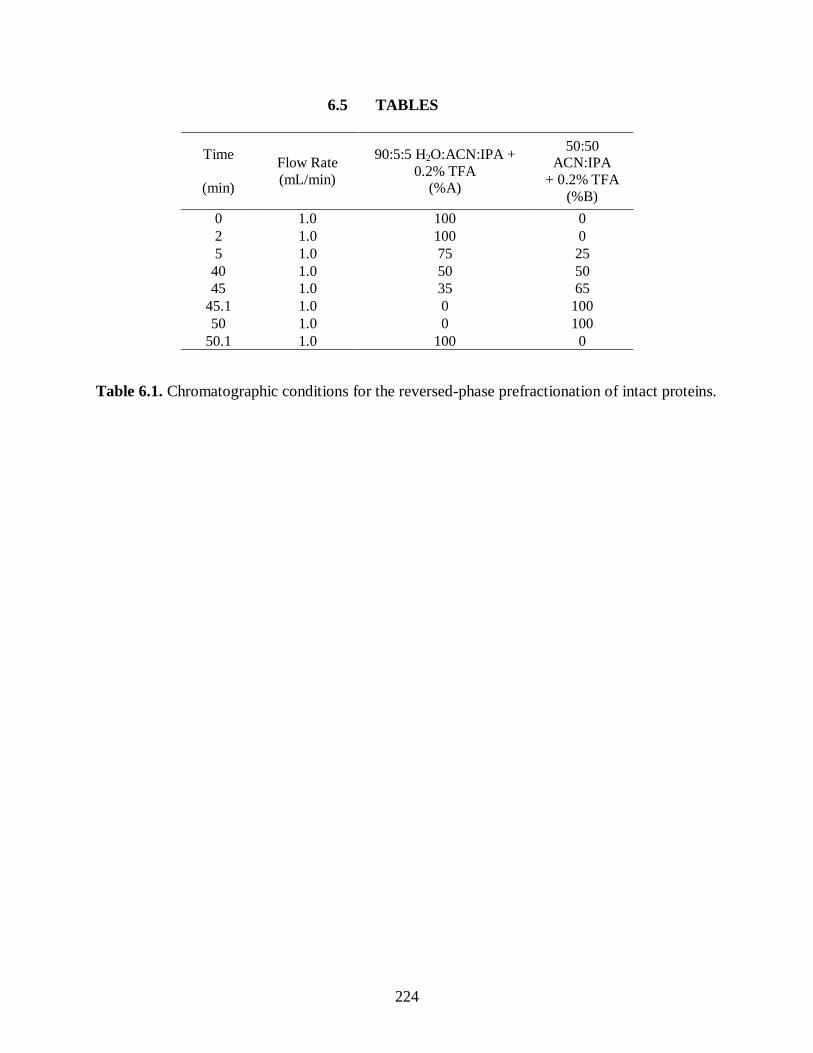
224
6.5 TABLES
Time
(min)
Flow Rate
(mL/min)
90:5:5 H2O:ACN:IPA +
0.2% TFA (%A)
50:50 ACN:IPA
+ 0.2% TFA
(%B)
0 1.0 100 0
2 1.0 100 0
5 1.0 75 25
40 1.0 50 50
45 1.0 35 65
45.1 1.0 0 100
50 1.0 0 100
50.1 1.0 100 0
Table 6.1. Chromatographic conditions for the reversed-phase prefractionation of intact proteins.
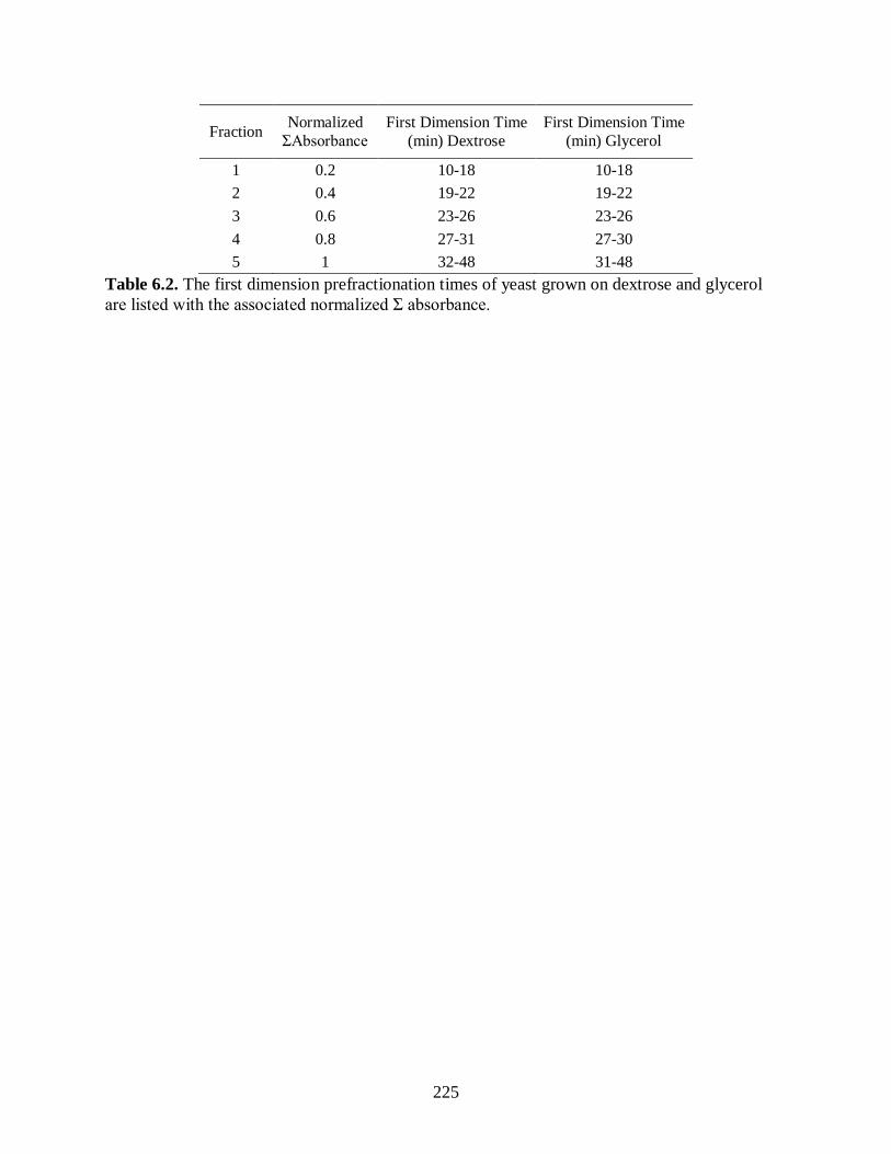
225
Fraction Normalized
ΣAbsorbance
First Dimension Time
(min) Dextrose
First Dimension Time
(min) Glycerol
1 0.2 10-18 10-18
2 0.4 19-22 19-22
3 0.6 23-26 23-26
4 0.8 27-31 27-30
5 1 32-48 31-48
Table 6.2. The first dimension prefractionation times of yeast grown on dextrose and glycerol
are listed with the associated normalized Σ absorbance.

226
Time
(min)
Flow
Rate
(µL/min)
% Mobile
Phase A
% Mobile
Phase A Curve
NanoAcquity
Vent Valve
High Pressure Isolation Valve
Freeze/Thaw Valve
&Vent Valve
Pneumatic Amplier
Pump Initiation
Gradient Loading Method
Initial 5 96.0 4.0 - Off On Off
1.0 5 15.0 85 11 Off On Off 1.8 5 60.0 40 11 Off On Off 6.8 5 96.0 4 6 Off On Off 7.4 5 99.5 0.5 11 Off On Off 8.0 4 99.5 0.5 11 Off On Off 8.1 3 99.5 0.5 11 Off On Off 8.2 2 99.5 0.5 11 Off On Off 8.3 1 99.5 0.5 11 Off On Off 8.4 0.01 99.5 0.5 11 Off On Off 9.0 (end) 0.01 99.5 0.5 11 Off On Off Sample Loading Method
Initial 0.01 99.5 0.5 - Off On Off
0.1 1 99.5 0.5 11 Off On Off 0.2 2 99.5 0.5 11 Off On Off 0.3 3 99.5 0.5 11 Off On Off 0.4 4 99.5 0.5 11 Off On Off 0.5 5 99.5 0.5 11 Off On Off 2.0 5 99.5 0.5 11 Off On Off 2.5 0.01 50 50 11 On Off Off 5.0 0.01 50 50 11 On Off On
35.0 (end) 0.01 50 50 11 On Off On
Ultra High Pressure Separation Method
Initial 0.01 50 50 11 On Off On 150.0 0.01 96 4 11 On On Off
155.0 (end) 0.01 96 4 11 On On Off
Table 6.3. The method for the second dimension separation at ultrahigh pressure, as programmed into MassLynx, is listed along with
the valve timings.

227
Coverage (%)
Assigned Peptides
Name Accession
Dextrose Glycerol
Dextrose Glycerol
Isocitrate lyase ACEA
- 32
- 15
Aconitate hydratase ACON
35 58
23 48 Acetyl-coenzyme A synthetase 1 ACS1
- 57
- 51
Acetyl-coenzyme A synthetase 2 ACS2
28 6
10 1 Alcohol dehydrogenase 1 ADH1
71 73
24 23
Alcohol dehydrogenase 2 ADH2
55 75
27 41 Alcohol dehydrogenase 3 ADH3
28 29
5 9
Alcohol dehydrogenase 6 ADH6
20 -
4 - Aldehyde dehydrogenase 2 ALDH2
5 24
1 10
K-activated aldehyde dehydrogenase ALDH4
38 87
21 53 Aldehyde dehydrogenase 5 ALDH5 21 - 8 - Fructose-bisphosphate aldolase ALF
81 69
30 28
Citrate synthase CISY1
18 61
7 34 Succinate dehydrogenase DHSA
- 20
- 8
Dihydrolipoyl dehydrogenase DLDH
- 63
- 31 Enolase 1 ENO1
84 85
18 22
Enolase 2 ENO2
92 87
54 47 Fumarate reductase FRDS
44 45
15 17
Fumarate hydratase FUMH
6 50
2 22 Glyceraldehyde-3-P dehydrogenase 1 G3P1
66 92
33 45
Glyceraldehyde-3-P dehydrogenase 2 G3P2
91 88
11 9 Glyceraldehyde-3-P dehydrogenase 3 G3P3
94 92
27 25
Glucose-6-phosphate isomerase G6PI
70 56
45 32 Glycerol-3-phosphate dehydrogenase GPD1
8 60
2 23
Glycerol-3-phosphate dehydrogenase GPD2
- 7
- 1 Glycerol-3-phosphatase 1 GPP1
86 -
22 -
Glycerol-3-phosphatase 2 GPP2
15 -
2 - Hexokinase-1 HXKA
34 65
12 24
Hexokinase-2 HXKB
66 70
30 31 Glucokinase-1 HXKG
12 72
3 39
Isocitrate dehydrogenase 1 IDH1
45 60
15 23 Isocitrate dehydrogenase 2 IDH2
6 71
1 17
6-phosphofructokinase subunit α K6PF1
60 52
61 54 Pyruvate kinase 1 KPYK1
86 85
58 53
Malate synthase 1 MASY
- 42
- 22 NAD-dependent malic enzyme MAOM
8 -
4 -
Malate dehydrogenase, cyto MDHC
- 45
- 13 Malate dehydrogenase, mito MDHM
56 75
14 22
2-oxoglutarate dehydrogenase E1 ODO1
- 31
- 25 γ-glutamyl phosphate reductase ODO2
- 40
- 12
Pyruvate dehydrogenase E1 comp β ODPB
48 43
13 10 Phosphoenolpyruvate carboxykinase PCKA
2 74
1 47
Pyruvate decarboxylase isozyme 1 PDC1
75 66
46 39 Pyruvate decarboxylase isozyme 5 PDC5
36 -
12 -
Pyruvate decarboxylase isozyme 6 PDC6
43 23
13 6 Phosphoglycerate kinase PGK
92 89
58 54
Phosphoglycerate mutase 1 PMG1
84 82
29 26 Pyruvate carboxylase 1 PYC1
9 32
8 31
Pyruvate carboxylase 2 PYC2
11 21
3 4 Succinyl-CoA ligase subunit α SUCA
40 71
10 20
Succinyl-CoA ligase subunit β SUCB
- 38
- 25
Transaldolase 1 TAL1
68 66
28 20 Transaldolase 2 TAL2
- 59
- 16
Transketolase 1 TKT1
65 52
36 34 Transketolase 2 TKT2
- 21
- 10
Triosephosphate isomerase TPIS
89 90
28 27
Table 6.4. The protein coverage (%) and number of peptides used to identify each protein are
reported for the some of the proteins involved in S. cerevisiae metabolism.

228
Sample Grand NDPC Fold Change In Coverage
Dextrose 0.074 1.1
Glycerol 0.033 1.1
Table 6.5. The Grand NDPC and Fold-Change in Coverage are listed for each fractionation
frequency. The positive values represent higher coverage with the 5 equal-mass fractions run on
the 110 cm long column at 32 kpsi as described in this chapter. A negative value would have
indicated higher coverage by our previous results from the 20 equal-time fraction run on the 25
cm commercial column at 8 kpsi on the standard UPLC.21
The improvement is small but
impressive when one considers that the total separation time was reduced four fold.

229
Quantitative Value
Name Accession
T-Test P-Value Fold Change
Dextrose Glycerol
Isocitrate lyase ACEA
0% 0.082000 -
n.d. 857
Aconitate hydratase ACON
95% < 0.00010 4.8
2204 10493 Acetyl-coenzyme A synthetase 1 ACS1
95% < 0.00010 G Only
n.d. 20339
Acetyl-coenzyme A synthetase 2 ACS2
95% 0.020000 -9.0
663 73 Alcohol dehydrogenase 1 ADH1
0% 0.530000 -
53597 50028
Alcohol dehydrogenase 2 ADH2
95% 0.000300 4.2
22123 93634 Alcohol dehydrogenase 3 ADH3
0% 0.080000 -
848 1825
Alcohol dehydrogenase 6 ADH6
95% 0.001800 D Only
612 n.d. Aldehyde dehydrogenase 2 ALDH2
95% 0.000150 20.4
32 658
K-activated aldehyde dehydrogenase ALDH4
95% < 0.00010 46.1
2099 96753 Aldehyde dehydrogenase 5 ALDH5 95% 0.0048 D Only 183 n.d. Fructose-bisphosphate aldolase ALF
0% 0.420000 -
34954 30292
Citrate synthase CISY1
95% < 0.00010 41.3
301 12399 Succinate dehydrogenase DHSA
95% 0.005100 G Only
n.d. 419
Dihydrolipoyl dehydrogenase DLDH
95% 0.000130 G Only
n.d. 8330 Enolase 1 ENO1
0% 0.310000 -
54308 65808
Enolase 2 ENO2
0% 0.130000 -
74304 56488 Fumarate reductase FRDS
0% 0.830000 -
908 884
Fumarate hydratase FUMH
95% 0.000540 40.3
117 4725 Glyceraldehyde-3-P dehydrogenase 1 G3P1
0% 0.068000 -
47511 62124
Glyceraldehyde-3-P dehydrogenase 2 G3P2
0% 0.680000 -
61006 57022 Glyceraldehyde-3-P dehydrogenase 3 G3P3
0% 0.081000 -
92025 100055
Glucose-6-phosphate isomerase G6PI
95% 0.009400 -2.8
37367 13228 Glycerol-3-phosphate dehydrogenase GPD1
95% 0.002200 80.0
52 4163
Glycerol-3-phosphate dehydrogenase GPD2
0% 0.370000 -
n.d. 118 Glycerol-3-phosphatase 1 GPP1
95% < 0.00010 D Only
6633 n.d.
Glycerol-3-phosphatase 2 GPP2
0% 0.370000 -
778 n.d. Hexokinase-1 HXKA
0% 0.095000 -
2652 14030
Hexokinase-2 HXKB
0% 0.740000 -
11961 11304 Glucokinase-1 HXKG
95% 0.000320 67.7
294 19918
Isocitrate dehydrogenase 1 IDH1
95% 0.002300 4.1
1579 6403 Isocitrate dehydrogenase 2 IDH2
95% 0.002700 63.6
49 3130
6-phosphofructokinase subunit α K6PF1
95% 0.015000 -1.7
8623 4993 Pyruvate kinase 1 KPYK1
95% 0.001100 -1.7
77980 45254
Malate synthase 1 MASY
95% 0.006700 G Only
n.d. 2237 NAD-dependent malic enzyme MAOM
0% 0.200000 -
80 n.d.
Malate dehydrogenase, cyto MDHC
95% 0.018000 G Only
n.d. 2842 Malate dehydrogenase, mito MDHM
95% 0.003100 12.3
1360 16737
2-oxoglutarate dehydrogenase E1 ODO1
95% 0.000840 G Only
n.d. 2355 γ-glutamyl phosphate reductase ODO2
95% < 0.00010 G Only
n.d. 1464
Pyruvate dehydrogenase E1 comp β ODPB
95% 0.005700 -1.4
2054 1478 Phosphoenolpyruvate carboxykinase PCKA
95% 0.000530 615.2
31 19101
Pyruvate decarboxylase isozyme 1 PDC1
0% 0.440000 -
62000 52551 Pyruvate decarboxylase isozyme 5 PDC5
95% < 0.00010 D Only
12020 n.d.
Pyruvate decarboxylase isozyme 6 PDC6
95% 0.000430 -2.9
15540 5325 Phosphoglycerate kinase PGK
0% 0.450000 -
76423 69924
Phosphoglycerate mutase 1 PMG1
95% 0.048000 -1.6
30171 19396 Pyruvate carboxylase 1 PYC1
95% 0.011000 9.0
377 3413
Pyruvate carboxylase 2 PYC2
0% 0.250000 -
491 1826 Succinyl-CoA ligase subunit α SUCA
95% < 0.00010 14.1
547 7687
Succinyl-CoA ligase subunit β SUCB
95% 0.036000 G Only
n.d. 2594
Transaldolase 1 TAL1
0% 0.680000 -
4930 6025 Transaldolase 2 TAL2
95% 0.002500 G Only
n.d. 1763
Transketolase 1 TKT1
0% 0.083000 -
7813 5823 Transketolase 2 TKT2
95% 0.017000 G Only
n.d. 994
Triosephosphate isomerase TPIS
95% 0.028000 -1.4
22844 16042
Table 6.6. The T-test confidence value, p-value, fold change, and average quantitative value was
reported for the some of the proteins involved in S. cerevisiae metabolism. The quantative value
was determined as the Normalized Total Precursor Intensity (x10-³). (*n.d.: Not detected.)

230
6.6 FIGURES
Figure 6.1. The workflow for the prefractionation method started with HPLC-UV of the intact
proteins. Thirty-eight one-minute-wide fractions were collected, lyophilized, and pooled into
20 equal-mass fractions. The equal-mass fractions were digested and pooled into 5 equal-mass
fractions before the second dimension analysis by the modified UHPLC-MS at 32 kpsi. The
spectral data was searched against a genomic database to identify the proteins.

231
a) dextrose b) glycerol
Figure 6.2. The normalized Σ absorbance, plotted here with the UV chromatograms, was used to
distribute the first dimension separation for yeast grown on dextrose (a) and glycerol (b) into
equal-mass fractions.

232
a) dextrose b) glycerol
Figure 6.3. Two-dimensional chromatograms for yeast grown on dextrose (a) and glycerol (b)
are plotted with the first dimension (protein) fraction number on the vertical axes and the second
dimension (peptide) separation on the bottom axes. Peak intensity (BPI) is plotted in the z-
direction.

233
a) b)
Figure 6.4. The light gray bars show the total protein identifications in each fraction, and the
dark gray bars signify the unique protein identifications in each fraction for yeast grown on
dextrose (a) and glycerol (b) with the UV chromatogram of the first dimension separation
overlaid.

234
Figure 6.5. Fractions per protein describe the percentage of protein identifications that were
detected in one, two, three, four, or all five fractions.

235
Yeast on Dextrose Yeast on Glycerol
527 Total Proteins 539 Total Proteins
177 350 189
Figure 6.6. The overlap in identifications is shown for yeast grown on dextrose and glycerol.

236
a) b)
Figure 6.7. The –log10 (p-value) is plotted versus the log2 fold change (a). All points above the
horizontal dashed line represent significantly different protein quantities with 95% minimum
confidence. A negative or positive fold change is a convention for up-regulation of the protein in
yeast grown on dextrose or glycerol, respectively. All points outside the vertical dashed lines
represent a fold change greater that two. Protein quantity is not captured in the volcano plot so
the log of the quantitative value for all significantly different proteins is plotted (b). Proteins up-
regulated in the dextrose or glycerol sample are closer to the y-axis or x-axis, respectively. Points
falling along the axis were only identified in the sample corresponding to that axis. The solid line
represents y=x, and the dashed line represents a fold change of two.

237
Figure 6.8. Several metabolic pathways of S. cervisiae including glycerol catabolism,
glycerolneogenesis, glycolysis, gluconeogenesis, fermentation, TCA cycle, and glyoxylate cycle
are depicted with protein identifiers in blue or red if the protein was up-regulated when yeast was
grown on the dextrose or glycerol media, respectively. Identifiers in black represent proteins that
were identified without a significant difference in abundance. They gray text shows what
metabolite are involved in the pathways.

238
6.7 REFERENCES
1. Baker, E.; Liu, T.; Petyuk, V.; Burnum-Johnson, K.; Ibrahim, Y.; Anderson, G.; Smith,
R., Mass spectrometry for translational proteomics: progress and clinical implications.
Genome Med 2012, 4 (8), 1-11.
2. Meissner, F.; Mann, M., Quantitative shotgun proteomics: considerations for a high-
quality workflow in immunology. Nat. Immunol. 2014, 15 (Copyright (C) 2014 American
Chemical Society (ACS). All Rights Reserved.), 112-117.
3. Cherry, J. M.; Hong, E. L.; Amundsen, C.; Balakrishnan, R.; Binkley, G.; Chan, E. T.;
Christie, K. R.; Costanzo, M. C.; Dwight, S. S.; Engel, S. R.; Fisk, D. G.; Hirschman, J.
E.; Hitz, B. C.; Karra, K.; Krieger, C. J.; Miyasato, S. R.; Nash, R. S.; Park, J.; Skrzypek,
M. S.; Simison, M.; Weng, S.; Wong, E. D., Saccharomyces Genome Database: the
genomics resource of budding yeast. Nucleic Acids Research 2012, 40 (D1), D700-D705.
4. de Godoy, L. M. F.; Olsen, J. V.; Cox, J.; Nielsen, M. L.; Hubner, N. C.; Frohlich, F.;
Walther, T. C.; Mann, M., Comprehensive mass-spectrometry-based proteome
quantification of haploid versus diploid yeast. Nature 2008, 455 (7217), 1251-1254.
5. Ghaemmaghami, S.; Huh, W.-K.; Bower, K.; Howson, R. W.; Belle, A.; Dephoure, N.;
O'Shea, E. K.; Weissman, J. S., Global analysis of protein expression in yeast. Nature
2003, 425 (6959), 737-741.
6. Xie, F.; Smith, R. D.; Shen, Y., Advanced proteomic liquid chromatography. Journal of
Chromatography A 2012, 1261 (0), 78-90.
7. Shen, Y.; Zhang, R.; Moore, R. J.; Kim, J.; Metz, T. O.; Hixson, K. K.; Zhao, R.;
Livesay, E. A.; Udseth, H. R.; Smith, R. D., Automated 20 kpsi RPLC-MS and MS/MS
with Chromatographic Peak Capacities of 1 −15 and Capabilities in Proteomics and
Metabolomics. Analytical Chemistry 2005, 77 (10), 3090-3100.
8. Zhou, F.; Lu, Y.; Ficarro, S. B.; Webber, J. T.; Marto, J. A., Nanoflow Low Pressure
High Peak Capacity Single Dimension LC-MS/MS Platform for High-Throughput, In-
Depth Analysis of Mammalian Proteomes. Analytical Chemistry 2012, 84 (11), 5133-
5139.
9. Gilar, M.; Olivova, P.; Daly, A. E.; Gebler, J. C., Two-dimensional separation of peptides
using RP-RP-HPLC system with different pH in first and second separation dimensions.
Journal of Separation Science 2005, 28 (14), 1694-1703.
10. Giddings, J. C., Unified separation science. Wiley: 1991.
11. Opiteck, G. J.; Lewis, K. C.; Jorgenson, J. W.; Anderegg, R. J., Comprehensive On-Line
LC/LC/MS of Proteins. Analytical Chemistry 1997, 69 (8), 1518-1524.
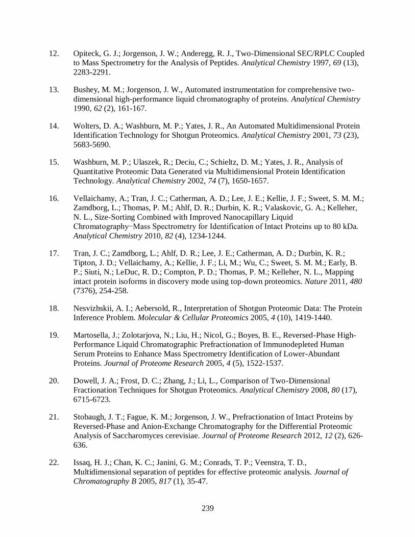
239
12. Opiteck, G. J.; Jorgenson, J. W.; Anderegg, R. J., Two-Dimensional SEC/RPLC Coupled
to Mass Spectrometry for the Analysis of Peptides. Analytical Chemistry 1997, 69 (13),
2283-2291.
13. Bushey, M. M.; Jorgenson, J. W., Automated instrumentation for comprehensive two-
dimensional high-performance liquid chromatography of proteins. Analytical Chemistry
1990, 62 (2), 161-167.
14. Wolters, D. A.; Washburn, M. P.; Yates, J. R., An Automated Multidimensional Protein
Identification Technology for Shotgun Proteomics. Analytical Chemistry 2001, 73 (23),
5683-5690.
15. Washburn, M. P.; Ulaszek, R.; Deciu, C.; Schieltz, D. M.; Yates, J. R., Analysis of
Quantitative Proteomic Data Generated via Multidimensional Protein Identification
Technology. Analytical Chemistry 2002, 74 (7), 1650-1657.
16. Vellaichamy, A.; Tran, J. C.; Catherman, A. D.; Lee, J. E.; Kellie, J. F.; Sweet, S. M. M.;
Zamdborg, L.; Thomas, P. M.; Ahlf, D. R.; Durbin, K. R.; Valaskovic, G. A.; Kelleher,
N. L., Size-Sorting Combined with Improved Nanocapillary Liquid
Chromatography−Mass Spectrometry for Identification of Intact Proteins up to 80 kDa.
Analytical Chemistry 2010, 82 (4), 1234-1244.
17. Tran, J. C.; Zamdborg, L.; Ahlf, D. R.; Lee, J. E.; Catherman, A. D.; Durbin, K. R.;
Tipton, J. D.; Vellaichamy, A.; Kellie, J. F.; Li, M.; Wu, C.; Sweet, S. M. M.; Early, B.
P.; Siuti, N.; LeDuc, R. D.; Compton, P. D.; Thomas, P. M.; Kelleher, N. L., Mapping
intact protein isoforms in discovery mode using top-down proteomics. Nature 2011, 480
(7376), 254-258.
18. Nesvizhskii, A. I.; Aebersold, R., Interpretation of Shotgun Proteomic Data: The Protein
Inference Problem. Molecular & Cellular Proteomics 2005, 4 (10), 1419-1440.
19. Martosella, J.; Zolotarjova, N.; Liu, H.; Nicol, G.; Boyes, B. E., Reversed-Phase High-
Performance Liquid Chromatographic Prefractionation of Immunodepleted Human
Serum Proteins to Enhance Mass Spectrometry Identification of Lower-Abundant
Proteins. Journal of Proteome Research 2005, 4 (5), 1522-1537.
20. Dowell, J. A.; Frost, D. C.; Zhang, J.; Li, L., Comparison of Two-Dimensional
Fractionation Techniques for Shotgun Proteomics. Analytical Chemistry 2008, 80 (17),
6715-6723.
21. Stobaugh, J. T.; Fague, K. M.; Jorgenson, J. W., Prefractionation of Intact Proteins by
Reversed-Phase and Anion-Exchange Chromatography for the Differential Proteomic
Analysis of Saccharomyces cerevisiae. Journal of Proteome Research 2012, 12 (2), 626-
636.
22. Issaq, H. J.; Chan, K. C.; Janini, G. M.; Conrads, T. P.; Veenstra, T. D.,
Multidimensional separation of peptides for effective proteomic analysis. Journal of
Chromatography B 2005, 817 (1), 35-47.

240
23. Fenn, L.; Kliman, M.; Mahsut, A.; Zhao, S.; McLean, J., Characterizing ion mobility-
mass spectrometry conformation space for the analysis of complex biological samples.
Anal Bioanal Chem 2009, 394 (1), 235-244.
24. Hebert, A. S.; Richards, A. L.; Bailey, D. J.; Ulbrich, A.; Coughlin, E. E.; Westphall, M.
S.; Coon, J. J., The One Hour Yeast Proteome. Molecular & Cellular Proteomics 2014,
13 (1), 339-347.
25. Yates, J. R.; Ruse, C. I.; Nakorchevsky, A., Proteomics by Mass Spectrometry:
Approaches, Advances, and Applications. Annual Review of Biomedical Engineering
2009, 11 (1), 49-79.
26. Wilm, M. S.; Mann, M., Electrospray and Taylor-Cone theory, Dole's beam of
macromolecules at last? International Journal of Mass Spectrometry and Ion Processes
1994, 136 (2–3), 167-180.
27. Wilm, M.; Mann, M., Analytical Properties of the Nanoelectrospray Ion Source.
Analytical Chemistry 1996, 68 (1), 1-8.
28. Matzke, M. M.; Brown, J. N.; Gritsenko, M. A.; Metz, T. O.; Pounds, J. G.; Rodland, K.
D.; Shukla, A. K.; Smith, R. D.; Waters, K. M.; McDermott, J. E.; Webb-Robertson, B.-
J., A comparative analysis of computational approaches to relative protein quantification
using peptide peak intensities in label-free LC-MS proteomics experiments.
PROTEOMICS 2013, 13 (3-4), 493-503.
29. Gasch, A. P.; Spellman, P. T.; Kao, C. M.; Carmel-Harel, O.; Eisen, M. B.; Storz, G.;
Botstein, D.; Brown, P. O., Genomic Expression Programs in the Response of Yeast
Cells to Environmental Changes. Molecular Biology of the Cell 2000, 11 (12), 4241-
4257.
30. Searle, B. C., Scaffold: A bioinformatic tool for validating MS/MS-based proteomic
studies. PROTEOMICS 2010, 10 (6), 1265-1269.
31. Eng, J. K.; Searle, B. C.; Clauser, K. R.; Tabb, D. L., A Face in the Crowd: Recognizing
Peptides Through Database Search. Molecular & Cellular Proteomics 2011, 10 (11).
32. Bantscheff, M.; Lemeer, S.; Savitski, M.; Kuster, B., Quantitative mass spectrometry in
proteomics: critical review update from 2007 to the present. Anal Bioanal Chem 2012,
404 (4), 939-965.
33. Raubenheimer, D.; Simpson, S. L., Analysis of covariance: an alternative to nutritional
indices. Entomologia Experimentalis et Applicata 1992, 62 (3), 221-231.
34. Davis, J. M.; Stoll, D. R.; Carr, P. W., Dependence of Effective Peak Capacity in
Comprehensive Two-Dimensional Separations on the Distribution of Peak Capacity
between the Two Dimensions. Analytical Chemistry 2008, 80 (21), 8122-8134.

241
35. Fraenkel, D. G., Carbohydrate metabolism [in yeast]. Cold Spring Harbor Monogr. Ser.
1982, 11B, 1-37.
36. Fernandez, R.; Herrero, P.; Moreno, R., Inhibition and Inactivation of Glucose-
phosphorylating Enzymes from Sacchavomyces cevevisiae by D-Xylose. Microbiology
1895, 131, 2705-2709.
37. Herrero, P.; Galíndez, J.; Ruiz, N.; Martínez-Campa, C.; Moreno, F., Transcriptional
regulation of the Saccharomyces cerevisiae HXK1, HXK2 and GLK1 genes. Yeast 1995,
11 (2), 137-144.
38. Yang, J.; Bae, J. Y.; Lee, Y. M.; Kwon, H.; Moon, H.-Y.; Kang, H. A.; Yee, S.-b.; Kim,
W.; Choi, W., Construction of Saccharomyces cerevisiae strains with enhanced ethanol
tolerance by mutagenesis of the TATA-binding protein gene and identification of novel
genes associated with ethanol tolerance. Biotechnology and Bioengineering 2011, 108
(8), 1776-1787.
39. Castelli, L. M.; Lui, J.; Campbell, S. G.; Rowe, W.; Zeef, L. A. H.; Holmes, L. E. A.;
Hoyle, N. P.; Bone, J.; Selley, J. N.; Sims, P. F. G.; Ashe, M. P., Glucose depletion
inhibits translation initiation via eIF4A loss and subsequent 48S preinitiation complex
accumulation, while the pentose phosphate pathway is coordinately up-regulated.
Molecular Biology of the Cell 2011, 22 (18), 3379-3393.
40. Zampar, G. G.; Kümmel, A.; Ewald, J.; Jol, S.; Niebel, B.; Picotti, P.; Aebersold, R.;
Sauer, U.; Zamboni, N.; Heinemann, M., Temporal system‐level organization of the
switch from glycolytic to gluconeogenic operation in yeast. Molecular Systems Biology
2013, 9 (1).
41. Sprague, G. F.; Cronan, J. E., Isolation and characterization of Saccharomyces cerevisiae
mutants defective in glycerol catabolism. Journal of Bacteriology 1977, 129 (3), 1335-
1342.
42. Grauslund, M.; Lopes, J. M.; Rønnow, B., Expression of GUT1, which encodes glycerol
kinase in Saccharomyces cerevisiae, is controlled by the positive regulators Adr1p, Ino2p
and Ino4p and the negative regulator Opi1p in a carbon source-dependent fashion.
Nucleic Acids Research 1999, 27 (22), 4391-4398.
43. Cronwright, G. R.; Rohwer, J. M.; Prior, B. A., Metabolic Control Analysis of Glycerol
Synthesis in Saccharomyces cerevisiae. Applied and Environmental Microbiology 2002,
68 (9), 4448-4456.
44. ter Schure, E. G.; Flikweert, M. T.; van Dijken, J. P.; Pronk, J. T.; Verrips, C. T.,
Pyruvate Decarboxylase Catalyzes Decarboxylation of Branched-Chain 2-Oxo Acids but
Is Not Essential for Fusel Alcohol Production by Saccharomyces cerevisiae. Applied and
Environmental Microbiology 1998, 64 (4), 1303-1307.
45. Brewster, N. K.; Val, D. L.; Walker, M. E.; Wallace, J. C., Regulation of Pyruvate
Carboxylase Isozyme (PYC1, PYC2) Gene Expression in Saccharomyces cerevisiae

242
during Fermentative and Nonfermentative Growth. Archives of Biochemistry and
Biophysics 1994, 311 (1), 62-71.
46. Pavlik, P.; Simon, M.; Schuster, T.; Ruis, H., The glycerol kinase (GUT1 ) gene of
Saccharomyces cerevisiae cloning and characterization. Current Genetics 1993, 24 (1),
21-25.
47. Blumberg, H.; Hartshorne, T. A.; Young, E. T., Regulation of expression and activity of
the yeast transcription factor ADR1. Molecular and Cellular Biology 1988, 8 (5), 1868-
1876.
48. Kratzer, S.; Schüller, H.-J., Transcriptional control of the yeast acetyl-CoA synthetase
gene, ACS1, by the positive regulators CAT8 and ADR1 and the pleiotropic repressor
UME6. Molecular Microbiology 1997, 26 (4), 631-641.
49. Simon, M.; Binder, M.; Adam, G.; Hartig, A.; Ruis, H., Control of peroxisome
proliferation in Saccharomyces cerevisiae by ADR1, SNF1 (CAT1, CCR1) and SNF4
(CAT3). Yeast 1992, 8 (4), 303-309.
50. Wang, X.; Mann, C. J.; Bai, Y.; Ni, L.; Weiner, H., Molecular Cloning, Characterization,
and Potential Roles of Cytosolic and Mitochondrial Aldehyde Dehydrogenases in Ethanol
Metabolism in Saccharomyces cerevisiae. Journal of Bacteriology 1998, 180 (4), 822-
830.
51. Van Den Berg, M. A.; Steensma, H. Y., ACS2, a Saccharomyces Cerevisiae Gene
Encoding Acetyl-Coenzyme A Synthetase, Essential for Growth on Glucose. European
Journal of Biochemistry 1995, 231 (3), 704-713.
52. Takahashi, H.; McCaffery, J. M.; Irizarry, R. A.; Boeke, J. D., Nucleocytosolic Acetyl-
Coenzyme A Synthetase Is Required for Histone Acetylation and Global Transcription.
Molecular Cell 2006, 23 (2), 207-217.
53. Moldave, K., Progress in Nucleic Acid Research and Molecular Biology. Elsevier
Science: 1997.

243
APPENDIX A. SUPPLEMENTAL DATA FOR CHAPTER 2
Appendix A.1. To compare the 10 equal-mass and 10 equal-time fractions, the Normalized
Difference Protein Coverage (NDPC) was plotted with proteins with higher coverage on the left,
and proteins with lower coverage on the right. If a protein was identified with higher sequence
coverage in the 10 equal-mass fractions, its NDPC value was positive (red bars). The blue bars
signified higher coverage in the 10 equal-time fractions. Differences in coverage were minimal
for highly covered proteins. As protein coverage decreased, more proteins were identified with
higher coverage in the equal-mass fractions. The dashed lines indicate a level of two-fold greater
protein coverage.
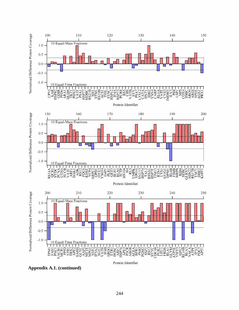
244
Appendix A.1. (continued)

245
Appendix A.1. (continued)

246
Appendix A.2. To compare the 20 equal-mass and 20 equal-time fractions, the Normalized
Difference Protein Coverage (NDPC) was plotted with proteins with higher coverage on the left,
and proteins with lower coverage on the right. If a protein was identified with higher sequence
coverage in the 20 equal-mass fractions, its NDPC value was positive (red bars). The blue bars
signified higher coverage in the 20 equal-time fractions. Differences in coverage were minimal
for highly covered proteins. For 20 fractions, the NDPC did not favor the equal-mass or the
equal-time fractionation methods. The dashed lines indicate a level of two-fold greater protein
coverage.

247
Appendix A.2. (continued)

248
Appendix A.2. (continued)

249
Appendix A.2. (continued)

250
Appendix A.2. (continued)

251
APPENDIX B. SUPPLEMENTAL DATA FOR CHAPTER 3
Appendix B.1. The NDPC comparing the analysis on the 98.2 cm column run at 30 kpsi to the
44.1 cm column run at 15 kpsi for a 90 min gradient was plotted for each protein identified in an
E. coli digest standard. If a protein was identified with higher sequence coverage with the
separation on the 98.2 cm column, its NDPC value was positive (blue bars). The red bars
signified higher coverage with the separation on the 44.1 cm column. Proteins with higher
coverage were plotted on the left, and proteins with lower coverage were on the right.
Differences in coverage were minimal for highly covered proteins. As protein coverage
decreased, more proteins were identified with higher coverage with the separation on the 98.2 cm
column. The dashed line represented a two-fold difference in protein coverage.

252
Appendix B.1. (continued)

253
Appendix B.1. (continued)

254
Appendix B.2. The NDPC comparing the analysis on the 98.2 cm column run at 30 kpsi to the
44.1 cm column run at 15 kpsi for a 180 min gradient was plotted for each protein identified in
an E. coli digest standard. If a protein was identified with higher sequence coverage with the
separation on the 98.2 cm column, its NDPC value was positive (blue bars). The red bars
signified higher coverage with the separation on the 44.1 cm column. Proteins with higher
coverage were plotted on the left, and proteins with lower coverage were on the right.
Differences in coverage were minimal for highly covered proteins. As protein coverage
decreased, more proteins were identified with higher coverage with the separation on the 98.2 cm
column. The dashed line represented a two-fold difference in protein coverage.
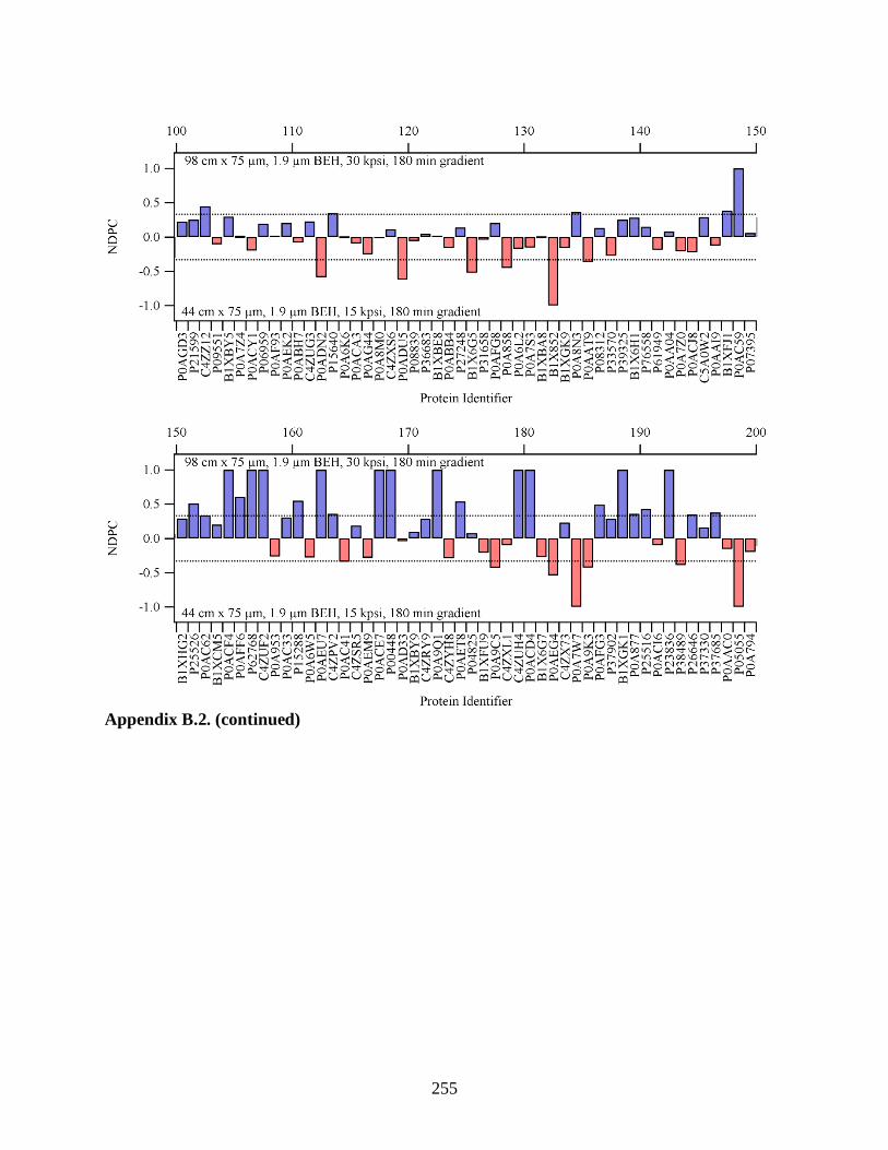
255
Appendix B.2. (continued)

256
Appendix B.2. (continued)

257
Appendix B.3. Chromatograms of MassPREPTM
Digestion Standard Protein Expression Mixture
2 were collected for separations with increasing pressure and flow rate on the 39.2 cm x 75 µm
ID column packed with 1.4 µm BEH C18 particles. Separations were completed with a 50µL
gradient volume. The insert of a representative peptide peak with 724 m/z extracted from all
three chromatograms showed the decrease in peak width and constant signal intensity as pressure
and flow rate increased.
1000
800
600
400
200
0
BP
I
200150100500
Time (min)
4-40 %B at 65°C, 50 µL
1% Change MPB / Column Volume
39.2 cm x 75 µm ID, 1.4 µm BEH C18
15 kpsi, 190 nL/min
30 kpsi, 410 nL/min
45 kpsi, 610 nL/min
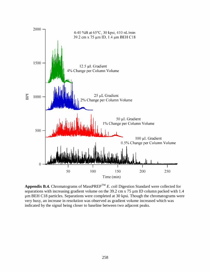
258
Appendix B.4. Chromatograms of MassPREPTM
E. coli Digestion Standard were collected for
separations with increasing gradient volume on the 39.2 cm x 75 µm ID column packed with 1.4
µm BEH C18 particles. Separations were completed at 30 kpsi. Though the chromatograms were
very busy, an increase in resolution was observed as gradient volume increased which was
indicated by the signal being closer to baseline between two adjacent peaks.

259
Appendix B.5. Chromatograms of MassPREPTM
E. coli Digestion Standard were collected for
separations with increasing pressure and flow rate on the 39.2 cm x 75 µm ID column packed
with 1.4 µm BEH C18 particles. Separations were completed with a 50µL gradient volume.
1200
1000
800
600
400
200
0
BP
I
200150100500
Time (min)
4-40 %B at 65°C, 50 µL
1% Change MPB / Column Volume
39.2 cm x 75 µm ID, 1.4 µm BEH C18
15 kpsi, 190 nL/min
30 kpsi, 410 nL/min
45 kpsi, 610 nL/min

260
APPENDIX C. SUPPLEMENTAL DATA FOR CHAPTER 5
Appendix C.1. To compare the 10 fractions run on the modified system to the 10 fractions run
on the standard UPLC, the NDPC is plotted with proteins with higher coverage on the left, and
proteins with lower coverage on the right. If a protein was identified with higher sequence
coverage when analyzed on the modified UHPLC, its NDPC value is positive (blue bars). The
red bars signify higher coverage in the analysis on the standard UPLC. Differences in coverage
were minimal for highly covered proteins. As protein coverage decreased, more proteins were
identified with higher coverage from the analysis on the modified UHPLC. The dashed lines
indicate a level of two-fold greater protein coverage. (This was a large graph and split into
multiple parts.)

261
Appendix C.1. (continued)

262
Appendix C.1. (continued)
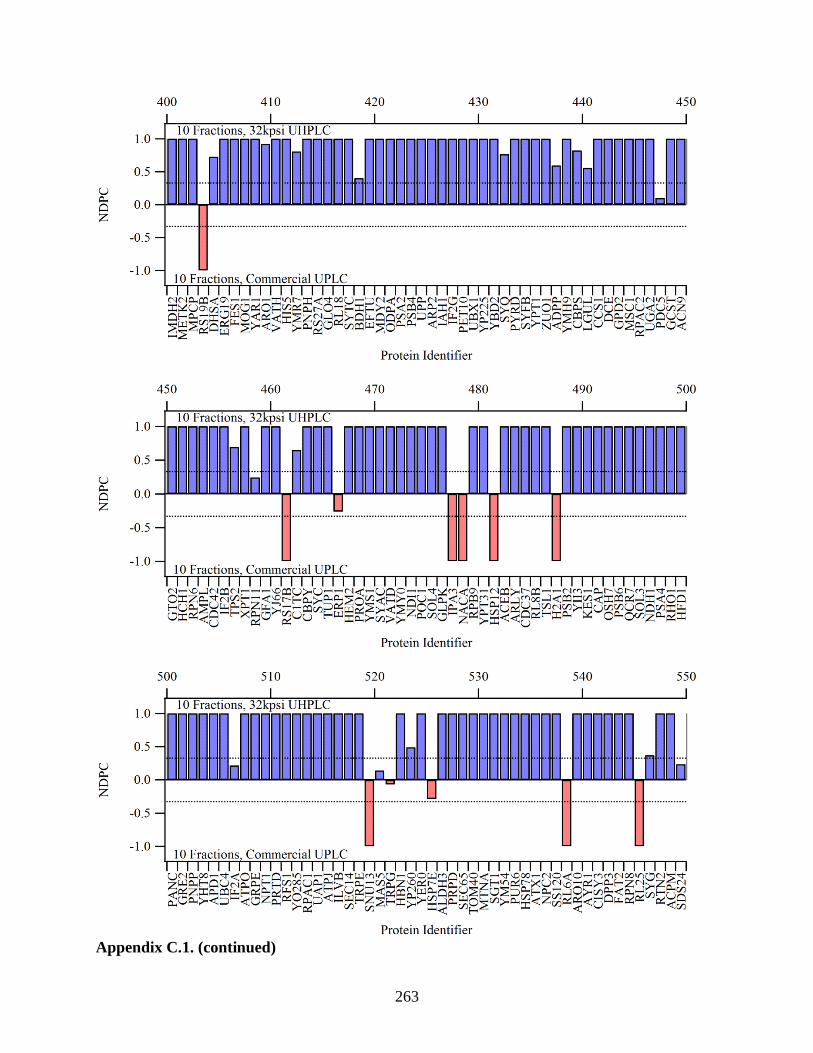
263
Appendix C.1. (continued)

264
Appendix C.1. (continued)
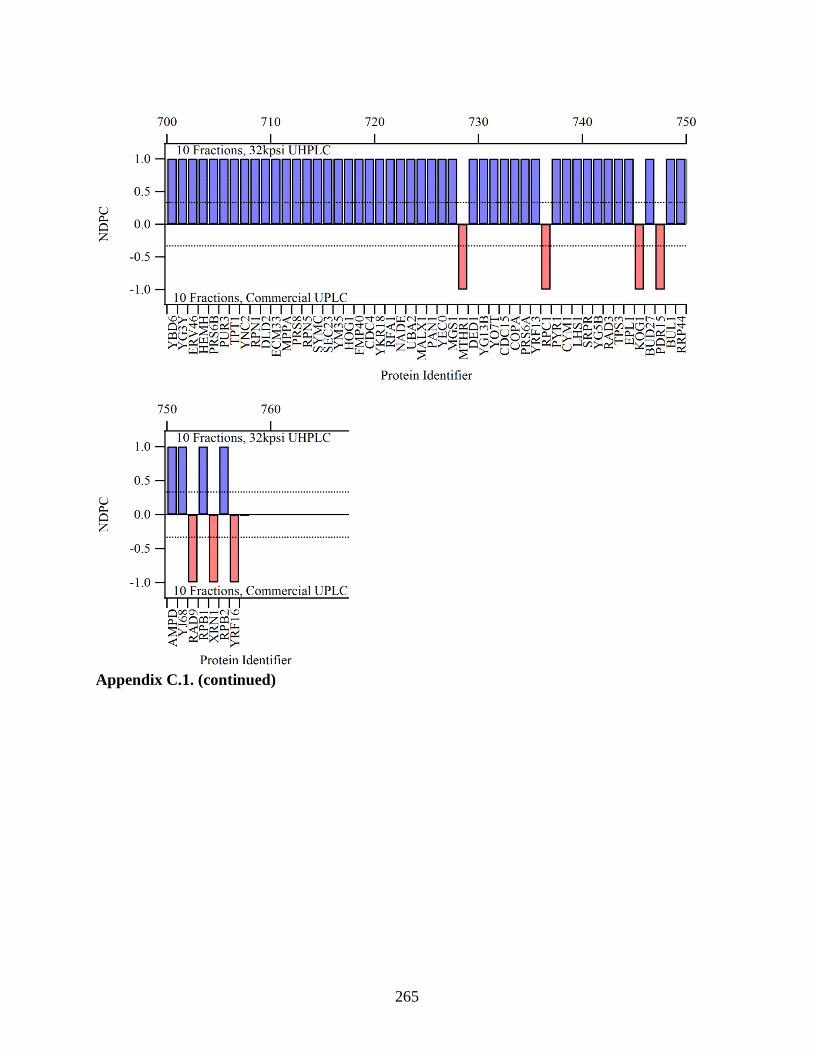
265
Appendix C.1. (continued)

266
Appendix C.2. To compare the 20 fractions run on the modified system to the 20 fractions run
on the standard UPLC, the NDPC is plotted with proteins with higher coverage on the left, and
proteins with lower coverage on the right. If a protein was identified with higher sequence
coverage when analyzed on the modified UHPLC, its NDPC value is positive (blue bars). The
red bars signify higher coverage in the analysis on the standard UPLC. Differences in coverage
were minimal for highly covered proteins. As protein coverage decreased, more proteins were
identified with higher coverage from the analysis on the modified UHPLC. The dashed lines
indicate a level of two-fold greater protein coverage. (This was a large graph and split into
multiple parts.)

267
Appendix C.2. (Continued)

268
Appendix C.2. (Continued)

269
Appendix C.2. (Continued)

270
Appendix C.2. (Continued)

271
Appendix C.2. (Continued)
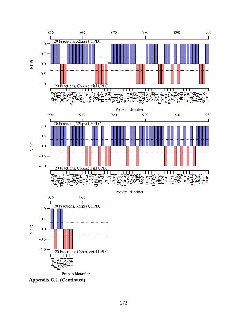
272
Appendix C.2. (Continued)
Related Documents