Multicomponent reactive transport modeling of uranium bioremediation field experiments

Ž .Journal of Contaminant Hydrology 52 2001 85–108www.elsevier.comrlocaterjconhyd

Multi-component reactive transport modeling ofnatural attenuation of an acid groundwater plume at

a uranium mill tailings site

Chen Zhu a,), Fang Q. Hu a, David S. Burden b

a Old Dominion UniÕersity, Norfolk, VA 23529, USAb U.S. EnÕironmental Protection Agency, National Risk Management Research Laboratory,

Ada, OK 74820, USA

Received 10 December 1999; received in revised form 7 April 2000; accepted 20 April 2000

Abstract

Natural attenuation of an acidic plume in the aquifer underneath a uranium mill tailings pondin Wyoming, USA was simulated using the multi-component reactive transport code PHREEQC. Aone-dimensional model was constructed for the site and the model included advective–dispersivetransport, aqueous speciation of 11 components, and precipitation–dissolution of six minerals.Transport simulation was performed for a reclamation scenario in which the source of acidicseepage will be terminated after 5 years and the plume will then be flushed by uncontaminatedupgradient groundwater. Simulations show that successive pH buffer reactions with calcite,Ž . Ž . Ž . Ž .Al OH a , and Fe OH a create distinct geochemical zones and most reactions occur at the3 3

boundaries of geochemical zones. The complex interplay of physical transport processes andchemical reactions produce multiple concentration waves. For SO2y transport, the concentration4

waves are related to advection–dispersion, and gypsum precipitation and dissolution. Wave speedsfrom numerical simulations compare well to an analytical solution for wave propagation. q 2001Elsevier Science B.V. All rights reserved.

Keywords: Geochemical modeling; Contaminant; Transport; Coupled processes

1. Introduction

Accurate prediction of the fate and transport of regulated metals and radionuclides inthe subsurface of abandoned mining sites is critical to the assessment of environmental

) Corresponding author. Present address: Department of Geology and Planetary Science, University ofPittsburg, Pittsburg, PA 15260. Tel.: q1-412-624-8780.

Ž .E-mail address: [email protected] C. Zhu .

0169-7722r01r$ - see front matter q2001 Elsevier Science B.V. All rights reserved.Ž .PII: S0169-7722 01 00154-1

( )C. Zhu et al.rJournal of Contaminant Hydrology 52 2001 85–10886

impact and to the development of effective remediation technologies. However, this taskhas been almost exclusively addressed, in industrial practice, by the use of K -basedd

AreactiveB transport models. K or linear isotherm, as well as Langmuir and Freundlichd

isotherms, are phenomenological and empirical parameters. Although K -based trans-d

port models are mathematically simple, it is well known that they are insufficient todescribe the complex geochemical reactions that control the distribution of solutes

Žbetween groundwater and aquifer matrix in subsurface environments Stumm and.Morgan, 1981; Reardon, 1981; Bethke and Brady, 2000 . In the case of active or

abandoned mining sites with acid mine drainage problems, the shortcomings of thisapproach become more severe because

Ž .1 Precipitation–dissolution reactions dominate the attenuation of some solutes.Because the solubility products control the reactions but the mass of the solids plays nopart in the solubility product constraints, no continuously differentiable isotherms relate

Žsolid and fluid concentrations for precipitation–dissolution reactions Bryant et al.,.1987 ;

Ž .2 The single retardation factor approach fails to consider the interactions amongmultiple solutes. These interactions are important in the transport of some contaminants.For example, the precipitation of gypsum, which retards the transport of sulfate ingroundwater in acid mine drainage systems, results from the rise of the activity ofcalcium in groundwater due to calcite dissolution. Calcite dissolution is in turn a resultof the transport of protons;

Ž .3 The seepage of acidic fluid into even a homogenous aquifer will producechemical zonations or heterogeneity, which also evolves spatially through time. Thus, itis impossible to have a constant K or to know the variation of K values with timed d

and space a priori.A more promising approach to the simulation of reactions and flow in chemically

complex and heterogeneous environments is the use of coupled reactiÕe transportmodels in which the advective–dispersive transport equations are solved together, eithersimultaneously or sequentially, with the mass-action and mass-balance equations for

Žchemical reactions Schwartz and Domenico, 1973; Walsh, 1983; Cederberg et al., 1985;Lichtner, 1985; Yeh and Tripathi, 1989, 1991; Steefel and Lasaga, 1994; Raffensperger

.and Garven, 1995 . Dozens of coupled reactive transport models have been developed inŽ .the past 20 years see reviews by Mangold and Tsang, 1991; Zhu et al., 1996 . However,

applications of coupled reactive transport models to abandoned mining sites are scarce.Ž .Yeh and Tripathi 1991 applied the model HYDROGEOCHEM to a AsyntheticB uranium

Ž .mill-tailings site and incorporated limited chemistry. Walter et al. 1994b appliedMINTRAN to a AgenericB abandoned mining site, resembling the Nordic mine uranium

Ž .mill tailings site near Elliot Lake, Northern Ontario. Glynn and Brown 1996 describedpreliminary results of application of the PHREEQC model to the Pinal Creek site in

Ž .Arizona. Despite the seriousness of the acid mine drainage problem cf. King, 1995 , thechemical reactions and chemical evolution in the aquifers as a result of seepage of acidicfluids are poorly understood.

In this study, natural attenuation of a contaminated aquifer in an abandoned uraniummill tailings site in Wyoming, USA was simulated using the U.S. Geological Survey

Žmulti-component reactive transport code PHREEQC version 2.0 Parkhurst and Appello,

( )C. Zhu et al.rJournal of Contaminant Hydrology 52 2001 85–108 87

. Ž .1999 . A recent study of this site the Bear Creek Uranium site has collected a largeŽ .amount of hydrological and geochemical data Zhu et al., 2001 . This study thus allows

the development of a more complex and detailed reactive transport model than possiblein previous studies. Modeling results were qualitatively compared to field data andanalyzed in terms of concentration wave propagation.

2. Site contamination and hydrogeological setting

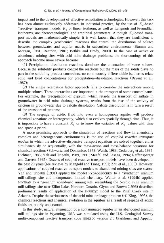
The Bear Creek Uranium site is located in the southern part of the Powder RiverŽ .Basin in Wyoming Fig. 1 . A uranium mill operated from the 1970s to the mid-1980s.

Sulfuric acid and sodium chlorate were used to dissolve and oxidize uranium. Spentacids and tailings slurries were piped to unlined tailings ponds. An estimated 3.3 milliontons of tailings and 880 million gallons of liquid effluent have been disposed into the

Fig. 1. Plan view of the mine site and tailings impoundment. The dashed lines are pH contours, whichdelineate the flow paths at the site.


tailings pond. The tailings fluid has a pH between 1.5 and 3.5, a total dissolved solidŽ . Ž .TDS content close to 20,000 mgrl, and high concentrations of arsenic As , berylliumŽ . Ž . Ž . Ž . Ž . Ž .Be , cadmium Cd , chromium Cr , lead Pb , molybdenum Mo , nickel Ni ,

Ž . Ž226 228 . Ž230 . Ž .selenium Se , radium Ra, Ra , thorium Th , and uranium U .Seepage from the disposal ponds into the underlying N sand of the Eocene Upper

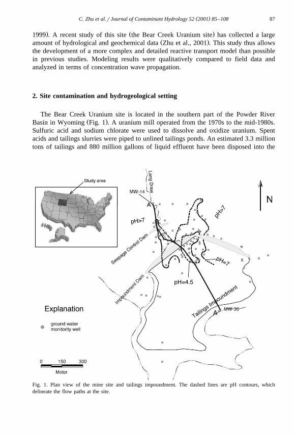
Ž .Wasatch Formation and alluvium aquifer has formed an acid plume Fig. 2 . The N sandand alluvium at the site is comprised primarily of quartz, microcline, a small amount of

Ž .plagioclase, and about 2 wt.% calcite Sharp and Gibbons, 1964; Zhu et al., 2001 .Measured total iron concentration in the Wasatch Formation is about 0.4 wt.% as FeŽ .Sharp and Gibbons, 1964 . Groundwater occurs 3 to 8 m below land surface. Numerousaquifer tests have been performed to evaluate transmissivities and storage coefficients.The hydraulic conductivity for the alluvium at Lang Draw is estimated at 3 mrday and

Žfor N sand beneath the tailings impoundments is 0.9 mrday GeoTrans, 1987, 1995,.unpublished reports . A groundwater flow model was developed and modeling results

show that groundwater flows preferentially in the alluvium along Lang Draw, where thepermeability is high, and to the northeast from the bend of the Impoundment DamŽ .GeoTrans, 1987, 1995, unpublished reports . These flow paths are supported by

Ž .groundwater pH data, which outline the plume of lower pH groundwater Fig. 1 .Regional groundwater flows from the south of the site beneath the tailings basin and tothe north. The estimated pre-mining regional groundwater gradient is 0.014 mrm.

To contain the migration of the plume downgradient, low-pH water was pumpedfrom wells installed along the Lang Draw downgradient from the impoundment dam andpiped into constructed evaporation basins within the tailings impoundment. Over time,the efficiency of these pumping wells has decreased significantly. The current reclama-tion plan is to install a low-permeability cover on the tailings ponds to prevent furtherinfiltration from precipitation. Results from hydrological modeling show that tailings

Fig. 2. Cross-section A–AX from Fig. 1. It also shows the names and locations of the monitoring wellsdiscussed in the text. Shaded area in the aquifer represents the estimated extent of the low-pH plume.


pore water will cease to drain into the underlying N sand 5 years after the coverinstallation. After that time, the plume will be flushed by uncontaminated upgradientgroundwater. The distance of the migration of the acid plume and regulated metals andradionuclides will depend on the Anatural attenuationB or the reactions of aquiferminerals with contaminated groundwater. The coupled reactive transport model isdesigned to simulate the acid plume migration under this Acover and attenuateBreclamation plan.

3. Model description

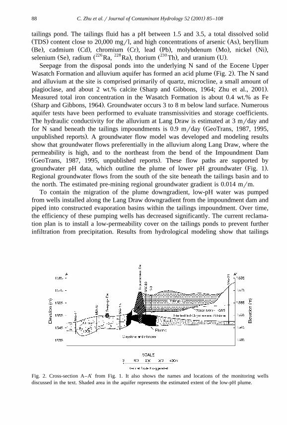
X Ž . ŽAn 800-m strip along cross-section A–A Fig. 2 was discretized into 200 cells Fig..3 . Each cell is 4 m in length. The model starts at the southern end of the pH 4.5 zone in

the N sand and extends to near the property boundary. Grid size sensitivity analysis wasperformed by varying the grid size from 1 to 10 m, while keeping other parameters the

Ž .same time steps also changed accordingly . The results from these simulations showthat the differences are indiscernible. For the base case, the time step is 0.08 year.

A uniform and constant Darcy velocity of 15 mryear and effective porosity of 0.3were used along the entire cross-section. The tailings fluid has high chloride concentra-

Ž .tions 0.016 molrl , while the background water has only 0.0007 molrl. It is widelybelieved that Cly acts as a conservative solute in most aquifer systems and thus, itsdistribution can be used to retrieve dispersivity for the aquifer. By trial and error, alongitudinal dispersivity between 10 and 15 m appears to fit the concentration differ-ences best in monitor wells sampled in September 1994. It is assumed in this study thatmolecular diffusion is negligible with respect to advection and dispersion.

Ž .From field data and speciation-solubility modeling, Zhu et al. 2001 concluded thatthe distinct geochemistry zones in the aquifer could be interpreted with successive pH

Ž . Ž .buffer reactions with calcite, amorphous Al OH , and amorphous Fe OH . This3 3

conceptual model was used as a geochemical submodel for the coupled reactivetransport. A total of 11 aqueous components, H, Ca, Mg, Cl, CO2y, Al, SO2y, Fe3q,3 4

Ž . Ž . Ž . Ž . Ž .Na, K, and Si, and six minerals, Al OH a , Fe OH a , calcite, gypsum, SiO a , and3 3 2

illite, were included in the simulations. Equilibrium constants for chemical reactions arelisted in Table 1. For simplicity, chemical reactions were calculated at 25 8C and 1 baralthough measured groundwater temperatures range from 12 to 16 8C. The local

Ž .equilibrium assumption LEA is used.

Fig. 3. Discretization of the simulated domain.


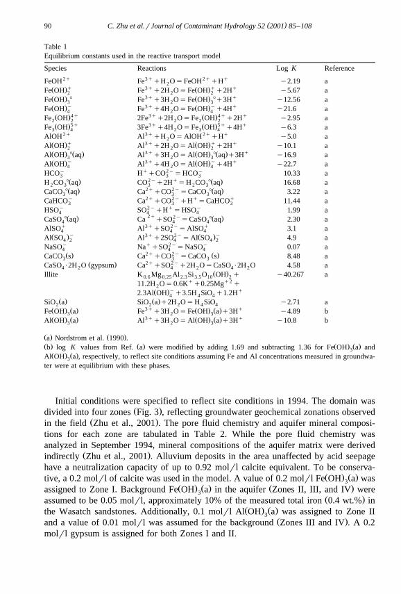
Table 1Equilibrium constants used in the reactive transport model

Species Reactions Log K Reference2q 3q 2q qFeOH Fe qH OsFeOH qH y2.19 a2q 3q q qŽ . Ž .Fe OH Fe q2H OsFe OH q2H y5.67 a2 2 2

3q qŽ . Ž .Fe OH 8 Fe q3H OsFe OH 8q3H y12.56 a3 2 3y 3q y qŽ . Ž .Fe OH Fe q4H OsFe OH q4H y21.6 a4 2 4

4q 3q 4q qŽ . Ž .Fe OH 2Fe q2H OsFe OH q2H y2.95 a2 2 2 2 25q 3q 5q qŽ . Ž .Fe OH 3Fe q4H OsFe OH q4H y6.3 a3 4 2 3 4

2q 3q 2q qAlOH Al qH OsAlOH qH y5.0 a2q 3q q qŽ . Ž .Al OH Al q2H OsAl OH q2H y10.1 a2 2 2

3q qŽ . Ž . Ž . Ž .Al OH 8 aq Al q3H OsAl OH 8 aq q3H y16.9 a3 2 3y 3q y qŽ . Ž .Al OH Al q4H OsAl OH q4H y22.7 a4 2 4

y q 2y yHCO H qCO sHCO 10.33 a3 3 32y qŽ . Ž .H CO 8 aq CO q2H sH CO 8 aq 16.68 a2 3 3 2 3

2q 2yŽ . Ž .CaCO 8 aq Ca qCO sCaCO 8 aq 3.22 a3 3 3y 2q 2y q qCaHCO Ca qCO qH sCaHCO 11.44 a3 3 3

y 2y q yHSO SO qH sHSO 1.99 a4 4 42q 2yŽ . Ž .CaSO 8 aq Ca qSO sCaSO 8 aq 2.30 a4 4 4

q 3q 2y qAlSO Al qSO sAlSO 3.1 a4 4 4y 3q 2y yŽ . Ž .Al SO Al q2SO sAl SO 4.9 a4 2 4 4 2

y q 2y yNaSO Na qSO sNaSO 0.07 a4 4 42q 2yŽ . Ž .CaCO s Ca qCO sCaCO s 8.48 a3 3 32q 2yŽ .CaSO P2H O gypsum Ca qSO q2H OsCaSO P2H O 4.58 a4 2 4 2 4 2

Ž .Illite K Mg Al Si O OH q y40.267 a0.6 0.25 2.3 3.5 10 2q q211.2H Os0.6K q0.25Mg q2

y qŽ .2.3Al OH q3.5H SiO q1.2H4 4 4Ž . Ž .SiO a SiO a q2H OsH SiO y2.71 a2 2 2 4 4

3q qŽ . Ž . Ž . Ž .Fe OH a Fe q3H OsFe OH a q3H y4.89 b3 2 33q qŽ . Ž . Ž . Ž .Al OH a Al q3H OsAl OH a q3H y10.8 b3 2 3

Ž . Ž .a Nordstrom et al. 1990 .Ž . Ž . Ž . Ž .b log K values from Ref. a were modified by adding 1.69 and subtracting 1.36 for Fe OH a and3Ž . Ž .Al OH a , respectively, to reflect site conditions assuming Fe and Al concentrations measured in groundwa-3

ter were at equilibrium with these phases.

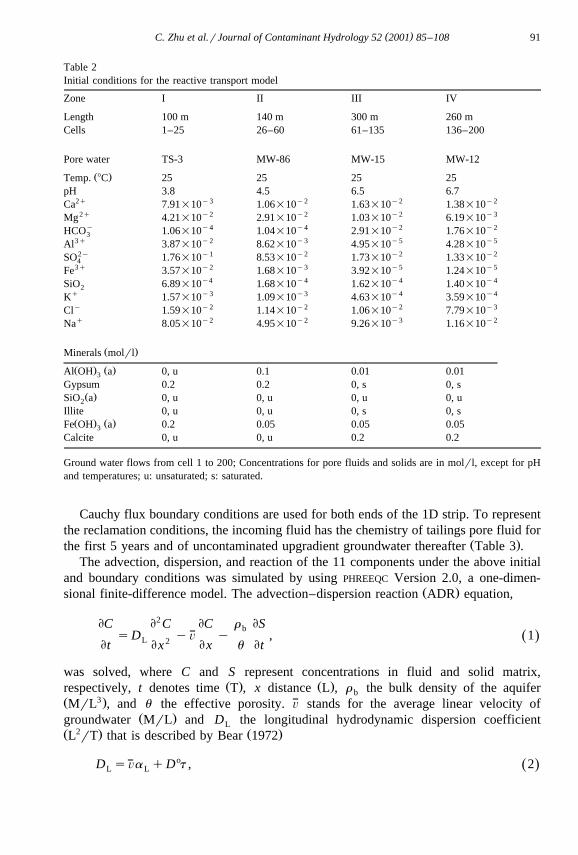
Initial conditions were specified to reflect site conditions in 1994. The domain wasŽ .divided into four zones Fig. 3 , reflecting groundwater geochemical zonations observed

Ž .in the field Zhu et al., 2001 . The pore fluid chemistry and aquifer mineral composi-tions for each zone are tabulated in Table 2. While the pore fluid chemistry wasanalyzed in September 1994, mineral compositions of the aquifer matrix were derived

Ž .indirectly Zhu et al., 2001 . Alluvium deposits in the area unaffected by acid seepagehave a neutralization capacity of up to 0.92 molrl calcite equivalent. To be conserva-

Ž . Ž .tive, a 0.2 molrl of calcite was used in the model. A value of 0.2 molrl Fe OH a was3Ž . Ž . Ž .assigned to Zone I. Background Fe OH a in the aquifer Zones II, III, and IV were3

Ž .assumed to be 0.05 molrl, approximately 10% of the measured total iron 0.4 wt.% inŽ . Ž .the Wasatch sandstones. Additionally, 0.1 molrl Al OH a was assigned to Zone II3

Ž .and a value of 0.01 molrl was assumed for the background Zones III and IV . A 0.2molrl gypsum is assigned for both Zones I and II.


Table 2Initial conditions for the reactive transport model

Zone I II III IV

Length 100 m 140 m 300 m 260 mCells 1–25 26–60 61–135 136–200

Pore water TS-3 MW-86 MW-15 MW-12

Ž .Temp. 8C 25 25 25 25pH 3.8 4.5 6.5 6.7

2q y3 y2 y2 y2Ca 7.91=10 1.06=10 1.63=10 1.38=102q y2 y2 y2 y3Mg 4.21=10 2.91=10 1.03=10 6.19=10y y4 y4 y2 y2HCO 1.06=10 1.04=10 2.91=10 1.76=103

3q y2 y3 y5 y5Al 3.87=10 8.62=10 4.95=10 4.28=102y y1 y2 y2 y2SO 1.76=10 8.53=10 1.73=10 1.33=104

3q y2 y3 y5 y5Fe 3.57=10 1.68=10 3.92=10 1.24=10y4 y4 y4 y4SiO 6.89=10 1.68=10 1.62=10 1.40=102

q y3 y3 y4 y4K 1.57=10 1.09=10 4.63=10 3.59=10y y2 y2 y2 y3Cl 1.59=10 1.14=10 1.06=10 7.79=10q y2 y2 y3 y2Na 8.05=10 4.95=10 9.26=10 1.16=10

Ž .Minerals molrl

Ž . Ž .Al OH a 0, u 0.1 0.01 0.013

Gypsum 0.2 0.2 0, s 0, sŽ .SiO a 0, u 0, u 0, u 0, u2

Illite 0, u 0, u 0, s 0, sŽ . Ž .Fe OH a 0.2 0.05 0.05 0.053

Calcite 0, u 0, u 0.2 0.2

Ground water flows from cell 1 to 200; Concentrations for pore fluids and solids are in molrl, except for pHand temperatures; u: unsaturated; s: saturated.

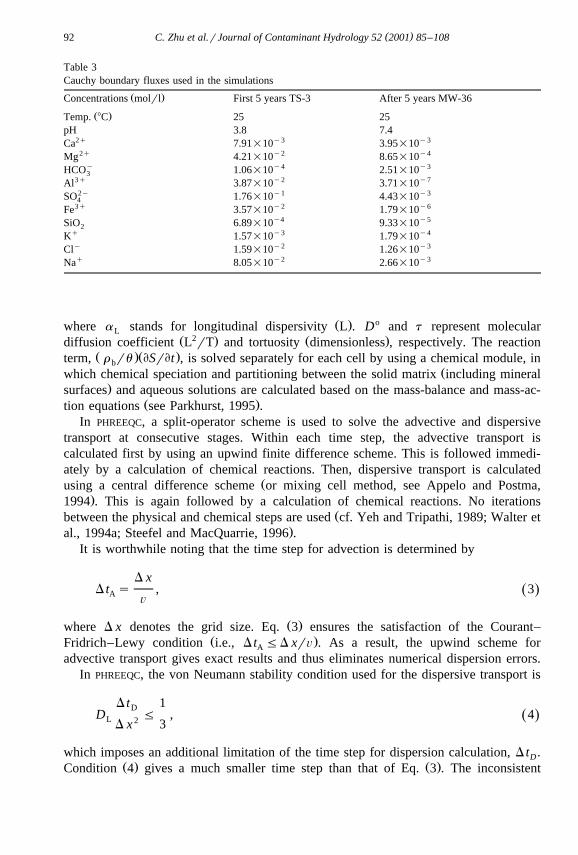
Cauchy flux boundary conditions are used for both ends of the 1D strip. To representthe reclamation conditions, the incoming fluid has the chemistry of tailings pore fluid for

Ž .the first 5 years and of uncontaminated upgradient groundwater thereafter Table 3 .The advection, dispersion, and reaction of the 11 components under the above initial

and boundary conditions was simulated by using PHREEQC Version 2.0, a one-dimen-Ž .sional finite-difference model. The advection–dispersion reaction ADR equation,

EC E2 C EC r ESbsD yÕ y , 1Ž .L 2Et Ex u EtEx

was solved, where C and S represent concentrations in fluid and solid matrix,Ž . Ž .respectively, t denotes time T , x distance L , r the bulk density of the aquiferb

3Ž .MrL , and u the effective porosity. Õ stands for the average linear velocity ofŽ .groundwater MrL and D the longitudinal hydrodynamic dispersion coefficientL

Ž 2 . Ž .L rT that is described by Bear 1972

oD sÕa qD t , 2Ž .L L


Table 3Cauchy boundary fluxes used in the simulations

Ž .Concentrations molrl First 5 years TS-3 After 5 years MW-36

Ž .Temp. 8C 25 25pH 3.8 7.4

2q y3 y3Ca 7.91=10 3.95=102q y2 y4Mg 4.21=10 8.65=10y y4 y3HCO 1.06=10 2.51=103

3q y2 y7Al 3.87=10 3.71=102y y1 y3SO 1.76=10 4.43=104

3q y2 y6Fe 3.57=10 1.79=10y4 y5SiO 6.89=10 9.33=102

q y3 y4K 1.57=10 1.79=10y y2 y3Cl 1.59=10 1.26=10q y2 y3Na 8.05=10 2.66=10

Ž . owhere a stands for longitudinal dispersivity L . D and t represent molecularLŽ 2 . Ž .diffusion coefficient L rT and tortuosity dimensionless , respectively. The reaction

Ž .Ž .term, r ru ESrEt , is solved separately for each cell by using a chemical module, inbŽwhich chemical speciation and partitioning between the solid matrix including mineral

.surfaces and aqueous solutions are calculated based on the mass-balance and mass-ac-Ž .tion equations see Parkhurst, 1995 .

In PHREEQC, a split-operator scheme is used to solve the advective and dispersivetransport at consecutive stages. Within each time step, the advective transport iscalculated first by using an upwind finite difference scheme. This is followed immedi-ately by a calculation of chemical reactions. Then, dispersive transport is calculated

Žusing a central difference scheme or mixing cell method, see Appelo and Postma,.1994 . This is again followed by a calculation of chemical reactions. No iterations

Žbetween the physical and chemical steps are used cf. Yeh and Tripathi, 1989; Walter et.al., 1994a; Steefel and MacQuarrie, 1996 .

It is worthwhile noting that the time step for advection is determined by

D xD t s , 3Ž .A

Õ

Ž .where D x denotes the grid size. Eq. 3 ensures the satisfaction of the Courant–Ž .Fridrich–Lewy condition i.e., D t FD xrÕ . As a result, the upwind scheme forA

advective transport gives exact results and thus eliminates numerical dispersion errors.In PHREEQC, the von Neumann stability condition used for the dispersive transport is

D t 1DD F , 4Ž .L 2 3D x

which imposes an additional limitation of the time step for dispersion calculation, D t .DŽ . Ž .Condition 4 gives a much smaller time step than that of Eq. 3 . The inconsistent


Ž . Ž .requirements by Eqs. 3 and 4 are resolved by using smaller time steps for dispersioncalculations, so that

D tAD t s , 5Ž .D N

where N is an integer. Each of the N dispersion calculations is followed by chemicalreaction calculations.

4. Analysis and discussion of numerical results

Simulations of reactive transport were performed for a period of 5 years of seepageby tailings fluids into the aquifer and 200 years of flushing of the plume by uncontami-nated upgradient groundwater. Because this is a forward model, the modeling results arepredictions of the future and cannot be compared to field data per se. However, for theseepage period, contamination of the aquifer is a continuation of the past and the samegeochemical zonation progresses downgradient. Therefore, the simulated reaction se-quence and concentration levels, although not associated with the spatial and temporalinformation, can be compared to field data. The observed solute concentrations and

Ždistributions have been analyzed using batch-scale geochemical modeling Zhu et al.,.2001 . It is useful to compare them to the results of a model that incorporates transport.

For the flushing period, there are no field data available for comparison presently, butmodeling results can be compared to field data collected in the future.

4.1. Seepage of tailings fluids

The seepage of acidic tailings fluid into the shallow contaminated aquifer causescontinued development of geochemical zonations corresponding to the successive buffer

Ž . Ž . Ž . Ž .reactions with calcite, Al OH a , and Fe OH a . The pH of groundwater is buffered3 3

to 6.3, 4.3, and 3.8, respectively. The reaction

CaCO qSO2yqHqq2H OsCaSO P2H OqHCOy, 6Ž .3 4 2 4 2 3

has a log K value of 6.33 at 25 8C and 1 bar. The buffered pH value by this reaction isdetermined by the ratios of the activity of HCOy and SO2y,3 4

a yHCO 3pHs log K y log . 7Ž .10 ž /2yaSO 4

At the calcite dissolution front, activities of HCOy and SO2y are close to being equal,3 4

and, hence, the pH is buffered to 6.3.The reaction,

Al OH a q3HqsAl3qq3H O, 8Ž . Ž . Ž .3 2

buffers groundwater pH to about 4.3 and the reaction,

Fe3qq3H OsFe OH a q3Hq, 9Ž . Ž . Ž .32


controls groundwater pH to about 3.8. The reaction fronts and geochemical zones shiftdowngradient with time. These predicted pH values are generally consistent with field

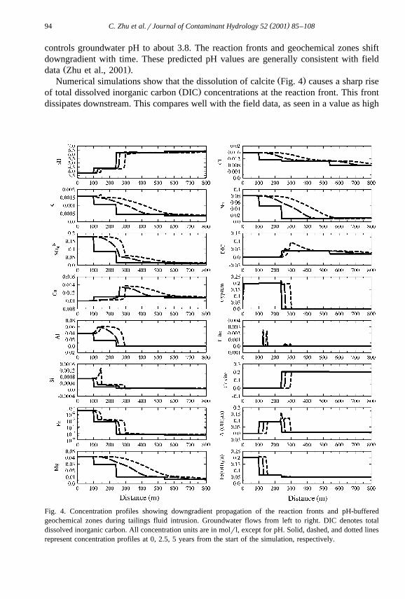
Ž .data Zhu et al., 2001 .Ž .Numerical simulations show that the dissolution of calcite Fig. 4 causes a sharp rise

Ž .of total dissolved inorganic carbon DIC concentrations at the reaction front. This frontdissipates downstream. This compares well with the field data, as seen in a value as high

Fig. 4. Concentration profiles showing downgradient propagation of the reaction fronts and pH-bufferedgeochemical zones during tailings fluid intrusion. Groundwater flows from left to right. DIC denotes totaldissolved inorganic carbon. All concentration units are in molrl, except for pH. Solid, dashed, and dotted linesrepresent concentration profiles at 0, 2.5, 5 years from the start of the simulation, respectively.


y Žas 0.029 molrl of HCO in the area immediate downstream from the plume Zhu et al.,3. Ž .2001 . Areas further downstream e.g., MW-14, Fig. 1 where the pH values are still

Ž .close to background level MW-36 in Fig. 1 have DIC as large as twice thebackground.

The predicted Al3q concentrations show a sharp drop at the calcite dissolution front,Ž . Ž .corresponding to the sharp rise of pH. Near the inlet, Al OH a is dissolved by the3

Ž . Ž . Ž .intruding tailings fluid Fig. 4 . Al OH a is dissolved at the upstream end and3Ž . Ž .accumulates at the downstream end of the Al OH a zone. The zone moves down-3

stream as the seepage continues.3q 3qŽ . 3qThe transport and reactions for Fe have a similar pattern to Al Fig. 4 . Fe is

y3 Ž . Ž .first reduced to the level of 10 molrl at the interface with Al OH a , and then3

reduced to 10y5 molrl level at the calcite dissolution front, in response to sharp pH rise.Downstream from the calcite dissolution front, Fe3q concentrations are nearly constant.

Ž .This prediction is consistent with field data e.g., MW-86 and MW-15 .Accompanied with calcite dissolution, gypsum is precipitated from groundwater and

Ž .sulfate concentrations are reduced sharply Fig. 4 . The gypsum zone advances down-stream at the same rate as that of the calcite dissolution front.

The numerical simulation predicts illite precipitation but no amorphous silica precipi-Ž . Ž .tation. Illite occurs at the Al OH a dissolution front as a single sharp peak, and a flat3

peak at the calcite dissolution front. This occurrence corresponds to higher pH and Al3q

Ž . Ž .concentrations at the Al OH a front. As illite is precipitated, aqueous silica concentra-3Ž .tions drop threefold Fig. 4 . Such a decrease is seen in the field data and laboratory

Ž .neutralization experiments Zhu et al., 2001 .The precipitation of illite only marginally affects Kq concentrations and has no

2q Ž .discernible effects on Mg concentrations Fig. 4 . In laboratory neutralization experi-2q q Žments of tailings fluids, the concentrations of Mg and K do not decrease see

.discussion in Zhu et al., 2001 . The decrease seen in field data can be either advective–dispersive transport or reactions with aquifer minerals or both. However, there areinsufficient field data to show whether the decrease is gradual or as sharp fronts. Field

q Ždata show an increase of Na from the calcite dissolution front and hence the higher2q .Ca concentration front , which may result from Ca–Na or Mg–Na exchange reac-

tions, which is common in sediment aquifers. However, Naq is not included in anyminerals in the model and essentially is modeled as a conservative tracer in this study.

4.2. Flushing by upgradient groundwater

Numerical simulation predicted several stages of geochemical evolution. First, theentrained acidic water in the pores continues to move downstream and the set ofreactions begun during the seepage period continues. Second, dissolution of gypsumoccurs because the incoming groundwater is undersaturated with it. Third, when allgypsum in the plume is expended, groundwater returns to background concentrationsafter a short period of perturbation.

Chemical reactions and advection–dispersion alternatively dominate the transport ofreactive constituents. For example, pH fronts first continue to advance downstream

Ž .because of the entrained acid in pore water Fig. 5 . The dissolution of gypsum near the



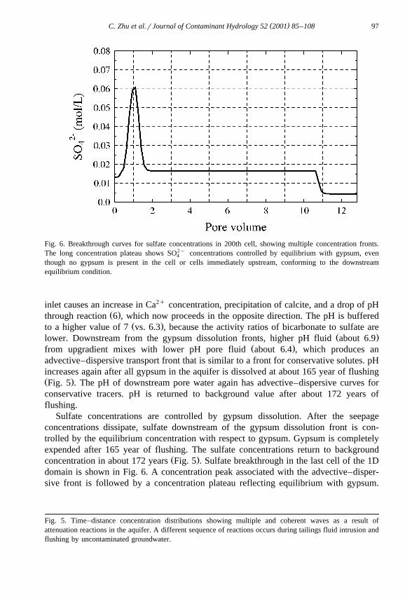
Fig. 6. Breakthrough curves for sulfate concentrations in 200th cell, showing multiple concentration fronts.The long concentration plateau shows SO2y concentrations controlled by equilibrium with gypsum, even4

though no gypsum is present in the cell or cells immediately upstream, conforming to the downstreamequilibrium condition.

inlet causes an increase in Ca2q concentration, precipitation of calcite, and a drop of pHŽ .through reaction 6 , which now proceeds in the opposite direction. The pH is buffered

Ž .to a higher value of 7 vs. 6.3 , because the activity ratios of bicarbonate to sulfate areŽ .lower. Downstream from the gypsum dissolution fronts, higher pH fluid about 6.9

Ž .from upgradient mixes with lower pH pore fluid about 6.4 , which produces anadvective–dispersive transport front that is similar to a front for conservative solutes. pHincreases again after all gypsum in the aquifer is dissolved at about 165 year of flushingŽ .Fig. 5 . The pH of downstream pore water again has advective–dispersive curves forconservative tracers. pH is returned to background value after about 172 years offlushing.

Sulfate concentrations are controlled by gypsum dissolution. After the seepageconcentrations dissipate, sulfate downstream of the gypsum dissolution front is con-trolled by the equilibrium concentration with respect to gypsum. Gypsum is completelyexpended after 165 year of flushing. The sulfate concentrations return to background

Ž .concentration in about 172 years Fig. 5 . Sulfate breakthrough in the last cell of the 1Ddomain is shown in Fig. 6. A concentration peak associated with the advective–disper-sive front is followed by a concentration plateau reflecting equilibrium with gypsum.

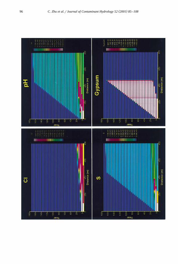
Fig. 5. Time–distance concentration distributions showing multiple and coherent waves as a result ofattenuation reactions in the aquifer. A different sequence of reactions occurs during tailings fluid intrusion andflushing by uncontaminated groundwater.


Here, no gypsum is present in the cell or cells immediately upstream so that theAdownstream equilibrium conditionB is observed. When gypsum was expended, SO2y

4

concentrations decreased to the background level.

4.3. Analysis of concentration waÕe propagation

The numerical modeling results are plotted in the time–space concentration distribu-Ž .tion diagrams Figs. 5 and 7 and analyzed using wave propagation theories. In these

diagrams, the flushing started at year 0 and the concentration distributions in the seepageperiod are shown in the negative time domain. Distinct concentration waves or fronts are

Ž .seen in these diagrams. Helfferich 1989 defined AwaveB as any variation of solute orsolid phase concentration and is synonymous with Afront.B For the convenience ofdiscussion, constant concentration levels for SO2y and gypsum have been traced and4

plotted in Fig. 7.

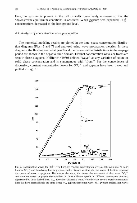
Fig. 7. Concentration waves for SO2y. The lines are constant concentration levels as labeled in molrl: solid4

lines for SO2y and thin dashed line for gypsum. In this distance vs. time plot, the slopes of the lines represent4

the speeds of wave propagation. The steeper the slope, the slower the movement of that wave. SO2y4

concentration waves propagate downgradient in three different speeds in different time–space domains,represented by thick dashed lines. W , advective–dispersive wave. Note there are several equal concentrationA

lines that have approximately the same slope; W , gypsum dissolution wave; W , gypsum precipitation wave.B C


The first type of wave for SO2y transport is the advection–dispersion wave, denoted4Ž .as W in Fig. 7. It has a propagation velocity equal to that of the pore fluid 50 mryear .A

The concentrations are smoothly diffused near the wavefront due to the dispersionŽincluded in the model. This type of wave is referred to as a AsalinityB wave Bryant et

.al., 1987; Schweich et al., 1993 . For solutes modeled as conservative tracers, namelyq y Ž y.Na and Cl , salinity waves are the only wave type for them see Fig. 5 for Cl .The second type of wave is the gypsum-dissolution wave, denoted as W in Fig. 7.B

Chemically, this wave represents the front of higher SO2y concentrations due to the4

dissolution of gypsum by uncontaminated upstream groundwater. The velocity of thiswave is less than that of the pore fluid. Measurement of the wavefronts from numericalsimulation indicates a speed of about 2.83 mryear. It is important to note that the Ca2q,SO2y, calcite precipitation, and pH decrease fronts that are involved in the gypsum4

dissolution process propagate at the same velocity, exhibiting a AcoherentB waveŽ .structure Helfferich and Klein, 1970; Walsh et al., 1984 . After all gypsum has been

dissolved at about 165 years flushing, SO2y propagates at the velocity of the advec-4

tion–dispersion wave as shown in Fig. 7.The third type of wave is the calcite dissolution and gypsum-precipitation wave,

denoted as W in Fig. 7. The calcite dissolution and gypsum precipitation waves areC

coherent with each other and coherent with the front of higher SO2y concentration4

because of the seepage of acidic tailings fluids. As shown in Fig. 7, the gypsum-precipi-Ž .tation wave propagates at a speed faster than the gypsum-dissolution wave W . As aB

result, the gypsum region widens as the flushing time increases until precipitation ends.Measured from the computed wavefronts, the gypsum-precipitation wave has a speed of

Ž 2q 2y 2y.16.36 mryear. Again, all components involved Ca , SO , pH, and CO propagate4 3

at the same speed and coherence is observed.The speeds of the above wave types are calculated analytically and compared to

numerical simulation results in Appendix A. It is shown in Appendix A that, whenconcentration plateaus exist at both sides of a concentration front, the wave speeds areindependent from hydrodynamic dispersion. Hence, the analytical solution for calculat-

Žing wave propagation speeds under advection and local equilibrium conditions Helf-.ferich and Klein, 1970 can be used to estimate, approximately, the wave speeds in the

Žpresence of hydrodynamic dispersion. Calculations using this analytical solution see.Appendix A show that the velocity of the calcite dissolution front is faster than the

gypsum dissolution front because Ca2q is present in solids at both sides of theŽ .dissolution wavefront calcite at the downstream and gypsum at the upstream and the

two solids have approximately equal mole concentrations. For the gypsum dissolutionŽ y6 .wave, only a trace amount of calcite precipitates at the upstream side ;10 molrl ,

Ž .but a large amount of gypsum 0.2 molrl exists at the downstream side of the wave.Wave speeds calculated from analytical solutions for gypsum dissolution and calcitedissolution are 2.83 and 17.16 mryear, which compare well with measured speeds fromnumerical modeling results of 2.82 and 16.36 mryear, respectively. Thus, numericalsimulations produce results that are consistent with analytical solutions. The simulatedresults where the calcite dissolution wave moves faster than the gypsum dissolutionwave are also consistent with chemical arguments. Precipitation of gypsum removesCa2q from the aqueous solution and creates lower chemical energy barriers, on the Ca2q


activity part, favoring more calcite dissolution. The quantity of calcite that can bedissolved depends on the advective–dispersive dissipation of the CO2y. It shows that in3

a reactive flow regime, the interplay of reactions and physical transport is significanteven when a local equilibrium condition is assumed.

4.4. SensitiÕity analysis and model limitations

Sensitivity analysis was conducted by varying hydraulic and geochemical parametersfor the seepage simulations. When all other parameters remain unchanged, higher flowvelocity would push the reaction fronts further downstream simply because more porevolumes of tailings fluid have reacted with the aquifer matrix.

The effects of dispersivity on reactive transport were evaluated by varying longitudi-nal dispersivity, a , from 10 to 0 and 80 m. With an a of 80 m, the reaction frontsL L

Ž . Ž .spread further downstream. The gypsum and Al OH a precipitation zones spread3

significantly broader toward downstream. As expected, conservative solutes spread outfurther with larger a values.L

Sensitivity analysis was also conducted by varying initial mineral concentrations inthe aquifer matrix and by including surface complexation reactions. The initial condi-tions have a significant impact on the distance of plume migration and duration ofnatural attenuation. As stated in the Introduction, the purpose of this study is not to findan answer for this site, but to explore the intricate interplay between physical transportand chemical reactions. Therefore, although the initial mineral concentrations aresignificant to practical concerns for the site, they do not alter the patterns of geochemicalevolution. Different mineral reactions in the geochemical model also change themodeling results. Inclusion of surface reactions does not significantly change thereactive transport in the seepage period, but significantly increases acidity in the plume.These reaction patterns are quite complex and are the subject of ongoing research.

Despite their complexity, the present model results are far from a complete answer tothe problem in this area, but they are a step in the right direction. One of the advantagesof numerical modeling is that important factors, which are poorly known or unknown,can be revealed. We also realize that it is prudent to build our knowledge in a phasedapproach from simple to more complex models. Hence, this study only dealt with themigration of major groundwater constituents. The model limitations are obvious:

Ž .1 A uniform and constant Darcy velocity was assumed whereas drainage of tailingsfluid in the aquifer changes hydraulic gradients. The negligence of mixing of water fromboth sides of the alluvium channel along the 1D domain probably resulted in anunderestimation of the dilution effect.

Ž . Ž .2 The local equilibrium assumption was used Knapp, 1989 . However, reactionsthat are known to be controlled by kinetics such as feldspar dissolution and quartzprecipitation were not included in the model. The use of illite as an equilibrium phase

Ž .and the sink for SiO aq is not well supported by field evidence, although illite2

precipitation has negligible effects in the overall modeling results.Ž .3 The porosity of the porous media is constant during flow. Thus, the reactive solids

only occupy small fractions of the bulk media. Dissolution and precipitation of 0.2


molrl gypsum would change about 1.5% porosity. The simulations assumed that it hasnegligible effects on the transport.

Ž .4 The precipitates are stationary, e.g., precipitates are not transported with the flowas colloids. It is possible that amorphous Fe and Al hydroxides form colloidal materialsin the aquifer.

Ž .5 TDS contents in the tailings fluids and background water are significantlydifferent. Thus, the density of fluids may have significant effect on solute transport.

Ž .6 The actual mineral assemblage, both primary and secondary, their relativeabundances, and spatial distributions are very important to the modeling results.However, no detailed mineralogical data are available.

Ž .7 More chemical reactions like cation exchange and surface reactions may beoperative in the field but neglected in the model.

5. Summary and conclusions

The migration of major groundwater constituents under a reclamation scenario of auranium mill tailings impoundment was simulated using the reactive mass transportmodel PHREEQC. A detailed geochemical model was included in the transport simulation.Two types of conditions were simulated: seepage of acidic tailings fluid into a shallowsandy aquifer and flushing by upgradient uncontaminated groundwater after the sourceof contamination is terminated. Each of the conditions produced a set of chemicalreaction and transport patterns that are typical for acid mine drainage contamination ofan aquifer or a remediationrnatural attenuation scheme. Therefore, the results ofsimulation have general implications for acid mine drainage problems.

The simulations show that:Ž . 2y1 For acidic tailings fluid seepage condition, the numerical model predicted SO ,4

Ca2q, Fe3q, Al3q, CO2y, and Hq distributions in distinct geochemical zones, controlled3Ž . Ž . Ž . Ž .by pH buffer reactions with calcite, Al OH a , and Fe OH a , respectively. Simu-3 3

lated pattern, sequence, and concentration levels are comparable to field data althoughthe forward model cannot be compared to the spatial and temporal information in thefield. Most mass transfer reactions occur at the interfaces of different geochemical

Ž .zones. Hence, the successive pH buffer reaction model of Zhu et al. 2001 , inferredfrom field data and batch-scale static geochemical modeling, appears to interpretsuccessfully the field data when transport processes are included in simulations. Thistransport and reaction pattern should be general for all acid mine drainage systemswhere calcite is present.

Ž .2 Numerical modeling predicts several stages of geochemical evolution during theflushing of contaminated sediments by uncontaminated upgradient groundwater. Gyp-sum dissolution drives the pH, SO2y, and Ca2q concentration distributions and this was4

followed by advective–dispersive transport. The duration of natural attenuation dependson the initial conditions in the model. This dependence remains to be investigated.Model predictions can also be assessed by examining monitoring data at this site in thefuture.


Ž .3 In different time–space domains, the transport of reactive constituents is domi-nated alternatively by chemical reactions or physical transport processes, which pro-duces multiple concentration waves that have different speeds. In the case of SO2y, the4

waves are controlled by advection–dispersion, gypsum precipitation, gypsum dissolu-tion, and then advective–dispersive transport, in a sequence. ACoherentB waves fordifferent constituents were also produced. Simulated wave speeds compare well to thosecalculated from an analytical solution.

Acknowledgements

We are indebted to Gary Chase and Ernie Scott of Awadarko Petroleum Corporationfor their permission to use the site data to conduct research and publication of the resultsand to David Parkhurst and Tony Appelo for discussions on the use of PHREEQC 2.0. Wethank Greg Anderson, Martin Appold, Karen Salvage, Frank Schwartz, and MotomuIbaraki for review of the manuscript. Although the research described in this article hasbeen funded wholly or in part by US Environmental Protection Agency, it has not beensubject to the Agency’s review and therefore does not necessarily reflect the views ofthe Agency, and no official endorsement should be inferred. Permission by UnionPacific Resources for publishing the modeling results does not necessarily reflect theiragreement with the approaches or parameters used in the model or model predictions.Assistance from Dana McClish in various aspects of this work is greatly appreciated.

Appendix A. A note on the wave propagation speed in the presence of dispersion

In this appendix, we consider the propagation speed of the precipitation and dissolu-tion waves in the presence of dispersivity and give an approximate solution forestimating the wave speed.

When dispersion is not present, the precipitation and dissolution wavefronts are sharpŽand their propagation speeds have been derived and given in the literature e.g.,

.Helfferich and Klein, 1970 . The speed of the wave is related to the jump conditionsacross the wavefront. When dispersion is present, concentration changes are moregradual near the wavefronts as seen in our calculations. We will show, however, that thewave speed can still be related to the values of concentrations across the wavefrontunder the conditions given below.

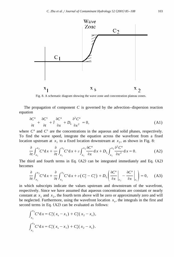
Our numerical calculations indicate that, in many cases, concentration plateau zonesare still formed in the presence of dispersion, as illustrated in Fig. 8. Our discussionswill be based on the assumption that concentrations are constant, or nearly constant,upstream and downstream of the wave zone. In addition, we also assume that the porevelocity Õ and dispersivity D are constant, as in our numerical calculations. ToL

facilitate our discussions, we will define the location of a wavefront x such that thes

shaded areas in Fig. 8 are the same.


Fig. 8. A schematic diagram showing the wave zone and concentration plateau zones.

The propagation of component C is governed by the advection–dispersion reactionequation

ECa EC s ECa E2 Ca

q qÕ qD s0, A1Ž .L 2Et Et Ex Ex

where Ca and C s are the concentrations in the aqueous and solid phases, respectively.To find the wave speed, integrate the equation across the wavefront from a fixedlocation upstream at x to a fixed location downstream at x , as shown in Fig. 8:1 2

x x x a x 2 aE E EC E C2 2 2 2a sC d xq C d xqÕ d xqD d xs0. A2Ž .H H H HL 2Et Et Ex Exx x x x1 1 1 1

Ž . Ž .The third and fourth terms in Eq. A2 can be integrated immediately and Eq. A2becomes

a ax xE E EC EC2 2a s a aC d xq C d xqÕ C yC qD y s0, A3Ž .Ž .H H 2 1 L ž /Et Et Ex Exx x x x1 1 2 1

in which subscripts indicate the values upstream and downstream of the wavefront,respectively. Since we have assumed that aqueous concentrations are constant or nearlyconstant at x and x , the fourth term above will be zero or approximately zero and will1 2

be neglected. Furthermore, using the wavefront location x , the integrals in the first andsŽ .second terms in Eq. A2 can be evaluated as follows:

x2 a a aC d xsC x yx qC x yx ,Ž . Ž .H 1 s 1 2 2 sx1

x2 s s sC d xsC x yx qC x yx .Ž . Ž .H 1 s 1 2 2 sx1


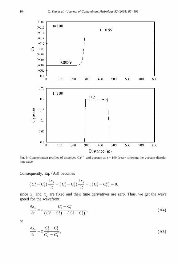
2q Ž .Fig. 9. Concentration profiles of dissolved Ca and gypsum at ts100 year , showing the gypsum-dissolu-tion wave.

Ž .Consequently, Eq. A3 becomes

Ex Exs sa a s s a aC yC q C yC qÕ C yC s0,Ž . Ž . Ž .1 2 1 2 2 1Et Et

since x and x are fixed and their time derivatives are zero. Thus, we get the wave1 2

speed for the wavefront

Ex CayCas 2 1sÕ , A4Ž .a a s sEt C yC q C yCŽ . Ž .2 1 2 1

or

Ex CayCas 2 1sÕ , A5Ž .T TEt C yC2 1


where C T is the total concentration of the component in both the aqueous and solidphases. We note that the above formula is the same as those derived for waves when

Ž .dispersion is not present Helfferich and Klein, 1970 . It shows that this formula is stillapplicable as long as concentration plateau zones are formed adjacent to a wavefront.When concentration plateau zones are not formed, as we have seen in our numerical

Ž .simulations for some components, Eq. A5 is not accurate.

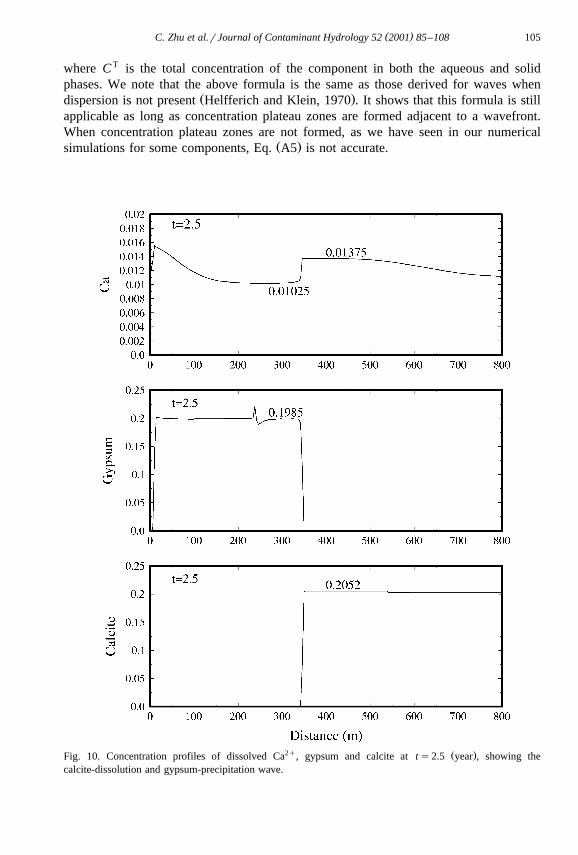
2q Ž .Fig. 10. Concentration profiles of dissolved Ca , gypsum and calcite at ts2.5 year , showing thecalcite-dissolution and gypsum-precipitation wave.


Ž .To demonstrate the validity of Eq. A5 , two examples from our numerical resultswill be shown below.

Ž . 2qFirst, consider the gypsum dissolution wave W in Fig. 7 , using Ca concentra-B

tion for calculation. Profiles of relevant distributions are plotted in Fig. 9 with indicatedŽ .plateau values. Here, we have Õs50 mryear and

Cas0.0039, C Ts0.00391 1

Cas0.0159, C Ts0.0039q0.2s0.20392 2

0.0159y0.0039wave speeds50 s2.83 mryearŽ .

0.2159y0.0039

The measured wave speed from numerical simulation, shown in Fig. 7, is 2.82 mryear.A very good agreement is seen.

ŽSecond, consider the calcite-dissolution and gypsum-precipitation wave W in Fig.C. 2q7 . Profiles of the concentrations of Ca , gypsum and calcite are shown in Fig. 10.

Here, we have

Cas0.01025, C Ts0.01025q0.1985s0.20851 1

Cas0.01375, C Ts0.01375q0.2052s0.218952 2

0.01375y0.01025wave speeds50 s17.16 mryearŽ .

0.21895y0.2085

The measured wave speed from numerical simulations is 16.36 mryear, a closeagreement.

Finally, we note that precipitation and dissolution of solid phases can result inchanges of pore velocities Õ and dispersivity D . The condition of constant velocity andL

dispersivity may be least satisfied in the vicinity of a wavefront, but necessary for theŽ .derivation of Eq. A5 . Because this condition is the same for numerical simulations, the

agreement between numerical and analytical results does not validate the applicability ofŽ .Eq. A5 .

References

Appelo, C.A.J., Postma, D., 1994. Geochemistry, Groundwater, and Pollution. Balema, Rotterdam.Bear, J., 1972. Dynamics of Fluids in Porous Media. Dover Publications, New York, NY.Bethke, C.M., Brady, P.V., 2000. How the Kd approach undermines ground water cleanup. Ground Water 38

Ž .3 , 435–443.Bryant, S.L., Schechter, R.S., Lake, L.W., 1987. Mineral sequences in precipitationrdissolution waves.

Ž .AIChE Journal 33 8 , 1271–1287.Cederberg, G.A., Leckie, J.O., Street, R.L., 1985. A groundwater mass transport and equilibrium chemistry

model for multicomponent systems. Water Resource Research 21, 1095–1104.Glynn, P., Brown, J., 1996. Reactive transport modeling of acid metal-contaminated groundwater at a site with


Ž .sparse spatial information. In: Lichtner, P.C., Steefel, C.I., Oelkers, E.H. Eds. , Reactive Transport inPorous Media. Review in Mineralogy, Mineralogical Society of America, Washington, DC.

Ž .Helfferich, F.G., 1989. The theory of precipitationrdissolution waves. AIChE Journal 35 1 , 75–87.Helfferich, F.G., Klein, G., 1970. Multicomponent Chromatography. Marcel Dekker, New York, NY.

Ž .King, T.V.V. Ed. , 1995.Environmental considerations of active and abandoned mine lands. United StatesGeological Survey Bulletin, 2220.

Knapp, R.A., 1989. Spatial and temporal scales of local equilibrium in dynamic fluid–rock systems.Geochimica et Cosmochimica Acta 53, 1955–1964.

Lichtner, P., 1985. Continuum model for simultaneous chemical reactions and mass transport in hydrothermalsystems. Geochimica et Cosmochimica Acta 49, 779–800.

Mangold, D.C., Tsang, C.F., 1991. A summary of subsurface hydrological and hydrochemical models.Reviews of Geophysics 29, 51–79.

Nordstrom, D.K., Busenberg, E., Jones, B.F., Langmuir, D., May, H.M., Parkhurst, D.L., Plummer, L.N.,1990. Revised chemical equilibrium data for major water–mineral reactions and their limitations. In:

Ž .Bassett, R., Melchoir, D. Eds. , Chemical Modeling in Aqueous Systems II. Am. Chem. Soc. Symp. Ser.416, 398–413.

Parkhurst, D.L., 1995. User’s guide to PHREEQC–a computer program for speciation, reaction-path, advective-transport, and inverse geochemical modeling. U.S. Geological Survey, Water-Resource InvestigationReport, pp. 95–4227.

Ž .Parkhurst, D.L., Appello, A.A.J., 1999. User’s guide to PHREEQC version 2 –a computer program forspeciation, batch-reaction, one dimensional transport, and inverse geochemical modeling. U.S. GeologicalSurvey, Water-Resource Investigation Report, pp. 99–4259.

Raffensperger, J.P., Garven, G., 1995. The formation of unconforming-type uranium ore deposit: 2. Coupledhydrochemical modeling. American Journal of Science 295, 581–636.

Reardon, E.J., 1981. Kd’s—Can they be used to describe reversible ion sorption reactions in contaminantŽ .migration? Ground Water 19 3 , 279–286.

Sharp, W.N., Gibbons, A.B., 1964. Geology and uranium deposits of the southern part of the Powder Riverbasin, Wyoming. USGS Bulletin, 1147-D.

Schwartz, F.W., Domenico, P.A., 1973. Simulation of hydrochemical patterns in regional groundwater flow.Water Resources Research 9, 1293–1297.

Schweich, D., Sardin, M., Jauzein, M., 1993. Properties of concentration waves in presence of nonlinearsorption, precipitationrdissolution, and homogenous reactions: 1. Fundamentals. Water Resource Research24, 723–733.

Steefel, C., Lasaga, A., 1994. A coupled model for transport of multiple chemical species and kineticprecipitationrdissolution reactions with applications to reactive flow in single phase hydrothermal systems.American Journal of Science 294, 529–592.

Steefel, C., MacQuarrie, K.T.B., 1996. Approaches to modeling of reactive transport in porous media. In:Ž .Lichtner, P.C., Steefel, C.I., Oelkers, E.H. Eds. , Reactive Transport in Porous Media. Review in

Mineralogy, Mineralogical Society of America, Washington, DC, pp. 83–130.Stumm, W., Morgan, J., 1981. Aquatic Chemistry—Chemical Equilibria and Rates in Natural Waters. Wiley,

New York, NY.Walsh, M.P., 1983. Geochemical Flow Modeling. PhD dissertation, University of Texas, Austin, TX.Walsh, M.P., Bryant, S.L., Lake, L.W., Schechter, R.S., 1984. Precipitation and dissolution of solids attending

Ž .flow through porous media. AIChE Journal 30 2 , 317–328.Walter, A.L., Blowes, D.W., Frind, E.O., Molson, J.W., Ptacek, C.J., 1994a. Modeling of multicomponent

reactive transport in groundwater: 1. Model development and evaluation. Water Resources Research 30,3137–3148.

Walter, A.L., Blowes, D.W., Frind, E.O., Molson, J.W., Ptacek, C.J., 1994b. Modeling of multicomponentreactive transport in groundwater. 2. Metal mobility in aquifers impacted by acidic mine tailings discharge.Water Resources Research 30, 3149–3158.

Yeh, G.T., Tripathi, V.S., 1989. A critical evaluation of recent development of hydrogeochemical transportŽ .models of reactive multi-components. Water Resource Research 25 1 , 93–108.

Yeh, G.T., Tripathi, V.S., 1991. A model for simulating transport of reactive multispecies components: modelŽ .development and demonstration. Water Resource Research 27 12 , 3075–3094.


Zhu, C., Waddell, R.K., Yeh, G.T., 1996. TRANSRXN—a coupled geochemical model and hydrologicalmodel with coprecipitation for simulation of reactive transport in groundwater systems. Submitted to USEPA.

Zhu, C., Anderson, G.M., Burden, D.S., 2001. Geochemical modeling of natural attenuation reactions in aŽ .contaminated shallow aquifer at a uranium mill tailings site, western USA. Ground Water in press .

Multicomponent reactive transport modeling of uranium bioremediation field experiments

Documents