Multiclass Recognition and Part Localization with Humans in the Loop Catherine Wah † Steve Branson † † Department of Computer Science and Engineering University of California, San Diego {cwah,sbranson,sjb}@cs.ucsd.edu Pietro Perona ‡ Serge Belongie † ‡ Department of Electrical Engineering California Institute of Technology [email protected] Abstract We propose a visual recognition system that is designed for fine-grained visual categorization. The system is com- posed of a machine and a human user. The user, who is un- able to carry out the recognition task by himself, is interac- tively asked to provide two heterogeneous forms of informa- tion: clicking on object parts and answering binary ques- tions. The machine intelligently selects the most informative question to pose to the user in order to identify the object’s class as quickly as possible. By leveraging computer vision and analyzing the user responses, the overall amount of hu- man effort required, measured in seconds, is minimized. We demonstrate promising results on a challenging dataset of uncropped images, achieving a significant average reduc- tion in human effort over previous methods. 1. Introduction Vision researchers have become increasingly interested in recognition of parts [2, 8, 21], attributes [6, 11, 12], and fine-grained categories (e.g. specific species of birds, flow- ers, or insects) [1, 3, 14, 15]. Beyond traditionally studied basic-level categories, these interests have led to progress in transfer learning and learning from fewer training ex- amples [7, 8, 10, 15, 21], larger scale computer vision al- gorithms that share processing between tasks [15, 16], and new methodologies for data collection and annotation [2, 4]. Parts, attributes, and fine-grained categories push the limits of human expertise and are often inherently ambigu- ous concepts. For example, perception of the precise lo- cation of a particular part (such as a bird’s beak) can vary from person to person, as does perception of whether or not an object is shiny. Fine-grained categories are usually recognized only by experts (e.g. the average person cannot recognize a Myrtle Warbler), while one can recognize im- mediately basic categories like cows and bottles. We propose a key conceptual simplification: that humans and computers alike should be treated as valuable but ulti- mately imperfect sources of information. Humans are able Q1: Click on the head (3.656 s) IMAGE CLASS: Sooty Albatross Ground Truth Part Locations Sooty Albatross? yes Bohemian Waxwing? no FŽƌƐƚĞƌƐ TĞƌŶ no Q2: Click on the body (3.033 s) Body Head Beak Wing Tail Breast Predicted Part Locations Q3: Is the bill black? yes (4.274 s) Black-footed Albatross? no Figure 1. Our system can query the user for input in the form of binary attribute questions or part clicks. In this illustrative exam- ple, the system provides an estimate for the pose and part locations of the object at each stage. Given a user-clicked location of a part, the probability distributions for locations of the other parts in each pose will adjust accordingly. The rightmost column depicts the maximum likelihood estimate for part locations. to detect and broadly categorize objects, even when they do not recognize them, as well as carry out simple mea- surements such as telling color and shape; human errors arise primarily because (1) people have limited experiences and memory, and (2) people have subjective and percep- tual differences. In contrast, computers can run identical pieces of software and aggregate large databases of infor- mation. They excel at memory-based problems like recog- nizing movie posters but struggle at detecting and recog- nizing objects that are non-textured, immersed in clutter, or highly shape-deformable. In order to achieve a unified treatment of humans and computers, we introduce models and algorithms that ac- count for errors and inaccuracies of vision algorithms (part localization, attribute detection, and object classification) and ambiguities in multiple forms of human feedback (per- ception of part locations, attribute values, and class labels). The strengths and weaknesses of humans and computers for

Welcome message from author
This document is posted to help you gain knowledge. Please leave a comment to let me know what you think about it! Share it to your friends and learn new things together.
Transcript
Multiclass Recognition and Part Localization with Humans in the Loop
Catherine Wah† Steve Branson†
†Department of Computer Science and Engineering
University of California, San Diego
{cwah,sbranson,sjb}@cs.ucsd.edu
Pietro Perona‡ Serge Belongie†
‡Department of Electrical Engineering
California Institute of Technology
Abstract
We propose a visual recognition system that is designed
for fine-grained visual categorization. The system is com-
posed of a machine and a human user. The user, who is un-
able to carry out the recognition task by himself, is interac-
tively asked to provide two heterogeneous forms of informa-
tion: clicking on object parts and answering binary ques-
tions. The machine intelligently selects the most informative
question to pose to the user in order to identify the object’s
class as quickly as possible. By leveraging computer vision
and analyzing the user responses, the overall amount of hu-
man effort required, measured in seconds, is minimized. We
demonstrate promising results on a challenging dataset of
uncropped images, achieving a significant average reduc-
tion in human effort over previous methods.
1. Introduction
Vision researchers have become increasingly interested
in recognition of parts [2, 8, 21], attributes [6, 11, 12], and
fine-grained categories (e.g. specific species of birds, flow-
ers, or insects) [1, 3, 14, 15]. Beyond traditionally studied
basic-level categories, these interests have led to progress
in transfer learning and learning from fewer training ex-
amples [7, 8, 10, 15, 21], larger scale computer vision al-
gorithms that share processing between tasks [15, 16], and
new methodologies for data collection and annotation [2, 4].
Parts, attributes, and fine-grained categories push the
limits of human expertise and are often inherently ambigu-
ous concepts. For example, perception of the precise lo-
cation of a particular part (such as a bird’s beak) can vary
from person to person, as does perception of whether or
not an object is shiny. Fine-grained categories are usually
recognized only by experts (e.g. the average person cannot
recognize a Myrtle Warbler), while one can recognize im-
mediately basic categories like cows and bottles.
We propose a key conceptual simplification: that humans
and computers alike should be treated as valuable but ulti-
mately imperfect sources of information. Humans are able
Q1: Click on the head
(3.656 s)
IMAGE CLASS: Sooty Albatross
Ground Truth Part Locations
Sooty Albatross? yes
Bohemian Waxwing? no
FラヴゲデWヴげゲ TWヴミい no
Q2: Click on the body
(3.033 s)
Body
Head
Beak
Wing
Tail Breast
Predicted Part Locations
Q3: Is the bill black?
yes (4.274 s)
Black-footed Albatross? no
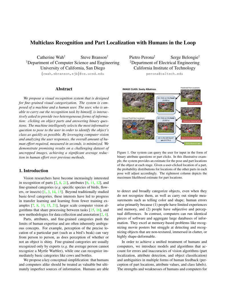
Figure 1. Our system can query the user for input in the form of
binary attribute questions or part clicks. In this illustrative exam-
ple, the system provides an estimate for the pose and part locations
of the object at each stage. Given a user-clicked location of a part,
the probability distributions for locations of the other parts in each
pose will adjust accordingly. The rightmost column depicts the
maximum likelihood estimate for part locations.
to detect and broadly categorize objects, even when they
do not recognize them, as well as carry out simple mea-
surements such as telling color and shape; human errors
arise primarily because (1) people have limited experiences
and memory, and (2) people have subjective and percep-
tual differences. In contrast, computers can run identical
pieces of software and aggregate large databases of infor-
mation. They excel at memory-based problems like recog-
nizing movie posters but struggle at detecting and recog-
nizing objects that are non-textured, immersed in clutter, or
highly shape-deformable.
In order to achieve a unified treatment of humans and
computers, we introduce models and algorithms that ac-
count for errors and inaccuracies of vision algorithms (part
localization, attribute detection, and object classification)
and ambiguities in multiple forms of human feedback (per-
ception of part locations, attribute values, and class labels).
The strengths and weaknesses of humans and computers for

facing_right facing_left body_horizontal_right head_turned_left body_horizontal_left
head_turned_right fly_swim_towards_right body_vertical_facing_left fly_swim_towards_left body_vertical_facing_right
(a) Pose clusters
}~),~,~{(~
ppppvyx
User Click Location
}),,{(pppp
vyxGround Truth Location
),(pp
x Features
(b) User interface for part locations input
Figure 2. 2(a) Images in our dataset are clustered by k-means on the spatial offsets of part locations from parent part locations. Semantic
labels of clusters were manually assigned by visual inspection. Left/right orientation is in reference to the image. 2(b) The user clicks on
his/her perceived location of the breast (xp, yp), which is shown as a red X and is assumed to be near the ground truth location (xp, yp).The user also can click a checkbox indicating part visibility vp. Features ψp(x, θp) can be extracted from a box around θp.
these modalities are combined using a single principled ob-
jective function: minimizing the expected amount of time
to complete a given classification task.
Consider for example different types of human annota-
tion tasks in the domain of bird species recognition. For the
task “Click on the beak,” the location a human user clicks
is a noisy representation of the ground truth location of the
beak. It may not in isolation solve any single recognition
task; however, it provides information that is useful to a
machine vision algorithm for localizing other parts of the
bird, measuring attributes (e.g. cone-shaped), recognizing
actions (e.g. eating or flying), and ultimately recognizing
the bird species. The answer to the question “Is the belly
striped?” similarly provides information towards recogniz-
ing a variety of bird species. Each type of annotation takes
a different amount of human time to complete and provides
varying amounts of information.
Our models and algorithms combine all such sources of
information into a single principled framework. We have
implemented a practical real-time system1 for bird species
identification on a dataset of over 200 categories. Recog-
nition and pose registration can be achieved automatically
using computer vision; the system can also incorporate hu-
man feedback when computer vision is unsuccessful by in-
telligently posing questions to human users (see Figure 1).
The contributions of this paper are: (1) We introduce
models and algorithms for object detection, part localiza-
tion, and category recognition that scale efficiently to large
numbers of categories. Our algorithms can localize and
classify objects on a 200-class dataset in a fraction of a sec-
ond, using part and attribute detectors that are shared among
classes. (2) We introduce a formal model for evaluating the
usefulness of different types of human input that takes into
account varying levels of human error, time spent, and in-
formativeness in a multiclass or multitask setting. We intro-
duce fast algorithms that are able to predict the informative-
ness of 312 binary questions and 13 part click questions in a
1See http://visipedia.org/ for a demo of our system.
fraction of a second. All such computer vision algorithms,
forms of user input, and question selection techniques are
combined into an integrated framework. (3) We present a
thorough experimental comparison of a number of methods
for optimizing human input.
The structure of the paper is as follows: In Section 2, we
review related work. We define the problem and describe
the algorithm in Sections 3 and 4. In Section 5 we discuss
implementation details, in Section 6 we present empirical
results, and finally in Section 7 we discuss future work.
2. Related Work
Our work extends prior work by Branson et al. [3],
who introduced a system combining human interaction with
computer vision that was applied to bird species classifi-
cation. They used an information-theoretic framework to
intelligently select attribute questions such as “Is the belly
spotted?”, “Is the wing white?”, etc. to identify the true bird
species as quickly as possible. Our work has 3 main dif-
ferences: (1) While [3] used non-localized computer vision
methods based on bag-of-words features extracted from the
entire image, we use localized part and attribute detectors.
Thus [3] relied on experiments with test images cropped by
ground truth bounding boxes; in contrast, our experiments
are performed on uncropped images in unconstrained en-
vironments. (2) Whereas [3] incorporated only one type
of user input – binary questions pertaining to attributes –
we allow heterogeneous forms of user input including user-
clicked part locations. Users can click on any pixel location
in an image, introducing significant algorithmic and com-
putational challenges as we must reason over hundreds of
thousands of possible click point and part locations. (3)
Whereas [3] measured human effort in terms of the total
number of questions asked, we introduce an extended ques-
tion selection criterion that factors in the expected amount
of human time needed to answer each type of question.
A number of papers have recently addressed fine-grained
categorization [1, 3, 13, 14, 15, 22]. One important differ-

ence between this paper and prior work is that we use local-
ized computer vision algorithms based on part and attribute
detectors (in contrast, [3, 13, 14, 15] rely on bag-of-words
methods). The differences between fine-grained categories
are subtle, such that it is likely that lossy representations
such as bag-of-words are insufficient. Bird field guides [19]
suggest that humans use strongly localized methods based
on parts and attributes to perform bird species recognition,
justifying our approach. Also, we introduce an extended
version of the CUB-200 dataset [18] that consists of 200bird species and nearly 12, 000 images, each of which is la-
beled with part locations and attribute annotations (example
images are shown in Figure 2(a)). Additional discussion of
related work covered in [3] is not revisited here.
Our integrated approach builds on two areas in com-
puter vision: part-based models and attribute-based learn-
ing, which have both been explored in depth in other
works. Specifically, we use a part representation simi-
lar to a Felzenszwalb-style deformable part model [8, 9]
(sliding window HOG-based part detectors fused with tree-
structured spatial dependencies). Whereas most attribute-
based methods [6, 12] use non-localized classifiers, [5,
20] incorporate object or part-level localization with at-
tribute detectors. Our methods differ from earlier work
on parts and attributes by (1) the specific combination of
a Felzenszwalb-style deformable part model with localized
attribute detectors, (2) the additional ability to combine part
and attribute models with different types of user input, and
(3) the deployment of such methods on a dataset of larger
scale, localizing 200 object classes, 13 parts, 11 aspects,
and 312 binary attributes in a fraction of a second.
3. Framework for Visual Recognition
In this section, we introduce a principled framework for
integrating part-based detectors, multi-class categorization
algorithms, and different types of human feedback into a
common probabilistic model. We also introduce efficient
algorithms for inferring and updating object class and lo-
calization predictions as additional user input is obtained.
We begin by formally defining the problem.
3.1. Problem Definition and Notation
Given an image x, our goal is to predict an object class
from a set of C possible classes (e.g. Myrtle Warbler, Blue
Jay, Indigo Bunting) within a common basic-level category
(e.g. Birds). We assume that the C classes fall within a
reasonably homogeneous basic-level category such as birds
that can be represented using a common vocabulary of P
parts (e.g. head, belly, wing), and A attributes (e.g. cone-
shaped beak, white belly, striped breast). We use a class-
attribute model based on the direct-attribute model of Lam-
pert et al. [12], where each class c ∈ 1...C is represented us-
ing a unique, deterministic vector of attribute memberships
ac = [ac1...a
cA], a
ci ∈ 0, 1. We extend this model to include
part localized attributes, such that each attribute a ∈ 1...Acan optionally be associated with a part part(a) ∈ 1...P(e.g. the attributes white belly and striped belly are both as-
sociated with the part belly). In this case, we express the set
of all ground truth part locations for a particular object as
Θ = {θ1...θP }, where the location θp of a particular part p
is represented as an xp, yp image location, a scale sp, and an
aspect vp (e.g. side view left, side view right, frontal view,
not visible, etc.):
θp = {xp, yp, sp, vp}. (1)
Note that the special aspect not visible is used to handle
parts that are occluded or self-occluded.
We can optionally combine our computer vision algo-
rithms with human input, by intelligently querying user in-
put at runtime. A human is capable of providing two types
of user input which indirectly provide information relevant
for predicting the object’s class: mouse click locations θpand attribute question answers ai. The random variable
θp represents a user’s input of the part location θp, which
may differ from user to user due to both clicking inaccura-
cies and subjective differences in human perception (Figure
2(b)). Similarly, ai is a random variable defining a user’s
perception of the attribute value ai.
We assume a pool of A + P possible questions that can
be posed to a human user Q = {q1...qA, qA+1...qA+P },
where the first A questions query ai and the remaining P
questions query θp. Let Aj be the set of possible answers to
question qj . At each time step t, our algorithm considers the
visual content of the image and the current history of ques-
tion responses to estimate a distribution over the location of
each part, predict the probability of each class, and intelli-
gently select the next question to ask qj(t). A user provides
the response uj(t) to a question qj(t), which is the value of
θp or ai for part location or attribute questions, respectively.
The set of all user responses up to timestep t is denoted by
the symbol U t = {uj(1)...uj(t)}. We assume that the user
is consistent in answering questions and therefore the same
question is never asked twice.
3.1.1 Probabilistic Model
Our probabilistic model incorporating both computer vision
and human user responses is summarized in Figure 3(b).
Our goal is to estimate the probability of each class given
an arbitrary collection of user responses U t and observed
image pixels x:
p(c|U t, x) =p(ac, U t|x)
∑
c p(ac, U t|x)
, (2)
which follows from the assumption of unique, class-
deterministic attribute memberships ac [12]. We can in-

(a) Part Model (b) Part-Attribute Model
Figure 3. Probabilistic Model. 3(a): The spatial relationship be-
tween parts has a hierarchical independence structure. 3(b): Our
model employs attribute estimators, where part variables θp are
connected using the hierarchical model shown in 3(a).
corporate localization information Θ into the model by in-
tegrating over all possible assignments to part locations
p(ac, U t|x) =
∫
Θ
p(ac, U t,Θ|x)dΘ. (3)
We can write out each component of Eq 3 as
p(ac, U t,Θ|x) = p(ac|Θ, x)p(Θ|x)p(U t|ac,Θ, x) (4)
where p(ac|Θ, x) is the response of a set of attribute de-
tectors evaluated at locations Θ, p(Θ|x) is the response of
a part-based detector, and p(U t|ac,Θ, x) models the way
users answer questions. We describe each of these proba-
bility distributions in Sections 3.2.1, 3.2.2, and 3.3 respec-
tively and describe inference procedures for evaluating Eq 3
efficiently in Section 3.4.
3.2. Computer Vision Model
As described in Eq 4, we require two basic types of com-
puter vision algorithms: one that estimates attribute proba-
bilities p(ac|Θ, x) on a particular set of predicted part loca-
tions Θ, and another that estimates part location probabili-
ties p(Θ|x).
3.2.1 Attribute Detection
Using the independence assumptions depicted in Figure
3(b), we can write the probability
p(ac|Θ, x) =∏
aci∈a
c
p(aci |θpart(ai), x). (5)
Given a training set with labeled part locations θpart(ai), one
can use standard computer vision techniques to learn an es-
timator for each p(ai|θpart(ai), x). In practice, we train a
separate binary classifier for each attribute, extracting lo-
calized features from the ground truth location θpart(ai).
As in [12], we convert attribute classification scores zi =fa(x; part(ai)) to probabilities by fitting a sigmoid func-
tion σ(γazi) and learning the sigmoid parameter γa using
cross-validation. When vpart(ai) = not visible, we assume
the attribute detection score is zero.
3.2.2 Part Detection
We use a pictorial structure to model part relationships (see
Figure 3(a)), where parts are arranged in a tree-structured
graph T = (V,E). Our part model is a variant of the model
used by Felzenszwalb et al. [8], which models the detection
score g(x; Θ) as a sum over unary and pairwise potentials
log(p(Θ|x)) ∝ g(x; Θ) with
g(x; Θ) =
P∑
p=1
ψ(x; θp) +∑
(p,q)∈E
λ(θp, θq) (6)
where each unary potential ψ(x; θp) is the response of a
sliding window detector, and each pairwise score λ(θp, θq)encodes a likelihood over the relative displacement between
adjacent parts. We use the same learning algorithms and
parametrization of each term in Eq 6 as in [23]. Here,
parts and aspects are semantically defined, multiple aspects
are handled using mixture models, and weight parameters
for appearance and spatial terms are learned jointly using a
structured SVM [17]. After training, we convert detection
scores to probabilities p(Θ|x) ∝ exp (γg(x; Θ)), where γ
is a scaling parameter that is learned using cross-validation.
3.3. User Model
Readers interested in a computer-vision-only system
with no human-in-the-loop can skip to Section 3.4. We as-
sume that the probability of a set of user responses U t can
be expressed in terms of user responses that pertain to part
click locations U tΘ ⊆ U t and user responses that pertain to
attribute questions U ta ⊆ U t. We assume a user’s percep-
tion of the location of a part θp depends only on the ground
truth location of that part θp, and a user’s perception of an
attribute ai depends only on the ground truth attribute aci :
p(U t|ac,Θ, x) =
∏
p∈UtΘ
p(θp|θp)
∏
ai∈Uta
p(ai|aci )
.
(7)
We describe our methods for estimating p(θp|θp) and
p(ai|aci ) in Sections 3.3.1 and 3.3.2 respectively.
3.3.1 Modeling User Click Responses
Our interface for collecting part locations is shown in Figure
2(b). We represent a user click response as a triplet θp ={xp, yp, vp}, where (xp, yp) is a point that the user clicks
with the mouse and vp ∈ {visible, not visible} is a binary
variable indicating presence/absence of the part.
Note that the user click response θp models only part lo-
cation and visibility, whereas the true part location θp also
includes scale and aspect. This is done in order to keep the
user interface as intuitive as possible. On the other hand, in-
corporating scale and aspect in the true model is extremely

important – the relative offsets and visibility of parts in left
side view and right side view will be dramatically different.
We model a distribution over user click responses as
p(θp|θp) = p(xp, yp|xp, yp, sp)p(vp|vp) (8)
where the relative part click locations are Gaussian dis-
tributed(
xp−xp
sp,yp−yp
sp
)
∼ N (µp, σ2p), and each p(vp|vp)
is a separate binomial distribution for each possible value of
vp. The parameters of these distributions are estimated us-
ing a training set of pairs (θp, θp). This model of user click
responses results in a simple, intuitive user interface and
still allows for a sophisticated and computationally efficient
model of part localization (Section 3.4).
3.3.2 Attribute Question Responses
We use a model of attribute user responses similar to [3].
We estimate each p(ai|ai) as a binomial distribution, with
parameters learned using a training set of user attribute re-
sponses collected from MTurk. As in [3], we allow users to
qualify their responses with a certainty parameter guessing,
probably, or definitely, and we incorporate a Beta prior to
improve robustness when training data is sparse.
3.4. Inference
We describe the inference procedure for estimating per-
class probabilities p(c|U t, x) (Eq 2), which involves evalu-
ating∫
Θp(ac, U t,Θ|x)dΘ. While this initially seems very
difficult, we note that all user responses aip and θp are ob-
served values pertaining only to a single part, and attributes
ac are deterministic when conditioned on a particular choice
of class c. If we run inference separately for each class c,
all components of Eqs 5 and 7 can simply be mapped into
the unary potential for a particular part. Evaluating Eq 2
exactly is computationally similar to evaluating a separate
pictorial structure inference problem for each class.
On the other hand, when C is large, running C inference
problems can be inefficient. In practice, we use a faster
procedure which approximates the integral in Eq 3 as a sum
over K strategically chosen sample points:
∫
Θ
p(ac, U t,Θ|x)dΘ
≈K∑
k=1
p(U t|ac,Θtk, x)p(a
c|Θtk, x)p(Θ
tk|x) (9)
= p(U ta|a
c)
K∑
k=1
p(ac|Θtk, x)p(U
tΘ|Θ
tk, x)p(Θ
tk|x).
We select the sample set Θt1...Θ
tK as the set of all local max-
ima in the probability distribution p(U tΘ|Θ)p(Θ|x). The set
of local maxima can be found using standard methods for
maximum likelihood inference on pictorial structures and
then running non-maximal suppression, where probabilities
for each user click response p(θp|θp) are first mapped into
a unary potential ψ(x; θp, θp) (see Eq 6)
ψ(x; θp, θp) = ψ(x; θp) + log p(θp|θp). (10)
The inference step takes time linear in the number of parts
and pixel locations2 and is efficient enough to run in a frac-
tion of a second with 13 parts, 11 aspects, and 4 scales.
Inference is re-run each time we obtain a new user click re-
sponse θp, resulting in a new set of samples. Sampling as-
signments to part locations ensures that attribute detectors
only have to be evaluated on K candidate assignments to
part locations; this opens the door for more expensive cate-
gorization algorithms (such as kernelized methods) that do
not have to be run in a sliding window fashion.
4. Selecting the Next Question
In this section, we introduce a common framework for
predicting the informativeness of different heterogeneous
types of user input (including binary questions and mouse
click responses) that takes into account the expected level
of human error, informativeness in a multitask setting, ex-
pected annotation time, and spatial relationships between
different parts. Our method extends the expected informa-
tion gain criterion described in [3].
Let IGt(qj) be the expected information gain
IG(c;uj |x, Ut) from asking a new question qj :
IGt(qj) =∑
uj∈Aj
p(uj |x, Ut)(
H(U t, uj)−H(U t))
(11)
H(U t) = −∑
c
p(c|x, U t) log p(c|x, U t) (12)
where H(U t) is shorthand for the conditional class entropy
H(c|x, U t). Evaluating Eq 11 involves considering every
possible user-supplied answer uj ∈ Aj to that question, and
recomputing class probabilities p(c|x, U t, uj). For yes/no
attribute questions (querying a variable ai), this is compu-
tationally efficient because the number of possible answers
is only two, and attribute response probabilities p(U ta|a
c)are assumed to be independent from ground truth part loca-
tions (see Eq 9).
4.1. Predicting Informativeness of Mouse Clicks
In contrast, for part click questions the number of possi-
ble answers to each question is equal to the number of pixel
locations, and computing class probabilities requires solv-
ing a new inference problem (Section 3.4) for each such lo-
cation, which quickly becomes computationally intractible.
2Maximum likelihood inference involves a bottom-up traversal of T ,
doing a distance transform operation [8] for each part in the tree (takes
time O(n) time in the number of pixels).

We use a similar approximation to the random sampling
method described in Section 3.4. For a given part location
question qj , we wish to compute expected entropy:
Eθp[H(U t, θp)] =
∑
θp
p(θp|x, Ut)H(U t, θp). (13)
This can be done by drawing K samples θtp1...θtpK from the
distribution p(θp|x, Ut), then computing expected entropy
Eθp[H(U t, θp)] ≈ (14)
−K∑
k=1
p(θp|x, Ut)∑
c
p(c|x, U t, θtpk) log p(c|x, Ut, θtpk).
In this case, each sample θtpk is extracted from a sample Θtk
(Section 3.4) and each p(c|x, U t, θtpk) is approximated as a
weighted average over samples Θt1...Θ
tK . The full question
selection procedure is fast enough to run in a fraction of a
second on a single CPU core when using 13 click questions
and 312 binary questions.
4.2. Selecting Questions By Time
The expected information gain criterion (Eq 11) attempts
to minimize the total number of questions asked. This
is suboptimal as different types of questions tend to take
more time to answer than others (e.g., part click questions
are usually faster than attribute questions). We include a
simple adaptation that attempts to minimize the expected
amount of human time spent. The information gain crite-
rion IGt(qj) encodes the expected number of bits of infor-
mation gained by observing the random variable uj . We
assume that there is some unknown linear relationship be-
tween bits of information and reduction in human time. The
best question to ask is then the one with the largest ratio of
information gain relative to the expected time to answer it:
q∗j(t+1) = argmaxqj
IGt(qj)
E[time(uj)](15)
where E[time(uj)] is the expected amount of time required
to answer a question qj .
5. Implementation Details
In this section we describe the dataset used to perform
experiments, provide implementation details on the types
of features used, and describe the methodologies used to
obtain pose information for training.
5.1. Extended CUB200 Dataset
We extended the existing CUB-200 dataset [22] to form
CUB-200-2011 [18], which includes roughly 11, 800 im-
ages, nearly double the previous total. Each image is anno-
tated with 312 binary attribute labels and 15 part labels. We
obtained a list of attributes from a bird field guide website
[19] and selected the parts associated with those attributes
for labeling. Five different MTurk workers provided part
labels for each image by clicking on the image to designate
the location or denoting part absence (Figure 2(b)). One
MTurk worker answered attribute questions for each im-
age, specifying response certainty with options guessing,
probably, and definitely. They were also given the option
not visible if the associated part with the attribute was not
present. At test time, we simulated user responses in a sim-
ilar manner to [3], randomly selecting a stored response for
each posed question. Instead of using bounding box an-
notations to crop objects, we used full uncropped images,
resulting in a significantly more challenging dataset than
CUB-200 [22].
5.2. Attribute Features
For attribute detectors, we used simple linear classifiers
based on histograms of vector-quantized SIFT and vector-
quantized RGB features (each with 128 codewords) which
were extracted from windows around the location of an
associated part. We believe that significant improvements
in classification performance could be gained by exploring
more sophisticated features or learning algorithms.
5.3. Part Model
As in [8], the unary scores of our part detector are im-
plemented using HOG templates parametrized by a vector
of linear appearance weights wvp for each part and aspect.
The pairwise scores are quadratic functions over the dis-
placement between (xp, yp) and (xq, yq), parametrized by
a vector of spatial weights wvp,vq for each pose and pair
of adjacent parts. For computational efficiency, we assume
that the pose and scale parameters are defined on an object
level, and thus inference simply involves running a sepa-
rate sliding window detector for each scale and pose. The
ground truth scale of each object is computed based on the
size of the object’s bounding box.
5.4. Pose Clusters
Because our object parts are labeled only with visibility,
we clustered images using k-means on the spatial x- and y-
offsets of the part locations from their parent part locations,
normalized with respect to image dimensions; this approach
handles relative part locations in a manner most similar to
how we model part relationships (Section 3.2.2). Exam-
ples of images grouped by their pose cluster are shown in
Figure 2(a). Semantic labels were assigned post hoc by vi-
sual inspection. The clustering, while noisy, reveals some
underlying pose information that can be discovered by part
presence and locations.
0 50 100 150 200 250 3000
0.2
0.4
0.6
0.8
1
Elapsed Time (seconds)
Cla
ssific
atio
n A
ccu
racy
Binary+Click Q’s (93.990 sec)
Binary Q’s Only (127.774 sec)
No Comp. Vision (162.218 sec)
Random Q’s (173.352 sec)
(a) Information gain criterion
0 50 100 150 200 250 3000
0.2
0.4
0.6
0.8
1
Elapsed Time (seconds)
Cla
ssific
atio
n A
ccu
racy
Binary+Click Q’s (58.410 sec)
Binary Q’s Only (78.823 sec)
No Comp. Vision (110.909 sec)
Random Q’s (165.838 sec)
(b) Time criterion
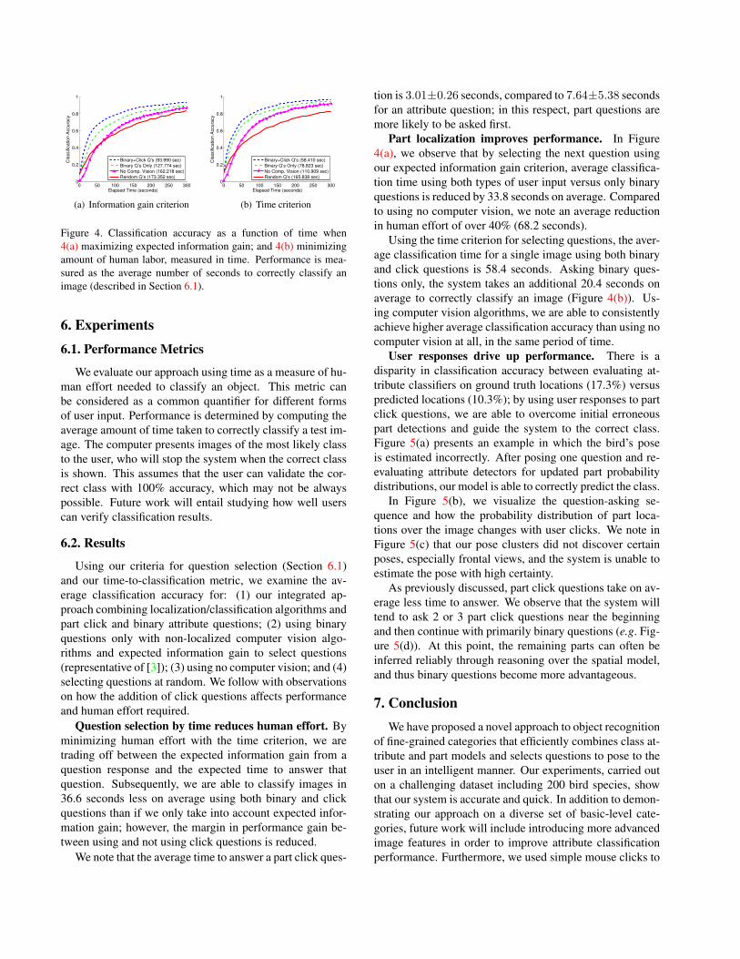
Figure 4. Classification accuracy as a function of time when
4(a) maximizing expected information gain; and 4(b) minimizing
amount of human labor, measured in time. Performance is mea-
sured as the average number of seconds to correctly classify an
image (described in Section 6.1).
6. Experiments
6.1. Performance Metrics
We evaluate our approach using time as a measure of hu-
man effort needed to classify an object. This metric can
be considered as a common quantifier for different forms
of user input. Performance is determined by computing the
average amount of time taken to correctly classify a test im-
age. The computer presents images of the most likely class
to the user, who will stop the system when the correct class
is shown. This assumes that the user can validate the cor-
rect class with 100% accuracy, which may not be always
possible. Future work will entail studying how well users
can verify classification results.
6.2. Results
Using our criteria for question selection (Section 6.1)
and our time-to-classification metric, we examine the av-
erage classification accuracy for: (1) our integrated ap-
proach combining localization/classification algorithms and
part click and binary attribute questions; (2) using binary
questions only with non-localized computer vision algo-
rithms and expected information gain to select questions
(representative of [3]); (3) using no computer vision; and (4)
selecting questions at random. We follow with observations
on how the addition of click questions affects performance
and human effort required.
Question selection by time reduces human effort. By
minimizing human effort with the time criterion, we are
trading off between the expected information gain from a
question response and the expected time to answer that
question. Subsequently, we are able to classify images in
36.6 seconds less on average using both binary and click
questions than if we only take into account expected infor-
mation gain; however, the margin in performance gain be-
tween using and not using click questions is reduced.
We note that the average time to answer a part click ques-
tion is 3.01±0.26 seconds, compared to 7.64±5.38 seconds
for an attribute question; in this respect, part questions are
more likely to be asked first.
Part localization improves performance. In Figure
4(a), we observe that by selecting the next question using
our expected information gain criterion, average classifica-
tion time using both types of user input versus only binary
questions is reduced by 33.8 seconds on average. Compared
to using no computer vision, we note an average reduction
in human effort of over 40% (68.2 seconds).
Using the time criterion for selecting questions, the aver-
age classification time for a single image using both binary
and click questions is 58.4 seconds. Asking binary ques-
tions only, the system takes an additional 20.4 seconds on
average to correctly classify an image (Figure 4(b)). Us-
ing computer vision algorithms, we are able to consistently
achieve higher average classification accuracy than using no
computer vision at all, in the same period of time.
User responses drive up performance. There is a
disparity in classification accuracy between evaluating at-
tribute classifiers on ground truth locations (17.3%) versus
predicted locations (10.3%); by using user responses to part
click questions, we are able to overcome initial erroneous
part detections and guide the system to the correct class.
Figure 5(a) presents an example in which the bird’s pose
is estimated incorrectly. After posing one question and re-
evaluating attribute detectors for updated part probability
distributions, our model is able to correctly predict the class.
In Figure 5(b), we visualize the question-asking se-
quence and how the probability distribution of part loca-
tions over the image changes with user clicks. We note in
Figure 5(c) that our pose clusters did not discover certain
poses, especially frontal views, and the system is unable to
estimate the pose with high certainty.
As previously discussed, part click questions take on av-
erage less time to answer. We observe that the system will
tend to ask 2 or 3 part click questions near the beginning
and then continue with primarily binary questions (e.g. Fig-
ure 5(d)). At this point, the remaining parts can often be
inferred reliably through reasoning over the spatial model,
and thus binary questions become more advantageous.
7. Conclusion
We have proposed a novel approach to object recognition
of fine-grained categories that efficiently combines class at-
tribute and part models and selects questions to pose to the
user in an intelligent manner. Our experiments, carried out
on a challenging dataset including 200 bird species, show
that our system is accurate and quick. In addition to demon-
strating our approach on a diverse set of basic-level cate-
gories, future work will include introducing more advanced
image features in order to improve attribute classification
performance. Furthermore, we used simple mouse clicks to

Pose body breast tail head throat
Facing_
right
Facing_
left
Initial
predicted
part locations
Q1: Click on the
beak (3.200 s)
Pose body breast tail head throat
Facing_
right
Facing_
left
. .
Initial predicted
part locations
Ground truth
part locations Pose tail breast l. eye r. eye beak breast
Head_turn
ed_right
Fly_swim_
to_right
Fly_swim_
to_left
tail breast l. eye r. eye beak breast
Initial pred. part locations
Orange-Crowned Warbler? no
Q1: Is the throat yellow?
no (4.547 s) Great Crested Flycatcher? no
Mourning Warbler? yes
Q2: Click on the tail (2.043 s)
Q3: Click on the head (2.452 s)
Yellow Bellied Flycatcher? no
Initial pred. part locations
Prothonotary Warbler? no
Q1: Click on the
belly (4.357 s)
Yellow-headed Blackbird? yes
(a) (b) (d)
(c)
Figure 5. Four examples of the behavior of our system. 5(a): The system estimates the bird pose incorrectly but is able to localize the
head and upper body region well, and the initial class prediction captures the color of the localized parts. The user’s response to the first
system-selected part click question helps correct computer vision. 5(b): The bird is incorrectly detected, as shown in the probability maps
displaying the likelihood of individual part locations for a subset of the possible poses (not visible to the user). The system selects “Click
on the beak” as the first question to the user. After the user’s click, the other part location probabilities are updated and exhibit a shift
towards improved localization and pose estimation. 5(c): Certain infrequent poses (e.g. frontal views) were not discovered by the initial
off-line clustering (see Figure 2(a)). The initial probability distributions of part locations over the image demonstrate the uncertainty in
fitting the pose models. The system tends to fail on these unfamiliar poses. 5(d): The system will at times select both part click and binary
questions to correctly classify images.
designate part locations, and it would be of interest to inves-
tigate whether asking the user to provide more detailed part
and pose annotations would further speed up recognition.
8. Acknowledgments
The authors thank Boris Babenko, Ryan Farrell, Kristen
Grauman, and Peter Welinder for helpful discussions and
feedback, as well as Jitendra Malik for suggesting time-to-
decision as a relevant performance metric. Funding for this
work was provided by the NSF GRFP for CW under Grant
DGE 0707423, NSF Grant AGS-0941760, ONR MURI
Grant N00014-08-1-0638, ONR MURI Grant N00014-06-
1-0734, and ONR MURI Grant 1015 G NA127.
References
[1] P. Belhumeur et al. Searching the world’s herbaria: A system
for visual identification of plant species. In ECCV, 2008.
[2] L. Bourdev and J. Malik. Poselets: Body part detectors
trained using 3d human pose annotations. In ICCV, 2009.
[3] S. Branson et al. Visual recognition with humans in the loop.
In ECCV, 2010.
[4] I. Endres et al. The benefits and challenges of collecting
richer object annotations. In ACVHL, 2010.
[5] A. Farhadi, I. Endres, and D. Hoiem. Attribute-centric recog-
nition for cross-category generalization. In CVPR, 2010.
[6] A. Farhadi, I. Endres, D. Hoiem, and D. Forsyth. Describing
objects by their attributes. In CVPR, 2009.
[7] L. Fei-Fei, R. Fergus, and P. Perona. A bayesian approach
to unsupervised one-shot learning of object categories. In
ICCV, volume 2, page 1134, 2003.
[8] P. Felzenszwalb et al. A discriminatively trained, multiscale,
deformable part model. In CVPR, 2008.
[9] P. Felzenszwalb and D. Huttenlocher. Efficient matching of
pictorial structures. In CVPR, 2000.
[10] A. Holub et al. Hybrid generative-discriminative visual cat-
egorization. ICCV, 77(1-3):239–258, 2008.
[11] N. Kumar et al. Attribute and simile classifiers for face veri-
fication. In ICCV, 2009.
[12] C. Lampert et al. Learning to detect unseen object classes by
between-class attribute transfer. In CVPR, 2009.
[13] S. Lazebnik et al. A maximum entropy framework for part-
based texture and object recognition. In ICCV, 2005.
[14] Martınez-Munoz et al. Dictionary-free categorization of very
similar objects via stacked evidence trees. In CVPR, 2009.
[15] M. Nilsback and A. Zisserman. Automated flower classifica-
tion over a large number of classes. In ICCVGIP, 2008.
[16] M. Stark, M. Goesele, and B. Schiele. A shape-based object
class model for knowledge transfer. In ICCV, 2010.
[17] I. Tsochantaridis, T. Joachims, T. Hofmann, and Y. Altun.
Large margin methods for structured and interdependent out-
put variables. JMLR, 6(2):1453, 2006.
[18] C. Wah, S. Branson, P. Welinder, P. Perona, and S. Belongie.
The Caltech-UCSD Birds-200-2011 Dataset. FGVC, 2011.
[19] M. Waite. http://www.whatbird.com/.
[20] G. Wang and D. Forsyth. Joint learning of visual attributes,
object classes and visual saliency. In ICCV, 2009.
[21] M. Weber, M. Welling, and P. Perona. Unsupervised learning
of models for recognition. In ECCV, Dublin, Ireland, 2000.
[22] P. Welinder et al. Caltech-UCSD Birds 200. Technical Re-
port CNS-TR-2010-001, Caltech, 2010.
[23] Y. Yang and D. Ramanan. Articulated Pose Estimation using
Flexible Mixtures of Parts. In CVPR, 2011.
Related Documents