Multi-Scale Patterns of Eastern Milksnake (Lampropeltis ...

Multi-Scale Patterns of Eastern Milksnake (Lampropeltis triangulum) Habitat Selection and

Behavioural Responses to Habitat Fragmentation

by

Marcus Maddalena

A thesis

presented to the University of Waterloo

in fulfillment of the

thesis requirements for the degree of

Master of Environmental Studies

in

Social and Ecological Sustainability

Waterloo, Ontario, Canada, 2018

© Marcus Maddalena 2018

ii

Authors Declaration

I hereby declare that I am the sole author of this thesis. This is a true copy of the thesis, including

any required final revisions, as accepted by my examiners.

I understand that my thesis may be made electronically available to the public.

iii

Abstract

The decline of species with specific habitat needs can be attributed to human caused habitat

destruction and fragmentation. This is particularly concerning for reptiles, as they are often unable

to adapt to modified landscapes. The eastern milksnake (Lampropeltis triangulum) represents the

rare case of a species at risk that has persisted both in disturbed and undisturbed landscapes

throughout its historic Canadian range. However, a lack of contemporary occurrence data makes

it difficult to assess the impact of perceived threats on the species, or devise effective conservation

strategies. Here, I aim to quantify milksnake habitat selection and potential behavioural adaptation

in response to human development at multiple spatial scales. Specifically, I address the questions

1) Do milksnakes modify behaviours (home range size, movement rates) in response to human

modified landscapes? 2) Which habitats are milksnakes selecting for at the home range scale, and

within the home range, which microhabitat features are selected for? And 3) How does landscape

scale habitat fragmentation impact milksnake distribution? I used radio telemetry to track 17

individuals between 2015 and 2017 in Rouge National Urban Park, and used a large scale

coverboard survey to generate occurrence records across the Credit Valley and Toronto Region

Conservation Authority Management Areas. Using this data, I analyzed movement rates, assessed

the degree of road avoidance, determined home range sizes, and compared these metrics to a

natural site. I then analyzed home range scale habitat selection, and determined which

microhabitats features are selected for within home ranges. Using occurrence data, I determined

best predicted landscape scale habitat for milksnakes, and compared this to a generalist species.

Results indicate that milksnakes are modifying behaviours in urban landscapes, as they have

significantly higher movement rates and avoid road crossings. Milksnakes are also avoiding human

modified landcover types (urban area and agriculture) at all scales. At the home range and

iv

microhabitat scales, milksnakes are selecting a variety of open habitats with abundant cover, while

selection at the landscape scale favours large habitat patches. In order to conserve snake

populations, I recommend that conservation of large natural areas and the establishment of

corridors connecting them are prioritized.

v

Acknowledgements

I would like to thank my advisor Dr. Brad Fedy for his guidance throughout the years and for

presenting me with the opportunity to be involved in this project. From my time as an

undergraduate on, Brad has mentored me and given me opportunities to become a better ecologist.

I would also like to thank Dr. Jeff Row, who was there to help at every step throughout this project,

whether that meant sitting down with me and working through code or spending days in the field.

I would also like to thank Sarantia Katsaras, whose commitment to the project was more than

I could have hoped for, and Catherine Falardeau Marcoux, who set up a large portion of the project.

Many volunteers also helped make this project possible, and I would be remiss not to mention

them. Thank you, Marten, Kaas (who sacrificed many days of his own research), Charisa Gerow,

Justin Maddalena, Greg Misner, and Ben North for donating your time and effort.

I must also thank the Toronto Zoo, specifically Paul Yannuzzi, Andrew Lentini, and the entire

veterinary staff who donated their time to ensure this project was completed successfully.

Further thanks go to the funders who made this project possible, specifically Parks Canada and

the Species at Risk Fund for Ontario.

I could not have completed my schooling with the support from my parents. Despite not always

understanding my work or motivations, you encouraged me to pursue whatever education I saw

fit.

I am also indebted to Alex Robinson for her ongoing encouragement and support despite my

busy schedule. I intend to make it up to you by finally enjoying weekends spent together.

vi

Table of Contents

Authors Declaration ........................................................................................................................ ii

Abstract .......................................................................................................................................... iii

Acknowledgements ......................................................................................................................... v

List of Tables .................................................................................................................................. x

1 General Introduction ................................................................................................................ 1

2 Review of the Literature .......................................................................................................... 3

2.1 A Brief History of Niche Theory ..................................................................................... 3

2.2 Defining Habitat and Associated Terms .......................................................................... 5

2.3 Urban Ecology – An Emerging Discipline ...................................................................... 7

2.4 Herpetofauna and Susceptibility to Human Impacts ........................................................ 8

2.5 Study Species – The Eastern Milksnake ........................................................................ 10

2.6 Thesis Outline and Research Questions ......................................................................... 12

2.7 Study Area ...................................................................................................................... 13

3 Habitat Selection and Behavioural Modifications by Milksnakes in Response to Habitat

Fragmentation ............................................................................................................................... 14

3.1 Introduction .................................................................................................................... 14

3.2 Methods .......................................................................................................................... 17

3.2.1 Study Area .............................................................................................................. 17

3.2.2 Difference in Home Range Size Between Sites ...................................................... 19

3.2.3 Differences in Movement Rates Between Sites ...................................................... 20

3.2.4 Road Avoidance in A Fragmented Landscape ........................................................ 20

3.2.5 Habitat Selection at the Home Range Scale ........................................................... 21

3.2.6 Habitat Selection at the Individual Location .......................................................... 22

3.3 Results ............................................................................................................................ 24

3.3.1 Comparison of Home Range Sizes Between Sites ................................................. 24

3.3.2 Differences in Movement Rates Between Sites ...................................................... 25

3.3.3 Road Avoidance in A Fragmented Landscape ........................................................ 26

3.3.4 Habitat Selection at the Home Range Scale in Rouge National Urban Park .......... 26

3.3.5 Habitat Selection at the Individual Location in Rouge National Urban Park ......... 27

3.4 Discussion ...................................................................................................................... 29

vii

4 Assessing and Comparing Best Predicted Habitat of a Generalist and a Specialist Snake

Species Along an Urban Gradient................................................................................................. 34

4.1 Introduction .................................................................................................................... 34

4.2 Methods .......................................................................................................................... 36

4.2.1 Study Area .............................................................................................................. 36

4.2.2 Occurrence and Absence Locations ........................................................................ 38

4.2.3 Covariate Development .......................................................................................... 39

4.2.4 Model Development and Selection ......................................................................... 40

4.2.5 Model Evaluation and Comparison ........................................................................ 41

4.3 Results ............................................................................................................................ 42

4.3.1 Model Selection ...................................................................................................... 42

4.3.2 Resource Selection Functions ................................................................................. 43

4.3.3 Species Comparisons .............................................................................................. 43

4.4 Discussion ...................................................................................................................... 50

5 Conclusions ........................................................................................................................... 54

6 References ............................................................................................................................. 56

7 Appendix 1: Supplementary Material .................................................................................... 66

viii

List of Figures

Figure 1. Maps of Rouge National Urban Park and Queens University Biology Station study areas

created by placing 1km radial buffers around all occurrence locations generated using radio

telemetry. Contrasting land used surrounding the study areas are apparent here. ................. 18

Figure 2. Box plots showing distance moved per day for individuals at Rouge National Urban Park

and Queens University Biology Station, and home range size of male and female milksnakes

in each study area. ................................................................................................................. 25

Figure 3. Standardized coefficients of top model and 97.5% confidence intervals potentially

contributing to the differences between used and available locations at the home range scale

controlling for individual variation as a random effect. ........................................................ 26

Figure 4. Standardized coefficients of the top model and 97.5% confidence intervals contributing

to the difference between used and available locations. ........................................................ 28

Figure 5. Map of the study area boundary is indicated by the black line. Snake survey locations

(i.e., coverboards) are indicated by the red circles. Study area boundary was defined by

combining the Toronto Region Conservation Authority and Credit Valley Conservation

Authority boundaries. Major highways, cities, and natural areas (in green) can also be seen in

the background layer. ............................................................................................................ 37

Figure 6. Coefficient estimates from gartersnake top model. Coefficients for milksnakes, produced

using the landcover covariates from the gartersnake top model, are also displayed. ............ 45

Figure 7. Coefficient estimates from milksnake top model. Coefficients for gartersnakes, produced

using the landcover covariates from the milksnake top model, are also displayed. .............. 46

Figure 8. Responses to human modified landcover types by milksnakes (left) and gartersnakes

(right) and the data used to generate response curves and associated standard error (shown in

grey). ...................................................................................................................................... 47

Figure 9. Resource selection functions for eastern milksnake and eastern gartersnake including all

occurrence locations (black) used in model development and coverboard locations (red) used

to gather occurrence records. Scale bars represent increasing relative probability of

occurrence. ............................................................................................................................. 48

Figure 10. Areas with high likelihood of occurrence for gartersnake and milksnake (blue), or one

of these species (red) within the study area. Areas with low likelihood of occurrence for both

species are not highlighted. ................................................................................................... 49

ix

Figure 11. Map showing contemporary (post-2000) occurrence of milksnakes in the Credit Valley

and Toronto Region Conservation Authority management areas. It is evident that current

distribution is limited to larger natural areas, with some occurrence records present in small,

more urban natural areas. ....................................................................................................... 66

Figure 12. Map showing historic occurrence records (pre-2000) of milksnakes in the Credit Valley

and Toronto Region Conservation Authority management areas. The background layer used

is contemporary, and highlights the amount of urban development through areas of historic

occurrence. ............................................................................................................................. 67

Figure 13. Sample plots of individuals whose home range did and did not reach an asymptote.

Plots were created by plotting home range size against number of relocations. Those that

reached an asymptote were thought to have accessed their entire home range during the study

period, and were included in home range analysis. ............................................................... 68

Figure 14. Example of used (white) and available (red) plots used in determine home range scale

habitat selection, including roads. The central point represents this individual’s hibernation

site, and the large circle is a radial plot of the maximum distance travelled from the hibernation

site. Random plots were generated in an area theoretically accessible to the individual based

on maximum dispersal distance from the hibernaculum. ...................................................... 69

Figure 15. Mean covariates for each individual used in modelling home range habitat selection.

Presence and absence locations are shown separately here for all seven landcover covariates

used in modelling................................................................................................................... 70

x

List of Tables

Table 1. Landcover layers used in modelling home range scale habitat selection by eastern

milksnakes in Rouge National Park and the justification for including layers. .................... 22

Table 2. Names and definitions of variables used in modelling habitat selection at individual

locations in Rouge National Urban Park.e ............................................................................ 23

Table 3. Number of individual milksnakes tracked by site and sex, including metrics associated

with the number of relocation at Rouge National Urban Park and Queens University Biology

Station. ................................................................................................................................... 24

Table 4. All candidate producing ∆AIC values <2 for milksnake habitat covariates at the home

range scale ............................................................................................................................. 27

Table 5. All candidate producing ∆AIC values <4, and potentially contributing to habitat selection

by milksnakes at the exact location. ...................................................................................... 28

Table 6. Development of landcover layers used in the development of models and resource

selection functions, including landcover types used in building each layer (AAFC, 2014).

Denotation by ǂ indicates a human-modified landcover type. ............................................... 39

Table 7. Summary of occurrence used in modelling and to develop resource selection functions.

............................................................................................................................................... 42

Table 8.Milksnake and gartersnake model tables including all candidate producing ∆AIC values

<2, and potentially contributing to occurrence locations. ..................................................... 43

1

1 General Introduction

Pressures on wildlife in the form of human-driven habitat loss and fragmentation are the

leading causes of contemporary extinction events globally (Fahrig, 1997; Gill, Sutherland, &

Watkinson, 1996; Hoekstra, Boucher, Ricketts, & Roberts, 2005; Krauss et al., 2010). Wildlife

species demonstrate incredible variation in their ability to tolerate human disturbances, as species

respond to different types of disturbances at different scales (Bender, Contreras, & Fahrig, 1998;

Cagnolo, Valladares, Salvo, Cabido, & Zak, 2009). Species that thrive in these fragmented

landscapes typically utilize a combination of small habitat patches and surrounding developed

areas (Gill et al., 1996). Alternatively, species with specific habitat needs and several species at

risk often experience further decline and displacement due to anthropogenic disturbances, which

may result in a low likelihood of long term persistence on the landscape (Ewers & Didham, 2006;

Kerr & Deguise, 2004). Understanding how species respond to anthropogenic pressures is

therefore essential to predict global biodiversity trends and develop effective conservation

strategies. However, responses to habitat fragmentation and loss are not linear, meaning responses

to these threats occur along a gradient, with different species being impacted at varying scales both

spatially and temporally.

The eastern milksnake (Lampropeltis triangulum) represents the rare case of a species at risk

that has persisted in both disturbed and undisturbed regions throughout its historic range.

Recognized threats for milksnakes include road or rail mortality, habitat loss from urban

development, intensive agriculture, and persecution due to misidentification as a poisonous species

(COSEWIC, 2014). These recognized threats are concerning throughout the species Canadian

range due to the ongoing and intensive development.

2

Current knowledge of milksnake habitat selection is limited to a study on a large piece of

intact habitat ( Row & Blouin-Demers, 2006b, 2006c). This leaves a knowledge gap regarding the

species ecology in disturbed area, as it remains uncertain how disturbance influences available

habitat, behavioural ecology, and habitat selection. To fill this knowledge gap, this thesis

systematically quantifies milksnake habitat selection and behavioural modification at multiple

spatial scales in a developed region.

3

2 Review of the Literature

2.1 A Brief History of Niche Theory

Niche theory involves the study and formal definition of the mechanisms driving wildlife

occupancy of environmental and geographic space. Scientists have long attempted to explain these

mechanisms, which has led to the development of competing definitions of niche and many sub

theories (Schnieder & Willig, 2005). Niche theory was originally developed at two separate sub-

theories focused on place of a species (Grinnell, 1917) and role of a species (Elton, 1927) in

explaining distribution (Schnieder & Willig, 2005; Soberón, 2007). Grinellean niche considers a

species occupancy of geographic space a direct response to a narrow range of environmental

conditions, defined by non-interactive environmental variables on coarse scales (Grinnell, 1917,

Soberón, 2007). Eltonian niche considers competition for resources between species at local scales

as the primary driver of occupancy of environmental space (Elton, 1927; Soberón, 2007).

In an attempt to clarify these terms, Hutchinson (1957) proposed that a species niche can

be defined quantitatively as an n-dimensional hypervolume of factors influencing persistence of a

given species (Hutchinson, 1957; Schnieder & Willig, 2005). Fundamental niche of a species is

represented by all of the points in this n-dimensional space that meet the species requirements,

theoretically allowing it to exist (Hutchinson, 1957). The inherent complexity of ecological

systems and biotic interactions do not necessarily allow access to all points within this space.

Realized niche is then the n-dimensional space that a species can occupy based on competition

with interacting species, and dispersal ability (Hutchinson, 1957; Schnieder & Willig, 2005).

The development of more advanced quantitative methods in ecology has since allowed

Hutchinson’s niche concept to be challenged statistically (P. H. Harvey, Colwell, Silvertown, &

May, 1983; Schnieder & Willig, 2005; Simberloff, 1978). Simberloff (1978) used a null model to

4

test whether colonization based on species interactions differs from random chance, finding that

the null model preformed quite well with the caveat that vertebrate distribution remains influenced

by diffuse competition (P. H. Harvey et al., 1983). Despite the performance of thoughtfully

parameterized null models, a number of competing hypotheses and models exist to explain wildlife

occurrence patterns (P. H. Harvey et al., 1983).

There has since been robust development in ecological modelling and the ability to address

many competing hypotheses and predict species distributions across landscapes, though clarity is

often lacking as to whether these models explain distribution or niche (Elith & Leathwick, 2009;

Raudsepp-Hearne & Peterson, 2016; Soberón, 2007). Models explaining niche account for

interactions between species, while models explaining distribution are based on environmental

data (Elith & Leathwick, 2009).To clarify what a given model type explains, it is important to note

the distinction between mechanistic models predicting niche and correlative models predicting

distribution (Elith & Leathwick, 2009; Kearney & Porter, 2009; Soberón, 2007). Mechanistic

models include information regarding links between organisms and their environment (such as

behavioural, morphological, and physical traits) (Kearney & Porter, 2009). As a consequence,

mechanistic models are able to provide outputs which indirectly represent many processes

(Kearney & Porter, 2009). However, the data regarding mechanistic links between organisms and

their environments is only available for well studied taxa (Kearney & Porter, 2009; Soberón,

2007). Correlative models are more widely applicable probability based models related to broad

scale habitat parameters and requiring decidedly less detailed species data (Elith & Leathwick,

2009). The term correlative models is applied to describe many distribution modelling approaches

also referred to as: bioclimatic models, climate envelopes, ecological niche models, species

distribution models, range maps, and resource selection functions (Elith & Leathwick, 2009). The

5

lack of information regarding biotic interactions in correlative models raises the question of

whether they examine realized or fundamental niche. Guisan and Zimmermann (2000) argue that

models based on field data depict the realized niche, as occurrence observations are obtained in

the form of occupied animal locations which are based on biotic interaction with other species.

2.2 Defining Habitat and Associated Terms

Models predicting a species occurrence based on habitat are subject to the assumption that

if an animal uses a habitat type disproportionately to its availability, then that habitat is biologically

relevant (Aebischer, Robertson, & Kenward, 1993; Johnson, 1980). This assumption is widely

accepted, but the definitions of habitat and related terms vary throughout the literature (Hall,

Krausman, & Morrison, 1997). For consistency in this study, we adopt definitions for habitat and

associated terms based reviews of previous use in the literature (Krausman, 1999; Lele, Merrill,

Keim, & Boyce, 2013). Habitat is defined as the resources and conditions present in an area that

lead to occupancy by an organism (Krausman, 1999). These resources include factors (such as

food, cover, water) that are required for a species survival and reproduction, including seasonally

used migration and dispersal corridors (Krausman, 1999; Leopold, 1933). For studies that include

distribution modelling approaches, the distinction must also be made between resource units and

resource types (Lele et al., 2013). Resource units are items available for consumption distributed

through the landscape, or pixels imposed on a landscape to represent habitat (Lele et al., 2013). In

this study, I use resource units in the form of pixels imposed on the landscape to represent habitat

types, and as a consequence the terms habitat type and resource unit are used somewhat

interchangeably. If multiple resource units have the same attributes, they are considered the same

resource type. (Lele et al., 2013).

Habitat use is the way these resources are used (for forage, cover, nesting, or a variety of

other life history traits), though a given resource is not always used exclusively for one life history

6

trait (Krausman, 1999). Likewise, resource units are considered used if they subject to investment

by an animal for perceived benefit (Buskirk & Millspaugh, 2006; Lele et al., 2013). Habitat use is

subject to seasonal variation based on life history traits and dispersal (Elith & Leathwick, 2009;

Krausman, 1999; Peterson, 2006). For example, an animals seasonal breeding sites, hibernation

sites, forage sites, and corridors connecting them all represent used habitat. Without data that

encompasses multiple seasons, it may not be possible to identify habitat use associated with all

important life history traits.

Habitat use does not necessarily imply habitat selection as an animal may use one habitat

or resource unit as a means of accessing another (Krausman, 1999). Habitat selection refers to the

use of a habitat by an animal if that habitat it is encountered (Lele et al., 2013). Habitat selection

is relatively intuitive to understand as a binary term, with an encountered habitat considered used

or unused (Boyce, Vernier, Nielsen, & Schmiegelow, 2002; Lele et al., 2013). Probability of

selection is then the probability that a given habitat type will be used if encountered, based solely

on the habitat type and its ability to satisfy a life history trait (Lele et al., 2013). Probability of use

refers to a single instance of use in a given habitat type and is limited by whether that habitat can

be accessed (Lele et al., 2013). If a habitat type is selected for but is inaccessible, then it will have

a low probability of use (Lele et al., 2013).

Habitat selection is a hierarchical process which has been suggested to occur at four distinct

spatial scales (Johnson, 1980). First order selection is the physical or geographic range of a species,

which dictates second order selection of a home range (Johnson, 1980). Third order selection is

the use of various habitat types and sites within the home range, while fourth order selection

involves the procurement of food items or other benefit from those sites (Johnson, 1980).

7

These orders of habitat selection are relatively intuitive to understand, and assessing habitat

selection at an appropriate spatial scale has long been considered important in quantifying wildlife

habitat, however, all habitat at a given scale is not equally accessible to an individual (Johnson,

1980). While it is clear that appropriate scales must also be selected, a species’ ability to access

habitat at a given scale must be considered. This requires researchers to develop an understanding

of species’ ability to move through a given landscape. Ability to access suitable habitat patches is

often limited in urban landscapes.

2.3 Urban Ecology – An Emerging Discipline

Urban ecology is a relatively new sub-discipline of ecology that is generally thought to have

begun in the 1970’s (McDonnell, 2011; McDonnell & Pickett, 1993). The need to consider urban

ecology as a distinct sub-discipline emerged from the recognition that human development

fundamentally changes ecosystems by fragmenting and removing habitat (Deelstra, 1988;

McDonnell, 2011; Niemela, 2000). These processes are especially intensive in urban areas relative

to rural areas, as natural landscapes are often removed rather than altered. Urban ecology has then

emerged partially out of necessity, as rapid human population growth has left few ecosystems

unaltered. Early definitions of urban ecology focused on the integration of: 1) natural sciences, 2)

engineering/urban planning, and 3) social sciences (Deelstra, 1988; McDonnell, 2011). However,

more recent work has stated that social sciences and natural sciences within urban ecology should

be considered as distinct fields of study, with the social component focussing in human health as

it related to the environment and the natural component focusing on biological processes (Niemela,

2000). These fields fall under the umbrella of urban ecology as long as they occur in urban areas

where 85% of the population lives is non-rural (Niemela, 2000; Rebele, 1994).

8

Ecological studies in urban areas typically focus on the ability of wildlife to access habitat,

patch characteristics, or invasion by invasive species (Niemela, 2000; Rebele, 1994). In urban

areas, the ability of wildlife to access suitable habitat is negatively impacted by high intensity

roads, dense development, and a lack of corridors (Gill et al., 1996; McDonnell & Pickett, 1993;

McKinney, 2006). Additionally, decreases in patch size and increases in disturbance limit the

ability of wildlife to access suitable habitat and persist in urban landscapes (Hagen et al., 2012).

The theory of island biogeography has historically been applied to understand patch characteristics

in urban landscapes, by treating isolated urban habitat patches in the same way as islands (Davis

& Glick, 1978; MacArthur & Wilson, 1967). Fragmented patch characteristics alter species

composition to favour invasive species and generalists (Hagen et al., 2012; Randa & Yunger,

2006). Species richness is often high in urban ecosystems due to a variety of edges and

microhabitats, but this does not necessarily indicate a healthy system as the function that the

historic state of the system may not be replicated (McDonnell, 2011; Niemela, 2000; Rebele,

1994). Recent work has shown that urbanization and the impacts on wildlife occur along a gradient

from rural to urban (Randa & Yunger, 2006). Still, wildlife species are limited by patch size and

their ability to access suitable habitat in urban areas.

2.4 Herpetofauna and Susceptibility to Human Impacts

Herpetofauna are especially susceptible to the negative impacts of habitat loss and

fragmentation (Gibbons et al., 2000). They are a relatively slow moving group of species often

with specific habitat needs (Gibbons et al., 2000; Reading et al., 2010). Though reptiles and

amphibians are both considered herpetofauna, they are morphologically and behaviourally distinct

(Gibbons et al., 2000; Reading et al., 2010). Reptiles generally have much larger home ranges and

higher movement rates than amphibians, which makes them more susceptible to negative impacts

9

of habitat fragmentation (Gibbons et al., 2000). This thesis is concerned with snakes, but it is worth

noting that amphibians face many of the same pressures and are subject to the same trends of

decline (Gibbons et al., 2000)

In recent years, snake populations have experienced a marked decline globally across habitat

types and species (Mullin & Seigel, 2009; Reading et al., 2010). It is possible that global population

decline has been occurring for much longer, but with few long term snake studies on which

population can be assessed, this remains an assumption (Reading et al., 2010). Snakes are often

top predators so a decline in their numbers can have serious consequences for ecosystems (Reading

et al, 2010).

The potential impact of habitat loss on snakes is relatively simple to understand. If important

habitat or habitat features (such as hibernation sites) are removed from a landscape, the animal

will not persist if it cannot access these features elsewhere (Mullin & Seigel, 2009; Reading et al.,

2010). To contrast this, the effects of habitat fragmentation are often subtle. Perhaps the most

obvious of these impacts is road mortality, which is higher in fragmented areas ( Row, Blouin-

Demers, & Weatherhead, 2007). Fragmentation by roads and development can also lead to altered

home ranges, as some species are unwilling or unable these features to access former home range

areas (Klingenbock, Osterwalder, & Shine, 2000). In the long term, these factors can lead to

behavioural changes, reducing gene flow between population clusters (Clark, Brown, Stechert, &

Zamudio, 2010; Klingenbock et al., 2000; Shepard, Kuhns, Dreslik, & Phillips, 2008). When

habitat patches are not suitable large to sustain populations, regional extirpation or extinction can

occur (Germaine & Wakeling, 2001; Rudolph, Burgdorf, Conner, & Schaefer, 1999).

10

2.5 Study Species – The Eastern Milksnake

The eastern milksnake (Lampropeltis triangulum) represents the rare case of a relatively long

lived species at risk snake that has persisted in both disturbed and undisturbed areas throughout its

range. The species range extends throughout eastern North America, reaching its northern limits

in Ontario and southern Quebec’s Great Lakes/St. Lawrence and Carolinian regions (COSEWIC,

2014; Ruane, Bryson, Pyron, & Burbrink, 2014). Despite historic occurrence through large parts

of Canada’s most populated regions, little contemporary information is available on the species in

this area, with most of the existing knowledge coming from one study in a natural landscape

(COSEWIC, 2014; Row & Blouin-Demers, 2006b, 2006c). Limited information on population

size and distribution has contributed to the species national listing as Special Concern (COSEWIC,

2014). Current knowledge on the extent of Canada’s milksnake population comes primarily from

occurrence records submitted to the Natural Heritage Information Centre (NHIC). These records

show that developed regions are dominated by historic records with relatively few observations

post 2000. This is evident around Toronto, Ontario, as populations persist throughout the region

but are thought to have been in decline for over 30 years (COSEWIC, 2014). This decline has not

been confirmed, as no studies on population size or formal survey for the species has taken place

prior to 2011.

Milksnakes are historically associated with low intensity agricultural areas, even owing their

name to occurrence in cattle barns (COSEWIC, 2014; Lentini, Yannuzzi, Phillips, & Johnson,

2015). Human features in these low intensity agricultural landscapes and small mammal borrows

are important habitat features for milksnakes for a variety of life history traits (such as feeding,

hibernation, shelter). Abundance of small mammals, the primary food source of adult milksnakes,

is typically high in these habitats (COSEWIC, 2014; Lentini et al., 2015). Barns and foundations

also provide readily accessible and highly suitable hibernation sites (COSEWIC, 2014; Lentini et

11

al., 2015). The preservation of these human made habitat features is then important to conserve

the species (Lentini et al., 2015). Milksnakes are also a very cryptic species, rarely basking in the

open and preferring to thermoregulate using ambient heat on the underside of exposed objects or

vegetation (COSEWIC, 2014).

Milksnakes are regarded as a generalist species throughout their range based on their

occurrence in many habitat types. I argue that the Canadian population should be considered

specialists, and that previous conclusions about habitat specialization have been made at an

inappropriate spatial scale. As the Canadian population of milksnakes is at the species northern

range limit, thermal quality is much lower than elsewhere in the species range. Snakes occurring

in high thermal quality habitat are able to bask indiscriminately, which allows for use of a broad

range of habitat types (Ralph Gibson & Bruce Falls, 1979). At their northern range limits, snakes

are known to select habitat based on thermal quality (Goulet, Litvaitis, & Marchand, 2015; Row

& Blouin-Demers, 2006b, 2006c). Row & Blouin-Demers (2006b, 2006c) found milksnakes to

have strong association with fields and open habitats in close proximity to forest edges. The use

of open habitats by milksnakes is consistent across seasons ( Row & Blouin-Demers, 2006c) In

these thermally challenging habitats, milksnakes alter seasonal basking behaviour for thermal

benefit rather than altering habitat selection, spending longer periods of time basking as

temperature decreases ( Row & Blouin-Demers, 2006b). It is clear that current knowledge

demonstrates that milksnakes in Canada select few high quality thermal quality habitats within

their home range. In this thesis, I consider milksnakes to be specialists of fields and open habitats

near forest edges, based on the availability of high quality thermal sites and potential prey in these

areas.

12

2.6 Thesis Outline and Research Questions

This thesis aims to quantify milksnake habitat selection and potential behavioural adaptation

in response to human development at multiple spatial scales by answering the following questions:

1) Do milksnakes modify behaviours (home range size, movement rates) in response to human

modified landscapes?; 2) Which habitats are milksnakes selecting for at the home range scale and

within the home range, which microhabitat features are selected for?; And 3) How does landscape

scale habitat fragmentation impact milksnakes distribution?

Questions 1 and 2 are addressed in chapter 3, where I compare movement rates and home

range size between a disturbed and natural site to determine the degree to which habitat loss and

fragmentation can influence them. Additionally, I quantify second and third order habitat selection

within the disturbed site to understand which landcover types and micro-habitat features are

selected for in a developed area. Overall this chapter provides an understanding of behavioural

adaptations and habitat selection by milksnakes in response to disturbance.

Question 3 is addressed in Chapter 4 where I compare predicted landscape scale distribution

of milksnakes to a generalist species. In this chapter, I analyze habitat selection across scales for

both species at the landscape scale and investigate the strength of selection and avoidance for

multiple, biologically-relevant, landcover types. I then develop spatially-explicit predictions of the

relative probability of occupancy for each species and created an overlay of best predicted habitat

to understand the potential for multi-species conservation prioritization. Overall, this chapter

provides a deeper understanding of the ways in which landscape scale habitat fragmentation

potentially impacts milksnakes.

13

2.7 Study Area

Southern Ontario represents an excellent case to understand species responses to varying

human-caused pressures (Kerr & Deguise, 2004). The most significant threats to wildlife from

habitat destruction and fragmentation can be observed in the southern Great Lakes region, which

contains approximately 25% of the country’s population (Kanter, 2005). The region is also home

to 130 nationally listed species at risk and 500 provincially rare species; while a mere 2% of the

land area is subject to formal protection (Kanter, 2005). Many of these rare species reach their

northern range limits in this region, which compounds the effects of habitat loss and fragmentation

and leads to many species at risk listing decisions.

I use three different study areas throughout this thesis: 1) Rouge National Urban Park (RNUP),

2) Queens University Biology Station (QUBS) and 3) the combined management areas of the

Credit Valley Conservation Authority (CVC) and Toronto Region Conservation Authority

(TRCA) referred to as the Greater Toronto Area (GTA). For this reason, different study areas will

be described further detail in the corresponding chapters.

14

3 Habitat Selection and Behavioural Modifications by Milksnakes in

Response to Habitat Fragmentation

3.1 Introduction

Human-caused habitat destruction and fragmentation of intact habitat patches are among

the greatest threats to global biodiversity (Fahrig 2007, Gill et al 1996, Hoekstra et al 2005, Krauss

et al 2010). The ability of wildlife populations to persist with increasing levels of these threats is

varied and often dictated by the size of habitat patches and their proximity to other intact patches

(Atwood, 2006; McKinney, 2006). Patch characteristics can vary depending on land use, and

moving along a rural to urban gradient, habitat patches generally become smaller and more

isolated, favoring generalist species and leading to the extirpation of those with specific habitat

needs (McKinney, 2006; Pickett et al., 2001, Gill et al., 1996). It is projected that 60% of the global

population will soon live in urban areas, and with this increase the size of urban areas are

expanding at a rapid rate (Seto, Guneralp, & Hutyra, 2012). The majority of this growth is expected

to take place in areas where existing habitat already faces direct stressors from humans, placing

further pressure on wildlife populations as fragmentation increases (Faaborg, Brittingham,

Donovan, & Blake, 1993; Seto et al., 2012).

Roads are one of the most prevalent causes of fragmentation in urban environments

(Forman & Alexander, 1998; Mader, 1984) and they have been directly linked to an array of

impacts on wildlife populations across many taxa. These impacts include increased mortality (

Row, Blouin-Demers, & Weatherhead, 2007), altered home ranges (Klingenbock et al., 2000), and

changes in movement patterns or behaviour (Forman & Alexander, 1998; Shepard et al., 2008). In

the long term, these factors lead to changes in population size and demography (specifically sex

ratios), reduced gene flow (Aresco, 2005; Clark et al., 2010), and potentially regional extirpation

or extinction (Germaine & Wakeling, 2001; Rudolph et al., 1999). In urbanizing areas, former

15

rural roads are often widened and see an increase in traffic. These changes amplify negative effects

as higher traffic intensity and increasing road width are known to further deter vertebrate crossings

and increase mortality (Robson & Blouin-Demers, 2013; Richard Shine, Lemaster, Wall,

Langkilde, & Mason, 2004). As a consequence, species with large home ranges and high site

fidelity are unable, or must risk vehicle collisions, to access core home range areas (Forman &

Alexander, 1998).

As a relatively slow moving group of species, snakes may be at a heightened risk to the

negative effects of roads (Shepard et al., 2008). The impacts of road mortality in particular are an

issue for this group potentially due to the fact that many snake species use roads for

thermoregulation in areas with diel temperature variation (Richard Shine et al., 2004). In urban

areas the lack of sufficient resources and potential mates in small habitat patches often necessitates

crossings (Ettling, Aghasyan, Aghasyan, & Parker, 2016). Increased road related mortality can

have significant long term effects on snake population sizes at both the site and landscape levels

(Congdon, Dunham, & van Loben Sels, 1994; Rudolph et al., 1999) particularly in northern

climates, where individuals have slow growth and long life-spans (Row et al., 2007).

In addition to the direct population impacts associated with mortality, roads also impact

snake behaviour. Snakes typically take the shortest path possible (Shine et al., 2004) or avoid

crossing paved roads altogether (Robson & Blouin-Demers, 2013; Shepard et al., 2008). This

avoidance can lead to alterations in home range and movement relative to populations not

disturbed by development. As a consequence, roads can add to the effects of habitat loss and act

as significant barriers to genetic transfer between snake populations, which can lead to isolation

of subpopulations (Row, Blouin-Demers, & Lougheed, 2012). However, landscapes featuring

corridors of moderate quality habitat and several small, suitable habitat patches have been shown

16

to have a positive influence on overall population connectivity (Row et al., 2012; Row, Blouin-

Demers, & Lougheed, 2010).

Given many potential threats of urbanization and habitat loss to snake populations there is

an increasing need to better understand snake ecology in disturbed areas. The eastern milksnake

(Lampropeltis triangulum) is one species whose life history is closely connected with human

altered environments (COSEWIC, 2014). They are commonly found in rural areas, where

hibernation and feeding sites such as building foundations and mammal borrows are abundant

(COSEWIC, 2014). Milksnakes use a variety of open habitats and forest edges that can be

abundant in rural areas (COSEWIC, 2014; Row & Blouin-Demers, 2006c). Despite this

association, occurrence records from the most developed portion of their range appear to lack

contemporary locations. Habitat loss, fragmentation, and road mortality led to a federal listing as

a species of special concern. With many parts of their range now facing pressure from urbanization,

snake populations are also threatened. However, current information on milksnake behaviour and

habitat selection is derived from rural and natural areas, with their responses to anthropogenically

dominated landscapes yet to be quantified.

Here, my overall objective is to quantify the habitat selection and movement patterns for

milksnakes in a developed region bordering a major urban center. Specifically, I compare

movement rates and home range size from the urban site (Rouge National Park, herein RNUP) to

individuals in a more natural landscape (Queens University Biology Station, herein QUBS) to

determine the degree to which habitat loss and fragmentation can influence movement. Because

of the large number of roads at the disturbed sites I will also analyze road crossings to quantify

whether individuals actively avoid roads. I expect higher movement rates and larger home ranges

at RNUP as they relate to the search for food and mates in a fragmented landscape (Ettling et al.,

17

2016). However, significant avoidance of roads may act as a constraint, leading to smaller home

range sizes (Clark et al., 2010). I also quantify second and third order habitat selection within the

disturbed site to understand which landcover types and micro-habitat features are most significant

in urbanizing areas. I expect a broad range of natural habitats to be used relative to previous studies,

while intensive agriculture and urban areas will be avoided. I also expect cover objects, to be

important in individual site selection, but expect the number of these objects to be limited on the

landscape. Overall my results provide a deeper understanding of behavioural adaptations of

milksnakes in response to disturbance.

3.2 Methods

3.2.1 Study Area

Rouge National Urban Park (RNUP) is a newly established 79.1km2 reserve located in the

Rouge Valley directly east of the City of Toronto, Canada along the Rouge River and Little Rouge

Creek watersheds (Figure 1). The landscape is a mix of agricultural land, natural areas, and cultural

heritage sites connecting the Oak Ridges Moraine to Lake Ontario and bordered by heavily

urbanized areas to the east and west. The natural areas within Rouge Valley are composed

primarily of secondary growth forest interspersed with meadow, along with lowland swamps.

Several of these natural areas are restored pastureland and cropland in an early successional state,

bordered by hedgerows of mature trees. Cultural heritage sites in Rouge Valley such as stone

cottages, foreclosed farmhouses, and barn foundations remain largely intact. Rouge Valley is

bisected by 2 major highways, several multi-lane roadways, and two sets of high traffic rail lines.

Although all locations are not directly within RNUP park boundaries, hereafter I refer to all

individuals tracked in and around this region as being within the RNUP study site.

18

The Queens University Biology Station (QUBS) study area is a 24km2 reserve located

approximately 100km south of Ottawa, Ontario ( Row & Blouin-Demers, 2006c)(Figure 1). The

study area is characterized by an array of natural secondary growth deciduous forest, rocky

outcroppings, and old fields. QUBS has far less fragmentation, with no adjacent development and

only one non-major road bisecting the study area (for additional information see Row & Blouin-

Demers, 2006c; Row, Blouin-Demers, & Weatherhead, 2007).

Figure 1. Maps of Rouge National Urban Park and Queens University Biology Station study areas created by

placing 1km radial buffers around all occurrence locations generated using radio telemetry. Contrasting land used

surrounding the study areas are apparent here.

Individuals were captured at QUBS (by Dr. Jeff Row) during the 2003-2004 seasons using

incidental captures of individuals at black ratsnake (Pantherophis spoloides) hibernation sites that

also had a high abundance of milksnakes, opportunistic captures and by placing and checking

artificial cover objects that attract individuals (herein cover board). At RNUP individuals were

captured primarily through a large-scale cover board survey and opportunistically during the 2015

-2016 seasons. We surveyed approximately 160 cover boards placed between 2010 and 2015

(board size 1.2m x 0.8m) at 14 sites throughout RNUP. Cover boards survey represent a low

19

maintenance means of monitoring and capturing herpetofauna that places minimal risk of injury

or stress on the animal (Grant et al., 1991).

At QUBS, 30 individuals with implanted with radio transmitters (produced by Holohil

Systems, Carp, Ontario, Canada) constituting <5% of the snakes’ mass. At RNUP, programmable

radio-transmitters (produced by Sigma Eight, Aurora, Ontario, Canada) were implanted in 17 non-

gravid individuals large enough so that transmitter weight constituted <4% of the snakes mass

(Moore & Gillingham, 2006). At both sites I allowed a 24-hour recovery period in captivity and

then returned individuals to their capture location and relocated them 2-3 times weekly during the

active season (release date – early September), with additional observations recorded bi-weekly

through October (Row & Blouin-Demers, 2006b). For each observation, we recorded the GPS

location of the individual (Garmin International, Kansas City, KA), its position, general behaviour,

and habitat characteristics.

3.2.2 Difference in Home Range Size Between Sites

I calculated home range size for all individuals tracked for a full active season (May –

September) at both sites (Ettling et al., 2016; Moore & Gillingham, 2006; Vanek, Wasko, College,

Hall, & Hartford, 2017) using 95 % Minimum Convex Polygons (MCP’s) (Boyle, Lourenço, Da

Silva, & Smith, 2009; Byer, Smith, & Seigel, 2017; Calenge, 2006; Moore & Gillingham, 2006;

Row & Blouin-Demers, 2006a, 2006b; Sutton, Wang, Schweitzer, & McClure, 2017). For

individuals that were not tracked for a full season, I determined whether the entire home range was

utilized by plotting home range size against number of relocations (Boyle et al., 2009; Rowy &

Blouin-Demers, 2006c). If home range size reached an asymptote, it was determined that the entire

home range was used and the individual was included in the analysis (Row & Blouin-Demers,

2006c). Gender was included as a factor in home range analysis due to increased movement rates

20

for males during reproduction, and gravid females were removed from the analysis as we only

tracked 3 such individuals (Sutton, et al., 2017). A multi-factor ANOVA and Tukey HSD test were

used to assess differences in home range size between sexes and sites.

3.2.3 Differences in Movement Rates Between Sites

I analyzed movement rates of all individuals during peak activity season at both sites (May-

September) (Row et al., 2007; Sutton et al., 2017). For each individual, I calculated daily

movement rates (DMR) and distance-per-move (DPM) (Sutton et al., 2017). DMR was calculated

by averaging observed travel distances over the days between relocations. DPM was calculated by

averaging sequential distances for all relocations showing movement from the previous location

(Diffendorfer, Rochester, Fisher, & Brown, 2005). Per-move values eliminated consecutive

relocations where the individual remained in the same location. Average DPM excluded all values

<5m based on the maximum error of the GPS prior to calculating sequential distances

(Diffendorfer et al., 2005). For both movement rate metrics, I modelled the influence of sex and

region using linear mixed effects models, in which individual was included as a random intercept

to control for individual variation.

3.2.4 Road Avoidance in A Fragmented Landscape

I tested for road avoidance by individuals at RNUP. This analysis was not conducted at

QUBS because there was only 1 road with much lower traffic rates and few individuals in the

proximity of the road. Beginning at the first location, I generated random bearings independently

based on a random number between 0 and 360 and simulated a movement matching the distance

of the observed movement (Klingenbock et al., 2000; Robson & Blouin-Demers, 2013; Row et al.,

2007). I repeated this process at each newly generated random location, resulting in a series of

random movement paths that matched observed paths in distance (Klingenbock et al., 2000;

Robson & Blouin-Demers, 2013; Row et al., 2007). I then took mean number of road crossings

21

from each individual for both observed and random movement paths and assessed the differences

using a paired t-test (Row et al., 2007). Significantly higher road crossings for random paths would

suggest active avoidance of road crossings.

3.2.5 Habitat Selection at the Home Range Scale

I developed a large-scale GIS landcover data layer using a variety of sources and comprised

of 7 landcover types. Data containing classified natural landscapes (forest, meadow, successional,

wetland) RNUP were obtained from the Toronto Region Conservation Authority (TRCA) and

confirmed through aerial photography (Table 1). Urban and agricultural land cover was obtained

through the Government of Canada’s Open data portal in the form of Agriculture and Agri-Food

Canada’s (AAFC) Ontario wide 2014 Crop Inventory at 30m2 resolution (Agriculture and Agri-

Food Canada, 2014). AAFC data informed the creation of polygons to ensure borders matched

TRCA landcover borders. The roads layer used for crossing analysis was also included as a

landscape covariate I then derived density of each landcover type within moving windows with a

radius of 15 m.

To assess home range selection at RNUP, I compared landcover class densities at used versus

available locations at the home range scale (Aebischer et al., 1993). Available habit was defined

within radial plots centered at the hibernation site of each individual. The radius used for each

individual was set to the maximum distance travelled from the hibernaculum (Row & Blouin-

Demers, 2006c). Random points matching the number of observed locations were established

within radial plots for each individual. Habitat classes at each used and random location were then

extracted from the moving window transformations. The size of the moving window (15m)

represents the size of plots used for analysing individual scale-habitat selection (section 3.2.6). I

examined mean values of habitat type for both used and absence locations for each individual, to

22

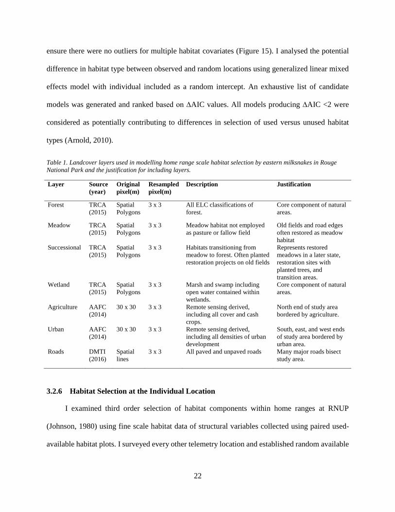
ensure there were no outliers for multiple habitat covariates (Figure 15). I analysed the potential

difference in habitat type between observed and random locations using generalized linear mixed

effects model with individual included as a random intercept. An exhaustive list of candidate

models was generated and ranked based on ∆AIC values. All models producing ∆AIC <2 were

considered as potentially contributing to differences in selection of used versus unused habitat

types (Arnold, 2010).

Table 1. Landcover layers used in modelling home range scale habitat selection by eastern milksnakes in Rouge

National Park and the justification for including layers.

Layer Source

(year)

Original

pixel(m)

Resampled

pixel(m)

Description Justification

Forest TRCA

(2015)

Spatial

Polygons

3 x 3 All ELC classifications of

forest.

Core component of natural

areas.

Meadow TRCA

(2015)

Spatial

Polygons

3 x 3 Meadow habitat not employed

as pasture or fallow field

Old fields and road edges

often restored as meadow

habitat

Successional TRCA

(2015)

Spatial

Polygons

3 x 3 Habitats transitioning from

meadow to forest. Often planted

restoration projects on old fields

Represents restored

meadows in a later state,

restoration sites with

planted trees, and

transition areas.

Wetland TRCA

(2015)

Spatial

Polygons

3 x 3 Marsh and swamp including

open water contained within

wetlands.

Core component of natural

areas.

Agriculture AAFC

(2014)

30 x 30 3 x 3 Remote sensing derived,

including all cover and cash

crops.

North end of study area

bordered by agriculture.

Urban AAFC

(2014)

30 x 30 3 x 3 Remote sensing derived,

including all densities of urban

development

South, east, and west ends

of study area bordered by

urban area.

Roads DMTI

(2016)

Spatial

lines

3 x 3 All paved and unpaved roads Many major roads bisect

study area.

3.2.6 Habitat Selection at the Individual Location

I examined third order selection of habitat components within home ranges at RNUP

(Johnson, 1980) using fine scale habitat data of structural variables collected using paired used-

available habitat plots. I surveyed every other telemetry location and established random available

23

locations within a distance accessible to the individual. (Row & Blouin-Demers, 2006c).

Beginning at the used location, we spun a compass to select a random bearing, then rolled a 20-

sided dice, multiplying the outcome by 10 to select a random number of steps to walk to a

theoretically available location (Row & Blouin-Demers, 2006c). Habitat plots were completed

when it was ensured through telemetry that the individual had moved to a new location (~2-14

days after collection of the occurrence record). I developed pair logistic regression models,

effective for comparing presence absence plots of wildlife, (Compton, Rhymer, & McCollough,

2002; Row & Blouin-Demers, 2006c) which considered a suite of biologically relevant variables,

both collected in the field and created post survey (Table 2).

Table 2. Names and definitions of variables used in modelling habitat selection at individual locations in Rouge

National Urban Park.

Name Definition

Vobstruct Height and density of surrounding vegetation: used a Robel pole to determine the visual minimum

and maximum height of vegetation and averaged these values

Dedge Distance to forest edge (> 10 clustered trees with adjoining canopy and DBH >10cm) to a maximum

of 15m

Canopy Percent canopy cover measured using a densitometer

Dcov Distance to nearest potential cover object (minimum 50cmx50cm)

Ncov Number of potential cover objects with 15 m of the location.

Sumcov The total area of cover objects available within 15m of the location. Derived area from length and

width measurements of individual objects and totaled their areas.

Vegheight The average vegetation height within a 1m radial plot of the exact location. Three measurements

were taken randomly and averaged.

DTree Distance to the nearest tree having a diameter at breast height >10cm, and occurring within 15m of

the location

I examined correlation between all predictors and evaluated those producing an unacceptable

level of correlation (r >0.6) with univariate models. Models were ranked based on ∆AIC and the

variables producing the lowest values were retained. All variables were scaled to center their

means on 0, and an exhaustive list of candidate models was generated. I ranked candidate models

based on ∆AIC values, considering those with ∆AIC <2 as potentially contributing to the

24

difference between presence and absence points (Arnold, 2010). Because variables were scaled,

lager coefficient values represented a larger effect on habitat selection.

3.3 Results

We collected 1001 observations of 30 individuals at QUBS over the 2003 and 2004 seasons,

and 453 locations of 17 individuals in RNUP throughout the 2015 and 2016 seasons (Table 3). I

compare these two datasets because QUBS has experienced little chance in vegetation structure

and habitat availability from data collection to present.

Table 3. Number of individual milksnakes tracked by site and sex, including metrics associated with the number of

relocation at Rouge National Urban Park and Queens University Biology Station.

Site Sex # of Individuals # of Relocations

Max Min Mean

RNUP M 12 39 6 23.58

F 5 42 18 31.6

QUBS M 20 51 9 30.75

F 10 52 14 36.3

3.3.1 Comparison of Home Range Sizes Between Sites

I excluded 5 individuals from RNUP due to their reproductive status and non-asymptotic

home range sizes, resulting in a total of 12 individuals (9 males, 3 females) for the analysis. At

QUBS, I excluded 8 individuals due to reproductive status and non-asymptotic home range,

leading to a total of 22 available individuals (19 males, 5 females).

Minimum convex polygons at the 95% level varied slightly between sites, with individual

home ranges at RNUP having both a smaller mean (RNUP=7.02±3.02ha, QUBS=11.84±3.26ha)

and reduced range (RNUP=1.54–23.38ha, QUBS=0.17ha–30.79) compared to the individuals at

QUBS (Figure 2). However, a multi-factor ANOVA found no significant difference in mean home

range size between sites (F=2.36, p=0.14). Difference in minimum convex polygon size is more

25

prevalent in males than females, with males also having larger average home range sizes at both

sites. However, a multi-factor ANOVA also found this to be non-significant (F = 0.56, p = 0.58).

A Tukey HSD test showed no significant difference within or between sexes across sites (all p-

values >0.70).

3.3.2 Differences in Movement Rates Between Sites

I derived DMRs for 30 individuals (19 males, 11 females) from QUBS and 17 individuals

(12 males, 5 females) from RNUP. Examining movement rates by sex, I found that males at RNUP

had smaller mean values than females while males at QUBS had larger mean values than females

(Figure 2). These differences between sexes were not statistically significant (DMR p = 0.64, DPM

p = 0.40). Examining differences between sites, I found that individuals at RNUP had larger DMR

(RNUP = 53.05 ± 14.83, QUBS = 29.26 ± 5.00) and distance per movement (RNUP = 64.56 ±

Figure 2. Box plots showing distance moved per day for individuals at Rouge National Urban Park

and Queens University Biology Station, and home range size of male and female milksnakes in each

study area.

26

15.61, QUBS = 47.54 ±20.22). The distance travelled per movement was significant (p = 0.18, t=

1.37, df = 48.58), while DMR was significantly higher (p = 0.01, t=2.69, df = 46.60) for

individuals at RNUP.

3.3.3 Road Avoidance in A Fragmented Landscape

Throughout the study no individuals crossed road, despite many locations being in close

proximity to different roads. The mean number of crossings per individual for simulated

movements was 3.4 ± 0.7 crossings and ranged from a low of 1.3 to a maximum of 5.1. A paired

t-test suggested that the random number of crossings was significantly higher than the number of

observed crossings (t=11.75, df=15, p= <0.001).

3.3.4 Habitat Selection at the Home Range Scale in Rouge National Urban Park

All 7 habitat covariates had an acceptable level of correlation (p<0.60). Using all covariates,

I developed an exhaustive list of models of which 7 contributed significantly to the difference

Figure 3. Standardized coefficients of top model and 97.5% confidence intervals potentially contributing to the

differences between used and available locations at the home range scale controlling for individual variation as a

random effect.

27

between used and absence locations (Table 4) Figure 15. Forest, meadow, urban, and agriculture,

appear in all top models and negatively influence occurrence to varying degrees (Figure 4).

Table 4. All candidate producing ∆AIC values <2 for milksnake habitat covariates at the home range scale

3.3.5 Habitat Selection at the Individual Location in Rouge National Urban Park

I found number of cover objects (Ncov) to have an unacceptable level of correlation with total

area of cover (Sumcov) (r=0.76) and distance to the nearest cover object (Dcov) (r=0.72), while

total area of cover (Sumcov) and distance to the nearest cover object (Dcov) showed an acceptable

level of correlation with each other (r=0.42). Distance to the nearest tree (Dtree) was also

correlated with canopy cover (Canopy) (r=0.61). Univariate models ranked based on ∆AIC

showed little difference between Distance to the nearest tree (Dtree) (∆AIC 0.00) and canopy cover

(Canopy) (∆AIC 1.48). I removed Distance to the nearest tree (Dtree), as prior knowledge on

milksnake habitat selection indicates that canopy cover and its associated thermal profile is a better

predictor of occurrence that tree cover (Row & Blouin-Demers, 2006b). Additional univariate

models examining the remaining 3 correlated variables led to the retention of number of cover

objects (Ncov) (∆AIC 0.00) rather than distance to the nearest cover object (Dcov) (∆AIC 4.98) or

total area of cover (Sumcov) (35.02). After removing correlated predictors, I used the 5 remaining

variables to develop an exhaustive series of 64 candidate models. I found that only the global

model produced a ∆AIC <2 (∆AIC=0.00). All models within ∆AIC <4 from the top model are

presented, as these are also thought to be competitive (Arnold, 2010), and assist in illustrating the

Model Formula ∆AIC

Occurrence∼Agriculture+Urban+Forest+Wetland+Road+Meadow 0

Occurrence∼Agriculture+Urban+Forest+Wetland+Road 0.059

Occurrence∼Agriculture+Urban+Forest+Wetland+Successional 0.272

Occurrence∼Agriculture+Urban+Forest+Wetland+Road+Successional 0.298

Occurrence∼Agriculture+Urban+Forest+Wetland 0.443

Occurrence∼Agriculture+Urban+Forest+Wetland+Meadow 1.083

Occurrence∼Agriculture+Urban+Forest+Wetland+Road+Meadow+Successional 1.993

28

importance of individual variables (Table 5). number of cover objects (Ncov) and canopy cover

(Canopy) appear in all 5 models producing a ∆AIC < 4.

Table 5. All candidate producing ∆AIC values <4, and potentially contributing to habitat selection by milksnakes at

the exact location.

Model Formula ∆AIC

Use ∼ Ncov+Canopy+Dedge+Vobstruct+Vegheight 0

Use ∼ Ncov+Canopy+Vobstruct+Vegheight 2.34

Use ∼ Ncov+Canopy+Dedge 2.66

Use ∼ Ncov+Canopy+Dedge+Vegheight 3.26

Use ∼ Ncov+Canopy+Dedge+Vobstruct 3.51

Examining the top model, all predictors were found to have 97.5% confidence intervals that did

not overlap with zero. The coefficients from the top model show a significant positive relationship

with number of cover objects (Ncov), distance to forest edge (Dedge), and visual obstruction

(Vobstruct) and a significant negative relationship with canopy cover (Canopy) and vegetation

height (Vegheight) (Figure 4).

Figure 4. Standardized coefficients of the top model and 97.5% confidence intervals contributing to the

difference between used and available locations.

29

3.4 Discussion

The results highlight the ecology of milksnakes in a developed region and point to potential

changes in movement rates and habitat selection patterns in disturbed areas. Along with these

changes, milksnakes avoid road crossings despite the close proximity of home ranges and

hibernacula to roads. At the home range scale, I found that individuals avoided urban areas, interior

forests, and agricultural fields. This was consistent with microhabitat selection where individuals

were shown to select for heterogeneous locations (higher surrounding structure, but low at-site

vegetation) with low canopy cover. Consistent with milksnakes in more natural areas, individuals

selected locations with a high numbers of potential cover objects.

There was no significant difference in home range size between sites, though home ranges at

RNUP had a large amount of overlap. These results are consistent with other studies that have

found no significant difference in snake home range sizes in response to varying degrees of

disturbance (Corey & Doody, 2010; Row et al., 2012). Though fragmentation often constrains

snake home range size (Vignoli, Mocaer, Luiselli, & Bologna, 2009), the non-territorial nature of

many snake species allows for overlap in home range providing sufficient resources are available

(Brattstrom, 1974). Increased home range overlap in fragmented regions been observed in other

snake species as a response to constraints on dispersal (Corey & Doody, 2010). The presence of a

road directly south of the main hibernaculum is likely constraining the directions which individuals

can disperse in RNUP, leading to increased overlap of home ranges relative to QUBS.

Movement rates in snakes are known to change seasonally (Shew, Greene, & Durbian, 2012),

vary between sexes, and are influenced by the availability of prey and thermal quality of habitat

(Brito, 2003; Friedlaender, 1982; King & Duvall, 1990; Madsen & Shine, 2006). Higher DMR at

RNUP cannot be accounted for by seasonal or between-sex variation, as movement rates were

analysed over the same duration, and the analysis included similar proportions of male and female

30

snakes at each site. The high amount of overlap between home ranges also points to the search for

mates not requiring extensive movement (Brito, 2003). When DMR has been considered in

response to anthropogenic influence, it has been found to be both significantly higher (Ettling et

al., 2016) and lower (Corey & Doody, 2010) in disturbed areas. However, Corey & Doody's (2010)

results are derived from a region where thermal quality is high at both sites and prey abundance is

higher at disturbed sites. Alternatively, Ettling et al (2016) found higher prey abundance at

disturbed versus natural sites. Low prey abundance in combination with high densities of predators

leads to competition for food sources in reptiles (Whitaker & Shine, 2002). Snakes are also known

to increase movement rates in response to decreased prey abundance (Mader, 1984; Madsen &

Shine, 2006). It is then possible that lower prey densities than QUBS and competition between

individuals within overlapping home ranges are leading to increased movement at RNUP.

Additionally, QUBS is more forested than RNUP and is known to be a thermally challenging

environment as snakes prioritize selection of thermal sites (Row & Blouin-Demers, 2006c). Snakes

movement is often constrained by the thermal quality of habitat, with lower movement rates

displayed as thermal quality decreases (D. S. Harvey & Weatherhead, 2010) . It is possible that

better thermal quality at RNUP then allows for increased movement. However, my data do not

include prey abundance or thermal quality of sites in RNUP.

Larger snake species are more likely to cross roads (Row et al., 2007) and their larger home

range sizes can necessitate crossings in urban areas (Bonnet, Naulleau, & Shine, 1999). Here, I

found milksnakes avoided road crossings based on a significantly higher number of crossings for

random movement paths than observed paths, which is consistent with some other snake species

in fragmented areas (Miller et al., 2017; Robson & Blouin-Demers, 2013; Siers, Savidge, & Reed,

2014). In fact, no milksnake in my study ever crossed a road. Milksnakes are a medium sized snake

31

and home range size did not appear to be constrained, suggesting habitat patch size combined with

milksnakes ecology did not necessitate crossings in RNUP. Perhaps if this study were to occur on

other sites with smaller patches of habitat, the degree of road avoidance may decrease.

Road avoidance may have long term genetic and population level consequences (Aresco, 2005;

Row et al., 2007; Shepard et al., 2008). Size of habitat patches can influence the persistence of

snake populations, and unwillingness to cross roads can dramatically decrease available patch size

in urban areas (Breininger et al., 2011; Goulet et al., 2015). Further, road avoidance can fragment

populations (Clark et al., 2010; Shepard et al., 2008) potentially increasing inbreeding effects (Row

et al., 2010). Although it appears that current habitat patches in RNUP are sufficiently large, there

are likely impacts of road avoidance on connectivity on a larger regional scale. Ecopassages have

been shown to improve genetic connectivity and decrease road mortality in snake species adjacent

to high traffic roads (Colley, Lougheed, Otterbein, & Litzgus, 2017). The establishment of

corridors connecting even moderate quality habitat can improve population connectivity (Row et

al., 2010, 2012), and may be important in improving the likelihood of persistence of milksnakes

across this region.

Although milksnakes are traditionally associated with some anthropogenic features (i.e. low

intensity farming), I found strong avoidance of urban areas at the home range scale. Agricultural

fields were not avoided suggesting a greater tolerance for this habitat, but the overall availability

of agricultural fields was low in the study area. Milksnakes also avoid interior forests which was

consistent with previous studies that have found milksnakes select forest edges and open habitats

(COSEWIC, 2002; Row & Blouin-Demers, 2006c). Interestingly, milksnakes seem to select early

successional habitat which made up a significant portion of the study area, and is largely comprised

of old fields that have undergone active restoration through wildlife seeding and tree planting.

32

Our analysis of third order habitat selection (Johnson, 1980) revealed that fine scale habitat

structure and heterogeneity of successional habitat likely plays a role in selection for this habitat

type. Individuals selected for higher overall vegetation density surrounding used locations, and

lower vegetation height at the exact location. This is potentially a trade-off between

thermoregulatory benefit and predation risk. Avian species are a significant predator of snakes

(Webb & Whiting, 2005) and the increased structure likely provides some visual obstruction.

Given that open habitats have greater thermal quality for milksnakes (Row & Blouin-Demers,

2006b) they are likely seeking out locations with greater sun exposure for basking (Charland P.T.

Gregory, 1995). In addition to the greater visual obstruction, milksnake choose locations with a

higher presence of cover objects which was consistent with natural sites and allows for retreat to

cooler sites for thermoregulation (Row & Blouin-Demers, 2006b), and for predator avoidance

(Charland P.T. Gregory, 1995). However, the type of cover objects varied between the sites with

primarily rock cover objects being replaced with foundations and anthropogenic debris at RNUP

(Row & Blouin-Demers, 2006c).

While I have found behavioural modifications, notably road avoidance, by milksnakes in

response to development, there is reason for optimism regarding the future of the Rouge Valley

population. The newly established Rouge National Urban Park (RNUP), a 78km2 reserve, largely

contains the known milksnake habitat and occurrence locations within the Rouge Valley and

represents a positive step towards conserving the species. Within RNUP, disturbance regimes that

maintain successional habitats should be promoted. Populations will also benefit from better

connection of these existing habitat patches across roads, potentially using ecopassages, to

facilitate movement. Furthermore, supplementing restored areas with artificial cover objects will

33

increase the availability of suitable microhabitats and likely assist milksnake populations long

term.

34

4 Assessing and Comparing Best Predicted Habitat of a Generalist and a

Specialist Snake Species Along an Urban Gradient

4.1 Introduction

Habitat loss and fragmentation are the largest global drivers of wildlife population declines

and contemporary extinctions (Brook, Sodhi, & Bradshaw, 2008; Fahrig, 1997). These impacts on

wildlife occur in all biomes due to human caused land use change driven by rapid human

population growth and urban development (Gallant, Klaver, Casper, & Lannoo, 2007; Hagen et

al., 2012). The most prevalent large-scale land use changes are clearing and conversion of natural

landscapes for agriculture or urban development (Gallant et al., 2007; Recio, Arija, Cabezas-Díaz,

& Virgós, 2015). Additionally, the associated transportation networks (e.g., roads) further divides

remaining habitat patches (Forman & Alexander, 1998) resulting in decreases in the amount of

habitat available on a landscape and the size of habitat patches, and increased patch isolation

(Fahrig, 2003). This creates a matrix of habitats divided by barriers that impedes the movement of

wildlife (Tucker et al., 2018).

Many native species and communities typically respond poorly to habitat fragmentation.

Species with large home ranges are often unable to access former home range areas following

human development and the animals are often subject to increased mortality rates or human

conflict in modified landscapes. (Congdon et al., 1994; Treves & Karanth, 2003). Specialized

species that are dependent on select habitat types or resources, and sessile species, may experience

the greatest impacts (Brouat, Chevallier, Meusnier, Noblecourt, & Rasplus, 2004; Devictor,

Julliard, & Jiguet, 2008). Additionally, species in fragmented habitats often avoid interaction with

humans, leading to isolation from suitable habitat patches (Lees & Peres, 2009). Even when

important habitat features are maintained they are functionally lost to the species if they are

unwilling or unable to traverse the matrix of unsuitable habitats (McKinney, 2006). Functional

35

habitat loss leads to genetic isolation between population clusters across multiple taxa (Fedy, Row,

& Oyler-McCance, 2017; Row et al., 2010). This can have long term population level effects,

increasing the likelihood of regional extinction or extirpation from habitat patches (Crooks et al.,

2017).

Generalist species are more capable of adapting to human modified landscapes, as they tend

to be mobile, have less specific habitat requirements or are able to modify behaviours, and have

high reproductive output (Devictor et al., 2008; Hagen et al., 2012). Impacts of development and

habitat fragmentation likely differ between specialist species. It is expected that specialist species

select fragmented habitats at larger scales than generalist species, and avoid small highly

fragmented patches. To understand which habitats are selected and the scales at which they are

selected by generalists and specialists in a fragmented region, comparisons should be made across

groups of related species. The Eastern Gartersnake (Thamnophis sirtalis sirtalis), a generalist, and

Eastern Milksnake (Lampropeltis triangulum), a specialist, are then excellent model species for

understanding responses to habitat fragmentation. They have significant range overlap, and are

both found in fragmented landscapes (COSEWIC, 2014; Kjoss & Litvaitis, 2001).

Both species use a combination of forest edges and open early successional habitats

(Charland P.T. Gregory, 1995; Row & Blouin-Demers, 2006c). Milksnakes are regarded as

specialists as they require microhabitats with high thermal quality and an abundance of cover

objects for basking (Row & Blouin-Demers, 2006c). Gartersnakes are considered generalists as

they bask indiscriminately in a variety of habitats (Charland & Gregory, 1995; Gibson & Falls,

1979). Milksnakes also have larger home ranges (5-10ha) than gartersnakes (~1.5ha)(Kjoss &

Litvaitis, 2001, Chapter 2), meaning some fragmented habitat patches may not be suitably large to

maintain milksnake populations. Additionally, snakes are known to avoid road crossings (Robson

36

& Blouin-Demers, 2013; Shepard et al., 2008, Chapter 3), making them ideal model species for

understanding the effects of habitat fragmentation.

To investigate the impact of habitat fragmentation between generalist and specialist species, I

focus on milksnake and gartersnake habitats in the heavily fragmented Greater Toronto Area

(herein GTA), which have significant range overlaps both historically and currently. I analysed

habitat selection across scales for both species at the landscape scale and investigate the strength

of selection and avoidance for multiple, biologically-relevant, landcover types. Using this

information, I mapped and compared best predicted multi-species habitat. I predicted that the

generalist, gartersnakes, would select smaller patches of a variety of natural landcover types, while

milksnakes were expected to select larger habitat patches. I predicted greater avoidance of human

modified landcover types in milksnakes than gartersnakes. Finally, I developed spatially-explicit

predictions of the relative probability of occupancy for each species and created an overlay of best

predicted habitat to understand the potential for multi-species conservation prioritization.

4.2 Methods

4.2.1 Study Area

The Greater Toronto Area is Canada’s largest metropolitan area with a population of

approximately 6 million (Conway & Hackworth, 2007; Vaz & Arsanjani, 2015). It is one of North

America’s fastest growing urban centers, and is expected to account for 80% of Ontario’s

population growth until 2030, putting it on track to become Canada’s first megacity (>10m

inhabitants) (Conway & Hackworth, 2007; Eidelman, 2010; Sahely, Dudding, & Kennedy, 2003;

Vaz & Arsanjani, 2015).

The natural areas in the core of Toronto are largely limited to the floodplains and ravines of

several rivers (Credit, Humber, Don, Rouge) and creeks that run generally north-south towards

37

Lake Ontario. The north end of the GTA includes parts of the Ontario Greenbelt, which places

formal protection on agricultural and natural lands through established limits on urban growth

(Eidelman, 2010). The largest natural areas in the region are to the north and represent secondary

growth forest along the Niagara Escarpment and Oak Ridges Moraine. Natural areas in the GTA

are highly fragmented by roads and developments (Figure 5). I delineated the study area within

the GTA based on the extent of the Toronto Region Conservation Authority (herein TRCA) and

Credit Valley Conservation Authority (herein CVC) management areas (Figure 5).

Figure 5. Map of the study area boundary is indicated by the black line. Snake survey locations (i.e., coverboards) are

indicated by the red circles. Study area boundary was defined by combining the Toronto Region Conservation Authority

and Credit Valley Conservation Authority boundaries. Major highways, cities, and natural areas (in green) can also be

seen in the background layer.

38

4.2.2 Occurrence and Absence Locations

Snake occurrence records were generated from 2015-2017 using a large scale coverboard

survey (Figure 5) as coverboards represent an effective low maintenance means of monitoring

herpetofauna (Grant et al., 1991). All boards were made of untreated plywood (dimensions 120cm

x 80cm x 2cm) and were placed between 2011 and 2015 based on historic snake occurrence

records, primarily incidental observations, obtained through the Natural Heritage Information

Centre (herein NHIC) (Figure 11, Figure 12). During checks, I visited all boards at a given site

recording environmental data (cloud cover, temperature, humidity), temperature under each board,

snake species present, morphometric measurements, and collected blood or tissue samples from

all snakes.

It is unlikely that contemporary snake populations have become established in areas with

no historic records, as snake dispersal is constrained by roads, development, and agricultural fields

(Lambeck, 1997; Mader, 1984). Due to the cryptic nature of milksnakes, I supplemented the

coverboard survey occurrence records with: (1) TRCA incidental occurrences, (2) CVC incidental

occurrences, and (3) road kill data collected by the Toronto Zoo (2011) in the Rouge Valley

watershed. Garter snake records were supplemented by CVC incidental occurrences. I created 1:1

pseudo-absence locations by randomly generating locations within landcover cells that did not

include occurrence points, and coded locations as 1 (occurrence) or 0 (pseudo-absence) (Barbet-

Massin, Jiguet, Albert, & Thuiller, 2012; Wisz & Guisan, 2009). All milksnakes were identified

by PIT tags or unique head markings, and repeat observations were not included as additional

occurrence locations.

39

4.2.3 Covariate Development

I developed a large-scale land cover map using remote sensing data obtained from

Agriculture & Agri-Foods Canada’s (herein AAFC) 2014 crop inventory (AAFC, 2014). Multiple

cover types were combined to create seven landcover layers prevalent within the study area Table

6). I derived six covariates from each landcover type including 3 density covariates and 3 decay

distance covariates for a total of 42 landcover covariates (Carpenter, Aldridge, & Boyce, 2010;

Nielsen, Cranston, & Stenhouse, 2009).

Table 6. Development of landcover layers used in the development of models and resource selection functions,

including landcover types used in building each layer (AAFC, 2014). Denotation by ǂ indicates a human-modified

landcover type.

Density covariates were generated using 3 moving windowMW sizes (250mMW250, 500mMW500,

1000mMW1000) for each landcover type. Multiple scales were chosen to represent the highly

Landcover

Type

Inputs from

AAFC Data

Description Justification

Forest

30m x 30m

Broadleaf forest

Mixed wood forest

Coniferous forest

Undifferentiated

Forest

All predominantly trees

landscapes.

Forest edges important for

thermoregulation (Row & Blouin-

Demers, 2006c).

Successional

30m x 30m

Shrubland Woody vegetation, +/-2m in

height.

Influential in home range-scale habitat

selection (Chapter 2).

Wetland

30m x 30m

Wetland Semi-permanent and permanent

wetland vegetation, omitting open

water.

Natural area network contains

floodplains and wetland areas

unsuitable for development

Grassland

30m x 30m

Grassland Native grasses and herbaceous

vegetation.

Commonly used for basking by snakes

(Ralph Gibson & Bruce Falls, 1979).

Field ǂ

30m x 30m

Fallow field

Pasture

Non-permanent grasslands subject

to seasonal and annual changes,

typically non-native species.

Common in marginal agricultural

lands.

Historic association with milksnake

occurrence (COSEWIC, 2014)

Agriculture ǂ

30m x 30m

Cereal crops

Legumes

Vegetables

Fruits

Several combined crops,

representing all agricultural land

use.

Negative association with snake

occurrence (COSEWIC, 2014)

Urban ǂ

30m x 30m

Urban All roads, railways, paved

surfaces, urban residential,

commercial, industrial, other

buildings.

Negative association with snake

occurrence (Chapter 2)

40

variable size and layout of natural areas in the study area, and scale dependent habitat selection

processes in snakes (Chapter 2, Row & Blouin-Demers, 2006). Decay distanceDD variables were

created using an exponential decay function e-a/d where a was set at 250mDD250, 500mDD500, and

1000mDD1000, d was the distance from a given cell to the given landcover type. Decay distances

was chosen rather than linear distance due to species inherently non-linear responses to habitat,

and due to known impacts of anthropogenic landcover on snake behaviour and populations (Corey

& Doody, 2010; Ettling et al., 2016).

4.2.4 Model Development and Selection

I next determined which of the 6 covariates within each landcover type were the best predictors

of occurrence for each species. Each covariate was assessed in a univariate generalized linear

model (GLM) with a binomial link function used for presence-absence data. GLMs were chosen

as they are ideal for use with presence/pseudo-absence data (Chefaoui & Lobo, 2008; Tsoar,

Allouche, Steinitz, Rotem, & Kadmon, 2007). Each univariate model also included an intercept-

only model for comparison. When the intercept-only model outperformed the univariate model,

the variable was dropped from further consideration. Univariate models were ranked based on their

∆AIC values, and the model producing the lowest value was considered the top covariate for the

given landcover type and species. This process produced a list of 7 unique landcover covariates

representing the seven landcover types for each species.

I examined correlation between the 7 landcover covariates to ensure no pairs produced an

unacceptable level of correlation (Pearson’s r ≥ |0.65|) to avoid issues of multicollinearity. Using

the top covariate for each landscape layer, I developed global models for both species using GLMs

with a binomial link function to predict the probability of occurrence. I considered all possible

model combinations for each species, ranked models based on AIC values, and selected the top

41

model (producing the lowest ∆AIC). All models within ∆AIC <2 were considered as potentially

contributing to differences between occurrence and absence locations (Arnold, 2010). I examined

top model covariates and inferred relationships between human disturbance and likelihood of

occurrence from all top models. The top model was predicted spatially as a resource selection

function (RSF) with a continuous 0-1 scale representing predicted probability of occurrence.

4.2.5 Model Evaluation and Comparison

I evaluated the performance of each RSF using the Boyce validation index (i.e. k-fold cross

validation) (Boyce, Vernier, Nielsen, & Schmiegelow, 2002). Spearman-rank correlation was

calculated between bins, and model performance was assessed based on the average Spearman-

rank correlation across all bins (Boyce et al., 2002). High correlation values between bins suggests

a model that preforms well in predicting likelihood of occurrence (Boyce et al., 2002).

To directly compare species, I used the landcover covariates from the top model from each

species to model the other species, and compared the coefficients. To identify areas with the best

predicted habitat for both species, I created an map summing the two RSF’s. I considered all values

above the third quartile of the probability distribution (i.e. top 25% of all pixels) for each RSF to

constitute good habitat (Fedy, Devries, Howerter, & Row, 2018). These values were transformed

to 1, and all values below the third quartile were coded as 0. The remaining values for both species

were summed to produce a surface showing areas with best predicted habitat for 2, 1, or neither

species.

42

4.3 Results

I placed 385 boards at 53 sites during the 2015 season and combined with the 88 boards placed

at 2 sites by the Toronto Zoo in 2011, the coverboard survey included 473 boards at 54 sites. This

generated 78 milksnake records and 82 gartersnake records through the coverboard survey, and

supplemented these with an additional 114 milksnake records and 175 gartersnake records (Table

7).

Table 7. Summary of occurrence used in modelling and to develop resource selection functions.

Species Coverboards Roadkill Surveys CVC TRCA Total

Milksnake 78 18 55 41 192

Gartersnake 82 0 58 117 257

4.3.1 Model Selection

None of the covariates were unacceptably correlated (r < 0.6). Univariate model comparisons

consistently resulted in milksnakes responding (both positively and negatively) to habitat types at

larger scales. Differing scale of responses to habitat types is most apparent in agriculture, forest,

wetland, and grassland where milksnake univariate models preformed best at 1000m while

gartersnakes did so at 250m.

All possible model combinations were compared (n = 128) for each species. Seven milksnake

models and 3 gartersnake models were within ∆AIC <2 and were considered the top models. Of

the top milksnake models, all contained covariates representing agriculture MW1000, forest MW1000,

and wetland MW1000 (Table 8) The top model consisted of only these 3 covariates, while 5 of 6 other

top models were a combination of this model plus one additional covariates (Table 8) Of the top 3

gartersnake models, all contained agriculture MW250, forest DD250, wetland DD1000, field MW500 and

urban MW250, while the top model also contained grassland DD1000 (Table 8). Coefficient estimates

were consistently negative or positive across the top models.

43

Table 8.Milksnake and gartersnake model tables including all candidate producing ∆AIC values <2, and potentially

contributing to occurrence locations.

The top models for both species contained positive coefficient estimates for forest and

wetland and negative estimates for agriculture (Figure 6, Figure 7). None of the coefficients in the

top models had 85% confidence interval that overlapped zero (Figure 6, Figure 7). Milksnakes

showed less consistent negative association with human modified landcover types urban (2

models) and agriculture (all competitive models) across all competitive models. However, urban

did produce negative coefficient estimates in these two competitive milksnake models. Effects plot

demonstrate similar negative responses to urban and agriculture, while responses to field vary

between species (Figure 8).

4.3.2 Resource Selection Functions

Both RSF’s had high Spearman correlation between bins for occurrence locations and

therefore strong predictive capacity (EMS mean correlation = 0.98, EGS mean correlation = 0.92).

4.3.3 Species Comparisons

Comparing the top milksnake model between species, it is clear that milksnakes select for or

select against fewer landcover types at larger spatial scales. Applying gartersnake date to the 3

Milksnake Model Formulas ∆AIC

Occurrence~AgricultureMW1000+ForestMW1000+WetlandMW1000 0

Occurrence~AgricultureMW1000+ForestMW1000+WetlandMW1000+SuccessionalDD1000 0.12

Occurrence~AgricultureMW1000+ForestMW1000+WetlandMW1000+UrbanMW250 0.64

Occurrence~AgricultureMW1000+ForestMW1000+WetlandMW1000+FieldDD250 1.49

Occurrence~AgricultureMW1000+ForestMW1000+WetlandMW1000+SuccessionalDD1000+Field

DD250 1.57

Occurrence~AgricultureMW1000+ForestMW1000+WetlandMW1000+SuccessionalDD1000+Urban

MW250 1.89

Occurrence~AgricultureMW1000+ForestMW1000+WetlandMW1000+GrasslandDD1000 1.99

Gartersnake Model Formulas ∆AIC

Occurrence~AgricultureMW250+ForestDD250+FieldMW1000+UrbanMW250+WetlandDD1000Gr

asslandMW500 0

Occurrence~AgricultureMW250+Forest DD250+FieldMW500+UrbanMW250+Wetland DD1000 1.30

Occurrence~AgricultureMW250+ForestDD250+FieldMW500+UrbanMW250+WetlandDD1000+G

rasslandMW500+SuccessionalDD1000 1.78

44

landcover covariates from the milksnake, it is clear that selection and avoidance at these scales is

stronger in milksnakes. Best predicted habitat for both species is primarily available through the

Greenbelt areas north of the study area and the Rouge Valley to east of the study area. Relatively

continuous habitat is available through these areas, while all locations through the core of the GTA

have isolated patches of best predicted habitat (Figure 9). Comparing this map to the RSFs, it is

apparent that best predicted habitat for both species is constrained by the availability of highly

suitable milksnake habitat (Figure 10).

45

Figure 6. Coefficient estimates from gartersnake top model. Coefficients for milksnakes, produced using the landcover

covariates from the gartersnake top model, are also displayed.

46

Figure 7. Coefficient estimates from milksnake top model. Coefficients for gartersnakes, produced using the

landcover covariates from the milksnake top model, are also displayed.

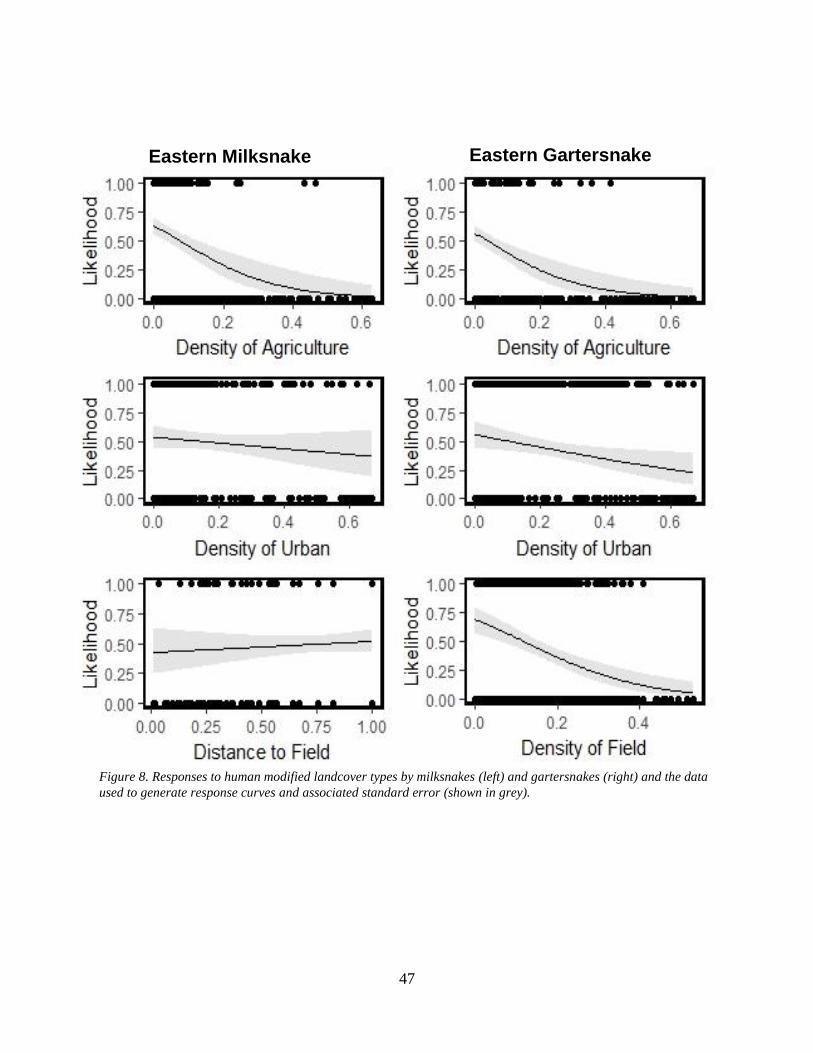
47

Eastern Gartersnake Eastern Milksnake

Figure 8. Responses to human modified landcover types by milksnakes (left) and gartersnakes (right) and the data

used to generate response curves and associated standard error (shown in grey).

48

Figure 9. Resource selection functions for eastern milksnake and eastern gartersnake including all occurrence

locations (black) used in model development and coverboard locations (red) used to gather occurrence records.

Scale bars represent increasing relative probability of occurrence.

49

Figure 10. Areas with high likelihood of occurrence for gartersnake and milksnake (blue), or one of these species (red) within the

study area. Areas with low likelihood of occurrence for both species are not highlighted.

50

4.4 Discussion

The generalist and specialist species focused on in this research demonstrated differential

patterns of habitat use consistent with their life history strategies across a highly fragmented

region. The top model set for the specialist species, milksnakes, contained a greater number of

models having generally fewer variables than the generalist species, gartersnakes. The suite of top

milksnake models had consistently positive coefficient estimates for forest and wetland cover

which were also present, though at smaller scales, in the top gartersnake models which also all

demonstrated negative associations with fallow fields and pastures (field). Both species avoided

human-modified landscapes represented by agriculture cover, and the top gartersnake models also

indicated avoidance of urban areas. There is also a notable difference in the scale at which each

species responds to landcover types, as milksnakes consistency responded to habitat types at larger

scales. This is evident in the maps of predicted likelihood of occurrence as smaller patches of

natural area surrounded by human modified landscapes are not suitable for milksnakes, leading to

best predicted multi-species habitat being constrained by milksnake occurrence.

The competitive model sets indicate that the milksnakes have more specific habitat

requirements as they contain fewer variables. This is consistent with my prediction, and other

literature demonstrating that habitat selection models for specialist snake species result in a

stronger response to fewer natural landcover types than generalist species in the same region

(Segura, Feriche, Pleguezuelos, & Santos, 2007). Previous research has demonstrated that

milksnakes use forest edge habitats for thermoregulation, and this is supported in the landscape-

scale study in the positive association with forest cover (Row & Blouin-Demers, 2006c). Snake

species in forested landscapes also make use of small open habitat patches (Kjoss & Litvaitis,

2001) created by micro disturbances as small as single treefall events (Canham et al., 1990), which

51

would be difficult to detect at the spatial resolution of the data. Resolution may also explain why

successional habitat is important at the micro-habitat and home range scales for milksnakes

(Chapter 2), but does not influence likelihood of occurrence at the landscape scale.

Surprisingly, the avoidance of urban areas was more prevalent in the top models for

gartersnakes than milksnakes, contrary to my prediction that milksnakes would demonstrate

greater avoidance than gartersnakes. The negative association with agriculture by gartersnakes and

scale of the response (250m) suggests that gartersnakes use habitats directly bordering agriculture.

Gartersnakes are known as dietary generalists (Kephart & Arnold, 1982), and generalist snake

species can modify behaviours to use crop monocultures and intensive agricultural areas when

prey is abundant in these areas (Ettling et al., 2016; Wisler, Hofer, & Arlettaz, 2008). While the

results show avoidance of agriculture, the scale of the response and species biology suggest they

may occasionally use these areas. The slight positive response in milksnakes to increased distances

from fieldDD250, compared to gartersnakes strong negative response to density of fieldMW1000 can

be attributed to species life history. Milksnakes are historically associated with low intensity

agriculture and make frequent use of human structures (i.e. barns, buildings) in these landscapes

(COSEWIC, 2014; Lentini et al., 2015; Row & Blouin-Demers, 2006c). Agricultural fields taken

out of production and low intensity agriculture have been noted to benefit other specialist snake

species (Kjoss & Litvaitis, 2001; R Shine & Fitzgerald, 2006). However, this habitat type occurs

infrequently in the study area as low intensity agricultural areas are in decline, in favour of larger

scale farming (Gallant et al., 2007) The negative association with urban areas is also consistent

between species. However, the data do not include between type (i.e. detached homes, high rises)

or age of urban development, which is influences natural area patch size and herpetofauna

occupancy (Vignoli et al., 2009).

52

Milksnakes consistently responded to landcover types at larger scales than gartersnakes as

they are more sensitive to disturbance and require larger tracts of suitable habitat. The conservation

of coastal and riparian wetlands is a priority at the landscape scale within in the study area (Croft-

White, Cvetkovic, Rokitnicki-Wojcik, Midwood, & Grabas, 2017). The conservation of these

areas and relative lack of human disturbance likely influences the strong positive associations for

both species to wetland habitat types at the same scale (MW1000, DD1000). Milksnakes are also

selecting forest habitat (MW1000) and avoiding agriculture (MW1000) and urban (MW1000) habitat at

much larger scales than gartersnakes (DD250, MW250, MW250). This is evident in the spatially precited

RSF`s, as suitable gartersnake habitat can often follow small corridors of natural habitat adjacent

to urban areas, whereas these habitats are normally considered to be unsuitable for milksnakes.

Minimum area requirements for specialist species are often not met in areas of intensive

development (Vignoli et al., 2009) and these impacts are compounded because milksnake home

ranges are much larger than gartersnakes (Kjoss & Litvaitis, 2001, Chapter 2).

Suitable habitat patches large enough for milksnakes likely do not exist in direct proximity to

urban and agricultural areas in the study region. The best predicted multi-species habitat is then

limited by milksnakes, meaning prioritization of milksnake habitat would also adequately conserve

gartersnake habitat. These findings offer some support for the use of focal species in conservation

prioritisation where species have known range overlap (Bifolchi & Lodé, 2005; Roberge &

Angelstam, 2004). While this approach would neglect small patches of suitable gartersnake

habitat, these patches are comprised of parkland and riparian areas that are not under further

development pressure. The best predicted multi species habitats found in the study area occur in

larger natural areas and along an ex-urban gradient. Large, well-connected, natural areas are

consistently shown to benefit specialist species in fragmented landscapes (Lees & Peres, 2009;

53

Tischendorf, Bender, & Fahrig, 2003) and this appears to be the case for milksnakes in this study.

However, these ex-urban areas are facing increasing development pressure (Gallant et al., 2007;

Recio et al., 2015). Without effort to protect ex-urban areas including low-intensity agriculture

and large tracts of forest and wetland habitats, intensive agriculture and development will likely

have long term negative effects on milksnake and gartersnake populations.

Milksnakes, a specialist species, are selecting fewer habitat types as being suitable at larger

scales than gartersnakes, a generalist species. As predicted, high quality multi-species habitat is

driven by the distribution of milksnakes which typically contains habitats also suitable to

gartersnakes. In order to effectively conserve both species, conservation of the remaining larger

natural areas along an ex-urban gradient should be prioritized. In the context of the GTA, this

should focus on preserving existing habitat along the north end of the Credit Valley and Toronto

Region Conservation Authority management areas, and northeast end of the study area which is

currently facing development pressures.

54

5 Conclusions

This study quantifies milksnake habitat selection and behavioural adaptation in response to

human development. My results indicate changes in movement rates and habitat selection patterns

in disturbed areas, potentially due to constraints by roads and an unwillingness to make crossings.

Though the study area is highly fragmented, these findings come from relatively large patches. In

order to fully understand the impact of roads, future research should estimate population size and

genetic distribution to understand source-sink dynamics of individual habitat patches. Milksnakes

avoid urban areas, interior forests, and agricultural fields at the home range scale, while selecting

for successional habitat. Microhabitat selection favors heterogeneous locations near forest edges

(higher surrounding structure, but low at-site vegetation) with low canopy cover, and abundant

cover, likely owing to a trade-off between thermoregulatory benefit and predator avoidance.

Selection for open habitats and abundant cover is consistent with what is known to occur in natural

landscapes

At the landscape scale, milksnakes (a specialist species) and gartersnakes (a generalist species)

were found to have differential patterns of habitat selection both in terms of habitat type and the

scale at which selection is occurring. Both species appear to be selecting for forest and wetland

habitat, and avoiding urban and agricultural areas. This response is occurring at different scales,

with milksnakes consistently responding at larger scales which indicates increased avoidance of

human modified landscapes and a preference for large natural areas. Gartersnakes occur

throughout highly fragmented landscapes, as they are able to use small habitat patches unsuitable

for milksnakes. High quality multi species habitat is then limited by the distribution of milksnakes,

and occurs primarily in the northern end of the TRCA and CVC management areas, and the

northeast end of the study area.

55

Overall, I recommend the restoration of marginal agricultural areas surrounding existing

natural corridors to meadow and successional habitat to allow for movement between patches.

Selection for forest and wetland at the landscape scale means that priority should also be put on

expanding or maintaining large natural areas, which would effectively conserve habitat for both

milksnakes and gartersnakes. This would also create an abundance of edge habitat, and would

allow current forests to age and create micro-disturbances which lead to suitable microhabitats. It

should also be notes that areas selected as parts of natural corridors should contain milksnake

populations, as the number of roads in the study area limits dispersal to suitable habitat patches. If

populations do not exist, efforts should be made, potentially through the use of underpasses, to

connect suitable habitats. This requires future research to estimate population sizes in different

habitat patches, and assess genetic connectivity of populations, in order to understand patch

source/sink dynamics. The presence of RNUP in the study area creates a potential refuge for

milksnake populations. However, natural corridors containing a diversity of microhabitats and

other large natural areas should be established to ensure long term persistence of milksnakes in the

Greater Toronto Area.

56

6 References

AAFC. (2014). AAFC Crop Type Feature Catalog.

Aebischer, N. J., Robertson, P. A., & Kenward, R. E. (1993). Composition analysis of habitat use

from animal radio-tracking data. Ecology, 74(5), 1313–1325.

http://doi.org/10.2307/1940062

Aresco, M. J. (2005). The effect of sex-specific terrestrial movements and roads on the sex ratio

of freshwater turtles. Biological Conservation, 123(1), 37–44.

http://doi.org/10.1016/j.biocon.2004.10.006

Arnold, T. W. (2010). Uninformative Parameters and Model Selection Using Akaike’s

Information Criterion. Journal of Wildlife Management, 74(6), 1175–1178.

http://doi.org/10.2193/2009-367

Atwood, T. C. (2006). The influence of habitat patch attributes on coyote group size and

interaction in a fragmented landscape. Canadian Journal of Zoology, 84(1), 80–87.

http://doi.org/10.1139/z05-180

Barbet-Massin, M., Jiguet, F., Albert, C. H., & Thuiller, W. (2012). Selecting pseudo-absences

for species distribution models: how, where and how many? Methods in Ecology and

Evolution, 3(2), 327–338. http://doi.org/10.1111/j.2041-210X.2011.00172.x

Bender, D. J., Contreras, T. A., & Fahrig, L. (1998). Habitat Loss and Population Decline : A

Meta-Analysis of the Patch Size Effect Author, 79(2), 517–533.

Bifolchi, A., & Lodé, T. (2005). Efficiency of conservation shortcuts: An investigation with

otters as umbrella species. Biological Conservation, 126(4), 523–527.

http://doi.org/10.1016/j.biocon.2005.07.002

Bonnet, X., Naulleau, G., & Shine, R. (1999). The dangers of leaving home: Dispersal and

mortality in snakes. Biological Conservation, 89(1), 39–50. http://doi.org/10.1016/S0006-

3207(98)00140-2

Boyce, M. S., Vernier, P. R., Nielsen, S. E., & Schmiegelow, F. K. A. (2002). Evaluating

resource selection functions. Ecological Modelling, 157(2–3), 281–300.

http://doi.org/10.1016/S0304-3800(02)00200-4

Boyle, S. A., Lourenço, W. C., Da Silva, L. R., & Smith, A. T. (2009). Home range estimates

vary with sample size and methods. Folia Primatologica, 80(1), 33–42.

http://doi.org/10.1159/000201092

Brattstrom, B. H. (1974). The evolution of reptilian social behavior. Integrative and

Comparative Biology, 14(1), 35–49. http://doi.org/10.1093/icb/14.1.35

Breininger, D. R., Bolt, M. R., Legare, M. L., Drese, J. H., Stolen, E. D., Reininger, D. A. R. B.,

… Rese, J. O. H. N. H. D. (2011). Factors Influencing Home-Range Sizes of Eastern Indigo

Snakes in Central Florida Published By : The Society for the Study of Amphibians and

Reptiles Factors Influencing Home-Range Sizes of Eastern Indigo Snakes in Central

Florida, 45(4), 484–490.

57

Brito, J. C. (2003). Seasonal Variation in Movements , Home Range , and Habitat Use by Male

Vipera latastei in Northern Portugal, 37(1), 155–160.

Brook, B. W., Sodhi, N. S., & Bradshaw, C. J. A. (2008). Synergies among extinction drivers

under global change. Trends in Ecology and Evolution, 23(8), 453–460.

http://doi.org/10.1016/j.tree.2008.03.011

Brouat, C., Chevallier, H., Meusnier, S., Noblecourt, T., & Rasplus, J. Y. (2004). Specialization

and habitat: Spatial and environmental effects on abundance and genetic diversity of forest

generalist and specialist Carabus species. Molecular Ecology, 13(7), 1815–1826.

http://doi.org/10.1111/j.1365-294X.2004.02206.x

Buskirk, S. W., & Millspaugh, J. J. (2006). Metrics for Studies of Resource Selection. Journal of

Wildlife Management, 70(2), 358–366. http://doi.org/10.2193/0022-

541X(2006)70[358:MFSORS]2.0.CO;2

Byer, N. W., Smith, S. A., & Seigel, R. A. (2017). Effects of Site, Year, and Estimator Choice on

Home Ranges of Bog Turtles ( Glyptemys muhlenbergii) in Maryland. Journal of

Herpetology, 51(1), 68–72. http://doi.org/10.1670/15-150

Cagnolo, L., Valladares, G., Salvo, A., Cabido, M., & Zak, M. (2009). Habitat fragmentation and

species loss across three interacting trophic levels: Effects of life-history and food-web

traits. Conservation Biology, 23(5), 1167–1175. http://doi.org/10.1111/j.1523-

1739.2009.01214.x

Calenge, C. (2006). The package “adehabitat” for the R software: A tool for the analysis of space

and habitat use by animals. Ecological Modelling, 197(3–4), 516–519.

http://doi.org/10.1016/j.ecolmodel.2006.03.017

Canham, C. D., Denslow, J. S., Platt, W. J., Runkle, J. R., Pries, T. A., & White, P. S. (1990).

Light regimed beneath closed camopies and tree-fall gaps in temperate and tropical forests.

Canadian Journal of Forest Research, 20(5), 620–631.

http://doi.org/https://doi.org/10.1139/cjfr-2016-0466

Carpenter, J., Aldridge, C., & Boyce, M. S. (2010). Sage-Grouse Habitat Selection During

Winter in Alberta. Journal of Wildlife Management, 74(8), 1806–1814.

http://doi.org/10.2193/2009-368

Charland P.T. Gregory, M. B. (1995). Movements and habitat use in gravid and nongravid femal

garter snakes (Colubridae: Thamnophis). J. Zool., London, 236, 543–561.

Chefaoui, R. M., & Lobo, J. M. (2008). Assessing the effects of pseudo-absences on predictive

distribution model performance. Ecological Modelling, 210(4), 478–486.

http://doi.org/10.1016/j.ecolmodel.2007.08.010

Clark, R. W., Brown, W. S., Stechert, R., & Zamudio, K. R. (2010). Roads, interrupted dispersal,

and genetic diversity in timber rattlesnakes. Conservation Biology, 24(4), 1059–1069.

http://doi.org/10.1111/j.1523-1739.2009.01439.x

Colley, M., Lougheed, S. C., Otterbein, K., & Litzgus, J. D. (2017). Mitigation reduces road

mortality of a threatened rattlesnake. Wildlife Research, 44(1), 48–59.

http://doi.org/10.1071/WR16130

58

Compton, B. W., Rhymer, J. M., & McCollough, M. (2002). Habitat selection by wood turtles

(Clemmys insculpta): An application of paired logistic regression. Ecology, 83(3), 833–843.

http://doi.org/10.1890/0012-9658(2002)083[0833:HSBWTC]2.0.CO;2

Congdon, J. D., Dunham, A. E., & van Loben Sels, R. C. (1994). Demographics of Common

Snapping Turtles ( Chelydra Serpentina ): Implications for Conservation and Management

of Long-Lived Organisms Author ( s ): Justin D . Congdon , Arthur E . Dunham , R . C .

van Loben Sels Published by : Oxford University Press Stab. American Zoologist, 34(3),

397–408.

Conway, T., & Hackworth, J. (2007). Urban pattern and land cover variation in the greater

Toronto area. Canadian Geographer, 51(1), 43–57. http://doi.org/10.1111/j.1541-

0064.2007.00164.x

Corey, B., & Doody, J. S. (2010). Anthropogenic influences on the spatial ecology of a semi-arid

python. Journal of Zoology, 281(4), 293–302. http://doi.org/10.1111/j.1469-

7998.2010.00705.x

COSEWIC. (2014). Assessment and Status Report: Eastern Milksnake.

Croft-White, M. V., Cvetkovic, M., Rokitnicki-Wojcik, D., Midwood, J. D., & Grabas, G. P.

(2017). A shoreline divided: Twelve-year water quality and land cover trends in Lake

Ontario coastal wetlands. Journal of Great Lakes Research, 43(6), 1005–1015.

http://doi.org/10.1016/j.jglr.2017.08.003

Crooks, K. R., Burdett, C. L., Theobald, D. M., King, S. R. B., Di Marco, M., Rondinini, C., &

Boitani, L. (2017). Quantification of habitat fragmentation reveals extinction risk in

terrestrial mammals. Proceedings of the National Academy of Sciences, 114(29), 7635–

7640. http://doi.org/10.1073/pnas.1705769114

Davis, A. M., & Glick, T. F. (1978). Urban Ecosystems and Island Biogeography. Environmental

Conservation, 5(4), 299. http://doi.org/10.1017/S037689290000638X

Deelstra, T. (1988). Towards Ecological Sustainable Cities: Strategies, Models, and Tools In

Urban Ecology. (H. Feldmann & O. Uhlmann, Eds.). Berlin.

Devictor, V., Julliard, R., & Jiguet, F. (2008). Distribution of specialist and generalist species

along spatial gradients of habitat disturbance and fragmentation. Oikos, 117(4), 507–514.

http://doi.org/10.1111/j.0030-1299.2008.16215.x

Diffendorfer, J. E., Rochester, C., Fisher, R. N., & Brown, T. K. (2005). Movement and Space

Use by Coastal Rosy Boas (Lichanura trivirgata roseofusca) in Coastal Southern California.

Journal of Herpetology, 39(1), 24–36. http://doi.org/10.1670/212-03A

Eidelman, G. (2010). Managing Urban Sprawl in Ontario. Politics & Policy, 38(6), 1211–1236.

http://doi.org/10.1111/j.1747-1346.2010.00275.x

Elith, J., & Leathwick, J. R. (2009). Species Distribution Models: Ecological Explanation and

Prediction Across Space and Time. Annual Review of Ecology, Evolution, and Systematics,

40(1), 677–697. http://doi.org/10.1146/annurev.ecolsys.110308.120159

Elton, C. (1927). Animal Ecology.

59

Ettling, J. A., Aghasyan, L. A., Aghasyan, A. L., & Parker, P. G. (2016). Spatial Ecology of

Armenian Vipers, Montivipera raddei , in Two Different Landscapes: Human-Modified vs.

Recovered-Natural. Russian Journal of Herpetology, 23(2), 93–102.

http://doi.org/10.1643/CE-11-172

Ewers, R. M., & Didham, R. K. (2006). Confounding factors in the detection of species

responses to habitat fragmentation. Biological Reviews of the Cambridge Philosophical

Society, 81(1), 117–142. http://doi.org/10.1017/S1464793105006949

Faaborg, J., Brittingham, M., Donovan, T., & Blake, J. (1993). Habitat fragmentation in the

temperate zone: a perspective for managers. Retrieved from

http://www.treesearch.fs.fed.us/pubs/22917

Fahrig, L. (1997). Relative Effects of Habitat Loss and Fragmentation on Population Extinction.

Journal of Wildlife Management, 61(3), 603–610.

Fahrig, L. (2003). Effects of Habitat Fragmentation on Biodiversity. Annual Review of Ecology,

Evolution, and Systematics, 34(1), 487–515.

http://doi.org/10.1146/annurev.ecolsys.34.011802.132419

Fedy, B. C., Devries, J. H., Howerter, D. W., & Row, J. R. (2018). Distribution of priority

grassland bird habitats in the Prairie Pothole Region of Canada, 13(1).

http://doi.org/10.5751/ACE-01143-130104

Fedy, B. C., Row, J. R., & Oyler-McCance, S. J. (2017). Integration of genetic and demographic

data to assess population risk in a continuously distributed species. Conservation Genetics,

18(1), 89–104. http://doi.org/10.1007/s10592-016-0885-7

Forman, R. T. T., & Alexander, L. E. (1998). Roads and Their Major Ecological Effects. Annual

Review of Ecology and Systematics, 29(1), 207–231.

http://doi.org/10.1146/annurev.ecolsys.29.1.207

Friedlaender, J. B. (1982). Society for the Study of Amphibians and Reptiles Movements and

Temperature Relationships of Timber Rattlesnakes ( Crotalus horridus ) in Northeastern

New York Author ( s ): William S . Brown , Donald W . Pyle , Kimberly R . Greene and

Jeffrey B . Friedlae. Journal of Herpetology, 16(2), 151–161.

Gallant, A. L., Klaver, R. W., Casper, G. S., & Lannoo, M. J. (2007). Global rates of habitat loss

and implications for amphibian conservation. Copeia, 2007(4), 967–979.

http://doi.org/10.1643/0045-8511(2007)7[967:GROHLA]2.0.CO;2

Germaine, S. S., & Wakeling, B. F. (2001). Lizard species distributions and habitat ocupation

along an urban gradient in Tucson, Arizona, USA. Biological Conservation, 97, 229–237.

Gibbons, W. J., Scott, D. E., Ryan, T. J., Buhlmann, K. A., Tuberville, T. D., Metts, B. S., …

Winne, C. T. (2000). The Global Decline of Reptiles , Déjà Vu Amphibians. BioScience,

50(8), 653–666. http://doi.org/10.1641/0006-3568(2000)050[0653:TGDORD]2.0.C

Gill, J. A., Sutherland, W. J., & Watkinson, A. R. (1996). A Method to Quantify the Effects of

Human Disturbance on Animal Populations Author, 33(4), 786–792.

Goulet, C., Litvaitis, J. A., & Marchand, M. N. (2015). Habitat Associations of the Eastern

60

Hognose Snake at the Northern Edge of Its Geographic Distribution: Should a Remnant

Population Guide Restoration? Northeastern Naturalist, 22(3), 530–540.

http://doi.org/10.1656/045.022.0309

Grant, B. W., Tucker, A. D., Lovich, J. E., Mills, A. M., Dixon, P. M., & Gibbons, J. W. (1991).

The use of coverboards in estimating patterns of reptile and amphibians biodiversity.

Wildlife 2001: Populations. http://doi.org/10.1007/978-94-011-2868-1

Grinnell, 1917. (n.d.).

Guisan, a, & Zimmermann, N. E. (2000). Predictive habitat distribution models in ecology.

Ecological Modelling, 135, 147–186. http://doi.org/10.1016/S0304-3800(00)00354-9

Hagen, M., Kissling, W. D., Rasmussen, C., De Aguiar, M. A. M., Brown, L. E., Carstensen, D.

W., … Olesen, J. M. (2012). Biodiversity, Species Interactions and Ecological Networks in

a Fragmented World. Advances in Ecological Research (Vol. 46).

http://doi.org/10.1016/B978-0-12-396992-7.00002-2

Hall, L. S., Krausman, P. R., & Morrison, M. L. (1997). The Habitat Concept and a Plea for

Standard Terminology, 25(1), 173–182.

Harvey, D. S., & Weatherhead, P. J. (2010). Habitat selection as the mechanism for

thermoregulation in a northern population of massasauga rattlesnakes (Sistrurus catenatus).

Ecoscience, 17(4), 411–419. http://doi.org/10.2980/17-4-3363

Harvey, P. H., Colwell, R. K., Silvertown, J. W., & May, R. M. (1983). Null Models in Ecology.

Annual Review of Ecology and Systematics, 14(1), 189–211.

http://doi.org/10.1146/annurev.es.14.110183.001201

Hoekstra, J. M., Boucher, T. M., Ricketts, T. H., & Roberts, C. (2005). Confronting a biome

crisis: Global disparities of habitat loss and protection. Ecology Letters, 8(1), 23–29.

http://doi.org/10.1111/j.1461-0248.2004.00686.x

Hutchinson, G. E. (1957). Concluding Remarks. Cold Spring Harbor Symposia on Quantitative

Biology, 22(0), 415–427. http://doi.org/10.1101/SQB.1957.022.01.039

Johnson, D. H. (1980). The Comparison of Usage and Availability Measurements for Evaluating

Resource Preference. Ecology, 61(1), 65–71. http://doi.org/10.2307/1937156

Kanter, M. (2005). The future of species and ecosystems at risk in Carolinian Canada: Are we on

the right track ? Parks Research Forum of Ontario, 15–32.

Kearney, M., & Porter, W. (2009). Mechanistic niche modelling: Combining physiological and

spatial data to predict species’ ranges. Ecology Letters, 12(4), 334–350.

http://doi.org/10.1111/j.1461-0248.2008.01277.x

Kephart, D. G., & Arnold, S. J. (1982). Garter Snake Diets in a Fluctuating Environment : A

Seven-Year Study Author ( s ): Donald G . Kephart and Stevan J . Arnold Published by :

Wiley on behalf of the Ecological Society of America Stable URL :

http://www.jstor.org/stable/1938848 REFERENCES Lin. Ecological Society of America,

63(5), 1232–1236.

61

Kerr, J. T., & Deguise, I. (2004). Habitat loss and the limits to endangered species recovery.

Ecology Letters, 7(12), 1163–1169. http://doi.org/10.1111/j.1461-0248.2004.00676.x

King, M. B., & Duvall, D. (1990). Prairie rattlesnake seasonal migrations: episodes of

movement, vernal foraging and sex differences. Animal Behaviour, 39(5), 924–935.

http://doi.org/10.1016/S0003-3472(05)80957-1

Kjoss, V. A., & Litvaitis, J. A. (2001). Community structure of snakes in a human-dominated

landscape. Biological Conservation, 98(3), 285–292. http://doi.org/10.1016/S0006-

3207(00)00167-1

Klingenbock, A., Osterwalder, K., & Shine, R. (2000). Habitat use and thermal biology of the

“Land Mullet” Egernia major, a large scincid lizard from remnant rain forest in southeastern

Australia. Copeia, 2000(4), 931–939. http://doi.org/10.1643/0045-

8511(2000)000[0931:HUATBO]2.0.CO;2

Krausman, P. R. (1999). Some Basic Principles of Habitat Use. Grazing Behavior of Livestock

and Wildlife, 85–90.

Krauss, J., Bommarco, R., Guardiola, M., Heikkinen, R. K., Helm, A., Kuussaari, M., …

Steffan-Dewenter, I. (2010). Habitat fragmentation causes immediate and time-delayed

biodiversity loss at different trophic levels. Ecology Letters, 13(5), 597–605.

http://doi.org/10.1111/j.1461-0248.2010.01457.x

Lambeck, R. (1997). Focal species: a multiple-•species umbrella for nature conservation.

Conservation Biology, 11(4), 849–856. Retrieved from

http://onlinelibrary.wiley.com/doi/10.1046/j.1523-1739.1997.96319.x/abstract

Lees, A. C., & Peres, C. A. (2009). Gap-crossing movements predict species occupancy in

Amazonian forest fragments. Oikos, 118(2), 280–290. http://doi.org/10.1111/j.1600-

0706.2008.16842.x

Lele, S. R., Merrill, E. H., Keim, J., & Boyce, M. S. (2013). Selection, use, choice and

occupancy: Clarifying concepts in resource selection studies. Journal of Animal Ecology,

82(6), 1183–1191. http://doi.org/10.1111/1365-2656.12141

Lentini, A., Yannuzzi, P., Phillips, J., & Johnson, B. (2015). Eastern Milksnake Monitoring in

Rouge Park 2014 Report, (April), 21. http://doi.org/10.13140/RG.2.1.3727.8244

Leopold, A. (1933). The Conservation Ethic, 634–643.

MacArthur, R. H., & Wilson, E. 0. (1967). The Theory of Island Biogeography. Princeton

University Press. Retrieved from http://www.jstor.org/stable/j.ctt19cc1t2

Mader, H. J. (1984). Animal habitat isolation by roads and agricultural fields. Biological

Conservation, 29(1), 81–96. http://doi.org/10.1016/0006-3207(84)90015-6

Madsen, T., & Shine, R. (2006). Seasonal migration of predators and prey - a study of pythons

and rats in tropical Australia, 77(1), 149–156.

McDonald, L., Alldredge, J., Boyce, M., & Erickson, W. (2005). Measuring availability and

vertebrate use of terrestrial habitats and foods. Techniques for Wildlife Investigations and

62

Management., (February 2016), 465–488. Retrieved from

http://scholar.google.com/scholar?hl=en&btnG=Search&q=intitle:Measuring+availability+a

nd+vertebrate+use+of+terrestrial+habitats+and+foods#1

McDonnell, M. J. (2011). The History of Urban Ecology An Ecologist’s Perspective. Urban

Ecology: Patterns, Processes and Applications, 5–13. http://doi.org/10.1093/ac

McDonnell, M. J., & Pickett, S. T. A. (1993). Humans as components of ecosystems : the

ecology of subtle human effects and populated areas. New York: Springer-Verlag.

McKinney, M. L. (2006). Urbanization as a major cause of biotic homogenization. Biological

Conservation, 127(3), 247–260. http://doi.org/10.1016/j.biocon.2005.09.005

Miller, G. J., Smith, L. L., Johnson, S. A., Franz, R., Miller, G. J., Smith, L. L., … Franz, R.

(2017). Home Range Size and Habitat Selection in the Florida Pine Snake (Pituophis

melanoleucus), 2012(4), 706–713.

Moore, J. a., & Gillingham, J. C. (2006). Spatial Ecology and Multi-scale Habitat Selection by a

Threatened Rattlesnake: The Eastern Massasauga (Sistrurus Catenatus Catenatus). Copeia,

2006(4), 742–751. http://doi.org/10.1643/0045-8511(2006)6[742:SEAMHS]2.0.CO;2

Mullin, S. J., & Seigel, R. A. (2009). Conservation strategies: captive rearing, translocation,

and repatriation. Snakes: Ecology and Conservation. http://doi.org/10.5860/CHOICE.47-

2006

Nielsen, S. E., Cranston, J., & Stenhouse, G. B. (2009). Identification of priority areas for grizzly

bear conservation and recovery in Alberta, Canada. Journal of Conservation Planning, 5,

38–60.

Niemela, J. (2000). Is there a need for a theory of urban ecology ? Urban Ecosystems, 3(1996),

57–65. http://doi.org/10.1023/a:1008817325994

Peterson, A. (2006). Uses and requirements of ecological niche models and related distributional

models. Biodiversity Informatics, 3, 59–72. http://doi.org/10.1182/blood-2009-09-

244962.An

Pickett, S. T. A., Cadenasso, M. L., Grove, J. M., Nilon, C. H., Pouyat, R. V, Zipperer, W. C., &

Costanza, R. (2001). Linking Terrestrial Ecological , Physical , and Socioeconomic. Urban

Ecosystems. http://doi.org/10.1146/annurev.ecolsys.32.081501.114012

Ralph Gibson, A., & Bruce Falls, J. (1979). Thermal biology of the common garter snake

Thamnophis sirtalis. Oecologia, 43, 79–97. http://doi.org/10.1007/BF00346675

Randa, L. A., & Yunger, J. A. (2006). Carnivore Occurrence Along an Urban–Rural Gradient: a

Landscape-Level Analysis. Journal of Mammalogy, 87(6), 1154–1164.

http://doi.org/10.1644/05-MAMM-A-224R2.1

Raudsepp-Hearne, C., & Peterson, G. D. (2016). Scale and ecosystem services: How do

observation, management, and analysis shift with scale—lessons from Québec. Ecology and

Society, 21(3). http://doi.org/10.5751/ES-08605-210316

Reading, C. J., Luiselli, L. M., Akani, G. C., Bonnet, X., Amori, G., Ballouard, J. M., …

63

Rugiero, L. (2010). Are snake populations in widespread decline? Biology Letters, 6(6),

777–780. http://doi.org/10.1098/rsbl.2010.0373

Rebele, F. (1994). Urban Ecology and Special Features of Urban Ecosystems, 4(6), 173–187.

Retrieved from http://www.springerlink.com/index/J836W776W4766676.pdf

Recio, M. R., Arija, C. M., Cabezas-Díaz, S., & Virgós, E. (2015). Changes in Mediterranean

mesocarnivore communities along urban and ex-urban gradients. Current Zoology, 61(5),

793–801.

Roberge, J. M., & Angelstam, P. (2004). Usefulness of the umbrella species concepts as a

conservation tool. Conservation Biology, 18(1), 76–85.

Robson, L. E., & Blouin-Demers, G. (2013). Eastern Hognose Snakes (Heterodon platirhinos)

Avoid Crossing Paved Roads, but Not Unpaved Roads. Copeia, 2013(3), 507–511.

http://doi.org/10.1643/CE-12-033

Row, J. R., & Blouin-Demers, G. (2006a). Kernels Are Not Accurate Estimators of Home-range

Size for Herpetofauna. Copeia, 2006(4), 797–802. http://doi.org/10.1643/0045-

8511(2006)6[797:KANAEO]2.0.CO;2

Row, J. R., & Blouin-Demers, G. (2006b). Thermal quality influences effectiveness of

thermoregulation, habitat use, and behaviour in milk snakes. Oecologia, 148(1), 1–11.

http://doi.org/10.1007/s00442-005-0350-7

Row, J. R., & Blouin-Demers, G. (2006c). Thermal quality influences habitat selection at

multiple spatial scales in milksnakes. Ecoscience, 13(4), 443–450.

http://doi.org/10.2980/1195-6860(2006)13[443:TQIHSA]2.0.CO;2

Row, J. R., Blouin-Demers, G., & Lougheed, S. C. (2010). Habitat distribution influences

dispersal and fine-scale genetic population structure of eastern foxsnakes (Mintonius

gloydi) across a fragmented landscape. Molecular Ecology, 19(23), 5157–5171.

http://doi.org/10.1111/j.1365-294X.2010.04872.x

Row, J. R., Blouin-Demers, G., & Weatherhead, P. J. (2007). Demographic effects of road

mortality in black ratsnakes (Elaphe obsoleta). Biological Conservation, 137(1), 117–124.

http://doi.org/10.1016/j.biocon.2007.01.020

Row, Blouin-Demers, & Lougheed. (2012). Movements and Habitat Use of Eastern Foxsnakes

(Pantherophis gloydi) in Two Areas Varying in Size and Fragmentation. Journal of

Herpetology, 46(1), 94–99. http://doi.org/Doi 10.1670/10-262

Ruane, S., Bryson, R. W., Pyron, R. A., & Burbrink, F. T. (2014). Coalescent species

delimitation in Milksnakes (Genus Lampropeltis) and impacts on phylogenetic comparative

analyses. Systematic Biology, 63(2), 231–250. http://doi.org/10.1093/sysbio/syt099

Rudolph, D. C., Burgdorf, S. J., Conner, R. N., & Schaefer, R. R. (1999). Preliminary evaluation

of the impact of roads and associated vehicular traffic on snake populations in eastern

Texas. Proceedings of the International Conference on Wildlife Ecology and

Transportation. Florida Department of Transportation, Tallahassee, Florida. Fl-ER-73-99,

129–136. http://doi.org/Fl-ER-73-99

64

Sahely, H. R., Dudding, S., & Kennedy, C. A. (2003). Estimating the urban metabolism of

Canadian cities: Greater Toronto Area case study. Canadian Journal of Civil Engineering,

30(2), 468–483. http://doi.org/10.1139/l02-105

Schnieder, S. M., & Willig, M. R. (2005). The Theory of Ecology. In Ecology.

Segura, C., Feriche, M., Pleguezuelos, J. M., & Santos, X. (2007). Specialist and generalist

species in habitat use: Implications for conservation assessment in snakes. Journal of

Natural History, 41(41–44), 2765–2774. http://doi.org/10.1080/00222930701664203

Seto, K. C., Guneralp, B., & Hutyra, L. R. (2012). Global forecasts of urban expansion to 2030

and direct impacts on biodiversity and carbon pools. Proceedings of the National Academy

of Sciences, 109(40), 16083–16088. http://doi.org/10.1073/pnas.1211658109

Shepard, D. B., Kuhns, A. R., Dreslik, M. J., & Phillips, C. A. (2008). Roads as barriers to

animal movement in fragmented landscapes. Animal Conservation, 11(4), 288–296.

http://doi.org/10.1111/j.1469-1795.2008.00183.x

Shew, J. J., Greene, B. D., & Durbian, F. E. (2012). Spatial Ecology and Habitat Use of the

Western Foxsnake (Pantherophis vulpinus) on Squaw Creek National Wildlife Refuge

(Missouri). Journal of Herpetology, 46(4), 539–548. http://doi.org/10.1670/10-111

Shine, R., & Fitzgerald, M. (2006). Large snakes in a mosaic rural landscape the ecology of

carpet pythons, Morelia spilota (Serpentes Pythonidae) in coastal eastern Australia.pdf,

76(1996), 113–122.

Shine, R., Lemaster, M., Wall, M., Langkilde, T., & Mason, R. (2004). Why did the snake cross

the road? Effects of roads on movement and location of mates by garter snakes

(Thamnophis sirtalis parietalis). Ecology and Society, 9(1). http://doi.org/Artn 9

Siers, S. R., Savidge, J. A., & Reed, R. N. (2014). Invasive Brown Treesnake Movements at

Road Edges Indicate Road-Crossing Avoidance. Journal of Herpetology, 48(4), 500–505.

http://doi.org/10.1670/13-037

Simberloff, D. (1978). Using Island Biogeographic Distributions to Determine if Colonization is

Stochastic, 112(986), 713–726.

Soberón, J. (2007). Grinnellian and Eltonian niches and geographic distributions of species.

Ecology Letters, 10(12), 1115–1123. http://doi.org/10.1111/j.1461-0248.2007.01107.x

Sutton, W. B., Wang, Y., Schweitzer, C. J., & McClure, C. J. W. (2017). Spatial ecology and

multi-scale habitat selection of the Copperhead ( Agkistrodon contortrix ) in a managed

forest landscape. Forest Ecology and Management, 391, 469–481.

http://doi.org/10.1016/j.foreco.2017.02.041

Tischendorf, L., Bender, D. J., & Fahrig, L. (2003). Evaluation of patch isolation metrics in

mosaic landscapes for specialist vs. generalist dispersers. Landscape Ecology, (1998), 1–10.

http://doi.org/10.1023/A:1022908109982

Treves, A., & Karanth, K. U. (2003). Human-Carnivore Conflict and Perspectives on Carnivore

Management Worldwide\rConflicto entre Humanos y Carnívoros y Perspectivas de la

Gestión Mundial de Carnívoros. Conservation Biology, 17(6), 1491–1499.

65

http://doi.org/10.1111/j.1523-1739.2003.00059.x

Tsoar, A., Allouche, O., Steinitz, O., Rotem, D., & Kadmon, R. (2007). A comparative

evaluation of presence-only methods for modelling species distribution. Diversity and

Distributions, 13(4), 397–405. http://doi.org/10.1111/j.1472-4642.2007.00346.x

Tucker, M. A., Böhning-gaese, K., Fagan, W. F., Fryxell, J. M., Moorter, B. Van, Alberts, S. C.,

… Rimmler, M. (2018). Moving in the Anthropocene: Global reductions in terrestrial

mammalian movements. Science, 469(January), 466–469.

Vanek, J. P., Wasko, D. K., College, H., Hall, H., & Hartford, W. (2017). Spatial Ecology of the

Eastern Hog-nosed Snake ( Heterodon platirhinos ) at the Northeastern Limit of its Range,

(May 2016), 109–118.

Vaz, E., & Arsanjani, J. J. (2015). Predicting urban growth of the greater toronto area - coupling

a markov cellular automata with document meta-analysis. Journal of Environmental

Informatics, 25(2), 71–80. http://doi.org/10.3808/jei.201500299

Vignoli, L., Mocaer, I., Luiselli, L., & Bologna, M. A. (2009). Can a large metropolis sustain

complex herpetofauna communities? An analysis of the suitability of green space fragments

in rome. Animal Conservation, 12(5), 456–466. http://doi.org/10.1111/j.1469-

1795.2009.00273.x

Webb, J. K., & Whiting, M. J. (2005). Why don’t small snakes bask? Juvenile broad-headed

snakes trade thermal benefits for safety. Oikos, 110(3), 515–522.

http://doi.org/10.1111/j.0030-1299.2005.13722.x

Whitaker, P. B., & Shine, R. (2002). Thermal Biology and Activity Patterns of the Eastern

Brownsnake (Pseudonaja Textilis): a Radiotelemetric Study. Herpetologica, 58(4), 436–

452. http://doi.org/10.1655/0018-0831(2002)058[0436:TBAAPO]2.0.CO;2

Williams. (1978). Systematics and Natural History of the American Milksnake Lampropeltis

triangulum.

Wisler, C., Hofer, U., & Arlettaz, R. (2008). Snakes and Monocultures: Habitat Selection and

Movements of Female Grass Snakes (Natrix Natrix L.) in an Agricultural Landscape.

Journal of Herpetology, 42(2), 337–346. http://doi.org/10.1670/07-027.1

Wisz, M. S., & Guisan, A. (2009). Do pseudo-absence selection strategies influence species

distribution models and their predictions? An information-theoretic approach based on

simulated data. BMC Ecology, 9, 1–13. http://doi.org/10.1186/1472-6785-9-8

66

7 Appendix 1: Supplementary Material

Figure 11. Map showing contemporary (post-2000) occurrence of milksnakes in the Credit Valley and Toronto

Region Conservation Authority management areas. It is evident that current distribution is limited to larger natural

areas, with some occurrence records present in small, more urban natural areas.

67

Figure 12. Map showing historic occurrence records (pre-2000) of milksnakes in the Credit Valley and Toronto

Region Conservation Authority management areas. The background layer used is contemporary, and highlights the

amount of urban development through areas of historic occurrence.

68

Figure 13. Sample plots of individuals whose home range did and did not reach an asymptote. Plots were created by

plotting home range size against number of relocations. Those that reached an asymptote were thought to have

accessed their entire home range during the study period, and were included in home range analysis.

69

Figure 14. Example of used (white) and available (red) plots used in determine home range scale habitat selection,

including roads. The central point represents this individual’s hibernation site, and the large circle is a radial plot

of the maximum distance travelled from the hibernation site. Random plots were generated in an area theoretically

accessible to the individual based on maximum dispersal distance from the hibernaculum.

70

Figure 15. Mean covariates for each individual used in modelling home range habitat selection. Presence and absence locations are shown separately here for

all seven landcover covariates used in modelling. While some outliers are present, the scale reveals relatively they are generally very minor, and may not be

influential in modelling.