Multi-robot Coverage and Exploration on Riemannian ...ghrist/preprints/homologycoveragenon... · Multi-robot Coverage and Exploration on Riemannian Manifolds with Boundary Subhrajit

Multi-robot Coverage and Exploration on RiemannianManifolds with Boundary

Subhrajit Bhattacharya Robert Ghrist Vijay Kumar

Abstract

Multi-robot coverage and exploration are fundamental problems in robotics. A widely-used,efficient and distributable algorithm for achieving coverage of a convex environment with Eu-clidean metric is that proposed by Cortes, et al., which is based on the discrete-time Lloyd’s algo-rithm. This algorithm is not directly applicable to general Riemannian manifolds with boundarythat non-convex and are intrinsically non-Euclidean. In this paper we generalize the control lawbased on minimization of the coverage functional to such non-Euclidean spaces punctured byobstacles. We also propose a practical discrete implementation based on standard graph search-based algorithms. We demonstrate the applicability of the proposed algorithm by solving ef-ficient coverage problems on a sphere and a torus with obstacles, and exploration problems innon-convex indoor environments. †

1 IntroductionThe geometry underlying configuration spaces of multiple robots is a critical feature implicit inseveral important challenges in planning and coordination. Metric considerations are fundamen-tal to problems of coverage [Lloyd 82, Cortez 05, Cortez 04, Bullo 09], exploration [Thrun 05,Stachniss 05, Stachniss 06], and more. A well-known approach to solving coverage problems withn robots involve partitioning the appropriate configuration space into n-tessellation (a partition ofthe configuration space into simply-connected domains) [Lloyd 82, Cortez 05]. In particular, thismethod requires a Voronoi tessellation on the configuration space geometry. While such a tessella-tion is easy to achieve in a convex environment with Euclidean metric, it becomes increasingly dif-ficult in environments with obstacles and non-Euclidean metrics. The presence of obstacles makesit a geodesically non-convex manifold with boundaries. Non-Euclidean metrics can arise in the ge-ometry of a configuration space as inherited from the structure of the underlying domain (e.g., fromirregular terrain), or via direct manipulation of the configuration space geometry for problem goals(e.g., in multi-robot cooperative exploration problems [Bhattacharya 10]).

The problem of attaining balanced coverage of an environment is fundamental to many practicalmulti-robot problems. One common coverage control approach — efficient and distributable — isthrough the definition of feedback control laws defined with respect to the centroids of Voronoi cellsresulting from the Voronoi tessellation of the domain. Lloyd’s algorithm [Lloyd 82] is a discrete-time algorithm that minimizes a coverage functional. A continuous-time version of the algorithmis described in [Cortes 04], where the authors propose gradient descent-based individual robot con-trol laws that guarantee optimal coverage of a convex environment given a density function which

†Parts of this work have been presented at the 10th International Workshop on the Algorithmic Foundations of Robotics(WAFR), 2012.

1

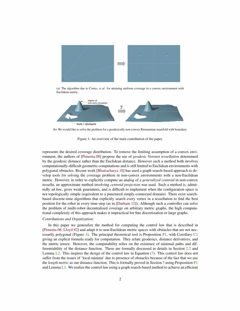
(a) The algorithm due to Cortes, et al. for attaining uniform coverage in a convex environment withEuclidean metric.

?

hole / obstacle

region ofnon-zero curvature

(b) We would like to solve the problem for a geodesically non-convex Riemannian manifold with boundary.

Figure 1: An overview of the main contribution of the paper.

represents the desired coverage distribution. To remove the limiting assumption of a convex envi-ronment, the authors of [Pimenta 08] propose the use of geodesic Voronoi tessellation determinedby the geodesic distance rather than the Euclidean distance. However such a method both involvescomputationally-difficult geometric computations and is still limited to Euclidean environments withpolygonal obstacles. Recent work [Bhattacharya 10] has used a graph search-based approach to de-velop tools for solving the coverage problem in non-convex environments with a non-Euclideanmetric. However, in order to explicitly compute an analog of a generalized centroid in non-convextessella, an approximate method involving centroid projection was used. Such a method is, admit-tedly ad hoc, gives weak guarantees, and is difficult to implement when the configuration space isnot topologically simple (equivalent to a punctured simply-connected domain). There exist search-based discrete-time algorithms that explicitly search every vertex in a tessellation to find the bestposition for the robot in every time-step (as in [Durham 12]). Although such a controller can solvethe problem of multi-robot decentralized coverage on arbitrary metric graphs, the high computa-tional complexity of this approach makes it impractical for fine discretization or large graphs.

Contributions and Organization:

In this paper we generalize the method for computing the control law that is described in[Pimenta 08, Lloyd 82] and adapt it to non-Euclidean metric spaces with obstacles that are not nec-essarily polygonal (Figure 1). The principal theoretical tool is Proposition P1, with Corollary C1giving an explicit formula ready for computation. They relate geodesics, distance derivatives, andthe metric tensor. However, the computability relies on the existence of minimal paths and dif-ferentiability of the distance function. These are formally discussed in details in Section 2.2 andLemma L2. This inspires the design of the control law in Equation (7). This control law does notsuffer from the issues of ‘local minima’ due to presence of obstacles because of the fact that we usethe length metric as our distance function. This is formally proved in Section 3 using Proposition P1and Lemma L1. We realize the control law using a graph search-based method to achieve an efficient

2

discrete implementation. We illustrate our methodology by showing how to solve Coverage prob-lems on non-Euclidean Riemannian manifolds with boundary, multi-robot cooperative exploration,and cooperative human-robot exploration.

In Section 2 of the paper we primarily discuss some mathematical tools related to Riemannianmanifolds with boundary. The main contribution of the paper appears in Section 3 where we developand prove stability of the proposed control law for coverage on Riemannian manifolds with bound-ary. We present the graph search-based discrete implementation and simulation results in Section 4.For better readability, we have placed the proofs of the lemmas, the corollary and the proposition inthe paper in the appendix at the end of the paper.

2 Background – Manifolds with BoundaryIn this section we discuss and build some of the theoretical tools that will be essential in designingand proving the stability of the control law (which we will do in Section 3) for coverage in generalRiemannian manifolds with boundary.

2.1 Motivation: Stability and Convergence of Control LawsIf the configuration space of a robot (or a system of robots) can be described by a Banach space (i.e. avector space with a norm, ‖·‖), one can easily specify convergence and stability of a proposed controllaw. In particular, Lyapunov stability, asymptotic stability and exponential stability [Sastry 99] aresome of the conditions that are often desired. These stability analyses often boil down to findingan energy-like function (often called the Lyapunov function), and showing that the proposed controllaw can be expressed as the gradient of the energy-like function. Conditions on the function and itsgradients on the entire space translate into stability conditions.

However, very often the configuration space under consideration is a general Riemannian man-ifold. If it is a complete manifold (i.e. every geodesic curve on it can be extended indefinitely inboth directions), one approach is to consider the tangent space at a point [Petersen 06], which is aHilbert space (and hence a Banach space), and study the local stability of the control laws in thetangent space via the exponential map. Since the exponential map is often not bijective, especiallyfor compact manifolds, the study of convergence in terms of Lyapunov function makes sense onlylocally at each point.

However the scenario is most difficult when the manifold is not complete. These are typicallymanifolds obtained by removing closed sets from other complete manifolds. In such cases theexponential map is not even defined completely on the entire tangent space at a point. Geodesicemanating from a point can hit a hole/puncture on the manifold. We often include the boundarynear the holes/punctures to make it a manifold with boundaries. That makes it complete as a metricspace, but it no longer remains a manifold since the points at the boundary do not locally resembleEuclidean space. Thus we lose the notion of a tangent bundle on this space with the tangent spacebeing fibers that are identical at every point.

Unfortunately it is the last kind of spaces that one encounters most often in problems of robotnavigation. The holes or punctures arise due to presence of obstacles. Supposing one can embedthe manifold with boundaries in an Banach space, stability of control laws on the embedding spacedoes not correspond to stability on the manifold with punctures.

The simplest example is that of a point robot navigating on R2, and the objective being reachinga goal point, pg ∈ R2. One can simply construct a smooth energy function, E : R2 → R, with anunique global minima at pg , and non-zero gradient everywhere else (e.g. E(r) = ‖(r−pg)‖2). The

3

ℝ2

r = -∇ℇ

pg

(a) Point robot at r navigating towards pg inthe Banach space, R2, by descending gradi-ent of E , will reach its goal.

O

ℝ2 − O

r = -∇ℇ

pg

(b) R2 − O is not a Banach space. On thisspace the integral curve of r = −∇E doesnot exist.

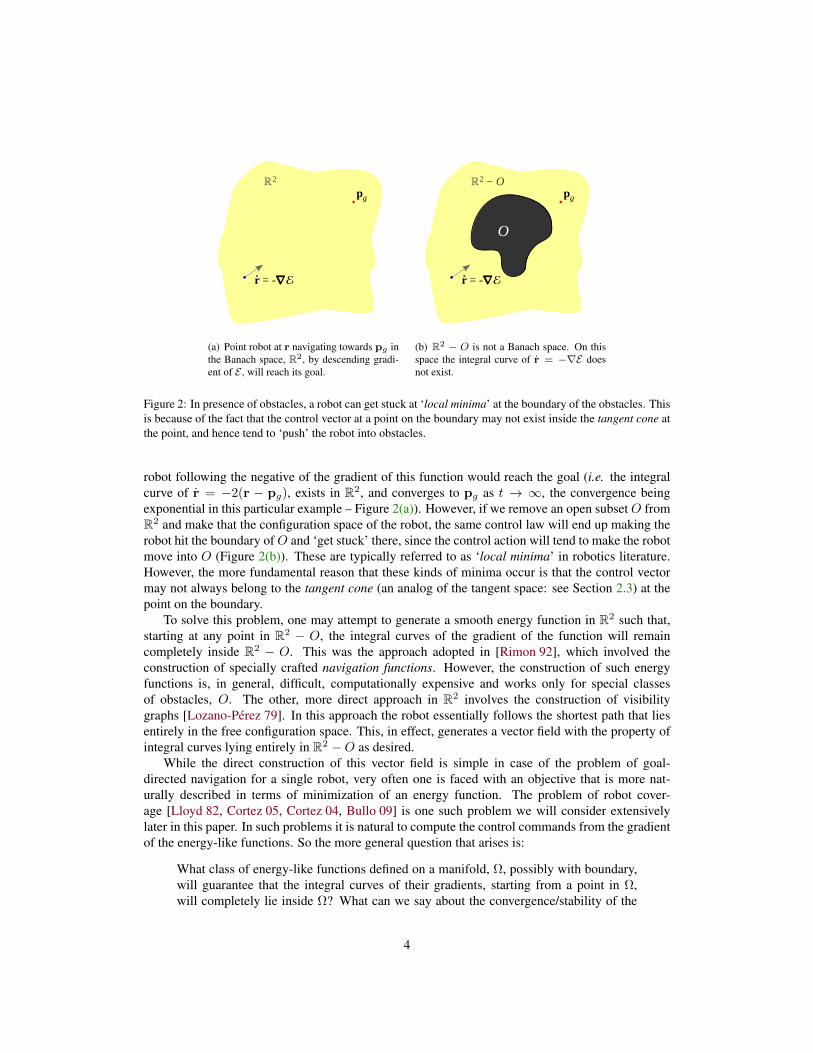
Figure 2: In presence of obstacles, a robot can get stuck at ‘local minima’ at the boundary of the obstacles. Thisis because of the fact that the control vector at a point on the boundary may not exist inside the tangent cone atthe point, and hence tend to ‘push’ the robot into obstacles.

robot following the negative of the gradient of this function would reach the goal (i.e. the integralcurve of r = −2(r − pg), exists in R2, and converges to pg as t → ∞, the convergence beingexponential in this particular example – Figure 2(a)). However, if we remove an open subset O fromR2 and make that the configuration space of the robot, the same control law will end up making therobot hit the boundary ofO and ‘get stuck’ there, since the control action will tend to make the robotmove into O (Figure 2(b)). These are typically referred to as ‘local minima’ in robotics literature.However, the more fundamental reason that these kinds of minima occur is that the control vectormay not always belong to the tangent cone (an analog of the tangent space: see Section 2.3) at thepoint on the boundary.

To solve this problem, one may attempt to generate a smooth energy function in R2 such that,starting at any point in R2 − O, the integral curves of the gradient of the function will remaincompletely inside R2 − O. This was the approach adopted in [Rimon 92], which involved theconstruction of specially crafted navigation functions. However, the construction of such energyfunctions is, in general, difficult, computationally expensive and works only for special classesof obstacles, O. The other, more direct approach in R2 involves the construction of visibilitygraphs [Lozano-Perez 79]. In this approach the robot essentially follows the shortest path that liesentirely in the free configuration space. This, in effect, generates a vector field with the property ofintegral curves lying entirely in R2 −O as desired.

While the direct construction of this vector field is simple in case of the problem of goal-directed navigation for a single robot, very often one is faced with an objective that is more nat-urally described in terms of minimization of an energy function. The problem of robot cover-age [Lloyd 82, Cortez 05, Cortez 04, Bullo 09] is one such problem we will consider extensivelylater in this paper. In such problems it is natural to compute the control commands from the gradientof the energy-like functions. So the more general question that arises is:

What class of energy-like functions defined on a manifold, Ω, possibly with boundary,will guarantee that the integral curves of their gradients, starting from a point in Ω,will completely lie inside Ω? What can we say about the convergence/stability of the

4

x

y

O

d(x, y)

dℓ (x, y)

Ω = (ℝ2 − O) ∪ ∂O

Figure 3: In this figure O represents a compact obstacle with smooth boundary in R2. Ω = (R2 − O) ∪ ∂Ois a manifold with smooth boundary that is complete as a metric space. The metric induced by R2 is not a pathmetric since a path of length d(x, y) does not exist in Ω. But d` is a path metric.

system?

While in this paper we will mostly focus on the problem of multi-robot coverage, we hope thatthe analysis that we will present in the following sections will help in establishing a much broadercontrol paradigm on manifolds with boundary.

2.2 Length MetricWe consider a smooth manifold, Ω, possibly with boundary. Such spaces are well-studied in math-ematics [Wolter 85, Alexander 81]. In robotics they are of great interest since they represent con-figuration spaces of many robots and linkages with no “immaterial edge” assumptions. For mostof the analysis in this paper we will assume that Ω is embedded in some Euclidean space equippedwith its standard Euclidean metric (RD, d). The topology of Ω is assumed to be the subspacetopology [Munkres 99] derived from RD (so that the boundary of Ω is part of the same topologicalspace). The metric induced by the ambient Euclidean space is, in general, not a path metric unlessΩ is convex (see p.10 of [Gromov 99]). That means, if i : Ω → RD is the embedding, for any pointsp, q ∈ Ω, there may not exist a path [0, 1]→ Ω of length d(i(p), i(q)).

However, if Ω is path connected, one can define a different metric structure on Ω that makesit a path metric space, (Ω, d`). The new metric, d`, called the length metric, can be defined suchthat d`(p, q) is the infimum of the length of rectifiable curves or paths (computed using the lengthstructure [Gromov 99] induced by the embedding) joining p and q, but lying entirely in Ω. It is notdifficult to see that (Ω, d`) is a complete metric space (though not geodesically complete). Thus,due to the Hopf-Rinow theorem [Gromov 99] there exists a minimizing path (not necessarily unique)joining every pair of points. Although this last observation may appear somewhat trivial, it is easy toconstruct cases of non-compact manifolds where such minimizing geodesics may not exist (e.g., inFigure 3, consider RD −O, without the boundary of O – a path of length equal to the infimum doesnot exist in that space for the shown points x, y). Thus we cannot simply remove the boundariesfrom the space of interest.

5

2.3 Generalization of Tangent SpaceBy retaining the boundary, Ω no more remains a manifold in the strict sense. Neighborhoods ofpoints on the boundary of Ω (i.e., points on ∂Ω) resemble an Euclidean half space. However, Ω−∂Ωis indeed a manifold, although not complete. Thus, given p ∈ (Ω− ∂Ω), one can define the tangentspace Tp(Ω − ∂Ω) in its usual sense. However, we do not have the usual notion of a tangent spaceat points on ∂Ω.

Let us now consider a point, p ∈ Ω. The tangent space of the Euclidean space in which Ω isembedded is thus Ti(p)RD. Now we consider the subset of this tangent space that consists of thevectors (and their non-negative scalings) that are tangents to curves emanating from p and lyingentirely in Ω. That is, we define the cone,

TpΩ =⋃

v∈ΛpΩ

αv | α ≥ 0

where,

ΛpΩ =

(dγi

dt

∣∣t=0

)∂

∂xi

∣∣∣ γ : [0, a]→ RD, a > 0 are C1 paths parametrized by their lengths,with γ(0) = p, Img(γ) ⊆ Ω

Here trajectory, γ, has been represented using a coordinate system of choice on RD. We call TpΩthe tangent cone at p in Ω.

Lemma L1. If Ω is a smooth manifold embedded in RD, TpΩ is a half space in Ti(p)RD for p ∈ ∂Ω,and a full space for p ∈ (Ω− ∂Ω) (see Figure 4).

Remark R1. The above lemma can be generalized to assert that TpΩ will be a convex cone for pointson a wider class of manifolds with boundaries with corners (i.e. boundaries that are not necessarilysmooth). As long as the space is locally convex (i.e. for every point p ∈ Ω, there exists a openneighborhood, U , in Ω, such that the metric induced by d makes U a path metric space), TpΩ willbe a convex cone (Figure 4(c)).

Remark R2. We will allow ∂Ω to be not smooth (C1) at finite number of distinct points, wherethey may not be locally convex either. In our coverage problem such a point can at the worst be anunstable ‘local minima’, in which case we will rely on presence of small noise that would ‘push’the robot out that isolated point (see Section 3). Alternatively we can assume smoothness of theboundary to be a generic condition, wherein a boundary with finite and distinct set of non-smoothpoints can be smoothened locally (using a mollifier) to obtain a C1 boundary. In which case theresult of Lemma L1 will hold for every point.

Remark R3. We define the cotangent cone at p as the dual of the cone TpΩ, and represent it as T ∗pΩ.If TpΩ is convex, so is T ∗pΩ, and vise-versa. Consider a real-valued smooth function, f : Ω → R.A differential of f is defined as an element of T ∗pΩ in usual way at points that lie in (Ω − ∂Ω). Todefine a differential at a point p that lies on ∂Ω, we take a Cauchy sequence of points in Ω − ∂Ωthat converges to p (recall that Ω is a complete metric space). The limit of the differentials of fin the cotangent cones of these points gives us the required differential at p. This limit, however,may or may not exists in T ∗pΩ, and that will depend on the nature of f . The gradient of f is thecorresponding dual of the differential in TpΩ.

6

O

Ω = (ℝ2 − O) ∪ ∂O

(a) In the interior of Ω,neighborhoods are Euclideanspace, which is convex.

O

Ω = (ℝ2 − O) ∪ ∂O

(b) On smooth boundary ofΩ, neighborhoods are Eu-clidean half space, which isconvex.

O

Ω = (ℝ2 − O) ∪ ∂O

(c) Although this is a pointon the boundary where it isnot C1, TpΩ is still convex.

O

Ω = (ℝ2 − O) ∪ ∂O

(d) TpΩ is not convex at thispoint.

Figure 4: Points on Ω and the shape of TpΩ (the pale yellow region inside the circle). (a), (b) show Ω withsmooth boundary. (c), (d) show Ω with non-smooth boundary.

2.4 Cut LocusDefinition D1 (Cut locus on manifolds with boundary – See Definition 3.4.II of [Wolter 85]). Letp ∈ Ω. A point, q ∈ (Ω − ∂Ω), is called a pica relative to p if p and q can be joined with two ormore distinct minimal paths (i.e. paths of length d`(p, q)) with distinct tangents at q. The closure ofthe set of all picas relative to p is called the cut locus of p and is denoted by Cp (Figure 5(a)).

Note that by using the term ‘distinct minimal paths’ we mean to impose the condition that theimage of any two distinct paths are not the same. This excludes the multiplicity of paths due to merere-parameterization. The definition of cut locus in terms of ‘pica’ (equivalently, non-extenders) isnecessary for retaining certain properties of the standard cut locus on manifolds without boundaries.

Lemma L2 (Wolter [Wolter 85]). If Ω is a smooth manifold (with boundaries), which is complete asa metric space, and can be defined as a subset of a smooth, complete manifold of same dimension,then for every p ∈ Ω,

i. Cp is a closed set of measure zero in Ω,

ii. the function gp := d`(p, ·) is of class C1 in Ω− (∂Ω ∪ p ∪ Cp), and

iii. the gradient of gp is bounded in Ω− (∂Ω ∪ p ∪ Cp).

Lemma L3. For almost every point p ∈ Ω: q /∈ Cp =⇒ p /∈ Cq

7

p

pΩ

(a) Points on Cp can be joined with p using 2 minimalgeodesics.

p

Ω q

dℓ(p,q)

q'

(b) On points on the dotted line in this figure (e.g. thepoint q′), gp is C1, but not C2.

Figure 5: The cut locus of p and the smoothness of the function gp.

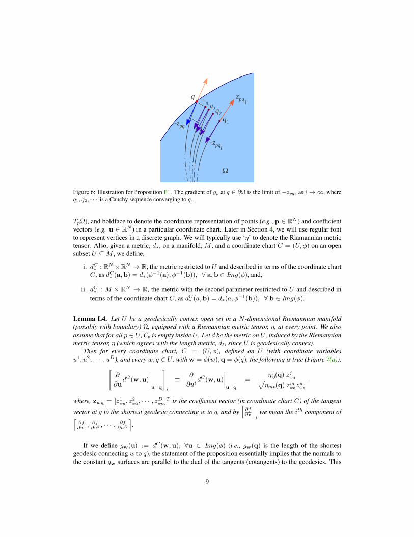
2.5 Gradient of Distance FunctionProposition P1. Let p ∈ Ω. The negative of the gradient of gp := d`(p, ·) exists in TqΩ (equiva-lently, the negative of the differential of gp exists in T ∗q Ω) at all points q ∈ Ω − (p ∪ Cp) that areequipped with a Riemannian metric in their neighborhoods. The negative of the gradient is equal toa normalized vector at q along the tangent to the minimal path connecting q to p (equivalently, thedifferential is the dual of the unit tangent vector along the minimal path).

Remark on existence: If q is a point in Ω − (∂Ω ∪ p ∪ Cp), the gradient (and its negative)obviously exist in TqΩ (part ‘ii.’ of Lemma L2). We need to check the existence for points on theboundary ∂Ω. Recall that for points, q ∈ ∂Ω, we defined the gradient of a function as the limit ofthe gradients over a Cauchy sequence of points, qn, in Ω − (p ∪ ∂Ω ∪ Cp) converging to q. Wecan prove the later half of the statement for each of these qn (i.e. that the negative of the gradient isequal to a normalized vector at qn along the tangent to the minimal path connecting qn to p). Then,the existence of the negative of the gradient at q is implied by the existence of the minimal path.Since the tangent to the minimal path connecting q to p exists in TqΩ (by definition of the tangentcone), the negative of the gradient will also exist (see Figure 6).

Thus, the proof of the above proposition relies on being able to compute the gradient of gpat q ∈ Ω − (p ∪ ∂Ω ∪ Cp) in terms of the tangent to the minimal path. Using the lemma andcorollary that follows next, we will establish an explicit relationship between the gradient of gpand tangents to minimal paths using a coordinate representation of the metric tensor, and usingthese will be able to prove the Proposition P1. We will assume summation over repeated indicesfollowing the Einstein summation convention, and coordinatize tangent spaces and the cotangentspaces by ∂

∂xi i=1,2,··· ,N and dxii=1,2,··· ,N respectively [Jost 97, Petersen 06].

Notations: We will use regular italic letters to denote points and vectors (e.g p ∈ Ω and u ∈

8

q1

q2

q3q4

...q ...

...

-zpqi

-zpq

zpq1

Ω

Figure 6: Illustration for Proposition P1. The gradient of gp at q ∈ ∂Ω is the limit of −zpqi as i → ∞, whereq1, q2, · · · is a Cauchy sequence converging to q.

TpΩ), and boldface to denote the coordinate representation of points (e.g., p ∈ RN ) and coefficientvectors (e.g. u ∈ RN ) in a particular coordinate chart. Later in Section 4, we will use regular fontto represent vertices in a discrete graph. We will typically use ‘η’ to denote the Riamannian metrictensor. Also, given a metric, d∗, on a manifold, M , and a coordinate chart C = (U, φ) on an opensubset U ⊆M , we define,

i. dC∗ : RN ×RN → R, the metric restricted to U and described in terms of the coordinate chartC, as dC∗ (a,b) = d∗(φ

−1(a), φ−1(b)), ∀ a,b ∈ Img(φ), and,

ii. dC∗ : M × RN → R, the metric with the second parameter restricted to U and described interms of the coordinate chart C, as dC∗ (a,b) = d∗(a, φ

−1(b)), ∀ b ∈ Img(φ).

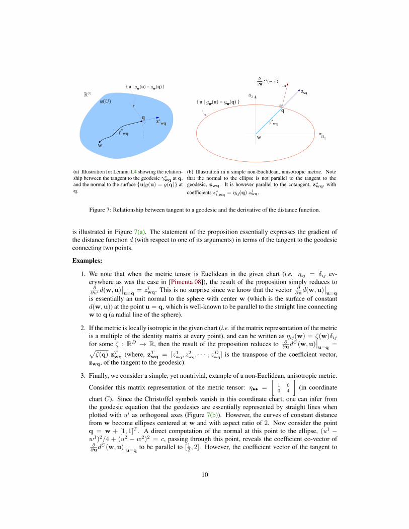
Lemma L4. Let U be a geodesically convex open set in a N -dimensional Riemannian manifold(possibly with boundary) Ω, equipped with a Riemannian metric tensor, η, at every point. We alsoassume that for all p ∈ U , Cp is empty insideU . Let d be the metric onU , induced by the Riemannianmetric tensor, η (which agrees with the length metric, d`, since U is geodesically convex).

Then for every coordinate chart, C = (U, φ), defined on U (with coordinate variablesu1, u2, · · · , uD), and every w, q ∈ U , with w = φ(w),q = φ(q), the following is true (Figure 7(a)),[

∂

∂udC(w,u)

∣∣∣∣u=q

]i

≡ ∂

∂uidC(w,u)

∣∣∣∣u=q

=ηij(q) zjwq√ηmn(q) zmwqz

nwq

where, zwq = [z1wq, z

2wq, · · · , zDwq]T is the coefficient vector (in coordinate chart C) of the tangent

vector at q to the shortest geodesic connecting w to q, and by[∂f∂u

]i

we mean the ith component of[∂f∂u1 ,

∂f∂u2 , · · · , ∂f

∂uD

].

If we define gw(u) := dC(w,u), ∀u ∈ Img(φ) (i.e., gw(q) is the length of the shortestgeodesic connecting w to q), the statement of the proposition essentially implies that the normals tothe constant gw surfaces are parallel to the dual of the tangents (cotangents) to the geodesics. This

9

w

qz*

wq

u | w(u) = w(q)

?

γ*wq

φ(U)ℝN

(a) Illustration for Lemma L4 showing the relation-ship between the tangent to the geodesic γ∗wq at q,and the normal to the surface u|g(u) = g(q) atq.

w

q

u | w(u) = w(q)

zwq

u1

u2

γ*wq

(b) Illustration in a simple non-Euclidean, anisotropic metric. Notethat the normal to the ellipse is not parallel to the tangent to thegeodesic, zwq. It is however parallel to the cotangent, z∗wq, with

coefficients z∗i,wq= ηij(q) zjwq.

Figure 7: Relationship between tangent to a geodesic and the derivative of the distance function.

is illustrated in Figure 7(a). The statement of the proposition essentially expresses the gradient ofthe distance function d (with respect to one of its arguments) in terms of the tangent to the geodesicconnecting two points.

Examples:

1. We note that when the metric tensor is Euclidean in the given chart (i.e. ηij = δij ev-erywhere as was the case in [Pimenta 08]), the result of the proposition simply reduces to∂∂ui d(w,u)

∣∣u=q

= ziwq. This is no surprise since we know that the vector ∂∂ud(w,u)

∣∣u=q

is essentially an unit normal to the sphere with center w (which is the surface of constantd(w,u)) at the point u = q, which is well-known to be parallel to the straight line connectingw to q (a radial line of the sphere).

2. If the metric is locally isotropic in the given chart (i.e. if the matrix representation of the metricis a multiple of the identity matrix at every point), and can be written as ηij(w) = ζ(w)δijfor some ζ : RD → R, then the result of the proposition reduces to ∂

∂udC(w,u)

∣∣u=q

=√ζ(q) zTwq (where, zTwq = [z1

wq, z2wq, · · · , zDwq] is the transpose of the coefficient vector,

zwq, of the tangent to the geodesic).

3. Finally, we consider a simple, yet nontrivial, example of a non-Euclidean, anisotropic metric.

Consider this matrix representation of the metric tensor: η•• =

[1 00 4

](in coordinate

chart C). Since the Christoffel symbols vanish in this coordinate chart, one can infer fromthe geodesic equation that the geodesics are essentially represented by straight lines whenplotted with ui as orthogonal axes (Figure 7(b)). However, the curves of constant distancefrom w become ellipses centered at w and with aspect ratio of 2. Now consider the pointq = w + [1, 1]T . A direct computation of the normal at this point to the ellipse, (u1 −w1)2/4 + (u2 − w2)2 = c, passing through this point, reveals the coefficient co-vector of∂∂ud

C(w,u)∣∣u=q

to be parallel to [ 12 , 2]. However, the coefficient vector of the tangent to

10

the geodesic is zwq = [ 1√2, 1√

2]T . This gives the following:

√ηmn(q) zmwqz

nwq =

√52 ,

z1,wq =∑j η1j z

jwq = 1√

2, z2,wq =

∑j η2j z

jwq = 2

√2. Thus, the coefficient co-vector of

z∗wq is parallel to [ 1√2, 2√

2]. This indeed is parallel to [ 12 , 2]. The exact computation of the

scalar multiple will require a more careful computation of ∂∂ud

C(w,u).

In the following corollary we relax some conditions imposed on U in the Lemma L4 so that wecan generalize the result to manifolds that are not necessarily geodesically convex.

Corollary C1. Let Ω be a N -dimensional manifold possibly with boundaries, which is complete asa metric space, with length metric d`. Let p ∈ Ω and q ∈ Ω− (p ∪ ∂Ω ∪ Cp). Let q be such that themetric in its neighborhood is induced by a Riemannian metric tensor, η. Let d` be the length metricon Ω.

Then the following holds for every coordinate chart, D = (V, ψ), defined on open set V 3 q,[∂

∂udD` (p,u)

∣∣∣∣u=q

]i

≡ ∂

∂uidD` (p,u)

∣∣∣∣u=q

=ηij(q) zjpq√ηmn(q) zmpqz

npq

where, q = ψ(q), and zpq = [z1pq, z

2pq, · · · , zDpq]T is the coefficient vector (in coordinate chart D) of

the tangent vector at q to the shortest geodesic connecting p ∈ Ω to q ∈ V . By[∂f∂u

]i

we mean the

ith component of[∂f∂u1 ,

∂f∂u2 , · · · , ∂f

∂uD

].

Remark R4. This Corollary is applicable to a wider class of metric spaces than Lemma L4. Here weonly need to assume a Riemannian metric in the neighborhood of q (Figure 8(a)). This will enable usto use the result for locally Riemannian manifolds allowing for pathologies outside local neighbor-hoods (e.g. boundaries/holes/punctures/obstacles – the kind of spaces we are most interested in), aswell as opens up possibilities for more general metric spaces that may not be Riemannian outside asmall ball neighborhood of q, Bq (e.g. Manhattan metric inM⊂ Ω, Riemannian metric elsewhere).However, in this paper we will not consider the later kind of cases.

Examples:

1. The simplest example of a space that is only locally Euclidean is one that is R2 puncturedby polygonal obstacles (Figure 8(b)). Due to the ‘pointedness’ of the obstacles, the constant-gp manifolds are essentially circular arcs centered at p or a vertex v of a polygon. Thus, asillustrated by Figure 8(b), the normals to the arcs are parallel to the tangent to the segmentjoining v to q.

2. A less trivial case is seen in the example where the obstacles have curved boundaries. Thenthe corollary essentially reduces to the assertion that the normal at any point on an invo-lute [Cundy 89] is parallel to the ‘taut string’, the end of which traces the involute – and thisis true irrespective of the curve used to generate the involute. While the statement has anobvious intuitive explanation by considering the possible directions of motion of the end ofthe taut string, we provide an explicit computation for an involute created using a circle (Fig-ure 8(c)). Consider a taut string unwrapping off a circle of radius r (starting from θ = 0 whenit is completely wrapped). Thus, when the string has unwrapped by an angle θ, the string

11

p

w

q

V q

Ω

(a) Illustration for Corollary C1. The patholo-gies outside Bq do not effect the result ofLemma L4 holding for p and q.

p

q

z*pq

ψ-1( u | p(u) = p(q) )

v

(b) Example of a space that is equipped withEuclidean metric everywhere, but is puncturedby a polygonal obstacles. Here the gp(q) =const. curve consists of circular arcs. Thiswas the case considered in [Pimenta 08].

p

q

z*pqψ-1( u | p(u) = p(q) )

x

y

θ

(c) An example with a circular obstacle wherethe gp(q) = const. curve consists of an invo-lute and circular arc.

(x, y)

Y

X1

Manhattan

Euclidean

p

q

α

2

v

(d) An example involving Manhattan and Eu-clidean metrics in two different regions. Thedistance function between points lying in thetwo different regions is given by d(p,q) =minv (dman(p,v) + deu(v,q)), where v is apoint lying on the boundary of the two regions.

Figure 8: Corollary C1 and illustrative examples.

12

-2

-1

0

1

2

3

-2 -1 0 1 2 3

Figure 9: Voronoi tessellation of a convex Ω (rectangular region) with n = 10 robots (blue circles). The red linesegments show the boundary of the tessellation. Note how a boundary segment is the perpendicular bisector ofthe cyan line joining the robots sharing the boundary segment.

points at a direction [sin(θ),− cos(θ)]T . Now, it is easy to verify that the involute is describedby the parametric curve x = r(cos(θ) + θ sin(θ)), y = r(sin(θ) − θ cos(θ)). Thus we havedxdθ = θ cos(θ), dy

dθ = θ sin(θ). Thus the normal to the involute pointing in the direction[ dy

dθ ,−dxdθ ] is indeed parallel to the direction in which the string points.

3. The last example that we will illustrate involves a mixture of Manhattan distance (in a par-ticular given coordinate chart) and Euclidean metric. Consider the case in Figure 8(d),where in the given coordinate chart p is the origin, (0, 0). For any two points inside thehalf-plane M = (x, y)|2x + y < 2, the distance function is the Manhattan distance.Outside M it is induced by Euclidean metric. It is to be noted that although the distancefunction is defined in M, geodesics are not uniquely defined. Let us consider the pointq = (x, y) outsideM (so that there exists a Bq as required by Corollary C1). The distance

is given by d(p,q) = minα∈R

(α+ 2(1− α) +

√(x− α)2 + (y − 2(1− α))2

). Denoting

the quantity inside ‘min’ by f(α), and by solving ∂f∂α = 0, one obtains the unique solution

α = (4x − 3y + 6)/10. This gives d(p,q) = (3x + 4y + 12)/5. Thus, the normals to theconstant-d surfaces are parallel to [3/5, 4/5]. Again, the segments vq have tangent pointingin the direction [x− α, y − 2(1− α)]T = [(6x+ 3y − 6)/10, (8x+ 4y − 8)/10]T . Thus wesee that they are indeed parallel.

3 The coverage problem in roboticsBackground: In this section we discuss the derivation of the control laws in the continuous-time

version of the Lloyd’s algorithm. We start with the classical case for convex environments withEuclidean metric [Lloyd 82], and from that motivate our generalization to general manifolds withboundary and general Riemannian metric.

Let Ω be a path-connected metric space that represents the environment, equipped with a metric,d∗ : Ω × Ω → R+. In [Lloyd 82, Pimenta 08] Ω is assumed to be a convex subset of RN andis equipped with the Euclidean metric tensor at every point. However, in the present scenario werelax d∗ to a more general metric on a metric space, Ω, that need not necessarily be a manifold. Wewill eventually consider the length metric, d`, on manifolds with boundary, induced by a generalRiemannian metric. We will introduce those restrictions gradually as they are required.

13

Coverage functional: Suppose there are n mobile robots in Ω. The position of the kth robot isrepresented by pk ∈ Ω. By definition, a tessellation [Lloyd 82, Pimenta 08] of the environment is apartition of Ω, written as Wkk=1,2,··· ,n, such that each Wk (called a tessella) is path connected,pk ∈ Wk, Int(Wk) ∩ Int(Wl) = ∅,∀k 6= l, and ∪nk=1Wk = Ω. The tessella associated with thekth robot is Wk,∀k = 1, 2, . . . , n. For a given set of robot positions P = p1, p2, . . . , pn andtessellation W = W1, W2, . . . , Wn, the coverage functional is defined as:

H(P,W ) =

n∑k=1

H(pk,Wk) =

n∑k=1

∫Wk

fk(d∗(q, pk)) w(q) dq (1)

where fk : R+ → R are smooth and strictly increasing functions,w : Ω→ R+ is a weight or densityfunction, and dq represents an infinitesimal volume element (more formally, it is a top-dimensionalmeasure of an an infinitesimal element, associated with the metric d∗ [Gromov 99]).

The name “coverage functional” is indicative of the fact thatH measures how bad the coverageis — i.e., more well-distributed the robots are throughout the environment, lower is the value ofH. In fact, for a given set of initial robot positions, P , we devise a control law that minimizes thefunction H(P ) := min

WH(P,W ) (i.e. the best value of H(P,W ) for a given P ). It is easy to

show [Lloyd 82, Pimenta 08] that H(P ) = H(P, V ), where V = V1, V2, · · · , Vn is the Voronoitessellation given by

Vk = q ∈ Ω | fk(d∗(q, pk)) ≤ fl(d∗(q, pl)),∀l 6= k (2)

Requiring Ω to be a manifold with boundary: The control law for minimizing H(P ) =∑nk=1

∫Vkfk(d∗(q, pk))w(q) dq can be reduced to the problem of moving along the direction of

its steepest descent. So far in this section we have not required that Ω be a manifold. However, wewould like to be able to compute the gradient of H(P ) so that the negative of it is the direction ofsteepest descent. It suffices that the configuration space be a manifold so that each point on it has atangent space in which the gradient of a function (or its negative) will reside. However, based on ourdiscussions in Section 2, we are now capable of defining and computing gradients on manifolds withboundary (see Remark R3). However, we need to check the existence of the negative of the gradientinside the tangent cone at a point on the boundary, so that the robots can move along that direction.In the following discussion we use explicit coordinate charts, Ck = (Uk, φk), with pk ∈ Uk —the position of the kth robot, at which we compute the gradients. Using the notation introduced inCorollary C1, we write dCk

∗ (a,b) := d∗(a, φ−1k (b)) for b ∈ Img(φk).

The domains of integration, Vk are functions of P , and hence the gradient of H(P ) would, ingeneral, involve boundary terms, ∂Vk. However, it can be shown using methods of differentiationunder integration [Pimenta 08] that the boundary terms vanish. So the final formula for the partialderivatives of H(P ) with respect to the position of the robots become,

∂H(P )

∂pk=

∫Vk

∂

∂pkfk(dCk

∗ (q,pk)) w(q) dq (3)

In practice, it is adequate to choose fk(x) = x2 for most implementations [Cortes 04]. However,a variation of the problem for taking into account finite sensor footprint of the robots, constructs apower Voronoi tessellation [Pimenta 08], in which one chooses fk(x) = x2 − R2

k, where Rk canrepresent, for example, the radius of the sensor footprint of the kth robot. In this paper we will beworking with the following form for fk

fk(x) = x2 + ck (4)

14

Requiring d∗ to be a metric induced by Riemannian metric tensor: Until now we haven’t madeany major assumption on the distance function d∗ besides the fact that it is a metric on a manifoldwith boundaries that can be differentiated at the points pk. We next impose the condition that themetric is locally represented by a Riemannian metric tensor, η.

Remark R5. If the space Ω is convex, and we can construct a single coordinate chart, B =Ω, ψ, over entire Ω such that the matrix representation of the metric tensor is Euclidean every-where, then d∗ is the Euclidean distance given by dB∗ (x,y) = ‖x − y‖2 (where, dB∗ (a,b) =d∗(ψ

−1(a), ψ−1(b)) – refer to notation introduced in Lemma L4). This was the case consideredin [Lloyd 82] (see Figure 9). Under this assumption, and using the form of fk in (4), the formulaof (3) can be simplified to obtain

∂H(P )

∂pk= 2Ak(pk − p∗k) (5)

where, Ak =∫Vkw(q) dq is the weighted volume of Vk, and p∗k =

∫Vk

q w(q) dq

Ak(with

q = ψ(q), the coordinate representation of q) is the weighted centroid of Vk. Moreover,the Euclidean distance function makes computation of the Voronoi tessellation very easy: V ,due to Equation (2), can be constructed from the perpendicular bisectors of the line segmentspkpl, ∀k 6= l in the coordinate chart B, thus making each Vk a convex polygon, which are alsosimply connected (Figure 9). This also enable closed-form computation of the volume, Ak, andthe centroid, p∗k when the weight function, w, is uniform. Equation (5) yields the simple controllaw (in coordinate chart B) in continuous-time Lloyd’s algorithm: uk = −κAk(pk − p∗k), withsome positive gain, κ. Lloyd’s algorithm [Lloyd 82] and its continuous-time asynchronous im-plementations [Cortes 04] are distributed algorithms for minimizing H(P,W ) with guaranteeson completeness and asymptotic convergence to a local optimum, when Ω is convex Euclidean.However, this simplification does not work when there does not exist a coordinate chart as B inwhich the metric can be expressed as the Euclidean norm of difference for every pair of points— an inherent characteristic of spaces with holes/obstacles or with metric that is intrinsicallynon-Euclidean.

Requiring d∗ to be the length metric: We also impose the condition that the metric be the lengthmetric, i.e. d∗ = d`, that was introduced in Section 2.2. In the following discussion we will henceuse results derived in Section 2 to make assertions about the existence of the gradient, and hence theconvergence.

Now, with fk(x) = x2 + ck, we have ∂∂pk

fk(dCk

` (q,pk)) = 2 d`(q, pk) ∂∂pk

dCk

` (q,pk) where,pk = φk(pk). Substituting this into Equation (3) and using Proposition P1 (with the explicit formulafrom Corollary C1) we obtain,[

∂H(P )

∂pk

]i

= 2

∫Vk

d`(q, pk)∂

∂pkdCk

` (q,pk) w(q) dq

= 2

∫Vk−(p∪Cpk )

d`(q, pk)ηij(pk) zjqpk√ηmn(pk) zmqpk

znqpk

w(q) dq (6)

where zjqpkis the jth component of the coefficient vector (in coordinate chart Ck) of the tangent at

pk to the minimal path connecting q and pk.That we can write the second equality is due to the fact that pk∪Cpk is a set of measure zero in Vk

(a consequence of Lemma L2), outside which ∂∂pk

dCk

` (·,pk) exists (a consequence of Proposition P1

15

and and Lemma L3): The domain of integration in the second integral implies q /∈ Cpk . This, due toLemma L3, implies that pk /∈ Cq almost always (i.e. for all pk, except possibly for a set a measurezero in Ω). Also, pk 6= q. This, due to Proposition P1, implies the gradient of d`(q, ·) exists at pk.Thus we could write the quantity inside the second integral. Moreover, due to part ‘i’ of Lemma L2,pk ∪Cpk is a set of measure zero in Vk (since Vk is not a set of measure zero in Ω). Also, due to part‘iii.’ of the same lemma, the gradient at the points in the neighborhoods of pk ∪ Cpk is finite. Thus,removing pk ∪ Cpk from the domain of integration does not change the value of the integral, but letsus compute the integral.

We consider the negative of the quantity in (6). The[−∂H(P )

∂pk

]i

are coefficients (in chart Ck)of a covector that resides in T ∗pkΩ. The corresponding vector (the dual) will thus have coefficients[−∂H(P )

∂pk

]iηil(pk) (where η•• is matrix inverse of the matrix representation of the metric tensor,

η•• [Jost 97, Petersen 06]). This is the vector along which the kth robot needs to be moved forreducing the value of H the most. Using a scalar gain of κ and noting that ηijηil = δli, the lth

coefficients of the control vector for the kth robot will be

[uk]l =: ulk = κ

[−∂H(P )

∂pk

]i

ηil(pk)

= 2 κ

∫Vk−(p∪Cpk )

d`(q, pk)−zjqpk√

ηmn(pk) zmqpkznqpk

w(q) dq (7)

We now test if this vector actually exists in TpkΩ for all pk (including ones on ∂Ω). Clearly−zjqpk

∂∂xj exists in TpkΩ, since the minimal path connecting pk and q exists (see proof of Propo-

sition P1). Now we recall that TpkΩ is a convex cone almost everywhere in Ω due to Lemma L1and Remark R1 (except for possibly isolated points on ∂Ω, in which case we either smoothen theboundary near that point or rely on presence of small noise that would ‘push’ the robot out thatisolated point – see Remark R2). Thus a positive linear combination of vectors in TpkΩ (which thequantity in (7) is) will also be in TpkΩ. This essentially implies that if the kth robot follows thiscontrol law, it won’t get ‘stuck’ at a point on the boundary. It will stop only when the gradient of Hbecomes zero, making the control vector zero.

As discussed earlier, a single coordinate chart over entire Ω may not exists. However, for manycomputational purposes, one can use a single coordinate chart,B = (Ω−S, ψ), that describes almostthe whole of Ω, except for a set of measure zero, S (e.g. the polar coordinate on a sphere describeseverything except one longitudinal line and the poles). Thus, it is worth re-writing equation (7)entirely in terms of a coordinate chart. Besides changing q to q = ψ(q) and pk to pk = ψ(pk),we need to compute the volume of the infinitesimal element dq in the particular coordinate chart.Assuming dq to be an infinitesimal element in a particular coordinate chart, this is given by dq =√

det(η••(q)) dq. Thus we have,

ulk = 2κ

∫Vk−(p∪Cpk∪S)

dB` (q,pk)−zjqpk√

ηmn(pk) zmqpkznqpk

wB(q)√

det(η••(q)) dq (8)

where dB` is the length metric expressed in terms of coordinate chart B, i.e., dB` (a,b) =d`(ψ

−1(a), ψ−1(b)). Likewise, wB : RN → R+ such that wB(a) = w(ψ−1(a)). zqpk=

[z1qpk

, z2qpk

, · · · , zDqpk]T is the coefficient vector (in chartB) of the tangent vector at q to the minimal

path joining pk and q. We emphasize on the fact that (p ∪ Cpk ∪ S) is a set of measure zero in Ω,and does not concern us as far as computation is concerned.

16

The formula in (8), as we will see in the next section, gives an algorithm for approximately com-puting the gradient of H. This give a generalized Lloyd’s algorithm with guarantee of asymptoticstability (since we showed that the control vector will always exist in the tangent cones at points inΩ, and hence the only way the robots can stop is when the control becomes zero, i.e. the gradientof H vanishes). In the final converged solution, each robot will be at the generalized centroid of itsrelated Voronoi tessellation.

4 Graph Search-based Implementation

Figure 10: Graph construction: An 8-connected grid graph created from a uniformly discretized coordinatespace. The brown cells represent obstacles.

In order to develop a version of the generalized continuous-time Lloyd’s algorithm for a generaldistance function, we first need to be able to compute the general Voronoi tessellation of Equation (2)for the metric, d`. We adopt a discrete graph-search based approach for achieving that, not unlike theapproach taken in previous work [Bhattacharya 10]. We consider a uniform square tiling (Figure 10)of the space of coordinate variables (in a particular coordinate chart) and create a graph G out of it(with vertex set V(G), edge set E(G) ⊆ V(G) × V(G) and cost function CG : E(G) → R+). Thecosts/weights of the edges of the graph are the metric lengths of the edges. It is to be noted thatin doing so we end up restricting the metric of the original space to the discrete graph. Because ofthis, as well as due to the discrete computation of the integrations (as discussed later), this discretegraph-search based approach is inherently an approximate method, where we trade off the accuracyand elegance of a continuous space for efficiency and computability with arbitrary metric.

The key idea is to make a basic modification to Dijkstra’s algorithm [Dijkstra 59, Cormen 01].This enables us to create a geodesic Voronoi tessellation. For creating Voronoi tessellation weinitiate the open set with multiple start nodes from which we start propagation of the wavefronts.Thus the wavefronts emanate from multiple sources. The places where the wavefronts collide willhence represent the boundaries of the Voronoi tessellation. In addition, we can conveniently alter thedistance function, the level-set of which represents the boundaries of the Voronoi tessellation. Thisenables us to even create geodesic power Voronoi tessellation. Figure 11 illustrates the progress ofthe algorithm in creation of the tessellation.

In order to compute the control command for the robots (i.e. the action of the robot in the nexttime step), we use the formula in Equation (8). In a discretized setup, the position of the kth robotcorresponds to a vertex pk ∈ V(G) (note that we use a vertical, regular-weight font to distinguish avertex from the point pk ∈ Ω or its coordinate representation pk). The coefficient vector zqpk

of the

17

(a) iter = 1. (b) iter = 10100. (c) iter = 25100. (d) iter = 30100. (e) iter = 37300.

Figure 11: Progress of the algorithm for tessellation and control computation in an environment with a L-shaped obstacle. The graph is constructed by 200 × 200 uniform square discretization of the environment(see [Bhattacharya 10]). Tessellation is created starting from three points (the location of the agents) to thecomplete diagram after expansion of about 37300 vertices. The filled area indicates the set of expanded vertices.The boundaries of the tessellation are visible in blue.

tangent vector is approximated by the coefficient vectors along edges of the form [p′k,pk] ∈ E(G) forsome p′k ∈ NG(pk) (the set of neighbors of pk) such that the shortest path in the graph connectingpk and q ∈ V(G) passes through p′k. For a given q, we know the index of the robot, τ(q), whosetessella it belongs to, and can compute the shortest path in the graph joining the vertices pτ(q) andq. The neighbor of pτ(q), through which the shortest path passes, is the desired p′τ(q), and it ismaintained in a variable η(q) in an efficient way. Thus, we can also compute the integration of (8)on the fly (by approximating it as a summation over the discrete cells) as we compute the tessellation.The complete pseudo-code of the algorithm is given below.

τ, p′k = Tessellation and Control Computation (G, pk, Rk, w)Inputs: a. Graph G (with vertex set V(G), edge set E(G) ⊆ V(G)× V(G),

and cost function CG : E(G)→ R+)b. Agent locations pk ∈ V(G), k = 1, 2, · · · , nc. Agent weight Rk ∈ R+, k = 1, 2, · · · , Nd. Discretized weight/density function w : V(G)→ Re. The matrix representation of metric tensor, η.. : Img(ψ)→ RD×D , in coordinate chart B

Outputs: a. The tessellation map τ : V(G)→ 1, 2, · · · , nb. The next position of each robot, p′k ∈ NG(pk), k = 1, 2, · · · , n

1 Initiate g: Set g(v) :=∞, for all v ∈ V(G) // Shortest distances2 Initiate ρ: Set ρ(v) :=∞, ∀v ∈ V(G) // Power distances3 Initiate τ : Set τ(v) := −1, ∀v ∈ V(G) // Tessellation4 Initiate ν: Set ν(v) := ∅, ∀v ∈ V(G) // Pointer to robot neighbor. ν : V(G)→ V(G)5 for each (k ∈ 1, 2, · · · , n)6 Set g(pk) = 07 Set ρ(pk) = −R2

k

8 Set τ(pk) = k

9 Set Ik := 0 // The negative of differential of H in coordinate chart B (a covector).10 for each (q ∈ NG(pk)) // For each neighbor of pk11 Set ν(q) = q12 Set Q := V(G) // Set of un-expanded nodes13 while (Q 6= ∅)14 q := argminq′∈Q ρ(q′) // Maintained by a heap data-structure.15 if (g(q) ==∞)16 break17 Set Q = Q− q // Remove q from Q

18

18 Set l := τ(q)19 Set s := ν(q)20 if (s != ∅) // Equivalently, q /∈ pkk=1,2,...,n

21 Set z = P(s)−P(pl) // Negative of tangent vector21 Set M = η..(P(pl)) // Metric tensor at pl as a matrix in coordinate representation of B.21 Set Il += g(q)× Mz√

zTMz× w(q)×

√detM // Negative of integral in gradient of H

22 for each (w ∈ NG(q)) // For each neighbor of q23 Set g′ := g(q) + CG([q,w])24 Set ρ′ := PowerDist(g′, Rl)25 if (ρ′ < ρ(w))26 Set g(w) = g′

27 Set ρ(w) = ρ′

28 Set τ(w) = l29 if (s != ∅) // Equivalently, q /∈ pkk=1,2,··· ,n30 Set ν(w) = s31 for each (k ∈ 1, 2, · · · , n)32 Set p′k := argmaxu∈NG(pk) (P(u)−P(pk)) · Ik // Choose action best aligned along Ik.33 return τ, p′k

where, we used the coordinate chart B = (Ω−S, ψ) as discussed earlier. The function P : V(G)→Ω is such that P(q) gives the coordinate of the vertex q. Thus, P(pk) = pk and P(q) = q inrelation to Equation (8). In an uniform discretization setting we take w(q) = α w(ψ−1(P(q))) foran arbitrary positive constant α representing the ‘area’ of each discretized cell. Note that Ik is thecoefficient vector of the differential of H (a covector), while uk is its dual (a vector – see Equa-tion (7)). Thus, in line 32 of the algorithm, the ‘dot product’ is an element-wise product followedby a summation and not the inner product (i.e. for a ∈ T ∗pΩ and b, c ∈ TpΩ, we define a · b = aib

i,but <b, c>= ηijb

icj). The function PowerDist(x,Rk) ≡ fk(x) = x2 − R2k computes the power

distance for power Voronoi tessellation.

The complexity of the algorithm is the same as the standard Dijkrstra’s algorithm, which fora constant degree graph is O(VG log(VG)) (where VG = |V(G)| is the number of vertices in thegraph). This is in sharp contrast to the complexity of search for optimal location as in [Durham 12].

4.1 Application to Coverage on Non-Euclidean Metric SpacesIn this section we will illustrate examples of coverage using the generalized continuous-time Lloyd’salgorithm on a 2-sphere. We use a coordinate chart with coordinate variables x ∈ (0, π), the latitu-dinal angle, and y ∈ [0, 2π), the longitudinal angle (Figure 12(a)). The matrix representation of the

metric on the sphere using this coordinate chart is η•• =

[1 00 sin2(x)

]. As usual, we use a uniform

square discretization of the coordinate space to create an 8-connected grid graph [Bhattacharya 10].However, in order to model the complete sphere (in the example of Figure 13), we need to estab-lish appropriate edges between vertices at the extreme values of y, i.e. the ones near y = 0 andy = 2π. Similarly, we use an additional vertex for each pole to which the vertices corresponding tothe extreme values of x connect.

Figure 12(b)-(d) shows two robots pursuing the coverage control law on a subset of the 2-sphereby following the control command computed using the algorithm of Section 4 at every time-step.The region of the sphere that we restrict to is that of latitudinal angle x ∈ [π/16, 3π/4], and longitu-dinal angle y ∈ [π/16, 3π/4]. The robots start off from the bottom left of the environment near thepoint [0.42, 0.45], and follow the control law of Equation (8) until convergence is achieved. Note

19

y

x

(a) The 2-sphere and a coordinate chart on it.

(b) t = 1. (c) t = 150. (d) t = 250. Converged solution.

Figure 12: Coverage using a discrete implementation of generalized continuous-time Lloyd’s algorithmon a part of the 2-sphere. The chosen coordinate variables, x and y, are the latitudinal and longitudi-nal angles respectively, and the domain shown in figures (b)-(d) represent the region on the sphere wherex ∈ [π/16, 3π/4], y ∈ [π/16, 3π/4]. x is plotted along horizontal axis and y along vertical axis on linearscales. The intensity of red indicates the determinant of the metric, the thick blue curves are the tessellationboundaries, and the thin pale blue curves are the robot trajectories.

that the tessellation has a curved boundary in Figures 12(c) and 12(d) because it has to be a segmentof the great circle on the sphere (note that the jaggedness is due to the fact that the curve actuallyresides on the discrete graph rather than the original metric space of the sphere). In the convergedsolution of Figure 12(d), note how the robots get placed such that the tessellation splits up the areaon the sphere equally rather than splitting up the area of the non-isometric embedding in R2 thatdepends on the chosen coordinate chart. The weight function is chosen to be constant, w(q) = 1.For this example, the program ran at a rate of about 4 Hz on a machine with 2.1 GHz processor and3 Gb memory.

A more complete example is shown in Figure 13 in which 4 robots attain coverage on a complete2-sphere. The robots start off close to each other on the sphere, and follow the control law ofEquation (8), until they converge attaining good and uniform coverage of the sphere. In order toavoid numerical problems near the poles, we cordon off small disks near the poles (marked by thegray regions), and establish ‘invisible’ edges across those disks connecting the vertices on theirdiametrically opposite points. Figures 13(a)-(d) show the tessellation in the coordinate chart withx plotted along the horizontal axis and y along the vertical axis (300 × 600 uniformly discretized).

20

(a) t = 32. (b) t = 88. (c) t = 171. (d) t = 211.

(e) t = 32. (f) t = 88.

(g) t = 171. (h) t = 211.

Figure 13: Coverage on a complete sphere. In Figures (a)-(d), x ∈ (0, π) (latitudinal angle) is plotted alonghorizontal axis and y ∈ [0, 2π) (longitudinal angle) along vertical axis on linear scales. Figures (e)-(h) showthe same plot mapped on the 2-sphere. The colors are used to indicate the tessella of the robots. Note that in(e)-(h) different viewing angles are used to facilitate visualization. (d) and (h) are the converged solutions. Alsosee Extension 1.

21

(a) t = 26. (b) t = 126. (c) t = 151. (d) t = 276.

(e) t = 26. (f) t = 126. (g) t = 151. (h) t = 276.

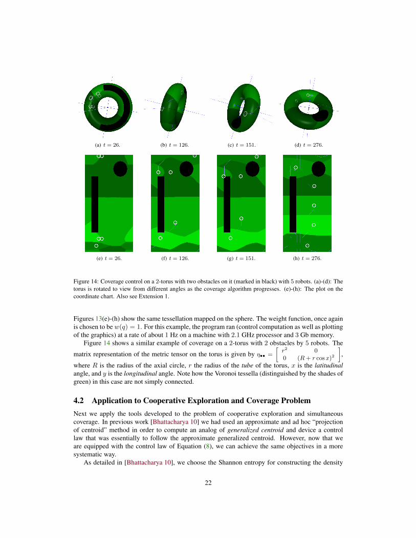
Figure 14: Coverage control on a 2-torus with two obstacles on it (marked in black) with 5 robots. (a)-(d): Thetorus is rotated to view from different angles as the coverage algorithm progresses. (e)-(h): The plot on thecoordinate chart. Also see Extension 1.

Figures 13(e)-(h) show the same tessellation mapped on the sphere. The weight function, once againis chosen to bew(q) = 1. For this example, the program ran (control computation as well as plottingof the graphics) at a rate of about 1 Hz on a machine with 2.1 GHz processor and 3 Gb memory.

Figure 14 shows a similar example of coverage on a 2-torus with 2 obstacles by 5 robots. The

matrix representation of the metric tensor on the torus is given by η•• =

[r2 00 (R+ r cosx)2

],

where R is the radius of the axial circle, r the radius of the tube of the torus, x is the latitudinalangle, and y is the longitudinal angle. Note how the Voronoi tessella (distinguished by the shades ofgreen) in this case are not simply connected.

4.2 Application to Cooperative Exploration and Coverage ProblemNext we apply the tools developed to the problem of cooperative exploration and simultaneouscoverage. In previous work [Bhattacharya 10] we had used an approximate and ad hoc “projectionof centroid” method in order to compute an analog of generalized centroid and device a controllaw that was essentially to follow the approximate generalized centroid. However, now that weare equipped with the control law of Equation (8), we can achieve the same objectives in a moresystematic way.

As detailed in [Bhattacharya 10], we choose the Shannon entropy for constructing the density

22

Region ofhigh Entropy

Splits area equally

Splits entropy equally

Sensor 1 Sensor 2

Figure 15: Entropy-weighted metric for voronoi tessellation in exploration problem.

function as well as to weigh the metric (Figure 15). Thus, if p(q) is the probability that the vertexq is inaccessible (i.e. occupied or part of an obstacle), for all q ∈ V(G), then the Shannon entropyis given by e(q) = − (p(q) ln(p(q)) + (1− p(q)) ln(1− p(q))). We use this for modeling thediscretized version of the weight function, w, and an isotropic metric, ζI (where I is the identitymatrix). Noting that in an exploration problem, the occupancy probability, p, and hence the entropye, will be functions of time as well, we use the following formulae for w and ζ,

w(q, t) =

εw, if e(q, t) < τe(q, t), otherwise. , ζ(q, t) =

εζ , if e(q, t) < τe(q, t), otherwise. (9)

for some small εw and εζ representing zero (for numerical stability).Each mobile robot maintains, updates and communicates a probability map for the discretized

environment and updates its entropy map. We use a sensor model similar to that describedin [Bhattacharya 10], and ‘freeze’ a vertex to prevent any change to its probability value when itsentropy drops below some τ ′ (< τ).

In addition, to avoid situations where a robot gets stuck at a local minima inside its tessellaeven when there are vertices with entropy greater than τ in the tessella (this can happen when thereare multiple high entropy regions in the tessella that exert equal and opposite pull on the robot sothat the net velocity becomes zero), we perform a check on the value of the integral of the weightfunction, w, within the tessella of the kth robot when its control velocity vanishes. If the integral isabove the value of

∫Vkεw dq, we switch to a greedy exploration mode where the kth robot essential

head directly towards the closest point that has entropy greater than the value of τ . This ensuresexploration of the entire environment (i.e. the entropy value for every accessible vertex drops belowτ ). And once that is achieved, both w and ζ become independent of time. Thus convergence isguaranteed.

Figure 16 shows screenshots of a team of 4 robots exploring a part of the 4th floor of the Levinebuilding at the University of Pennsylvania. The intensity of white represents the value of entropy.Thus in Figure 16(a) the robots start with absolutely no knowledge of the environment (maximumentropy), explore the environment, and finally converge to a configuration attaining coverage andminimum entropy (Figure 16(d)).

Figure 17 shows a similar scenario. However, in this case a human operator chooses to takecontrol of one of the robots (Robot 0, marked by red circle) soon after they start cooperative explo-ration of the environment. That robot is forced to stay inside the larger room at the bottom of theenvironment. Moreover, in this case we use a team of heterogeneous robots (robots with differentsensor footprint radii), thus requiring a power voronoi tessellation. This simple example illustratesthe flexibility of our framework with respect to incorporating human inputs to guide exploration.

23

(a) t = 2. (b) t = 300.

(c) t = 900. (d) t = 1550. Converged solution.

Figure 16: Exploration and coverage of an office environment by a team of 4 robots. Blue curves indicateboundaries of tessellation, intensity of white indicates the value of entropy. Also see Extension 1.

24

(a) t = 150. (b) t = 500.

(c) t = 1450. (d) t = 2100. Converged solution.

Figure 17: Exploration and coverage of an office environment discretized into a 284× 333 grid by a team of 4robots, with one of the robots (marked by red circle) being controlled by a human user. Also see Extension 1.

25

For either of the above examples, with the environment was discretized into a 284 × 333 grid,the program ran at a rate of about 3−4 Hz on a machine with 2.1 GHz processor and 3 Gb memory.

5 ConclusionIn this paper we have extended the coverage control algorithm proposed by Cortes, et al. [Cortes 04],to non-Euclidean configuration spaces that are, in general, non-convex. The key idea is the transfor-mation of the problem of computing gradients of distance functions to one of computing tangentsto geodesics. We have shown that this simplification allows us to implement our coverage controlalgorithm in any space after reducing it to a discrete graph. We have illustrated the algorithm byconsidering multiple robots achieving uniform coverage on a 2-sphere and an indoor environmentwith walls and obstacles. We have also shown the application of the basic ideas to the problem ofmulti-robot cooperative exploration of unknown or partially known environments.

AcknowledgementsWe gratefully acknowledge the support of the Office of Naval Research [grant numbers N00014-07-1-0829 and N00014-09-1-1031], the Army Research Laboratory [grant number W911NF-10-2-0016] and the Air Force Office of Scientific Research [grant number FA9550-10-1-0567].

Appendix: Proofs

Sketch of proof for Lemma L1:

Since Ω is a manifold with C1 boundaries, the ‘neighborhood’ of every p ∈ Ω will either resemblea complete Euclidean space (Figure 4(a)) or an Euclidean half space (Figure 4(b)). More technically, aλ-scaling of Ω at p will converge to RN or HN as λ → ∞, where N is the topological dimension of Ω(see Proposition 3.15 of [Gromov 99]). This indeed is a convex cone in Ti(p)RD (which, by definition, isλ-scaling of RD at i(p)). To prove that this space is TpΩ, we just invoke the local connectedness propertyof RN or HN , and hence existence of paths emanating from p that ‘fill’ the space.

Proof of Lemma L2:

An Ω that can be represented as a subset of a smooth, complete manifold of same dimension, alongwith the described path metric d`, is sometimes referred to as a metric space of type (∆) (see Theorem 2.1of [Wolter 85]).

i. The first result follows from the construction of the cut locus (see discussion in p. 42 of [Wolter 85]).

ii. The fact that gp is C1 in Ω − (∂Ω ∪ p ∪ Cp) follows from Theorem 3.1.b of [Wolter 85] (seeFigure 5(a)). In fact a stronger condition holds: The gradient of gp is locally Lipschitz continuous inΩ− (∂Ω ∪ p ∪ Cp) (by Theorem 5.1 of [Wolter 85]).

iii. If we choose q, q′ ∈ Ω − (∂Ω ∪ p ∪ Cp) at a distance of ε from each other, then due to the triangleinequality for the metric d`, we have |gp(q)− gp(q′)| ≤ ε. Thus it follows that the gradient of gp isbounded.

Sketch of proof for Lemma L3:

26

p

q

Ω

q

τ1

τ2q1

q2

(a) Illustration for Lemma L3, adapted from Figure 3.1 of[Wolter 85].

p

q

Ω

q

τ1

τ2q1

q2

Region of high curvature

(b) The same phenomenon can be created due to locallynon-Euclidean metric on manifold with boundary.

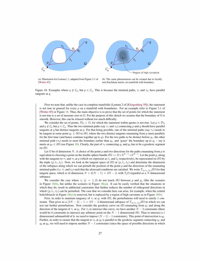
Figure 18: Examples where q /∈ Cp, but p ∈ Cq . This is because the minimal paths, τ1 and τ2, have paralleltangents at q.

First we note that, unlike the case in complete manifolds (Lemma 2 of [Klingenberg 59]), the statementis not true in general for every p on a manifold with boundaries. For an example refer to Figure 3.1 of[Wolter 85] or Figure 18. Thus, the main objective is to prove that the set of points for which the statementis not true is a set of measure zero in Ω. For the purpose of this sketch we assume that the boundary of Ω issmooth. However, this can be relaxed without too much difficulty.

We consider the set of points, DΩ ⊂ Ω, for which the statement within quotes is not true. Let p ∈ DΩ

and q /∈ Cp but p ∈ Cq . Thus the two minimal paths (say τ1 and τ2) connecting p and q should have paralleltangents at q but distinct tangents at p. For that being possible, one of the minimal paths (say τ1) needs tobe tangent at some point q1 ∈ ∂Ω to ∂Ω, where the two distinct tangents emanating from p meet parallelyfor the first time (and hence continue together up to q). For the two paths to be distinct before q1, the otherminimal path (τ2) needs to meet the boundary earlier than q1, and ‘graze’ the boundary up to q1 – say itmeets at q2 ∈ ∂Ω (see Figure 18). Clearly, the part of τ2 connecting q1 and q2 has to be a geodesic segmenton ∂Ω.

Let Ω be of dimension N . A choice of the point p and two directions for the paths emanating from p isequivalent to choosing a point on the double sphere bundle SΩ := Ω×SN−1×SN−1. Let the point p, alongwith the tangents to τ1 and τ2 at p (which we represent as t1 and t2 respectively), be represented on SΩ bythe triple (p, t1, t2). Now, we look at the tangent space of SΩ at (p, t1, t2) and determine the dimensionof the subspace along which we can perturb the position of the point p and the directions of the emanatingminimal paths (i.e. t1 and t2) such that the aforesaid conditions are satisfied. We write T(p,t1,t2)SΩ for thattangent space, which is of dimension N + 2(N − 1) = 3N − 2, with TpΩ regarded as a N -dimensionalsubspace.

We consider the case where τj (j = 1, 2) do not touch ∂Ω between p and qj (like the scenarioin Figure 18(b), but unlike the scenario in Figure 18(a)). It can be easily verified that the situations inwhich they do, result in additional constraints that further reduces the number of orthogonal directions inwhich (p, t1, t2) can be perturbed. The case that we consider here can arise, for example, when the centralhole/obstacle in Figure 18(a) is removed, but is replaced by a region of high curvature as in Figure 18(b).

First, in order to maintain tangency of τ1 at q1 with ∂Ω, the perturbations will need to satisfy 1 con-straint. That gives us a (3N − 2) − 1 = 3N − 3 dimensional subspace of T(p,t1,t2)SΩ in which we cantest our further perturbations. Now consider the geodesic curve on ∂Ω emanating from q1 and along thedirection of the tangent of τ1 at q1. For τ2 to intersect this curve, we have another N − 2 constraints (therewould be 0 constraints to intersect any arbitrary point on the N − 1 dimensional ∂Ω. Thus to intersect a 1dimensional submanifold of it, we need to impose (N −1)−1 constraints). This point of intersection is q2.Further, in order to ensure that the tangent to τ2 at q2 is parallel to the geodesic segment connecting q1 andq2 at q2, we will need to impose another N − 1 constraints (since the space of possible directions in which

27

it is possible to pass through q2 is SN−1, and we need τ2 to be tangent to a specific direction at q2). Thus, sofar, we have 1+(N−2)+(N−1) = 2N−2 constraints, that leaves us with a (3N−2)− (2N−2) = Ndimensional subspace of T(p,t1,t2)SΩ along which we can choose a direction to move (p, t1, t2) ans stillsatisfy the required conditions. Finally, we need to impose the constraint that the lengths of the paths τ1and τ2 need to be equal. This imposes 1 additional constraint. Thus, the dimensionality of the subspace ofT(p,t1,t2)SΩ along which we can perturb the point p and the emanating directions of τ1 and τ2 is N − 1.Even if this subspace lies entirely in TpΩ ⊂ T(p,t1,t2)SΩ, it is one dimension less than the dimensionalityof TpΩ. Thus the dimensionality of DΩ can at most be N − 1.

As discussed earlier, we first prove Lemma L4 and Corollary C1, using which we will prove theProposition P1.

It is possible to prove Lemma L4 using more direct arguments that establish the direction ofsteepest descent of a function in the tangent space as the dual of the differential of the function (i.e.gradient of a function). However, for completeness, we provide an explicit proof.

Proof of Lemma L4:

For notational convenience, let us define gw(u) := dC(w,u), ∀u ∈ Img(φ). Recall that geodesicallyconvex implies that any two points in U can be connected using a smooth geodesic segment (a curvesatisfying the geodesic equation at every point) lying entirely in U .

Consider gw as a function from RD to R+ with an unique minima at w. Let γwq represents anyarbitrary curve in Img(φ) ⊆ RD connecting w to q. By the fundamental theorem of calculus and using thefact that gw(w) = 0, we have,

I(γwq) := gw(q) =

∫γwq

∂

∂ugw(u) · du ≡

∫γwq

∂gw(u)

∂uidui (10)

where, [ du1, du2, · · · , duD] is the coefficient vector (in chart C) of an infinitesimal element along thetangent to the curve.

Now, the length of the curve γwq is given by

L(γwq) :=

∫γwq

√ηij(u) dui duj (11)

By definition, the value of L(γwq) is minimum when γwq is the shortest geodesic (which, due to thehypothesis that the cut locus of any point in U is empty, is unique – call it γ∗wq) connecting w and q, andthe minimum value is clearly gw(q) (by definition of gw). Thus,

L(γwq) ≥ I(γwq) [= gw(q), a const. independent of γwq] ,equality holds when γwq = γ∗wq

(12)

Now, consider a family of infinitesimal elements of RD represented by the coefficient vector du =[ du1, du2, · · · , duD]T located at an arbitrary point u ∈ Img(φ) such that u + du lies inside Img(φ).From the triangle inequality of dC (since it is induced by a Riemannian metric) we have,

dC(w,u + du) ≤ dC(w,u) + dC(u,u + du)

=⇒ dC(w,u + du)− dC(w,u) ≤ dC(u,u + du)

=⇒ ∂

∂ugw(u)

∣∣∣∣u

· du ≤√ηij(u) dui duj

=⇒ ∂gw(u)

∂uidui ≤

√ηij(u) dui duj =

ηij(u) dui duj√ηmn(u) dum dun

(13)

28

Equality of the triangle inequality in (13) of course holds when u lies on the geodesic connecting w andu + du.

Now consider a curve γ′wq (connecting w and q) with infinitesimal elements du along the tangents tothe curve. If there exists at least one point along that curve on which the inequality in (13) is not an equality,then the integrals of the quantities on the two sides of the inequality will not be equal. That is, for such acurve we will have I(γ′wq) < L(γ′wq).

But we know that there does exist a curve, γ∗wq, such that I(γ∗wq) = L(γ∗wq) does hold. Thus, for thatcurve it should be true that at each and every point of the curve the equality of (13) holds true. Thus wehave essentially shown that for the geodesic, γ∗wq, at each and every point of the curve the following holds

∂gw(u)

∂uidui =

ηij(u) dui duj√ηmn(u) dum dun

where du are of course infinitesimal elements at u along the tangent to γ∗wq.One can normalize by dividing by ‖ du‖2 to obtain

∂gw(u)

∂uiziqu =

ηij(u)ziquzjqu√

ηmn(u) zmquznqu(14)

where ziqu is the ith component of the tangent vector at u to the geodesic connecting w to u, which due toour assumption is unique. We note that the right-hand-side of the above equation represents a scalar field(call it S). Also, ziqu (which are functions of u) represent the coefficients of a contravariant vector field in(U −w). Thus, writing Xi for ∂gw(u)

∂ui, one can rewrite Equation (14) as

Xiziqu = S(u) (15)

where we need to solve for the coefficients Xi(u) := ∂g(u)∂ui

. Of course a particular solution is

X0,i(u) =ηij(u)zjqu√ηmn(u) zmquznqu

(16)

These coefficients clearly transform as coefficients of a covariant vector field. Moreover, the contravariantvector field corresponding to this covariant field (i.e. the vectors with coefficients X0,i = ηijX0,j) isparallel to ziqu. From this we can infer that the solution mentioned in (16) is the only solution of (15)that transforms as coefficients of a covariant vector field (This is because of the following: Every covarianttransformation of Xi corresponds to an unique contravariant transformation of Xi. Again, the generalsolutions of Xi need to be such that ηijziquXj = ηijz

iquX

0,j = βηijziquz

jqu for some scalar field β. This

needs to be true in every coordinate chart. Due to positive definiteness of η••, this is possible only with Xj

parallel to zjqu, which also fixes the scalar multiple β since we have the known scalar field, S. ).Thus we have

∂gw(u)

∂ui=

ηij(u)zjqu√ηmn(u) zmquznqu

(17)

Thus, by specializing for u = q, we obtain the proposed result.

Proof of Corollary C1:

We first note that due to Lemma L2, we can always choose an open neighborhood of q, Bq ⊆ V , whichis geodesically convex, on which the function gp := d`(p, ·) is of class C1, and the cut locus of every pointin which is empty in Bq (since q /∈ Cq).

Consider a minimal path γ∗pq connecting p and q. Let w(6= q) be a point on this path (between p and q)that lies inside Bq (which we can always find since Bq is open) – see Figure 8(a).

29

From the definition of minimal path we have γ∗pq = γ∗pw ∪ γ∗wq , for a minimal path, γ∗pw, connecting pand w, and the minimal geodesic, γ∗wq , connecting w and q (which is unique since q /∈ Cp). Thus it followsthat,

zpq = zwq (18)

Again, by triangle inequality, for any u ∈ ψ(Bq)

dD` (p,u) ≤ d`(p, w) + dD` (w,u)

⇒ gp(u) ≤ h(u) (19)

where h(u) := d`(p, w) + dD` (w,u) and gp(u) := dD` (p,u).However, equality does hold when p, w and ψ−1(u) lie on the same shortest path. This, in particular, istrue when u = q (due to our choice of w). Now, since q /∈ Cp and by our choice of Bq , both gp and h areof class C1 at q. Thus we have gp(u) ≤ h(u) for u ∈ ψ(Bq), and at u = q they satisfy equality and aredifferentiable. This implies the differentials of the functions at q should be same,

∂

∂ugp(u)

∣∣∣∣u=q

=∂

∂uh(u)

∣∣∣∣u=q

⇒ ∂

∂udD` (p,u)

∣∣∣∣u=q

=∂

∂udD` (w,u)

∣∣∣∣u=q

(20)

Now, Bq satisfies the conditions for U in Lemma L4, and w and q are points inside it. Thus byLemma L4,

∂

∂uidD` (w,u)

∣∣∣∣u=q

≡ ∂

∂uidD` (w,u)

∣∣∣∣u=q

=ηij(q) zjwq√ηmn(q) zmwqznwq

(21)

where w = ψ(w).Substituting from (18) and (20) into (21) we obtain the proposed result.

Proof of Proposition P1:

Equipped with Corollary C1 we can now conclude the proof of Proposition P1. The gradient of afunction is, by definition, the dual of the differential, i.e. grad(f) =

(∂f∂xi

dxi)∗

= ηij ∂f∂xj

∂∂xi

. Let q be apoint on ∂Ω and qi be a Cauchy sequence of points converging to q. Due to Corollary C1, at every pointqi ∈ Ω− (∂Ω∪ p∪Cp), the negative of the gradient of the distance from p is parallel to−zpqi , the tangentat qi to the minimal path connecting qi to p (Figure 6). Due to our definition of gradient at boundary points,the gradient of the distance function at q will then be limi→∞−zpqi . Since d` is a path metric, the minimalpath connecting each qi to p exists in Ω, as does the path connecting q to p. Thus, the limit exists in TqΩ.

References[Alexander 81] S. Alexander. Distance geometry in Riemannian manifolds-with-boundary.

vol. 838, pages 12–18, 1981.

[Bhattacharya 10] S. Bhattacharya, N. Michael & V. Kumar. Distributed coverage and explo-ration in unknown nonconvex environments. In Proceedings of the 10th Interna-tional Symposium on Distributed Autonomous Robotics Systems, pages 1–14.Springer, 2010.

30

[Bullo 09] F. Bullo, J. Cortes & S. Martınez. Distributed control of robotic networks: Amathematical approach to motion coordination algorithms. Applied MathematicsSeries. Princeton University Press, 2009.

[Cormen 01] Thomas H. Cormen, Clifford Stein, Ronald L. Rivest & Charles E. Leiserson.Introduction to algorithms. McGraw-Hill Higher Education, 2001.

[Cortes 04] J. Cortes, S. Martinez, T. Karatas & F. Bullo. Coverage control for mobile sens-ing networks. IEEE Trans. Robot. Autom., vol. 20, no. 2, pages 243–255, April2004.

[Cortez 04] Jorge Cortez, Sonia Martinez, Timur Karatas & Francesco Bullo. Coverage Con-trol for Mobile Sensing Networks. IEEE Trans. Robot. and Automat., vol. 20,no. 2, pages 243–255, 2004.

[Cortez 05] Jorge Cortez, S. Martinez & Francesco Bullo. Spatially-distributed coverageoptimization and control with limited-range interactions. ESIAM: Control, Op-timisation and Calculus of Variations, vol. 11, pages 691–719, 2005.

[Cundy 89] H. Cundy & A. Rollett. Mathematical models. Tarquin Pub., 3rd edition, 1989.

[Dijkstra 59] Edsger W. Dijkstra. A note on two problems in connexion with graphs. Nu-merische Mathematik, vol. 1, pages 269–271, 1959.

[Durham 12] J.W. Durham, R. Carli, P. Frasca & F. Bullo. Discrete Partitioning and CoverageControl for Gossiping Robots. IEEE Transactions on Robotics, vol. 28, no. 2,pages 364–378, 2012.

[Gromov 99] M. Gromov, J. Lafontaine & P. Pansu. Metric structures for riemannian andnon-riemannian spaces. Progress in mathematics. Birkhauser, 1999.

[Jost 97] J. Jost. Compact riemann surfaces. Springer-Verlag, 1997.

[Klingenberg 59] W. Klingenberg. Contributions to Riemannian Geometry in the Large. Annalsof Mathematics, vol. 69, no. 3, pages 654–666, May 1959.

[Lloyd 82] Stuart P. Lloyd. Least squares quantization in PCM. IEEE Trans. Inf. Theory,vol. 28, pages 129–137, 1982.

[Lozano-Perez 79] Tomas Lozano-Perez & Michael A. Wesley. An algorithm for planningcollision-free paths among polyhedral obstacles. Commun. ACM, vol. 22,no. 10, pages 560–570, October 1979.

[Munkres 99] James Munkres. Topology. Prentice Hall, 1999.

[Petersen 06] P. Petersen. Riemannian geometry. Graduate Texts in Mathematics. Springer,2006.

[Pimenta 08] L. C. A. Pimenta, V. Kumar, R. C. Mesquita & G. A. S. Pereira. Sensing andCoverage for a Network of Heterogeneous Robots. In Proc. of the IEEE Conf.on Decision and Control, pages 3947–3952, Cancun, Mexico, December 2008.

31

[Rimon 92] E. Rimon & D.E. Koditschek. Exact Robot Navigation Using Artificial PotentialFields. IEEE Transactions on Robotics and Automation, vol. 8, no. 5, pages501–518, 1992.

[Sastry 99] S. Sastry. Nonlinear systems: Analysis, stability and control. Interdisciplinaryapplied mathematics: Systems and control. Springer, 1999.

[Stachniss 05] C. Stachniss, G. Grisetti & W. Burgard. Information Gain-based ExplorationUsing Rao-Blackwellized Particle Filters. In Proc. of Robot.: Sci. and Syst.,pages 65–72, Cambridge, MA, June 2005.

[Stachniss 06] C. Stachniss. Exploration and Mapping with Mobile Robots. PhD thesis, Uni-versity of Freiburg, Freiburg, Germany, April 2006.

[Thrun 05] Sebastian Thrun, Wolfram Burgard & Dieter Fox. Probabilistic robotics (intelli-gent robotics and autonomous agents). The MIT Press, 2005.

[Wolter 85] Franz-Erich Wolter. Cut loci in bordered and unbordered Riemannian manfolds.PhD thesis, Department of Mathematics, Technical University of Berlin, 1985.

32