Multi-Period VaR-Constrained Portfolio Optimization with

Multi-Period VaR-Constrained Portfolio Optimization with Applications to the Electric Power Sector

Paul R. Kleindorfer* The Wharton School/OPIM University of Pennsylvania

Philadelphia, PA 19104-6340 [email protected]

and

Lide Li

PowerTeam, Exelon Corporation, 300 Exelon Way

Kennett Square, PA, 19348 [email protected]

May 2004

Abstract This paper considers the optimization of portfolios of real and contractual assets, including derivative instruments, subject to a Value-at-Risk (VaR) constraint, with special emphasis on applications in electric power. The focus is on translating VaR definitions for a longer period of time, say a year, to decisions on shorter periods of time, say a week or a month. Thus, if a VaR constraint is imposed on annual cash flows from a portfolio, translating this annual VaR constraint into appropriate risk management/VaR constraints for daily, weekly or monthly trades within the year must be accomplished. The paper first characterizes the multi-period VaR-constrained portfolio problem in the form Max {E – kV} subject to a set of separable constraints over the decision variables (the level of assets of different instruments contained in the portfolio), where E and V are, respectively, the expected value and variance of multi-period cashflows from operations covered by the portfolio. Then, assuming the distribution of multi-period cashflows satisfies a certain regularity condition (which is a generalization of the standard Gaussian assumption underlying VaR), we derive computationally efficient methods for solving this problem that take the form of the standard quadratic programming formulations well-known in financial portfolio analysis.

* Corresponding author

1

Multi-Period VaR-Constrained Portfolio Optimization with Applications to the Electric Power Sector1

1. Introduction Fueled in part by the rapid growth of electronic exchanges for a number of services and commodities, the problem of optimization of portfolios of forward and derivative instruments, and related real (physical) options has become an important area of application in computational finance. As reviewed in Kleindorfer and Wu (2003), this problem is now an important ingredient of coordinating supply and demand, and of associated financial hedging, in applications as diverse as currency risk management, insurance, chemicals, transportation (e-logistics), and energy. The typical problem involves the trading operations of a company that has opportunities to contract with customers and suppliers to structure forward and options contracts to buy or sell contingent obligations, with financial or physical settlement, where such obligations/contracts are typically benchmarked on an underlying spot market for the commodity in question or for a close substitute. The company can meet and hedge its contingent obligations through a variety of means based on short-term and long-term contracts executed directly with other agents in the marketplace. The company can also build or contract for physical capacity to meet or hedge its contractual obligations. A central problem in this context is the optimization of portfolios of such real and contractual assets, subject to a Value-at-Risk (VaR) constraint. While definitions of VaR vary across applications, the standard definition of the VaR of a portfolio is the maximum loss that the portfolio is allowed to sustain over a specified period of time and at a specified level of probability.2 VaR constraints are imposed in order to limit the maximum loss that responsible decision makers feel they can prudently sustain from a portfolio of assets and contracts over a defined period of time. Our focus in this paper is on characterizing multi-period VaR-constrained portfolio optimization. We focus on the impact of multi-period risk constraints covering a period such as a year or a quarter on decisions affecting cash flows during shorter periods of time, say a week or a month. This problem is important in energy management since accounting periods, which are useful control points for investors and markets, are typically longer than the operational periods over which trading decisions must be taken. Thus, if a VaR constraint is imposed on annual cashflows from a portfolio, translating this annual VaR constraint into appropriate risk management/VaR constraints for daily, weekly or monthly trades within the year must be accomplished in one or another manner, since at least some

1 The authors gratefully acknowledge helpful comments on this paper by Andrew Huemmler,Vincent

Kaminski, Shmuel Oren, Weiya Pang, and Al Roark. Anonymous reviewers also contributed significant improvements to the paper. Remaining errors are our own.

2 See, e.g., Marshall and Siegel (1997) and Crouhy, Galai and Mark (2000). We note right away that while VaR is the most widely used risk measure, it is not universally accepted, with “expected shortfall” being an alternative measure of risk espoused by several researchers. Perhaps the primary advantage of VaR is that it is readily understandable by risk managers. See Artzner et al. (1999, 2002) and Rockafellar and Uryasev (2000) for a detailed discussion of the theory and computation of risk measures, including applications to multi-period risk assessment.

2

contingent obligations represented in the portfolio will be realized over shorter periods than a year. Our particular focus will be on electricity trading, an arena in which the portfolio optimization problem is clearly important. (Clewlow and Strickland, 2000; Kamat and Oren, 2002; Mount, 2002; Banerjee and Noe, 2002; Bessembinder and Lemmon, 2002; Eydeland and Wolyniec, 2003) Electric power is especially interesting as an application area for portfolio optimization.3 In the restructured electricity market, producing Sellers (Generators) and Buyers (Load Serving Entities and Distribution Companies) can sign bilateral contracts to cover the demands of their retail and wholesale customers. These bilateral contracts may cover purchases/sales for up to a few years in advance. They can also interact through the spot market on the day. Finally, Sellers and Buyers can buy hedge instruments whose payouts are correlated with both the prices of bilateral contracts as well as with the underlying spot market. How much of their respective capacity and demand Sellers and Buyers should or will contract for in the bilateral contracting market and spot markets, how much generation they should own to cover their obligations, and the appropriate hedging of their positions through financial instruments are the basic decisions underlying the portfolio optimization problem of interest. Interestingly, while some aspects of this problem, e.g. the valuation of various derivative instruments, enjoy a considerable literature, the analysis of the VaR-constrained multi-period portfolio problem has not been analyzed previously in the extensive literature on energy trading and supply-management strategies.4 Rather, only stylized single-period portfolio models, with all contingent claims maturing at the same end date, have been the standard for both theory and practice, e.g. Marshall and Siegel (1997); Coronado (2000). These build on a very illustrious history of financial portfolio analysis going back to the 1950s (Markowitz, 1952; Sharpe, 2000; Brealey and Myers, 1991). We will show that there are important problems and implications associated with a more detailed multi-period analysis of the VaR-constrained portfolio optimization problem that are essentially hidden in the single-period models analyzed to date. A central assumption underlying most VaR computations is that of normality. While this has considerable appeal and justification in financial markets, it is generally recognized that energy markets, and especially electric power markets, experience short-term price spikes that give rise to “fatter tails”, even in annual cash flow distributions, than are compatible with normality. The analysis below provides a more general treatment of VaR that captures the case of normality but also other cases such as Student-T, Weibull and many other distributions. The needed assumption for our analysis is that the left-tail of the distribution of multi-period cash flows, denoted Π, be representable in the form ),,( γσµh , with

),,( γσµh defined by γγσµµΠ −=−≤ 1)},,(hPr{ , with µ and σ denoting, respectively,

3 For an introduction to the extensive literature on risk management in electric power, see the recent overview by EIA (2002) and the applications in Woo et al. (2003, 2004). 4 But see Humphreys and McClain (1998) and Mount (2002) for predecessors of this analysis of portfolios in environments without VaR constraints. For an application of dynamic hedging to agricultural commodities, wee Haigh and Holt (2002).

3

the mean and standard deviation of Π. This assumption is clearly satisfied if Π is normally distributed, with h defined as σγγσµ )(),,( Zh = , where Z(γ) is the normal z-score for γ. While the electricity sector is similar in many respects to other commodity trading sectors, there are also some special characteristics in this sector that influence the nature of trading and portfolio optimization. A key and well-known differentiating factor is that electric power can be stored economically only in very limited quantities (e.g., via pumped storage, which is not very efficient). This gives rise to a much more volatile and weather-driven spot price. Other essential elements of energy portfolio management that are captured in the analysis that follows include:

1. The elements of the portfolio, to be optimized, include fixed generation assets owned or leased by the company (which may be changed through merger & acquisition activity or sale of assets), long-term power purchase agreements (PPAs) signed by the company, and various types of forwards, puts and calls for financial and physical settlements that are benchmarked on the underlying spot market.

2. The company of interest may also have retail customers whose rates are regulated, giving rise to special risks in that these customers typically have an unlimited floating-volume call option on the company’s supply portfolio at the fixed, regulated price.5

3. Buying and selling of generation assets can take place at fixed decision points any time within the planning horizon, which we will refer to as a “year”. Forward and option trades are executed at various points during the year and may cover different intervals of time (weeks, months, quarters, …).

4. Fixing a specific time period, e.g., a year, the typical VaR constraint has the following structure:6

Pr{DCF + ∆DNV – C – rK > -VaR0} = γ (1)

where VaR0 > 0 is the magnitude of the allowed Value-at-Risk, DCF is the value of discounted cash flows arising from the trading portfolio over the year, ∆DNV is the NPV of the change in valuation for open positions at the end of the year compared to

5 The California experience provides a sobering example of what happens when these risks are neglected.

While there were many problems in California, neglecting the risks of capped retailed prices in the face of volatile and increasing wholesale prices was certainly a key factor in the difficulties that ensued for California distribution companies. See Sweeney (2002) for a discussion of the causes and consequences of the California debacle. One of the consequences of this has been the need, indeed the requirement according to the California Assembly Bill AB57 (2002), for detailed risk assessment of energy procurement contracts for California’s distribution companies going forward. The most recent electric power failure, transmission-related, in Northeastern United States and Canada, on August 14, 2003, has further heightened interest in risk management and portfolio optimization.

6 We will provide a much more detailed exposition of the structure of the VaR constraint and cashflows for a general portfolio of electric power options in the model below.

4

the beginning of the year, C is the NPV of any expenses for trading and managing the portfolio, not captured in DCF, and rK are any required annualized payments to investors for capital invested in the portfolio (e.g., for capital invested in owned generation). The risk parameter γ (e.g., 0.95) represents the required probability associated with the “risk appetite” of the company in defining its VaR. Constraints on minimum cashflows generated by a portfolio to cover specific forms of debt, fixed investor payouts, or other management objectives, can be incorporated in C in the above definition.

The primary question addressed here is: How does one represent a multi-period, e.g. an annual, VaR-constraint of the above form in terms of constraints on lower levels of temporal aggregation to cover instrument choices made during the course of the year. To illustrate the problem, consider the following approach, which might be called equally weighted or uniform disaggregation. This approach would take the annual VaR as given above, and apply it equally to sub-intervals of the year. Thus, the VaR for a typical week would be taken to be VaR/52, for a typical day VaR/365, and so forth, always utilizing the same risk parameter γ. This approach is not very clever, since (among other problems) it does not even treat the multi-period pooling effect of daily decisions. To capture the pooling effect, assume that annual cashflows Y from the portfolio are the sum of 365 daily cashflows and that each of these daily cashflows is normally distributed with mean µd and standard deviation σd. Then, assuming daily cash flows are stochastically independent, denoting the typical daily cashflow as Xt, and neglecting discounting, it follows that

∑=

−≥===−≥365

1tatdt }VaRXYPr{}VaRXPr{ γ (2)

provided that the daily VaR (VaRd) and annual VaR (VaRa) are defined as

VaRd = z(γ)σd - µd; VaRa = z(γ)σa - µa (3) with

365;

365a

da

dµ

µσ

σ == (4)

where )(γz is the z-score of a standardized normal random variable, e.g. z(0.95)=1.65. It is clear that if the VaR rule on the l.h.s. of (2) is implemented on a daily basis, then the annual VaR constraint on the r.h.s. of (2) will be satisfied. However, even this more clever approach is not very satisfying, afflicted as it is with strong assumptions about normal, independent and identical distributions and with no optimization of the cashflows involved. Moving beyond these simple notions of VaR disaggregation in an optimizing framework is the main objective of this paper. We proceed as follows. The next section provides a statement of the general VaR-constrained portfolio optimization problem of interest and characterizes the efficient frontier

5

for such problems as an optimization problem with separable constraints across the instruments that are the subject of the optimization. Section 3 then applies these results in the electric power context, and provides an efficient computational algorithm in the case where period cash flows may be assumed to be statistically independent. We discuss the non-independent case as an extension. Section 4 provides some illustrative examples of the method proposed, including a brief discussion of the use of existing spot price data management and simulation systems to obtain the distributions and statistics needed for the approach suggested. Section 5 is by way of conclusion. 2: Efficiency for VaR-Constrained Portfolios This section is concerned with characterizing the efficient frontier for VaR-constrained, expected profit-maximizing optimal portfolios. The efficient frontier in Expected Profit and VaR space (referred to for short as E-VaR space) is the set of Expected Profit, VaR pairs achievable from feasible portfolios such that there is no other feasible portfolio producing the same or higher Expected Profit at a lower VaR. This section characterizes the efficient frontier in E-VaR space in a manner that is convenient for computation when instruments in the portfolio may have shorter duration contractual terms than the overall planning horizon. We proceed in this section quite generally, becoming more specific in the next section in the application of these results to electric power. Throughout this discussion, the reader may think of the instruments referred to as calls, puts, forwards, and (cashflows from) owned generation for a specific firm, referred to as the Company, involved in either retail or wholesale operations in electric power. Let Π = profits/cashflows, including payments for all instruments used; in the case where some of the assets in the portfolio are capitalized (e.g., owned generation), profits may also include payments to capital owners on an appropriate (e.g., annualized) per period basis.7 Let N = number of periods in the planning horizon T for the portfolio optimization problem. The reader might think of T as a year with N (monthly or quarterly) sub-periods, during which instruments may be traded. The usual approach to VaR relies on normality. If the sub-periods are sufficiently numerous, and the correlation structure between periods is simple, e.g., only successive periods are correlated with one another, then N-period profits, the sum of the individual subperiod profits, could be assumed to be normally distributed by the Central Limit Theorem.8 However, since spot price distributions and spot demands may exhibit spiking and “regime switching” behavior (Ethier and Mount, 1998), it is possible that the distributions of cash flows may have fatter tails than the normal distribution, except when N is very large. To capture this possibility, we will relax the normality assumption to

7 There are several notions of VaR possible, depending on what aspect of cash flows are earmarked for the

VaR definition. For example, these might simply represent trading cashflows. Or they might represent more generally EBIT from the Company’s generation SBU, or they might represent cash flows, net of certain specified capital allocations for the Company. While these are important managerial distinctions, which would influence the definition of C in (1) and therefore the definition of VaR, they would not affect the theoretical development below in any substantial way.

8 See Hull and White (1998) for an early discussion of the normality assumption underlying VaR.

6

accommodate other distributions that exhibit fat-tail characteristics. We assume the following regularity assumption (RA) on the left-tail of the distribution of Π.9 RA: Let Π be a random variable (representing multi-period cashflows) whose probability distribution function is continuous with meanµ and standard deviation σ . Let γ be the confidence level of the VaR constraint, 0<γ <1. Then, for any specified ),,( γσµ , there is a real number ),,( γσµh such that γγσµµΠ −=−≤ 1)],,(hPr[ , where h is continuous in its arguments and strictly increasing inσ , and where h(µ, σ, γ) - µ = VaR(µ, σ, γ ) is non-increasing in µ. If Π is normally distributed, then RA is satisfied with σγγσµ )(),,( Zh = , where Z(γ) is the standard z-score. Other well-known distributions such as student-T and Weibull (for any fixed shape) can be described in this way. The assumptions embodied in RA that the VaR of a portfolio should be increasing in σ and decreasing (or at least non-increasing) in µ are motivated by similar generalizations of the traditional portfolio problem under normality to the more general mean-variance efficient-frontier tradeoff analysis (Sharpe, 2000). If RA is satisfied for the cashflows Π from a portfolio, then the portfolio’s VaR is

)()),(),((h)(VaR ΠµγΠσΠµΠ −= (5)

We denote by Q the vector of possible instruments (puts, calls, forwards, etc.) that might be included in various portfolios. Similarly, denote by Dt the random variable for demand in time period t, Pt the random variable for spot price in time period t. Let VaR0 be the desired annual constrained VaR level at confidence level γ. Finally, denote by )P,D,Q(Π the annual cashflows resulting from Q, D, P, with µ(Q,D,P) and σ(Q, D, P) the mean and standard deviation of )P,D,Q(Π . With these assumptions and notation, we can state the N-period, VaR-constrained problem of interest as follows:

)P,D,Q(})P,D,Q({E)}P,D,Q({EMaximizeN

tttt µΠΠ == ∑

=1 (6)

Subject to: )),P,D,Q(),P,D,Q((hVaR)}P,D,Q({EN

tttt γσµΠ∑ ≥+

=10 (7)

where 50

1

.

tttN

t)P,D,Q(VAR)P,D,Q(

= ∑

=Πσ (8)

9 We analyze in Kleindorfer and Li (2004), available from the authors on request, a number of scenarios, using both simulated and real data (from PJM) to determine whether RA is a reasonable assumption for real power data, as prices and loads exhibit significant spikes and other anomalies. We show in Kleindorfer and Li (2004) that even a small number of instruments (4) and periods (4) serve to smooth out the distribution of cashflows sufficiently to allow RA to be calibrated. We also show for these problems that normality is not a good assumption even though RA is satisfied.

7

The correlation structure of cashflows generated by portfolio instruments between various periods in the planning horizon is captured in σ(Q, D, P). Denoting by E = µ(Q,D,P), the expected value of the profit function over these random variables, we can re-state the problem (6)-(8) in abbreviated form as

Maximize E (9) Subject to: ),,E(hVaRE γσ≥+ 0

Let us first proceed somewhat heuristically. We dualize the constraint in (9) using the Lagrange multiplier 0≥λ to obtain the Lagrangean: )),,(()1(),,( 0 γσλλλσ EhVaREE −++=Λ (10) Dividing by (1+λ) and defining k = λ/ (1+λ), and noting that VaR0 is a constant, we can use the Karush-Kuhn-Tucker (KKT) conditions to characterize (heuristically for the moment) the solution to problem (9) as: Maximize ),,E(hkE γσ− (11) While it is not intuitively obvious, we show below that the set of {E(k), σ(k) | k > 0} solving (11) as k varies (the efficient frontier in (E, σ) space) can actually be obtained by solving for the efficient frontier in E-V space, where V = σ2, i.e. by solving the following problem for varying k: Maximize 2σkE − = E – kV (12) where the maximization in (12) is w.r.t. feasible instruments Q. As the constraints on individual instruments are generally separable across instruments (e.g., entailing just lower and upper bounds on total purchases or sales of a specific instrument), this problem has a very simple (separable) constraint structure, even when demands, prices and cashflows are serially correlated across sub-periods. The reader can retrace the above heuristic argument leading to (11) to note that it actually holds quite generally when the KKT conditions are necessary and sufficient. However, rather than becoming embroiled in a technical analysis of the KKT conditions, including interior versus boundary solution conditions, and issues related to overlapping and non-overlapping instruments, we will show directly that the procedure just presented is valid in general, and leads to a mathematical programming problem with a separable constraint set that can be solved by a variety of methods. The next two claims, proved in the Appendix, establish the necessary foundation for our approach. Claim 1. Assume that aggregate cashflows satisfy RA. For fixed k > 0, let Q = Q(k) be the portfolio obtained by maximizing E - kV. Then, as shown in Figure 1, Q(k) is on the left

8

c

ckVE +=

Q(k) Q(k)

border of the feasible set in E-V space; it is also on the left border of the feasible set in E-σ, and E-VaR space (i.e., if Q’ is any other feasible portfolio for which E(Q’) = E(Q(k)), then VAR(Q’) > VAR(Q), VaR(Q’) > VaR(Q) and σ(Q’) > σ(Q)). There may be multiple portfolios yielding the same expected profit and standard deviation. We may think of these for the purposes of the present VaR analysis as an equivalence class, as any of these will do equally well from the point of view of efficiency in E-VaR space. Claim 2. Assume that aggregate cashflows Π satisfy RA. Then, if Q is any portfolio on the efficient frontier in E-VaR space, there is a k > 0 such that Q is a solution to maximizing E - kV. Claim 2 implies that we can generate the efficient frontier in E-VaR space by varying k and maximizing E-kV (subject to whatever constraints might be imposed on the available individual instruments). For those assets in the portfolio that generate cash flows only during specific sub-periods, the determination of their optimal levels through the problem Max(E -kV) is relatively straightforward as it concerns only those periods in which cashflows are affected. Since constraints on the instruments are typically separable and apply only to those instruments, simple search procedures can be applied to this problem even under very general conditions. In many applications this allows a computable solution to the multi-period problem of interest. We illustrate this below for the power sector. Before continuing, it is important to note that the efficient frontier we obtain here is the solution for the “Open Loop Problem”, which determines expected uses of instruments over an ensuing planning horizon. Our assumption in the above algorithm is that the portfolio, once selected, will not be changed during the period in discussion. In practice, a rolling horizon approach would be used in which the problem of interest would be resolved, say every month, with updated information. The next month’s results would be implemented, based on the proposed open loop methodology. At the end of the month, demand and price data, and available instruments, would be updated and the problem resolved. Note that an efficient algorithm to solve the “Dynamic Closed Loop Problem” would assume two types of updating: First, there would be embedded in the underlying dynamic model the evolution of information on market conditions (price and demand) and the choice of sub-period instruments would, in fact, be state dependent. Second, the amount of the annual VaR

V

E

Figure 1 Figure 2

E

σ

9

constraint actually “consumed” through sub-period t would be noted and could also condition the riskiness of positions from period t forward. In the application area of interest here, electric power, neither of these types of updating is compelling. Regarding the first, one knows just about as much about the month of July, say, at the beginning of the year as one does at the beginning of June, when updated market conditions might yield state-contingent alterations in one’s portfolio. Regarding the second issue, companies engaged in electric power trading treat trading on a “going firm” basis, so that the annual VaR constraint for the year beginning, say, in January is typically the same as the annual VaR constraint for the year beginning in June or July, and this irrespective of the particular performance of trading operations through May or June. Of course, VaR controls do change as managerial judgment and market conditions change, but Open-Loop approximations, under a rolling horizon assumption, are a reasonable point of departure for planning.10 We return to the implementation issues below, after discussing the electric power sector in more detail. 3. Structure of the Optimal Portfolio for the Electricity Sector This section builds on the theory of the preceding section in providing a general model for portfolio optimization involving familiar instruments used in electric power portfolios. We imagine an integrated utility, called the “Company”, that may own or lease generation, that has a trading division that can sign contracts for Power Purchase Agreements (PPAs), as well as puts, calls and forwards based on an underlying wholesale spot market. We abstract here from transmission constraints or markets.11 We also imagine that the Company has some retail operations that are regulated, and that the Company is a price-taker in the wholesale market and cannot affect the price of any traded derivative.12 We will take the simplest possible approach to the regulated sector, assuming a fixed, exogenously determined regulated price per KWh, independent of time. More complicated regulatory scenarios are easily incorporated into the framework developed. Note the critical difference between competitive wholesale spot transactions and regulated retail transactions for the Company. Instruments sold in the wholesale market will be typically rather specific as to temporal and capacity restrictions. Retail transactions, on the other hand, are load-following. In effect, retail customers have a capacity-unlimited call option on the Company, which must either be fulfilled from the Company’s portfolio of generation, PPAs and options/forwards, or from the spot market at the prevailing wholesale price at the time the retail customer makes his demand.13 It is this feature of customer

10 For a more general discussion of open-loop, rolling horizon approximations to closed-loop control problems,

see Bertsekes (1995) and Morari and Lee (1999). 11 To the extent that these are based on principles of Locational Marginal Prices (LMP), as in the PJM market,

transmission constraints and options could also be included as part of the portfolio optimization described below.

12 The model developed below applies equally to trading and wholesale power brokers, whether or not they have retail sector commitments at regulated prices. For a review of competitive derivative markets, involving the types of real options discussed here, see Kleindorfer and Wu (2003).

13 For a good discussion and formal modeling of the consequences from the risks arising from fixed retail prices faced by power distribution companies, see Banerjee and Noe (2002).

10

demand at regulated prices, together with the weather-driven level of spot prices and the non-storability of electric power, that makes electricity supply a risky business. We are interested in formulating an optimal portfolio problem. The portfolio will be characterized by different levels of time-indexed instruments (puts, calls, forwards, etc.) that might be called upon either to fulfill retail demand or simply as part of profit-oriented trading/hedging activities by the Company’s trading division. We refer to all potential assets for the portfolio, including owned/leased generation and PPAs, as “instruments”. In the spirit of Kleindorfer and Wu (2003), we think of each instrument as having a capacity (measured in MW), which can be called or sold in a specific period (consisting of specified hours during a given week or month, typically the 5x16 hours of “peak” or the 7x8 hours of “off-peak”). Each instrument entails a reservation price, possibly zero, per MW to reserve14, and an execution price, per MWh, if used. In this framework, instruments such as own generation and certain PPAs that have been pre-committed have a fixed execution price (e.g., the marginal running cost of own generation), but may be thought of as available at a reservation price of zero. Purchased forwards, which are prepaid, fixed obligations to deliver power, may be viewed as call options having a zero execution price that therefore will be executed by the Company on the day. Forwards sold by the Company have the same characteristic, i.e., they may be viewed as options contracts with a zero execution price (that therefore will definitely be executed on the day).15 To set up the model, we will assume that the planning period for the instruments in question is a year, with hours in the year being denoted by the set T = {1, …, 8760}. We will consider additional subsets of T below, such that certain instruments may be valid only for certain subsets of time (e.g., peak hours). We need the following additional notation:

Qi = the amount (in MW) of instrument i that is purchased/sold ri = reservation price per MWh for call asset i16 ci = execution price per MWh for call asset i si = reservation price per MWh for put asset i pi = execution price per MWh for put asset i Tj ⊆ T = index of those hours of type “j”, where j = 1, …, J (types of time periods might

be, for example, peak periods, off-peak periods, weekends, etc.) Icj = the set of indices for all call instruments (used in the summation below) that can be

executed during hours of type j Ipj = the set of indices for all put instruments (used in the summation below) that can be

executed during hours of type j

14 Note that, in practice, reservation prices are also quoted in MWh’s with the period of use/applicability of the

instrument being clear (e.g., each peak hour during the month of October). 15 The reader may consult Clewlow and Strickland (2000) for an introduction to the language of electric power

trading and available instruments. 16 Thus, to reserve Qi MWs of callable capacity during a specific period of length L, the price paid is riQiL,

where the maximum reserved/callable capacity during any hour of the period is Qi MW. The reader can think of the reservation price in $/MWh as the allocated cost to each of the hours of the period in question, though instruments will be typically traded for a groups of hours in a month, e.g., 100 MW of capacity callable for any peak hour during the month.

11

n = the number of all instruments (so ∑=

∪=J

jpjcj IIn

1 )

mi = Lower bound or minimum amount allowed for instrument Qi Mi = Upper bound or maximum amount allowed for instrument Qi

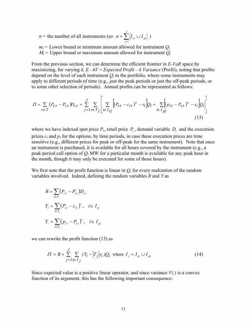
From the previous section, we can determine the efficient frontier in E-VaR space by maximizing, for varying k, E - kV = Expected Profit – k Variance (Profit), noting that profits depend on the level of each instrument Qi in the portfolio, where some instruments may apply to different periods of time (e.g., just the peak periods or just the off-peak periods, or to some other selection of periods). Annual profits can be represented as follows:

( ) ( )[ ] ( )[ ]∑ ∑ ∑ ∑ ∑∈ = ∈ ∈ ∈

++

−−+−−+−=

T

J

j jT cjIi pjIiiisiiiiscsc QsPpQrcPDPP

τ ττττττττΠ

1

(13) where we have indexed spot price Ps, retail price cP , demand variable cD and the execution prices ci and pi for the options, by time periods, in case these execution prices are time sensitive (e.g., different prices for peak or off-peak for the same instrument). Note that once an instrument is purchased, it is available for all hours covered by the instrument (e.g., a peak-period call option of Qi MW for a particular month is available for any peak hour in the month, though it may only be executed for some of those hours). We first note that the profit function is linear in Qi for every realization of the random variables involved. Indeed, defining the random variables R and Y as

( )∑∈

−=T

csc DPPRτ

τττ

( )∑∈

+ ∈−=jT

cjisi IicPYτ

ττ ,

( )∑∈

+ ∈−=jT

pjsii IiPpYτ

ττ ,

we can rewrite the profit function (13) as

∑ ∑= ∈

−+=J

j jIiiiji Q)rTY(R

1Π where pjcjj III ∪= (14)

Since expected value is a positive linear operator, and since variance V(.) is a convex function of its argument, this has the following important consequence:

12

Claim 3: For any fixed k > 0, the function Γ(Q, k) = E{Π (Q)} – kV{Π(Q)} is a concave function of Q = (Q1, ..., Qn). In fact, since profits in (14) are linear in Q, the structure of the optimal portfolio problem, Max E-kV, is simply a quadratic program that can be solved by existing algorithms, with structure as noted in the following proposition. Proposition 1: From (14), the function Γ(Q, k) whose maximization characterizes the efficient frontier in E-VaR space is given as follows: )}Q({kV)}Q({E)k,Q( ΠΠΓ −= (15) where

}R{EQE)}Q({En

iii += ∑

=1Π (16)

with

[ ]∑∈

∈−−=−=∂

∂=

jTcjijisiji

ii Ii,rT)c(G}P{ErT}Y{E

Q}{EE

ττττ

Π

[ ]∑=

∈−−=−=∂Π∂

=T

pjijiiijii

i IirTpGprTYEQ

EE1

,)(}{}{τ

τττ

∫ ∫∫∞

−+=+==v

vvs ))v(F(v)p(pdF)p(vdF)p(pdF]}v,P[Min{E)v(G

001 ττττττ

and where

RQAQQC}{V '' ++=vvvr

Π (17) with

)]',(2,),,(2[ 1 nYRCOVYRCOVC Lr=

})}Y{EY(})'Y{EY{(E)Y,Y(COVA −−== The claim above on the structure of Gτ is straightforward using the identiy (x-y)+ = Max(x-y, 0) = x – Min[x, y]. The remaining assertions in Proposition 1 are obvious from the structure of the profit function (14). From (15)-(17), the target function Γ(Q, k) = E – kV has the form:

13

)R(kV}R{EQAQkQH

)R(kV}R{EQAQkQ))Y,R(kCOV2E(

)R(kVQAQkQ))Y,R(COV2k}R{EQEkVE

'

'ii

n

1ii

'n

1iii

n

1iii

−+−=

−+−−=

−−−+=−

∑

∑∑

=

==

vvvv

vv

vv

(18)

where )k(H

v is the row vector with )Y,R(kCOVE)k(H iii 2−= .

Thus, maximizing kVE − is equivalent to maximizing QAQkQ)k(H ' vvvv

− . This is equivalent to maximizing a negative semi-definite quadratic form (since A is positive semi-definite, -A is negative semidefinite) subject to linear constraints on Q (namely upper and lower bounds on the Qi), which would has an easily determined solution via quadratic programming for each k and, using sensitivity analysis for varying k, just as it does in the usual portfolio optimization problem.17 Thus, one could use a standard quadratic programming code to solve this problem, just as in the normal portfolio optimization problem. For any given k, this yields E and V for the entire planning horizon of T periods. The VaR = VaR(k) corresponding to the optimal portfolio derived from maximizing (18) at the specified k is then derived directly or by simulation from the particulars of the underlying distributions (which need not be normal). Note that the quantities COV(R, Yi) and COV(Yi,Yj) can be computed once and for all as a part of the initialization phase, e.g., using Monte-Carlo simulation if the structure of the instruments of the characteristics of the underlying random variables describing spot price and demands/loads are complicated. These covariances do not depend on k, but only on the underlying givens of the problem (the spot price distributions and the reservation and execution cost parameters of the instruments in question). In particular, the spot price and demand distributions could well be correlated over time (they might arise, for example, from some regime switching stochastic process as described in Ethier and Mount (1998)). When underlying random variables are stochastically independent across specific sub-periods, e.g. from one month to the next, then a monthly optimization could be undertaken that would separate all instruments that have cashflows within the given month, and solve only the sub-problem associated with maximizing the separable part of (14) (or (15)) pertaining to the month in question. More generally, serial correlation for the underlying price and demand random variables is typically confined to successive weeks or months, so that the temporal structure of correlation is confined to a much shorter period of time than the entire year. Given this, the structure of the optimization problem implied by (14)-(15) is rather simple and can be addressed by a number of mathematical programming approaches. 17 To assure a solution, even in the unlikely event that K is not positive definite, one should impose upper and

lower bounds on each instrument decision variable Qi, where the bounds could be very large but finite. This is, of course, completely without any loss in generality, since there always would be upper and lower bounds on these instruments. The only time where there might be a problem is where k = 0, the pure expected profit-maximization problem.

14

The above framework solves the central problem of interest in this paper, namely the disaggregation of annual VaR constraints into sub-period VaR constraints. The solution is this. The annual problem is solved as above, by maximizing E – kV for varying k, yielding the efficient annual frontier. The Company then selects its desired annual VaR level, which implies an optimal k, together with associated optimal levels of sub-period instruments and sub-period VaRs. Equivalently, once the optimal annual E-V tradeoff value k is known, together with the associated monthly VaR level, this k can be used in a decentralized fashion on a monthly (sub-period) basis to optimize over available instruments. Indeed, any instrument Qi that makes an incremental, positive contribution to an existing portfolio, as measured by iQkVE ∂−∂ /)( , would be a positive addition to the existing portfolio. Similarly, one could analyze the optimal subset of contracts to add in a particular month to a given portfolio by maximizing (15), at the optimal annual k representing the risk appetite of the Company. One could also use the sub-period optimal VaR associated with the optimal annual k to monitor changes in VaR associated with incremental portfolio choices. The key is that the basic benchmark for ranking incremental portfolio choices is specified by E – kV, with k set at the optimal level. Together these facts yield operational rules, both for sub-period instrument ranking and choice as well as controls on VaR constraints. The analysis above does not require any assumptions on temporal separability of the instruments. For example, suppose that in addition to monthly instruments, there were choices of quarterly instruments and some annual choices related to the level of owned generation. Optimizing these latter instruments would require either solving the entire annual problem as a larger quadratic program or, more likely, using some search or decomposition procedure to optimize over the quarterly or annual instrument levels. For each setting of such levels, the monthly instruments could then easily be solved for based on the maximization of (15). Effectively, an annual instrument is an instrument that is constrained so that the level of execution of this instrument at each monthly sub-period is identical. Naturally, heuristic solutions and various search algorithms could also be used if there are more complicated constraints on the Qi variables, e.g., Boolean constraints of the sort that arise in capturing inter-dependencies in capital budgeting problems (Van Horne, 1966; Laughhunn, 1970) or maintenance or operational constraints that might apply to owned generation. The above framework thus leads to a general approach to solving both the single-period problem as well as the overall multi-period VaR problem. 4. Examples Let us consider a few examples to illustrate the above results. We structured a Company using PJM data (see Table 1 below). The Company faces a retail load that was taken to be 5% of the PJM load during the months of June-August, 2003. Spot price for the period was taken as the spot price at PJM West (a relatively liquid trading hub for electric power). The Company faces a regulated price of $50/MWh and has the option of structuring its portfolio of power assets using a number of sources to meet this retail load, as well as to engage in profitable trading with other firms in the power market. The information (probability distributions on price and demand) available to the Company for its planning was assumed to be the information available to traders and participants in PJM via the forward curve for

15

the respective months. For these examples, all statistical measures (e.g., correlations, variances) are obtained from Monte-Carlo simulations using WeatherDelta™ (a product of Sungard), which could provide simulated results in close to real time on means, variances and covariances of power prices, demands and trading instruments. The distributions for peak power and load profiles, as a result of the simulations, were well matched with historical distributions. We know from above that the efficient frontier is obtained by maximizing, for varying k, E – kV, which is equivalent to maximizing H(k)Q-kQ’AQ, with H(k), Q and A as defined above. As noted, the entries for H and A depend only on the means, variances and covariances of the returns on the individual instruments in the portfolio. This is a two-period problem with a combined VaR constraint over both periods. We also illustrate the problem of evaluating a multi-period investment option, in this case the possibility of adding an additional 50 MW generator available during the entire period of the portfolio.

Table 1: Basic Data for the Examples Mean Forecasted June On-Peak Price Ps Mean($/MWh) 50.5

Forecasted July/August On-Peak Price Mean($/MWh) 61.5

June Retail On-Peak Demand Dc (MW) 5% of PJM Load

July/August Retail On-Peak Demand Dc (MW) 5% of PJM Load

Retail Price Pc ($/MWh) 50

There are five types of potential assets in this portfolio: Generating units, monthly forward contracts, daily call options, daily put options and hourly call options. The time horizon for the portfolio is three months that will be considered as two-periods: June and July/August. The option contracts are assumed to be exercisable on a daily or hourly basis, but purchased for the entire month. Only peak hours are considered in this example. For simplicity, we assume transmission constraints, if any, are non-binding.18 Table 2 characterizes the available instruments for the portfolio. The reservation price ri for owned generation is 0 since we assume the Company is already committed to this. Similarly, the forward contract has an exercise price of 0 since, once signed, a forward is a contract requiring that the Company take delivery of the power purchased. Two types of generators are available. The first one has lower marginal costs but with an average $5/MWh fixed (reservation) cost. 18 The problem of transmission constraints deserves, of course, a much more extended treatment than a mere

passing remark. We neglect these details here, since our focus is on the portfolio problem and the multi-period VaR constraint. In markets such as PJM, where nodal pricing is used, the price of transmission links required for execution of contracts can and should be incorporated into the exercise price of the contracts in question (forwards or options). In other markets, where transmission must be separately contracted for, it is important current prices for reserving sufficient transmission capacity to exercise contracts be included as part of the contract pricing and feasibility structure. In such markets, some contracts come equipped with their own transmission capacity as part of the trade.

16

The second one is an owned generator, for which we therefore assume reservation cost ri = 0. However, it has higher marginal costs and is operational only in July and August. There are also two types of options in the portfolio, daily and hourly. The payoff for a daily option, once exercised, is calculated based on 16 peak hours, while the payoff for an hourly option is benchmarked on the respective hourly spot price. From the above results, the optimal portfolios are obtained by maximizing

AQkQQkH ')( − , with H(k) and A as defined above. For a fixed k, the resulting portfolio is on the leftmost border of the feasible set (which contains the efficient frontier) of E-VaR space. To define VaR, we use 95.0=γ for the confidence-level parameter. Using the WeatherDelta™ simulation for the period in question, we analyzed the distribution of cashflows for many portfolios. Picking off the 0.05 fractile of the resulting distribution of cashflows for each portfolio, we verified that RA was satisfied, and indeed the linear approximation φσσµγσµ == ).,,(h),,(h 950 provides an excellent fit for the period in question with the constantφ close to 1.9. (This implies that, as expected, the distribution is fatter tailed than the normal distribution, for which φ = 1.65 at γ = 0.95 would result.) Table 3 shows selected portfolios on the efficient frontier (indexed by their defining k) and a number of other (randomly generated, without index k) portfolios, which are clearly not on the efficient frontier. Figure 3 plots the efficient frontier and the random portfolios shown in Table 3. The left figure shows the efficient frontier in σ−E space (with both }{E Π and

}{Πσ being the values for all periods—June through August), while the right figure shows the efficient frontier in E-VaR space (again with }{E Π and }{ΠVaR being for all periods).

Table 2: Portfolio Components Asset Label ei ri mi Mi Jun Generation 1 25 5 500 500 Jun Forward 2 0 45 -400 400 Jun Daily Call 3 60 8 -300 300 Jun Daily Put 4 40 4.5 -300 300 Jun Daily Call 2 5 70 6 -300 300 Jun Daily Put 2 6 30 1.2 -300 300 Jun Hourly Call 7 60 9.5 -300 300 Jun Hourly Call 2 8 70 6.5 -300 300 Jul/Aug Gen. 1 9 25 5 500 500 Jul/Aug Gen. 2 10 30 0 400 400 Jul/Aug Forward 11 0 55 -400 400 Jul/Aug Daily Call 12 70 9 -300 300 Jul/Aug Daily Put 13 40 3 -300 300 Jul/Aug Daily Call 2 14 80 6 -300 300 Jul/Aug Daily Put 2 15 30 0.8 -300 300 Jul/Aug Hourly Call 16 70 10.5 -300 300 Jul/Aug Hourly Call 2 17 80 7.5 -300 300 The last set of figures is the result of adding a 50 MW slice of owned/leased generation to the feasible set of the previous portfolio, i.e. to Table 2. The execution price is assumed to be $25/MWh and the reservation price (fixed cost) is equivalent to $5/MWh. The reader may think of this as a very simple Power Purchase Agreement with a fixed (reservation) price of $5/MWh and an operating (or execution) cost of $25/MWh, which is clearly a very

17

desirable additional asset in the summer. Figure 4 superimposes the E-VaR efficient frontier of this portfolio on that of the corresponding E-VaR efficient frontier of Figure 3. While the additional generation increases the expected profit, it also contributes to adding standard deviation. On the other hand, since VaR characterizes only “down-side risk”, the new efficient frontier in E-VaR space is moved in a favorable direction (Figure 4) In this case, the movement is significant, since in the environment of summer’s high demands and high market prices the additional generation provides a more economic and stable supply for the base loads. If the additional generation reflected here were a planned acquisition, or a PPA with a fixed purchase price, then the cash flow coverage (required payment to capital providers) for the acquisition or purchase price would be subtracted from profits, allowing a joint evaluation of the effects of the additional generation on net profits and VaR, both evaluated at the resulting optimal portfolio. Of course, a much longer (e.g., 3-5 year) evaluation horizon (than our three-month example) would be appropriate in considering the benefits of generation acquisition.

Table 3 The Choice of k and Optimal Selection of Qi

k 2.0E-09 5.0E-09 1.0E-08 2.0E-08 5.0E-08 random random random random randomQ1 500 500 500 500 500 500 500 500 500 500Q2 400 400 400 400 400 400 400 300 300 400Q3 -300 -300 -300 -300 -300 200 200 300 300 -200Q4 300 300 300 300 300 -300 -300 -300 300 -200Q5 -300 -300 -300 -300 -300 200 -300 -300 100 100Q6 300 300 300 300 300 300 0 -200 -200 -200Q7 300 -207 -300 -300 -300 100 -300 300 -300 -300Q8 300 300 300 209 -10 250 250 0 100 100

H(k)-kQ'KQ 4641008 4541033 4476732 4358214 4156391 2018823 3603105 2767213 3316651 3753390E 2635345 2512582 2490067 2440762 2322102 2493689 2397784 2182578 2127415 2259868

E-kV 1764202 516011 -1461982 -5407885 -17091860 -6981799 -5397516 -6233408 -5683971 -5247231STD 20870349 19982847 19879760 19809905 19704802 22943756 20810387 21623015 20831847 20422073

June Assets

VaR 37018318 35454828 35281478 35198057 35117022 41099449 37141952 38901150 37453094 36542071Q9 500 500 500 500 500 500 500 500 500 500

Q10 400 400 400 400 400 400 400 300 300 400Q11 400 261 -87 -261 -400 100 100 100 0 200Q12 -300 -300 -300 -300 -300 200 100 100 100 100Q13 300 300 300 300 300 -200 0 0 200 -200Q14 -300 -300 -300 -300 -215 300 -300 -300 -300 300Q15 300 300 300 300 300 -100 300 300 300 300Q16 102 -300 -300 -300 -300 200 -300 -300 -300 -300Q17 300 300 300 300 300 300 300 300 300 -200

H(k)-kQ'KQ 19757147 18588548 17902311 17490458 17057332 -2330402 13239280 12485458 13568203 10713673E 4294693 3161510 1880683 1240269 778819 3838918 2675065 529434 166405 2342306

E-kV -1728652 -9995417 -22511930 -46584336 -117999119 -61673086 -46103403 -46857225 -45774480 -48629010STD 54878706 51297030 49388878 48900207 48739704 60328731 52056843 51308792 50520010 53214094

Jul/Aug Assets

VaR 99974849 94302847 91958185 91670124 91826618 110785670 96232937 96957271 95821614 98764473

E 6930038 5674091 4370749 3681031 3100921 6332607 5072849 2712012 2293819 4602175STD 58713234 55051789 53239704 52760426 52572217 64544339 56062350 55678963 54646475 56998253

Total

VaR 104625107 98924308 96784689 96563779 96786291 116301638 101445616 103078018 101534483 103694507

18

Figure 3: The Efficient Frontier for Portfolios Resulting from Table 3 Instruments

Figure 4: Efficient Frontier

Figure 4: Efficient Frontier With (Squares) and Without (Diamonds) Additional Generator

5. Conclusions This paper has considered the multi-period, VaR-constrained portfolio optimization problem and its application to electric power. The problem is motivated by the fact that electric power trading and procurement (and many other applications) typically entails portfolio choice problems having different temporal commitment dates, with some instruments covering weekly contracts, some monthly and some for longer periods. Absent a unifying framework, implementing VaR constraints for these problems has been somewhat

0

1000000

2000000

3000000

4000000

5000000

6000000

7000000

8000000

Sigm a{Pi}

E{Pi

}

0

1000000

2000000

3000000

4000000

5000000

6000000

7000000

8000000

9000000

Sigm a{Pi}

E{Pi

}

0

1000000

2000000

3000000

4000000

5000000

6000000

7000000

8000000

9000000

VaR

E{Pi

}

0

1000000

2000000

3000000

4000000

5000000

6000000

7000000

8000000

VaR

E{Pi

}

19

haphazard and has involved various approximations that typically do not implement the VaR constraint in a satisfactory fashion for sub-periods of the overall planning horizon. The present paper is a first step in developing such a unified framework. We have shown that, just as in the σ−E efficient frontier determination for standard portfolio analysis, the problem of interest here can be represented in a fashion that is both computationally efficient, using readily available simulation and optimization methods, as well as yielding appropriate managerial yardsticks for the implementation of VaR-constrained trading. We have pointed out a number of limitations along the way that serve as pointers for future research. We have imposed a regularity condition on the distribution of cashflows that appears to be consistent with simulations for an annual or seasonal planning horizon. We have tested this (RA) approach in Kleindorfer and Li (2004) and it appears to hold up well for real power sector data. But further testing and refinement of this approach would be desirable. For longer planning horizons, it would also be interesting to consider technological and price uncertainty for generation acquisiton, as well as POLR (Provider of Last Resort) and other regulatory obligations that could impact the profit distribution of portfolios. Finally, we have considered neither transmission constraints nor credit constraints (the latter on trading settlement procedures). Credit risks could be included in the above framework by having the cashflows associated with the execution of puts and calls themselves be random variables (e.g., if Qi MW are contracted and called, then expected cashflows are (1-ρi)Qi times the strike price, where ρi is the default risk), but transmission constraints are likely to be difficult to deal with given current uncertainties about the changes in transmission markets. There are also many other practical issues that need to be considered in integrating the proposed approach with currently existing power market simulation tools and trading platforms. The questions involved include how frequently to update the optimal k, driving sub-period optimizations and VaRs; and the length of sub-periods to be included in controlling VaR at a sub-period level. These issues suggest a rich pallet of interesting future research in understanding how to remove some of the limitations imposed here and how to implement this framework in practice. Appendix Proof of Claim 1: First we look at VE − space. (See Figure 1) The equation ckVE += defines a straight line for any constant c. Thus, maximizing )}Q({kV)}Q({E ΠΠ − is equivalent to maximizing c, or maximizing E-kV, such that line ckVE += just meets the feasible portfolio set. Thus, any Q maximizing )}Q({kV)}Q({E ΠΠ − must be on the efficient frontier in E-V space. This same Q must clearly also be on the efficient frontier in σ−E space (since any portfolio Q’ with the same or equal expected payoff and smaller variance, must also have smaller standard deviation). Now we show that this same portfolio is on the left border in E-VaR space. Suppose Q has expected profit E1 and standard deviation 1σ . If there is a portfolio with expected profit and VaR, say E2 and VaR2, such that E1 = E2 and 12 VaRVaR < , then by (5)

111222 ),,(),,( EEhEEh −<− γσγσ and therefore we have ),,E(h),,E(h γσγσ 1122 < , so that the monotonicity of h in σ implies 12 σσ < . This is impossible since Q was assumed to be on the

σ−E frontier. Thus, Q must be on the left border of the feasible set in E-VaR space.

20

Proof of Claim 2: We first show that any portfolio, say Q1, on the efficient frontier in E-VaR space, say yielding (E1,VaR1), is also on the frontier in σ−E space (and therefore is also an image of a frontier portfolio in VE − space). In fact, if there is a portfolio Q2 yielding ),( 22 σE with 12 EE ≥ and 12 σσ ≤ then (E2, VaR2) = )),,(,( 2222 EEhE −γσ in E-VaR space satisfies 12 EE ≥ and, from RA,

VaR2 = 1111121222 ),,(),,(),,( VaREEhEEhEEh =−≤−≤− γσγσγσ as VaR is non-increasing in E and h is increasing in σ. But then 12 EE = and 12 σσ = since

),( 11 VaRE was assumed to be on the frontier of E-VaR space, yielding the desired result that ),( 11 σE is also on the frontier in σ−E space. So as long as we can show that any frontier

portfolio in E-V space (or equivalently in σ−E space) is the solution to E-kV for some k, the claim is established. We now show that the frontier in E-V space is (strictly) concave so that, indeed, every frontier portfolio is the solution to E-kV for some k. It is well known, e.g. Sharpe (2000), that with linear constraints, the efficient frontier in σ−E space is concave. Equivalently, if ),(),,( 2211 σσ EE and ),( 33 σE are on the frontier and

213 )1( EEE αα −+= for some α , with 0 < α < 1, then .)1( 213 σαασσ −+≤ Now we will show that the efficient frontier in E-V space is also concave. That is, for the same portfolios, we wish to show .)1( 2

221

23 σαασσ −+≤ In fact,

2122

221

223 )1(2)1( σσαασασασ −+−+≤

so that

0))((

])1([)1(2)1(])1([2

212

22

2121

22

221

222

21

23

<−−=

−+−−+−+≤−+−

σσαα

σαασσσαασασασαασσ

Therefore .)1( 2

221

23 σαασσ −+< From the (strict19) concavity of the efficient frontier in E-V

space, we see that if Q is on the frontier in E-V space, there will be a straight line tangent to the frontier curve at Q. Choosing k as the slope of this line, and maximizing E - kV will result in the (E, V) of the portfolio Q, completing the proof of the claim. References Artzner, P., F. Delbaen, J-M. Eber and D. Heath. 1999. “Coherent Risk Measures”, Mathematical Finance, Vol. 9, 203-228.

19 Thus, while a portion of the efficient frontier can be linear in σ−E space as depicted in Figure 2 (e.g.,

when the profits of a set of efficient portfolios are perfectly correlated), this cannot happen in E-V space.

21

Artzner, P., F. Delbaen, J-M. Eber, D. Heath and H. Ku. 2002. “Coherent Multiperiod Risk Management”, Working Paper, RiskLab, ETH, Zurich. Banerjee, S. and T. Noe. 2002. “Exotics and Electrons: Electric Power Crises and Financial Risk Management,” Presented at Berlin Meeting of European Finance Association. Bertsekas, D. P., 1995. Dynamic Programming and Optimal Control, Athena Scientific, Belmont, MA. Bessembinder, H. and M. Lemmon, 2002. “Equilibrium pricing and optimal hedging in electricity forward markets,” Journal of Finance, 57: 1347-1382. Brealey R. A. and S. C. Myers, 1991. Principles of Corporate Finance. 4th edition, McGraw Hill. Brigo,D., F. Mercurio, 2002. “Lognormal-Mixture Dynamics and Calibration to Market Volatility Smiles,” International Journal of Theoretical and Applied Finance. Vol. 5, No. 4, 427-446. California Assembly Bill, AB 57, Chapter 835, September 24, 2002. Clewlow, L. and C. Strickland, 2000. Energy Derivatives: Pricing and Risk Management. Lacima Publications, London. Coronado, M., 2000. “Comparing Different Methods for Estimating Value-at-Risk (VaR) for Actual Non-Linear Portfolios: Empirical Evidence”, Working paper, Facultad de Ciencias Economicas y Empresariales, ICADE, Universidad P. Comillas de Madrid, Madrid, Spain. Crouhy, M., D. Galai and R. Mark, 2000, Risk Management, McGraw Hill, New York. EIA, 2002. Derivatives and Risk Management in the Petroleum, Natural Gas and Electricity Industries, Energy Information Administration, US Department of Energy, Washington D.C. Ethier, R. and T. Mount, 1998. “Estimating the Volatility of Spot Prices in Restructured Electricity Markets and the Implications for Option Values,” Working Paper. Cornell University. Eydeland A. and K. Wolyniec, 2003. Energy and Power Risk Management: New Development in Modeling, Pricing and Hedging, New York, NY: John Wiley. Haigh, M.S. and M.T. Holt, 2002. “Combining time-varying and dynamic multi-period optimal hedging models,” European Review of Agricultural Economics, 29(4): 471-500. Hull, J. C. and A. White, 1998. “Value and Risk when Daily Changes in Market Variables are not Normally Distributed,” J. of Derivatives, Vol. 5, No. 3 (Spring), 9-19.

22

Humphreys, H.B. and K.T. McClain, 1998. “Reducing the impact of energy price volatility through dynamic portfolio selection,” Energy Journal 19(3): 107-131. Kamat, R. and S. Oren,. 2002. “Exotic Options for Interruptible Electricity Supply Contracts.” Operations Research, 835-850.

Kleindorfer, P. R. and D.J. Wu, 2003. “Integrating Long-term and Short-term Contracting via Business-to-Business Exchanges for Capital-Intensive Industries,” Management Science, Vol. 49, No. 11, 1597-1615. Laughhunn, D.J., 1970. “Quadratic Binary Programming with Applications to Capital Budgeting Problems”. Operations Research, Vol. 18, 454-461. Markowitz, H. M., 1952. “Portfolio Selection”, Journal of Finance, Vol. 7, March, 77-91. Marshall, C. and M. Siegel, 1997. “Value at Risk: Implementing a Risk Measurement Standard,” J. of Derivatives, Vol. 4 (Spring), 91-110. Morari, M. and J. H. Lee, 1999. "Model Predictive Control: Past, Present and Future," Computers and Chemical Engineering. Vol 23, 667-682. Mount, T., 2002. “Using weather derivatives to improve the efficiency of forward markets for electricity.” In: R.H. Sprague, Jr. (Ed.), Proceedings of the Thirty-Fifth Annual Hawaii International Conference on System Sciences, IEEE Computer Society Press, Los Alamitos, California, 2002. Rockafeller, R. T. and S. Uryasev, 2000. “Optimization of Conditional Value-at-Risk,” J. of Risk, Vol. 2, No. 3, 21-41. Sharpe, W., 2000. Portfolio Theory & Capital Markets, McGraw-Hill, New York. Sweeney, J. L. 2002. The California Electricity Crisis, Hoover Institution Press, Stanford, CA. Van Horne, J., 1966. “Capital-Budgeting Decisions Involving Combinations of Risky Investments”, Management Science, October, 84-92. Woo, C.K., R. Karimov, and I. Horowitz 2004. “Managing electricity procurement cost and risk by a local distribution company,” Energy Policy, 32(5): 635-645.

Kleindorfer, P.R. and L. Li, 2004. “Note on Value-at-Risk Measurement for Non-Gaussian Distributions” 2004. Working Paper, Wharton Center for Risk Management and Decision Processes, University of Pennsylvania.

23

Woo, C.K., I. Horowitz, B. Horii, and R. Karimov 2003. “The efficient frontier for spot and forward purchases: an application to electricity,” Journal of the Operational Research Society, forthcoming.