Multi-period reverse logistics network design

European Journal of Operational Research 220 (2012) 67–78

Contents lists available at SciVerse ScienceDirect

European Journal of Operational Research

journal homepage: www.elsevier .com/locate /e jor

Production, Manufacturing and Logistics

Multi-period reverse logistics network design

Sibel A. Alumur a,⇑, Stefan Nickel b,c, Francisco Saldanha-da-Gama d, Vedat Verter e

a Department of Industrial Engineering, TOBB University of Economics and Technology, Ankara, Turkeyb Institute for Operations Research, Karlsruhe Institute of Technology (KIT), Karlsruhe, Germanyc Fraunhofer Institute for Industrial Mathematics (ITWM), Kaiserslautern, Germanyd DEIO-CIO, Faculdade de Ciências, Universidade de Lisboa, Lisboa, Portugale Desautels Faculty of Management, McGill University, Montreal, Canada

a r t i c l e i n f o

Article history:Received 9 January 2011Accepted 19 December 2011Available online 15 January 2012

Keywords:LogisticsLocationWEEELarge household appliances

0377-2217/$ - see front matter � 2012 Elsevier B.V. Adoi:10.1016/j.ejor.2011.12.045

⇑ Corresponding author. Tel.: +90 532 3619960; faxE-mail addresses: [email protected] (S.A. Alum

(S. Nickel), [email protected] (F. Saldanha-da-Gama(V. Verter).

a b s t r a c t

The configuration of the reverse logistics network is a complex problem comprising the determination ofthe optimal sites and capacities of collection centers, inspection centers, remanufacturing facilities, and/or recycling plants. In this paper, we propose a profit maximization modeling framework for reverselogistics network design problems. We present a mixed-integer linear programming formulation thatis flexible to incorporate most of the reverse network structures plausible in practice. In order to considerthe possibility of making future adjustments in the network configuration to allow gradual changes in thenetwork structure and in the capacities of the facilities, we consider a multi-period setting. We propose amulti-commodity formulation and use a reverse bill of materials in order to capture component com-monality among different products and to have the flexibility to incorporate all plausible means in tack-ling product returns. The proposed general framework is justified by a case study in the context of reverselogistics network design for washing machines and tumble dryers in Germany. We conduct extensiveparametric and scenario analysis to illustrate the potential benefits of using a dynamic model as opposedto its static counterpart, and also to derive a number of managerial insights.

� 2012 Elsevier B.V. All rights reserved.

1. Introduction

Extended producer responsibility is becoming increasingly com-mon around the globe. In the electronics sector, for example, 26states in the U.S., most Canadian provinces, the European Unionand Japan have enacted regulations that require the original equip-ment manufacturers (OEMs) to ensure environmentally safe dis-posal of their end-of-life products. In order to comply with theenvironmental legislation, firms in many industries find themselvesfacing the challenge of developing their reverse logistics capabili-ties. Reverse logistics is the process of planning, implementingand controlling backward flows of raw materials, in process inven-tory, packaging and finished goods, from a manufacturing, distribu-tion or use point, to a point of recovery or point of proper disposal(REVLOG, 1998). In the broadest sense, this process involves collec-tion, inspection, recycling, refurbishing, and remanufacturing ofused or returned products, including leased equipment andmachines.

An OEM’s direct involvement with the reverse logistics processis usually a function of the economic value that can be captured by

ll rights reserved.

: +90 312 2924091.ur), [email protected]

), [email protected]

processing the returned products. When this constitutes a net costfor the OEM, the collected items are typically send to recycling thatis performed by a third party. In satisfying the recycling targetsstipulated by the European Union WEEE Directive (2002), forexample, many OEMs have outsourced the administration of thereverse logistics process to collective take-back schemes, whopay the recyclers utilizing the fees charged to the OEMs. Whenthe OEM can generate economic value from product recovery,however, establishing its own reverse logistics network – that of-ten includes remanufacturing facilities – becomes viable. Well-known examples of this group include HP, Xerox, Caterpillar, andKodak. There are also product groups where the economic benefitsof remanufacturing are not viable to OEM, but third party reman-ufacturers can generate sizeable profits. Cell phones are a goodexample of this third group, since major manufacturers includingNokia and Ericsson are not involved in remanufacturing.

In this paper, we focus on return streams with profit potentialfor the OEM. For instance, computers contain precious metals suchas gold and silver, which remain intact until a computer becomesobsolete. Indeed, one ton of such electronic waste contains moregold that 17 tons of material extracted from a gold mine (Bleiwasand Kelly, 2001). In addition, a number of components can be ex-tracted from an end-of-use computer that can be used for reman-ufacturing and sold in secondary markets. Washing machines andtumble dryers constitute another example. In addition to their

68 S.A. Alumur et al. / European Journal of Operational Research 220 (2012) 67–78

steel content, which can be recovered through recycling; there is ahealthy secondary market for remanufactured washing machinesand tumble dryers, i.e., coin laundries and coin-op machines inapartment buildings. For such product groups, the configurationof the reverse logistics network is a complex problem. It comprisesdetermining the optimal sites and capacities of collection centers,inspection centers, remanufacturing facilities, and/or recyclingplants. There is an increasing interest in this problem and a recentreview of the literature can be found in Aras et al. (2010).

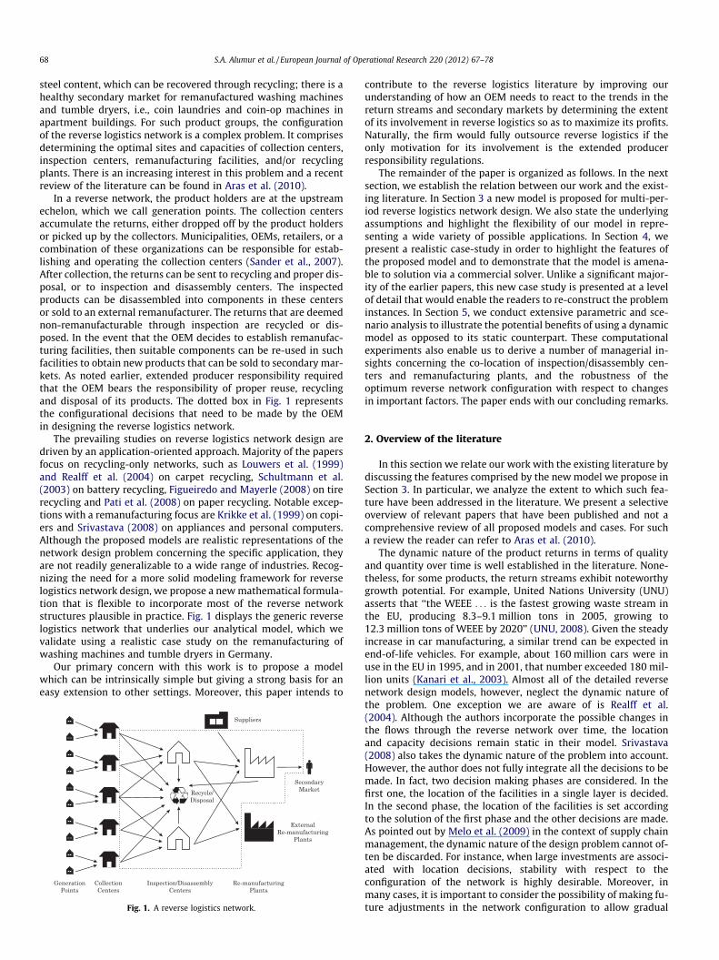
In a reverse network, the product holders are at the upstreamechelon, which we call generation points. The collection centersaccumulate the returns, either dropped off by the product holdersor picked up by the collectors. Municipalities, OEMs, retailers, or acombination of these organizations can be responsible for estab-lishing and operating the collection centers (Sander et al., 2007).After collection, the returns can be sent to recycling and proper dis-posal, or to inspection and disassembly centers. The inspectedproducts can be disassembled into components in these centersor sold to an external remanufacturer. The returns that are deemednon-remanufacturable through inspection are recycled or dis-posed. In the event that the OEM decides to establish remanufac-turing facilities, then suitable components can be re-used in suchfacilities to obtain new products that can be sold to secondary mar-kets. As noted earlier, extended producer responsibility requiredthat the OEM bears the responsibility of proper reuse, recyclingand disposal of its products. The dotted box in Fig. 1 representsthe configurational decisions that need to be made by the OEMin designing the reverse logistics network.

The prevailing studies on reverse logistics network design aredriven by an application-oriented approach. Majority of the papersfocus on recycling-only networks, such as Louwers et al. (1999)and Realff et al. (2004) on carpet recycling, Schultmann et al.(2003) on battery recycling, Figueiredo and Mayerle (2008) on tirerecycling and Pati et al. (2008) on paper recycling. Notable excep-tions with a remanufacturing focus are Krikke et al. (1999) on copi-ers and Srivastava (2008) on appliances and personal computers.Although the proposed models are realistic representations of thenetwork design problem concerning the specific application, theyare not readily generalizable to a wide range of industries. Recog-nizing the need for a more solid modeling framework for reverselogistics network design, we propose a new mathematical formula-tion that is flexible to incorporate most of the reverse networkstructures plausible in practice. Fig. 1 displays the generic reverselogistics network that underlies our analytical model, which wevalidate using a realistic case study on the remanufacturing ofwashing machines and tumble dryers in Germany.

Our primary concern with this work is to propose a modelwhich can be intrinsically simple but giving a strong basis for aneasy extension to other settings. Moreover, this paper intends to

Fig. 1. A reverse logistics network.

contribute to the reverse logistics literature by improving ourunderstanding of how an OEM needs to react to the trends in thereturn streams and secondary markets by determining the extentof its involvement in reverse logistics so as to maximize its profits.Naturally, the firm would fully outsource reverse logistics if theonly motivation for its involvement is the extended producerresponsibility regulations.

The remainder of the paper is organized as follows. In the nextsection, we establish the relation between our work and the exist-ing literature. In Section 3 a new model is proposed for multi-per-iod reverse logistics network design. We also state the underlyingassumptions and highlight the flexibility of our model in repre-senting a wide variety of possible applications. In Section 4, wepresent a realistic case-study in order to highlight the features ofthe proposed model and to demonstrate that the model is amena-ble to solution via a commercial solver. Unlike a significant major-ity of the earlier papers, this new case study is presented at a levelof detail that would enable the readers to re-construct the probleminstances. In Section 5, we conduct extensive parametric and sce-nario analysis to illustrate the potential benefits of using a dynamicmodel as opposed to its static counterpart. These computationalexperiments also enable us to derive a number of managerial in-sights concerning the co-location of inspection/disassembly cen-ters and remanufacturing plants, and the robustness of theoptimum reverse network configuration with respect to changesin important factors. The paper ends with our concluding remarks.

2. Overview of the literature

In this section we relate our work with the existing literature bydiscussing the features comprised by the new model we propose inSection 3. In particular, we analyze the extent to which such fea-ture have been addressed in the literature. We present a selectiveoverview of relevant papers that have been published and not acomprehensive review of all proposed models and cases. For sucha review the reader can refer to Aras et al. (2010).

The dynamic nature of the product returns in terms of qualityand quantity over time is well established in the literature. None-theless, for some products, the return streams exhibit noteworthygrowth potential. For example, United Nations University (UNU)asserts that ‘‘the WEEE . . . is the fastest growing waste stream inthe EU, producing 8.3–9.1 million tons in 2005, growing to12.3 million tons of WEEE by 2020’’ (UNU, 2008). Given the steadyincrease in car manufacturing, a similar trend can be expected inend-of-life vehicles. For example, about 160 million cars were inuse in the EU in 1995, and in 2001, that number exceeded 180 mil-lion units (Kanari et al., 2003). Almost all of the detailed reversenetwork design models, however, neglect the dynamic nature ofthe problem. One exception we are aware of is Realff et al.(2004). Although the authors incorporate the possible changes inthe flows through the reverse network over time, the locationand capacity decisions remain static in their model. Srivastava(2008) also takes the dynamic nature of the problem into account.However, the author does not fully integrate all the decisions to bemade. In fact, two decision making phases are considered. In thefirst one, the location of the facilities in a single layer is decided.In the second phase, the location of the facilities is set accordingto the solution of the first phase and the other decisions are made.As pointed out by Melo et al. (2009) in the context of supply chainmanagement, the dynamic nature of the design problem cannot of-ten be discarded. For instance, when large investments are associ-ated with location decisions, stability with respect to theconfiguration of the network is highly desirable. Moreover, inmany cases, it is important to consider the possibility of making fu-ture adjustments in the network configuration to allow gradual

S.A. Alumur et al. / European Journal of Operational Research 220 (2012) 67–78 69

changes in the network structure and/or in the capacities of thefacilities. To fill this gap in the reverse network design literature,we present a multi-period model of the reverse network designproblem.

The OEMs are constantly introducing new products in an effortto sustain/increase their market share. This contributes to the dy-namic nature of the return streams, since the new products startappearing among the returned items after a certain time lag, e.g.,the average lifespan of a car in use is 12–15 years. Note that themajor switch in the display device production technology fromCRT monitors to flat LCD panels is expected to impact the streamof returned units in the coming years. In this paper, we use a mul-ti-commodity formulation so as to be able to incorporate these ma-jor trends in the reverse network design. We also use a reverse billof materials in order to capture component commonality amongdifferent products and to have the flexibility to incorporate mostof the plausible means an OEM can adopt in tackling product re-turns. By using reverse BOM, the model also addresses the possibil-ity of sending certain components to recycling/disposal and thepossibility of purchasing new components for remanufacturing.To the best of our knowledge, Jayaraman et al. (1999) is the firstpaper that studied a multi-product model of reverse logistics. Morerecently, Listes� and Dekker (2005), Pati et al. (2008), Srivastava(2008), Fonseca et al. (2010), and Gomes et al. (2011) also pre-sented multi-product formulations.

In order to focus on the dynamic nature of the problem, whilekeeping the mathematical model generic and tractable, we ignoreuncertainties that can be important in some contexts. The readeris referred to Realff et al. (2004), Fonseca et al. (2010), Listes� andDekker (2005), and Lieckens and Vandaele (2007) for reverse net-work design models that incorporate stochastic factors. Our mod-eling framework is applicable when the OEM has fairly reliableestimates of the amount of returns to be collected during the plan-ning horizon as well as the demand at the secondary market forremanufactured products.

Typically, an OEM is provided with modular capacity options forexpanding its inspection/disassembly and remanufacturing capa-bilities. Different modules options can be driven for instance fromdifferent available technologies. In this case, by choosing thecapacity of a facility the type of technology employed is also beingchosen. The reader can refer to Fonseca et al. (2010) for further de-tails. To the best of our knowledge, the adjustment of capacitydecisions over time in a reverse logistics network design problemhas been attempted only by Srivastava (2008). Discrete capacityexpansions are allowed for the facilities. In the sequential model-ing framework adapted by the author, such decisions are madein the second decision making phase, and thus are not taken intoaccount when the location decisions are made. Our model deter-mines if and where to establish the OEM’s facilities and the pro-gression of their capacity over time. The amount of returns to bedisposed, recycled, and remanufactured by third parties are deter-mined simultaneously.

Although the integration of the OEM’s forward and reverse net-works is out of the scope of this paper we would like to point outthat much work has been done in this area. In particular, severalpapers can be found in the literature addressing case studies in thiscontext. This is the case with Fleischmann et al. (2001) on papercopiers, Krikke et al. (2003) on refrigerators and Salema et al.(2009) on office document company. The dynamic nature of thesenetwork design problems is captured by Lee and Dong (2009) andSalema et al. (2010). For a deeper review of the growing literatureon closed-loop supply chains we refer the reader to Aras et al.(2010).

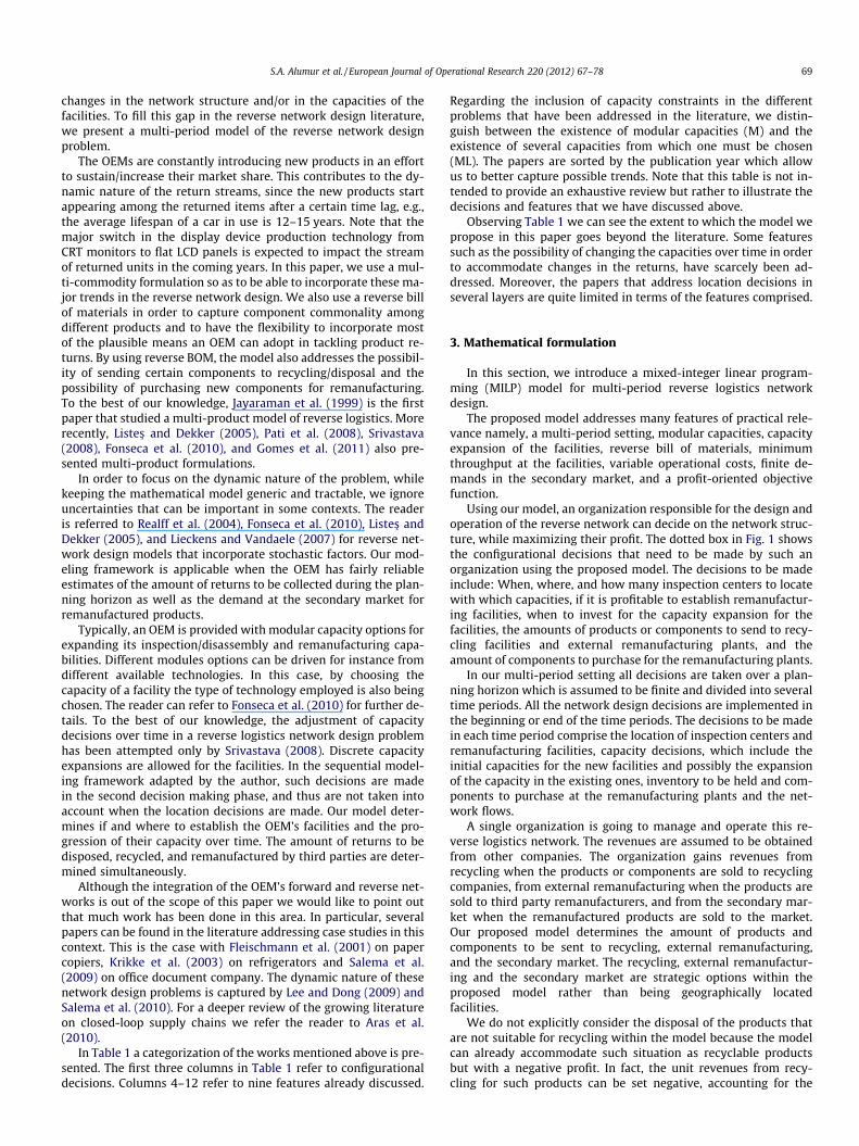
In Table 1 a categorization of the works mentioned above is pre-sented. The first three columns in Table 1 refer to configurationaldecisions. Columns 4–12 refer to nine features already discussed.

Regarding the inclusion of capacity constraints in the differentproblems that have been addressed in the literature, we distin-guish between the existence of modular capacities (M) and theexistence of several capacities from which one must be chosen(ML). The papers are sorted by the publication year which allowus to better capture possible trends. Note that this table is not in-tended to provide an exhaustive review but rather to illustrate thedecisions and features that we have discussed above.

Observing Table 1 we can see the extent to which the model wepropose in this paper goes beyond the literature. Some featuressuch as the possibility of changing the capacities over time in orderto accommodate changes in the returns, have scarcely been ad-dressed. Moreover, the papers that address location decisions inseveral layers are quite limited in terms of the features comprised.

3. Mathematical formulation

In this section, we introduce a mixed-integer linear program-ming (MILP) model for multi-period reverse logistics networkdesign.

The proposed model addresses many features of practical rele-vance namely, a multi-period setting, modular capacities, capacityexpansion of the facilities, reverse bill of materials, minimumthroughput at the facilities, variable operational costs, finite de-mands in the secondary market, and a profit-oriented objectivefunction.

Using our model, an organization responsible for the design andoperation of the reverse network can decide on the network struc-ture, while maximizing their profit. The dotted box in Fig. 1 showsthe configurational decisions that need to be made by such anorganization using the proposed model. The decisions to be madeinclude: When, where, and how many inspection centers to locatewith which capacities, if it is profitable to establish remanufactur-ing facilities, when to invest for the capacity expansion for thefacilities, the amounts of products or components to send to recy-cling facilities and external remanufacturing plants, and theamount of components to purchase for the remanufacturing plants.

In our multi-period setting all decisions are taken over a plan-ning horizon which is assumed to be finite and divided into severaltime periods. All the network design decisions are implemented inthe beginning or end of the time periods. The decisions to be madein each time period comprise the location of inspection centers andremanufacturing facilities, capacity decisions, which include theinitial capacities for the new facilities and possibly the expansionof the capacity in the existing ones, inventory to be held and com-ponents to purchase at the remanufacturing plants and the net-work flows.

A single organization is going to manage and operate this re-verse logistics network. The revenues are assumed to be obtainedfrom other companies. The organization gains revenues fromrecycling when the products or components are sold to recyclingcompanies, from external remanufacturing when the products aresold to third party remanufacturers, and from the secondary mar-ket when the remanufactured products are sold to the market.Our proposed model determines the amount of products andcomponents to be sent to recycling, external remanufacturing,and the secondary market. The recycling, external remanufactur-ing and the secondary market are strategic options within theproposed model rather than being geographically locatedfacilities.

We do not explicitly consider the disposal of the products thatare not suitable for recycling within the model because the modelcan already accommodate such situation as recyclable productsbut with a negative profit. In fact, the unit revenues from recy-cling for such products can be set negative, accounting for the

Table 1Reverse logistics features in addition to the location of the reverse facilities.

Article Location decisions for reverse activities Multipleproducts

ReverseBOM

Dynamicreturns

Dynamiclocation

Capacities Timeadjustmentcapacities

Minimumthroughput

Profitoriented

Secondarymarket

Inspectiondisassembly

Recycling Remanufacturingrefurbishing

Jayaraman et al.(1999)

p pC

Krikke et al.(1999)

p

Louwers et al.(1999)

p p p

Fleischmannet al. (2001)

p p

Schultmann et al.(2003)

p pC

Krikke et al.(2003)

p p p p p

Realff et al.(2004)

p p p p p pC

p p

Listes� and Dekker(2005)

p p pC

p p

Lieckens andVandaele

(2007)

p pML

p p

Figueiredo andMayerle(2008)

p

Pati et al. (2008)p p p

CSalema et al.

(2009)

p p p pC

p p

Srivastava (2008)p p

Cp p

Fonseca et al.(2010)

p p p pM

Gomes et al.(2011)

p p p p pC

The new modelp p p p p p p

Mp p p p

‘C’: Capacitated‘M’: Modular capacities‘ML’: Multi-level capacities

70 S.A. Alumur et al. / European Journal of Operational Research 220 (2012) 67–78

cost of disposal, for example, defined by the fee to be paid to sendthe product to an appropriate disposal facility such as a landfill.In such a case, the products that need to be disposed can beforced to be sent to recycling.

In our model, all the components are assumed to be suitablefor remanufacturing. However, in practice this is not the case be-cause some of them can be damaged and thus not re-usable.There is no need to distinguish this situation in the model asthe components that are not suitable for remanufacturing canbe sent to disposal and the corresponding costs (of both disposaland of buying new components to replace the damaged ones) canbe included in the operational costs.

We start by presenting the notation. Afterwards, we introducethe proposed MILP formulation.

3.1. Notation

In order to propose a MILP model for the problem the followingnotation is introduced.SetsP set of products (disposals)C set of componentsCp set of components for product p 2 P (Cp � C)T set of periods in the planning horizonIG set of generation points or collection centersII set of potential locations for inspection centersIR set of potential locations for remanufacturing plantsRG recycling node for collection centersRI recycling node for inspection centersRR recycling node for remanufacturing plantsER external remanufacturing plants

SM secondary marketQI set of capacities of the modules available for inspection

centersQR set of capacities of the modules available for remanufac-

turing plants

Available channels for the flow:

A ¼ fði; jÞ : ði 2 IG ^ j 2 IIÞ or ði 2 IG ^ j 2 RGÞ [ fði; jÞ : ði 2 II ^ j

2 IRÞ or ði 2 II ^ j 2 RIÞ or ði 2 II ^ j 2 ERÞg [ fði; jÞ : ði 2 IR ^ j

2 RRÞg or ði 2 IR ^ j 2 SMÞ

General parametersSt

ip supply of product or disposal p 2 P from collection centeri 2 IG in period t 2 T

Dtp demand of the secondary market for product p 2 P in per-

iod t 2 Tapc amount of component c 2 Cp in one unit of product p 2 PcIp unit capacity consumption factor for product p 2 P for

inspectioncRp unit capacity consumption factor for product p 2 P for

remanufacturingcc unit inventory capacity consumption factor for component

c 2 CMIt

i minimum throughput required for an inspection center lo-cated at i 2 II in period t 2 T

MRti minimum throughput required for a remanufacturing

plant located at i 2 IR in period t 2 TKERt

i capacity of the external remanufacturing plant located ati 2 ER in period t 2 T

MaxXt2T

Xp2P

Xi2IG

PRGtpxt

iRGpþXc2C

Xi2II

PRItcxt

iRI cþXc2C

Xi2IR

PRRtcxt

iRRc

24

þXp2P

Xi2II

Xj2ER

PERtjpxt

ijp þXp2P

Xi2IR

PSMtpxt

iSMp

#

�Xt2T

Xi2II

FIti yt

i � yt�1i

� �þXi2IR

FRti zt

i � zt�1i

� �" #

�Xt2T

Xi2II

Xq2QI

FKItiqut

iq þXi2IR

Xq2QR

FKRtiqv t

iq

24

35

�Xt2T

Xp2P

Xi2IG

Xj2II

OItjpxt

ijp þXi2IR

ORtipxt

iSMp

24

35

�Xt2T

Xp2P

Xi2IG

Xj2II

Ttijpxt

ijp þXc2C

Xi2II

Xj2IR

Ttijcxt

ijc

24

35

�Xt2T

Xc2C

Xi2IR

ICticIt

ic

�Xt2T

Xc2C

Xi2IR

BCticbt

ic; ð1Þ

s:t: Stip ¼ xt

iRGpþXj2II

xtijp; i 2 IG; p 2 P; t 2 T; ð2Þ

Xj2IG

xtjip ¼

Xj2ER

xtijp þ

1apc

xtiRIcþXj2IR

1apc

xtijc;

i 2 II;p 2 P; c 2 Cp; t 2 T; ð3ÞXj2II

xtjic þ It�1

ic þ btic ¼ xt

iRRcþ apcxt

iSMp þ Itic;

i 2 IR; p 2 P; c 2 Cp; t 2 T; ð4ÞXi2IR

xtiSMp 6 Dt

p; p 2 P; t 2 T; ð5Þ

Xi2II

Xp2P

xtijp 6 KERt

j ; j 2 ER; t 2 T; ð6Þ

Xj2IG

Xp2P

cIpxtjip 6

Xt

s¼1

Xq2QI

KIqusiq; i 2 II; t 2 T; ð7Þ

Xt

Xt Xs R

S.A. Alumur et al. / European Journal of Operational Research 220 (2012) 67–78 71

KIq capacity of inspection of a module of type q 2 QI

KPq production capacity of a module of type q 2 QR

KHq inbound handling capacity of a module of type q 2 QR

KINq inventory holding capacity of a module of type q 2 QR

RevenuesPRGt

p unit revenue from product p 2 P recycled from a collectioncenter in period t 2 T

PRItc unit revenue from component c 2 C recycled from an

inspection center in period t 2 TPRRt

c unit revenue from component c 2 C recycled from aremanufacturing plant in period t 2 T

PERtip unit revenue from product p 2 P sold to an external reman-

ufacturing plant at i 2 ER in period t 2 TPSMt

p unit revenue from product p 2 P sold to the secondarymarket in period t 2 T

It is assumed that the values above represent discounted values,i.e., the inflation rate has been discounted and thus that all themonetary values report to the current value on money.

CostsFIt

i set-up cost for installing an inspection center at i 2 II in thebeginning of period t 2 T

FRti set-up cost for installing a remanufacturing plant at i 2 IR

in the beginning of period t 2 TFKIt

iq set-up cost for a module of type q 2 QI to be added to aninspection center located at i 2 II in period t 2 T

FKRtiq set-up cost for a module of type q 2 QR to be added to a

remanufacturing plant located at i 2 IR in period t 2 TOIt

ip cost for operating one unit of product p 2 P in an inspec-tion center i 2 II in period t 2 T

ORtip cost for producing one unit of product p 2 P in a remanu-

facturing plant i 2 IR in period t 2 TTt

ijp unit transportation cost of product p 2 P (component p 2 C)from i 2 IG to j 2 II, or i 2 II to j 2 IR in period t 2 T

ICtic unit inventory holding cost for component c 2 C in a

remenufacturing plant i 2 IR in period t 2 TBCt

ic cost of purchasing one unit of component c 2 C for reman-ufacturing plant i 2 IR in period t 2 T

Again, it is assumed that the cost parameters represent dis-counted values.

Decision variablesxt

ijp amount of product p 2 P (component p 2 C) shipped fromsite i to site j, (i,j) 2 A, in period t 2 T

Itic amount of component c 2 C hold in inventory in remanu-

facturing plant i 2 IR in the end of period t 2 Tbt

ic amount of component c 2 C purchased for remanufactur-ing plant i 2 IR in the beginning of period t 2 T

p2P

cRpxiSMp 6

s¼1 q2QR

KPqv iq; i 2 I ; t 2 T; ð8Þ

Xj2II

Xc2C

xtjic 6

Xt

s¼1

Xq2QR

KHqvsiq; i 2 IR; t 2 T; ð9Þ

Xc2C

ccItic 6

Xt

s¼1

Xq2QR

KINqvsiq; i 2 IR; t 2 T; ð10Þ

Xq2QI

utiq 6 yt

i ; i 2 II; t 2 T; ð11Þ

Xq2QR

v tiq 6 zt

i ; i 2 IR; t 2 T; ð12Þ

Xj2IG

Xp2P

xtjip P MIt

i yti ; i 2 II; t 2 T; ð13Þ

yti ¼

1 If an inspection center i 2 II is operating in period t 2 T;

0 otherwise;

(

zti ¼

1 If a remanufacturing plant i 2 IR is operating in period t 2 T;

0 otherwise:

(

utiq ¼

1 If a module of type q 2 Q I is added to an inspection centeri 2 II ; in the beginning of period t 2 T;

0 otherwise;

8><>:

v tiq ¼

1 If a module of type q 2 QR is added to a remanufacturing centeri 2 IR; in the beginning of period t 2 T;

0 otherwise:

8><>:

3.2. MIP formulation

Considering the notation introduced above, the multi-productreverse logistics network design problem MPRLND can be formu-lated as follows:

MPRLND

Xp2P

xtiSMp P MRt

i zti ; i 2 IR; t 2 T; ð14Þ

yti 6 ytþ1

i ; i 2 II; t 2 T n fjTjg; ð15Þzt

i 6 ztþ1i ; i 2 IR; t 2 T n fjTjg; ð16Þ

xtijp P 0; ði; jÞ 2 A; p 2 P;C; t 2 T; ð17Þ

Itic P 0; i 2 IR; c 2 C; t 2 T; ð18Þ

btic P 0; i 2 IR; c 2 C; t 2 T; ð19Þ

yti 2 f0;1g; i 2 II; t 2 T; ð20Þ

zti 2 f0;1g; i 2 IR; t 2 T; ð21Þ

utiq 2 f0;1g; i 2 II; q 2 Q I; t 2 T; ð22Þ

v tiq 2 f0;1g; i 2 IR; q 2 Q R; t 2 T: ð23Þ

72 S.A. Alumur et al. / European Journal of Operational Research 220 (2012) 67–78

Objective function (1) maximizes the profit. We initially sumthe revenues from the recycling centers, from the external reman-ufacturing plants, from the secondary market, and then subtractthe costs. The costs are the fixed costs of establishing facilitiesand capacity modules, operational costs, transportation costs,inventory holding costs, and component purchasing costs.

Constraints (2)–(4) are flow balance constraints. By Constraint(2), products that are collected from the collection centers can besent to recycling centers or inspection centers which are to be lo-cated. At the inspection centers, the inspected products can directlybe sent to external remanufacturing facilities or can be disassem-bled into components. These components can then be recycled orsent to remanufacturing plants via Constraint (3). Constraint (4) isthe flow balance constraint for remanufacturing plants. The total in-flow, which is composed of components coming from inspectioncenters, components purchased from suppliers, and componentsin the inventory, must be equal to the outflow, which is composedof components sent to recycling, products sold to secondary mar-kets, and the components to be held in inventory.

Constraint (5) ensures that the amount of products sold to thesecondary market is no more than the demand of each productat each time period.

Constraints (6)–(10) are capacity constraints. Constraint (6) en-sures that the amount of products that are sent to external reman-ufacturing plants do not exceed the capacity of the plants.Constraint (7) is the capacity constraint for operation in the inspec-tion centers and Constraint (8) is the capacity constraint for produc-tion in the remanufacturing plants. By Constraint (9), the inboundhandling at the remanufacturing plants cannot exceed the capacity,and by Constraint (10) inventory to be held in the remanufacturingplants cannot exceed the inventory holding capacity.

Constraints (11) and (12) assure that not only an expansion canonly occur in facilities that have been installed but also that in eachexpansion at most one module can be chosen for each period.

Constraints (13) and (14) are minimum throughput constraintsguaranteeing that an inspection center or a remanufacturing plantcan only be established if the operation or production amount ex-ceeds the predefined limits.

Constraints (15) and (16) assure that once a facility is installedit remains operating until the end of the planning horizon.

Lastly, Constraints (17)–(23) are domain constraints.Model MPRLND is generic in the sense that it includes various

possible options present in reverse logistics networks such asinspection, disassembly, recycling, disposal, outsourcing (externalremanufacturing), and remanufacturing. Thus, the model is readilyapplicable for various industries. In the next section, we present anapplication of the model on a case study considering large house-hold appliances within WEEE.

4. A case study

We applied model MPRLND on a case study inspired by a real-life problem in Germany in the context of reverse logistics networkdesign for washing machines and tumble dryers. We do not solveany specific company’s problem. However, all parameters are cho-sen in a realistic order of magnitude. Our goal is to highlight thefeatures of the model proposed in the previous section and alsoto show that it can be solved to optimality using a commercial sol-ver for instances of a realistic size.

We start by thoroughly describing the problem and afterwardswe present and comment on the results obtained.

4.1. Introduction of the problem

In our study, we assume that washing machines and tumbledryers are to be collected from 40 collection centers located bythe municipalities in the 40 most populated cities within Germany.The locations of the collection centers on the map of Germany aredepicted in Appendix.

In order to estimate the amount of washing machines and tum-ble dryers generated at the collection centers, the available data onWEEE is used. According to the information given by UNU (2008),in old members of the European Union, 14–24 kilogram/head/yearof WEEE is generated. We took the mean value of 19 kilogram/head/year to estimate the total amount of WEEE generated at thecollection centers in the beginning of the planning horizon. Wemultiplied this number by the population of the cities where eachcollection center is located to estimate the total amount of WEEEgenerated at the collection centers in the beginning of the planninghorizon.

Washing machines and tumble dryers are both categorized as‘large household appliances’ within the WEEE Directive. The per-centage of large household appliances within WEEE is estimatedby 27.7% by the European Statistics Institute (2010). The percent-ages of washing machines and tumble dryers within large house-hold appliances are estimated as 30% and 10%, respectively byusing the data presented in Basdere and Seliger (2003). These val-ues together with the total amount of WEEE generated approxi-mate the total weight of washing machines and tumble dryersgenerated at each of the collection centers. In order to convertweight to the total numbers of washing machines and tumbledryers generated, the average weight of a washing machine isestimated as 60 kg and of a tumble dryer as 45 kg. 20% of this to-tal numbers of products are taken to estimate the total number ofwashing machines and tumble dryers to be collected by a specificcompany.

Initially, a 5-year planning horizon was considered although, asit will be reported in Section 5.3, in order to put some stress on themodel, we also performed some tests with larger planning hori-zons. In order to estimate the generated amounts in each period,yearly growth rate of EEE was used which is approximated as2.6% in UNU (2008). For the base case, we used 2.6% of annual in-crease; however, we also did some tests with alternative growthscenarios, presented in Section 5.5.

The components of a washing machine and their economic ben-efits are presented in Park et al. (2006). We took the four mostprofitable components present in a washing machine: frame(steel), motor, ABS parts, and washing tube. All of these compo-nents other than the washing tube are also present in a tumbledryer. Thus, frame, motor, and ABS parts are components commonto both appliances. Tumble dryers, on the other hand, contain a dif-ferent valuable component called air blower. As a result, each ofthe appliances contains four components, three of which are com-mon to both, that are suitable for remanufacturing and for selling

Fig. 2. A solution of the problem.

Fig. 3. Capacity installment decisions in the solution.

S.A. Alumur et al. / European Journal of Operational Research 220 (2012) 67–78 73

to recycling companies within the model. Apart from the ABS parts,there is exactly one component of each type in the appliances. Onthe other hand, washing machines and tumble dryers contain twoABS parts.

The revenues from selling these components to recycling com-panies are estimated by using the values presented in Park et al.(2006). Revenues from collection centers, external remanufactur-ing facilities, and the secondary market are estimated by consider-ing the revenues of components. Unit revenues for each productand component in the beginning of the planning horizon are pre-sented in Appendix. In Section 5.4, we present some sensitivityanalysis with the unit revenues.

It is assumed that there is a single external manufacturer withunlimited capacity and the demand of the secondary market isunlimited for this case study.

All of the 40 cities, where the collection centers are located, aretaken as potential location sites for both inspection centers andremanufacturing facilities. Since land prices are higher in the pop-ulated cities, a parameter is generated in order to reflect the differ-ences on fixed costs depending on the land prices at the candidatelocations. For each candidate location, this parameter is equal tothe ratio of the population of the city to the total population mul-tiplied by 100.

A distance matrix is generated between the 40 cities using thehighway transportation network within the country. The transpor-tation cost between collection centers and potential inspectioncenters is taken as 0.005 EUR/kilometer-product, and betweeninspection centers and potential remanufacturing plants as0.003 EUR/kilometer-component, which are the values used inthe copier remanufacturing case study by Fleischmann et al.(2001). We adapted these values because it is assumed that thetransportation costs for transporting washing machines and tum-ble dryers would be similar for transporting copier machines.

We took two different capacity modules (low and high) for eachof the facilities. In the basic setting, we considered that moduleswith capacities 25,000 and 50,000 units are available for inspectioncenters and modules with capacities 75,000 and 150,000 units areavailable for the remanufacturing plants. As we will report in Sec-tion 5.2, we also performed some tests with different set-up costsand capacities.

The cost parameters used in the case study for the basic settingin the beginning of the planning horizon are summarized inAppendix.

All the cost values are assumed to increase by the yearly infla-tion rate (which is reported equal to 0.02% for Germany in 2009 bythe European Statistics Institute (2010)), over the planning hori-zon. The unit revenues, on the other hand, are assumed to increaseyearly by 1%.

In the increase we are considering in the costs, we assume thatthe inflation rate has been discounted and thus that all the mone-tary values report to the current value of money.

Finally, the unit capacity consumption factors are taken as one,and the minimum throughput requirement to be negligible.

4.2. Computational results

The setting described above resulted in a problem with 1200 bin-ary variables, 58,000 continuous variables, and 5520 constraints.

We took all of our runs on a server with 2.66 GHz Intel Xeonprocessor and 8 GB of RAM and we used the optimization softwareCPLEX version 11.2. All the runs are solved to optimality.

Fig. 2 presents the optimal solution of the problem with the ini-tial setting. Fig. 2a demonstrates the resulting reverse logistics net-work at the end of first period, while Fig. 2b shows the resultingnetwork at the end of the last period. This solution was obtainedin approximately 1532 seconds.

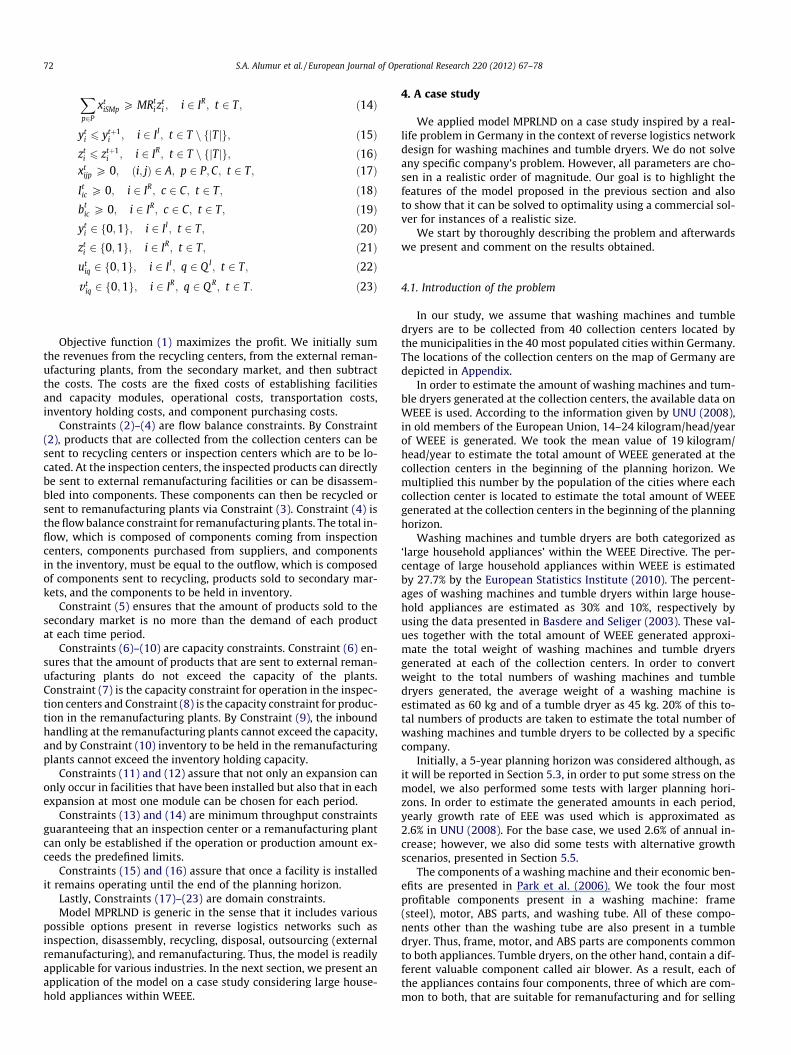
In the solution presented in Fig. 2, two inspection centers andtwo remanufacturing facilities are located each at Kassel and Ro-stock in the beginning of the first period. It is interesting to notethat the solution takes advantage of the possibility of co-locatinginspection centers and remanufacturing centers although no fixedcost incentive existed for that. This may be explained by the poten-tial savings in the transportation costs among these facilities.

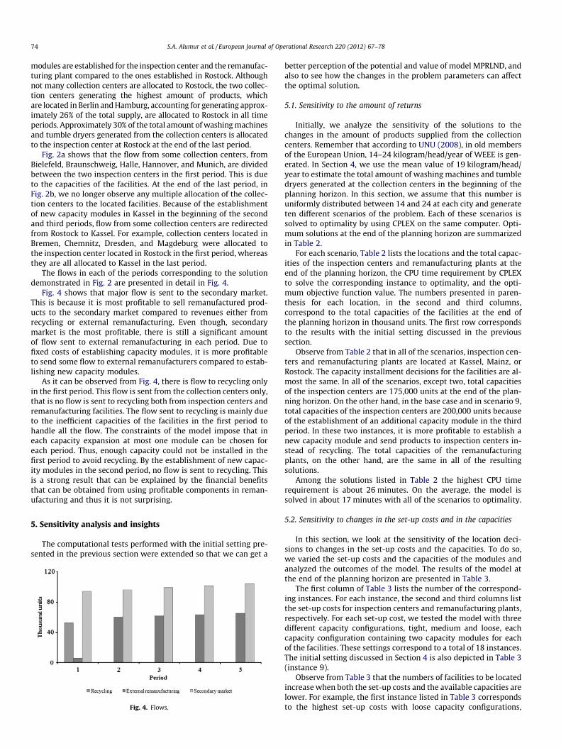
The capacity modules for the facilities are established within thefirst three time periods. Fig. 3 demonstrates the capacity installmentdecisions for all of the facilities at the end of each time period. In par-ticular, in the first period a ‘high’ capacity module is established forall of the located facilities. In the second period, a ‘high’ capacitymodule is established for the inspection center located at Kassel,and a ‘low’ capacity module for the inspection center located at Ro-stock. In addition, in the second period, a ‘low’ capacity module isestablished for the remanufacturing plant located at Kassel. In thethird period, only a ‘low’ capacity module is established for theinspection center at Kassel. The total final capacities of the inspec-tion centers located at Kassel and Rostock are 125,000 and 75,000units, respectively. On the other hand, the capacities of the remanu-facturing plants at the end of the planning horizon are 225,000 and150,000 units for Kassel and Rostock, respectively.

In Fig. 2a and b we can also observe the allocation of the collec-tion centers to the located inspection centers at the end of the firstand last periods. In all periods, most of the collection centers areallocated to the inspection center located in Kassel rather thanRostock. This is due to transportation costs, that is, Kassel is rela-tively closer to most of the collection centers compared to Rostock.In order to handle the incoming flow at Kassel, more capacity

74 S.A. Alumur et al. / European Journal of Operational Research 220 (2012) 67–78

modules are established for the inspection center and the remanufac-turing plant compared to the ones established in Rostock. Althoughnot many collection centers are allocated to Rostock, the two collec-tion centers generating the highest amount of products, whichare located in Berlin and Hamburg, accounting for generating approx-imately 26% of the total supply, are allocated to Rostock in all timeperiods. Approximately 30% of the total amount of washing machinesand tumble dryers generated from the collection centers is allocatedto the inspection center at Rostock at the end of the last period.

Fig. 2a shows that the flow from some collection centers, fromBielefeld, Braunschweig, Halle, Hannover, and Munich, are dividedbetween the two inspection centers in the first period. This is dueto the capacities of the facilities. At the end of the last period, inFig. 2b, we no longer observe any multiple allocation of the collec-tion centers to the located facilities. Because of the establishmentof new capacity modules in Kassel in the beginning of the secondand third periods, flow from some collection centers are redirectedfrom Rostock to Kassel. For example, collection centers located inBremen, Chemnitz, Dresden, and Magdeburg were allocated tothe inspection center located in Rostock in the first period, whereasthey are all allocated to Kassel in the last period.

The flows in each of the periods corresponding to the solutiondemonstrated in Fig. 2 are presented in detail in Fig. 4.

Fig. 4 shows that major flow is sent to the secondary market.This is because it is most profitable to sell remanufactured prod-ucts to the secondary market compared to revenues either fromrecycling or external remanufacturing. Even though, secondarymarket is the most profitable, there is still a significant amountof flow sent to external remanufacturing in each period. Due tofixed costs of establishing capacity modules, it is more profitableto send some flow to external remanufacturers compared to estab-lishing new capacity modules.

As it can be observed from Fig. 4, there is flow to recycling onlyin the first period. This flow is sent from the collection centers only,that is no flow is sent to recycling both from inspection centers andremanufacturing facilities. The flow sent to recycling is mainly dueto the inefficient capacities of the facilities in the first period tohandle all the flow. The constraints of the model impose that ineach capacity expansion at most one module can be chosen foreach period. Thus, enough capacity could not be installed in thefirst period to avoid recycling. By the establishment of new capac-ity modules in the second period, no flow is sent to recycling. Thisis a strong result that can be explained by the financial benefitsthat can be obtained from using profitable components in reman-ufacturing and thus it is not surprising.

5. Sensitivity analysis and insights

The computational tests performed with the initial setting pre-sented in the previous section were extended so that we can get a

Fig. 4. Flows.

better perception of the potential and value of model MPRLND, andalso to see how the changes in the problem parameters can affectthe optimal solution.

5.1. Sensitivity to the amount of returns

Initially, we analyze the sensitivity of the solutions to thechanges in the amount of products supplied from the collectioncenters. Remember that according to UNU (2008), in old membersof the European Union, 14–24 kilogram/head/year of WEEE is gen-erated. In Section 4, we use the mean value of 19 kilogram/head/year to estimate the total amount of washing machines and tumbledryers generated at the collection centers in the beginning of theplanning horizon. In this section, we assume that this number isuniformly distributed between 14 and 24 at each city and generateten different scenarios of the problem. Each of these scenarios issolved to optimality by using CPLEX on the same computer. Opti-mum solutions at the end of the planning horizon are summarizedin Table 2.

For each scenario, Table 2 lists the locations and the total capac-ities of the inspection centers and remanufacturing plants at theend of the planning horizon, the CPU time requirement by CPLEXto solve the corresponding instance to optimality, and the opti-mum objective function value. The numbers presented in paren-thesis for each location, in the second and third columns,correspond to the total capacities of the facilities at the end ofthe planning horizon in thousand units. The first row correspondsto the results with the initial setting discussed in the previoussection.

Observe from Table 2 that in all of the scenarios, inspection cen-ters and remanufacturing plants are located at Kassel, Mainz, orRostock. The capacity installment decisions for the facilities are al-most the same. In all of the scenarios, except two, total capacitiesof the inspection centers are 175,000 units at the end of the plan-ning horizon. On the other hand, in the base case and in scenario 9,total capacities of the inspection centers are 200,000 units becauseof the establishment of an additional capacity module in the thirdperiod. In these two instances, it is more profitable to establish anew capacity module and send products to inspection centers in-stead of recycling. The total capacities of the remanufacturingplants, on the other hand, are the same in all of the resultingsolutions.

Among the solutions listed in Table 2 the highest CPU timerequirement is about 26 minutes. On the average, the model issolved in about 17 minutes with all of the scenarios to optimality.

5.2. Sensitivity to changes in the set-up costs and in the capacities

In this section, we look at the sensitivity of the location deci-sions to changes in the set-up costs and the capacities. To do so,we varied the set-up costs and the capacities of the modules andanalyzed the outcomes of the model. The results of the model atthe end of the planning horizon are presented in Table 3.

The first column of Table 3 lists the number of the correspond-ing instances. For each instance, the second and third columns listthe set-up costs for inspection centers and remanufacturing plants,respectively. For each set-up cost, we tested the model with threedifferent capacity configurations, tight, medium and loose, eachcapacity configuration containing two capacity modules for eachof the facilities. These settings correspond to a total of 18 instances.The initial setting discussed in Section 4 is also depicted in Table 3(instance 9).

Observe from Table 3 that the numbers of facilities to be locatedincrease when both the set-up costs and the available capacities arelower. For example, the first instance listed in Table 3 correspondsto the highest set-up costs with loose capacity configurations,

Table 2Solutions of the model at the end of the planning horizon with different scenarios for the amount of products generated.

Inspection centers Remanufacturing plants CPU time (s) Obj. Func.

Base case Kassel (125), Rostock (75) Kassel (225), Rostock (150) 1531.66 51,041,892.24Scen. 1 Mainz (100), Rostock (75) Mainz (225), Rostock (150) 920.50 51,509,241.55Scen. 2 Mainz (100), Rostock (75) Mainz (225), Rostock (150) 605.11 53,246,272.18Scen. 3 Kassel (100), Mainz (75) Kassel (225), Mainz (150) 1102.71 49,858,989.38Scen. 4 Mainz (100), Rostock (75) Mainz (225), Rostock (150) 1108.32 52,647,963.95Scen. 5 Mainz (100), Rostock (75) Mainz (225), Rostock (150) 603.63 53,269,410.71Scen. 6 Mainz (100), Rostock (75) Mainz (225), Rostock (150) 756.87 52,726,199.14Scen. 7 Mainz (100), Rostock (75) Mainz (225), Rostock (150) 1054.72 52,508,169.24Scen. 8 Kassel (100), Rostock (75) Kassel (225), Rostock (150) 1568.31 52,535,074.96Scen. 9 Mainz (100), Rostock (100) Mainz (225), Rostock (150) 797.34 52,456,893.12Scen. 10 Mainz (100), Rostock (75) Mainz (225), Rostock (150) 1243.49 53,712,708.51

Table 3Solutions of the model at the end of the planning horizon with varying set-up costs and capacity modules.

Instance number Set-up costs(thousand EUR)

Capacity modulesfor inspection(thousand units)

Capacitymodules forremanu.(thousand units)

Inspection center locations Remanufacturing plant locations CPU time (s)

Ins. Remanu. High Low High Low

1 600 1500 100 50 300 150 Kassel Kassel 2060.162 500 1250 100 50 300 150 Kassel Kassel 2541.283 400 1000 100 50 300 150 Kassel Kassel 2057.634 300 750 100 50 300 150 Kassel Kassel 2377.805 200 500 100 50 300 150 Kassel, Magdeburg Kassel 4312.606 100 250 100 50 300 150 Augsburg, Magdeburg, Oberhausen Oberhausen 18732.19

7 600 1500 50 25 150 75 Kassel, Rostock Kassel, Rostock 1523.858 500 1250 50 25 150 75 Kassel, Rostock Kassel, Rostock 2031.899 400 1000 50 25 150 75 Kassel, Rostock Kassel, Rostock 1531.66

10 300 750 50 25 150 75 Mainz, Rostock Mainz, Rostock 1587.8811 200 500 50 25 150 75 Magdeburg, Mainz, Oberhausen Magdeburg, Mainz 1511.8712 100 250 50 25 150 75 Magdeburg, Mainz, Oberhausen Magdeburg, Mainz 2237.39

13 600 1500 40 30 100 80 Kassel, Mainz, Rostock Kassel, Rostock 6604.7314 500 1250 40 30 100 80 Mainz, Oberhausen, Rostock Mainz, Rostock 4123.1615 400 1000 40 30 100 80 Kassel, Mainz, Rostock Kassel, Mainz, Rostock 6545.0216 300 750 40 30 100 80 Kassel, Mainz, Rostock Kassel, Mainz, Rostock 4379.1717 200 500 40 30 100 80 Magdeburg, Mainz, Oberhausen Magdeburg, Mainz, Oberhausen 6137.2518 100 250 40 30 100 80 Lübeck, Magdeburg, Mainz, Oberhausen Lübeck, Mainz, Oberhausen 5843.05

S.A. Alumur et al. / European Journal of Operational Research 220 (2012) 67–78 75

where only a single inspection center and a remanufacturingplant is located both in Kassel. In the last instance listed in Table3, on the other hand, with lower set-up costs and tighter capac-ities, four inspection centers and three remanufacturing plantsare located.

In all of the solutions presented in Table 3, remanufacturingplants are co-located with inspection centers. As mentioned before,this can be explained by the potential savings from transportationcosts among these facilities.

In general, the model is solved in reasonable CPU time to opti-mality by CPLEX. The minimum CPU time requirement for themodel is about 25 minutes, whereas the maximum is about5.2 hours. Observe from Table 3 that the last set of instances withtight capacity configuration (instances 13–18) are relatively harderin terms of CPU time requirements.

5.3. The value of the multi-period model and the length of the planninghorizon

One important aspect to be analyzed concerns the potentialbenefits for the company of using the proposed 5-year model,rather than utilizing a static model. Our aim is to find whetherthe company will achieve additional profits by using the proposedmulti-period model.

For this analysis, we compared the profit performanceof a single-period model with that of the multi-period model overthe 5-year profit horizon on the 18 instances listed in Table 3.

Initially, we solved a single-period model using the average val-ues for the parameters over the entire planning horizon. Then, wefixed the locations and capacities throughout the planning horizonusing the solution of the single-period model and calculated theprofit that the firm can generate over the five years without alter-ing this network configuration. The results are presented in Table 4and Fig. 5.

The first column in Table 4 lists the instance numbers corre-sponding to the instances depicted in Table 3. The second columnpresents the optimal objective function value of the 5-period mod-el proposed in this study. The third column, on the other hand, pre-sents the total profits that the company will gain if the networkconfiguration of the 1-period solution using the average valuesfor the parameters over the entire planning horizon is fixed forthe 5-year planning horizon. Last column lists the percent differ-ences between the total profits.

In most of the solutions presented in Table 4, the total gain inthe profits by using the 5-period model are around 2%. Eventhough this percentage may seem as low, the potential signifi-cance is high since overall profits are high. If the total profitsare taken approximately as 50 million Euros, 2% corresponds to1 million Euros.

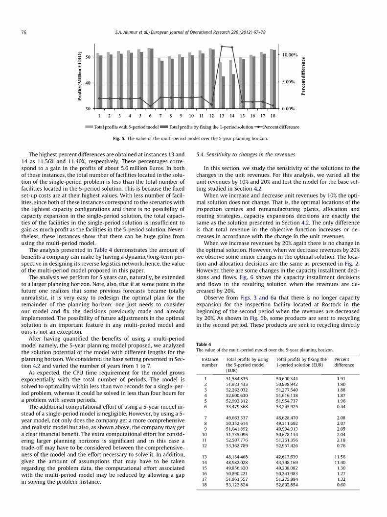
Table 4The value of the multi-period model over the 5-year planning horizon.

Instancenumber

Total profits by usingthe 5-period model(EUR)

Total profits by fixing the1-period solution (EUR)

Percentdifference

1 51,584,835 50,600,344 1.912 51,923,433 50,938,942 1.903 52,262,032 51,277,540 1.884 52,600,630 51,616,138 1.875 52,992,312 51,954,737 1.966 53,479,368 53,245,925 0.44

7 49,663,337 48,628,470 2.088 50,352,614 49,311,692 2.079 51,041,892 49,994,913 2.05

10 51,735,096 50,678,134 2.0411 52,507,776 51,361,356 2.1812 53,362,789 52,957,426 0.76

13 48,184,468 42,613,639 11.5614 48,982,028 43,398,169 11.4015 49,856,320 49,208,082 1.3016 50,890,221 50,241,983 1.2717 51,963,557 51,275,884 1.3218 53,122,824 52,802,854 0.60

Fig. 5. The value of the multi-period model over the 5-year planning horizon.

76 S.A. Alumur et al. / European Journal of Operational Research 220 (2012) 67–78

The highest percent differences are obtained at instances 13 and14 as 11.56% and 11.40%, respectively. These percentages corre-spond to a gain in the profits of about 5.6 million Euros. In bothof these instances, the total number of facilities located in the solu-tion of the single-period problem is less than the total number offacilities located in the 5-period solution. This is because the fixedset-up costs are at their highest values. With less number of facil-ities, since both of these instances correspond to the scenarios withthe tightest capacity configurations and there is no possibility ofcapacity expansion in the single-period solution, the total capaci-ties of the facilities in the single-period solution is insufficient togain as much profit as the facilities in the 5-period solution. Never-theless, these instances show that there can be huge gains fromusing the multi-period model.

The analysis presented in Table 4 demonstrates the amount ofbenefits a company can make by having a dynamic/long-term per-spective in designing its reverse logistics network, hence, the valueof the multi-period model proposed in this paper.

The analysis we perform for 5 years can, naturally, be extendedto a larger planning horizon. Note, also, that if at some point in thefuture one realizes that some previous forecasts became totallyunrealistic, it is very easy to redesign the optimal plan for theremainder of the planning horizon: one just needs to considerour model and fix the decisions previously made and alreadyimplemented. The possibility of future adjustments in the optimalsolution is an important feature in any multi-period model andours is not an exception.

After having quantified the benefits of using a multi-periodmodel namely, the 5-year planning model proposed, we analyzedthe solution potential of the model with different lengths for theplanning horizon. We considered the base setting presented in Sec-tion 4.2 and varied the number of years from 1 to 7.

As expected, the CPU time requirement for the model growsexponentially with the total number of periods. The model issolved to optimality within less than two seconds for a single-per-iod problem, whereas it could be solved in less than four hours fora problem with seven periods.

The additional computational effort of using a 5-year model in-stead of a single-period model is negligible. However, by using a 5-year model, not only does the company get a more comprehensiveand realistic model but also, as shown above, the company may geta clear financial benefit. The extra computational effort for consid-ering larger planning horizons is significant and in this case atrade-off may have to be considered between the comprehensive-ness of the model and the effort necessary to solve it. In addition,given the amount of assumptions that may have to be takenregarding the problem data, the computational effort associatedwith the multi-period model may be reduced by allowing a gapin solving the problem instance.

5.4. Sensitivity to changes in the revenues

In this section, we study the sensitivity of the solutions to thechanges in the unit revenues. For this analysis, we varied all theunit revenues by 10% and 20% and test the model for the base set-ting studied in Section 4.2.

When we increase and decrease unit revenues by 10% the opti-mal solution does not change. That is, the optimal locations of theinspection centers and remanufacturing plants, allocation androuting strategies, capacity expansions decisions are exactly thesame as the solution presented in Section 4.2. The only differenceis that total revenue in the objective function increases or de-creases in accordance with the change in the unit revenues.

When we increase revenues by 20% again there is no change inthe optimal solution. However, when we decrease revenues by 20%we observe some minor changes in the optimal solution. The loca-tion and allocation decisions are the same as presented in Fig. 2.However, there are some changes in the capacity installment deci-sions and flows. Fig. 6 shows the capacity installment decisionsand flows in the resulting solution when the revenues are de-creased by 20%.

Observe from Figs. 3 and 6a that there is no longer capacityexpansion for the inspection facility located at Rostock in thebeginning of the second period when the revenues are decreasedby 20%. As shown in Fig. 6b, some products are sent to recyclingin the second period. These products are sent to recycling directly

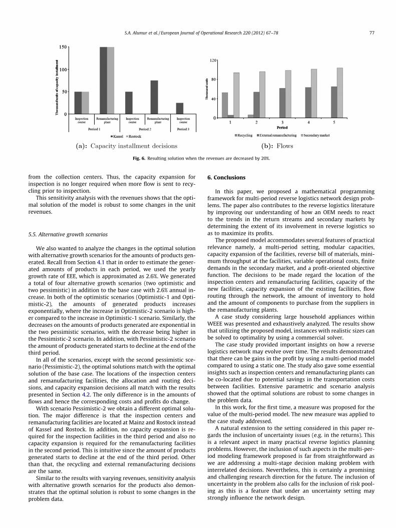
Fig. 6. Resulting solution when the revenues are decreased by 20%.

S.A. Alumur et al. / European Journal of Operational Research 220 (2012) 67–78 77

from the collection centers. Thus, the capacity expansion forinspection is no longer required when more flow is sent to recy-cling prior to inspection.

This sensitivity analysis with the revenues shows that the opti-mal solution of the model is robust to some changes in the unitrevenues.

5.5. Alternative growth scenarios

We also wanted to analyze the changes in the optimal solutionwith alternative growth scenarios for the amounts of products gen-erated. Recall from Section 4.1 that in order to estimate the gener-ated amounts of products in each period, we used the yearlygrowth rate of EEE, which is approximated as 2.6%. We generateda total of four alternative growth scenarios (two optimistic andtwo pessimistic) in addition to the base case with 2.6% annual in-crease. In both of the optimistic scenarios (Optimistic-1 and Opti-mistic-2), the amounts of generated products increasesexponentially, where the increase in Optimistic-2 scenario is high-er compared to the increase in Optimistic-1 scenario. Similarly, thedecreases on the amounts of products generated are exponential inthe two pessimistic scenarios, with the decrease being higher inthe Pessimistic-2 scenario. In addition, with Pessimistic-2 scenariothe amount of products generated starts to decline at the end of thethird period.

In all of the scenarios, except with the second pessimistic sce-nario (Pessimistic-2), the optimal solutions match with the optimalsolution of the base case. The locations of the inspection centersand remanufacturing facilities, the allocation and routing deci-sions, and capacity expansion decisions all match with the resultspresented in Section 4.2. The only difference is in the amounts offlows and hence the corresponding costs and profits do change.

With scenario Pessimistic-2 we obtain a different optimal solu-tion. The major difference is that the inspection centers andremanufacturing facilities are located at Mainz and Rostock insteadof Kassel and Rostock. In addition, no capacity expansion is re-quired for the inspection facilities in the third period and also nocapacity expansion is required for the remanufacturing facilitiesin the second period. This is intuitive since the amount of productsgenerated starts to decline at the end of the third period. Otherthan that, the recycling and external remanufacturing decisionsare the same.

Similar to the results with varying revenues, sensitivity analysiswith alternative growth scenarios for the products also demon-strates that the optimal solution is robust to some changes in theproblem data.

6. Conclusions

In this paper, we proposed a mathematical programmingframework for multi-period reverse logistics network design prob-lems. The paper also contributes to the reverse logistics literatureby improving our understanding of how an OEM needs to reactto the trends in the return streams and secondary markets bydetermining the extent of its involvement in reverse logistics soas to maximize its profits.

The proposed model accommodates several features of practicalrelevance namely, a multi-period setting, modular capacities,capacity expansion of the facilities, reverse bill of materials, mini-mum throughput at the facilities, variable operational costs, finitedemands in the secondary market, and a profit-oriented objectivefunction. The decisions to be made regard the location of theinspection centers and remanufacturing facilities, capacity of thenew facilities, capacity expansion of the existing facilities, flowrouting through the network, the amount of inventory to holdand the amount of components to purchase from the suppliers inthe remanufacturing plants.

A case study considering large household appliances withinWEEE was presented and exhaustively analyzed. The results showthat utilizing the proposed model, instances with realistic sizes canbe solved to optimality by using a commercial solver.

The case study provided important insights on how a reverselogistics network may evolve over time. The results demonstratedthat there can be gains in the profit by using a multi-period modelcompared to using a static one. The study also gave some essentialinsights such as inspection centers and remanufacturing plants canbe co-located due to potential savings in the transportation costsbetween facilities. Extensive parametric and scenario analysisshowed that the optimal solutions are robust to some changes inthe problem data.

In this work, for the first time, a measure was proposed for thevalue of the multi-period model. The new measure was applied tothe case study addressed.

A natural extension to the setting considered in this paper re-gards the inclusion of uncertainty issues (e.g. in the returns). Thisis a relevant aspect in many practical reverse logistics planningproblems. However, the inclusion of such aspects in the multi-per-iod modeling framework proposed is far from straightforward aswe are addressing a multi-stage decision making problem withinterrelated decisions. Nevertheless, this is certainly a promisingand challenging research direction for the future. The inclusion ofuncertainty in the problem also calls for the inclusion of risk pool-ing as this is a feature that under an uncertainty setting maystrongly influence the network design.

78 S.A. Alumur et al. / European Journal of Operational Research 220 (2012) 67–78

Acknowledgements

The authors appreciate the constructive criticism of two anon-ymous referees, whose feedback helped us in improving the paper.The first author is supported from the Scientific and TechnologicalResearch Council of Turkey (TÜB_ITAK); the third author is sup-ported by the Portuguese Science Foundation, POCTI – ISFL – 1 –152; the fourth author is supported by a team grant from the SocialSciences and Humanities research council of Canada.

Appendix A. Supplementary data

Supplementary data associated with this article can be found, inthe online version, at doi:10.1016/j.ejor.2011.12.045.

References

Aras, N., Boyacı, T., Verter, V., 2010. Designing the reverse logistics network. In:Ferguson, M., Souza, G. (Eds.), Closed Loop Supply Chains: New Developmentsto Improve the Sustainability of Business Practices. CRC Press, pp. 67–98.

Basdere, B., Seliger, G., 2003. Disassembly factories for electrical and electronicproducts to recover resources in product and material cycles. EnvironmentalScience Technology 37, 5354–5362.

Bleiwas, D., Kelly, T., 2001. Obsolete computers, ‘‘gold mine’’ or high-tech trash?Resource recovery from recycling. Fact Sheet FS-060-01, US Department of theInterior, US Geological Survey.

European Statistics Institute, 2010, <http://epp.eurostat.ec.europa.eu/portal/page/portal/eurostat/home/>.

European Union WEEE Directive, 2002, <http://eur-lex.europa.eu/LexUriServ/LexUriServ.do?uri=OJ:L:2003:037:0024:0038:EN:E>.

Figueiredo, J., Mayerle, S., 2008. Designing minimum-cost recycling collectionnetworks with required throughput. Transportation Research Part E 44, 731–752.

Fleischmann, M., Beullens, P., Bloemhof-Ruwaard, J., Van Wassenhove, L., 2001. Theimpact of product recovery on logistics network design. Production andOperations Management 10, 156–173.

Fonseca, M., García-Sánchez, A., Ortega-Mier, M., Saldanha-da-Gama, F., 2010. Astochastic bi-objective location model for strategic reverse logistics. TOP 18,158–184.

Gomes, M., Barbosa-Póvoa, A., Novais, A., 2011. Modelling a recovery network forWEEE: A case study in portugal. Waste Management 31, 1645–1660.

Jayaraman, V., Guide Jr., V.D.R., Srivastava, R., 1999. A closed-loop logistics modelfor remanufacturing. Journal of the Operational Research Society 50, 497–508.

Kanari, N., Pineau, J.-L., Shallar, S., 2003. End-of-life vehicle recycling in theEuropean Union. Journal of Operations Management 55, 15–20.

Krikke, H., van Harten, A., Schuur, P., 1999. Business case Oce: Reverse logisticsnetwork design for copiers. OR Spectrum 21, 381–409.

Krikke, H., Bloemhof-Ruward, J., Wassenhove, L.V., 2003. Concurrent productclosed-loop supply chain design with an application to refrigerators.International Journal of Production Research 41, 3689–3719.

Lee, D.-H., Dong, M., 2009. Dynamic network design for reverse logistics operationsunder uncertainty. Transportation Research Part E: Logistics and TransportationReview 45, 61–71.

Lieckens, K., Vandaele, N., 2007. Reverse logistics network design with stochasticlead times. Computers and Operations Research 34, 395–416.

Listes�, O., Dekker, R., 2005. A stochastic approach to a case study for productrecovery network design. European Journal of Operational Research 160, 268–287.

Louwers, D., Kip, B., Peters, E., Souren, F., Flapper, S., 1999. A facility locationallocation model for reusing carpet materials. Computers and IndustrialEngineering 36, 855–869.

Melo, M., Nickel, S., Saldanha-da-Gama, F., 2009. Facility location and supply chainmanagement – A review. European Journal of Operational Research 196, 401–412.

Park, P.-J., Tahara, K., Jeong, I.-T., Lee, K.-M., 2006. Comparison of four methods forintegrating environmental and economic aspects in the end-of-life stage of awashing machine. Resources, Conservation and Recycling 48, 71–85.

Pati, R., Vrat, P., Kumar, P., 2008. A goal programming model for paper recyclingsystem. Omega 36, 405–417.

Realff, M., Ammons, J., Newton, D., 2004. Robust reverse production system designfor carpet recycling. IIE Transactions 36, 767–776.

REVLOG, 1998. European Working Group on Reverse Logistics, <http://www.fbk.eur.nl/OZ/REVLOG/>.

Salema, M., Barbosa-Póvoa, A., Novais, A., 2009. A strategic and tactical model forclosed-loop supply chains. OR Spectrum 31, 573–599.

Salema, M., Barbosa-Póvoa, A., Novais, A., 2010. Simultaneous design and planningof supply chains with reverse flows: A generic modelling framework. EuropeanJournal of Operational Research 203, 336–349.

Sander, K., Schilling, S., Tojo, N., Van Rossem, C., Vernon, J., George, C., 2007. Theproducer responsibility principle of directive 2002/96/EC on waste electricaland electronic equipment (WEEE). <http://ec.europa.eu/environment/waste/weee/pdf/final_rep_okopol.pdf>.

Schultmann, F., Engels, B., Rentz, O., 2003. Closed-loop supply chains for spentbatteries. Interfaces 33, 57–71.

Srivastava, S., 2008. Network design for reverse logistics. Omega 36, 535–548.UNU, 2008. Review of directive 2002/96/EC on Waste Electrical and Electronic

Equipment (WEEE). <http://ec.europa.eu/environment/waste/weee/pdf/final_rep_unu.pdf>.