Multi-Objective versus Single-Objective Models in Geodetic ... · 8 Multi-Objective versus Single-Objective Models in Geodetic Network Optimization requirement of the network is satisﬁ

Nordic Journal of Surveying and Real Estate Research Volume 6, Number 1, 2009

Nordic Journal of Surveying and Real Estate Research 6:1 (2009) 7–20submitted on January 15, 2008

revised on June 21, 2008accepted on July 28, 2008

Multi-Objective versus Single-Objective Models in Geodetic Network Optimization

M. Bagherbandi, M. Eshagh, and L. E. SjöbergRoyal Institute of Technology, SE 10044, Stockholm, Sweden

[email protected]@kth.se

sjö[email protected]: +46 8 7907369; fax: +46 8 7907343

Abstract. Confi guration of a network and observation weights plays an important role in designing and establishing a geodetic network. In this paper, we consider single- and multi-objective optimization models in some numerical investigation. The results illustrate that the reliability model yields the best results in view of internal and external reliability and achievable observation precision. This result we interpret as that the reliability criterion is more sensitive to the confi guration of a network than any of the other criteria. We propose re-optimization of the network in the cases where very high (non-achievable) precision is required or when some conditions are not met in the optimization process.

Keywords: Optimization, analytical method, geodetic network, confi guration, weight.

Introduction1 An optimal geodetic network is a network having high precision and reliability designed according to economical considerations. The fi rst step of the geodetic network design is zero order design (ZOD) or datum defi nition. The datum affects the precision of the network too. Different criteria exist for selecting the best datum (ZOD). Teunissen (1985) presented the ZOD according to the theory of generalized matrix inverses and its relations with datum and rank defi ciency of the design matrix. Kuang (1996) presented different criteria for ZOD, and Eshagh (2005) suggested the minimum norm and trace of the co-factor matrix as the best criteria for datum defi nition.

There are two well-known ways to fi nd the best confi guration of networks, i.e., fi rst order design (FOD). One can use either the trial and error or the analytical approaches. In the trial and error method, the objective function (OF) is computed with a proposed solution for the problem. If the suggested solution does not satisfy the OF, the solution is changed and the OF is computed again. This process is repeated until the requirement is satisfi ed. The analytical approaches take advantage of a mathematical algorithm and design the network in such a way that the quality

8 Multi-Objective versus Single-Objective Models in Geodetic Network Optimization

requirement of the network is satisfi ed. A pioneer in using optimization theory was Koch (1982, 1985) who considered quadratic programming [Bazaraa and Shety, 1979] to optimize the confi guration of a network. Kuang (1991, 1996) developed this approach further and considered different types of optimization methods.

Grafarend (1975) and Schmitt (1980, 1985) presented different approaches for second order design (SOD) where SOD is optimal selection of the observables weights, and Kuang (1993) presented another approach to SOD leading to maximum reliability using linear programming [see e.g. Bazaraa (1974) or Smith et al. (1983)]. According to Eshagh (2005) numerical studies, the method of Kuang (1993) yields better results in SOD than other methods. Seemkooei (2001) considered the analytical approach to FOD, SOD and also their combinations in robustness points of view.

Using the method of Kuang (1996) one can obtain optimal weights and confi guration of the network in one step by different optimization algorithms and OFs. In fact, the approach proposed by Kuang (1996) to optimal design of the network is a combination of FOD and SOD. In this method the best confi guration and observation precisions are determined simultaneously in an optimal way. This optimal design can be carried out using different criteria as an OF. If just one criterion exists in the OF, it is called single-objective optimization model (SOOM); if two criteria exist, it is a bi-objective optimization model (BOOM) [Mehrabi 2002], and, if we have more than two criteria, we call it multi-objective optimization model (MOOM); see e.g. Kuang (1996). A simple comparison between different SOOMs has been carried out in Eshagh and Kiamehr (2007). This comparison shows that reliability is a much better criterion than the other criteria in SOOMs. The capability of the BOOM versus SOOM was presented in Eshagh (2005).

In this paper, after a quick review of SOOM and MOOM models, we compare them in a simple simulation study. The methodology is investigated for obtaining the optimum confi guration and observation weights considering the postulated reliability and precision requirements. The advantages and disadvantages of different SOOMs, such as precision, reliability and cost, as well as MOOM are presented and discussed. We investigate further the SOOM and MOOM and suggest the reliability model is better than the other SOOM and MOOM models for applying optimization of geodetic networks. The next section deals with a general review of the SOOMs and MOOMs and their mathematical models. In Section 3 we study these models numerically in a simple simulated network and compare the corresponding designs. The paper is ended by conclusions presented in Section 4.

Optimization models2 An optimum geodetic network should have an acceptable precision, high reliability and low cost. A general mathematical model for network optimization can be symbolically written by the following OF [Schaffrin, 1985]:

1 maxp r cα (precision)+α (reliability)+α (cost) =− (1)


where αp, αr and αc are parameters (weights) related to precision, reliability and cost, respectively. It is obvious that when one of these coeffi cients is zero, the model is a BOOM and if two coeffi cients are zero it becomes a SOOM. In the following we continue with different SOOMs.

2.1 Single Objective Optimization Models (SOOM)As mentioned before each one of the precision, reliability and cost criteria can be considered as an OF. Depending on which criterion that is regarded in the OF one can defi ne three different SOOMs. Each SOOM can be constrained to other quality factors. For instance, the precision criterion can be considered as the OF and the optimization is defi ned as a process to maximize the precision subjected to reliability and cost. Also, each SOOM can be subjected to two other controlling criteria. The main purpose of the analytical approach is to improve a primary design of the network. In this approach, the best possible confi guration (position shifts Δxi, Δyi, Δzi) and optimum observation weights (weight shifts Δpi) are sought. Some advantages of the analytical approach rather than other existing methods for network optimization are as follows:

Any type of geodetic observable can be considered. –Any condition or constraint can be considered. –All the criteria of precision, reliability and cost can be considered –simultaneously in the optimal design.The optimization procedure can be performed in the sense of FOD and SOD –separately or simultaneously.This methodology can be used for the optimal design of one-, two- or three- –dimensional networks.

In the following, three types of SOOMs are reviewed based on the criteria of precision, reliability and cost, respectively. We call such SOOMs precision, reliability and cost models, respectively.

2.1.1 Precision modelPrecision is the simplest criterion and that is well known. The variance-covariance matrix of the unknown parameters can be written in the general form:

( ) ( )1 120

T T T T TxC A PA DD E E DD E Eσ

− − = + − , (2)

where 20σ is a priori variance factor, P is the initial weight matrix, A is the network

confi guration matrix or the design matrix, D is the datum matrix including translation and rotation and scale parameters and E is the basis of the null space of the confi guration matrix A. The linearized form of Eq. (2) can be written:

0

1 1 1 1

m m m nx x x x

x i i i ii i i i

C C C CC C x y z px y z p

∂ ∂ ∂ ∂= + ∆ + ∆ + ∆ + ∆

∂ ∂ ∂ ∂∑ ∑ ∑ ∑x , (3)

where Δxi, Δyi, Δzi are unknown coordinate changes and Δpi are unknown corrections


to a priori weights. Equation (3) can also be represented in a vectorized matrix form as: Hw = u + ε, (4)where

( ) ( ) ( ) ( )01 1, , vec vecT T

u u u u x xH I I H u I I u C C= Θ = Θ = − , and (5)

( )1 1 1 1, , , , , , , , , Tm m m nw x y z x y z p p= ∆ ∆ ∆ ∆ ∆ ∆ ∆ ∆… … . (6)

In the above relations, ε is the residual vector making the system of equations Eq. (4) consistent, H is the coeffi cient matrix of the expansion including the derivatives of Cx with respect to the vector of unknowns w, u is a known vector since the approximate 0

xC and predetermined Cx are known, Θ is the Khatri-Rao product and vec is the converting operator of a matrix to vector; cf. e.g., Kuang (1996).

In fact, Eq. (4) presents a simple fi tting to a predetermined variance-covariance matrix (of required precision). The position and weight vector w changes until the best possible fi t to the required precision is met. The unknown w can be determined by using simple quadratic programming. In this case we may minimize the following relation:

2

minL

Hw u− → (7a)subject to:

H1w – u1 ≤ 0, (7b)

00 11 mr R w r+ ≥ , (7c)

mC C w c+ ≥00 11 , (7d)

0 0TD w = and (7e) A00w ≤ b00 , (7f)

where rm, cm are pre-defi ned redundancy number and weight boundary value. The matrices of H1, u1, r00, R11, C00 and C11 are related to precision, reliability and cost.

2L stands for L2-norm. For the details of computing these criteria, the interested readers are referred to Kuang (1996). Equations (7e) and (7f) are the datum constraints and shift limitation of unknowns; see also Kuang (1996).

2.1.2 Reliability modelReliability can also be considered as an OF to be maximized. Since in linear programming [Bazaraa 1974] the OF is minimized, this OF has to be considered with a minus sign. Such an OF is generally written as

( ) 1ˆˆ T T Tv l l A A PA DD A P I l Rl− = − = + − = −

, (8)

where v̂ is the residual vector of the system of observation equations. It differs from ɛ presented for the precision model. The Taylor expansion of Eq. (8) is:


0

1 1 1 1,

m m m n

i i i ii i i i

R R R RR R x y z px y z p∂ ∂ ∂ ∂

= + ∆ + ∆ + ∆ + ∆∂ ∂ ∂ ∂∑ ∑ ∑ ∑ (9)

where R0 is the redundancy matrix obtained from approximate a priori positions. Since we need just the diagonal elements of the redundancy matrix for our maximization problem, we can write the reliability criterion as

( )00 11 min

i Lr R w

∞

− + → , (10)where

( ) 0Tn nr I I r= Θ00 (11)

( )11 1,T

n nR I I R= Θ ( )0 0r vec R= , (12)

1

1 1 1

vec vec vec vec vm

R R R RRx y z x

∂ ∂ ∂ ∂= ∂ ∂ ∂ ∂

(13)

1

vec vec vec vec ,m m n

R R R Ry z p p

∂ ∂ ∂ ∂ ∂ ∂ ∂ ∂

and L∞is the L∞-norm. The above maximization problem can be summarized as:

( )00 11 mini L

r R w∞

− + → (14)

subject to: H1w – u1 ≤ 0, (14a) 00 11

T Tmc C w cγ γ+ ≤ , (14b)

0 0TD w = and (14c) A00w ≤ b00. (14d)

This problem can be solved by either linear programming or minimax programming. γ is a (3m + n) constant vector and the other parameters and constraints that have been introduced in the previous section. For details the reader is referred to Kuang (1996).

2.1.3 Cost modelCost may also be considered as the OF to be minimized. In the analytical design approach the number of repetitions of each individual observation can be a criterion for the cost. Such an OF is generally written as the target function for optimal cost in the network optimization:

L

P min∞→ . (15)

In the analytical approach by specifying approximate weights 0iP , we look

for the best possible improvements (ΔPi) for these weights as:


0i i iP = P + ΔP , (16)

where the weight improvement ΔPi is given by:

1

n

ii

PP Pp∂

∆ = ∆∂∑ . (17)

After linearization of the OF of Eq. (15) by using a Taylor series expansion we obtain the minimization problem of the cost:

00 11 minT Tc C wγ γ+ → (18a)

( ) ( )000 vecT

n nc I I P= Θ and (18b)

( ) ( )111

vec vec ,T Tn n n n

n

P PC I I I Ip p

∂ ∂= Θ Θ ∂ ∂

subject to: H1w – u1 ≤ 0, (18c) (r00 + R11w) ≥ rm , (18d)

0 0TD w = , and (18e)

A00w ≤ b00 . (18f)

Similarly, all parameters and constraints have been introduced in the previous section. Such model can be solved by using linear programming algorithms like simplex. For more details about linear programming the interested reader is referred to e.g. Baazara and Shety (1979).

2.2 Multi-objective optimization model (MOOM)As mentioned before, all SOOMs attempt to minimize or maximize a single OF describing the cost, precision or reliability. In practice there are constraints between each of the above criteria leading to inconsistencies in the optimization of the SOOM. To avoid such problems and lack of a unique minimum solution we can represent all OFs in one OF model [Kuang, 1996]:

( )

11 0011 00( )( )

minvec

T Tmm

m ms

C w c cHw u R w r rr cC

− −− − − + + →

γ γ (19)

subject to

0 0TD w = , and (20) A00w ≤ b00 . (21)

All parameters have been defi ned in the previous parts. Considering the L2-norm, Eq. (19) can be written as

0 0 0 0 0 02 minT T T Tw H H w u H w u u− + → , (22)


where

110

11

Ts s

Tm m

T

m

Hu uRHr r

Cc

=

γ

and

( ) ( )00

0

00

( )

( )

Ts s

mT

m m

Tm

m

u

vec C vec C

r rur r

c Cc

− = −

γ

, (23)

A11w ≤ b11, (24)

111

11

HA

R

= − and 1

1100 m

ub

r r

= − . (25)

Here w is the vector of unknown parameters as before, and u0 and H0 are known matrices.

Numerical studies3 A simple two dimensional geodetic network is considered for our numerical investigations. The network confi guration is presented in Figure 1. This network consists of 5 points having initial coordinates and all possible distances and angles as well as their initial weights are considered in the optimization problem.

5

800

1 00

0

1 20

0

1 40

0

1 60

0

1 80

0

2 00

0

2 20

0

2 40

0

2 60

0

2 80

0

3 00

0

1 000

1 200

1 400

1 600

1 800

2 000

2

3

14

Figure 1. The Network Confi guration.

Now, we should fi nd the best confi guration of the network as well as the best weights of observations according to the required quality. The standard error of 5 mm was considered as required precision of the position of net points. The network should be optimized in such a way that the redundancy of all observations is larger than rm = 0.6. The confi guration of the network is allowed to change


up to 3 m around each point during optimization process (–3 ≤ Δxi, Δyi, Δzi ≤ 3). The optimized observation weights are supposed to be positive and smaller than 1/(5 mm)2 for the distances and 1/(1.5 sec) (in radians) for angles with the initial values

i

0 2lP 1 (7mm)= and

i

0 2P 1 (2sec)α = (in radians), respectively. Before starting the optimization process let us determine the best datum of this network. As a criterion for fi nding the best datum for this network we have considered the minimum trace of the co-factor matrix. The best datum is defi ned when point 4 and the direction from point 4 to 2 are kept fi xed.

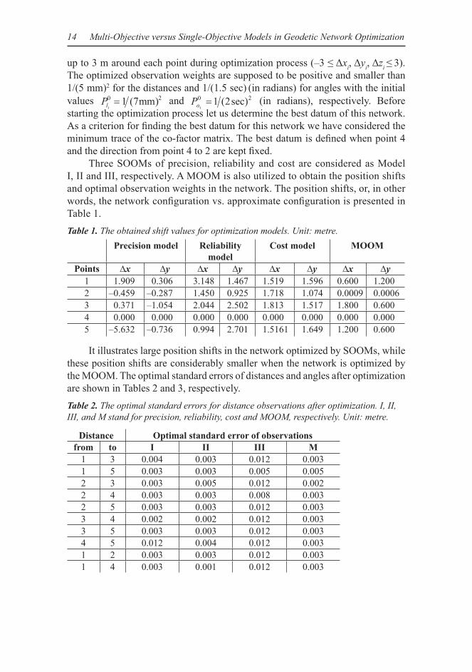
Three SOOMs of precision, reliability and cost are considered as Model I, II and III, respectively. A MOOM is also utilized to obtain the position shifts and optimal observation weights in the network. The position shifts, or, in other words, the network confi guration vs. approximate confi guration is presented in Table 1.Table 1. The obtained shift values for optimization models. Unit: metre.

Precision model Reliability model

Cost model MOOM

Points ∆x ∆y ∆x ∆y ∆x ∆y ∆x ∆y1 1.909 0.306 3.148 1.467 1.519 1.596 0.600 1.2002 –0.459 –0.287 1.450 0.925 1.718 1.074 0.0009 0.00063 0.371 –1.054 2.044 2.502 1.813 1.517 1.800 0.6004 0.000 0.000 0.000 0.000 0.000 0.000 0.000 0.0005 –5.632 –0.736 0.994 2.701 1.5161 1.649 1.200 0.600

It illustrates large position shifts in the network optimized by SOOMs, while these position shifts are considerably smaller when the network is optimized by the MOOM. The optimal standard errors of distances and angles after optimization are shown in Tables 2 and 3, respectively.Table 2. The optimal standard errors for distance observations after optimization. I, II, III, and M stand for precision, reliability, cost and MOOM, respectively. Unit: metre.

Distance Optimal standard error of observationsfrom to I II III M

1 3 0.004 0.003 0.012 0.0031 5 0.003 0.003 0.005 0.0052 3 0.003 0.005 0.012 0.0022 4 0.003 0.003 0.008 0.0032 5 0.003 0.003 0.012 0.0033 4 0.002 0.002 0.012 0.0033 5 0.003 0.003 0.012 0.0034 5 0.012 0.004 0.012 0.0031 2 0.003 0.003 0.012 0.0031 4 0.003 0.001 0.012 0.003


Table 3. The optimal standard errors for angles observations. I, II, III, and M stand for precision, reliability, cost and MOOM, respectively. Unit: sec.

Angles Optimal standard errors (sec)

st from to I II III M1 4 5 0.58 0.89 1.63 0.891 4 3 0.9 0.64 1.63 1.632 3 4 0.69 0.55 1.63 0.892 5 3 1.15 0.66 1.63 0.573 1 4 1.60 0.76 1.63 0.843 1 5 0.78 0.98 1.63 N/A3 5 2 0.67 0.65 1.63 N/A4 5 1 0.68 0.89 1.63 0.694 5 2 0.90 0.51 1.63 0.684 5 3 0.62 0.86 1.63 0.895 3 4 0.58 0.65 1.63 0.685 1 4 0.87 0.58 1.63 0.515 2 1 0.67 0.89 1.63 0.51

According to the initial precision of distances (5 mm), one can observe that all optimal standard errors of the distances are satisfi ed in the precision model except for one observable. The reliability model seems to have good capability to preserve the required accuracy. As could be expected, the cost model is not as good with respect to accuracy as the models I and II. These results agree with those obtained by Eshagh (2005) and Eshagh and Kiamehr (2007). As we will see in Table 8 and Figure 2, there is no proper internal and external reliability for the cost model. The MOOM seems to be the most fl exible model, and, as one may observe, all standard errors of the positions are smaller than the requested accuracy (5 mm) in Table 7.

In Table 3 the standard errors of the angles are illustrated. The requested accuracy for the angles is 1 arc second. The precision model shows good agreements of the optimal precision with required accuracy except for two observables. A very bad result is seen in the cost model. As expected, the reliability model presents very good agreement with the considered accuracy. However, one observable has larger standard error than the requested accuracy in the multi-objective model. The optimal weights for some observations are unsuitable as they are too large and therefore the observation variances are zero or close to zero. We know that observation weights are always assumed to be positive numbers. Now, after performing the optimization procedure, it is possible to see small weights for some observations yielding large standard deviations. On the other hand, it is of interest to have small weights to exclude unnecessary observations from optimization procedure. We use minimum and maximum bounds for the observable precision but some constraints are inconsistent even if we defi ne lower and upper bounds for them. The cost constraint is inconsistent with reliability and precision constraints, and then it violates some of the constraints. According to Table 3 we can neglect


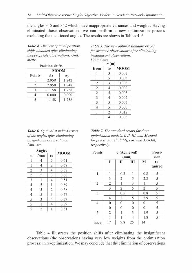
the angles 315 and 352 which have inappropriate variances and weights. Having eliminated those observations we can perform a new optimization process excluding the mentioned angles. The results are shows in Tables 4–6.

Table 4. The new optimal position shifts obtained after eliminating inappropriate observations. Unit: metre.

Position shiftsMOOM

Points ∆x ∆y 1 2.958 1.2422 2.958 1.8483 –1.158 1.7584 0.000 0.0005 –1.158 1.758

Table 5. The new optimal standard errors for distance observations after eliminating insignifi cant observations. Unit: metre.

σ (m)from to MOOM

1 3 0.0021 5 0.0032 3 0.0032 4 0.0022 5 0.0033 4 0.0023 5 0.0054 5 0.0051 2 0.0121 4 0.003

Table 6. Optimal standard errors of the angles after eliminating insignifi cant observations. Unit: sec.

Angles MOOMst from to1 4 5 0.611 4 3 0.682 3 4 0.582 5 3 0.683 1 4 0.514 5 1 0.894 5 2 0.684 5 3 0.575 3 4 0.575 1 4 0.895 2 1 0.51

Table 7. The standard errors for three optimization models, I, II, III, and M stand for precision, reliability, cost and MOOM, respectively.

Points σ (Achieved)(mm)

Preci-sion re-

quiredI II III M

1 1 0.3 1 0.8 53 2 5 2.8 5

2 2 1 3 1 53 2 5 2 5

3 1 0.5 1 0.8 54 2 5 2.9 5

4 0 0 0 0 50 0 0 0 5

5 2 1 3 1.9 51 1 4 1.8 5

trace 17 9.8 25 14

Table 4 illustrates the position shifts after eliminating the insignifi cant observations (the observations having very low weights from the optimization process) in re-optimization. We may conclude that the elimination of observations


causes larger position shifts in the network confi guration. Tables 5 and 6 show the optimal standard errors of the distance and angle observables. This study shows that the confi guration of the network changes considerably to satisfy the required precision. One can interpret these results as compensation of accuracy by changing the confi guration.

Table 7 shows the square roots of the diagonal elements of the variance-covariance matrix of the positions. The MOOM is the best after the reliability model. We experienced that the convergence of the optimization process based on MOOM takes more time versus the SOOMs. There is no inconsistency problem in optimization by MOOM, because all criteria are presented in one OF. Furthermore, for optimization of the network by using a SOOM we can vary the norm for minimizing or maximizing each single OF. All models satisfy the required precision (5 mm) in Table 7, but we have mentioned that reliability model has best internal and external reliability among all models. The cost model is inconsistent with precision and reliability conditions inferior vs. other models. Also Table 7 shows that the reliability model yields a smaller trace of the variance-covariance matrix than the other models and it agrees with precision and reliability constraints. Similarly we have the same situation as the precision model, but the OF is not similar to reliability and cost models. In the precision model the network is fi tted to the required precision in a least squares sense (based on L2 norm). In other words, we obtain the best fi t to the desired precision of network by changing the network confi guration and observations precision. In this case, the standard error of the positions is close to the desired one. Putting a precision constraint forces the optimization to deliver smaller error for the positions than the required one. However, in the reliability model the L∞ -norm is used so that it maximizes the minimum reliability of the network in the optimization procedure. In such

Table 8. Internal reliability for the three optimization models I, II, III, and M stand for precision, reliability, cost and MOOM, respectively.

Points Internal Reliability on the distances (mm)

from to I II III M1 4 0.006 0.002 0.006 0.0051 5 0.006 0.003 0.003 0.0062 3 0.007 0.005 0.009 0.0073 4 0.006 0.002 0.007 0.0052 4 0.007 0.004 0.016 0.0072 5 0.007 0.004 0.014 0.0061 3 0.007 0.003 0.008 0.0051 2 0.007 0.004 0.01 0.013 5 0.006 0.003 0.007 0.0074 5 0.012 0.006 0.01 0.01


a case, there is no fi tting to the residuals and the OF of reliability is maximized directly. The reliability model is quite consistent with precision condition as by increasing of reliability, the network tries to accept further observations. Thus, the position errors obtained from the least squares method (precision model) are decreasing when number of observations increase and reliability criterion satisfi es the precision requirements inherently. However there is no lower bound for the position errors in the reliability model, and they are minimized as much as possible while in the precision model the errors are delivered smaller but close to the required position errors. This is why the trace of variance-covariance matrix and position shifts due to the reliability model are smaller and larger than the precision model, respectively.

The absolute error ellipses for all fi ve network points after performing optimization by SOOMs and MOOM are presented in Table 9.Table 9. Absolute error ellipses for all optimization models. a and b are the semi-major and the minor axes of the error ellipses. Unit: mm.

Points Before optimization After optimization

a b a bI II III M I II III M

1 29 18 3 2 5 3 1 0.3 1 0.82 38 28 4 2 5 2 1 1 1 0.83 30 25 4 2 5 3 1 0.4 1 0.74 0 0 0 0 0 0 0 0 0 05 27 18 2 1 4 2 1 0.7 3 2

The effect of the largest undetectable gross error on the estimated positions obtained in a least squares adjustment are presented in Figure 2 for the x- and y-parameters. It is obvious that the reliability model yields the smallest external reliability.

The fi gure illustrates the external reliability of each position component of the fi ve network points. As would be expected, a network having high internal reliability, as presented in Table 8 delivers small external reliability, too.

Figure 2. The comparison of external reliabilities for optimization models.

0

2

1

3

4

5

6

7

1 2 3 4 50

5

10

15

20

25

30

1 2 3 4 5Number of net points

Model III

Exte

rnal

relia

bilit

y in

X (m

m)

Model I

MOOM

Model II

Number of net points

Model III

Model IMOOM

Model IIExte

rnal

relia

bilit

y in

Y (m

m)


Conclusions4 Before any measurement campaign is started, the geodesist should know the goal and requirements of the geodetic network to be designed. As is obvious, the highest precision and reliability of a geodetic network are expected, if all the observations are measured with highest accuracy. Since time and cost limitations do not allow extreme quality of a network, an optimum survey planning has to be made to achieve some prescribed design criteria with minimum effort. The main purpose is therefore to select the best datum, confi guration and suitable precision for observations for satisfying client criteria. In this paper single- and multi-objective optimization models were reviewed. The models were applied in a simple geodetic network to illustrate their performance. Numerical results show that the best SOOM is Model II (reliability model), maximizing the internal reliability. On the other hand, the reliability model also yields the best results in precision. The numerical results show that the reliability model delivers larger confi guration changes than the other SOOMs. It means that the initial confi guration was not well fi tted to the reliability model. It could also suggest that reliability is a more sensitive criterion to confi guration than any of the other OFs. In some cases contradictions between constraints exist, and some of the constraints may not be met. However, as we showed, such a problem seldom happens in the reliability model. One way for overcoming such problems is to use the MOOM, by which the constraints would be fulfi lled simultaneously in the best way. The analytical solution of the geodetic network is one of the best methods to design a network in such a way that it becomes an optimum network. Sometimes in the optimization process some observations get unrealistic weights corresponding to very high precision and some of the requirements are not met. In such a case re-optimization of the network is suggested after deleting those observables. In our numerical studies the MOOM yielded such results and we re-optimized the network. It is interesting to see that after eliminating the observables having unrealistic weights and re-optimizing the network, we got larger position changes with respect to previous optimization. Also we found that optimization based on MOOM does not converge as fast as the reliability model.

ReferencesBazaraa, M. S. (1974). Linear programming. J. Wiley and Sons Ltd, United States of America, New York.

Bazaraa, M. S. and C. M. Shetly (1979). Non-linear programming. J. Wiley and Sons Ltd, United States of America, New York.

Eshagh, M. (2005). Optimization and design of geodetic networks, Ph.D. study report in geodesy, Royal Institute of Technology, Division of Geodesy, Stockholm, Sweden.

Eshagh M. and Kiamehr R. (2007). A Strategy for Optimum Designing of the Geodetic Networks from the Cost, Reliability and Precision Views, Acta Geophysica et Geodaetica Hungaria, Vol 42: 297–308.

Koch, K. R. (1982). Optimization of the confi guration of geodetic networks, Deutsche Geodaetische Kommission, B, 258/III, 82–89, Munich, 1982.


Koch, K. R. (1985). “First Order Design: Optimization of the confi guration of a network by introducing small position changes”, in Optimization and design of geodetic networks edited by Grafarend and Sansó. Springer: Berlin etc. pp. 56–73.

Grafarend, E. (1975). Second Order Design of Geodetic Nets, Z.Vermessungswesen 100, 158–168.

Kuang. S. L. (1991). Optimization and Design of Deformation Monitoring Scheme, Ph.D. dissertation. Dept. of Surveying Engineering Technical Report No. 157, University of New Brunswick, P.O.Box 4400, Fredericton, Canada, July, 1991, 179 pp.

Kuang. S. L. (1993). “Second Order Design: Shooting for Maximum Reliability”, Journal of Surveying Engineering, Vol 119, No. 3, United States of America.

Kuang. S. L. (1996). Geodetic Network Analysis and Optimal Design: Concepts and Applications, ANN ARBOR PRESS, INC. 121 South Main Street, Chelsea, Michigan 48118, United States of America.

Mehrabi H. 2002: Fully analytical approach to bi-objective optimization and design of geodetic networks, MSc thesis, Department of Geodesy and Geomatics, K.N.Toosi University of Technology, Tehran, Iran.

Schaffrin, B. (1985). “Aspects of network design”, in Optimization and design of geodetic networks edited by Grafarend and Sansó. Springer: Berlin etc. pp. 548–597.

Schmitt, G. (1980). “Second Order Design of free distance networks considering different types of criterion matrices”. Bulletin Géodésique, 54 pp. 531–543.

Schmitt, G. (1985). “Second Order Design”, in Optimization and design of geodetic networks edited by Grafarend and Sansó. Springer: Berlin etc. pp. 74–121.

Smith, A. A, Hinton, E., Lewis, R. W. (1983). Civil Engineering Systems Analysis and Design. 3473. pp.. J. Wiley and Sons Ltd, London. Printed by page Bros Ltd, Norfolk.

Seemkooei, A. (2001). “Comparison of reliability and geometrical strength criteria in geodetic networks”, J. Geod., Vol. 75, Nr. 4 2001, pp. 227–233.

Teunissen, P. J. G. (1985), “Zero Order Design: Generalized inverses, Adjustment, the Datum problem and S-transformation”, in Optimization and design of geodetic networks edited by Grafarend and Sansó. Springer: Berlin etc. pp. 11–55.

Multi-Objective versus Single-Objective Models in Geodetic ... · 8 Multi-Objective versus Single-Objective Models in Geodetic Network Optimization requirement of the network is satisﬁ

Documents