MULTI-OBJECTIVE SLIDING MODE CONTROL OF ACTIVE …blog.uny.ac.id/mohkhairudin/files/2012/02/COMPLETE-THESIS.pdf · multi-objective sliding mode control of active magnetic bearing

MULTI-OBJECTIVE SLIDING MODE CONTROL OF ACTIVE MAGNETIC BEARING SYSTEM

ABDUL RASHID BIN HUSAIN

A thesis submitted in fulfilment of the

requirements for the award of the degree of

Doctor of Philosophy (Electrical Engineering)

Faculty of Electrical Engineering

Universiti Teknologi Malaysia

JULY 2009

ii

I declare that this thesis entitled “Multi-Objective Sliding Mode Control of Active

Magnetic Bearing System” is the result of my own research except as cited in the

references. The thesis has not been accepted for any other degree and is not

concurrently submitted in candidature of any other degree.

Signature : ………………………………

Name : ABDUL RASHID HUSAIN

Date : 23 JULY 2009

iii

DEDICATION To my dearest parents for their love and blessing.

To my dearly beloved wife, Norazah Abd Aziz for her support and encouragement.

To my son, Muhammad Ammar for making my life beautiful.

iv

ACKNOWLEDGEMENT

“In the name of Allah, The Most Gracious The Most Merciful”

I would like to express my sincere appreciation to my main supervisor Assoc. Prof. Dr. Mohamad Noh Ahmad for his guidance, supervision, advice and assistance in this research and preparation of this thesis. All the ‘teh tarik’ chats and discussions will definitely be one of the nicest memories to remember. My deepest gratituity also goes to my second supervisor, Prof. Ir. Dr. Abdul Halim Mohd. Yatim for his ideas especially during the initial stage of this research.

I am also very much indebted to Prof. Dr. Abdul Fatah Mohamad of Assiut

University, Egypt for helping and guiding me on the modeling of the Active Magnetic Bearing System and Dr. Tan Chee Pin of Monash University Malaysia for helping me in Sliding Mode Theory and Linear Matrix Inequality (LMI) when I first started. Also, I would like to thank Dr. Didier Henrion of LARS-CNRS, Toulouse, France for introducing me with the advance LMI materials and the LMI solver, YALMIP/SeDuMi, and Dr. Jiangfeng Zhang of University of Pretoria, South Africa for his very creative and nice explanation on linear system theory. I also would like to thank two gurus in Sliding Mode Control (SMC) theory, Prof. Okyay Kaynak of Bogazici University, Turkey and Dr. Christopher Edwards of University of Leicester, UK for very informative explanation of SMC and its research trend, and Prof. Ben Chen of National University of Singapore for sharing many of his knowledge on linear system theory. My appreciation also goes to Prof. Dr. Johari Halim Shah Osman for many informal discussions yet very fruitful.

I would like to thank my ‘phd-twin’, Sophan Wahyudi Nawawi for being my

research partner, Musa Mokji for giving many tips in using MATLAB, See Siew Min for the being the first person to introduce the LMI theory to me, and Tan Jo Lynn and Usman Ullah Sheikh for finding the ‘FOC’ journal articles.

I am also grateful to Universiti Teknologi Malaysia (UTM), my employer for

supporting this research in the form of scholarship and study leave. Last but never least, my beloved wife, Norazah Abd Aziz, for her love,

patience, understanding and unwavering support and to my wonderful son, Muhammad Ammar for cheering up my day.

v

ABSTRACT

Active Magnetic Bearing (AMB) system is known to inherit many nonlinearity effects due to its rotor dynamic motion and the electromagnetic actuators which make the system highly nonlinear, coupled and open-loop unstable. The major nonlinearities that are associated with AMB system are gyroscopic effect, rotor mass imbalance and nonlinear electromagnetics in which the gyroscopics and imbalance are dependent to the rotational speed of the rotor. In order to provide satisfactory system performance for a wide range of system condition, active control is thus essential. The main concern of the thesis is the modeling of the nonlinear AMB system and synthesizing a robust control method based on Sliding Mode Control (SMC) technique such that the system can achieve robust performance under various system nonlinearities. The model of the AMB system is developed based on the integration of the rotor and electromagnetic dynamics which forms nonlinear time varying state equations that represent a reasonably close description of the actual system. Based on the known bound of the system parameters and state variables, the model is restructured to become a class of uncertain system by using a deterministic approach. In formulating the control algorithm to control the system, SMC theory is adapted which involves the formulation of the sliding surface and the control law such that the state trajectories are driven to the stable sliding manifold. The surface design involves the transformation of the system into a special canonical representation such that the sliding motion can be characterized by a convex representation of the desired system performances. Optimal Linear Quadratic (LQ) characteristics and regional pole-clustering of the closed-loop poles are designed to be the objectives to be fulfilled in the surface design where the formulation is represented as a set of Linear Matrix Inequality optimization problem. For the control law design, a new continuous SMC controller is proposed in which asymptotic convergence of the system’s state trajectories in finite time is guaranteed. This is achieved by adapting the equivalent control approach with the exponential decaying boundary layer technique. The newly designed sliding surface and control law form the complete Multi-objective SMC (MO-SMC) and the proposed algorithm is applied into the nonlinear AMB in which the results show that robust system performance is achieved for various system conditions. The findings also demonstrate that the MO-SMC gives better system response than the reported ideal SMC (I-SMC) and continuous SMC (C-SMC).

vi

ABSTRAK

Sistem bearing magnet aktif (AMB) diketahui mempunyai pelbagai pengaruh kesan ketaklinearan disebabkan oleh pergerakan dinamik rotor dan penggerak sistem elektromagnet yang telah menyebabkan sistem ini mengalami ketaklinearan yang tinggi, terganding dan tidak stabil dalam kawalan gelung terbuka. Faktor penyumbang utama kepada ketaklinearan ini dikaitkan dengan kesan giroskopik, ketidakseimbangan berat rotor dan ketaklinearan elektromagnet di mana kesan giroskopik dan ketakseimbangan berat rotor adalah berkadar terus dengan kelajuan putaran rotor. Untuk mendapatkan sambutan sistem yang memuaskan dalam julat operasi sistem yang luas, kawalan aktif adalah diperlukan. Tesis ini membincangkan permodelan sistem AMB yang tak linear dan pembangunan pengawal tegap berasaskan kawalan ragam gelincir (SMC) di mana sistem yang dikawal akan mencapai prestasi tegap dalam pelbagai ketaklinearan sistem. Model AMB yang dibangunkan ini adalah berdasarkan integrasi antara dinamik rotor dan elektromagnet. Persamaan tak linear tersebut adalah berubah dengan masa dan persamaan ini mewakili penghampiran kepada ciri sistem yang sebenar. Berdasarkan kepada batasan parameter sistem yang diketahui, model ini distrukturkan semula menjadi satu kelas sistem tak pasti menggunakan pendekatan secara deterministik. Dalam membangunkan algoritma kawalan untuk mengawal sistem tersebut, teori kawalan ragam gelincir telah digunakan di mana kaedah ini melibatkan rekabentuk permukaan gelincir dan juga pembangunan hukum kawalan yang boleh memastikan trajektori sistem terpacu ke arah permukaan gelincir yang stabil. Rekabentuk permukaan gelincir melibatkan penukaran sistem kepada satu bentuk berkanun khas di mana pergerakan gelincir boleh diwakilkan oleh perwakilan cembung yang merangkumi prestasi sistem yang dikehendaki. Kuadratik Linear (LQ) optimum dan kawasan gugusan kutub yang dihasilkan dari kawalan gelung tertutup adalah objektif-objektif yang perlu dipenuhi dalam rekabentuk permukaan gelincir di mana ianya boleh diwakili sebagai satu set permasalahan pengoptimuman Ketaksamaan Matrik Linear. Untuk rekabentuk hukum kawalan, satu pengawal ragam gelincir berterusan yang baru telah dicadangkan. Hukum kawalan ini dapat menjamin sistem trajektori sampai ke kawasan kestabilan asimptot dalam satu masa yang terhingga. Ini dapat dicapai dengan menggunakan teknik kawalan setara yang digabungkan dengan lapisan sempadan yang menurun secara eksponen. Permukaan gelincir dan hukum kawalan yang baru dibangunkan ini membentuk pengawal kawalan ragam gelincir berbilang objektif (MO-SMC) lengkap. Pengawal ini kemudian diaplikasikan kepada sistem AMB tak linear di dalam pelbagai keadaan dan prestasi sistem secara tegap telah terbukti tercapai. Penemuan ini juga menunjukkan bahawa MO-SMC menghasilkan sambutan sistem yang lebih baik berbanding dengan teknik kawalan lain yang sedia ada iaitu kawalan ragam gelincir unggul (I-SMC) dan kawalan ragam gelincir berterusan (C-SMC).

vii

TABLE OF CONTENT

CHAPTER TITLE PAGE

DECLARATION ii

DEDICATION iii

ACKNOWLEDGEMENT iv

ABSTRACT v

ABSTRAK vi

TABLE OF CONTENTS vii

LIST OF TABLES x

LIST OF FIGURES xi

LIST OF SYMBOLS xv

LIST OF ABBREVIATIONS xxiii

LIST OF APPENDICES xxv

1 INTRODUCTION 1

1.1 Introduction to Active Magnetic Bearing (AMB)

System

1

1.2 AMB System Configurations and Control

Strategies

9

1.3 Summary of Existing Control Method for AMB

System

36

1.4 Research Objectives 37

1.5 Contributions of the Research Work 38

1.6 Structure and Layout of Thesis 39

viii

2 MODELLING OF ACTIVE MAGNETIC BEARING

SYSTEM

41

2.1 Introduction 41

2.2 Rotor Dynamic Model 42

2.3 Electromagnetic Equations 54

2.4 AMB System as an Integrated Model 55

2.5 AMB Model as Uncertain System 62

2.6 Summary 65

3 MULTI-OBJECTIVE SLIDING MODE CONTROL 67

3.1 Introduction 67

3.2 Problem Formulation 76

3.3 Multi-objective Sliding Surface 81

3.3.1 Optimal Quadratic Performance 82

3.3.2 Robust Constraint Pole-placement in

Convex LMI Region

89

3.3.3 Solution of Multiple Criteria using Convex

LMI

94

3.4 Sliding Mode Control Law Design 95

3.4.1 Fast-reaching Sliding Mode Design 96

3.4.2 Chattering Eliminations Using Continuous

Exponential Time-varying Boundary

Layer

100

3.5 The Proposed Controller Design Algorithm 103

3.6 Summary 106

4 SIMULATION RESULTS AND DISCUSSION 107

4.1 Introduction 107

4.2 Simulation Set-up and System Configuration 108

4.3 Simulation Results of the Multi-objective Sliding

Mode Control

112

ix

4.3.1 Multi-objective Sliding Surface 113

4.3.1.1 Effect of and Design

Matrices

114

4.3.1.2 Effect of Design Parameter, 139

4.3.1.3 Effect of Design Parameter,

, and

142

4.3.2 Surface Parameterization with Optimal

Quadratic Performance

144

4.3.3 Surface Parameterization with Robust

Constraint of Pole-placement in LMI

Region

147

4.4 The Effect of Design Parameter, , on System

Performance

150

4.5 The Effect of Design Parameter, and , on

Chattering Elimination

152

4.6 The Effect of Bias Current, Ib, on System

Performance

155

4.7 Comparison Between the Multi-objectives Sliding

Mode Controller with Ideal Sliding Mode

Controller and Continuous Sliding Mode

Controller

157

4.8 Summary 165

5 CONCLUSION AND SUGGESTIONS 167

5.1 Conclusion 167

5.2 Recommendation of Future Works 169

LIST OF PUBLICATIONS 171

REFERENCES 173

APPENDICES A-C 189-203

x

LIST OF TABLES

TABLE TITLE PAGE

1.1 Mode of operation for a pair of electromagnet 11

2.1 Parameters for AMB system 64

2.2 Range of state variables, input and rotor speed 64

4.1 Various values and the calculated H2 norm 139

4.2 Various c1 values and the calculated H2 norm 142

4.3 Calculated H2 norm and closed-loop eigenvalues for optimal

quadratic sliding surface

145

4.4 Closed-looped eigenvalues for sliding surface with robust

pole-placement constraint

148

4.5 and the power consumption index, Te 153

4.6 Bias current, Ib and power consumption index, Te 155

4.7 Maximum power consumption of AMB for MO-SMC,

I- SMC and C-SMC with the associated controller gains.

158

xi

LIST OF FIGURES

FIGURE TITLE PAGE

1.1 Active Magnetic Bearing System 3

1.2 Configurations of Active Magnetic Bearing System 4

1.3 Nonlinear relationship between magnetic force and

current/airgap

6

1.4 Illustration of unbalance rotor 7

1.5 Hardware configuration for closed-loop control of AMB

system

9

2.1 Cross section view of cylindrical horizontal AMB system

from x-z plane

43

2.2 Free-body diagram of AMB rotor 44

2.3 Movement of rotor in z-axis 52

3.1 Illustration of sliding that exists at intersection of two sliding

surfaces

68

3.2 States trajectory of third-order system given in (Choi, 1998) 69

3.3 Chattering phenomena due to infinite switching control law 70

3.4 LMI region for pole-placement 81

3.5 Representation of feedback system (3.36) 84

4.1 Singular value test of the system in original and transformed

coordinates

109

4.2 Flow charts of simulation preparations and set-up 112

4.3 Trajectories of X1 for parameter Set 1 116




xii

4.7 Rotor orbit for X1 vs. X3 (left bearing) for parameter Set 1 118


4.9 Control input for parameter Set 1 119




4.13 Sliding surface σ1 for parameter Set 1 121


























xiii







4.45 Trajectories of X1 (Varying ) 140

4.46 Control input (Varying ) 140

4.47 Sliding surface σ1 (Varying ) 141

4.48 Zoomed view of sliding surface σ1 141

4.49 Trajectories of X1 (Varying c1) 143

4.50 Control input (Varying c1) 143

4.51 Sliding surface σ1 (Varying c1) 144

4.52 Trajectories of X1 with optimal sliding surface 146

4.53 Control input with optimal sliding surface 146

4.54 Sliding surface σ1 with optimal sliding surface 147

4.55 Trajectories of X1 with LMI constraint pole-placement sliding

surface

148

4.56 Control input with LMI constraint pole-placement sliding

surface

149

4.57 Sliding surface σ1 with LMI constraint pole-placement sliding

surface

149







4.64 Trajectories of X1 (Varying Ib) 156

4.65 Rotor orbit for X1 vs. X3 (Varying Ib) 156

4.66 Trajectories of X1 of I-SMC, C-SMC and MO-SMC

( )

159

xiv


( )

159


( )

160


( )

160


( )

161

4.71 Control input of I-SMC, C-SMC and MO-SMC 161




4.75 Sliding surface σ1 of I-SMC, C-SMC and MO-SMC 163




xv

LIST OF SYMBOLS

SYMBOL DESCRIPTION

1. Upper case

effective cross-section area of the airgap

8×8 nominal system matrix of AMB system

, 8×8 system matrix of AMB system with current input

, 8×8 system matrix of AMB system with force input

ΔA(*,*) 8×8 uncertainty in system matrix of AMB system

generalized square matrix

8×8 transformed matrix,

( ( partitioned matrix

( partitioned matrix

( partitioned matrix

partitioned matrix

8×8 nominal linear dynamic matrix in new coordinate system,

8×4 nominal input matrix of AMB system

, , 8×4 input matrix of AMB system with current input

8×4 input matrix of AMB system with force input

nominal linear input matrix in new coordinate system,

coordinate transformation matrix,

∆ , , 8×8 uncertainty in input matrix of AMB system

4×4 state variable transformation matrix

xvi

design matrix related to

field of complex number

, , 8×1 disturbance vector

8×4 disturbance matrix

, , 8×1 disturbance vector containing the upper limit of each vector

element

design matrix related to

stable LMI region

stable LMI region region 1

stable LMI region region 2

steady-state airgap at equilibrium

, , continuous function related to ∆ , ,

, , continuous function related to , ,

4×1 force input vector

Fx net forces acting on the x-axis of stator frame

Fy net forces acting on the y-axis of stator frame

Fz net forces acting on the z-axis of stator frame

G Generalized feedback system dynamic

GXrYrZr moving rotor frame

G rotor center of geometry

Gm rotor center of inertia

, continuous function related to ΔA(*,*)

H2 energy in Hardy space

Ib bias current

Ic controlled current

Ii current in i-th coil

Imax maximum allowable coil current

LQ performance index

new LQ performance index related to output energy

Jx the moment of inertia around Xr

Jy the moment of inertia around Yr

controller parameter determining rate of reaching phase

K electromagnetic constant

xvii

linear controller gain,

transformed linear controller gain,

Lf moment of rotor around x-axis

surface design parameter

LMI block matrix

Mf moment of rotor around y-axis

slack matrix

N number of coil turn

Nf moment of rotor around z-axis

OXsYxZs static stator frame

O stator center of geometry

solution matrix for optimal quadratic surface

solution matrix for robust LMI region

partitioned matrix

partitioned matrix

symmetric positive definite matrix of state vector of LQ cost

function

partitioned matrix of

symmetric positive definite matrix of input vector of LQ

cost function

field of real number

design surface matrix

Sl linear sliding surface matrix

SPI proportional-integral sliding surface matrix

sliding surface matrix for I-SMC

sliding surface matrix for C-SMC

partitioned surface matrix of

partitioned surface matrix of

i-th sliding surface

i-th proportional-integral sliding surface

4×4 homogeneous transformation matrix of frame with respect to

frame 1

Transformation matrix into special regular form

xviii

3×3 simplified homogeneous transformation matrix

energy consumption index

Tm torque supplied by external motor

To the Coulomb friction torque

Tx torque around x-axis of stator frame

Ty torque around y-axis of stator frame

Tz torque around z-axis of stator frame

4×1 current input vector for AMB system

equivalent control term

ideal sliding mode control term

linear controller term

nonlinear controller term

exogenous disturbance

8×1 state vector for AMB system with current input

derivative of

4×1 desired state vector for AMB system with force input

matrix for LMI region

8×1 state vector for AMB system with force input

8×1 maximum value of state vector

transformed 8×1 state vector such that

i-th system state

i-th maximum value of system state

i-th initial system state

Xf force exerted on the rotor in x-axis

Xr x-axis of rotor frame coordinate

Xs x-axis of stator frame coordinate

system output vector

matrix for change of variable,

Yf force exerted on the rotor in y-axis

Yr y-axis of rotor frame coordinate

Ys y-axis of stator frame coordinate

output energy vector

Zf Force exerted on the rotor in z-axis

xix

Zr z-axis of rotor frame coordinate

Zs z-axis of stator frame coordinate

2. Lower case

ij-th element of the nominal matrix

, minimum and maximum bounds of ∆ , , respectively

∆ , ij-th element of the uncertain matrix ΔA(*,*)

ij-th element of the nominal matrix

, minimum and maximum bounds of ∆ , , , respectively

∆ , , ik-th element of the uncertain matrix ∆ , ,

upper limit of real value of eigenvalue in LMI region

lower limit of real value of eigenvalue in LMI region

4×1 disturbance force vector

maximum values of ∆ , ,

∆ , , i-th element of vector , ,

characteristic function of LMI region in complex plane

fdx disturbance force in x-direction

fdy disturbance force in y-direction

fdz disturbance force in z-direction

fdθ disturbance force around pitch angle

fdβ disturbance force around yaw angle

fex unknown external disturbance along x-axis

general electromagnetic force

electromagnetic coil of the ith coil

h electromagnet pole width

4×1 airgap deviation vector

gi airgap length

deviation of airgap

control current for horizontal left of rotor

control current for horizontal right of rotor

control current for vertical left of rotor

control current for vertical right of rotor

xx

electromagnetic constant

positive gain for relay-type control

negative gain for relay-type control

half of rotor length

mass of the rotor

mass of rotor imbalance

dimension of system input vector

dimension of system state vector

angular velocity components around Xr

angular velocity components around Yr

angular velocity components around Zr

bounds on the values ∆ , lis i-th linear sliding surface parameter

PIis i-th proportional-integral sliding surface parameter

bounds on the values

to initial time

reaching time of ideal sliding mode controller

reaching time of the new sliding mode controller

linear velocity components along Xr

linear velocity components along Yr

linear velocity components along Zr

xo initial state vector

x- coordinate of the rotor center relative to stator center

y- coordinate of the rotor center relative to stator center

z- coordinate of the rotor center relative to stator center

3. Greek symbol

matrix of boundary layer thickness for type switching

function

matrix of boundary layer thickness for continuous type switching

function

xxi

matrix of boundary layer thickness for exponential decaying type

switching function

state dependant switch gain matrix

controller design parameter determining reaching phase

sliding surface

sliding surface for C-SMC

sliding surface for I-SMC

, , design LMI region

design matrix for LMI region

design matrix for LMI region

design matrix for chattering elimination

Δ norm bound of continuous function ,

Δ norm bound of continuous function , ,

Δ norm bound of continuous function , ,

Π ij-th element of matrix

boundary layer thickness for C-SMC

design constant for chattering elimination

-th element of matrix

-th element of matrix

ς Angle of conical bearing

design parameter for convergence of exponential sliding surface

design parameter for optimized surface criterion

, , , lumped matched uncertainties

small positive constant for new sliding mode controller

small positive constant for ideal sliding mode controller

norm bound of lumped matched uncertainties

τ inertia inclining angle with respect to Xr (dynamic imbalance)

time variable

μo permeability of free space

κ initial angular values around pitch angle

ℓ bound of LQ performance index

λ initial angular values around yaw angle

eigenvalues of (*)

xxii

θ pitch angle

angle of the LMI region that specified damping factor of

closed-loop system

gain for continuous sliding mode controller

β yaw angle

ρ rotational angle (roll angle)

ζ torque damping coefficient

i-th airgap flux

radial distance of the unbalance mass from center of geometry

static imbalance

rotor radial eccentricity coefficient

rotor axial eccentricity coefficient

axial damping coefficient

xxiii

LIST OF ABBREVIATION

ADC Analog to Digital Converter

AMB Active Magnetic Bearing

CAC Current Almost Complementary

CCC Current Complementary Condition

CCS Constant Current Sum

CFS Constant Flux Sum

C-SMC Continuous Sliding Mode Control

CVS Constant Voltage Sum

DAC Digital to Analog Converter

DIA Disturbance and Initial-state Attenuation

DOF Degree of Freedom

DSP Digital Signal Processor

FEA Finite Element Analysis

FEM Finite Element Method

FL Fuzzy Logic

GA Genetic Algorithm

GEVP Generalized Eigenvalue Problem

IC Intelligent Control

I-SMC Ideal Sliding Mode Control

LDI Linear Differential Inclusion

LFT Linear Fractional Transformation

LMI Linear Matrix Inequality

LPV Linear Parameter Varying

LQ Linear Quadratic

LQR Linear Quadratic Regulator

xxiv

LSDP Loop Shaping Design Procedure

MO-SMC Multi-objective Sliding Mode Control

NN Neural Network

PD Proportional Derivative

PDD Proportional Derivative Derivative

PI Proportional Integral

PID Proportional Integral Derivative

PIDD Proportional Integral Derivative Derivative

SISO Single Input Single Output

SMC Sliding Mode Control

VSC Variable Structure Control

e.m.f Electromotive force

rpm Revolution per minute

xxv

LIST OF APPENDICES

APPENDIX TITLE PAGE

A Essential Theoretical Background 189

A1.1 Optimal State feedback Control 189

A1.2 H2 Norm and H2 Control 190

A1.3 Linear Matrix Inequality (LMI) 192

A1.3.1 LMI Problems 193

A1.3.2 Schur Complement 194

A1.3.3 LMI example 195

B LMI Solver 196

B1.1 Example: LQR for DC Motor Control and the

controller gains using ‘lqr’ and ‘are’ command

196

B1.2 LMI solution using LMI Toolbox 198

B1.3 LMI solution using Yalmip/SeDuMi 200

C Program of Multi-objective Sliding Surface and Control

Law

201

197

CHAPTER 1

INTRODUCTION 1.1 Introduction to Active Magnetic Bearing System

Bearings are one of the most essential components in all rotating machinery

and the study on its mechanism and development is becoming more indispensable as

the technology need pushes for more high-precision high-speed devices. By standard

definition, bearing is the static part of machine (stator) that supports the moving part

(rotor) of a system. While air and fluid bearings may be found in multi-degree-of-

freedom ball and socket joint of machines, ball bearings, which allow for pure

rotation, are by far the most popular and widely used in many industrial application

mainly due to its low production cost and ubiquitariness (Wilson, 2004). Magnetic

bearings are alternative to this traditional types or bearings, in which the bearings are

constructed from permanents magnets, electromagnets or both in which the bearing

in this combination is called hybrid magnetic bearing. An active magnetic bearing

(AMB) system is then defined as a collection of electromagnets used to suspend an

object via feedback control. For one degree-of freedom (DOF) system, usually AMB

is synonymously called magnetic suspension system as used in ground transportation

system where the vehicle is floated by the combination of controlled electromagnetic

and permanent magnetic forces i.e. Maglev Train (Trumper et al., 1997; Namerikawa

and Fujita, 2004; Fujita et al., 1998; Bleuler, 1992). For system with higher DOF,

AMB system contains a suspended cylindrical rotor that rotates in varying speed

depending on the applications. Thus, the obvious feature of AMB system is its non-

contact suspension mechanism, which offers many advantages compared to

conventional bearings such as lower rotating losses, higher operating speed,

2

elimination of high-cost lubrication system and lubrication contaminations,

suitability to operate at temperature extremes and in vacuum and having longer life

span (Okada and Nonami, 2002; Knospe and Collins, 1996; Bleuler, 1992). Due to

these significant reasons, AMB has been applied in a wide range of applications such

as industrial machineries and medical equipment, power and vacuum technologies,

and artificial heart, to quote a few applications (Knospe, 2007; Mohamed et al.,

1997b; Shen et al., 2000; Maslen et al., 1999, Tsiotras and Wilson, 2003; Kasarda,

2000; Lee et al. 2003).

Figure 1.1 illustrates an example of the standard structure of six-DOF AMB

system and the schematic arrangement of the rotor and magnetic coil (stator) of the

system. The system is composed of a cylindrical rotor or shaft made of laminated or

solid ferromagnetic material, sets of electromagnetic coils, power amplifiers, position

sensors and digital controller. The shaft is coupled to an external driving mechanism

such as pumps, electric motors or piezo actuators by a flexible coupling which

provides the rotational motion that forms the sixth DOF of the system. The

electromagnetic coils generate the magnetic forces by the current Ii and the position

sensors monitor the gap between the rotor and stator in which the captured

information is used by the digital controller to determine the control signal necessary

to suspend the rotating rotor to the centre of the actuating bearings. The control

signal is sent to the power amplifiers for necessary amplification of the current Ii

such that forces produced are able to withstand the dynamic requirement of the rotor

as well as the external mechanical load. In addition, with some changes in the

configurations of the AMB, the electromagnetic coils are not only able to supply the

radial forces, but also generate the forces for rotational motion consequently

eliminating the need of external driving mechanism. This so-called self-bearing

motor appears rather appealing for space-constraint application, however the design

construction and formulation of the control system is considerably much more

complex (Kasarda, 2000; Kanekabo and Okada, 2003; Bleuler, 1992).

3

(a) Typical AMB system set-up

(b) Rotor and electromagnetic coils (stator) with

respective coil currents, I1, I 2, I3 and I4.

Figure 1.1 Active Magnetic Bearing System

In most of AMB system, there exist separate sets of electromagnetic coils that

control the radial (x- and y- axes) and axial (z-axis) movement of the rotor due to

negligible dynamic coupling between these axes of motions. Advantageously,

Position sensors

Power supply cables

AMB for axial control

AMB for radial control

Rotor

Driving mechanism

(motor or pump)

I1

I3 I4

I2

Rotor

y

z x

y

x

4

separate control schemes are feasible to regulate the motions in radial and axial of

the system. As illustrated in Figure 1.1 (a), at each end of the rotor, a set of

electromagnetic coils is used for radial control where in each set, it contains two

pairs of coil as shown in Figure 1.1 (b). Based on this figure, at this end of the

system, the coil currents I1 and I2 supply the forces in y-direction while I3 and I4

supply the forces in x-direction. For the axial motion, one magnetic coil is located on

each side of the rotor end. As an alternative to electromagnetic coil, in some AMB

system where the rotor movement is very minimal, permanent magnets are sufficient

to supply the regulating axial force and thus more favored to be used.

(a) System with cylindrical AMB

(b) System with conical AMB

Figure 1.2 Configurations of Active Magnetic Bearing System

rotor

AMB for axial control


airgap, gi

Ii

Ii Ii

y

z

Ii


Ii

Ii Ii

Ii ς

airgap, gl

rotor

y

z

5

Figure 1.2 further illustrates two configurations of AMB system where in

Figure 1.2 (a), the cylindrical rotor is used. This is similar to the aforementioned

description of system in Figure 1.1 in which the axial motion is separately controlled

by a pair of electromagnetic coil. In contrast to this configuration, conical magnetic

bearing (Figure 1.2 (b)) where the rotor surface at the bearing end has small angle, ς,

which makes the airgap between the rotor and bearing to be in slanted position. With

this set-up, the electromagnetic coils supply both the axial and radial forces to the

system and the most obvious advantage obtained is the elimination of a pair of

axially-control electromagnetic coils. Nevertheless, this system experiences high

coupling effect between the axes and formulation of reliable controller under wide

operating is a very challenging task (Mohamed and Emad, 1992; Huang and Lin,

2004; Cole et al., 2004).

The various structural designs of AMB system are constructed to meet

different kind of requirements of the real-world application in order to exploit the

advantage of this non-contact lubrication-free technology. However, there are also

numerous nonlinearities inherited in AMB system that cause the system instability.

One of the most prominent nonlinearities is the relationship between the force-to-

current and force-to-airgap displacement. The general equation that governs the

magnetic force in AMB system is given as:

(1.1)

where μo is the permeability of free space, Ag is the cross-section area of the airgap,

N is the number of turn of the coil, and Ii and gi is the current and airgap at i-th coil,

respectively. By using the parameters given in (Mohamed and Emad, 1992; Lin and

Gau, 1997), this relationship can be plotted and shown in Figure 1.3 (a). Noticeably,

the relationship of the magnetic force in which the magnitude is proportional to the

square of the input current and inversely proportional to the square of the rotor

position causes sudden surge of the force magnitude as the airgap approaches zero.

Theoretically, this so-called negative stiffness imperatively causes singularity error

6

in many controller designs which practically translated to the saturation of magnetic

actuator. As one of the techniques to overcome this difficulty, a small bias current, Ib,

is usually introduced to the coil such that the linearity of the force-to-current about

(a) Nonlinear magnetic force

(b) Nonlinear magnetic force with biased current Ib = 0.8A

Figure 1.3 Nonlinear relationship between magnetic force and current/airgap

7

the centre of the system can be established to some degree which provides higher

system bandwidth and easier controller design. Figure 1.3 (b) shows the effect when

Ib = 0.8 A is added to the equation (1.1) where an almost linear relationship between

force and current and no singularity point is observed when the gap is zero.

Another major nonlinearity existed in AMB system is vibration due to the

mass unbalance of the rotor, or called imbalance. Imbalance is a common problem in

all machineries with rotational shaft when the principle axis of inertia of the rotor

does not coincide with its axis of geometry due to mechanical imperfections occurred

in fabricating machine parts, as shown in Figure 1.4 (Herzog et al. 1996; Shafai et al.

1994; Huang and Lin, 2004). When the rotor is ‘forced’ to rotate around its center of

inertia, Gm, instead of its centre of geometry, G, a centrifugal force caused by the

acceleration of the inertia centre creates a synchronous transmitted force and

furthermore manifested into synchronous rotor displacement. In the worst case

scenario, since the imbalance effect is proportional to the rotor rotational speed, at

high-speed operation the rotor whirls exceeding the allowable airgap and causes the

rotor to partially or worse yet annularly rub the stator which result in permanent

damage to the bearing system (Choi, 2002). Among the commonly considered

design solution to prevent this to occur is to have a mechanical retainer bearing

Figure 1.4 Illustration of unbalance rotor

x

ρ

y

Gτ

Gm

Stator

Rotor

8

installed as of the safety measures, however, the contact further exaggerates the

nonlinear dynamic motion to cause a more chaotic motion (Knospe, 2007; Grochmal

and Lynch, 2007; Li et al., 2006; Sahinkaya et al. 2004).

Other significant nonlinearities associated with the rotor dynamics are

gyroscopic effect and bending modes for flexible rotor. Gyroscopic effect present in

AMB system results in the coupling between the pitch (rotation around x-axis) and

yaw (rotation around y-axis) motion and the magnitude is proportional to the rotor

rotational speed. This imposes a more challenging task for stabilization of the system

for high-speed application (Li et al., 2006; Hassan, 2002). In addition, in some

applications where a long rotor is required, the excitation of flexible mode of the

rotor becomes crucial which may result in an inherently unstable system (Li et al.,

2006; Jang et al., 2005; Nonami and Ito, 1996).

In all AMB-related applications, the main objective is either asymptotically

regulating the rotor to center position (zero airgap deviation) of the system or

tracking a predefined rotor positions. However, with the presents of these

nonlinearities, the AMB system is liable to exhibit unpredictable and irregular

dynamic motions which complicate the design of effective system controller (Jang et

al. 2005, Kasarda, 2000). Conventional feedback controller methods developed by

assuming that the motions on each system axis are dynamically decoupled rarely

meet the stringent system requirements which result in limited operational range of

the system. Furthermore, nominal parameter values are commonly used in the system

where in real application, the exact values are poorly known and subjected to

variation which consequently result in deterioration of some controller performances

on the system. The need for more advanced control strategies is thus becoming

indispensable in order to achieve the desired system performance. In the following

section, the various control methods that have been designed for AMB system is

discussed.

9

1.2 AMB System Configuration and Control Strategies

The idea of active control magnetic bearing system has sparked interest as

early as 1842 after Earnshaw (1842) proved that the levitation of ferromagnetic body

and maintaining a stable hovering in six-DOF position is impossible to achieve by

solely using permanent magnet (Matsumura and Yoshimoto, 1986). Ever since then,

numerous control methods have been proposed by many research groups not only to

stabilize the system, but also to improve the performance of the system under

Figure 1.5 Hardware configuration for closed-loop control of AMB system

wide operational condition. Figure 1.5 illustrates the hardware set-up for the closed-

loop control of AMB system. The measurement of the four gap deviations forms as

the feedback information used by control algorithm executed in a fast Digital Signal

Processor (DSP) based processor. The calculated control signal is further amplified

to perform the required vibration control, positioning or alignment of rotor of the

system.

Gap sensors (Eddy current or

Hall-effect sensors)

AMB System

Low Pass filter

32 bit ADC High Speed DSP based

processor (Controller Algorithm)

32 bit DAC

Current/Voltage Amplifier

PC for logging

10

The electromagnets can be controlled by either the coil current (current-based

control) or the voltage (voltage-based control). In voltage-based control approach,

two design steps are usually adapted in which in the first step, a low-order current

controller is designed such that desired electromagnetic force is produced. Then,

tracking this current trajectory signal is used as the control objective for the design of

input voltage controller. The common assumption in this approach is the

combination of the processor and voltage amplifiers is able to fulfill the timing of the

two-stage nature of the controller which usually is very difficult to meet (Bleuler et

al., 1994b). Another important drawback is due to the inclusion of dynamic of the

power amplifier and circuit constraints, the linearization of amplifier and system

dynamics usually involved in the controller formulation which further limit the

system performance (Hassan, 2002; Charara et al. 1996). Some nonlinear control

methods such as differential flatness (Levine, et al., 1996), backstepping-type control

(DeQueiroz, et al. 1996a; DeQueiroz, et al. 1996b) and feedback linearization and

passivity-based control (Tsiotras and Arcak, 2005) are proposed but the difficulty of

overcoming singularity problem results in more complicated controller structures. In

the current-based control method, since there is a direct relationship between the coil

input current and the magnetic force shown by equation (1.1), the abovementioned

challenges in voltage-based control design can be relaxed and becomes more

advantages to AMB control system (Bleuler et al., 1994a).

The current-based control scheme can be classified into three modes of

operations of power amplifiers as shown in Table 1.1 (Sahinkaya and Hartavi, 2007;

Hu et al., 2004). The configuration of the tabulated coil currents is based on a single

pair of electromagnet in which one of the coils produces the opposite force of the

other coil. For Class-A control, a bias current, Ib, is applied to both coil and a

differential control current, Ic, is added to the bias current in one coil and subtracted

from the opposite coil depending on the net force required. The bias current is set to

half of the maximum allowable current, Imax. This mode of operation, also named as

Constant Current Sum (CCS) control, is the most widely used method in controlling

AMB system due to the fact that high bearing stiffness and good dynamic range can

be achieved (Grochmal and Lynch, 2007; Sahinkaya and Hartavi, 2007). In Class-B

mode of operation, or also known as Current Almost Complementary (CAC)

condition, a small bias current is supplied to both magnetic coils and at one instant of

11

Table 1.1 Mode of operation for a pair of electromagnet

Mode of Operations Input Current

Class A

,

,

where | | ,

0.5

Class B

and ,

or

and .

Class C

, 0,

or

0, ,

time, the control current is added to only one of the coils to produce the desired

control force. Although a possible lower power losses can be attained due to smaller

Ib, the bearing stiffness is reduced quite significantly which make the system to be

suitable for low vibration application. In this control mode, a possibly large feedback

gain is required to achieve the required bearing stiffness and likely will result in

current saturation. Tsiotras and Wilson (2003) and Tsiotras and Arcak (2005) have

shown that the control of AMB system with saturated input and low bias current is

nontrivial and a challenging nonlinear control problem. Another mode of operations

is the Class-C control where the bias current is totally eliminated and the two coils

are alternatively activated at an instant of time. This is equivalently called Current

Complementary Condition (CCC) where only one coil is energized depending on the

direction of the required force needed. Under this mode of operation, the nonlinearity

effects are severe and controller singularity problem occurred when the gap deviation

approaching zero is one of the most crucial design problems which result in

controller complexity. Apart from this design issue, the lacks of robustness against

changes in operating condition as well as poor dynamic performance are also major

shortcomings of this approach (Sahinkaya and Hartavi, 2007; Charara et al. 1996;

Levine et al. 1996).

12

Due to many possible combinations of design configurations and actuating

schemes exists in the control of AMB system, there exists abundance of control

design techniques that have been proposed to meet the control objectives which are

stabilization of the system and fulfilling specific application-related system

performances. The control strategies can be essentially divided into three main

groups: the linear control, nonlinear control and the control approach based on

mimicking human’s decision making process and reasoning or known as Intelligent

Control (IC) method. The linear and nonlinear control strategies are model-based

approaches where a mathematical model representing the AMB system as a class of a

dynamical system is a required for the development of the control. As an alternative,

due to the complexity in formulating the control law especially for the nonlinear

control techniques, the adaptation of the IC methods in AMB control has found

growing interest especially Fuzzy Logic (FL), Genetic Algorithm (GA) and Neural

Network (NN), or the fusion of any of the method with existing mathematical-based

methods.

The conventional Proportional-Derivative (PD), Proportional-Integral (PI)

and Proportional-Integral-Derivative (PID) control for AMB system are among the

earliest controllers considered for the control of AMB system due to its simplicity in

the design as well as hardware implementation (Bleuler et al., 1994b) and until

today, the controller still receives considerable attention in some specialized

application. In the work done by Allaire et al. (1989) and William et al. (1990),

discretized PD controller is designed based on linearized model at a nominal

operating point. The main emphasis of the work by Allaire et al. (1989), however, is

the design construction of AMB system to accommodate the variation of the load

capacity in thrust motion and the PD controller is used to achieve closed-loop

stability. Due to apparatus limitation, mechanical shims are used to gauge the airgap

and the controller is manually adjusted. William et al. (1990) has continued the study

where the relationship between the characteristic of the developed PD controller to

the stiffness and damping properties of AMB system is established. Other than

stiffness and damping curves, the rotor vibratory response is also used to show the

effectiveness of the control algorithm where from the experimental result, due to

time delay in feedback response and hardware limitation, the high frequency

response does not agree with the theoretical result. To overcome the difference, the

13

so-called Proportional-Derivative-Derivative (PDD) and Proportional-Integral-

Derivative-Derivative (PIDD) are proposed and applied into the system which yields

quite a satisfactory result.

In more recent year, Hartavi et al. (2001) has studied the application of PD

controller on 1 DOF AMB system where the electromagnetic model is developed

based on Finite Element Method (FEM), initially proposed by Antilla et al. (1998).

Good system stability is achieved, however, only under limited range of operating

condition. Polajzer et al. (2006) has further proposed a cascaded decentralized PI-PD

for control of the airgap and independent PI current controller to achieve high

bearing stiffness and damping effect of a four DOF AMB system. The controller is

designed based on simplified linearized single-axis model where the effect of

magnetic nonlinearities and cross-coupling effect are ignored. A considerable

improvement has been achieved in term of its static and dynamic response in

comparison to PID control developed in previous work. In an AMB system where

the rotor is flexible, the control of vibration due to bending mode of the rotor is

crucial. For the AMB system developed by Okada and Nonami (2002), a hybrid-type

magnetic bearing is used and PD controller is proposed to perform the inclination

control such that the system with flexible rotor is able to step through the bending

modes occurred at five critical rotational speeds. The five bending modes are

analyzed from the finite element model of the rotor that is transformed into a linear

state equation and the controller parameters are designed based on the linearized

model. With the central rotor position is controlled separately to provide sufficient

stiffness, the system with the proposed PD controller for inclination control is able to

run up to 6300 rpm rotational speed.

Due to limited performance of PD, PI or PID controller and design

procedure to incorporate various design requirements, other linear controller methods

have been proposed to fully exploit the possible active potentials of the AMB system

in permitting to a much higher degree of rotor vibration and position control (Bleuler

et al., 1994a; Huang and Lin, 2003). Another most popular linear control method

used by researchers is the Linear Quadratic Regulator (LQR) control which is based

on optimal control theory (Anderson and Moore, 1990). LQR design method is

designed by selecting the so-called weighting matrices that minimizes a pre-defined

14

linear quadratic cost function. Matsumura and Yoshimoto (1986) are considered as

among the earliest researchers that have applied the LQR-type controller in AMB

system. In their study, an LQR controller is designed and cascaded with and integral

term such that the steady-state error of the airgap deviation is eliminated. This

optimum servo-type control is formulated based on a linearized 5-DOF AMB system

at a constant biased current, where the deviations of rotor position from this

equilibrium are treated as system states to be regulated and the input to the system is

the electromagnetic voltages. The digital simulation results show that the system

achieve stability condition at zero speed and 90000 rpm, however, at this high

rotational speed, the coupling effect influence the control performance significantly.

The method is further applied into a system where the integral servo-type control is

to perform both the radial and thrust control for a cylindrical AMB system

(Matsumura et al., 1987). Through this study it is verified that multi-axial control of

AMB system is difficult to achieve with the proposed type of controller. Since both

of these works are based on a linearized model at one operating point, Matsumura et

al. (1999) has used a different linearization technique called exact linearization

approach such that the linear model can represent a wider range of the nonlinear

model. The design LQR controller for this newly linearized model confirms to

achieve wider range of stabilization area. The control method of this highly-cited

work (Matsumura and Yoshimoto, 1986) is also further adapted in a new type of

horizontal hybrid-type magnetic bearing (Mukhopadhyay et al. 2000). In this work,

the new type AMB system is developed by using a rotor made from strontium-ferrite

magnet and both the top and bottom stators are made from Nd-Fe-B material where

the combination of this permanent magnet configuration is proven to provide high

bearing stiffness to produce repulsive force for rotor levitation. The force-to-airgap

relationship is established by using finite element analysis (FEA) where the

relationship is integrated with the dynamic model of the AMB system. The optimum

integral servo-type control is designed to stabilize the system and tested on the

system up to the 800 rpm rotor speed.

In a quite similar scope of work, Lee and Jeong (1996) has designed

centralized and decentralized LQR controller with integrator to perform a control on

a vertical conical AMB system. For the centralized control, the coupling effect

between the axial and thrust motions is considered and this effect is ignored on the

15

decentralized controller design. The relationship between the current and voltage is

emphasized where the mathematical model of the electromagnetic coil dimension

and its dynamics are included in the design procedure where it is illustrated that the

coupling effect between the axial and radial axes of motion is quite insignificant for

the particular AMB system which result both the centralized and decentralized

controller produce comparatively similar performances. In a rather different

approach, Zhuravlyov (2000) has explored the design of LQR controller for not only

regulating the rotor position but also to reduce the copper losses in the coils. Two-

stage LQR based controller is developed such that the first controller is meant to

stabilize the rotor to the reference position with magnetic force is the system input.

For the second stage, another LQR controller is developed to produce the coil current

and voltage which produces the optimized bearing force while at the same time, the

copper losses in the coil is also minimized. Instead of taking the real value of the

system matrix, this approach has used the complex state-space system such that the

frequency content of the system can be incorporated. The study also shows that the

real implementation of the controller is difficult especially when the second stage

controller requires a switching term to achieve the desired objective, and controller

simplification is needed for practical purposes.

The works in the development of controller based on μ-synthesis have also

been reported by many researchers. Fujita et al. (1995) has proposed the μ-synthesis

controller that is designed based on a few set of active electromagnetic suspension

model. The combination of the nominal model, four set of model structures and

possible model parameter values are used to determine uncertainty weighting

function which form a sufficient representation of the range where the real system is

assumed to reside. A special so-called D-K iteration is then used to tune the

controller parameter to achieve robust stability as well as robust performance.

Nonami and Ito (1996) have used μ-synthesis method for stabilization of five-axis

control of AMB system with flexible rotor. The modeling of the system is performed

by using FEM technique and the resulted high order system is truncated by removing

the flexible mode for the purpose of controller design. It is shown that the controller

can achieve robust performance for this system and the it is noted that by value of the

structured singular value, µ, in the D-K iteration contribute to achieving good robust

performance.

16

Namerikawa and Fujita (1999) have further included more nonlinearities in

the AMB model by specifically classifying linearization errors, unmodelled

dynamics, parametric variations and gyroscopic effect as the uncertainties in the

system. These uncertainties are represented structurally in matrices and Linear

Fractional Transformation (LFT) technique is used to uniformly represent the AMB

as a class of uncertain system for controller development. Instead of using standard μ

test, a so-called mixed μ test is adapted to reduce the design conservatism. Losch et

al. (1999) have designed and implemented the μ-synthesis controller in a feed pump

boiler equipped with active magnetic bearings. They have proposed a systematic and

formalized way for deriving the controller design parameters based on model

uncertainties, control requirements and known system limitations. A new method for

determining suitable uncertainty weighting function has been proposed in which the

effectiveness of the designed controller is demonstrated by the robust performance of

the pump.

In different scope of research, Fittro and Knospe (2002) has designed the μ-

synthesis controller for specifically solve the rotor compliance minimization problem

– to reduce the maximum displacement that may occur at a particular rotor location

collocated at the region the disturbance frequency is not specified. Although the

controller produces a significant improvement compared to PD controller, the results

obtained however has suggested that a more accurate plant mode is required to yield

a more accurate result in minimizing the rotor compliance.

Another robust linear control design that has received considerable attention

in the control of AMB system is H∞ technique. Since the linear model does not

always express the exact representation of the system due to various uncertainties

present in the system, H∞ control technique offer a nice procedure to construct the

uncertainties into a proper structure for control design process. Fujita et al. (1990)

has worked on verifying the well-established H∞ controller on an experimental set-up

of a one DOF magnetic suspension system. The main objective is to achieve robust

system stabilization when the system is subjected to external disturbance. Various

model uncertainties are also considered by formulating frequency weighting function

which is included in the design procedure. Fujita et al. (1993) further develop H∞

controller for five DOF AMB system by using the Loop Shaping Design Procedure

17

(LSDP). The so-called unstructured multiplicative perturbation which describes the

plant uncertainties with the frequency weighting function is established which

reflects the magnitude of uncertainties present. After specifying the uncertainty and

performance weightings, by using the LSDP the shaping function is designed where

the H∞ controller is developed and tested experimentally which shows that some

minor online adjustment on the shaping functions is still required to achieve a more

favourable system response in term of regulating the airgap at various frequencies.

A simplified H∞ controller has been designed by Mukhopahyay et al. (1997)

for repulsive type magnetic bearing where an AMB configuration with permanent

magnet in the radial axis is used to increase the bearing stiffness. The result from the

study shows with the combination of the proper placement of the permanent magnet

and controller design the radial disturbance is able to be attenuated for an 8 kg non-

rotating rotor.

A continuous and discrete time H∞ controller have been proposed by Font et

al. (1994) to regulate the rotor to the center position of an electrical drive system by

using AMB. The first six bending modes of the rotor is included in the system model

such that the design controller can achieve robust stability towards the frequency

excitation occurred at these modes. For the continuous controller, instead of using

the truncated method, an aggregation method to reduce the order of the system is

adapted where this technique offers the advantage of retaining the most important

poles in the reduced order system. Satisfying closed-loop behaviors have been

obtained, however, the power amplifier introduces severe constraint on the control

capability.

Namerikawa and Fujita (2004) and Namerikawa and Shinozuka (2004) have

used the H∞ controller design technique for disturbance and initial-state attenuation

(DIA) on magnetic bearing and magnetic suspension system, respectively. In the

design procedure of the proposed H∞ DIA controller, the selections of the frequency

weighting related to the disturbance input, system robustness and the regulated

variables are performed iteratively for the construction of linearized generalized

system plant. A so-called weight matrix N obtained from this procedure is found to

indicate the relative importance between attenuation of disturbance and intial-state

18

uncertainty which further affects the calculated controller gains. Four H∞ DIA

controllers have been designed under different values of frequency weighting to

assess the variation of matrix N on the system performance where it is shown the

system overshoot is inversely proportional to the magnitude of N. In (Namerikawa

and Fujita, 2004), the non-rotational AMB is used which implies that no gyro-scopic

effect and imbalance present.

In a more recent work, Tsai et al. (2007) has proposed H∞ control design for

four-DOF vertical AMB system with gyroscopic effect. The well-known Kharitonov

polynomial and Nyquist Stability Criterion are employed for the design of the

feedback loop and it is confirmed experimentally that the controlled current produced

is much less compared to the current produced by LQR or PID control methods. The

performance of the system is verified in the range 6500 rpm to 13000 rpm rotor

rotational speed.

Linear controller based on Q-parameterization theory has also been widely

tested and applied in AMB system starting with the work from Mohamed and Emad

(1992). In this work, a Q-parameter controller based on linearized conical AMB

model is proposed which can meet various system requirements such as disturbance

rejection, rotor stability and tolerances towards plant parameter variations. In the

design procedure, these requirements are treated as constraints and can be classified

by the doubly co-prime factorization matrices and the sets of stabilizing controllers

which include the free design parameter Q. The search of the desired Q-parameter

that produces the desired controller gain becomes an optimization problem where

Q’s are chosen through a customized optimization program. In this work, the

controller is designed for imbalance-free rotor at speed p = 0, and good transient and

force response is achieved until p = 15000 rpm. Since the order of the controller

equal to the order of the plant and the order of the weighting function describing the

constraint, the works are further extended by Mohamed et al. (1997a) where the

linear system is transformed into three single-input-single-output (SISO) systems

with the inclusion of the rotor imbalance. This simplification results in solving a set

of linear equation rather that finding the solution from the complex optimization

problem, where good rotor stabilization is achieved at three pre-defined rotor speed.

19

The Q-parameterization controller in discrete form is proposed by Mohamed

et al. (1999) to specifically overcome the imbalance at various speed. The rotational

speeds are scheduled in a table and appropriate gain adjustment according to the

selected speed will be selected as the Q-parameter for the controller. This gain-

scheduling method shows the elimination of imbalance at three rotor rotational speed

is achieved with simpler design technique, however, a large look-up table is required

to accommodate the operation at wider range of rotor rotational speeds.

With the linearization of force-to-current and force-to-airgap displacement

relationship, AMB model belongs to a class of linear parameter varying (LPV)

system which is suitable for LPV controller design. Zhang et al. (2002) has proposed

a class of LPV controller that can maintain robust stability and performance at wide

range of rotor speed. The augmented AMB system model is characterized as many

sets of convex representation of system where the system matrix is considered as

affine function of the rotor speed and treated as a set of structured uncertainty range.

Due to the convexity property, H∞ control rules is applied to each vertex yield stable

closed-loop system and the LPV controller gain can be computed based on the

convex representation of the system. The simulation result confirms that the

robustness of the controller is obtained in which with the 3% uncertainty present, the

nominal performance index, , is well below 1 where the desired is only 1.

However, in the experimental verification, due to the high computational time, some

simplification is introduced in the controller algorithm to achieve acceptable system

performance.

The synthesis of the LPV controller involves finding the solution of a single

Lyapunov function that produces a stabilizing controller over a specified parameter

range. When finding the solution is not possible, the normal approach is to formulate

a few LPV controllers at many smaller parameter sub-regions which form a so-called

switched LPV system. Lu and Wu (2004) have worked on this type of controller for

AMB system and proposed hysteresis and average-dwell-time-dependent switching

methods to maintain the system stability when the system switches from one sub-

region to another. Both of the switching techniques lead to non-convex optimization

problem that is difficult to be solved, however, the convexification of the hysteresis

switching method is possible by using Linear Matrix Inequality (LMI) technique.

20

The simulation of the five-DOF vertical AMB system shows the effective of the

switching methods but imposes extra calculation overhead.

Unlike the linear control methods where the controller synthesis is based on

an approximate linear model, nonlinear control can be more suitable for a wider

range of system operation and conditions with the possible inclusion of system

uncertainties and nonlinearities. Among the prominently covered nonlinear control

techniques for AMB system are back-stepping method, feedback linearization,

adaptive control and sliding mode control or the fusion between any of the methods.

For back-stepping method, DeQueroz et al. (1996a) have proposed a class of back-

stepping type controller for a planar two DOF AMB system such that the tracking

error of the rotor position can be globally exponentially eliminated. In the proposed

method, the desired force trajectory signal is designed such that the rotor position

tracks the predefined position trajectory. Based on this force trajectory, a special

structure of a so-called static equation is established in which a desired current

trajectory is constructed to satisfy the static equation. In the final design step, the

produced current trajectory is set as the control objective for the design of voltage

input. In order to ensure global exponential rotor position tracking, composite

Lyapunov function is used. The simulation of the tracking of non-rotating rotor

confirms the validity of the method, however, it is observed that the selection of the

controller parameters is crucial when there exists some variations in the system

parameter.

When the airgap between the rotor and the stator is large, the nonlinear

magnetic effect becomes more critical due to the variation of the values of coil

inductance, resistance and back electromotive force (e.m.f) against currents and rotor

position. This effect is studied by DeQuiroz et al. (1998) where it is shown that the

relationship between the produced electromagnetic force and the current is highly

coupled and complex. By extending the method previously proposed by DeQueroz et

al. (1996b), due to the nonlinear electromagnetic force, the design of the current

trajectory is shown to be extensive yet an achievable task. The tracking of the rotor

position is achieved quite satisfactorily as shown by the simulation result and as

suggested by the research group, extending to a higher DOF AMB system requires

the adaptation with other control techniques to reduce the design complexity.

21

As highligthed by many works including (Montee et al., 2002; Tsiotras and

Wilson, 2003), application of standard back-stepping method may cause singularity

problem when the electromagnetic flux approaches zero. To overcome this problem,

Montee et al. (2002) proposes to introduce an exponentially decaying bias flux and a

new back-stepping control algorithm is designed in such a way that the system is

stabilized at a faster rate than the decaying bias flux. The main advantage of this

method is twofold: 1) singularity problem can be avoided, 2) zero ohmic loss at

steady state. The controller is designed in both the Class B and Class C control mode

and the study concludes that the Class C mode with the exponentially decaying flux

produces the least power dissipation due to ohmic loss while retaining satisfactory

rotor positioning to the center, however stability of the system is more prominent in

Class B mode.

Tsiotras and Wilson (2003) has proposed a novel integral back-stepping type

control law to alleviate the singularity problem in Class C voltage-input AMB

system when the produced control flux is zero. In this work, a new flux-based one

DOF AMB system is derived based on the so-called generalized complementary flux

condition in which the model produced is suitable for both zero and low bias flux

control type (Class B and Class C). By adapting other control tools such as control

Lyapunov function, homogeneity and passivity technique, the integral backstepping

controller constructed is able to overcome the singularity problem or in some system

condition, the region of singularity is reduced significantly. The simulation works

confirm the finding of the study and as a by-product of the control method and it is

shown that robustness against the system parameter variation is also achieved.

Back-stepping control is a full-state feedback approach where for AMB

system, measuring the velocity of rotor is often difficult. In a different scope of

study, Sivrioglu and Nonami (2003) have investigated the design of adaptive back-

stepping control based on output feedback. A nonlinear observer is constructed to

estimate the unmeasured state (rotor velocity) and based on back-stepping method, a

dynamic controller is formulated with the objective to eliminate the rotor tracking

error. The inclusion of the adaptive-type observer in the design is shown to achieve

global stability by using Lyapunov function. To verify the result, a flywheel AMB

system modeled and experimentally used where the gyroscopic and imbalance are

22

excluded in the dynamic model. At low rotor speed, the result give satisfactory

tracking performance of the rotor while the current used is also minimized as

suggested in Class C control mode.

In most application where the AMB system is used, the construction of the

AMB-embedded system usually remains in static position (fix base). However, for

some application such as flywheel battery for energy storage system, the body of the

system is subjected to movement and undesired disturbance that causes the operating

point of the rotating rotor to be disrupted. This situation is always true for flywheel

battery installed in space craft (Wilson, 2004), large energy storage system in the

earth-quake prone area (Sivrioglu, 2007) and single-gimbal gyro for satellite

application (Liang and Yiqing, 2007). This shaking-like movement of the AMB

system will introduce disturbance to the planned motion of the rotor and might cause

possible system instability which is very undesirable for this high-energy capacity

system. Sivrioglu (2007) has proposed a nonlinear adaptive back-stepping method to

overcome this so-called vibrating base effect where the formulation of the controller

is based on an imbalance-free vertical AMB model. In this study, the AMB system is

coupled to a ‘shaker’ that introduces a bounded acceleration disturbance to the

system and the controller in similar type of structured designed in (Sivrioglu and

Nonami, 2003). Accessing the controller at low speed where the gyroscopic coupling

is minimal, the system is able to achieve stability where the rotor whirls around the

allowable airgap, however, the finding shows that a comparable performance can be

achieved with PID controller for the flywheel system.

For the feedback linearization method, the main objective is to transform the

nonlinear system dynamics into a fully or partially linear model and the established

linear control methods can be employed (Slotine and Li, 1991). This is achieved by

designing an input that cancels the nonlinearities and the resulted closed-loop system

is linear and controllable. Li (1999) has investigated the feedback linearization

technique on CCS, constant flux sum (CFS) and constant voltage sum (CVS) mode

of operation on one DOF AMB system. The CVS control is obtained by linearizing

the model under CFS mode. The three constant-sum configurations are compared in

term of closed-loop performance, nonlinearity and the effect of the current

constraints where in the studies the CVS is proven to be the least difficult in the

23

design procedure while CFS yield the most complex controller structure. The work is

further continued to investigate the constraints imposed on feedback linearization

design such that only single input actuates at one instantaneous time (Li and Mao,

1999). This is found crucial since there exist many constraints in feedback

linearization controller that can produce linearized model in which some of the

imposed constraints can result the linear plant tends to be nonlinear. In the study,

minimum copper loss and constant upper bound of force slew rate have been derived

to be the design constraint where it is proven that the feedback linearization with

constant bound on force slew rate produces a more linearized plant.

In a rather different scope of work, Levine et al. (1996) has proposed a

nonlinear control law based on feedback linearization procedure where the main

objective is to be able to perform trajectory tracking while avoiding the use of

premagnetization current. The differential flatness property is adapted in the design

process since this method has simple parameterization curves for the system to track

and the complicated integration of differential equations is replaced by solving

simpler algebraic problem. The Class C mode of operation is used and current-based,

voltage-based and cascaded controllers are proposed and investigated in the study.

The design of these controllers is executed on one DOF system and then generalized

to five-DOF AMB system without imbalance. The study has also shown the cases

when the premagnetization current is necessary to achieve system stability and

desired performance for the specific AMB system. Grochmal and Lynch (2007)

continue this work by performing experimental work on five DOF AMB system to

validate the design assumptions made in simulations and ensure robustness towards

unmodelled dynamics. In this study, two nonlinear controllers based on CAC and

CCS modes are proposed and compared with standard decentralized PID controllers

in term of the system response during high-speed rotor rotation and the tracking

performance for non-rotating rotor. The force parameter identification is done on

both modes to establish the force-to-current and force-to displacement relationships.

At p = 14000 rpm, it is shown that CCS controller can achieve far superior result

compared to CAC and PID controller in which the radius of rotor movement is about

20µm while the other two controller almost twofold. In addition, when the system is

sped up passing p = 5000 rpm, the CAC controller has forced the voltage source to

reach the saturation limit, 12V, in order to maintain the rotor to an acceptable

24

distance from the center. Under the tracking mode, it is shown that only CCS and

CAC controllers can track the predefined sinusoidal curve while decentralized PID

controller fails to give good tracking performance.

Hsu and Chen (2002), and Hsu and Chen (2003) work on feedback

linearization method for a 3-pole AMB system. This type of AMB configuration is

reported to cost much less than the normal 4-pole or 8-pole AMB system since less

number of power amplifiers is used. On the other hand, due to the non-symmetric

nature of 3-pole AMB, there exists a very strong nonlinearity resulted from magnetic

flux coupling. With the voltage is treated as the input and magnetic flux as one of the

system states, the imbalance-free system model can be established into an input-

affine form that is feasible for feedback linearization control design. At rotor speed p

= 2000, the performance of the controller is accessed at various initial positions

where the rotor is able to be regulated to the center position, given that the initial

positions reside in the designed admissible set constructed via Lyapunov analysis. As

highlighted in the work, the inclusion of gyroscopic effect in the model needs further

study for the development of the feedback linearization controller.

The design and application of feedback linearization method on magnetic

suspension system is also considered by many researchers in which the system is

actually analogous to one DOF AMB system. In magnetic suspension system, the

main nonlinearity is due to the force-to-current and force-to-displacement (airgap)

relationship whereby the analysis and design method is directly applicable to multi-

DOF AMB system. Trumper et al. (1997) has used single-input and two-input

suspension system for the feedback linearization controller design and the

performance is compared to linear controller. Under the given range of operating

condition, feedback linearization achieves better performance in term of regulating

airgap deviation, however, due to possible modeling error, sustainable oscillations is

still observable. In a similar line of study, Joo and Seo (1997) and Fabien (1996)

work on the nonlinear controller design for magnetic suspension system with

parametric uncertainties and observer-based feedback linearization, respectively. The

emphasis of the work by Joo and Seo (1997) is the formulation of the controller for

the system that is subjected to variation of the mass and bounded input disturbance,

while for Fabien (1996), the controller design that is based only on the available

25

output for stabilization of the system becomes the design objective. The results

obtained from both studies verify that within the scope of the work the proposed

feedback linearization controller can achieve good system stabilization by linearizing

the system model, though, for the observer-based controller by Fabien (1996), more

controller design parameters resulted since the addition of the observer increases the

dynamic of designed controller.

As claimed in most of the above mentioned works related to the feedback

linearization method, the biggest drawback of this control approach is the exact

model of the system is required at design stage in which, in reality, obtaining the

exact system representation with nonlinearities is next to impossible. The difference

between the actual nonlinear model and the mathematical representation of the to-be-

cancelled nonlinearity effect causes the design controller not to be able to linearize

the system and worse yet, this residual effect possibly makes the system unstable. In

order to overcome this limitation, the most prevalent approach is to integrate the

feedback linearization controller with other type of robust controllers. Lindlau and

Knospe (2002) have used the µ-synthesis based controller cascaded with the

feedback linearization such that the robust performance can be achieved. For this

work done on the single-DOF AMB system, the detailed nonlinear electromagnetic

dynamic model is developed based on combination of both the analytic relationship

and experimental data such that the nonlinearity is more accurately represented.

Then, in order to accommodate the uncertainty due to the coil resistance variation, a

special form of structured uncertainty is augmented to the established feedback-

linearized model where the robust µ-synthesis technique is used. The system

performance in term of disturbance rejection is confirmed to meet the µ performance

specifications regardless the operating point and existence of the parameter

uncertainty. The work is further continued by Chen and Knospe (2005) where the

operation in current mode is used in order to overcome the difficulty in real

implementation of voltage-mode controlled previously proposed in (Lindlau and

Knospe, 2002). Under this current mode controller, it is found necessary to construct

a corrective filter due to the fact that there always exist differences in 1) actual

position and the position reading obtained from the position sensors and 2) actual

coil current and the commanded current. Based on the structured residual uncertainty

26

developed experimentally, the feedback-linearized µ controller is able to achieve

robust system performance even subjected to large airgap variation.

The fusion of feedback linearization with back-stepping method is also

considered by Hung et al. (2003). By first modeling the one DOF two-input AMB

model into a fourth order nonlinear system, a nonlinear state-feedback control law is

formulated to compensate the nonlinear magnetic effect which produces a linear

controllable system. From this model, a so-called pseudo input is established with

PD feedback law to stabilize the linearized dynamic. In order to construct the actual

input current and voltage, a back-stepping type of controller combined with high-

gain linear feedback control law is proposed. This multiple-loop control algorithm is

run on experimental set-up with rotor speed up to 1800 rpm. The result shows the

performance of the controller yields better performance than the PD controller in

four areas which are: 1) better stabilization of rotor for large position variation, 2)

smaller tracking error, 3) wider range of stable controller gain and 4) lower current

consumption due to operation in Class C mode.

Another notable robust nonlinear control method that is frequently considered

when robust stability and robust performance of nonlinear system is expected is

Sliding Mode Control (SMC). SMC is known as a type of Variable Structure Control

(VSC) where in this VSC control scheme, a discontinuous switching method is

proposed to switch between two distinctively different systems structures in which it

will produce a new class of system dynamics that slides on a so-called sliding

surface. The main advantage of this control method is always associated with its

invariance property towards so-called matched uncertainties and disturbance

(DeCarlo et al., 1988; Hung et al., 1993; Edwards and Spurgeon, 1998). In the

control of AMB system, SMC controller has been used in many forms established to

achieve the required system performance or to tackle specific application-oriented

problem. The fusion of SMC with feedback linearization method for AMB control

has been proposed by numerous researchers. Smith and Weldon (1995) has worked

on the nonlinear formulation of cascaded SMC and feedback linearization controller

to achieve robust regulation of the rotor to the center while the system is subjected to

external disturbance, parameter uncertainty and unmodelled dynamics. In this study,

the voltage control is considered which required the system to be linearized at an

27

equilibrium point set at a predefined bias current and the feedback linearized control

law is designed to eliminate the second-order nonlinear coupling effect. Since the

uncertainty is still present due to the parametric variations, the SMC control

technique is developed such that the tracking of the rotor position can be performed.

The simulation results verify that the proposed controller is effective in achieving the

desired position tracking, however, no explicit method of choosing the surface

parameters is proposed.

Charara et al. (1996) has taken a quite similar approach by developing

feedback linearization and SMC control for a hybrid AMB system where permanent

magnets are used for pitch, yaw and translation along z-axis motion control. In this

work the dynamic model is derived based on Lagrange’s equation where the resulted

feedback-linearized model with pre-defined bounded unbalance effect is used for the

SMC design. The work adapts the sliding surface based on (Slotine and Li, 1991)

where it characterizes zero tracking error of rotor position displacement once the

system in the sliding motion. The work on simulation verifies the superiority of the

proposed control law, in the contrary, the limitation due to the need of high sampling

frequency and ensuring the existence of sliding mode in all operating conditions

result in degradation of system running on hardware set-up.

As highlighted by Hsu and Chen (2002), it is always deemed to have

feedback linearization control law cascaded with other robust controller type so that

the control law is more of practical use. Working still on the 3-pole AMB system

with non rotating rotor, an integral SMC control law is designed based on the

perturbed linearized plant where the difference between this perturbed model and the

linearized model indicates the uncertain element of the system (Hsu and Chen,

2003). In contrast to normal approach where the sliding manifold is required to reach

zero in finite time to ensure asymptotic stability, in this integral SMC design, it is

only necessary to maintain the derivative of the sliding manifold to be zero since it

will result the rotor positions to eventually approach zero. When comparing the

controller performance to other linear controller and feedback linearization cascaded

with linear controller, it is shown that integral SMC gives the best result in bringing

the rotor to the center position with smallest overshoot while consuming the least

amount of current. Results obtained from experimental works verify the effectiveness

28

of the method, however, under large value of uncertainty, magnetic saturation may

occur that degrades the performance. Chen et al. (2005b) continues this study by

experimentally investigating the controller performance when a rotating rotor is used.

The result shows that for this 3-pole AMB system, the maximum allowable rotor

speed is 3000 rpm in which for any rotor speed that is higher than speed might cause

the rotor to rub the retainer bearing.

As it has been manifested in many research works, SMC control approach is

able to meet various control requirements for endless kind of applications such as

power electronics, bioprocess, motion control and robotics, to name a few

(Bartoszewics and Patton, 2007). In AMB application, among the earliest work that

use the SMC technique is done by Rundell et al. (1996) where a static and dynamic

SMC control law is developed for stabilization of a vertical AMB system. In this

study the AMB model based on (Mohamed and Emad, 1993) is used where the

model is linearized at an operating point and any system uncertainties and

disturbance is classified as an external perturbation force. The design of the stable

sliding surface in done in such a way that the external perturbation force mainly

composed of the imbalance is included in structure of the surface. By having this

type of surface, the imbalance effect is cancelled to produce stable sliding motion,

but requires the rotor rotational speed as one of the feedback signal. Both the static

and dynamic SMC control law is constructed with the inclusion of a discontinuous

term to eliminate parameter uncertainties, where a constant gain is selected to be

sufficiently large to bound the uncertainty effect. It has been shown by simulation

result that both controllers are effective to stabilize the given plant until about 2800

rpm rotor rotational speed.

In the SMC control design, the system behavior is dictated by the dynamic of

the designed sliding surface of sliding motion exists. Since AMB system can be

treated as a LPV system at steady state, Sivrioglu and Nonami (1998) has proposed

the design of time-varying sliding surface design based on H∞ frequency-shaped

technique where a new augmented system by using a prefilter is established. This is

followed by specifying two frequency shaping filters to achieve robust stability and

sensitivity reduction in which with the combination of the filter and the LPV AMB

model, gain-scheduled controller is computed by using LMI technique. The

29

performance of the proposed approach is confirmed to be able to stabilize the AMB

system whereas at the critical rotor speed of p = 6000 rpm the orbiting movement of

the rotor is noticed to have a large diameter of orbit.

Tian (1999) has considered the design of discrete-type SMC observer and

SMC control law for AMB system with flexible rotor where the system is set to run

on Class A mode with bias current 4A. In designing the controller, the flexible motor

is modeled by using FEM technique and then incorporated with the electromagnetic

dynamics. The resulted system in 26th order is reduced for the formulation of the

controller where a state and disturbance observer is constructed in prior. The discrete

controller is found to be smooth in which the excitation of unmodelled dynamic, that

is often crucial for flexible rotor, is avoided. In comparison to linear controller, good

system stability and tracking performance is also achieved at high rotor rotational

speed.

In a slight different control approach, Lewis et al. (2001) has studied the

design of continuous SMC controller for a flexible AMB system based on output

feedback due to the fact that not all system states are practically measurable. The

flexible rotor is modeled by using Hamilton’s principle that yields two high-order

partial differential equations. The discretization of the equations by using the

Galerkin’s method produces a form of system model in state-space representation

that is further truncated for controller development. The SMC method based on

(Slotine and Li, 1991) is adapted and the continuous function is used to replace the

discontinuous term of the control law. Based on the open loop test, the critical rotor

speed occurs at p = 6963 and the simulation result shows that the proposed control

law is able to attenuate the effect of parametric variations and imbalance at this speed

and up to 10000 rpm. It is also found that the gain constant and boundary layer

thickness is crucial to ensure to achieve the desired system stability since it is noticed

that the variation of this two controller parameters do have significant influence on

the magnetic bearing stiffness and damping.

For some AMB system, the secondary electromagnetic effects such as flux

leakage, fringing flux and finite core permeance are the contributing factors that

degrade the system performance. Yeh et al. (2001a) have studied the influences of

30

this nonlinearity effect in one DOF AMB system and proposed the used of SMC

technique to stabilize the system. The bond graph model built based on Thevenin’s

theorem is developed to represent these secondary effect and FEM technique is used

to obtain the possible range of the parameters. Based on deterministic method that is

similar to the work by Osman and Roberts (1995), the bound of the uncertainties due

to the parametric variation is defined and control law based on (Slotine and Li, 1991)

is designed such that the system is robust within the specified range of operation. The

performance of the controller in regulating to zero rotor position is confirmed by

simulation and experimental work to be more superior than PID and feedback

linearization method. In a relatively similar scope of work, Yeh et al. (2001b) has

proposed a new SMC controller for both the current input and voltage input AMB

system that is able to track the rotor position. In the voltage mode operation, the

integrator back-stepping method is adapted to overcome the ‘mismatched’ between

the control input and the rotor dynamics. For this non-rotating rotor AMB system,

the tracking of a unit step input under both current and voltage input is found to be

satisfactory where very small tracking error is produced.

In Lee et al. (2003), a continuous SMC control law based on special form of

boundary layer technique is designed for a magnetic balance beam system and

further the controller structure is generalized to multi-DOF AMB system. The design

approach is similar to the conventional SMC design technique, however, the

discontinuous term is replaced with a ‘costumed’ form of continuous term that is still

able to bound the effect of uncertainties present due to the system parameter and

external disturbance. The application of the controller on the magnetic balance beam

shows that the external disturbance is able to be attenuated to a satisfactorily minimal

level but the study on the multi-DOF AMB is not shown and remain as the future

direction of the work.

For some application where flexible rotor is used, the possible contact with

electromagnetic coil might occur and cause the system damage. As previously

described, the use of a back-up mechanical bearing (retainer bearing) is often to be

an acceptable solution, however, in the case where the rotor does have a contact with

this retainer bearing, the dynamic of the system changes significantly which requires

a stabilizing mechanism. Jang et al. (2005) has worked in this area where SMC

31

technique is found to offer an excellent solution. In this study, a horizontal AMB

system with flexible rotor and retainer bearing is modeled into a class of nonlinear

system where the tracking error of the rotor position is treated as one of the system

states. A PID-like sliding surface is constructed in which the pole assignment method

is used to determine the surface parameter. The reachability of states to the sliding

surface is guaranteed by using the approaching law method and the stability of the

system is also theoretically ensured. The current-input Class-A AMB system is

verified in simulations where stable system performance at high rotor speed is

achieved with bias current of 1.8A.

In the study of AMB system, the control method specially designed to

remove or attenuate the vibration effect due to rotor imbalance is considered by a

handful of research groups. This is due to the fact that vibration caused by imbalance

is proportional to the square of the rotor speed and undoubtedly becoming more

significant for high-speed application. The imbalance effect is a synchronous-type

disturbance where the magnitude and phase is dependent to the rotational speed

which implies that which the exact identification of the disturbance signal amplitude

and phase, the imbalance can be eliminated quite effectively. The adaptive vibration

control naturally seems the most suitable control technique to meet this design

objective. There exist two control techniques with regards to imbalance elimination

which are autobalancing and unbalance compensation. For autobalancing, the rotor is

forced to rotate around its center of inertia which eliminates the generation of the

synchronous disturbance force. For the unbalance compensation method, the

generation of the force that is opposite to the synchronous signal is performed to

produce zero net force on the rotor that rotates on its center of geometry. Shafai et al.

(1994) have used the adaptive force balancing compensator composed of a

synchronous signal generator that is used to generate the imbalance-like disturbance

signal and the Fourier Coefficient computer to filter the frequency of the input of the

rotating rotor. This cascading controller works quite effectively on one DOF AMB

system and it is noted that if there exists disturbance with higher harmonic content,

another high frequency compensator is necessary.

This type of feedforward adaptive vibration technique is also considered by

Betschon and Knospe (2001) since it is quite straightforward design process

32

compared to feedback vibration control. The active vibration controller is inserted

between the feedback controller and position sensors such that the synchronous

disturbance is minimized. Then, the global stabilizing feedback controller is designed

such that the quadratic function of rotor position is minimized which yields stable

vibration-minimized AMB system performance that is confirmed by experimental

work. Furthermore, in order to reduce the computational burden on the hardware, the

adaptation algorithm is simplified by taking the diagonal element of the optimal

adaptation gain matrix that is dependent on the rotor rotational speed which result

minimal degradation in system performance operating at various operating speed.

Lum et al. (1996) has also considered adaptive autocentering technique such

that autobalancing is achieved. In this method, an online identification of the

coordinate of the imbalance mass and the rotor principle axis of inertia is constructed

where the adaptation algorithm requires only the rotor displacement and velocity.

Once the identification converges to the actual values of the imbalance coordinate

and principle axis of inertia, with any stabilizing controller, the vibration due to

imbalance is removed quite effectively and system stability is guaranteed regardless

of the rotational speed of the rotor. The method is however limited to rigid rotor

since for flexible rotor, the online identification algorithm of the principle axis of

inertia and imbalance coordinate is challenging due to the existence of flexible

modes of the rotor.

Shi et al. (2004) have also adapted the feedforward technique to attenuate the

synchronous disturbance by proposing two adaptive compensators to achieve either

autobalancing or unbalance compensation. The proposed adaptive methods are

switched from one to the other depending on the bandwidth of the system where the

autobalancing required lower bandwidth. To achieve acceptable disturbance

attenuation, the performance measures are introduced called ‘direct’ and ‘indirect’

method in which for direct method, the performance measure of the adaptive

algorithm is the direct function of the vibration signal to be minimized while for

indirect method, the performance measure is based on the error of the position. Based

on filtered-x least-means-square method adaptive algorithm, the direct and indirect

unbalance compensation method is established and tested on AMB system

experimental rig. The study shows that both methods perform quite effectively in

33

minimizing the disturbance and pass the critical rotor speed at about 1300 rpm

stably.

Multivariable generalized notch filter used for unbalance compensation is

considered by Herzog et al. (1996). In many previously reported works related to

notch filter design for vibration elimination, the filter is designed in open-loop and

inserted to the closed-loop control system that may cause the system instability. In

contrast to this approach, the filter is designed by cascading directly to the controller

such that the filter is a part of the closed-loop system to be stabilized. The design

parameter of the filter is found to be strongly dependent on the so-called inverse

sensitivity matrix that is a function of rotational speeds. To cater the elimination of

vibration at various speeds, a look-up table technique is used to store the matrix

value for run-time use of the controller. The verification on a 500 HP turbo expander

machine is performed at rotor speed close 30000 rpm where imbalance vibration is

minimized quite effectively for this weakly gyroscopic coupled system.

In the case when the frequency of the disturbance is unknown, it is necessary

to estimate the frequency of the disturbance in prior developing the adaptive

algorithm. In addition during the estimation process, the susceptibility to noise

deteriorates the algorithm convergences and causes error in the estimation process.

Liu et al. (2002) has proposed a nonlinear adaptive unbalanced vibration control that

features both the rotational synchronizing and asynchronizing harmonic disturbance

to overcome this weakness. By first developing an adaptive single-frequency

tracking algorithm, the method is expanded to adaptive multiple frequency tracking

and a new modification law that guarantees output errors converge to zero

asymptotically. The method is verified by simulation and experimental work with the

range of rotor speed between 4000 rpm to 12000 rpm where the result shows that the

attenuation of the disturbance at multiple frequencies considerably effective.

A decentralized automatic learning control method for unbalance

compensation based on time domain is considered by Bi et al. (2005) in which the

method adapts an intelligent-like updating law that reduce computational burden

quite significantly. The four DOF AMB system is treated as four one DOF AMB

system and individual learning law is constructed which includes learning gain and

34

learning cycle parameters. The gain parameters are constructed in a look-up table

format depending on speed requirements and the learning cycle is treated to be equal

to the rotor rotational period such that operation at various rotor rotational speeds is

met. By cascading the controller with PID controller experimental verification up to

3500 rpm rotational speed shows that imbalance vibration can be minimized quite

effectively at steady state and some overshoot in the rotor displacement and coil

current is noticed when there is an abrupt change in the rotor speed.

In the scope of utilizing IC methods and its associated tools such as FL, NN

and GA for the design of AMB stabilizing controller, the growing interest can be

noticed due to the fact that the control synthesis of this non-model-based control

technique offers simpler solution in some AMB control application. Hung (1995) and

Hong and Langari (2000) have used the fuzzy logic technique to represent the

nonlinear AMB model that describes the input-output relationship for the entire input

range. While Hung (1995) works on one DOF AMB system that produces simple

fuzzy model, Hong and Langari (2000) have adapted the Takagi-Sugeno-Kang fuzzy

model to represent five-DOF AMB system which includes the effect of harmonic

disturbance and parametric uncertainties. In this modeling technique, many locally

linearized models that valid for small region of operations are partially overlapped

such that the nonlinear model can be sufficiently represented. The fuzzy control

design technique thus is effectively used to accommodate the required system control

performance. The result in Hung (1995) shows that the non-rotating rotor is able to

be driven to central position at reasonably fast settling time and for Hong and

Langari (2000), asymptotic rotor position is obtained at rotor speed up to 720 rpm. It

is also observed that when there are variations in the weight of the rotor and the force

constant, the rotor position remains in the bounded region of stability.

In a similar scope of work, Huang and Lin (2003) have also utilized the fuzzy

technique to both model and controller design of six-DOF AMB system. Based on

the nonlinear conical AMB model reported in the work by Mohamed and Emad

(1992), Takagi-Sugeno fuzzy model of this system is developed which facilitates the

fuzzy controller design. In this work, the controller objective is to attenuate the

tracking error of the rotor to be below a predefined prescribed bound. This is

achieved by using a Lyapunov-like function where the solution is found to be

35

solvable through the use of LMI technique. The controller output of this controller is

the magnetic force and it is assumed that the input current is able to supply the

required controlled force and the simulation results verify the control effectiveness.

This work is further continued in (Huang and Lin, 2005) by including the imbalance

in AMB model. To overcome the imbalance vibration, a so-called imbalance

compensator is integrated with the fuzzy controller in which robust system

performance in tracking rotor position is achieved although with the present of the

imbalance and bounded external disturbance.

NN method in the controller formulation of AMB system is found mostly in

finding the bound of the uncertainties that present in the system and this bound

further is used for the design of other model-based dynamic controller. The objective

of using this intelligent uncertainties estimation technique is usually to produce less

conservative controller output. Buckner (2002) has used the NN method, specifically

2-sigma network to identify the bound of the uncertainties by estimating the

difference between a nominal system model and actual system (modeling error) or

normally called as confidence interval. The estimation of the confidence interval

represents the uncertainties model where the bound is used for finding the controller

gain of SMC type controller. Similarly, in Lu et al. (2008), this method is used to

find the LPV controller and in Gibson et al. (2003) for robust H∞ controller.

In finding the best or so-called ‘optimum’ controller parameters values that

meet various system requirements, many methods have been proposed. The heuristic

method of tuning the parameters based on the output of the system usually gives

satisfactory results but might be laborious if there are too many parameters to be

considered. Besides mathematical-based optimization technique, GA seems to offer

quite a nice solution in finding the controller parameters values. In Schroder et

al.(2001), on-line GA method is used to tune a H∞ controller and for fuzzy based

controller, it is reported in the work done by Lin and Jou (2000). In both of these

works, on-line GA tuning algorithm is utilized and the results confirm the AMB rotor

can achieve robust rotor stabilization under predefined system operating range with a

comparably slower settling time.

36

1.3 Summary of Existing Control Methods for AMB System

Based on this survey and discussion, the research work in controlling AMB

system is driven into many directions involving modeling and designing control

techniques for various kinds of system configurations that meet certain requirements

of applications. Undoubtedly, the existence of many nonlinearity effects related to

the rotor dynamics and electromagnetic have imposed great challenge in designing

effective control algorithm that is able to produce a promising control performance

and viable for practical use. The dynamic model of the system that mathematically

represents the actual physical system is formed in numerous structures in which these

equations serve an important design tool before any controller can be developed.

Based on this review, there are many established models that have been developed

and are found to be more than adequate for the development of the controller

algorithm. In the realm of linear control, the most favored approach is to linearize

these nonlinear models at an operating point and linear control method is synthesized

such as PI, PID or LQR control. Unsatisfactory performances are usually observed

when the system deviates from the operating point which indicates the need of more

robust control algorithm. The H∞, Q-parameterizations LPV and µ controllers have

been proposed to overcome this weakness in which the variation of the system

parameters, nonlinearity effects and disturbances are treated as uncertainties and

structurally included in the design process. A significant improvements in term of

system performance can be noticed where minimization of predefined performance

indices is achieved and good system responses attained. As reported in many works,

however, these robust control techniques based on nominal system model still shows

degradation in performance when the uncertainties are ill-defined.

The use of nonlinear control methods seems a natural choice that can provide

a more complete consideration of the parametric uncertainties, nonlinearities and

disturbance present in the system while providing desirable system performances at

wider range of operational speed. The model-based feedback linearization and

backstepping control techniques have proven to give good system performances in

many AMB system and the controllers are mostly cascaded with another linear of

nonlinear robust controller to ensure the robust performance is attained in various

system condition. This multi-loop control algorithm is resulted due to the fact that

37

these control methods are rather sensitive to the error in the system modeling which

produces residual effect that affects the closed-loop performance.

The intelligent based control also seems to offer a good solution in achieving

good rotor stabilization and rejection of harmonic disturbance in AMB system. The

adaptation of model-based control design techniques such as Lyapunov method and

LMI has improved the design method where stability in certain operating range can

be guaranteed. While this method is more on classifying the input and output

relationship of the AMB system based on cognitive reasoning and scientific

observations, establishing the input-output relationship based on experimental set-up

seems to be more promising to design more effective intelligent-based controller that

guarantees global stability of the system is achieved.

In the family of nonlinear robust control techniques for AMB system, SMC

has shown to be capable of providing robust rotor positioning in wide range of

system condition even with the present of parametric uncertainties, nonlinearities and

disturbance. In recent years, the adaptations of many linear and nonlinear system

design tools in the development of SMC control algorithm have enabled this

controller type to accommodate various systems and design requirements

systematically. This has offered a promising research contribution especially in the

area of AMB control system. While the modeling techniques of AMB system is

considered quite an established research field, the challenge remains in reconfiguring

or rearranging the existing model in a certain structure in such a way that the major

nonlinearity effects such as gyroscopic effect, nonlinear electromagnetic force and

imbalance are appropriately represented. With the inclusion of this nonlinearity

effects, the AMB model can be formed as a class of dynamic system that is suitable

for the design of a dynamic robust controller.

1.4 Research Objectives

The objectives of this research are as follows:

38

I. To formulate a mathematical model of a nonlinear five DOF AMB system

under Class A current input mode in state variable form. The complete

model will be obtained by integrating the rotor dynamics and the

nonlinear electromagnetic coils with the inclusion of gyroscopic effect,

imbalance and nonlinear electromagnetic force.

II. To transform the nonlinear model of the AMB system into a class of

nonlinear uncertain system comprising the nominal values and the

calculated bounded uncertainties. These structured uncertainties exist due

to the available limit of the airgap between the rotor and stator, its speed

and variation in the rotor rotational speed.

III. To propose a new robust control algorithm technique based on

deterministic approach for uncertain system. Particularly, SMC control

technique will be utilized in the design where a new multi-objective

sliding surface and robust continuous control law will be formulated.

IV. To implement the newly proposed controller into the mathematical model

of AMB model so that the robustness of the new controller can be

accessed. In particular, the effectiveness in minimizing the airgap

deviation at various rotor speeds will be highlighted.

Verification on the stability and the reachability of the proposed controller

will be accomplished by using the well-established Lyapunov’s second method. The

performance of the AMB system will be accessed through extensive computer

simulation performed on MATLAB platform and SIMULINK Toolbox as well as

customly-developed LMI interface and solver which are YALMIP and SeDuMi.

1.5 Contributions of the Research Work

The following are the main contributions of the study:

39

I. A new representation of the nonlinear AMB model as a class of

nonlinear uncertain system has been formulated which can

accommodate the design of the controller.

II. New design algorithm for sliding surface that can accommodate many

performance objectives in convex formulation. The solution can be

systematically obtained by using LMI technique which produces the

desired sliding surface parameter.

III. New design algorithm of a continuous SMC control law that is able to

eliminate or attenuate the chattering while the reaching condition is

guaranteed. Together with the sliding surface developed in I), a new

complete SMC controller is established in which the control

parameters can be parameterized systematically.

IV. Application and validation of this new robust controller on AMB

system by extensive computer simulation.

1.6 Structure and Layout of Thesis

This thesis is organized into five chapters. In Chapter 2, the formulation of

nonlinear models of 5-DOF AMB system is presented. Firstly, the dynamic of the

rotor with force input in state space representation is illustrated. By defining the

airgaps as the new state variable to be controlled, a geometric transformation is

performed and a new state-space model of rotor is produced. Then, the nonlinear

electromagnetic with current inputs is established and integrated with the rotor

dynamic model to reach the complete AMB dynamic state-space model. Next, the

AMB system is treated as a class of uncertain system. Based on the known allowable

range of operation of the system and the maximum rotor rotational speed, the

minimum and maximum uncertain bounds can be calculated to form a model with

nominal and bounded uncertainties. This class of uncertain model representation

serves the basis for the formation of the robust controller.

Chapter 3 presents the proposed new robust control strategy for AMB system

based on SMC approach. The design method is composed of the sliding surface

design and control law design. Since the inherited uncertainties satisfy the matching

40

condition, the stability of the sliding mode is guaranteed and this is proven by using

Lyapunov method. LMI design technique is adapted in the surface design such that

multi-objective sliding surface can be constructed. The designed surface not only

fulfills the stability criterion, but is also able to minimize the desired optimal

performance index. Then, a continuous SMC control law based on exponentially

convergent boundary layer is developed in which the reaching condition is met while

the chattering effect is eliminated or attenuated. A chattering performance index is

shown to quantify the effectiveness of the proposed method.

In Chapter 4, various simulation results will be presented to evaluate the

performance of the controller on the AMB system. Particularly, the performance of

the system is evaluated when the parameter of the designed sliding surface and the

control law are varied. In addition, the robustness of the system when there exist

some variations in the system parameter is also covered. The performance is assessed

from the characteristic of the system response as well as from the newly developed

performance indices. To show the effectiveness of this new controller, the

performance of the AMB system with the two other SMC controller types developed

by other researchers are also included for benchmarking.

The summary of the results of the studies is presented in Chapter 6.

Recommendations of possible future direction or continuations of this work are also

covered in this chapter.

197

CHAPTER 2

MODELLING OF ACTIVE MAGNETIC BEARING SYSTEM 2.1 Introduction

Effective controller design relies on sufficiently accurate mathematical

description of the physical system. The mathematical representation of dynamic

system, or synonymously called as the model of the system, serves usually two

important objectives: 1) to represent the actual physical system such that the

verification of the system performance can be accessed through rigorous digital

simulation work, 2) to provide a structural form for the synthesis of any new control

algorithm. The purpose of control of AMB system is to maintain the dynamic

response of the rotor in accordance with pre-specified objectives. The performance

of the AMB system thus corresponds directly on the efficacy of the control algorithm

and the ‘closeness’ of the model to the actual physical system.

Generally, the model of the AMB system is formed by the dynamic of the

rotor and the electromagnetic coils that act as the actuator of the system. AMB

system is known to be highly coupled, nonlinear and open-loop unstable. The

nonlinear force-to-current/airgap, speed dependant gyroscopic effect and imbalance

are considered as the major contributing factors that result in poor system

performance and worse yet cause instability to the system, if improperly handled. In

addition, secondary nonlinear effects such as eddy current, flux leakage, fringing flux

and finite core permeance also contribute towards degradation of system

performances. The magnitudes are however relatively much smaller and mostly can

42

be eliminated during fabrication stage. i.e. thinly laminated material used to

eliminate eddy current effect.

In many of the research works in formulating dynamic controller, the

nonlinear AMB model is linearized at an operating point and the imbalance is

introduced into the system as external disturbance force. An imbalance elimination

method is then proposed and cascaded with any linear controller to form a complete

dynamic controller of the AMB system as shown by Shafai et al. (1994), Lum et al.

(1996), Shi et al. (2004), Herzog et al. (1996) and Bi et al. (2005). As covered in

Chapter 1, these techniques are proven to provide satisfactory system response and

effective unbalance compensation, however, it is mostly valid at approximately close

to the linearized region and the effect of gyroscopics and nonlinear electromagnetics

on the performance can be indistinctly illustrated. Therefore, nonlinear control

techniques developed based on nonlinear AMB model with more inclusively

describing the nonlinearities are then proposed by many research groups to ensure

satisfactory system performance can be achieved at wider range of system operations

(Chen and Knospe, 2005; Bartoszewics and Patton, 2007; Levine et al. 1996).

In this chapter, the detail formulation of the integrated dynamic model of

AMB system in state variable form is demonstrated. The integrated nonlinear model

is comprised of the dynamic of the rotor and the Class-A current-input

electromagnetic coils that result in a more accurate representation of the actual

system which includes the nonlinear force-to-current/airgap, gyroscopic effect and

imbalance. By using deterministic approach, the AMB model is treated as a class of

uncertain system that is composed of the nominal and the uncertain structure where

the uncertainties are calculated based on the known bound of the system parameters

and the state variables. This newly re-arranged AMB model serves as the basis of the

nonlinear controller design.

2.2 Rotor Dynamic Model

The fundamental equations of motion of rotor is derived by using the

principle of flight dynamic and the early work of the model derivation of horizontal

43

cylindrical rotor is shown in (Matsumura and Yoshimoto, 1986; Matsumura et al.,

1990; Matsumura et al.,1996). By following the same steps outlined in these works,

the rotor dynamic model of the AMB used in (Hassan, 2002; Mohamed and Emad,

1993) is re-derived and represented in state-space model, as reported in Husain et al.

(2007a). Figure 2.1 shows a simplified cross sectional view of the AMB system

viewed from x-z plane. The rotor is levitated and controlled by four pairs of

electromagnets and the axial control is performed separately by the axial magnetic

bearing. The input to the electromagnets is the current il1, il2, il3 and il4 on the left

bearing and ir1, ir2, ir3 and ir4 on the right bearing where each of the energized coils

will generate the required electromagnetic forces fl1, fl2, fl3,fl4 (left) and fr1, fr2, fr3 and

fr4 (right), respectively. The airgaps at each of the bearing, gi ( i = l1, l2, l3, l4, r1, r2,

r3, r4), are to be maintained such that no contact between the rotor and bearing to

occur.

In deriving the equations of motion, the rotor is treated as a rigid floating

body with a moving frame of reference (GXrYrZr) is attached to its center of mass

G(xo,yo,zo) and a fixed frame (OXsYsZs) is presumed to attach to the geometry center

of the stator as shown in Figure 2.2. The translation and rotation of the rotor can be

described by the three-dimensional motion of the moving frame GXrYrZr. This

motion can be viewed more effectively by defining three intermediate moving

Figure 2.1 Cross section view of cylindrical horizontal AMB system

from x-z plane

The electromagnets l3, l4, r3 and r4 are perpendicular to this view

gr1

il1

il2

ir1

ir2

fl1

fl2

fr1

fr2

G(xo,yo,zo)

44

Figure 2.2 Free-body diagram of AMB rotor

frames, namely: GX1Y1Z1 ({1}), GX2Y2Z2 ({2}) and GX3Y3Z3 ({3}). Frame {1} is

obtained by the translation (xo,yo,zo) of the OXsYsZs from the geometric center of the

stator to the center of the rotor mass G and the xo,yo and zo is respectively the

component of x-, y- and z- coordinate of G with respect to O. Frame {2} is obtained

by rotating frame {1} about the Y1-axis with angle θ, and frame {3} is obtained by

rotating frame {2} about Z2-axis with and angle β. Then, the frame GXrYrZr can be

described by the rotation about the X3-axis with the rotational angle ρ. Thus, based on

(Lewis et al., 1993; DeQuiroz et al., 1996b), the floating and rotating rotor can be

represented by 4×4 homogeneous transformations matrices , k = 1, 2, 3, 4, where

the position and orientation of the rotor with respect to the fixed stator frame

OXsYsZs can be described as:

fl1

fl2

fl3

fl4

fr1

fr2

fr3

fr4

θ, Nf

β, Mf

z, Zf

y, Yf

l

l

l1

l2 l3

l4 O

Zs

Xs Ys

Zr

Yr

Xr

G(xo, yo, zo)

OXsYsZs – fixed frame (stator) OXrYrZr – moving frame (rotor)

r1

r2 r3

r4

ρ,Lf x, Xf

fxl

fxr

45

(2.1)

where

1 0 00 1 00 0 10 0 0 1

,

0 00 1 0 0

0 00 0 0 1

,

0 00 0

0 0 1 00 0 0 1

,

1 0 0 00 00 00 0 0 1

and θ , β and ρ are the Euler angles (pitch, yaw, roll). The transformation matrix (2.1)

describes the exact motion of the rotor frame with respect to the fixed stator frame.

However, as highlighted by Matsumura and Yoshimoto (1986), since the airgap

distance is significantly smaller than the rotor length, the deviation of angles θ and β

are negligibly small. In addition, the deviation of rotor mass coordinate G (xo,yo,zo)

from the center of the stator, O, is in fact only in the order of 10-5 of the rotor length.

With these assumptions made, the transformation matrix that is adequate for this

model can be treated as follows:

1 0 000

(2.2)

Then, based on Figure 2.2, define Xf, Yf and Zf and Lf, Mf, and Nf forces

exerted on the rotor and the moments around the axes of the moving frame,

respectively. By using the linear and angular momentum principles to the AMB

system, the following set of equations of motions for the rotor can be obtained to be

as follows (Matsumura and Yoshimoto, 1986):

46

(2.3)

(2.4)

(2.5)

(2.6)

(2.7)

(2.8)

where

m : mass of the rotor (kg)

Jx : the moment of inertia around Xr (kg.m2)

Jy : the moment of inertia around Yr (kg.m2)

, , : linear velocity components with respect to rotor axis (m/s)

, , : angular velocity components with respect to rotor axis (rad/s)

These equations reflect all the six DOF of movement of the rotor and since the

rotation around the Xr axis is supplied by external rotating mechanism, the equation

containing the torque Lf given by equation (2.6) will subsequently be eliminated from

this derivation. Furthermore, as it is assumed that the pitch and yaw angles are

effectively small, the relationship between the linear and angular velocities with the

coordinates of rotor mass center and angles of rotation can be established to be:

1 0 000

(2.9)

1 0 000

(2.10)

By taking the derivative of (2.9) and (2.10), the following relationship can be

established:

(2.11)

(2.12)

(2.13)

47

(2.14)

(2.15)

(2.16)

The equations (2.3) - (2.8) and (2.11) - (2.16) are the terms derived based on the

moving rotor frame. Thus the forces from the electromagnets based on stator frame

(OXsYsZs) need to be transformed into the variables in the moving rotor frame

(GXrYrZr). From Figure 2.2, the forces generated by the electromagnetic coils in the

stator and exerted on the rotor can be established as follows:

Fx = fxl – fxr – – 2γ + fdx, (2.17)

Fy = + fl3 – fl4 + fr3 – fr4 + fdy, (2.18)

Fz = + fl2 – fl1 + fr2 – fr1 + fdz + mg. (2.19)

where

Fx, Fy, Fz : forces acting on the x-, y- and z- axes, respectively (N)

: radial eccentricity coefficient (N/m)

: axial eccentricity coefficient (N/ m)

: axial damping coefficient (kg/ s).

Similarly, the torques that acts around the fixed axes can be formed to be:

Tx = Tm – ζp – To, (2.20)

Ty = (fl2 – fl1 + fr2 – fr1 + fdθ) × l, (2.21)

Tz = (fl3 – fl4 + fr3 – fr4 + fdβ) × l, (2.22)

where

Tx, Ty, Tz : torques acting around the x-, y- and z- axes, respectively

(N.m)

l : the half rotor length (m)

Tm : torque supplied by external motor (N.m)

To : the Coulomb friction torque (N.m)

ζ : torque damping coefficient (N.m.s)

48

The terms fdx, fdy and fdz in the forces equations (2.17)-(2.19), and fdθ and fdβ in the

torque equation (2.21)-(2.22) are the disturbance forces and torques that act on the

associated axes. In this work, these terms are used to classify the unbalance forces

that exist due to imbalance of the rotor and based on (Mohamed et al., 1999; and

Matsumura et al., 1990), the imbalance can be represented as:

fdx = fex, (2.23)

fdy = cos , (2.24)

fdz = sin , (2.25)

fdθ = cos , (2.26)

fdβ = sin , (2.27)

where

: mass of unbalance (kg)

: radial distance of the unbalance mass from center of geometry (m)

τ : inertia inclining angle with respect to Xr (rad)

κ, λ : initial angular values (rad)

fex : unknown external disturbance along x axis (N).

Usually, the unbalance mass, mo and the radial distance of imbalance, are hard to

be identified. Instead, the so-called static imbalance is used which is defined as

.

In order to transform these forces and torques to the moving rotor frame, the

transformation matrix (2.2) is used and the equations forces and torques produced

are:

1 0 000

– – – 2 – –

– –

(2.28)

49

1 0 000

– – – – . – – .

(2.29)

Then, by substituting (2.11) – (2.16) into (2.3) - (2.8) and equating these equations to

(2.28) and (2.29), respectively, the following five highly nonlinear equations of motion of

the rotor are established as:

– – – 2 (2.30)

– –

– – (2.31)

– –

– – (2.32)

– – (2.33)

– – . – –

. (2.34)

= – – . –

. (2.35)

50

With the abovementioned assumptions in which the airgap between the rotor and the

electromagnets are much smaller than the rotor length, all the variables except

rotational speed and displacement, and ρ respectively, have insignificant effect on

the rotor dynamic and quickly achieve steady-state value of zero and consequently,

the second order terms can be eliminated. With these assumptions, the rotor dynamic

equation with respect to the forces exerted by the stators (2.30)-(2.35) can be

effectively represented as:

– – (2.36)

– – (2.37)

– – (2.38)

– – (2.39)

There are two important points to be noticed from these equations which are: 1) The

dynamic equations are linear in term of its motion but nonlinear in relation to the

electromagnetic forces and the imbalances, 2) The gyroscopic effects, and

cause the pitch and yaw motions to be coupled and the coupling effect is proportional

to the rotor rotational speed, . Also notice that the motion in the x- axis is not

included since it is shown by (2.32) that the dynamics is independent to other axes

and the control can be performed separately.

Then, define a 8×1 state vector of the system as

(2.40)

where

Then equation (2.36) - (2.39) can then be written in state variable form as

51

, (2.41)

or similarly in smaller partitioned matrix as

(2.42)

where

0 0 0

0 0 00 0 0 00 0 0 0

,

0 0 0 00 0 0 00 0 0

0 0 0

,

0 0

0 0

0 0

0 0

,

0 0 0

0 0 00 0 1 00 0 0 1

,

,

cos sin

cos

sin

,

and is 4×4 zero matrix and is 4×4 identity matrix.

From the control point of view, it is preferable to have the gap deviations as

the state variables of the system instead of the coordinate of the mass center and the

yaw and pitch angles of the rotor. This is due to the fact that the gap deviations are

easier to be measured than the rotor mass center either by using sensors or by

designing observers Matsumura and Yoshimoto (1986). The gap between the

electromagnets and the rotor can be expressed as follows:

52

, 1, 2, 3, 4, 1, 2, 3, 4 (2.43)

where is the steady state gap length at equilibrium and is the airgap deviation

from steady state value . Figure 2.3 is the exaggerated view of the movement of

the rotor in z-axis viewed from x-z plane. This figure shows the geometric

relationship between the airgap and the center of the rotor G, in which the

mathematical relationship can be established. The number in the circle illustrates the

Figure 2.3 Movement of rotor in z-axis.

sequence of the rotor position that is possible to occur during the movement. From

position 1 to position 2, the rotor will be displaced by zo, which is equivalent to the

total displacement of the rotor mass. Then from position 2 to position 3, the rotor is

rotating about it center of geometry by an angle θ. Based on this movement the total

displacement of the rotor at the right end side which represents the gap deviation is

·

(assuming for small angle) (2.44)

Similarly, the displacement of the rotor at the left end side will be the same except

that the rotation movement will cause negative displacement. The equation of the

airgap deviation on the left side is as follows:

(2.45)

After considering the movement of the rotor in all axes, the expressions of all the

airgap deviations of the rotor and electromagnets can be represented in vector form

as:

l

θ

1

zo

3

2 G

53

(2.46)

The gap deviations (2.46) can be transformed into state variable form as

(2.47)

where

0 1 00 1 01 0 01 0 0

(2.48)

With equations (2.47) and (2.48), the state transformation of rotor dynamic equation

(2.42) can be performed so that the gap deviations are treated as the new states

variables for the system equation and the new system state variable can be

represented as:

= (2.49)

The terms , , and can conveniently be obtained by performing the

transformation. However, it is intentionally not shown here since the system equation

(2.49) will be further integrated with the electromagnetic dynamic equation and the

element of these matrices will consequently change.

54

2.3 Electromagnetic Equations

There are two ways to model the dynamic of electromagnetic coils which are

using force-to-flux/airgap or force-to-current/airgap relationships. Based on

(Mohamed and Emad, 1993), the force-to-flux relation for the dynamic coil is used

due to the fact that both the force and flux depend inversely to the time varying

airgap, and this simplifies the derivation of the model. However, to make the system

more feasible for control application, coil currents should be used as the control input

instead of flux, since controlled flux is difficult to be generated in hardware set-up.

Thus, in this model, by following the method outlined by Huang and Lin (2005), the

relationship between electromagnetic forces to flux is first considered and later the

flux term is replaced with the flux-to-current relationship. In deriving the model for

electromagnets, a few standard assumptions are made which are:

i) reluctance of iron is neglected with respect to gap reluctance

ii) stator and rotor core are laminated and hence eddy current is

neglected

iii) all magnets have identical structure

The electromagnetic force fi produced by ith electromagnet is expressed in

term of the airgap flux, and the airgap width, can be expressed as follows

(Mohamed and Emad, 1993; Huang and Lin, 2005):

1 , 1, 2, 3, 4, 1, 2, 3, 4 (2.50)

where k is a proportional constant and h is the width of the electromagnetic pole.

Assuming that the coils are driven by current power source, the relationship between

the airgap, , coil current, and the airgap flux, is given by:

, 1, 2, 3, 4, 1, 2, 3, 4 (2.51)

where

: permeability of free space

55

: effective area of each magnetic coil

: number of coil turn

It can be observed from (2.50) and (2.51) equations that the electromagnetic forces

generated is proportional to the square of the flux, and correspondingly to the

current. This non-affine input relationship imposes as one of the controller design

difficulties that causes many linear controllers fail to give good performance as the

linearized regime is exceeded (Hsu et al., 2003; Li, 1999).

2.4 AMB System as an Integrated Model

In order to form the AMB dynamic model with current input, the rotor

dynamic equations (2.49) needs to be integrated with the electromagnetic dynamics

(2.50) and (2.51). It should be noted that the equation (2.49) is in the matrix form

while the equation (2.50) and (2.51) is in time-varying scalar form of the ith coil. In

order integrate these equations, (2.49) needs to be expanded and the dynamic for the

l1, r1, l3 and r3 coils are given as:

(2.52)

2 2 2 2

(2.53)

(2.54)

2 2 2 2

(2.55)

56

where the terms associated with imbalance becomes

sin cos (2.56)

sin cos (2.57)

cos sin (2.58)

cos sin (2.59)

and , .

Then, by substitution of (2.50) and (2.51) into each of (2.52) – (2.55), produces

(2.60)

(2.61)

(2.62)

57

(2.63)

In this work, the Class A control mode is used where the coil currents are composed

of bias current and control current in which differential winding of the coil is used to

meet this purpose. Then, the coil currents are defined as:

(2.64a)

(2.64b)

(2.65a)

(2.65b)

(2.66a)

(2.66b)

(2.67a)

(2.67b)

where

: control current on vertical motion on the rotor left

: control current on vertical motion on the rotor right

: control current on horizontal motion on the rotor left

: control current on horizontal motion on the rotor right.

It can be noticed directly that by having differential current mode, the control inputs

can be reduced to four inputs instead of eight inputs, as used in nonlinear controller

for Class C mode.

58

Before the new current input equations (2.64a) – (2.67b) are substituted into

the integrated AMB model (2.60) – (2.63), in order to simplify the derivation of the

model, the following terms are established:

(2.68)

(2.69)

(2.70)

(2.71)

(2.72)

(2.73)

(2.74)

(2.75)

Then, the current equations (2.64a) – (2.67b) can be substituted into the dynamic

equations (2.60) – (2.63), and after expanding the square term of the currents, the

integrated dynamic equations can be re-cast as:

2 2 2 2

+

,

2 2, ,

2 2, ,

59

, ,

(2.76)

2 2 2 2

+

,

2 2, ,

2 2, ,

, ,

(2.77)

2 2 2 2

,

2 2, ,

2 2, ,

, ,

(2.78)

60

2 2 2 2

,

2 2, ,

2 2, ,

, ,

(2.79)

Notice that the new dynamic equations (2.76)-(2.79) have been rearranged such that

each equation contains the terms , , , , and , ,

where 1, 1, 3 and 3. By grouping all the , ’s, , , ’s

and , , ’s, then, a new state-space model of the nonlinear AMB system

with the controlled current as the system input can be shown as:

, , , , , (2.80)

or, equivalently

, , , , ,

(2.81)

where

(2.82)

61

(2.83)

0 0

0 0

0 0

0 0

, ,

0 0

0 0

0 0

0 0

(2.84)

, ,

0 00 0

0 00 0

, , ,

(2.85)

2 2

2 2

2 2

2 2

2 2

2 2

2 2

2 2

(2.86)

(2.87)

62

The highly nonlinear coupled AMB model (2.80) can be viewed as a class of

nonlinear system in which the elements of the system matrix, , , are function of

the varying rotor speed, , the elements of the input matrix, , , , are functions

of state variables and the input vector, and the elements of the ‘disturbance’ vector,

, , , are dependent to the states and the rotor speed, .

2.5 AMB Model as Uncertain System

The model (2.80) developed in the previous section is highly nonlinear for the

development of dynamic controller. It is necessary to decompose the system into a

structure that is suitable for the synthesis of the controller which performs the control

action within the given allowable range of the system operation. As initially

proposed by Osman (1991), and adapted in (Ahmad, 2003), the approach of treating

the AMB nonlinear model as a class of uncertain system is considered in this work.

Defined that the uncertain dynamical system for this AMB system is represented as:

∆ , ∆ , , , , (2.88)

where and are the nominal constant matrices while ∆ , and ∆ , ,

with their respective element ∆ , and ∆ , , are considered as the

matrices of the uncertainties. Also, the vector , , with the elements

∆ , , is still treated as the disturbance vector. The uncertain elements

∆ , and ∆ , , is defined to belong to uncertainty bounding sets and

shown as follows:

∆ , ; , | ∆ , (2.89)

∆ , , ; , | ∆ , , (2.90)

where the values of the constant and are assumed known and available.

63

Since all the system parameters, the range of airgap and its deviation speed as

well as the ranges of rotational speed are known, the bound of the elements of the

matrices , and , , can be computed to be in the following form:

, (2.91)

, , (2.92)

where , , and , , are the ij-th element of , and ik-th

element of the , , , respectively. The upper and the lower bars of the

inequalities are defined as the maximum and minimum values of each component.

Consequently the element of the constant matrices and can be determined as:

2⁄ (2.93)

2⁄ (2.94)

The element of the matrices ∆ , and ∆ , , can be obtained as:

∆ , (2.95)

∆ , , (2.96)

As for the vector , , , the element ∆ , , is considered as the

maximum values of each element and can be computed as:

∆ , , (2.97)

With the available system parameters and system operating range, all of these values

(2.91)-(2.97) can be calculated off-line.

Table 2.1 tabulates the parameter values for the system while Table 2.2

shows the range of operation of system variables, control input and rotor operational

speed obtained from (Mohamed and Emad, 1993; Mohamed et al., 1999; Huang and

Lin, 2004)

64

Table 2.1 Parameters for AMB system

Table 2.2 Range of state variables, input and rotor speed

Variables Allowable operating ranges

Airgaps deviation 0.550mm 0.550mm,

1, 2, 3, 4, 1, 2, 3, 4

Rate of change of airgap speed

0 1.87m/s,

1, 2, 3, 4, 1, 2, 3, 4

Control Input 0 1.0 ,

, , ,

Rotor speed 0 1883rad/s 18000

Based on the values from these two tables and by using (2.91)-(2.97), the calculated

values for nominal matrices and , and the nonzero elements of the ∆ , ,

∆ , , and , , are given as follows:

Symbol Parameter Value Unit m Mass of Rotor 1.39 × 10 kg Ag Effective area of coil 1.532 × 10-3 m2 Jx Moment of Inertia about X 1.34 × 10-2 kg.m2 Jy Moment of Inertia about Y 2.32 × 10-1 kg.m2

Steady airgap 5.50 × 10-4 m Ib Bias Current 1.0 A l Distance between Mass centre

to coil 1.30 × 10-1 m

Rotor radial eccentricity 1.0 N/m μo Permeability of free space 4π × 10-7 H/m N Number of coil turns 400 h Pole width 0.04 m k Proportional Constant 4.6755576 × 108 N/Wb2

Static imbalance 1.0 × 10-4 kg.m τ Dynamic imbalance 4.0 × 10-4 rad

65

0 0 0 0 1 0 0 00 0 0 0 0 1 0 00 0 0 0 0 0 1 00 0 0 0 0 0 0 1

0.04 0.04 0 0 0 0 27.3135 27.31350.04 0.04 0 0 0 0 27.3135 27.3135

0 0 0.04 0.04 27.3135 27.3135 0 00 0 0.04 0.04 27.3135 27.3135 0 0

0 0 0 00 0 0 00 0 0 00 0 0 0

254.372 1.440 0 01.440 254.372 0 0

0 0 254.372 1.4400 0 1.440 254.372

0 0 0 0 900.6104 900.3659 897.5015 898.3322

54.627 , , , , , , , 0

0 , , , , , , , 54.627

0.053 , , , , , , , , , , , 508.797

1.731 , , , , , , , , , , , 4.611

2.6 Summary

In this chapter, the complete derivation of the integrated AMB dynamic

model has been presented. The developed model includes the dominant nonlinearity

effects in AMB system namely gyroscopic effect, imbalance and nonlinear

electromagnetic force. For the formulation of the design of dynamic controller, the

AMB model is treated as uncertain system in which based on the known physical

parameters, the allowable range of the system operation, range of control input and

rotor rotational speed, the system and input matrices of the model are rearranged into

its nominal and nonlinear uncertain parts. Also, for the disturbance vector, the

maximum values of each element are considered. The used of the deterministic

approach to form the model that is appropriate for controller design has given the

66

advantage that the model can be easily adapted to cater any other modeling

uncertainties, as long as the bound is known. The final system representation is used

as the basis for the synthesis of the controller presented in Chapter 3.

197

CHAPTER 3

MULTI-OBJECTIVE SLIDING MODE CONTROL 3.1 Introduction

One of the most distinguished features of Variable Structure Control (VSC) is

its ability to provide robust system performance even with the present of system

uncertainties and disturbance. When the uncertainties and disturbances satisfy the so-

called matching condition in which they are in the range space of the input, the

system possesses the invariant property which means the system is completely

insensitive to these uncertainties and disturbances. This invariance is a much stronger

property than robustness and this has made VSC to be recognized as one of the finest

controller design in robust control family for many classes of nonlinear dynamic

system (Hung et al., 1993; Young et al., 1999; Edwards and Spurgeon, 1998;

Hassan, 2002; Bastoszewicz and Patton, 2007).

It is generally known that the transient dynamics of VSC system consists of

two modes which are known as sliding mode and reaching mode. When the system is

in the sliding mode, the dynamic motion of the system states are confined to a

designed sliding surface and asymptotically reach a predefined stability region at

steady state. During this sliding motion the merit of invariant property comes into

play where the response of the system response is solely dictated by the dynamic of

the sliding surface and it is ‘immuned’ to any matched uncertainties and disturbance.

In the reaching mode, the system states trajectory is driven to the sliding surface

from an initial point by a switched feedback control law and the trajectory is to

maintain a sliding motion given that the surface has been designed in prior. In this

68

mode, the system possesses no sensitivity property and the most common approach

taken to improve the system robustness is by using high-gain feedback control

(Utkin, 1992). In order to maintain the sliding motion, an ideally infinite switching

control law is required so that the structure of the system can be intentionally

changed to obtain the desired system behaviours (DeCarlo et al. 1988). To further

illustrate controller dynamics, by following the notation in (Edwards and Spurgeon,

1998) it is defined that the sliding surface for the system to be as follows:

Sl = Im

i

liS

1=

(3.1)

| 0 (3.2)

where is the state vector of the system. Then it is obvious that the sliding

surface which establishes the sliding motion is formed by the intersection of m

sliding planes as shown in Figure 3.1.

Since the surface is linear, the sliding surface is just a straight linear line. By using a

third-order system ( = 3) with two inputs ( = 2) given in (Choi, 1998), both of the

reaching and sliding modes can be graphically demonstrated. By using the same

surface design (3.1), the trajectory of the states of the system, x1, x2 and x3 are 3-

dimensionally illustrated in Figure 3.2 in which from an initial point A(-2,1,2), the

01 =lS

02 =lS

(xo, to)

Sliding surface - 021 =∩= lll SSS

Figure 3.1 Illustration of sliding that exists at intersection of two sliding surfaces.

69

states are driven to achieve asymptotic stability point C (0,0,0) in finite time by

following the path A → B → C. The curvy path A → B represents the reaching mode

in which all the states are forced by a switched control law to be attracted to a sliding

surface formed by an intersection of two sliding planes started at point B. Then, once

the states hit the sliding surface at B, the sliding mode starts and the states remain on

the surface until the asymptotic stability point C is reached. In order to maintain the

sliding mode, an infinite-frequency switching input is used as shown in Figure 3.3.

This high frequency switching causes a so-called chattering phenomenon but it is yet

necessary to preserve the robustness of the system, although it causes many practical

limitations and implications.

Based on this illustration and as covered in most of the VSC and SMC related

literatures included in the reference, the procedures in designing VSC can be broken

down into two phases which are the sliding surface design and the feedback control

law design. The design of the sliding surface entails the construction of switching

surfaces so that the system restricted to the surfaces meet desired closed-loop system

Figure 3.2 States trajectory of third-order system given in (Choi, 1998)

-4

-2

0

2

-1-0.5

0

0.51-1

-0.5

0

0.5

1

1.5

2

x1x2

x3

A

B

C

70

Figure 3.3 Chattering phenomena due to infinite switching control law

criteria while in second phase, a switched feedback control law is constructed such

that the states trajectory of the system are forced to be attracted to the design surface

and maintain the sliding mode once the surface is reached. Thus, in this research

work, the design of sliding surface and the switched control law are covered in detail

in the following sections of this chapter which forms the main contribution of this

work.

There are many sliding surface types exist in order to accommodate variety of

design requirements. Linear sliding surface as defined by (3.2) is the most commonly

used surface structure and can be considered as the earliest reported in literature

(Utkin, 1977). It further develops as one of the most established sliding surface type

and adapted in many research works due to its linearity which offers flexible design

procedure, nonetheless, produces desirable control performances (Edwards and

Spurgeon, 1998; DeCarlo et al., 1988; Hung et al., 1993). Thus, many linear control

design method can be adapted straightforwardly to construct the surface, for instance,

robust pole placement and Linear Quadratic (LQ) minimization method (Edwards

and Spurgeon, 1998; Young and Ozguner, 1997). Pole assignment of system poles in

sliding mode is also done by using geometric approach (El Ghezawi et al. 1983) and

the work is further continued with the use of algebraic approach in the surface design

0 2 4 6 8 10 12 14 16 18 20-4

-3

-2

-1

0

1

2

3

4

time, t [sec]

Inpu

t, U

Control Input

71

(Huang and Way, 2001b). Many other more advance linear design techniques are

also applied to meet the required response of the closed-loop system. For example,

H2 (Takahashi and Peres, 1999), H∞ (Takahashi and Peres, 1998; Diong and

Medanic, 1997) and Riccati-based quadratic stability (Kim et al. 2000) methods are

adapted to attenuate the effect mismatched uncertainties and disturbance present in

the systems that might disrupt the sliding motion.

Another type surface structure that has also been considered in sliding surface

design is integral sliding surface in which an integral term is added to the linear

surface (3.2) and the surface can be represented as follows:

SPI = Im

i

PIiS

1=

(3.3)

| 0 (3.4)

It can be notice that with the presence of the integral term in (3.4), a nonlinear sliding

motion will result in sliding mode. Among the objectives of introducing the

additional integral term are to eliminate steady-state error when the system reach

sliding mode (Laghrouche et al. 2007; Utkin and Shi, 1996) and also to provide

predictable system behaviour from the initial time until the system reach the sliding

surface (Cao and Xu, 2004; Choi, 2007). This is proven to be advantageous for VSC

design since the system robustness is guaranteed starting from the initial time of the

system as opposed to the linear sliding surface in which the robustness is attained

only during the sliding mode. The trade-off to these improvements, however, with

the additional parameter in the integral term, there are lack of systematic design

procedures to choose the best combination of the sliding parameters such that the

desired system requirements are met. The most common approach taken is to

iteratively adjust the parameters according to the output until the desired system

response is met (Ahmad and Osman, 2003; Cao and Xu, 2004; Laghrouche et al.,

2007). It may induce a relatively higher input energy than the conventional sliding

when driving the system trajectory from initial point until the sliding motion is

induced on the surface due to the second order structure of switched control law

(Jafarov, 2005).

72

Since the design of VSC requires the exact dynamic model of the system, this

imposes a restrictive condition in the design procedure for some application where

formulation of mathematical model that represents the actual system is difficult to

obtain. One of the solutions to overcome this constraint is to use PID sliding surface

in which the well-develop PID design procedure is adapted such that the desired

system response is met (Stepanenko et al., 1998; Jafarov et al. 2005). The system

under PID VSC shows that a faster response can be attained but up to now it has only

been applied to a class of robot manipulator systems.

With the emergence of application of LMI in control system, the design of

sliding surface has also substantially benefited from this powerful tool in which the

design procedures can be conveniently reformulated as an LMI problem. LMI is a

convex optimization problem where many problems arising from system and control

theory can be represented as LMIs with convex constraints and it can be solved

efficiently with interior-point technique (Boyd et al. 1994; Scherer and Weiland,

2004). The design of sliding surface for a system with matched uncertainties by

using LMI is initially introduced by (Choi, 1997) such that the reduced-order system

achieves asymptotic stability. Then, the works in formulating set of LMIs to

overcome the effect on mismatched uncertainties in dynamic system has also

surfaced in the literatures (Sellami et al., 2007; Choi, 1998, Hermann et al. 2001;

Farrera, 2005). In (Takahashi and Peres, 1998), the H∞ norm is used to bound the

effect of mismatched uncertainty and the work is further extended by using H2 norm

to solve the similar mismatched problem (Takahashi and Peres, 1999) in which both

of the sliding surfaces designs are formulated in term of LMIs. It can be noted that

most of design methods proposed considers only a single design objective to be

fulfilled. However, the convexity property of LMI has offered the possibility of

formulating multiple design objectives in the sliding mode (Kim and Park, 2004)

since in the sliding motion, the system behaves as a linear system and the established

linear system theory can be conveniently adapted (Chilali and Gahinet, 1996).

However, finding Lyapunov matrix solution that satisfies the multiple constraints is a

challenging issue in multi-objective design approach. One of the approaches used to

accommodate this difficulty is to assume that the LMI variables for multiple

constraints are common and the solution can be found by solving LMI sets

simultaneously. Although some conservatism is introduced, the solutions mostly fall

73

into the acceptable range of design requirement (Kim and Park, 2004; Scherer et al.

1997; Chilali and Gahinet, 1996; Chilali et al. 1999). Alternatively, some iterative

methods are also proposed, however, the convergence of the algorithm is not

guaranteed for all class of problems (Kim and Jabbari, 2000; Kim and Park, 2004). It

is also highlighted in these references that the multi-objective design imposes new

design challenges but the advantage it offers outweighs the design difficulty and it

sets the future direction in designing control system.

In the design of VSC feedback control law, there are two main factors that

affect the final structure of the law which are the choice of the sliding mode entering

scheme and the free-choice or pre-assigned structure of the control law (Hung et al.,

1993). These two factors are essentially intertwined as can be seen in the design

process, however, in any of the cases, the ultimate goal in the design is to construct a

control law that is able to drive the system trajectory to the sliding surface and to

maintain the desired sliding motion. This is achieved in such a way that the designed

control law satisfies the reaching condition. For the design of control law, there exist

three commonly taken approaches which are 1) hierarchical control method, 2)

diagonalization control method and 3) pre-specified controller structure approach. In

the hierarchical control method, or equivalently named as fixed-order switching

scheme, the determination of control law requires finding the solution of -pairs of

inequalities that prescribes the sliding surface dynamics which is proven to be a

difficult task and the solution is mostly very conservative (Hung et al. 1993; DeCarlo

et al. 1988; Edwards and Spurgeon, 1998; Farrera, 2005). The more recent approach

in the construction of VSC control law is by using diagonalization control method

where in this scheme, a nonsingular transformation is introduced to form a diagonal

matrix such that each i-th component of control law depends only on the i-th

component of switching function (Edwards and Spurgeon, 1998). With this newly

mapped relationship between the sliding surface and control law, it forms

independent SISO systems which simplify the task of finding the solution. In the pre-

specified design approach, the structure of the controller is pre-assigned at prior

according to the standard controller structure and the reachability condition is tested

to verify the convergence of the system states to the sliding surface. The most

popular types of controller structures are as follows (Hung et al. 1993; Utkin, 1992;

Decarlo et al. 1988):

74

i) Relay control: , 0, 0 (3.5)

for 1, , . The values for the gain +ik and −

ik can be chosen to be

a fixed constant value or state-dependent scalar function as long as the

reaching condition is satisfied. This function is equivalent to signum

function when the magnitude of the gain is 1 which forms an ideal

relay control.

ii) Linear feedback with switched gains:

(3.6)

where Π is an × state-dependant gain matrix and it

should be chosen to satisfy the reaching condition. This approach can

be treated as general technique of designing the control law by using

reaching law method in which the reaching-law-type reachability

condition is used. It produces a relatively simple controller structure

however in the design process, higher order of differential model of

the system is required (Hassan and Mohamed, 2001; Gao and Hung,

1993)

iii) Augmentation of equivalent control:

∆ (3.7)

where is the equivalent sliding mode control that maintain the

sliding motion and ∆ is a so-called nonlinear control term to ensure

that the reachability condition is met. The simplest form of the

nonlinear control term is the use of relay type control (3.5), but it

exists in variety of form in order to meet design requirement.

75

The adaptation of the any of these controller structures depends significantly

on the class of system model and the condition of the design requirements that need

to be fulfilled. In some cases, two or more structures of controllers can satisfy a

particular control system design, however, the conservatism of the produced

controller remains as the restriction to which controller structure is of the optimum

choice for the application of interest (Jafarov, 2005).

Another important issue in designing the VSC control law is the elimination

of the chattering effect caused by the infinite frequency discontinuous control signal.

As it has been established that the discontinuous signal is crucial in VSC in which its

function is to switch between two distinctively different structures such that the

sliding motion exists. However, it involves high control activity which may excite

neglected high-frequency dynamics in the system and also to cause possible damages

to the actuators. On the other hand, eliminating the chattering also has other

drawbacks in which the robustness of the system may be sacrificed. Many methods

have been proposed to overcome the issue such that a continuous control term is used

to replace the discontinuous term. The most commonly used method is to replace the

discontinuous signum function, sgn(·), with saturation function, sat (·), or to use

boundary layer technique (Chen et al., 2002; Zhang and Panda, 1999; Lee and Utkin,

2007). These methods are proven to be advantageous in eliminating, or at least

minimizing chattering to a certain acceptable degree, but at the expense of the

robustness property of SMC. Besides, both of these methods require the use of thin

boundary layer around the sliding surface in which its magnitude determines the

control accuracy. The larger the boundary layer width, the smoother the control

signal, however, it no longer drives the system to the origin, but to within the chosen

boundary layer instead. These conflicting requirements to fulfill, which are the

smoothness of the input signal and the control accuracy, have attracted many

research works to propose methods that can overcome the chattering effect while

retaining the property of the SMC and this has made the study in elimination of

chattering in SMC remains vital and relevant field of research (Young et al. 1999,

Lee and Utkin, 2007; Chen et al. 2005a)

Following the development of VSC, in this chapter, the design of multi-

objective linear sliding surface that minimize quadratic performance of the system

76

while retaining the poles in a convex LMI region is presented. Then, a new SMC

control law is constructed such that the reaching condition is met and the states are

constraint to the newly designed sliding surface. For completeness of the SMC

control design, time-varying boundary method is adapted in the control law to

replace the high-chattering sgn(·) term so that the resulted new controller will be

more practical. The formulation of the problem and some standard assumptions are

presented in the following section.

3.2 Problem Formulation

Consider an uncertain system described by

∆ , ∆ , , , , (3.8)

where and represent system states and control signal vectors,

respectively, while and are nominal constant matrices of appropriate dimensions.

∆ , and ∆ , , are uncertainties that present in the system and input

matrices, respectively. , , represents other nonlinearities and disturbance in

the system.

The following assumptions are made and considered valid for the following study:

i) All the states are fully observable;

ii) There exist continuous functions , , , ,

, and , , such that for all , , :

∆ , ,

∆ , , , ,, , , ,

(3.9)

iii) There exist known positive constants Δ , Δ and Δ such that for all

, , :

77

, Δ ;

, , Δ ; (3.10)

, , Δ ;

iv) The pair ( , is controllable.

Assumptions ii) assures that all the uncertainties present in the system lie in the range

space of the nominal input and meet the matching condition. With the structural

assumption iii), based on (Huang and Way, 2001b), the all matched model

uncertainties can be lumped and the system can be written as

, , , (3.11)

where , , , is the lumped matched uncertainty. Further assumption is made

for the system as follows:

v) There exist a known positive scalar-valued function such that

, , , (3.12)

By using the linear type sliding surface (3.1), define the sliding surface as

: 0 (3.13)

where is a full rank matrix to be designed such that is nonsingular and

the reduced order equivalent system, when restricted to the sliding surface

, has the desired closed-loop dynamics.

Suppose that for a given surface , the controller is assumed to have the

following structure

78

(3.14)

where

(3.15)

(3.16)

and is a positive definite matrix and is a symmetric positive

definite matrix. is the controller term comprising the so-called equivalent

control, which is necessary to maintain the sliding motion (Hung et

al. 1993; Edwards and Spurgeon, 1998), and the additional term

which is introduced for the design of the sliding surface. The nonlinear control term

is required to overcome the uncertainties present in the system and to drive

the system states to the design surface. The controller is supposed to satisfy the

reachability condition such that 0 for 0 which would result in the

sliding mode. i.e. 0 for some 0 where is the time surface is reached.

The detail design of the controller is covered in section 3.4.

For the design of the sliding surface, the matched uncertainty in (3.11) is

treated to be zero since it will be effectively eliminated by the control law (DeCarlo

et. al. 1988; Edwards and Spurgeon, 1998). Thus, the system (3.11) is transformed

into regular form by using non-orthogonal coordinate change and the procedure is

highlighted in detail in (Edwards and Spurgeon, 1998; Edwards, 2004). After the

coordinate transformation, the system matrices for system (3.11) have the following

form:

, (3.17)

where . The structure of the input matrix is different from

the regular form used in most of the works, in which in this formulation the matrix

. In this coordinate system, the surface can be proposed to be as follows:

(3.18)

79

where and is nonsingular matrix. Assume that the

partition of the states associated with the canonical of form (3.17) is .

When the system in sliding mode, 0. Thus,

(3.19)

Substituting (3.19) into the system in the canonical form (3.17) the reduced order

system produced is

(3.20)

Based on (3.20), it is obvious that the sliding motion of the reduced order system is

governed by . There are many methods proposed to choose the

parameter such that the dynamic motion on the sliding surface meets certain

performance. The most common technique is the used the pole-placement method

such the all the desired poles of (3.20) are on the left-hand plane to ensure stability

(Ogata, 2001; Edwards and Spurgeon, 1998; Dorf and Bishop, 1995). Also, the

Linear Quadratic Regulation (LQR) technique (Edwards and Spurgeon, 1998) and

LMI (Choi, 1997) have also been adopted for the design of the surface. However, all

of the methods are applied only to the system associated with the regular form used

in (DeCarlo et al. 1988; Utkin, 1992; Edwards and Spurgeon, 1998).

Since the system has the matched uncertainty, the control law in the form

(3.14) with the switching term (3.16) is able to overcome the uncertainty and attract

the system states to the sliding motion. Once the sliding motion is induced, only

effort arising from the linear term (3.15) contributes to the energy needed to maintain

sliding mode with desired reduced-order system dynamics. Following the method in

(DeCarlo et. al. 1988; Edwards and Spurgeon, 1998), by letting the

80

uncertainty , , , 0, the necessary control effort to maintain sliding motion

with dynamic (3.20) is

(3.21)

which is the restatement of (3.15). Based on this exposition, the objective of the

sliding surface design can be stated as follows:

Objective 1: For a given value of , find the sliding surface parameter in (3.18)

such that the following conditions are met:

i) The control effort arising from the linear control term (3.21) which

maintain the sliding motion minimizes the cost function of the form

(3.22)

where and are given symmetric semi-definite

matrices.

ii) All the poles of the reduced-order system (3.20) are required to

lie in the LMI region such that

, , (3.23)

where is the eigenvalues and the , , in the complex domain

is defined as:

, , | Re 0, Re Im |

(3.24)

and shown in Figure 3.4.

81

The advantages of constraining the poles in LMI regions are the transient response of

closed-loop system can be systematically characterized and the tractability of finding

the solution is guaranteed through many efficient LMI algorithms. The polynomial

regions of pole clustering are also developed by many other researchers but the

synthesis of controller is hardly tractable due to its polynomial in nature (Chilali et

al. 1999).

Once the above sliding surface has been constructed, the next phase of the

design is to design a control law such that the reaching condition is met and the

sliding condition is maintained. Taking into consideration the chattering problem

VSC and the robustness of the system is attained in sliding mode, the development of

VSC control law is given as follows:

Objective 2: For a given class of system (3.11), design a continuous VSC control

law in the form of equivalent control (3.14) such that the system states are attracted

to the surface (3.13) and the sliding motion is retained for subsequent time.

3.3 Multi-objective Sliding Surface

In this section, the development of the sliding surface that meets the objective

1 will be discussed in detail.

Re

Im

c2

Figure 3.4 LMI region for pole-placement

c1

82

3.3.1 Optimal Quadratic Performance

In fulfilling objective 1, let and is chosen to be a negative constant

such that it does not belong to the spectrum of system matrix . This is to avoid

singularity problem as can be seen in the following design procedure. If is

chosen, with this special selection of , the linear controller (3.21) can be recast as

follows:

(3.25)

where and is the design parameter. Consider a change of

coordinate such that . Then, the system and input matrix

and can be restructured in this new coordinate system to be in the form

respectively:

(3.26)

(3.27)

Post-multiply (3.26) by ,

(3.28)

This is only true when . Thus in this new coordinate, based on (3.28) the

system matrix is still preserved and is shown as follows:

(3.29)

83

Expanding (3.27) will result

(3.30)

The linear gain for the controller (3.25) becomes

(3.31)

Thus, with new system and input matrices (3.29) and (3.30), respectively, under the

linear state-feedback control with gain (3.31), the closed-loop system becomes

(3.32)

where it is obvious that the eigenvalues are . In order to

proceed with the design of the surface that meet objective 1, the canonical form in

(3.29)-(3.30) is used as the basis to represent the system such that

(3.36a)

(3.36b)

(3.36c)

(3.36d)

where , is exogenous disturbance, is the output energy

with its associated and matrices. This system can be illustrated by Figure 3.5

where G represents the system dynamics (3.36a) and under the static state feedback

control (3.36d), then the resulting closed-loop system can be described as

84

(3.37)

(3.38)

For the LQ cost function (3.22) with and being the matrices that penalize the

cost of the states and control input of the system, it can be shown that by

using this new system representation, based on (Boyd et al., 1994), the minimization

of this cost function is equivalent to minimizing the norm of the output energy

and this problem can be formally represented as:

(OP 1): Determine the feedback constant such that the norm of output

energy is minimized where the output energy is given by (3.36c).

This can be achieved by using Cholesky factorization (Chen, 2000; Anderson and

Moore, 1990), where it can be deduced that

/ / , / / (3.39)

By defining the following matrices

/

, / (3.40)

G

Figure 3.5 Block diagram for representation of equation (3.36)

85

Then, it can be further shown that

(3.41)

By defining matrices and as (3.40), then 0 which agrees with common

assumption made for LQ optimal state-feedback controller design (Anderson and

Moore, 1990). By using this statement ( 0) and (3.40), the equation (3.41)

can be deduced to be as follows:

//

//

(3.42)

where the LQ cost function (3.22) can be equivalently stated as

(3.43)

as stated by optimization problem (OP1). Based on this result, the following Lemma

can be introduced for the LQ problem.

Lemma 1. (Iwasaki et al., 1994; Zhou et al. 1996)

For the given system, let ℓ > 0. If there exists the stabilizing controller such that

is asymptotically stable and the LQ cost function ℓ, then there

also exists a positive definite matrix such that

0 (3.44)

(3.45)

86

Proof: This is a standard and well established fact and the proof has been shown in

many literatures such as (Iwasaki et. al., 1994; Bosgra et al. 2007; Saberi et al.1995;

Zhou et al., 1996)

Lemma 1 is the solution to the problem (OP1) and it states that if there exists the

feedback controller for the system (3.36) which results the closed-loop system to

be as (3.37)-(3.38), then there is always possible to find matrix that fulfills (3.44)

and (3.45) wherein the norm is bound by the given positive value ℓ. It can be noticed

that the controller does not depend on the exogenous disturbance , instead, the

associated matrix only presents in the norm expression (3.45).

In the above formulation, the evaluation of the LQ cost is taken as the worst-

case cost which indicated by the norm bound of (3.45). Instead of taking the worst-

case cost, it can be evaluated over the ‘average’ of the cost by replacing the norm

constraint of (3.44) with the constraint which describes the H2 norm bound

(Chen, 2000; Yang and Wang, 2000; and Skogestad and Postlethwaite, 2005;

Iwasaki et al., 1994). The more detail discussion on LQ and H2 control can be found

in these established references and the sufficient background materials that are used

to arrive at the result of this work are included in Appendix B. Then, the optimization

of the LQ problem (OP1) can be represented as an H2 norm optimization problem

can be stated as follows:

(OP 2): Let ℓ > 0. Find the stabilizing controller gain that solves the H2 state-

feedback control problem iff there exists a positive definite matrix such

that

0 (3.46)

(3.47)

In order to find the controller gain , the standard solver for Riccatti equation can be

used iteratively until the Lyapunov matrix is found (Boyds et al. 1994, Zhou and

Doyle, 1997, Iwasaki et al., 1994). In this work, instead of using the Riccati solver,

the optimization problem (OP2) will be cast a convex optimization problem in which

87

it can be effectively represented as a Linear Matrix Inequality (LMI) problem and the

solution can be numerically found by using its advance interior point algorithm

(Boyds et al. 1994; Nesterov and Nemirovsky, 1994). Another major advantage of

formulating the problem (OP2) as an LMI problem is due to the convexity property

of LMI in which many LMI sets can be represented as a single LMI and solved

simultaneously to yield the optimal desired solution (Hermann et al. 2007; Scherer et

al. 1997; Chilali and Gahinet, 1996).

To continue with the design, by defining , by pre- and post-

multiplying (3.46) with , the inequality can be represented as

0

0

0

0 (3.48)

Then, define with be a full row rank matrix such that

. By using Schur complement, equation (3.48) can be formed as LMI as follows:

/

/0 (3.49)

where Schur complement can be found in Appendix A. Thus, the solution to the

optimization problem (OP2) can found by solving LMI sets:

Minimize:

Subject to

/

/0

(3.50)

0 (3.51)

88

with respect to the decision variables and in which (3.50) equals to (3.49)

effectively.

Looking at (3.50), the LMI is not convex in term of the LMI variables and

and this requires a transformation such that convexity can be achieved. The usual

method applied to obtain convex representation of (3.50) is to use change of variable

method (Gahinet and Apkarian, 1994; Boyd et al. 1994). However, the

method does not work for this case since the reverse transformation to recover

may not necessarily guarantee the structure of the controller gain (3.31)

can be preserved, which further will lead to inaccurate value of . Thus, to proceed

with the design, a structural assumption on the solution of the Lyapunov matrix is

made such that

(3.52)

where and . Then a new variable based on this

matrix structure can be defined as

(3.53)

where . Following the method in (Boyd et al., 1994), a new ‘slack’

variable is introduced as the upper bound of the trace matrix to be minimized such

that

(3.54)

Then, (3.54) can be expanded to be an LMI using Schur complement as follows:

0 (3.55)

89

Then, combining (3.50), (3.51) and (3.55), the minimization problem of (OP2) now

becomes as follows:

Minimize:

Subject to

/

/

(3.56)

(3.57)

0 (3.58)

with respect to decision variables , and . With this formulation, the Objective

1 i) which is to find the controller gain M that minimizes the cost function (3.22) is

achieved by solving the LMI sets (3.56)-(3.58). In order to meet the Objective 1 ii)

such that the M will also able to place the poles of the reduced-order closed loop

system (3.20) to be in a robust LMI region (3.24), the these LMI sets will be

augmented to include this stability requirement and the derivation is discussed in the

following section.

3.3.2 Robust Constraint Pole-placement in Convex LMI Region

For many practical problems, exact pole assignment may not be necessary,

however, it is sufficient to locate the closed-loop poles in a prescribed region or sub-

region in the complex left-hand plane (LHP). In contrast to general stability region

which is to place the poles of the system in open LHP, LMI regions which belong to

sub-regions of the LHP can be established to meet desired transient response of the

system such as the delay time, rise time, settling time and maximum overshoot which

are demonstrated by (Arzelier et al., 1993; Chilali and Gahinet, 1996; Hong and

Nam, 2003). This is proven to be advantageous since by formulating the pole-

clustering problem into LMIs, it can be conveniently combined with other design

90

restrictions which are also formed as LMIs and the solution can be found by solving

the whole LMI sets simultaneously.

As outlined in the objective of this work, the second criterion that has to be

met is to ensure the poles of the closed-loop reduced-order system to lie in the LMI

region , , as defined by (3.24). In order to establish the LMI region, a few

essential definitions and lemmas derived in previous works are restated as follows:

Definition 1. ( Chilali and Gahinet, 1996)

A subset of the complex plane is called LMI region if there exist a symmetric

matrix and matrix such that

: 0 (3.59)

where the characteristic function is given by

:

, (3.60)

and takes values in the space of Hermitian matrix.

This definition describes that an LMI region is a subset of the complex plane

in which it can be represented by an LMI in complex number, z and z where z = x +

jy and z is its complex conjugate. Among the basic regions of the closed-loop poles

that can be sufficiently characterized are vertical plane and strip which includes the

open LHP region, horizontal plane and strips, and conic sectors that are symmetric

with respect to real axis (Mackenroth, 2004; Chilali and Gahinet, 1996). There are

also many other higher-order region can be defined such as ellipses, parabolas and

hyperbolic sectors but quadratic matrix inequality stability regions need to be

structured (Henrion, 2007, Chilali and Gahinet, 1996).

However, if pole location in a given LMI region is characterized in terms of

block matrix , by using the result obtained from (Gutman and Jury, 1981),

91

the characteristic function (3.60) that describes the LMI region in term of complex

number can be conveniently represented in the block matrix as stated in the

following theorem.

Theorem 1. ( Chilali and Gahinet, 1996; Gutman and Jury, 1981)

The matrix is -stable if and only if there exists a symmetric matrix

such that

, 0 (3.61)

and 0 (3.62)

where

,

,

(3.63)

and is the Kronecker product defined by

(3.64)

Proof: The detail proof can be found in (Chilali and Gahinet, 1996; Gutman and

Jury, 1981)

By looking at the characteristic function (3.60) and block matrix (3.61),

there is a direct relationship between the two equations in which they are related by

direct substitution , , 1, , (Chilali and Gahinet, 1996). This is

proven to be very convenient in which most of the LMI regions described by using

characteristic function (3.60) can be transformed into block matrix which

appropriately matches with design procedure of this work. Then, a definition and

property of LMI are introduced as follows to facilitate the design.

92

Definition 2. (Mackenroth, 2004)

A matrix is called – stable if all its eigenvalues lies in .

With this definition, it is known that – stability is defined such that when

there exists a sub-region in complex LHP as described by (3.24), then the system

matrix is called – stable i.e. all the poles lie in the sub-region described by

the LMIs. Thus, when is just the entire open LHP, then the – stability coincides

with the usual stability definition which characterizes in LMIs by Lyapunov theorem.

i.e. and is the Lyapunov matrix.

Property 1. (Chilali and Gahinet, 1996)

Intersection of any LMI region and is also an LMI region such that

and the characteristic function is given by

, (3.65)

This property follows from convexity property of LMI in which two or more

LMIS can be represented as single LMI cascaded diagonally and this is proven to be

very powerful in LMI-based problem representation (Boyd et. al. 1994; VanAntwerp

and Braatz, 2000). Then, in order to design the LMIs for the stability region (3.24),

as it is difficult to express the region with classical representations, the use of

Property 1 is found to be convenient to define the region in which the regions are

formed by in intersection of a vertical strip with c1, and c2 as the upper and lower

bound, respectively, and a conic sector with angle θ and symmetric with real axis.

Based on (Gutman and Jury, 1981; Henrion, 2007; Mackenroth, 2004; Chilali and

Gahinet, 1996), the characteristic function for vertical plane and conic sector are

given as follows:

93

Vertical plane region: z| Re z (3.66)

and characteristic function is given as

2 (3.67)

Conic sector: z| Re z 0, Re |Im |

(3.68)

and characteristic function is given as

(3.69)

Based on Theorem 1 and (3.66)-(3.69), then by defining 0 as a Lyapunov

matrix, the LMI region (3.24) thus can be established as follows:

LMI region , , :

2 0 (3.70)

2 0 (3.71)

0

(3.72)

To further simplify the LMIs, by using Property 1, the LMI region (3.70)-(3.72) can

be recast as:

94

LMI region , , :

2c2c

s cc s

0

(3.73)

where s and c . It can be noticed that the Property 1 is a very

useful in such a way that many LMIs can be cascaded diagonally to form a single

LMI in which finding the solution numerically will be more tractable (Scherer and

Weiland, 2004).

3.3.3 Solution of Multiple Criteria Using Convex LMI

The solution to find the sliding surface which meets the outlined objectives

which are minimized control efforts in term of cost function (3.22) and constraint

closed-loop poles of the reduced order system in a robust LMI region (3.24), the

solutions have formally be developed and represented as LMI sets (3.56)-(3.58) and

LMI (3.73), respectively. The LMI variables for these set of LMIs which are , ,

and are not directly related to produce the common solution. However, since

matrix is defined such as (3.52), then it is directly known that in which it

is just a sub-variable of , and the convexity is preserved. To this end, the problem

of finding the sliding surface parameter for the reduced order system (3.20), which

meets the design Objective 1, is reduced to find the solution to the following

optimization problem:

Minimize:

Subject to:

95

/

/ (3.74)

22

s cc s

0

(3.75)

(3.76)

0 (3.77)

To solve this LMI problem, instead of using the LMI Toolbox available in Matlab

software package, the Yalmip/SeDuMi LMI solver developed by (Lofberg, 2004;

Sturm, 1999) is used which produce less conservative solution (Henrion, 2007).

3.4 Sliding Mode Control Law Design

The next phase of the SMC design is to propose a switched control law such

that the reaching condition is met and the sliding motion is maintained. In this

section the construction of the SMC control law that meets Objective 2 outlined at

the beginning of the chapter.

3.4.1 Fast-reaching Sliding Mode Design

It is known that the robustness of the SMC is attained when the system is in

sliding motion, while during the reaching phase, the system is still subjected to

96

influence of uncertainties and disturbance. One of the ways to improve the

robustness of the control law is to shorten the reaching phase such that the sliding

motion can be induced as soon as possible in order gain the merit of the invariant

property of SMC. Hence the following theorem proposes the new controller to

achieve this objective.

Theorem 2. Given a class of uncertain system (3.11), the reaching condition

0 is satisfied by employing the control law given below:

(3.78)

where is a positive design matrix and is a small positive constant.

Proof. Given the uncertain system (3.11), the reachability condition evaluates to

, , ,

, , ,

, , ,

, , ,

—

, , ,

, , ,

, , ,

Then, from assumption v),

97

0

Thus, the condition 0 and this completes the proof.

Notice that with the selection such that and , the reachability

condition is in the form of inequality

(3.79)

In comparison to the normal reachability condition , for

SMC controller (3.78), the extra nonlinear term improves the reaching time

such that the reaching time is shorter compared to the reaching time under ideal SMC

in which the structure of the ideal sliding mode is given as follows (Edwards and

Spurgeon, 1998; Hung et al., 1993):

(3.80)

where is the surface parameter and is the nonlinear controller gain

where is a reasonable design assumption.

The following lemma proves this fact.

Lemma 2. The reaching time tn of the new controller (3.78) is smaller than the

hitting time tc of the ideal SMC controller.

Proof. Let tc be the required time for the ideal SMC controller to reach the sliding

surface 0. Then under this controller, the reaching condition is

. To simplify the proof, replace the inequality of the reaching condition

with equality. Then, integrating this term between t = 0 to t = tc produces

98

0 0

(3.81)

since and 0.

Let tn be the required time for the new SMC controller (3.78) to reach the sliding

surface 0. Solving the differential equation of the reaching condition (3.79)

leads to

Again, removing the inequality and taking the Laplace transform of the above

equation yields

0

0

0

0

Taking the inverse Laplace transform the above relation produces

99

0

0

0

0 1

Then, let 0 and , thus

0 1

0

1

1

By using the well known relation ln 1 , then it can be deduced that

1

which completes the proof.

The linear term of controller (3.78) is

(3.82)

Rearranging (3.82) such that

100

(3.83)

and this is equal to (3.21) in which it is in the structure that is appropriate for the

design of the sliding surface, where .

3.4.2 Chattering Eliminations Using Continuous Exponential Time-varying

Boundary Layer

The controller proposed in Theorem 2 contains infinite switching frequency

due to the term which produces the undesirable

chattering effect. As discussed earlier, the most common method to attenuate this

chattering effect is to replace the sgn (·) function with saturation-type function, sat

(·), which is defined as follows (Zhang and Panda, 1999):

, | | 1

, | | 1 (3.84)

Adapting this sat(*) for the controller (3.78), the high-frequency term becomes

, 1

, 1 (3.85)

where is the thickness of boundary layer matrix of suitable dimension introduced

around the sliding surface. It can be noticed that once the system states are inside the

boundary layer, i.e. 1, the function remains as the switching

function which maintain the reachability condition. Then, once the states are inside

the boundary, the control law becomes a smooth continuous time-varying function.

The trade-off of this method is that the introduction of the boundary layer can only

101

guarantee the system to reach uniformly ultimate boundedness, instead of asymptotic

stability, which produces finite steady-state error (Liang et. al., 2007; Kim et. al.,

2006; Buckholtz, 2002).

Another boundary method layer technique used to remove the chattering is to

introduce the boundary layer permanently from the initial point of the trajectory as

follows (Yao and Tomizuka, 1994; Edwards and Spurgeon, 1998; Sam et al., 2004;

Ahmad and Osman, 2003):

(3.86)

where vector containing small positive values which serve as the boundary layer

thickness for appropriate surface. Notice that the main difference between method

(3.85) and (3.86) is that in (3.86), the continuous function replaces the high-

frequency term since the initial states trajectory motion while for (3.85), the

continuous function starts once the trajectories are inside the defined boundary layer.

This implies that the method (3.86) eliminates the chattering effect during both the

reaching phase and also while the states remain inside the boundary. On the contrary,

for method (3.85) chattering is alleviated only when the states are inside the

boundary. In term of the steady-state error, however, both of these methods

introduced steady-state error in which the magnitude is dependent to the boundary

layer thickness. In order to overcome this shortcoming, instead of having a constant

boundary thickness, an exponentially convergent boundary function can be

introduced in which in finite time, once the boundary function reaches zero, the

steady-state error is eliminated and asymptotic stability can be achieved. In

consequence, the controller (3.78) proposed in Theorem 2 can be improved and a

new chattering-free controller is suggested as follows:

Theorem 3. For the given class of uncertain system (3.8), the reaching condition

0 is still satisfied by employing the control law given below:

102

(3.84)

where is a positive design matrix , is exponentially decaying

boundary layer, is a design vector such that 1 1 , , and

are small positive constants.

Proof. In similar line of proving Theorem 2, by using the same reachability

condition, then

, , ,

, , ,

, , ,

, , ,

, , ,

Then, form assumption v), the inequality is further deduced to

Simplify the term as follows:

103

Thus, the reachability terms reduces to

From this reachability inequality, it is obvious that the terms and are negative

definite. However, for the term , it is obvious that 0 exponentially

since 0 and thus, which proves the states are driven to the sliding

surface. This completes the proof.

It is known that the chattering effect has caused significant use of input

energy and unnecessary for most application. In order to quantify the improvement

obtained by this newly proposed controller in term of eliminating the chattering, an

index to gauge the controller performance is introduced as follows:

Total energy consumed :

where tf is the final simulation time. Notice that index Te evaluates the total energy

consumption by the controller. This so-called chattering index will be used in the

next chapter as the chattering elimination obtained under this controller scheme in

which the lower the value is the less chatter is observed.

3.5 The Proposed Controller Design Algorithm

Based on the design method outlined above, the step-by-step procedure to

find the surface parameter and the controller gain that meet the objectives outlined is

presented as follows:

104

Step 1: Verify the class of uncertain system with uncertainty, , , ,

, , ,

Step 2: Find the transformation matrix, using QR decomposition method.

, .

Step 3: Perform the transformation on the nominal system equation.

,

to form new nominal system equation

,

Step 4: Perform change of coordinate to system

equation in Step 3 and the controller gain,

,

,

and the closed loop system becomes

Step 5: Formulate LMI to solve Objective 1 i).

Minimize:

s.t.:

/

/

105

0

Step 6: Formulate LMI to solve Objective 1 ii).

2c2c

s cc s

0

Step 7: Formulate complete LMI sets combining LMI in Step 5 and LMI in

Step 6 with .

Step 8: Choose design parameters , , , , and and solve LMI in

Step 7 for solution ( , , and )

Step 9: Calculate multi-objective sliding surface parameter.

Step 10: Calculate the linear controller term.

where .

106

Step 11: Complete controller design by choosing , , and for nonlinear

controller term.

where , and are parameters for chattering elimination.

3.6 Summary

In this chapter, the detail procedure for the design of a new sliding mode

controller for a class of uncertain system with matched uncertainties is outlined. The

complete controller design includes the design of new sliding surface that can

accommodate multiple objectives defined as convex LMI sets. Specifically for this

work, the surface is designed to fulfill optimal quadratic performance and robust

LMI pole clustering region. The optimal surface is characterized such that the system

trajectories that reside on the surface satisfy the optimal trade-off between the state

performance and input energy used determined by design parameters. For the robust

LMI pole clustering region, the dynamic of sliding motion is ensured to be stable in

which the poles resides in the LMI defined region. For the control law development,

a new continuous sliding mode controller that ensures reachability condition is met

and while asymptotic stability is guaranteed by using an exponential decaying

boundary layer thickness. The complete design of this sliding mode control law is

suitable with the AMB model developed in Chapter 2 and the assessments of the

performance is carried out in Chapter 4 through extensive simulation work.

197

CHAPTER 4

SIMULATION RESULTS AND DISCUSSION 4.1 Introduction

The main objectives of this chapter are to simulate the newly proposed multi-

objective sliding mode controller (MO-SMC) that is applied to the AMB system

model developed in Chapter 2 and to assess the performance of the controller. In

order to meet these objectives, extensive simulation works using MATLAB with

SIMULINK® is performed and the response characteristics of the AMB system as

well as the controller outputs under various systems configurations and parameter

variations are illustrated. To solve the LMI sets, an LMI interfacing software,

YALMIP, is used and the LMI solver, SeDuMi, is installed as the numerical solver to

find the LMI solution. YALMIP is compatible with MATLAB solution and thus, the

MATLAB environment is used to run the YALMIP which eases the simulation

process. To prove the robustness and effectiveness of the newly proposed MO-SMC

in controlling the AMB system to meet the desired system performances, the results

of the simulations are compared with the ideal sliding mode controller (I-SMC) and

continuous sliding mode controller (C-SMC) developed in (Lee et al., 2003). The

necessary preparations needed for the simulations are outlined in the following

section.

108

4.2 Simulation Set-up and System Configuration

In order to apply the MO-SMC represented by equation (3.84), by following

the design algorithm outlined in section 3.5, a coordinate transformation is needed

such that the uncertain AMB model equations (2.88) can be transformed into a new

system representation in the form of equation (3.17). To achieve this transformation,

the well-known QR-decomposition technique based on (Edwards and Spurgeon,

1998) is used to obtain the transformation matrix , and based on the nominal input

matrix the calculated matrix is calculated as follows:

0 0 0.0031 1.000 0 0 0 00 0 1.000 0.0031 0 0 0 0

0.0031 1.000 0 0 0 0 0 01.000 0.0031 0 0 0 0 0 0

0 0 0 0 0.0039 0 0 00 0 0 0 0 0.0039 0 00 0 0 0 0 0 0.0039 1.237 100 0 0 0 0 0 1.237 10 0.0039

(4.1)

One may notice that the elements of the nominal input matrix depends on the bias

current in which the matrix will also be affected by the different selection of .

However, the change of the calculated matrix for the range of 0.8 A < < 1.8 A is

in the magnitude of 10-4 which the changes in matrix does not contribute any

significant effect on the result of this work. Thus, for this calculation, = 1.0A is

used. The transformation of the original system into this new coordinate system

should not alter the dynamic of the system, but it is purely intended for the controller

design. The singular value test as shown in Figure 4.1 confirms that after the

coordinate change, the original system property is preserved.

The new nominal system and input matrices shown by equation (3.17) can be

obtained by performing the transformation and given as follows:

109

0 0 0 0 1 0 1.600 254.3770 0 0 0 0 1 254.377 00 0 0 0 1.600 254.377 1 00 0 0 0 254.377 0 0 10 0 0.0001 0.0001 0 0 27.310 27.3100 0 0.0001 0.0001 0 0 27.310 27.310

0.0001 0.0001 0 0 27.310 27.310 0 00.0001 0.0001 0 0 27.310 27.310 0 0

(4.2) 0 0 0 00 0 0 00 0 0 00 0 0 01 0 0 00 1 0 00 0 1 00 0 0 1

. (4.3)

Notice that the structure of new input matrix as imposed by the design procedure

(Step 3) outlined in Chapter 3 is obtained in this transformation.

Figure 4.1 Singular value test of the system in original and transformed coordinates

10-10

10-5

100

-200

0

200

400SV for original system

Frequency (rad/sec)

Sing

ular

Val

ues

(dB)

10-10

10-5

100

-200

0

200

400SV for transformed system

Frequency (rad/sec)

Sing

ular

Val

ues

(dB)

110

In order to perform the next coordinate change to construct the LMI sets in

equation (3.74)-(3.77) in which the solutions obtained will provide the desired

sliding surface parameters, the design parameter, , should be defined. The

parameter can be varied as long as its value is not equal to any of the eigenvalues

of to avoid singularity error in finding the LMI solution. The discussion on the

influence of the variation of on the performance of the system is discussed in detail

in the following section, however, = -1000, is defined as the nominal design

parameter. With this value of , the system and input matrices given by equation

(4.2) and (4.3), respectively, can be restructured into the new coordinate system

(3.29) and (3.30). The matrices are:

(4.4)

1 0 1.600 254.2770 1 254.277 0

1.600 254.277 1 0254.277 0 0 1

1000 0 27.310 27.3100 1000 27.310 27.310

27.310 27.310 1000 027.310 27.310 0 1000

(4.5)

Notice that as stated by equation (3.29) and can be referred to equation (4.2)

for its value.

For the development of control law parameters, using equation (3.10), the

bounds of , , , , and , , can be computed:

, Δ 0.4282;

, , Δ 1; (4.6)

, , Δ 7.0477

In order to find the scalar valued function that bounds the matched uncertainties

(3.12), the norm values of the states and the input are required. To avoid calculating

111

the value online which will be computationally intensive, the norm of the maximum

values of state and input vectors are used, and , respectively, and given as:

0.55 10 0.55 10 0.55 10 0.55 10 1.87 1.87 1.87 1.87

(4.7)

1.0 1.0 1.0 1.0 (4.8)

Thus, the calculated norm value is:

3.740 (4.9)

2.0 (4.10)

From (4.6), (4.9) and (4.10), the controller parameter can be computed to be as

follows:

, , ,

Δ Δ

10.649 (4.11)

The maximum values for states correspond to the allowable gap

of the actual physical AMB system that will avoid the contact between the rotor and

the stator. The maximum values for the remaining states , are

obtained from (Mohamed and Emad, 1993).

With all the necessary values for the MO-SMC design have been obtained,

the LMI sets to obtain the sliding surface parameters, S, can readily be established.

By defining other design parameters, , , , and the optimized surface

values, , can be computed. Next, by defining controller parameters , , and and

for chattering reduction, the controller design is complete and can readily be applied

to the AMB dynamic model. Figure 4.2 shows the flow chart on the necessary

preparation and set-up for the simulation work.

112

Figure 4.2 Flow charts of simulation preparations and set-up

4.3 Simulation Results of the Multi-objective Sliding Mode Control

To demonstrate the performance of the MO-SMC, the effect of the variations

of the parameters of both the sliding surface and control law will be investigated. The

proposed control law described by equation (3.84) will be applied to control the

AMB dynamic of equations (2.80) with the simulation set-up provided in section 4.2.

The initial rotor position and speed during the start-up of the system is set at:

CALCULATE surface parameters, • Perform system coordinate change • Enter design parameter, • Enter design parameters, , • Enter design parameters, , and • Solve LMI optimization sets

CALCULATE control law parameter, • Compute norm values of uncertainties • Compute norm values of states and input

SET simulation configuration parameters • Solver Type: Fixed-step • Solver: ode 5 (Dormand

-Prince) • Step-size: 1.0e-5

ENTER controller parameters

• , , and

SIMULATE controller on AMB model

113

4.5 10 4.5 10 3.0 10 3.0 10 0 0 0 0

(4.12)

Also, to begin the simulation work the controller parameters that suppress the

chattering effect are set to be as follows:

0.01

0.0005 (4.13)

The study on the variation of these values on the effectiveness of eliminating the

input chattering will be performed in Section 4.6.

For this AMB system, the critical speed of the rotor, , will occur between

4500 rpm < < 6000 rpm in which at this speed, the rotor experiences the most

severe whirling effect (Mohamed and Emad, 1993). Thus it is crucial for the system

to step through this speed safely and stably. In order to demonstrate the effectiveness

of the controller in controlling the AMB system in a wide range of rotor rotational

speed, the simulations will be carried out at four different rotor speeds as follows:

1000 rpm (low speed),

4800 rpm (passing critical speed),

10000 rpm (medium speed),

18000 rpm (maximum speed) (4.14)

4.3.1 Multi-objective Sliding Surface

For the surface design that fulfills the Objective 1 i) outlined in Chapter 3, the

parameters and should be selected such that the cost function (3.22) is

minimized, in which the selection of the values is the trade-off between the desired

control performance ( large) and the low input energy ( large). For the

114

Objective 1 ii), the parameters and define the vertical strips the bound the

minimum and maximum allowable region of the real components of the system’s

eigenvalues and is chosen to meet the desired damping of the system. Varying any

combination of the parameter values will affect the convergence of the LMI solution

and more importantly it will influence the performance of the AMB system. The

investigation of the variation on each specific surface design parameters on the

system performance is carried out in the following sections.

4.3.1.1 Effect of and Design Matrices

In this section, the effect of parameters and is demonstrated. To

perform the simulation, the parameters c1, c2 and are fixed at:

c1 = 3500, (left-most real component eigenvalue at -3500)

c2 = 50, (right-most real component eigenvalue at -50)

= 40º, (conic sector).

For this AMB system with , 4 and , the dimension of is

and is . The matrices of these parameters are defined in

the following form:

,

(4.15)

With this matrix structure, it is clear that all the individual states and inputs will be

penalized equivalently by parameter and , respectively. Specifically for the AMB

system, the system is symmetric and all the gaps between the rotor and the stator

should be in equivalent magnitude. Correspondingly, all the input currents will be in

similar range of magnitude. Notice that with the selected , only the states

correspond to the gap displacement will be penalized.

115

Three sets of parameters and are considered for the simulation work

and the first parameter set with its corresponding computed optimized H2 norm,

sliding surface parameters, , and the closed-loop eigenvalues , is as follows:

Set 1:

15 ,

0.5

Calculated cost: 4.4335 10

Calculated surface parameters, : , where

13.7593 0.0433 0 0

0.0433 13.7593 0 00 0 13.7593 0.04330 0 0.0433 13.7593

,

0.0039 1.2364 10 0 0

1.2364 10 0.0039 0 00 0 0.0039 1.2364 100 0 1.2364 10 0.0039

Computed closed-loop eigenvalues :

10 3.5 3.5 3.5 1.39 10 5 3.5 1.39 10 5

Figure 4.3 - 4.6 show the response of the gap displacement , , and ,

respectively, for the four set rotor speeds. Figure 4.7 and 4.8 illustrate the rotor orbit

on both the left and right bearing. From these figures, it is proven that the system

achieves desired performance in which the rotor is stabilized with negligible airgap

vibration. The control input for each pair of magnetic coils is shown by Figures 4.9 –

4.12. Apart from the start-up time of the system, it can be noticed that all the input

currents are continuous and below the saturated level (±1A). These control inputs are

also able to bring the system to the sliding surface to achieve the system response as

defined by the surface characteristic and insensitive against system uncertainties, as

demonstrated by Figures 4.13 – 4.16.

116

Figure 4.3 Trajectories of X1 for parameter Set 1


117



118

Figure 4.7 Rotor orbit for X1 vs. X3 (left bearing) for parameter Set 1

Figure 4.8 Rotor orbit for X2 vs. X4 (right bearing) for parameter Set 1

119

Figure 4.9 Control input for parameter Set 1


120



121

Figure 4.13 Sliding surface σ1 for parameter Set 1


122



123

To illustrate the effect of varying the optimal parameters, for the second set

of parameter and , it is chosen such that both are equal in magnitude which

indicates both the control performance and input energy are equally penalized. The

set of parameters with the calculated optimized H2 norm, sliding surface parameters,

S, and the closed-loop eigenvalues , are as follows:

Set 2:

15 ,

15



3.8642 0.0029 0 00.0029 3.8642 0 0

0 0 3.8642 0.00290 0 0.0029 3.8642

,

0.0039 1.2364 10 0 0

1.2364 10 0.0039 0 00 0 0.0039 1.2364 100 0 1.2364 10 0.0039


10 9.792 2.10 10 9.792 2.10 10 9.87 9.87

From Figures 4.17 – 4.22, one can notice although the H2 norm obtained is

larger, the response of the system is almost comparable with the resulted obtained by

using Set 1 where the gap deviations are negligibly small. This shows that the design

freedom for the selection of parameters and is rather flexible, provided that

the LMI sets is feasible. Figures 4.23 - 4.26 and Figures 4.27 – 4.30 show the

control currents and the respective sliding surfaces. At rotor speed 18000rpm, a small

oscillation of the surface σ4 can be observed which portrays the variation due to the

changes on parameter chosen.

124



125



126



127



128



129



130



131

For the third set of the and , it is chosen such that the control effort is

penalized more than the system response (high and low ) and is chosen as

follows:

Set 3:

5 ,

15



1.2782 0.0002 0 00.0002 1.2782 0 0

0 0 1.2782 0.00020 0 0.0002 1.2782

,

0.0039 1.2364 10 0 0

1.2364 10 0.0039 0 00 0 0.0039 1.2364 100 0 1.2364 10 0.0039


10 3.241 4.795 10 3.241 4.795 10 3.262 3.262

The result of the simulations using this parameter set is shown by Figures

4.31 – 4.34, Figure 4.35 – 4.36, Figures 4.37 – 4.40 and Figures 4.41 – 4.44 for the

gap deviations, rotor orbits, control currents and sliding surfaces, respectively. It can

be seen that the regulation of the gap deviations is satisfactory except at rotor speed

18000rpm, a minor oscillation of the gaps exist before settling to zero. Also,

although the control inputs are able to bring the system’s states to the sliding surface,

at rotor speed 18000 rpm and 18000 rpm, the four surfaces oscilate quite

noticeably especially at 18000 rpm. This however does not affect the system

performance significantly but the desired characteristic of the system can only be

retained once the system in sliding mode.

132



133



134



135



136



137



138



139

4.3.1.2 Effect of Design Parameter,

In order to observe the effect of varying parameter, , the parameter Set 1

with 15 and 0.5 is used. Based on the results presented in

previous section, since the AMB system is a symmetric system, the results of the X1

trajectory and the control current are sufficient to illustrate the effect of the

variation of controller’s parameters. Rotor speed, p = 18000 rpm, is set to illustrate

the performance of the system at the uppermost bound of uncertainties and

disturbance. From the design procedure outlined in Chapter 3, and thus

variation in the value of matrix can be achieved by varying a single scalar value, .

In addition to the value 1000 used in Section 4.3.1.1, three other values are

considered. Table 4.1 tabulates the values and its respective calculated H2 norm

where it can be noticed that the norm value is proportional to the magnitude of value

.

Table 4.1 Various values and the calculated H2 norm.

Calculated

-10 2101.9020 ×

-1000 2104.4335×

-5000 3102.1421×

-10000 3104.2776 ×

Figure 4.45 and 4.46 shows the trajectories of X1 and input current , respectively,

for the selected values. The simulations show that the gap deviation, X1 reaches

zero for all selected s, however, for 10, the X1 has a relatively longer settling

time.

It has been discussed that varying will affect the hitting time of the sliding

surface, as demonstrated in Figures 4.47 and 4.48, where as the magnitude of is

increased, the hitting time is reduced and this verifies Lemma 1 in Chapter 3. (Note

that used for the title in Figures 4.45 – 4.48).

140

Figure 4.46 Control input (Varying )

Figure 4.45 Trajectories of X1 (Varying )

141

Figure 4.47 Sliding surface σ1 (Varying )

Figure 4.48 Zoomed view of sliding surface σ1

142

4.3.1.3 Effect of Design Parameter, , and

For this particular AMB model, parameters and do not significantly

affect the optimized sliding surface since most eigenvalues reside toward the leftmost

boundary defined by c1. Thus, only is varied and the resulted performance is

shown for the selected values of c1 listed in Table 4.2. The values for c2, and are

fixed at 50, 40º and -1000, respectively. As can be seen from Table 4.2 that the

calculated H2 norm decreases as c1 is increased which reflects that as the LMI region

is widened, it offers the LMI solver more flexibility to search for a more optimum a

solution for the given constraints.

Figure 4.49, 4.50 and 4.51 show the results of X1, and σ1, respectively,

when c1 is varied. It can be observed that only the value c1 = 100, produces unstable

system response and the input reaches its saturation level in most of simulation time.

Also, due to this saturated input, the sliding mode does not exist as shown in Figure

4.51. For other c1 values, the only difference that can be observed is as c1 increases,

the settling time is shortened and the system responses comparably the same.

Table 4.2 Various c1 values and the calculated H2 norm.

c1 Calculated

100 3102.1896 ×

1000 2107.0537 ×

3500 2104.4335×

5000 2104.2451×

143

Figure 4.49 Trajectories of X1 (Varying c1)

Figure 4.50 Control input (Varying c1)

144

Figure 4.51 Sliding surface σ1 (Varying c1)

4.3.2 Surface Parameterization with Optimal Quadratic Performance

In the previous sections, the surface parameters are calculated by solving the

LMI sets with two constraints namely the optimal performance and the robust pole-

placement in LMI region. Thus, when one of the constraints is relaxed, the solution

produced will fulfill the remaining desired system performance. The purpose of this

section and Section 4.3.3 that follows is to investigate the response characteristic of

the system when one of the constraints is removed.

In this section, the system response when the optimal quadratic performance

is set as the only LMI constraint is studied. Table 4.3 shows two sets of parameters

and with the calculated H2 norm and resulted closed-loop eigenvalues.

Comparing these calculated values with the result in Table 4.1, for parameter set

Case 1, a noticeable higher real component of the eigenvalues and the H2 norm are

obtained. This shows that the relaxed pole-placement constraint imposes the

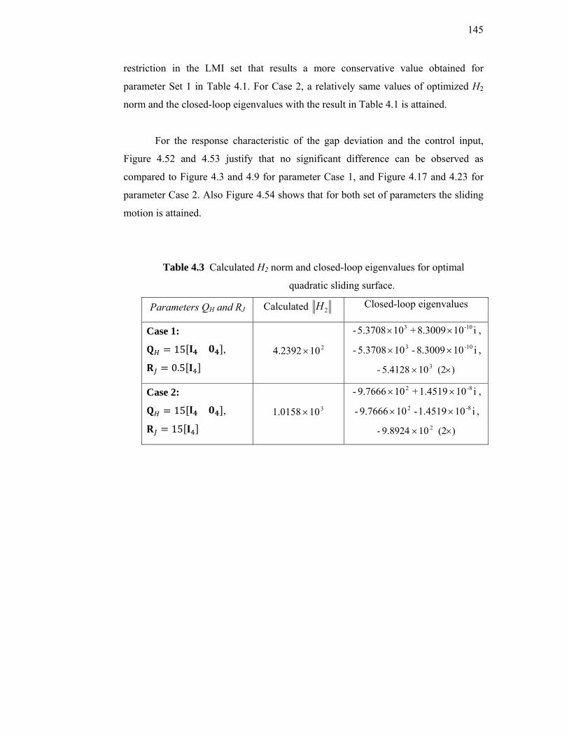
145

restriction in the LMI set that results a more conservative value obtained for

parameter Set 1 in Table 4.1. For Case 2, a relatively same values of optimized H2

norm and the closed-loop eigenvalues with the result in Table 4.1 is attained.

For the response characteristic of the gap deviation and the control input,

Figure 4.52 and 4.53 justify that no significant difference can be observed as

compared to Figure 4.3 and 4.9 for parameter Case 1, and Figure 4.17 and 4.23 for

parameter Case 2. Also Figure 4.54 shows that for both set of parameters the sliding

motion is attained.

Table 4.3 Calculated H2 norm and closed-loop eigenvalues for optimal

quadratic sliding surface.

Parameters QH and RJ Calculated 2H Closed-loop eigenvalues

Case 1:

15 ,

0.5

2104.2392 ×

i108.3009+ 105.3708- -103 ×× ,

i108.3009- 105.3708- -103 ×× ,

)(2 105.4128- 3 ××

Case 2:

15 ,

15

3101.0158 ×

i101.4519+ 109.7666- -82 ×× ,

i101.4519- 109.7666- -82 ×× ,

)(2 109.8924- 2 ××

146

Figure 4.52 Trajectories of X1 with optimal sliding surface

Figure 4.53 Control input with optimal sliding surface

147

Figure 4.54 Sliding surface σ1 with optimal sliding surface

4.3.3 Surface Parameterization with Robust Constraint of Pole-placement in

LMI Region

In this section the robust pole-placement in LMI region is imposed as the

only constraint in the LMI sets to calculate the sliding surface parameters. Table 4.4

tabulates the values of the c1 with the associated calculated closed-loop eigenvalues.

As can be noticed, the real value of eigenvalues is significantly smaller that the result

obtained by Set 1 and Table 4.3.

Figure 4.55 shows that for both c1 values, the gap deviation oscillates in

small magnitude and for c1 = 1000, the response has a longer settling time. The

reason is when c1 = 1000 is chosen, LMI region is set smaller and the resulted

eigenvalues are ‘pushed’ towards less negative real values that produces a longer

settling time. In term of control input, for c1 = 1000, the input current hits the

saturation level when the system is starting up as shown in Figure 4.56. Also with

148

this low value of c1, as illustrated by Figure 4.57, the sliding surface is reached at a

relatively longer time due to the saturated input.

Table 4.4 Closed-looped eigenvalues for sliding surface with robust pole-

placement constraint

Parameters c1 Closed-loop Eigenvalues

1000 346.7805- , 348.2496- ,

347.9276- , 347.4361- .

3500 101.1878- 3× , 101.1694- 3× ,

101.1805- 3× , 101.1758- 3× .

Figure 4.55 Trajectories of X1 with LMI constraint pole-placement sliding surface

149

Figure 4.56 Control input with LMI constraint pole-placement sliding surface

Figure 4.57 Sliding surface σ1 with LMI constraint pole-placement sliding surface

150

4.4 The Effect of Design Parameter, , on System Performance

To study the effect on the system performance when the parameter that

bounds the uncertainties is varied, the parameter setting Set 1 of MO-SMC used in

Section 4.3.1.1 is retained. For the following simulations, in addition to the value

10.7, two additional values are used as follows:

i. 2, (Not satisfying equation (3.12))

ii. )(tη = 50 (Conservatively satisfying equation (3.12))

The parameter 2 is chosen to represent the case where the condition imposed

by equation (3.12) is not satisfied which implies the nonlinear controller gain is too

small to remove the effect of uncertainties and disturbance that present in the system.

For 50, the value does satisfying the equation (3.12), however, the value is

set too large to bound the uncertainties. This means that the gain of the nonlinear

controller term is conservatively large which entails a lot of control effort is used to

overcome the uncertainties and disturbance. (Note: for the simulation result the

Greek symbol ρ is used to represent ).

Figure 4.58 shows that for 2 , the gap deviation has a longer settling

time and oscillates when reaching steady state. This agrees with the theoretical result

where the gain set is not adequate to eliminate the effect of the uncertainties and

disturbance. When 50 there is an overshoot in the response before reaching

zero steady state value. For the control input, when the system reach steady-state, the

input current for all the values are relatively the same, except for 50, the

input current reaches the saturation level at the system start-up (Figure 4.59). Figure

4.60 illustrate that for value of that is not satisfying the equation (3.12), the

system does not attain the sliding mode, but oscillates in the vicinity of sliding

surface.

151



152


4.5 The Effect of Design Parameters, and , on Chattering Elimination

The purpose of the following simulation is to investigate the effect of varying

the parameters and in eliminating the chattering in the control input. The

parameter determines the thickness of the boundary layer of the sliding surface

plays the major role in suppressing the chattering and the parameter only sets the

decay rate of the surface. However, since the parameter г determines the

convergence of the boundary layer, it has a very inconsiderable effect in eliminating

the input chatter and thus, 0.001 (constant) is used for this simulation. To

quantify the effect of chattering the so-called total power consumed index, Te shown

by equation (3.85) is used gauge chattering effect present in the control input since

high chattering effect implies large power consumption. Table 4.5 shows the chosen

values and the corresponding Te.

153

Table 4.5 and the power consumption index, Te.

0.5 0.5344

0.0005 0.5288

0.00001 0.7694

The tabulated Te values show that as the thickness of the boundary layer is

decreased, the Te value increases. This agree with the theoretical result in which the

thinner the boundary layer is, the higher the chattering effect in the input that results

in higher energy being consumed by the system. Figures 4.61 – 4.63 illustrate the

state X1, input current and sliding surface σ1, respectively. For 0.5, X1

oscillates within the boundary layer at steady state and the system never attains the

sliding mode but continuous input current is acquired. For thin boundary layer =

0.00001, X1 is regulated very effectively and the system enter the sliding motion at

the cost of high chattering effect which results in large power consumption. From

this simulation, = 0.0005 is the ‘optimum’ value for the trade-off between these

conflicting requirement.


154



155

4.6 The Effect of Bias Current, Ib, on System Performance

It is known that high bias current, Ib, in AMB system will improve the

damping of the system due to higher magnetic stiffness. In contrary, the main

disadvantage of this high current is additional power consumption is utilized. In this

section, the study on the performance of the system under variation of bias current is

carried out.

Table 4.6 shows the Te index for various bias current set for the simulation.

One can notice that as the bias current increases, so does the Te index which reflects

the increases in power consumption. However, for Ib = 0.8 A, it produces a higher Te

index due to the fact that, the system is difficult to be stabilized with this low bias

current. Figure 4.64 shows this effect where the gap deviation, X1, oscillates with

considerably large amplitude at steady-state. Figure 4.65 further illustrates that with

this Ib = 0.8, the rotor experience a whirling effect. Also, for operation under bias

current Ib = 0.8 and Ib = 0.9, the maximum gap deviation allowed by the actual

physical system is -4105.5 × m is violated and will cause the rotor to rub the stator.

For high bias current Ib = 1.8, the good damped system response is achieved at the

cost of high power consumption.

Table 4.6 Bias current, Ib and power consumption index, Te.

Ib [A]

0.8 0.5058

0.9 0.4766

1.0 0.5288

1.8 1.349

156

Figure 4.64 Trajectories of X1 (Varying Ib)

Figure 4.65 Rotor orbit for X1 vs. X3 (Varying Ib)

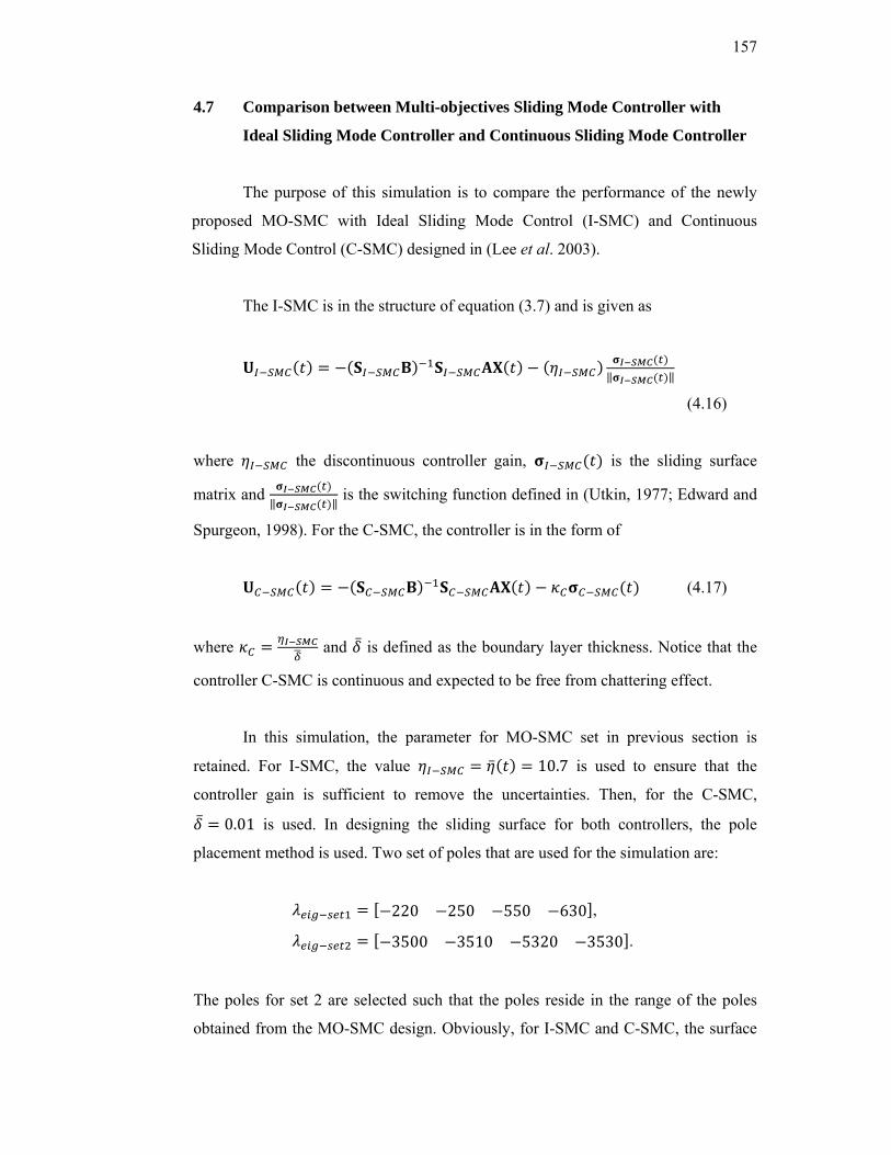
157

4.7 Comparison between Multi-objectives Sliding Mode Controller with

Ideal Sliding Mode Controller and Continuous Sliding Mode Controller

The purpose of this simulation is to compare the performance of the newly

proposed MO-SMC with Ideal Sliding Mode Control (I-SMC) and Continuous

Sliding Mode Control (C-SMC) designed in (Lee et al. 2003).

The I-SMC is in the structure of equation (3.7) and is given as

(4.16)

where the discontinuous controller gain, is the sliding surface

matrix and is the switching function defined in (Utkin, 1977; Edward and

Spurgeon, 1998). For the C-SMC, the controller is in the form of

(4.17)

where and is defined as the boundary layer thickness. Notice that the

controller C-SMC is continuous and expected to be free from chattering effect.

In this simulation, the parameter for MO-SMC set in previous section is

retained. For I-SMC, the value 10.7 is used to ensure that the

controller gain is sufficient to remove the uncertainties. Then, for the C-SMC,

0.01 is used. In designing the sliding surface for both controllers, the pole

placement method is used. Two set of poles that are used for the simulation are:

220 250 550 630 ,

3500 3510 5320 3530 .

The poles for set 2 are selected such that the poles reside in the range of the poles

obtained from the MO-SMC design. Obviously, for I-SMC and C-SMC, the surface

158

parameters, S, obtained from the procedure outlined in Section 3.3 cannot be adapted

due to the different structure of the equivalent control term. However, with the

selection of , the resulted sliding surfaces will closely reflect the region of

the closed-loop poles obtained from the MO-SMC.

Figure 4.66 shows the response of the system for the three types of

controllers. The poles set 1 are used for I-SMC and C-SMC in the simulation. In this

context, it can be seen that MO-SMC performs significantly better that I-SMC and

C-SMC where the settling time is shorter and less oscillation occur at steady state.

When the poles set 2 are used, the response of the system is shown in Figures 4.67-

4.70. The result shows that the response for all the controllers are relatively the same

except for I-SMC and C-SMC, a considerable overshoot occurs before the gap

deviation reach zero steady-state value. However, when looking at the control input

shown in Figures 4.71-4.74, it is obvious that the I-SMC contains undesirably high

chattering effect. Also, for C-SMC, although it is a continuous type controller, it can

be seen that input reaches its saturation level during most of the simulation time. This

is due to the fact that the C-SMC has to consume more power and hit the allowable

current limit to meet the desired system response. For MO-SMC, the continuous

input signal is achieved to obtain the desired response and less power consumption is

required as shown in Table 4.7. Figures 4.75-4.78 show that the under I-SMC, the

sliding surface contains high chattering effect and oscillates in the vicinity of sliding

surface. Analogously, the similar sliding surface for C-SMC also can be observed

due to the saturation of the control input. The figure justifies that the sliding surface

under MO-SMC has almost no oscillations and the sliding mode is attained.

Table 4.7 Maximum power consumption of AMB for MO-SMC,

I- SMC and C-SMC with the associated controller gains.

Controllers

I-SMC 0.7147

C-SMC 0.80

MO-SMC 0.5288

159

Figure 4.66 Trajectories of X1 of I-SMC, C-SMC and MO-SMC ( )


160



161


Figure 4.71 Control input of I-SMC, C-SMC and MO-SMC

162



163


Figure 4.75 Sliding surface σ1 of I-SMC, C-SMC and MO-SMC

164



165


4.8 Summary

The simulation work on the application of the newly proposed MO-SMC on

the AMB system under various conditions has been thoroughly studied in this

chapter. The performance of the controllers under various combinations of controller

parameters has been demonstrated which proves that the MO-SMC is invariant to the

uncertainties and disturbance that present in the system. Besides, the simulations

results also show the flexibility in the controller design where there are many

combinations and selections of controller parameters can be formed to achieve

satisfactory system response in eliminating uncertainties at low power consumption.

It is also shown that the controller has able to give excellent system

performance at a wide range of rotor rotational speed and various bias current which

specifically a new contribution in the area of control of AMB system. The

comparison between the MO-SMC, I-SMC and C-SMC demonstrates that the MO-

SMC has achieved better capability in giving desired good system response as to

166

compare to its counterparts. In addition, the design of MO-SMC is more well-

structured in which the controller parameters can be systematically determined

through solving the multi-constraint LMI set as opposed to the pole-placement

method where the selection of the poles heuristically to produce desirable response

may be time consuming. Concisely, the proposed MO-SMC with multi-objective

surface criteria achieves the design objective in controlling the AMB system to meet

the desired system performance and eliminating the effect of uncertainties and

disturbance present in the system under the continuous low-power control input.

197

CHAPTER 5

CONCLUSION AND SUGGESTIONS 5.1 Conclusion

This thesis is concerned with the design of a new nonlinear robust control

technique and its application into AMB system. The procedure mainly involves two

parts which are: 1) the modeling of the nonlinear AMB system and restructuring it

into a class of uncertain system that serve the basis for controller design, 2) the

development of the robust controller based on SMC theory in which the algorithm

include the design of the sliding surface and the continuous control law.

The formulation of the mathematical dynamic model that represents the AMB

system is outlined in which the major AMB nonlinearity effects which are the speed

dependant gyroscopic effect, nonlinear electromagnetic force and imbalance are

included in the model. Treating the coil currents as the system inputs, the rotor

dynamics are integrated with the electromagnetic dynamics to form the complete

nonlinear AMB model representing the more realistic AMB system. Since the

allowable operational range of the airgap, the rate of change of the airgap, the rotor

rotational speed and the maximum coil input currents are known, the upper and

lower bounds of the system nonlinearities and uncertainties is obtained and the

system can be rearranged to form a class of uncertain system by using deterministic

approach.

In order to perform the control on the AMB system, the sliding mode control

theory is adapted in which a new sliding surface design and a continuous control law,

168

or namely called MO-SMC are proposed. The new sliding surface has the advantages

of fulfilling multiple performance requirement of the closed-loop system in the

sliding motion. Each desired system performance that is essentially represented in

convex LMI set is then formulated to form complete LMI sets and the solution is

obtained by solving the sets using available LMI numerical solver. Specifically in

this work, the sliding surface desired characteristic is formed by formulating LQ

optimal surface and robust pole-clustering residing in a convex LMI region. For the

optimal characteristic, the design parameters are selected such that the H2 norm

objective function is minimized and desired system response is achieved while for

the robust pole clustering, an LMI region that ensures the poles reside in the LMI

area where the bounds form as the design parameters. The surface design is

developed in such a way that the algorithm can be easily amended to accommodate

other desired closed-loop performance such as minimization of mismatched

uncertainty effect in which the solution can be obtained systematically, as opposed to

heuristically selecting the surface parameters.

In the control law development, a new continuous robust SMC controller is

proposed. The controller combines the equivalent control and the exponentially

decaying boundary layer techniques in which by using the reaching condition, the

system states are guaranteed to reach the sliding surface in finite time, even with the

present of the system uncertainties and nonlinearities.

With the complete surface parameterization and the continuous control law

being applied on the nonlinear AMB dynamic model, the effectiveness of the control

performance has been demonstrated through extensive simulations. The robust

performances of the system under wide range of system conditions have been

achieved and this agrees with the theoretical finding. Many combinations of the

surface and control law parameters are also used to access the performance in which

the result shows that the developed algorithm does provide design flexibility.

In order to show the superiority of the newly proposed MO-SMC controller,

benchmarking with I-SMC and C-SMC shows that MO-SMC does provide superior

performance due to its chattering elimination feature and optimized stable closed-

loop performance.

169

Thus, the major contributions of this research can be concluded to be as

follows:

I. A new representation of the AMB system as a class of a nonlinear system

has been formulated and by using deterministic method, the model is

transformed into an uncertain system for controller design.

II. The design of a new sliding surface that can accommodate many

performance objectives in convex formulation. The solution can be

systematically obtained by using LMI technique which produces the

desired sliding surface parameter.

III. The design of a new continuous SMC control law that is able to eliminate

or attenuate the chattering while the reaching condition is guaranteed. The

complete control algorithm of the surface and control law form a new

complete SMC controller that is parameterized systematically and able to

provide robust performance with the present of system nonlinearities and

uncertainties.

IV. Validation of this new robust controller on nonlinear AMB system by

extensive computer simulation in which the evaluation of the performance

is accessed with various combinations of design parameters.

5.2 Recommendation of Future Works

Based on this work, the direction of the future research can be taken in two

ways concurrently which are developing a mathematical AMB model that also

include the second order nonlinearity effect and also the formulation of control law

that can ensure robust performance is achieved. The formulation of the complete

model that is close to the realistic AMB system model will provide the platform for

rigorous study of the dynamic of the system while development of robust controller

on such a model guarantees the satisfactory system response can be achieved under

actual physical condition and thus more directly applicable to real system.

Specifically to the scope of this work, the following suggestions for future works are

recommended:

170

i) Besides the inclusion of the second nonlinearity effects in the dynamic

model, AMB system with moving base is considered in the modeling

such that the model can cater broader range of application,

ii) The use and integration of adaptive technique with the MO-SMC to adjust

the bias current such that the optimal value can be achieved to minimize

steady state power loss,

iii) Application of the MO-SMC controller on the real AMB system such that

the actual performance can be verified experimentally, and

iv) With the availability of experimental set-up, identification method can be

proposed to obtain the uncertain bound which produces less conservative

controller gain.

171

LIST OF PUBLICATIONS

Husain, A.R., Ahmad, M.N. and Mohd Yatim, A.H. (2008). Application of H2 –

Based Sliding Mode Control of Active Magnetic Bearing System.

International Journal of Mechanical System Science and Engineering. 2(1):

pp. 1-8.

Husain, A.R., Ahmad, M.N. and Mohd Yatim, A.H. (2008). Asymptotic Stabilization

of Active Magnetic Bearing System using LMI-based Sliding Mode Control

of. International Journal of Mechanical System Science and Engineering.

2(1): pp. 9-16.

Husain, A.R., Ahmad, M.N. and Mohd Yatim, A.H. (2008). Chattering-free Sliding

Mode Control for an Active Magnetic Bearing System. International Journal

of Mechanical System Science and Engineering. 2(1): pp. 48-53.

Husain, A.R., Ahmad, M.N. and Mohd Yatim, A.H. (2007). Deterministic Models of

Active Magnetic Bearing System. International Journal of Computers. 2(8):

pp. 9-17.

Ahmad, M. N., Husain, A. R. and Mohd. Yatim, A. H. (2008). Sliding Mode Control

in Malaysia: A Brief Review on its Research Scope and Trend. in

Proceedings of 2008 Student Conference on Research and Development

(SCOReD 08), November. Johore Bahru, Malaysia.

Husain, A.R., Ahmad, M.N. and Mohd Yatim, A.H. (2007). Sliding Mode Control

with Linear Quadratic Hyperplane Design: An Application to Active

Magnetic Bearing System. in proceedings of 5th Student Conference on

Research Development (SCOReD 07), Dec. 11-12, Bangi, Selangor.

172

Husain, A.R., Ahmad, M.N. and Mohd Yatim, A.H. (2007). A New LMI-Based

Sliding Mode Control of An Active Magnetic Bearing System. International

Conference on Robotics, Vision, Info. & SignalProcessing. (ROVISP 07),

Nov. 28-30, Penang.

Husain, A.R., Ahmad, M.N. and Mohd Yatim, A.H. (2007). Sliding Mode Control of

An Active Magnetic Bearing System. National Intelligent System and

Information Technology Symposium (ISITS 07), Oct. 30-31, UPM, Serdang.

Husain, A.R., Ahmad, M.N. and Mohd Yatim, A.H. (2007). Sliding Mode Control of

an Active Magnetic Bearing System with Complex Valued Sliding Manifold.

International Conference on Control, Instrumentation & Mechatronics

(CIM’07), May 28-29, 2007, Johore Bahru, Malaysia.

Husain, A.R., Ahmad M.N. and Mohd Yatim A.H. (2007). Modeling of A Horizontal

Active Magnetic Bearing System with Uncertainties in Deterministic Form.

International Conference in Modelling & Simulation (AMS2007), March 27-

30, 2007, Phuket, Thailand.

Husain, A.R., Ahmad, M.N. and Mohd Yatim A.H. (2006). Modeling of A Nonlinear

Conical Active Magnetic Bearing System with Rotor Imbalance and Speed

Emf. International Conference in Man-Machines Systems (ICoMMS), Sept

15-16, Langkawi, Malaysia.

Husain, A.R., Ahmad, M.N. and Mohd Yatim, A.H. (2006). Elimination of

Mismatched Imbalance Vibration of Active Magnetic Bearing System Using

Full Order Sliding Mode Controller. Regional Postgraduate Conference in

Engineering and Science (RPCES), July 26-27, 2006, SPS UTM, Malaysia.

173

REFERENCES

Ahmad, M. N. (2003). Modelling and Control of Direct Drive Robot Manipulators.

PhD. Thesis. Universiti Teknologi Malaysia, Johore, Malaysia.

Ahmad, M. N. and Osman, J. H. S. (2003). Application of proportional-integral

sliding mode tracking controller to robot manipulators. In Proceedings of IEEE

Conference on Control Applications. June 23-25. : 87-92.

Allaire, P. E. , Mikula, A., Banejee, B. B., Lewis, D. W. and Imlach, J. (1989).

Design and test of a magnetic thrust bearing. Journal of Franklin Institute.

326(6): 831-847.

Anderson, B. D. O. and Moore, B. (1990). Optimal Control – Linear Quadratic

Method. Prentice Hall. New Jersey, USA.

Antila, M., Lantto, E. and Arkkio, A. (1998). Determination of Forces and

Linearized Parameters of Radial Active Magnetic Bearings by Finite Element

Technique. IEEE Transactions on Magnetics. May. 34(3): 684-694.

Arzelier, D., Bernussou, J. and Garcia, G. (1993). Pole Assignment of Linear

Uncertain System in a Sector via Lyapunov-Type Approach. IEEE

Transactions on Automatic Control. July. 38(7): 1128-1132.

Bartoszewics, A. and Patton, R. J. (2007). Sliding Mode Control-Editorial.

International Journal of Adaptive Control and Signal Processing. August. 21:

635-637.

Betschon, F and Knospe, C. R. (2001). Reducing Magnetic Bearing Current via Gain

Scheduled Adaptive Control. IEEE/ASME Transactions on Mechatronics.

December. 6(4): 437-443.

Bi, C., Wu, D., Jiang, Q. and Liu Z. (2005). Automatic Learning Control for

Unbalance Compensation in Active Magnetic Bearings. IEEE Transactions on

Magnetics. July. 41(7) : 2270-2280.

174

Bleuler, H. (1992). Survey of magnetic levitation and magnetic bearing types. JSME

International Journal, Series 3: Vibration, Control Engineering, Engineering

for Industry. September. 35(3): 335-342.

Bleuler, H., Vischer, D., Schweitzer, G., Traxler, A. and Zlatnik, D. (1994a).New

concepts for cost-effective magnetic bearing control. Automatica. May. 30(5):

871-876.

Bleuler, H., Gahler, C., Herzog, R., Larsonneur R., Mizuno, T., Siegwart, R. and

Woo, S. J. (1994b). Application of Digital Signal Processors for Industrial

Magnetic Bearings. IEEE Transaction on ControlSystems Technology.

December. 2(4): 280-289.

Bosgra, O. H., Kwakernaak, H. and Meinsma, G. (2007). Design Method for Control

System. Lecture Note for DISC. Holland.

Boyd, S. Ghaoui, L. E., Feron, E., and Balakrishnan, V. (1994). Linear matrix

inequality in systems and control theory. SIAM. Philadelphia, USA.

Buckholtz, K. R. (2002). Approach Angle-Based Switching Function for Sliding

Mode Control Design. In Proceedings of the American Control Conference.

Anchorage AK, USA. May 8-10: 2368-2373.

Buckner, G. D. (2002). Intelligent Bounds on Modeling Uncertainty: Applications to

Sliding Mode Control. IEEE Transactions on System, Man, and Cybernatics. –

Part C: Application and Review. May. 32(2): 113-124.

Cao, W. J., and Xu, J. X. (2004) Nonlinear Integral-Type Sliding Surface for Both

Matched and Unmatched Uncertain Systems. IEEE Transactions on Automatic

Control. 49(8): 1355- 1360.

Charara, A., Miras, J. D., and Caron, B. (1996). Nonlinear Control of a Magnetic

Levitation System Without Premagnetization. IEEE Transaction on Control

System Technology. September. 4(5): 513-523.

Chen, B. (2000). Robust and H-Infinity Control. Springer. London, UK.

Chen, M. S., Hwang, Y. R., and Tomizuka M. (2002). A State-Dependent Boundary

Layer Design for Sliding Mode Control. IEEE Transaction on Automatic

Control. October. 47(10): 1677-1681.

Chen, M. and Knospe, C. R. (2005). Feedback Linearization of Active Magnetic

Bearings: Current-Mode Implementation. IEEE/ASME Transaction on

Mechatronics. December. 10(6): 632-639.

175

Chen, H. M., Renn, J. C. and Su, J. P. (2005a). Sliding Mode Control with Varying

Boundary Layers for an Electro-Hydraulic Position Servo System.

International Journal of Advance Manufacturing System. January. 26: 117-123.

Chen, S. L., Chen, S. H. and Yan, S. T. (2005b). Experimental Validation of a

Current-Controlled Three-pole Magnetic Rotor-Bearing System. IEEE

Transactions on Magnetics. January. 41(1) : 99-112.

Chilali, M., and Gahinet, P. (1996), H∞ Design with Pole Placement Constraint: An

LMI Approach. IEEE Transaction on Automatic Control. March. 41(3): 358-

367.

Chilali, M., Gahinet, P., and Apkarian, P. (1999). Robust Pole Placement in LMI

Regions. IEEE Transaction on Automatic Control. December. 44(12): 2257-

2270.

Choi, C. Y. (2002). Investigation on the Whirling Motion of Full Annular Rotor Rub.

Journal of Sound and Vibration. 258(1): 191-198.

Choi, H. H. (2007). An LMI-Based Switching Surface Design for Integral Sliding

Mode Control of Mismatched Uncertain Systems. IEEE Transaction on

Automatic Control. 52(4): 736-742.

Choi, H. H. (1998). An Explicit Formula of Linear Sliding Surfaces for a Class of

Uncertain Dynamic systems with Mismatched Uncertainties. Automatica.

34(8): 1015-1020.

Choi, H. H. (1997). A New Method for Variable Structure Control System Design: A

Linear Matrix Inequality Approach. Automatica. 33(11): 2089-2092.

Cole, M. O. T., Keogh, P. S., Sahinkaya, M. N., and Burrows, C. R. (2004). Towards

fault-tolerant active control of rotor-magnetic bearing systems. Control

Engineering Practice. 12: 491-501

DeCarlo, R. A., Zak, S. H., and Mathews, P. (1988). Variable Structure Control of

Nonlinear Multivariable Systems: A Tutorial. Proceedings of IEEE. March

1988. 76(3): 212-232.

DeQueiroz, M.S., Dawson, D.M. and Suri, A. (1998). Nonlinear Control of a large-

gap 2-DOF magnetic bearing system based on a coupled force model. IEE

Proceeding on Control Theory and Application. May. 145(3): 269-276.

DeQueiroz, M.S. and Dawson, D.M. (1996a). Nonlinear Control of Active Magnetic

Bearings: A Backstepping Approach. IEEE Transaction on Control System

Technology. September. 4(5): 545-552.

176

DeQueiroz, M.S. and Dawson, D.M. (1996b). A Backstepping-type Controller for a

6-DOF Active Magnetic Bearing System. In Proceedings of IEEE

International Conference on Control Application. December, Kobe, Japan.

3370-3375.

Diong, B. M. and Medanic, J. V. (1997). Simplex-type variable structure controllers

for system with non-matched disturbance and uncertainties. International

Journal of Control. 68(3): 625-656.

Dorf, R. C. and Bishop, R. H. (1995). Modern Control System. Addison Wesley.

Massachusetts, USA.

Dullerud, G. E. and Pagadini, F. G. (2005). A Course in Robust Control Theory: A

Convex Approach. Text in Applied Mathematics. Springer. UK.

Earnshaw, S. (1842). On the nature of the Molecular Forces Which Regulate the

Constitution of the Lumiferous Ether. Transaction of Cambridge Philosophical

Society 7: 97-112.

Edwards, C. (2004) A practical method for the design of sliding mode controllers

using linear matrix inequality. Automatica. 40: 1761-1769

Edwards, C., and Spurgeon, S. (1998). Sliding Mode Control: Theory and

Applications. Taylor and Francis. London, UK.

El-Ghezawi, O. M. F., Zinober, A. S. I. and Billings, S. A. (1983). Analysis and

Design of Variable Structure System using Geometric Approach. International

Journal of Control. 38: 657-671.

Fabien, B. C. (1996). Observer-based feedback linearizing control of an

electromagnetic suspension. ASME Journal of Dynamic Systems, Measurement

and Control. 118(3): 615-619.

Farrera, A. (2005). A variable structure convex programming based control approach

for a class of uncertain linear systems. System and Control Letters. 54: 529-538

Fittro, R. L. and Knospe, C. R. (2002). Rotor Compliance Minimization Via µ-

Control of Active Magnetic Bearings. IEEE Transaction on Control System

Technology. March. 10(2): 238-249.

Font, S., Duc, G. and Carrere, F. (1994). H∞ Control of Magnetic Bearing. In

Proceedings of IEEE Conference on Control Applications. Aug 24-26.

Glasgow, UK. 581-585.

177

Fujita, M., Matsumura, F. and Uchida, K. (1990). Experiment on the H∞ disturbance

attenuation control of a Magnetic Suspension System. In Proceedings of the

IEEE 28th Conference on Decision and Control, Hawaii, USA. 5: 2773-2778.

Fujita, M., Hatake, K. and Matsumura, F. (1993). Loop Shaping Based Robust

Control of a Magnetic Bearing. IEEE Control System Magazine. August. 13(4):

57-65.

Fujita, M., Namerikawa, T., Matsumura, F. and Uchida, K.(1995). μ-Synthesis of an

Electromagnetic Suspension System. IEEE Transaction on Automatic Control.

Marc. 40(3): 530-536.

Fujita, M., Tokumasu, T., Yamada, T., Hirose, T., Tanaka, Y., Kumagai, N. and

Uchida, S. (1998). 3-Dimensional Electromagnetic Analysis and Design of an

Eddy-Current Rail Brake System. IEEE Trans. on Magnetics. September.

34(5): 3548-3551.

Gahinet, P. and Apkarian. P. (1994). A Linear Matrix inequality Approach for H∞

Control. International Journal of Robust and Nonlinear Control. 4(5): 421-

448.

Gahinet, P., Nemirovski, A., Laub, A., and Chilali, M. (1995). LMI control toolbox,

user guide. Natick, MA: Mathworks, Inc.

Gao W. B., and Hung J. C. (1993). Variable structure control of nonlinear systems:

A New approach. IEEE Transactions on Industrial Electronics. February. 1993

40: 45-55.

Gibson, N. S., Choi, H. and Buckner, G. D. (2003). H Control of Active Magnetic

Bearings Using Artificial Neural Network Identification of Uncertainty. 2003.

In IEEE Proceedings of International Conference on System, Man and

Cybernetics. October 5-8. Washington DC. USA. : 1449-1456.

Grochmal, R., and Lynch, A. F. (2007). Experimental comparison of nonlinear

tracking controllers for active magnetic bearings. Control Engineering

Practice. 15: 95-107.

Gutman, S. and Jury, E. I. (1981). A General Theory for Matrix Root-Clustering in

Subregion of the Complex Plane. IEEE Transaction on Automatic Control.

August. AC-26(4): 853-863.

Hartavi, A. E., Tuncay, R. N. and Gurleyen, F. (2001). The Design, Simulation and

Experimental Study of Active Magnetic Bearing . Proc. IEEE, 2001.

178

Hassan I. M. M. (2002). Modern Robust Control of Magnetic Bearing System with

Imbalanced Rotor. Ph. D. Thesis, Assiut University, Egypt.

Hassan, I. M. M. and Mohamed, A. F. (2001). Variable Structure Control of

Magnetic Levitation System. in Proceedings of American Control Conference.

June 25-27. Arlington, Virginia, USA: 3725-3730.

Henrion, D. (2007). Course Note on LMI Optimization with Application in Control.

Czech Technical University in Prague.

Herrmann, G., Turner, M. C. and Postlethwaite, I. (2007). Linear Matrix Inequality

in Control. - Lecture Notes in Control and Information Sciences, Mathematical

Methods for Robust and Nonlinear Control. Book Chapter, Springer. Berlin.

Hermann G., Spurgeon, S. and Edwards, C. (2001). A Robust Sliding Mode Output

Tracking Control for a Class of relative degree zero and non-minimum phase

plants: A Chemical Process Application. International Journal of Control.

74(12): 1194-1209.

Herzog, R., Buhler, P., Gahler, C. and Larsonneur R. (1996). Unbalance

Compensation Using Generalized Notch Filters in the Multivariable Feedback

of Magnetic Bearings. IEEE Transaction on Control System Technology.

September. 4(5): 580-586.

Hong, S. K. and Langari, R. (2000). Robust Fuzzy Control of Magnetic Bearing

System subjected to Harmonic Disturbance. IEEE Transaction on Control

System Technology. March. 8(2): 366-371.

Hong, S. K. and Nam, Y. (2003). Stable Fuzzy Control System Design with Pole-

Placement Constraint: an LMI Approach. Computer in Industry. 51: 1-11.

Hsu, C. T. and Chen, S. L. (2003). Nonlinear control of a 3-pole active magnetic

bearing system. Automatica. 39:291-298.

Hsu, C. T. and Chen, S. L. (2002). Exact Linearization of a Voltage-Controlled 3-

Pole Active Magnetic Bearing System. IEEE Transaction on Control System

Technology. July. 10(4): 618-625.

Hu, T., Lin, Z., and Allaire, P. E. (2004). Reducing Power Loss in Magnetic

Bearings by Optimizing Current Allocation. IEEE Transaction on Magnetics.

40(3): 1625-1635

Huang, J. Y., and Way, H. K. (2001a). Placing all closed poles of missile attitude

control systems in the sliding mode via the root locus technique. ISA

Transactions. 40: 333-340

179

Huang, J. Y., and Way, H. K. (2001b). Design of sliding surfaces in variable

structure control via a direct pole assignment scheme. International Journal of

Systems Science. 40(8): 963-969.

Huang, S. J., and Lin, L. C. (2003). Fuzzy Modelling and Control for Conical

Magnetic Bearings Using Linear Matrix Inequality. Journal of Intelligent and

Robotic Systems. August. 37: 209-232.

Huang, S. J., and Lin, L. C. (2004). Fuzzy Dynamic Output Feedback Control with

Adaptive Rotor Imbalance Compensation for Magnetic Bearing Systems. IEEE

Transaction on System, Man, and Cybernatics. – Part B: Cybernatics. August.

34(4): 1854-1864.

Huang, S. J., and Lin, L. C. (2005). Stable Fuzzy Control with Adaptive Rotor

Imbalance Compensation for Nonlinear Magnetic Bearing Systems. Journal of

the Chinese Institute of Engineers. 28(4): 589-603.

Hung, J. H. (1995). Magnetic Bearing Control Using Fuzzy Logic. IEEE Transaction

on Industry Application. November/December. 31(6): 1492-1497.

Hung, J. H., Gao, W., and Hung, J. C. (1993). Variable Structure Control: A Survey.

IEEE Transaction on Industrial Electronics. February. 1993. 40(1): 2-22.

Hung, J. Y., Albritton, N. G. and Xia, F. (2003). Nonlinear Control of Magnetic

Bearing System. Mechatronics. 13: 621-637.

Iwasaki, T., Skelton. R. E. and Geromel, C. J. (1994). Linear Quadratic Suboptimal

Control with Static Output Feedback. Systems and Control Letters. 23(6): 421-

430.

Jafarov, E. M. (2005). Robust Sliding Mode Controllers Design Techniques for

Stabilization of Multivariable Time-delay System with Parameter Perturbation

and External Disturbances. International Journal of System Science. June.

7(10): 433-444.

Jafarov, E. M., Parlakci, M. N. A and Istefanopolos, Y. (2005). A new Variable

Structure PID-Controller Design for Robot Manipulators. IEEE Transaction on

Control System Technology. Jan. 13(1): 122-130.

Jang M.-J, Chen C.-L. and Tsao Y.-M. (2005). Sliding Mode Control for active

magnetic bearing system with flexible rotor. Journal of Franklin Institute. 342:

401-419.

180

Joo and Seo. (1997). Design and Analysis of the Nonlinear Feedback Linearizing

Control for an Electromagnetic Suspension System. IEEE Transaction on

Control System Technology. Jan. 5(1): 135-144.

Kanebako, H. and Okada, Y. (2003). New Design of Hybrid-Type Self-Bearing

Motor for Small, High-Speed Spindle. IEEE/ASME Transaction on

Mechatronics. March. 8(1): 111-119.

Kasarda, M. E. F. (2000). An Overview of Active Magnetic Bearing System

Technology and Applications. The Shock and Vibration. March. 32(2): 91-99.

Kim, K. J., Park, J. B. and Choi, Y. H. (2006). Chattering Free Sliding Mode

Control. In SICE-ICASE International Joint Conference. Oct. 18-21. Busan,

Korea.

Kim, S. K. and Jabbari, F. (2000). Using Scales in the Multiobjective Approach.

IEEE Transaction on Automatic Control. May. 45(5): 973-977.

Kim, S. K., and Park, Y. (2004) Sliding Mode Design via Quadratic Performance

Optimization with Pole-Clustering Constraint. Siam Journal on Control

Optimization. 43(2): 670-684.

Kim, S. K., Park. Y. and Oh, S. W. (2000). Designing Robust Sliding Hyperplane for

Parametric Uncertain System: A Riccati Approach. Automatica. 36: 1041-

1048.

Knospe C. R. (2007). Active magnetic bearings for machining applications. Control

Engineering Practice. 15: 307-313.

Knospe C. R. and Collins E. G. (1996). Introduction to Special Issue on Magnetic

Bearing Control. IEEE Trans. on Control System Technology. Sept. 1996. 4(5):

481-483.

Laghrouche S., Plestan F., and Glumineau A. (2007). Higher order sliding mode

based on integral sliding mode. Automatica. 43: 531-537.

Lee, C. W. and Jeong, H. S. (1996). Dynamic Modeling and Optimal Control of

Cone Shaped Active Magnetic Bearing Systems. Control Engineering

Practice. 4(10): 1393-1403.

Lee, H., and Utkin, V. (2007). Chattering suppression methods in sliding mode

control systems. Annual Review in Control. 31: 179-188.

Lee J.-H., Allaire P. E., Tao G., Decker J. A. and Zhang X. (2003). Experimental

Study of Sliding Mode Control for a Benchmark Magnetic Bearing System and

181

Artificial Heart Pump Suspension. IEEE Transaction on Control System

Technology. Jan. 11(1): 128-138.

Lewis, A. S., Sinha, A., and Wang, K. W. (2001). Sliding Mode Output Feedback

Control of a Flexible Rotor Supported by Magnetic Bearings. International

Journal of Rotating Machinery. 7(2): 117-129.

Lewis, F. L., Abdallah C. T. and Dawson, D. M. (1993). Control of Robot

Manipulators. New York: Macmillan.

Levine, J., Lottin, J., and Ponsart, J. C. (1996). A Nonlinear Approach to the Control

of Magnetic Bearings. IEEE Transaction on Control System Technology.

September. 4(5): 524-544.

Li, G., Lin, Z., Allaire, P. E. and Luo J. (2006). Modeling of High Speed Rotor Test

Rig with Active Magnetic Bearings. ASME Journal of Vibration and Acoustics.

June. 128: 269-281.

Li, L. (1999). Linearizing magnetic bearing actuators by constant current sum,

constant voltage sum, and constant flux sum. IEEE Transaction on Magnetic.

.35(1): 528-535.

Li, L. and Mao, J. (1999). Feedback linearization of magnetic bearing actuators for a

uniform upper bound of force slew rate. IEE Proceedings of the Electric Power

Applications. 146(4): 378-382.

Liang, T. and Yiqing, C. (2007) Model Development and Adaptive Imbalance

Vibration Control of Magnetic Suspended System. Chinese Journal of

Aeronautics. 20: 434-442.

Liang Y. W., and Xu S. D. and Chu, T. C. (2007). Robust Control of the Robot

Manipulator via an Improved Sliding Mode Scheme. In Proceedings of IEEE

International Conference on Mechatronics and Automation. August 5-8.

Harbin, China: 1593-1598.

Lin, C. H. and Gau, T. B. (1997). Feedback Linearization and Fuzzy Control for

Conical Magnetic Bearings. IEEE Transaction on Control System Technology.

July. 5(4): 417-426.

Lin, C. T. and Jou, C. P. (2000) GA-Based Fuzzy Reinforcement Learning for

Control of Magnetic Bearing System. IEEE Transactions of System, Man and

Cybernatics- Part B: Cybernatics. April. 32(2): 276-289.

182

Lindlau J. D. and Knospe C. R. (2002). Feedback Linearization of an Active

Magnetic Bearing With Voltage Control. IEEE Transaction on Control System

Technology January. 10(1): 21-31.

Liu Z.-H. , Nonami K. and Ariga Y. (2002). Adaptive Unbalanced Vibration Control

of Magnetic Bearing Systems with Rotational Synchronizing and

Asynchronizing Harmonic Disturbance. JSME International Journal. Series C,

45(1): 142-149.

Lofberg, J. (2004). YALMIP : A Toolbox for Modeling and Optimization in

MATLAB. In Proceedings of the CACSD International Conference. Taiwan.

Losch F., Gahler C. and Herzog R. (1999). Low Order μ-Synthesis Controller Design

for a Large Boiler Feed Pump Equipped with Active Magnetic Bearings. In

Proceedings of IEEE International Conference on Control Application. August

22-27, 1999: 564-569

Lu, B., and Wu, F. (2004). Switching LPV control designs using multiple parameter-

dependent Lyapunov functions. Automatica. 40:1973-1980.

Lu, B., Choi, H., Buckner, D. and Tammi, K. (2008). Linear parameter-varying

techniques for control of a magnetic bearing system. Control Engineering

Practice. 16(10): 1161-1172.

Lum K.-Y., Coppola V. T. and Bernstein D. S. (1996). Adaptive Autobalancing

Control for an Active Magnetic Bearing Supporting a Rotor with Unknown

Mass Imbalance. IEEE Trans. on Contr. Syst. Tech. Sept. 1996. 4(5): 587-597.

Maslen, E., Sortore, C. K., Gillies, G. T., Williams, R. D., Fedigan, S. J. and

Aimone, R. J. (1999). Fault Tolerence Magnetic Bearings. ASME Journal of

Engineering for Gas Turbines and Power. 121(3): 504-508.

Mackenroth, U. (2004). Robust Control System: Theory and Case Study. Springer-

Verlag. New York, USA.

Matsumura, F. and Yoshimoto, T. (1986). System modeling and control design of a

horizontal shaft magnetic bearing system. IEEE Transaction on Magnetics.

May. MAG-22(3): 196-203.

Matsumura, F., Fujita, M. and Oida, C. (1987). Theory and Experiment of Magnetic

Bearing Combining Radial Control and Thrust Control. IEEE Transaction on

Magnetics. September. MAG-23(5): 2581-2583.

183

Matsumura, F., Fujita, M. and Okawa K.(1990). Modeling and Control of Magnetic

Bearing Systems Achieving a Rotation Around the Axis of Inertia. 2nd

International Symposium on Magnetic Bearing. July. Tokyo, Japan: 273-280.

Matsumura, F., Namerikawa, T., Hagiwara, K. and Fujita, M. (1996). Application of

Gain Scheduled H∞ Robust Controller to a Magnetic Bearing. IEEE

Transaction. on Control System Technology. September. 4(5): 484-493.

Matsumura, F., Namerikawa, T. and Murata, N. (1999). Wide Area Stabilization of a

Bearing Using Exact Linearization. Electrical Engineering in Japan. 128(2):

53-62.

Mohamed, A.M. and Emad, F.P. (1992). Conical Magnetic Bearings with Radial and

Thrust Control. IEEE Transaction on Automatic Control. Dec. 37(12): 1859-

1868.

Mohamed, A. M. and Emad, F. P. (1993). Comparison Between Current and Flux

Control in Magnetic Bearing Systems. In Proceedings of the American

Control. Conference, June 1993. 2356-2362.

Mohamed, A. M., Matsumura, F., Namerikawa, T., Lee J. H. (1997a). Q-

parameterization Control of Vibration in a Variable Speed Magnetic Bearing.

Proceeding of IEEE International Conference on Control Application,

October: 540-546.

Mohamed, A. M., Matsumura, F., Namerikawa, T., Lee J. H. (1997b) .Modeling and

Robust Control of Self-sensing Magnetic Bearing with Unbalance

Compensation. Proceeding of IEEE International Conference on Control

Application, October : 586-594.

Mohamed, A. M., Hassan, I. M., Hashem, A. M. K. (1999). Elimination of

Imbalance Vibrations in Magnetic bearing System Using Discrete-Time Gain-

Scheduled Q-Parameterization Controllers. Proceeding of IEEE International

Conference on Control Application, August. 737-742

Montee, N., De Queiroz M. S., Fang, Y. and Dawson D. M. (2002). Active Magnetic

Bearing Control with Zero Steady-State Power Loss. Proceedings of the

American Control Conference. May 8-10. Anchorage, AK, USA : 827-832.

Mukhopadhyay, S. C., Ohji, T., Iwahara, M. and Yamada, S. (2000). Modeling and

Control of a New Horizontal-Shaft Hybrid-Type Magnetic Bearing. IEEE

Transaction on Industrial Electronics. February. 40(1): 2-22.

184

Mukhopadhyay, S. C., Ohji, T., Iwahara, M., Yamada, S. and Matsumura, F. (1997).

Disturbance Attenuation and H∞ Control of Repulsive Type Magnetic Bearing.

IEEE Transaction on Magnetics. September. 33(5): 4233-4235.

Namerikawa, T. and Fujita, M. (2004). H∞ DIA Control of Magnetic Suspension

System. Proceedings of IEEE International Conference on Control

Application. Sept. 2-4. Taiwan: 1697-1702.

Namerikawa, T. and Shinozuka, W. (2004). H∞ Control of Magnetic Bearing System

Considering Initial State Uncertainties. IEEE International Workshop on

Advance Motion Control-AMC . Kawasaki, Japan: 275-280.

Namerikawa, T. and Fujita, M. (1999). Uncertain Model and μ-Synthesis of a

Magnetic Bearing. In Proceedings of IEEE International Conference on

Control Application. August 22-27. Hawaii, USA: 558-563.

Nesterov, Y. and Nemirovski, A. (1994). Interior Point Polynomial Methods in

Convex Programming: Theory and Applications. SIAM. Philadelphia, USA.

Nonami, K. and Ito, T. (1996). μ-Synthesis of Flexible Rotor-Magnetic Bearing

Systems. IEEE Transaction on Control System Technology. September. 4(5):

503-512.

Ogata, K. (2001). Modern Control Engineering-4th Edition. Prentice Hall. New

Jersey, USA.

Okada, Y. and Nonami, K. (2002). Research Trend on Magnetic Bearings. JSME

International Journal. Series C, 46(2): 341-343.

Osman, J. H. S. (1991). Decentralized and Hierarchical Control of Robot

Manipulator. Ph.D. Thesis, City University, London, UK.

Osman, J. H. S. and Roberts, P.D. (1995). Two-level Control Strategy for Robot

Manipulator. International Journal of Control. June. 61(6): 1201-1222.

Polajzer, B., Ritonja, J., Stumberger, G., Dolinar, D. and Lecointe, J. P. (2006).

Decentralized PI/PD Position Control for Active Magnetic Bearings.

Electrical Engineering. 89: 53-59.

Rundell, A. E., Drakunov, S. V. and DeCarlo, R. A. (1996). A Sliding Mode

Observer and Controller for Stabilization of Rotational Motion of Vertical

Shaft Magnetic Bearing. IEEE Transaction on Control System Technology.

September. 1996. 4(5): 598-608.

Saberi, A., Sannuti, P. and Chen. B. (1995). H2 Optimal Control. Prentice Hall.

London, UK.

185

Sahinkaya, M. N, Hartavi, A. E. (2007). Variable Bias Current in Magnetic Bearings

for Energy Optimization. IEEE Transaction on Magnetics. March. 43(3):

1052-1060.

Sahinkaya, M. N, Adulrub A. –H. G. and Keogh P. S. (2004). On the Modelling of

Flexible Rotor Magnetic Bearing Systems When in Contact with Retainer

Bearings. Proceedings of Ninth International Symposium on Magnetic

Bearings. August, 3-6. Kentucky, USA. 1-6.

Sam, Y. M., Osman, J. H. S. And Ghani, M. R. A. (2004). A Class of Proportional-

Integral Sliding Mode Control with Application to Active Suspension System.

Systems and Control Letters. 51:217-223.

Scherer C. and Weiland, S. (2004). Linear Matrix Inequalities in Control. Lecture

Notes in DISC Course. Holland.

Scherer C., Gahinet, P., and Chilali, M. (1997). Multiobjective Output-Feedback

Control via LMI Optimization. IEEE Transaction on Automatic Control. July.

42(7): 896-911.

Schroder, P, Green, B., Grum, N. and Flemming, P. J. (2001). On-line evolution of

robust control system: an active magnetic bearing application. Control

Engineering Practice. 9: 37-49.

Sellami, A., Arzelier D, M’hiri, R. and Zrida, J. (2007). A Sliding Mode Control

Approach for System Subjected to a Norm-bounded uncertainties.

International Journal of Robust and Nonlinear Control. 17:327-346.

Shafai, B., Beale S., LaRocca, P. and Cusson, E. (1994). Magnetic Bearing Control

System and Adaptive Forced Balancing. IEEE Control Systems Magazine.

April. 14(2): 4-13.

Shen, J. X., Tseng, K. J., Vilathagamuwa, D. M. and Chan W. K. (2000). A Novel

Compact PMSM with Magnetic Bearing for Artificial Heart Application. IEEE

Transaction on Industrial Applications. July/August. 36(4) :1061-1068.

Shi, J., Zmood, R. and Qin, L. (2004). Synchronous disturbance attenuation in

magnetic bearing using adaptive compensation signals. Control Engineering

Practice. 12: 283-290.

Sivrioglu, S. (2007). Adaptive backstepping for switching control active magnetic

bearing system with vibrating base. IET Proceedings on Control Theory

Application. 1(4): 1054-1059.

186

Sivrioglu, S. and Nonami, K. (2003). Adaptive Backstepping Control Design for

Flywheel Zero-Bias AMB. In Proceedings of IEEE Conference on Control

Application. June 23-25. Istanbul, Turkey: 1106-1111.

Sivrioglu, S. and Nonami, K. (1998). Sliding Mode Control with Time-Varying

Hyperplane for AMB Systems. IEEE/ASME Transaction on Mechatronics.

March. 3(1): 51-59.

Skogestad, S. and Postlethwaite, I. (2005). Multivariable Feedback Control: Analysis

and Design. Wiley. England.

Slotine, E. J. J. and Li, W. (1991). Applied Nonlinear Control. Prentice Hall. New

Jersey, USA.

Smith, R. D. and Weldon, W. F. (1995). Nonlinear Control of a Rigid Magnetic

Bearing System: Modeling and Simulation with Full State Feedback. IEEE

Transactions on Magnetics. March. 31(2): 973-980.

Stepanenko, Y., Cao, Y. and Su, C. Y. (1998). Variable Structure Control of Robotic

Manipulators with PID Sliding Surface. International Journal of Robust and

Nonlinear Control. 8: 79-90.

Sturm, J. F. (1999). Using SeDuMi 1.02, a MATLAB toolbox for optimization over

symmetric cones. Optimization Methods and Software- Special issue on

Interior Point Methods : 625-653.

Takahashi, R. H. C. and Peres, P. L. D. (1999). H2 Guaranteed Cost-Switching

Surface Design for Sliding Modes with Nonmatching Disturbances. IEEE

Transactions on Automatic Control. 44(11): 2214-2218.

Takahashi, R. H. C. and Peres, P. L. D. (1998). H∞ Design of Switching Surface for

Sliding Modes Control with Nonmatching Disturbances. IEE Proceedings on

Control of Theoretical Applications. 145: 435-441.

Tian, H. (1999). Robust Control of Spindle-Magnetic Bearing System Using Sliding

Mode Control and Variable Structure System Disturbance Observer. Journal of

Vibration and Control. 5: 277-298.

Tsiotras, P. and Wilson, B. (2003). Zero- and Low-Bias Control Designs for Active

Magnetic Bearings. IEEE Transaction on Control System Technology. Nov.

11(6): 889-904.

Tsiotras, P. and Arcak, M. (2005). Low-Bias Control of AMB Subject to Voltage

Saturation: State-Feedback and Observer Designs. IEEE Transaction on

Control System Technology. Marc. 13(2): 262-273.

187

Trumper, D. L., Olson, S. M. and Subrahmanyan, P. K. (1997). Linearizing Control

of Magnetic Suspension Systems. IEEE Transaction on Control System

Technology. July. 5(4): 427-438.

Tsai, N. C., Kuo, C. H., and Lee, R. M. (2007). Regulation on radial position

deviation for vertical AMB systems. Mechanical Systems and Signal

Processing. 21: 2777-2793.

Utkin, V. and Shi, J. (1996). Integral Sliding Mode in System Operating Under

Uncertainty Condition. In Proceedings of the IEEE Conference on Decision

and Control. December 11-13, Kobe, Japan; 4591-4596.

Utkin, V. (1992). Sliding Mode Control in Optimization. Springer. Berlin.

Utkin, V. (1977). Variable Structure Systems with Sliding Mode. IEEE Transactions

on Automatic Control. 22(2): 212-222.

VanAntwerp, J. G., and Braatz, R. D. (2000). A Tutorial on linear and bilinear matrix

inequalities. Journal of Process Control. 10: 363-385

Williams, R.D., Keith, F.J. and Allaire, P.E. (1990). Digital control of active

magnetic bearings. IEEE Transactions on Industrial Electronics. February.

37(1): 19 – 27.

Wilson, B. C. D. (2004). Control Design for Low-Loss Active Magnetic Bearing:

Theory and Implementation. Ph.D. Thesis, Georgia Institute of Technology,

USA.

Yang, G. H., and Wang, J. L. (2000) Suboptimal Static Output Feedback Control. In

Proceedings of 39th IEEE Conference on Decision and Control. Dec. Sydney,

Australia. 3676-3681.

Yao, B., and Tomizuka, M. (1994). Smooth Robust Adaptive Sliding Mode Control

of Manipulators With Guaranteed Transient Performance. Trans. ASME Jour.

of Dynamic System, Measurement, and Control. 118: 601-616.

Yeh, T. J., Chung, Y. J., and Wu, W. C. (2001a). Sliding Control of Magnetic

Bearing System. ASME Journal of Dynamic System, Measurement, and

Control. September. 118: 764-775.

Yeh, T. J., Chung, Y. J., and Wu, W. C. (2001b). Robust Control of multi-axis

magnetic bearing systems. International Journal of Robust and Nonlinear

Control. September. 11: 1375-1395.

Young, K. D., and Ozguner, U. (1997). Sliding-Mode Design for Robust Linear

Optimal Control. Automatica. 33(7): 1313-1323.

188

Young, K. D., Utkin, V., and Ozguner, U. (1999). A Control Engineer’s Guide to

Sliding Mode Control. IEEE Transactions on Control System Technology. May

1999. 7(3): 328-342.

Zhang, D. Q., and Panda, S. K. (1999). Chattering-free and fast-response sliding

mode controller. IEE Proceeding on Control Theory and Applications. 146(2):

171-177.

Zhang, H., Lin, Z., Huang, B. and Allaire, P. (2002). A Convex Optimization

Approach to Robust Controller Design for Active Magnetic Bearing

Suspension Systems. In Proceedings of 8th International Symposium on

Magnetic Bearing. August 26-28. Mito, Japan. 477-482.

Zhou, K. and Doyle, J. C. (1997). Essential of Robust Control. Prentice Hall. New

Jersey, USA.

Zhou, K., Doyle, J. C. and Glover, K. (1996). Robust and Optimal Control. Prentice

Hall. New Jersey, USA.

Zhuravlyov, Y. N. (2000). On LQ-control of magnetic bearing. IEEE Transaction on

Control System Technology. 8(2): 344-350.

197

APPENDIX A

A ESSENTIAL THEORETICAL BACKGROUNDS

In this appendix, essential theoretical background which state the

fundamental knowledge needed to arrive at the main results proposed in the main

content are outlined. Most of these materials can be found in many established

papers and books where some of them are included in the references. The necessary

important Lemmas resulted from the derivation are also stated.

A1.1 Optimal State feedback control

Optimal state feedback control design is a linear quadratic regulator (LQR)

problem. Based on (Anderson and Moore, 1990; Chen, 2000), consider a state space

system represented by

(A1.1)

(A1.2)

where is the system state with given initial condition 0 , is the

control input is the measured output and , and are system, input and

output matrices of appropriate dimension. This LQR problem is to find the input

signal that minimizes the cost function

(A1.3)

where and are symmetric positive definite matrices which penalize the

deviation of the state from the origin and the magnitude of the control signal,

respectively. The input will be in the form

190

(A1.4)

where

(A1.5)

and 0 is the unique positive semi-definite solution of the algebraic

Riccati equation

0 (A1.6)

The solution of the Riccati equation (A1.6) will lead to the solution of the controller

gain that takes the system to zero state ( 0) in an optimal controller effort.

A1.2 H2 norm and H2 Control

Consider the system (A1.1) - (A1.2) in a more general form as follows:

(A1.7)

(A1.8)

(A1.9)

where is the external disturbance and is the controlled output. The

system (A1.7) – (A1.9) is in the same structure of system (3.36) as shown in Figure

3.5. If the transfer function of the system in frequency domain is represented by

, , then it is defined that the H2- norm of the closed-loop system as

, , , (A1.10)

This H2 norm represents the total energy that corresponds to the impulse response of

the closed-loop transfer function , for an impulsive input or impulsive

disturbance in the form

191

(A1.11)

where is the j-th basis vector in the standard basis of the input space or

disturbance space (Scherer and Weiland, 2004; Dullerud and Paganini, 2005;

Chen, 2000). In order to obtain the H2- norm of the system (A1.7)-(A1.9), rather than

evaluating the (A1.10) term directly, this norm can be conveniently calculated in

time-domain. Let denotes the j-th column of impulse response of

, for impulse disturbance, then

, ∑

∑

(A1.12)

in which the last term follows by using the Plancherel Theorem (Dullerud and

Paganini, 2005). Then, using the linearity property of trace, this further reduces to

,

(A1.13)

where the matrix is the observability Grammian denoted by

(A1.14)

and it is a solution to the Lyapunov equation

0 (A1.15)

For H2 control problem for controller in the structure (A1.4), the standard

optimization problem is to find controller gain such that when it is applied to

system (A1.7)-(A1.9), the H2 norm of the closed-loop transfer function is minimized

(Saberi et al. 1995). Based on this result, as stated in (Yang and Wang, 2000) and

192

(Chen, 2000) the following Lemma can be proposed for the solution of the H2

problem.

Lemma B1. (Yang and Wang, 2000; Chen. 2000)

Let ℓH > 0 be a given constant. Then solves the suboptimal H2 static

state-feedback control problem if and only if there exists a positive-definite matrix

such that

0,

(A1.16)

ℓ (A1.17)

Proof: The detail proof can be found in (Chen, 2000; Zhou et.al., 1996; Dullerud and

Paganini, 2005; Scherer and Weiland, 2004)

A1.3 Linear Matrix Inequality (LMI)

Linear Matrix Inequalities (LMI) itself is a very broad topic and their

existence in the analysis of dynamical system can be traced back over 100 years

since the work of Lyapunov (Boyd et al., 1994; Skogestad and Postlethwaite, 2005).

Thus, in this section, only the essential materials that are used in this work which is

to design the multi-objective sliding surface are reviewed and the more intensive

tutorial can be found in (Boyd et al., 1994; Skogestad and Postlethwaite, 2005;

VanAntwerp and Braatz, 2000; Scherer and Weiland, 2004).

The basic structure of an LMI is

∑ 0 (A1.18)

where is a vector whose scalar elements are the so-called LMI decision

variable(s) and and are given constant symmetric real matrices. The inequality

in (A1.18) implies that is positive definite.

193

A1.3.1 LMI Problems

From theoretical viewpoint LMI problems can be categorized into three

distinguish problems:

i. Feasibility problem: find the value for the LMI decision variables

that satisfy the LMI set (A1.18) to hold. In other words, if the solution

, … , such that

, … , 0 (A1.19)

exists, then the problem is said to be feasible.

ii. Linear objective minimization problem: minimize some linear scalar

function, , of the matrix variable, subject to LMI constraints:

min , … , (A1.20)

s.t. , … , 0 (A1.21)

In this problem, optimizations of some quantities (A1.20) are to be

found whilst ensuring the LMI constraints (A1.21) are still satisfied.

In some literature, this problem is also called eigenvalue problem.

iii. Generalized eigenvalue problem (GEVP): minimize objective

function in which the optimization is not convex, but quasi-convex.

Formally, it can be represented as

min l (A1.22)

s.t. , … , , … , 0 (A1.23)

, … , 0 (A1.24)

, … , 0 (A1.25)

194

As highlighted in (VanAntwerp and Braatz, 2000; Boyd et al. 1994),

(A1.22) and (A1.23) are equivalent to minimizing the maximum

generalized eigenvalues, which is a quasiconvex objective function

that is subjected to LMI constraints.

A1.3.2 Schur Complement

Although there are many control problems can be cast as LMI, however, most

of them need to be transformed into a suitable LMI sets. Schur complement is one of

the most extensively used lemma to convert a class of convex nonlinear inequalities

into a convex representation and it can be stated as follows:

Given the convex nonlinear inequalities as:

0, (A1.26)

0 (A1.27)

where , and depends affinely on . Then Schur

complement (Boyd et al., 1994) converts (B1.26)-(B1.27) into the equivalent LMI

set

0 (A1.28)

Other useful tricks that are used to achieve convex representation of nonconvex

problems are the S-procedure, projection and Finsler’s lemmas. Since these tools are

not used in this works, their descriptions are omitted and can be found in the related

reference.

195

A1.3.3 LMI example

To illustrate the application of LMI in conventional control problem, the

design of optimal state feedback for the system (A1.1)-(A1.2) with the system triple

, , is considered. This LQR problem is to find the input signal that

minimizes the cost function (A1.3) in which the input controller is (A1.4). With

0 is the unique positive semi-definite solution of the algebraic Riccati

equation (A1.6), the solution will yield the design controller gain (A1.5).

Alternatively, the solution can be conveniently can be found by forming (A1.6) as a

linear convex constraint and cast as an LMI optimization problem. By using Schur

complement on (A1.6), the problem can be cast as an LMI set which yield

0 (A1.29)

where , and . Notice that when

converting (A1.6) into LMI optimization problem, the equality is changed to

inequality where the LMI algorithm will converge to produce an optimal solution.

LMI set (A1.29) can be solved by many available LMI solvers such as LMI Toolbox

(Gahinet et al., 1995) and YALMIP/SeDuMi (Lofberg, 2004) using efficient interior

point algorithm developed by (Nesterov and Nemirovsky, 1994).

196

APPENDIX B

B LMI SOLVERS

In this appendix, a simple example of LMI program by using the LMI solver

available in LMI Toolbox and YALMIP/SeDuMi is demonstrated. A DC Motor

control from (Edwards and Spurgeon, 1998) with LQR control from Appendix B will

be used to illustrate step-by-step programming process to obtain the solution by

using both LMI solvers. As for comparison, the solution obtained by using ‘are’

command in Matlab to solve the Riccati equation (A1.6) is also included. In addition,

since LQR controller can also be obtained by using ‘lqr’ command, the associated

controller gain will also be calculated for benchmarking.

B1.1 Example: LQR for DC Motor Control

Consider the DC motor system with the following system and input matrices:

0 1 00 / /0 / /

, 00

1/

where the parameters are:

b = 0, R = 1.2, Lo = 0.05, Ke = 0.6; Kt = 0.6; J = 0.1352

197

The LQR control problem is to find the gain KL for control (B1.4) that minimizes the

cost function (B1.3) by solving LMI set (B1.29). The calculated controller gain

obtained by using the ‘lqr’ and ‘are’ commands are as shown in the following

program. %============================================================= % Program to solve LMI set (A1.29) using % Algebraic Riccati Equation solver, 'ARE' and 'LQR' command % EXAMPLE: LQR for DC motor Control % File for Appendix B1.1 %============================================================= clear clc R=1.2; % System Parameters Lo=0.05; Ke=0.6; Kt=0.6; J=0.1352; b=0; As=[0 1 0;0 -b/J Kt/J;0 -Ke/Lo -R/Lo]; % System Matrix As Bs=[zeros(2,1);1/Lo]; % Input matrix Bs Cs=eye(3); % Output Matrix n=size(As,1); Q1=[1 0 0]; QL=Q1'*Q1; % Choose QL RL=0.04; % Choose RL X_ARE=are(As,Bs*inv(R)*Bs',QL); % Call ARE KL_ARE=inv(R)*Bs'*X_ARE; % Calculate gain based on ARE KL_LQR=lqr(As,Bs,QL,RL); % Calculate gain based on LQR disp(sprintf('Controller gain calculation using ARE and LQR command')) disp(sprintf('\nThe Controller Gain KL_ARE:\n [%.4f %.4f %.4f]',KL_ARE(1),KL_ARE(2),KL_ARE(3))) disp(sprintf('\nThe Controller Gain KL_LQR:\n [%.4f %.4f %.4f]',KL_LQR(1),KL_LQR(2),KL_LQR(3)))

Program output:

Controller gain calculation using ARE and LQR command The Controller Gain KL_ARE: [0.9129 0.3374 0.0608] The Controller Gain KL_LQR: [5.0000 1.2855 0.2179]

198

B1.2 LMI solution using LMI Toolbox %============================================================= % Program to solve LMI set (A1.29) using % MATLAB LMI Toolbox % EXAMPLE: LQR for DC motor Control % File for Appendix B1.2 %============================================================= clear clc R=1.2; % System Parameters Lo=0.05; Ke=0.6; Kt=0.6; J=0.1352; b=0; As=[0 1 0;0 -b/J Kt/J;0 -Ke/Lo -R/Lo]; % System Matrix As Bs=[zeros(2,1);1/Lo]; % Input matrix Bs Cs=eye(3); % Output matrix, Cs n=size(As,1); Q1=[1 0 0]; QL=Q1'*Q1; % Choose QL RL=0.04; % Choose RL setlmis([]); % Initialize LMI XL=lmivar(1,[n 1]); % Specify structure of LMI lmi1=newlmi; % Define LMI 1: (B1.29) lmiterm([lmi1,1,1,XL],-1,As,'s'); % As'*XL + XL*As lmiterm([lmi1,1,1,0],-QL); % QL lmiterm([lmi1,1,2,XL],-1,Bs); % XL*Bs lmiterm([lmi1,2,2,0],-RL); % -RL lmi2=newlmi; % Define LMI 2: Lyapunov

% Matrix lmiterm([-lmi2,1,1,XL],1,1); % XL>0 lmis1=getlmis; % Construct the system LMIs [tmin,xfeas] = feasp(lmis1); % Call feasp() solver X_feasp=dec2mat(lmis1,xfeas,XL); % Obtain the solution KL=inv(R)*Bs'*X_feasp; % Calculate controller gain disp(sprintf('Controller gain calculation using LMI Toolbox')) disp(sprintf('\nThe Controller Gain, KL:\n [%.4f %.4f %.4f]’,KL(1),KL(2),KL(3)))

199

Program output: Solver for LMI feasibility problems L(x) < R(x) This solver minimizes t subject to L(x) < R(x) + t*I The best value of t should be negative for feasibility Iteration : Best value of t so far 1 0.149596 2 0.022715 *** new lower bound: -0.072285 3 0.022715 4 4.539761e-003 *** new lower bound: -0.039099 5 2.616244e-003 *** new lower bound: -0.023191 6 2.616244e-003 *** new lower bound: -5.571032e-003 7 1.780198e-003 8 7.108678e-004 *** new lower bound: -3.819791e-003 9 7.108678e-004 *** new lower bound: -8.752322e-004 10 3.043904e-004 11 3.933471e-005 *** new lower bound: -5.099013e-004 12 3.933471e-005 *** new lower bound: -9.314952e-005 13 1.444689e-005 14 1.160355e-005 *** new lower bound: -1.690601e-005 15 1.740723e-006 16 1.740723e-006 *** new lower bound: -3.490412e-006 17 -8.197443e-008 Result: best value of t: -8.197443e-008 f-radius saturation: 0.000% of R = 1.00e+009 Controller gain calculation using LMI Toolbox The Controller Gain, KL: [0.1125 0.0260 0.0043]

200

B1.3 LMI solution using Yalmip/SeDuMi

%============================================================= % Program to solve LMI set (A1.29) using % YALMIP/SeDuMi % EXAMPLE: LQR for DC motor Control % File for Appendix B1.3 %============================================================= clear clc R=1.2; % System Parameters Lo=0.05; Ke=0.6; Kt=0.6; J=0.1352; b=0; As=[0 1 0;0 -b/J Kt/J;0 -Ke/Lo -R/Lo]; % System Matrix As Bs=[zeros(2,1);1/Lo]; % Input matrix Bs Cs=eye(3); % Output matrix, Cs n=size(As,1); Q1=[1 0 0]; QL=Q1'*Q1; % Choose QL RL=0.04; % Choose RL XL=sdpvar(n,n,'symmetric'); % Define LMI variable F=XL>0; % Lyapunov Matrix, LMI 1 F=[F,[As'*XL+XL*As+QL XL*Bs;Bs'*XL RL]>0];% LMI 2 - (B1.29) solvesdp(F); % Call SeDuMi LMI solver X_SeDuMi=double(XL); % Convert double KL=inv(R)*Bs'*X_SeDuMi; % Calculate controller gain disp(sprintf('Controller gain calculation using YALMIP-SeDuMi')) disp(sprintf('\nThe Controller Gain, KL:\n [%.4f %.4f %.4f]',KL(1),KL(2),KL(3)))

Program output: SeDuMi 1.1R3 by AdvOL, 2006 and Jos F. Sturm, 1998-2003. Alg = 2: xz-corrector, theta = 0.250, beta = 0.500 eqs m = 6, order n = 8, dim = 26, blocks = 3 nnz(A) = 21 + 0, nnz(ADA) = 36, nnz(L) = 21 it : b*y gap delta rate t/tP* t/tD* feas cg cg prec 0 : 6.13E+002 0.000 1 : 0.00E+000 1.29E+002 0.000 0.2110 0.9000 0.9000 1.43 1 0 1.6E+001 2 : 0.00E+000 3.09E+001 0.000 0.2389 0.9000 0.9000 1.69 1 1 3.1E+000 3 : 0.00E+000 3.02E+000 0.000 0.0978 0.9900 0.9900 1.82 1 1 5.0E-001 4 : 0.00E+000 7.27E-001 0.000 0.2407 0.9000 0.9000 1.17 1 1 3.3E-001 5 : 0.00E+000 3.02E-002 0.000 0.0416 0.9900 0.9900 1.09 1 1 1.3E-002 6 : 0.00E+000 5.19E-003 0.000 0.1716 0.9000 0.9000 0.90 1 1 2.3E-003 7 : 0.00E+000 1.46E-003 0.000 0.2811 0.9000 0.9000 1.03 1 1 6.2E-004 8 : 0.00E+000 3.61E-004 0.000 0.2473 0.9000 0.9000 1.31 1 1 1.1E-004 9 : 0.00E+000 8.06E-006 0.000 0.0223 0.9900 0.9900 1.23 1 1 2.0E-006 10 : 0.00E+000 1.65E-010 0.000 0.0000 1.0000 1.0000 1.01 1 1 4.0E-011 iter seconds digits c*x b*y 10 0.1 5.7 1.6161402839e-013 0.0000000000e+000 |Ax-b| = 2.8e-012, [Ay-c]_+ = 0.0E+000, |x|= 7.7e-008, |y|= 3.0e-001 Detailed timing (sec) Pre IPM Post 3.004E-002 5.007E-002 0.000E+000 Max-norms: ||b||=0, ||c|| = 1, Cholesky |add|=0, |skip| = 0, ||L.L|| = 18894.7. Controller gain calculation using YALMIP-SeDuMi The Controller Gain, KL: [0.1358 0.0326 0.0055]

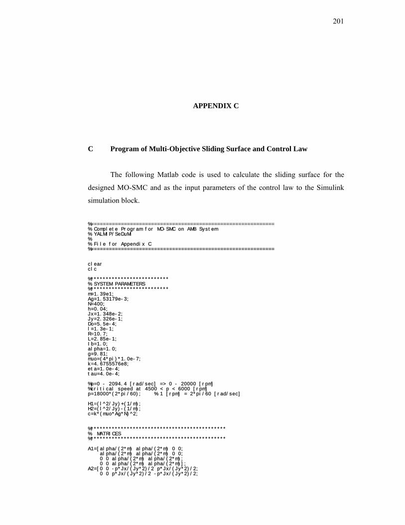
201

APPENDIX C

C Program of Multi-Objective Sliding Surface and Control Law

The following Matlab code is used to calculate the sliding surface for the

designed MO-SMC and as the input parameters of the control law to the Simulink

simulation block.

%============================================================= % Complete Program for MO-SMC on AMB System % YALMIP/SeDuMi % % File for Appendix C %============================================================= clear clc %************************** % SYSTEM PARAMETERS %************************** m=1.39e1; Ag=1.53179e-3; N=400; h=0.04; Jx=1.348e-2; Jy=2.326e-1; Do=5.5e-4; l=1.3e-1; R=10.7; L=2.85e-1; Ib=1.0; alpha=1.0; g=9.81; muo=(4*pi)*1.0e-7; k=4.6755576e8; eta=1.0e-4; tau=4.0e-4; %p=0 - 2094.4 [rad/sec] => 0 - 20000 [rpm] %critical speed at 4500 < p < 6000 [rpm] p=18000*(2*pi/60); % 1 [rpm] = 2*pi/60 [rad/sec] H1=(l^2/Jy)+(1/m); H2=(l^2/Jy)-(1/m); c=k*(muo*Ag*N)^2; %********************************************* % MATRICES %********************************************* A1=[alpha/(2*m) alpha/(2*m) 0 0; alpha/(2*m) alpha/(2*m) 0 0; 0 0 alpha/(2*m) alpha/(2*m); 0 0 alpha/(2*m) alpha/(2*m)]; A2=[0 0 -p*Jx/(Jy*2)/2 p*Jx/(Jy*2)/2; 0 0 p*Jx/(Jy*2)/2 -p*Jx/(Jy*2)/2;

202

p*Jx/(Jy*2)/2 -p*Jx/(Jy*2)/2 0 0; -p*Jx/(Jy*2)/2 p*Jx/(Jy*2)/2 0 0]; E4=zeros(4,4); I=eye(4,4); A=[E4 I; % Matrix A A1 A2]; B1=[254.3761 1.440 0 0; 1.440 254.3761 0 0; 0 0 254.3761 1.440; 0 0 1.440 254.3761]; B=[E4; % Matrix B B1]; C=[eye(4) zeros(4,4)]; %********************************************* % CONTROLLABILITY %********************************************* CTRB_RANK=rank(ctrb(A,B))-rank(A); % =0 (So (A,B) is controllable rank(ctrb(A,B)); rank(A); %********************************************* % TRANSFORM TO SPECIAL REGULAR FORM %********************************************* [n,m]=size(B); [Q,R]=qr(B); T=flipud(Q'); Bnew=T*B; B2=Bnew((n-m+1):n,:); T2=[eye(n-m) zeros((n-m),(n-m));zeros((n-m),(n-m)) inv(B2)]; T_complete=T2*T; % The transformation matrix % New transformed matrix Anew=T_complete*A*inv(T_complete); Bnew=T_complete*B; Cnew=C*inv(T_complete);

% Using 'SIGMA' test after % transformation

sys1=ss(A,B,C,0); % Original nominal system sys2=ss(Anew,Bnew,Cnew,0); % New transformed system subplot(2,1,1) sigma(sys1) title('SV for original system') subplot(2,1,2) sigma(sys2) title('SV for transformed system') A11=Anew(1:n-m,1:n-m); A12=Anew(1:n-m,n-m+1:n); A21=Anew(n-m+1:n,1:n-m); A22=Anew(n-m+1:n,n-m+1:n); B2=Bnew(n-m+1:n,1:m); %*********************************************** % DESIGN OF SLIDING SURFACE, S %*********************************************** alpha=-1000; % Controller parameters Qq=[15*eye(m) zeros(4,4)];%0.1*eye(m)]; Qj=Qq'*Qq; R=0.5*eye(4); theta=2*pi/9; % damping factor 2*pi/9 = 40degree p1=3500; % right vertical axis p2=50; [q,s]=size(Qq); At=Anew; % New System Bt=[-A12;alpha*eye(m)-A22]; %*********************************************** % DESIGN LMI VARIABLES %*********************************************** X1=sdpvar(n-m,n-m,'symmetric'); X2=sdpvar(m,m,'symmetric'); N1=sdpvar(m,n-m,'full'); Z=sdpvar(n,n,'symmetric');

203

X=blkdiag(X1,X2); N=[N1 X2]; %*********************************************** % DEFINING LMI TERMS %*********************************************** F=X>0; F=[F,[At*X+X*At'+Bt*N+(Bt*N)' X*Qq' N'*sqrt(R);Qq*X -eye(q) zeros(q,m); sqrt(R)*N zeros(m,q) -eye(m)]<0]; F=[F,[-Z (alpha*eye(n)-At)';(alpha*eye(n)-At) -X]<0]; F=[F,[(A11*X1+X1*A11'-A12*N1-N1'*A12')*sin(theta) (A11*X1-A12*N1-X1*A11'+N1'*A12')*cos(theta); (X1*A11'-N1'*A12'-A11*X1+A12*N1)*cos(theta) (A11*X1+X1*A11'-A12*N1-N1'*A12')*sin(theta)]<0]; F=[F,(A11*X1+X1*A11'-A12*N1-N1'*A12'+2*p2*X1)<0]; F=[F,(A11*X1+X1*A11'-A12*N1-N1'*A12'+2*p1*X1)>0]; %*********************************************** % CALL THE SOLVER %*********************************************** solvesdp(F,trace(Z)) Lt=double(N)*inv(double(X)) ; %Lt=N*X-1 (Eq. 29) M=double(N1)*inv(double(X1)); %M=N1*X1-1(Eq. --) S=S1*[M Im] Xout=eye(n,n)*double(X); L=Lt*(alpha*eye(n)-At); traceZ=trace(double(Z)); traceX=trace((alpha*eye(n)-At)'*inv(double(X))*(alpha*eye(n)-At)) sqrtX=sqrt(traceX); disp(sprintf('H2 cost is = %6.4e',sqrtX)) %*********************************************** % CONTROLLER PARAMETERS %*********************************************** K=-alpha*eye(m) S2=eye(m); S=[M S2]*T_complete'; SBinv=inv(S*B); SBK=SBinv*K; SA=S*A; Q=SBinv*SA; BS=B'*S'; rho=10.7; %ET=0.5; ET=0.0005; z=0.01; S %****************************** % TEST EIGENVALUES %****************************** Cl=A11-A12*M; Eig=eig(Cl)

MULTI-OBJECTIVE SLIDING MODE CONTROL OF ACTIVE …blog.uny.ac.id/mohkhairudin/files/2012/02/COMPLETE-THESIS.pdf · multi-objective sliding mode control of active magnetic bearing

Documents