Multi-objective due-date setting in a make-to-order environment

For Peer Review O

nly

MULTI-OBJECTIVE DUE DATE SETTING IN MAKE-TO-ORDER

ENVIRONMENT

Journal: International Journal of Production Research

Manuscript ID: TPRS-2008-IJPR-0812.R1

Manuscript Type: Original Manuscript

Date Submitted by the Author:

08-Jan-2009

Complete List of Authors: Sawik, Tadeusz; AGH University of Science and Technology, Dept of Operations Research and Information Technology

Keywords: DUE-DATE ASSIGNMENT, INTEGER PROGRAMMING, MAKE TO ORDER PRODUCTION, PRODUCTION PLANNING

Keywords (user): ROLLING PLANNING HORIZON

http://mc.manuscriptcentral.com/tprs Email: [email protected]

International Journal of Production Research

For Peer Review O

nlyMULTI-OBJECTIVE DUE DATE SETTING IN MAKE-TO-ORDER

ENVIRONMENT

Tadeusz Sawik

Department of Operations Research and Information Technology

AGH University of Science & Technology

Al.Mickiewicza 30, 30-059 Krakow, POLAND

tel.: +48 12 617 39 92

e-mail: [email protected]

Abstract:

This paper presents a new dual objective problem of due date setting over a rolling planning

horizon in make-to-order manufacturing and proposes a bi-criterion integer programming for-

mulation for its solution. In the proposed model the due date setting decisions are directly

linked with available capacity. A simple critical load index is introduced to quickly identify the

system bottleneck and the overloaded periods. The problem objective is to select maximal subset

of orders that can be completed by customer requested dates and to quote delayed due dates for

the remaining acceptable orders to minimize the number of delayed orders or the total number

of delayed products as a primary optimality criterion and to minimize total or maximum delay

of orders, as a secondary criterion. A weighted-sum program based on scalarization approach

is compared with a two-level due date setting formulation based on lexicographic approach. In

addition, a mixed integer programming model is provided for scheduling customer orders over

a rolling planning horizon to minimize maximum inventory level. Numerical examples mod-

eled after a real-world make-to-order flexible flowshop environment in the electronics industry

are provided and, for a comparison, the single-objective solutions that maximize total revenue

subject to service level constraints are reported.

Keywords:

Order acceptance; Due date setting; Make-to-order manufacturing; Rolling planning horizon;

Multi-objective integer programming.

Page 1 of 34

http://mc.manuscriptcentral.com/tprs Email: [email protected]

International Journal of Production Research

123456789101112131415161718192021222324252627282930313233343536373839404142434445464748495051525354555657585960

For Peer Review O

nly

1. Introduction

In make-to-order manufacturing accepting or rejecting customer orders is often combined

with due date setting. Accepting of too many orders with customer requested dates may

increase demand on capacity over available capacity and as a result may increase lead time

and decrease customer service level, i.e., more orders are delivered late after the requested

dates. To reduce the number of rejected or delayed orders, a manufacturer should quote due

dates for some orders later than the due dates requested by customers. Setting a due date

later than the requested date, however, may result in a reduction of revenue, whereas fulfilling

the order later than the quoted date may also result in loss of goodwill and sometimes even in

contractual penalty costs. On the other hand fulfilling the order earlier then the quoted date

may incur finished products inventory holding costs. Thus, the due date quoting problem

should account for the three costs (e.g. Hegedus and Hopp, 2001): cost for quoting a due date

later than requested date, cost for fulfilling the order later than the quoted date and finished

products inventory costs for fulfilling the order too early.

The order acceptance and due setting decisions can be made in either a real-time mode

or a batch mode. For real-time mode, a commitment due date is determined at the time of

the customer order arrival. For batch mode, customer orders are collected into a ”batch” and

subsequently considered together to determine the committed due dates for all orders in the

batch. While sometimes an initial due date quoting is made in real time, the batch mode

is commonly used in practice, e.g. in the e-business order fulfillment systems, as the actual

resource allocation and hard order commitment are carried out, see Chen et al. (2001).

The literature on order acceptance and due date setting is limited. An exact method for

selecting a subset of orders that maximizes revenues for the static problem in which all order

arrivals are known in advance is presented by Slotnick and Morton (1996), and Lewis and

Slotnick (2002) developed a dynamic programming approach for the multi-period case. A

mixed integer program for a quantity and due date quoting available to promise is presented

by Chen et al. (2001). Hegedus and Hopp (2001) consider order delay costs that measure the

positive difference between the quoted due date and the requested due date of an order.

The order acceptance strategies based on scheduling methods are presented by Wester et al.

(1992), Akkan (1997). In Wester et.al (1992) the decision whether or not to accept a new order

depends on how much order tardiness it will introduce to the system. Akkan (1997) suggests

to accept a new order if it can be included in the schedule such that it is completed by its

due date, and without changing the schedule for already accepted orders. Ebben et al. (2005)

developed a workload based acceptance strategy in a job shop environment. Corti et al. (2006)

propose a model supporting decision makers that have to verify the feasibility of customer

2

Page 2 of 34

http://mc.manuscriptcentral.com/tprs Email: [email protected]

International Journal of Production Research

123456789101112131415161718192021222324252627282930313233343536373839404142434445464748495051525354555657585960

For Peer Review O

nly

requested due dates. It adopts a capacity-driven approach to compare the capacity requested

by both potential and already confirmed orders with the actual level of available capacity.

Zorzini et al. (2008) investigate current practice supporting capacity and delivery lead-time

management in the capital goods sector based on a sample of fifteen Italian manufacturers

and propose a model to formalize the decision process for setting due dates in the selected

cases. Another approach is order acceptance based on revenue management principles, e.g.

Harris and Pinder (1995), Bertrand and van Ooijen (2000), Geunes et al.(2006).

This paper presents a new dual objective problem of due date setting over a rolling planning

horizon in make-to-order manufacturing, and proposes a bi-criterion integer programming

formulation for its solution. The problem objective is to select maximal subset of orders

that can be completed by customer requested dates and to quote delayed due dates for the

remaining acceptable orders to minimize the number of delayed orders or the total number

of delayed products as a primary optimality criterion and to minimize total or maximum

delay of orders, as a secondary criterion. The delay of order is defined to be the positive

difference between the due date committed by the manufacturer and the due date requested

by the customer. The two approaches: weighted-sum and lexicographic are proposed and

compared to a find optimal solutions for the bi-objective due date setting in make-to-order

flexible flowshop environment. Some possible enhancements of the basic models are discussed,

in particular, a revenue management approach is proposed to maximize total revenue subject

to service level constraints.

The major contribution of this paper is that it proposes a simple integer programming

approach to the bi-objective due date setting over a rolling planning horizon, in make-to-order

environment where the due date setting decisions are directly linked with available capacity.

The proposed model may prove its usefulness as a simple decision support tool for a rough-cut

capacity allocation in make-to-order environment. In particular, the proposed lexicographic

approach and a two-level decision making hierarchy with very small CPU time required to

find optimal solutions is capable of on-line supporting the due date setting decisions in the

dynamic make-to-order environment, where new computations are made every time a new

order arrives. In addition, a simple critical load index is introduced to quickly identify the

system bottleneck and the overloaded periods.

The paper is organized as follows. In the next section description of the due date setting

problem over a rolling planning horizon in a make-to-order flexible flowshop environment is

provided. The critical load index and some necessary conditions under which all due dates

can be met are presented in Section 3, and the proposed integer programming formulations for

the weighted-sum and the lexicographic approach are described in Section 4. A mixed integer

3

Page 3 of 34

http://mc.manuscriptcentral.com/tprs Email: [email protected]

International Journal of Production Research

123456789101112131415161718192021222324252627282930313233343536373839404142434445464748495051525354555657585960

For Peer Review O

nly

programming formulation for scheduling customer orders over a rolling planning horizon to

minimize maximum earliness of orders with respect to committed due dates is presented in

Section 5. Numerical examples modeled after a real-world make-to-order assembly system

and some computational results are provided in Section 6. Conclusions are made in the last

section.

2. Problem description

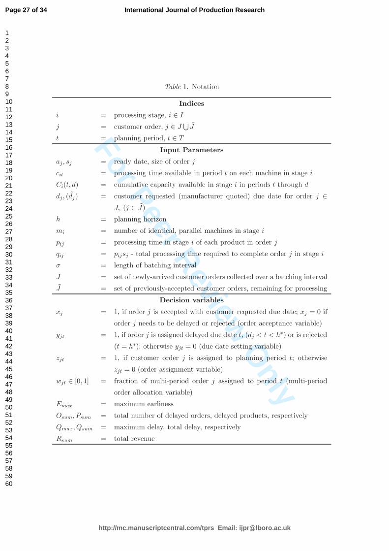
Table 1. Notation

The production system under study is a flexible flowshop that consists of m processing

stages in series, where each stage i ∈ I = {1, . . . ,m} is made up of mi ≥ 1 identical, parallel

machines. In the system various types of products are manufactured according to customer

orders, where each product type requires processing in various stages, however some products

may bypass some stages. The customer orders are single product type orders.

The order acceptance and due date setting decisions over a rolling planning horizon are

assumed to be made periodically upon arrivals of a number of orders in a specific time interval

(batching interval), given the set of already accepted orders remaining for processing and

the remaining available capacity. The batching interval consists of a fixed number of σ most

recent time periods (e.g. days) immediately preceding period t1, when the optimization model

is about to be executed, i.e. the model is executed every σ time periods at t1 = 1, 1 + σ, 1 +

2σ, 1 + 3σ, . . .. The problem objective is to plan activities for over a planning horizon, which

consists of the ensuing h (h > σ) time periods (e.g. working days) of equal length (e.g. hours

or minutes). Denote by T = {t1, . . . , t1 + h − 1} the set of planning periods covered in each

iteration.

Let J be the set of newly-arrived customer orders collected over a batching interval, and

J - the subset of previously-accepted orders remaining for processing, to be completed by

t1 + h − 1. (Notice that all previously-rejected orders are not considered any more.) Each

order j ∈ J (or j ∈ J) is described by a triple (aj , dj (or dj), sj (or sj)), where aj is the order

ready date (e.g. the earliest release period or the earliest period of material availability), dj

is the customer requested due date (e.g. customer required shipping date), dj ≤ t1 + h− 1 is

the due date of order j ∈ J committed by the manufacturer, sj is the size of order (required

quantity of ordered product type), and sj is the remaining order size.

Let pij ≥ 0 be the processing time in stage i of each product in order j, and let qij = pijsj

(or qij = pij sj) be the total processing time required to complete order j ∈ J (or j ∈ J)

4

Page 4 of 34

http://mc.manuscriptcentral.com/tprs Email: [email protected]

International Journal of Production Research

123456789101112131415161718192021222324252627282930313233343536373839404142434445464748495051525354555657585960

For Peer Review O

nly

in stage i. Denote by cit the total processing time available in period t on each machine

in stage i. The amount cit takes into account the flowshop configuration of the production

system and the production/transfer lot sizes. For each machine in stage i, cit must take into

account the time required for processing a single production lot at all upstream 1, . . . , i − 1

and downstream i+1, . . . ,m stages during the same planning period. As a result the available

capacity cit is smaller than simply the available machine hours in period t; cit can be bounded

as follows (see, Sawik 2007a):

ci ≤ cit ≤ ci, (1)

where

ci = L − maxj∈J

(∑

l∈I:l<i

bjplj) − maxj∈J

(∑

l∈I:l>i

bjplj),

ci = L − minj∈J

(∑

l∈I:l<i

bjplj) − minj∈J

(∑

l∈I:l>i

bjplj).

L is the length of each planning period (e.g. working hours per day) and bj is the produc-

tion/transfer lot size for order j (i.e., order quantity sj is split across multiple lots of size

bj).

When executing the model over time, after each batch execution, the remaining available

capacity is converted to fixed input for the next model run (see, (2)). The due date setting

decisions are made for a set J of newly-arrived customer orders collected over a batching

interval, given the remaining available capacity. The problem objective is to select maximal

subset of orders j ∈ J that can be completed by customer requested due dates and to quote

delayed due dates for the remaining acceptable orders to minimize the number of delayed

orders or delayed products as a primary optimality criterion and to minimize their total or

maximum delay, as a secondary criterion.

The two approaches are proposed. A monolithic approach, based on the weighted-sum

model where the order acceptance and the due dates setting are determined simultaneously,

and a hierarchical approach based on the lexicographic model, where first the maximal subset

of acceptable customer orders is selected and then delayed due dates are determined for

unrejected, acceptable orders to minimize their total or maximum delay.

3. Critical load index

In this section a simple critical load index is introduced and some necessary conditions are

derived for all customer orders to be accepted and for all requested due dates to be met.

5

Page 5 of 34

http://mc.manuscriptcentral.com/tprs Email: [email protected]

International Journal of Production Research

123456789101112131415161718192021222324252627282930313233343536373839404142434445464748495051525354555657585960

For Peer Review O

nly

Let Ci(t, d) be the remaining cumulative capacity available in stage i in periods t through

d, after deducting the capacity reserved for orders j ∈ J that were previously committed in

earlier model runs but whose production has not yet been completed, i.e.,

Ci(t, d) = mi

∑

τ∈T : t≤τ≤d

ciτ −∑

j∈J:t≤dj≤d

qij; d, t ∈ T : t ≤ d. (2)

A necessary condition to meet all customer requested due dates is that for each processing

stage i, each due date d ≤ t1 + h − 1 and each interval [t, d], t ∈ T : t ≤ d ending with d, the

demand on capacity does not exceed the available capacity, i.e., (Sawik 2007a)

Ψi(d) = maxt∈T :t≤d

(

∑

j∈J :t≤aj≤dj≤d qij

Ci(t, d)) ≤ 1; d ∈ T, i ∈ I (3)

where Ψi(d) is the cumulative capacity ratio for due date d with respect to processing stage i.

If Ψi(d) ≤ 1, then for any period t ≤ d the cumulative demand on capacity in stage i of

all the orders with due dates not greater than d and ready dates not less than t (numerator

in (3)) does not exceed the cumulative capacity available in this stage in periods t through d

(denominator in (3)).

When Ψi(d) > 1, then at least one order to be processed at stage i, with requested due

date not later than d must be delayed or rejected (if d = t1 +h−1) to meet available capacity

constraints.

If all customer orders were continuously allocated among the consecutive time periods so

that all periods could be filled exactly to their capacities, the necessary condition (3) could

become sufficient for all orders to be completed by their due dates. Denote by Ψ(d) the

cumulative capacity ratio for due date d

Ψ(d) = maxi∈I

Ψi(d); d ∈ T. (4)

The ratio Ψ(d), d ∈ T can be used as a simple critical load index to identify the bottleneck

stages and the overloaded periods.

Notice that if all customer orders are ready at the beginning of planning horizon, (aj =

t1 ∀j ∈ J), then Ψ(t1 + h − 1) is the cumulative capacity ratio for the entire horizon, i.e.,

the total capacity ratio. A necessary condition to have a feasible production schedule with all

customer orders completed during the planning horizon is that the total capacity ratio is not

greater than one

maxi∈I

∑

j∈J qij

Ci(t1, t1 + h − 1)≤ 1 (5)

The basic due date setting problem presented in the next section is applied for orders with

requested due dates such that condition (3) is not satisfied. In this case the proposed model

6

Page 6 of 34

http://mc.manuscriptcentral.com/tprs Email: [email protected]

International Journal of Production Research

123456789101112131415161718192021222324252627282930313233343536373839404142434445464748495051525354555657585960

For Peer Review O

nly

determines new, delayed due dates to satisfy (3) and, in addition, to reach some optimality

criteria. If, however, condition (3) holds for all customer requested due dates, then the due

dates can be met and the due date setting problem becomes trivial and need not to be

considered.

4. Bi-objective due date setting

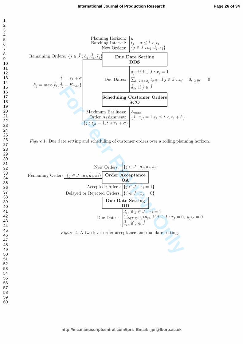
Figure 1. Due date setting and scheduling of customer orders over a rolling planning horizon.

In this section integer programming formulations are proposed for the bi-objecive due

date setting over a rolling planning horizon (Fig. 1). The two sets of the integer programs are

proposed: a weighted-sum program DDS, based on scalarization approach, and a hierarchy

of two programs OA and DD, based on lexicographic approach.

The primary objective of the due date setting problem is to maximize the customer service

level, that is to minimize the number of delayed orders Osum, i.e., the orders for which the

committed due dates are later than the customer requested dates. Minimization of the number

of delayed orders may often lead to a large number of delayed products since a high customer

service level can be achieved by setting later due dates for a small number of large size

customer orders. Therefore, an alternative primary objective is to minimize the number of

delayed products Psum.

Similarly, the two alternative secondary objective functions are considered: minimum

of the total delay Qsum of all orders or minimum of the maximum delay Qmax among all

orders, where the order delay is defined as the positive difference between the committed

and the requested due date. While minimization of Qsum aims at reducing the total delay

of all postponed customer orders, minimization of Qmax gives preference to reduction of the

maximum delay with respect to requested due date of each individual order.

The orders that cannot be accepted in periods t1 through t1 + h − 1 due to insufficient

capacity and hence should be rejected are assigned at a significant penalty to a dummy

planning period h∗ = t1 + h with infinite capacity. Let T ∗ = T⋃

{t1 + h} = {t1, . . . , t1 + h −

1, t1 + h} be the enlarged set of planning periods with a dummy period h∗ = t1 + h included.

The following two basic decision variables are introduced in the proposed integer program-

ming models (for notation used, see Table 1).

• Order acceptance variable: xj = 1, if order j is accepted with its requested due date or

xj = 0 if order j needs to be delayed or rejected,

7

Page 7 of 34

http://mc.manuscriptcentral.com/tprs Email: [email protected]

International Journal of Production Research

123456789101112131415161718192021222324252627282930313233343536373839404142434445464748495051525354555657585960

For Peer Review O

nly

• Due date setting variable: yjt = 1, if order j is assigned delayed due date t (dj < t < h∗),

or is rejected (t = h∗); otherwise yjt = 0.

Now, the primary and the secondary objective functions f1 and f2 can be expressed as

below.

f1 ∈ {Osum, Psum} (6)

f2 ∈ {Qsum, Qmax} (7)

where

Osum =∑

j∈J

(1 − xj − yjh∗) (8)

Psum =∑

j∈J

sj(1 − xj − yjh∗) (9)

Qsum =∑

j∈J,t∈T :t>dj

(t − dj)yjt (10)

Qmax = maxj∈J,t∈T :t>dj

(t − dj)yjt (11)

Model DDS: Due date setting to minimize weighted sum of delayed orders or delayed

products and total or maximum delay

Minimize

λ0

∑

j∈J

yjh∗ + λ1f1 + λ2f2 (12)

where λ0 ≫ λ1 ≥ λ2

subject to

1. Order acceptance or due date setting constraints:

- each customer order is either accepted with its requested due date, is assigned a delayed

due date or is rejected,

xj +∑

t∈T ∗:t>dj

yjt = 1; j ∈ J (13)

2. Capacity constraints:

- for any period t ≤ d, the cumulative demand on capacity in stage i of all orders accepted

with requested (or delayed) due dates not greater than d and ready dates (or requested due

dates, respectively) not less than t must not exceed the cumulative capacity available in this

stage in periods t through d

∑

j∈J : t≤aj≤dj≤d

qijxj +∑

j∈J

∑

τ∈T : t≤dj<τ≤d

qijyjτ ≤ Ci(t, d); d, t ∈ T, i ∈ I : t ≤ d (14)

8

Page 8 of 34

http://mc.manuscriptcentral.com/tprs Email: [email protected]

International Journal of Production Research

123456789101112131415161718192021222324252627282930313233343536373839404142434445464748495051525354555657585960

For Peer Review O

nly

3. Maximum delay constraints (if f2 = Qmax):

- for each delayed order j with adjusted due date t > dj , its delay (t − dj) cannot exceed

the maximum delay Qmax,

(t − dj)yjt ≤ Qmax; j ∈ J, t ∈ T : t > dj (15)

Qmax ≥ 0 (16)

4. Integrality conditions

xj ∈ {0, 1}; j ∈ J (17)

yjt ∈ {0, 1}; j ∈ J, t ∈ T ∗ : t > dj . (18)

In the objective function (12), λ1 ≥ λ2 as the primary objective of DDS is to minimize

the number of delayed orders f1 = Osum (8) or alternatively to minimize total number of

delayed products f1 = Psum (9), delivered after the customer requested dates. The objective

function is additionally penalized with λ0 ≫ λ1 for each rejected order.

Model DDS for due date setting determines feasible due dates using the capacity con-

straint (14), which is based on condition (3) for the feasibility of customer requested due

dates. (13) and (14) ensure that each accepted order j ∈ J (such that yjh∗ = 0) is completed

on or before its requested due date dj (if xj = 1) or on its delayed due date t > dj (if xj = 0

and yjt = 1). If condition (3) holds for all customer requested due dates, then the due date

setting problem DDS becomes trivial and the objective function (12) takes on zero value,

since xj = 1 ∀j ∈ J and yjt = 0 ∀j ∈ J, t ∈ T ∗. Otherwise, delayed due dates are determined

for some customer orders.

The solution to the integer program DDS determines the maximal subset {j ∈ J : xj = 1}

of customer orders accepted with the customer requested due dates dj and the subsets of

remaining orders: {j ∈ J : xj = 0, yjh∗ = 0} - delayed orders and {j ∈ J : xj = 0, yjh∗ = 1}

- rejected orders.

Denote by Dj , the requested or delayed due date for each newly-arrived and accepted

order j ∈ J , or committed due date for each previously-accepted order j ∈ J remaining for

processing, i.e.,

Dj =

dj if j ∈ J : xj = 1∑

t∈T :t>djtyjt if j ∈ J : xj = 0, yjh∗ = 0

dj if j ∈ J

(19)

9

Page 9 of 34

http://mc.manuscriptcentral.com/tprs Email: [email protected]

International Journal of Production Research

123456789101112131415161718192021222324252627282930313233343536373839404142434445464748495051525354555657585960

For Peer Review O

nly

4.1. Lexicographic approach

Since λ1 ≥ λ2 in the objective function (12), a lexicographic approach can also be applied

to solve the bi-objective integer program DDS. Then DDS can be replaced by the following

two integer programs OA and DD to be solved sequentially (see, Fig. 2).

Figure 2. A two-level order acceptance and due date setting.

Model OA: Order acceptance to minimize number of delayed /rejected orders or

delayed/rejected products

Minimize

f1 (20)

subject to

1. Capacity constraints:

- for any period t ≤ d, the cumulative demand on capacity in stage i of all accepted

orders with due dates not greater than d and ready dates not less than t must not exceed the

cumulative capacity available in this stage in periods t through d

∑

j∈J : t≤aj≤dj≤d

qijxj ≤ Ci(t, d); d, t ∈ T, i ∈ I : t ≤ d (21)

2. Integrality conditions: (17)

The solution to OA determines the minimal subset J0 = {j ∈ J : xj = 0} of delayed

or rejected orders. New, delayed due dates for acceptable orders are determined using the

integer program presented below.

Model DD: Due date setting for delayed orders to minimize total or maximum delay

Minimize

f2 + h∑

j∈J0

yj,h∗ (22)

subject to

1. Due date assignment constraints:

- each order is either assigned a due date later than its requested due date or is rejected,

∑

t∈T ∗:t>dj

yjt = 1; j ∈ J0 (23)

10

Page 10 of 34

http://mc.manuscriptcentral.com/tprs Email: [email protected]

International Journal of Production Research

123456789101112131415161718192021222324252627282930313233343536373839404142434445464748495051525354555657585960

For Peer Review O

nly

2. Capacity constraints:

- for any period t ≤ d, the cumulative demand on capacity in stage i of all accepted orders

with requested due dates not greater than d and ready dates not less than t, and of all delayed

orders with adjusted due dates not greater than d and requested due dates not less than t

must not exceed the cumulative capacity available in this stage in periods t through d

∑

j∈J0

∑

τ∈T : t≤dj<τ≤d

qijyjτ ≤ Ci(t, d) −∑

j∈J\J0: t≤aj≤dj≤d

qij ; d, t ∈ T, i ∈ I : t ≤ d (24)

3. Maximum delay constraints (if f2 = Qmax): (15), (16)

4. Integrality conditions: (18).

The objective function (22) is penalized with h periods of delay for each rejected order.

Notice, that if multiple optima (alternative minimal sets J0 of delayed and rejected orders)

exist for the top level problem OA, then the base level problem DD (where a single set

J0 is applied only) may produce weakly non-dominated solutions with f2 greater than those

obtained by parameterizing on λ the weighted-sum program DDS. On the other hand, it is

well known, that the non-dominated solution set of a multi-objective integer program such as

DDS cannot be fully determined even if the complete parameterization on λ is attempted,

e.g. Steuer (1986).

In order to eliminate the weakly non-dominated solutions, the secondary objective function

f2 should be minimized over the solutions that minimize the primary objective function f1.

Then, the constraint set of the base level problem DD should be replaced by the constraints of

DDS with additional upper bound f1 ≤ f∗1 on the corresponding primary objective function

(8) or (9), where f∗1 is the optimal solution value to the top level problem OA.

4.2. Model enhancements

The models presented in this section can be modified or enhanced to consider additional

features of the due date setting problem that can be met in practice. A few possible extensions

of the models are proposed below.

1. Modified objective functions.

• Maximization of total revenue.

The sales departments often apply revenue management principles for order selec-

tion and due date setting. The objective is to maximize a revenue function, e.g.,

to maximize

11

Page 11 of 34

http://mc.manuscriptcentral.com/tprs Email: [email protected]

International Journal of Production Research

123456789101112131415161718192021222324252627282930313233343536373839404142434445464748495051525354555657585960

For Peer Review O

nlyRsum =

∑

j∈J

rjsjxj +∑

j∈J,t∈T :t>dj

rjtsjyjt −∑

j∈J

r∗j sjyjh∗, (25)

where rj = rj,djand rjt is per unit revenue for order j accepted with customer

requested due date dj and for order j with delayed due date t > dj, respectively.

For rejected orders r∗j is per unit loss of revenue.

Most often customer value short lead times (due dates) over long lead times. Setting

delayed due dates results in reduction of revenue. The revenue declines with an

increase in the delay of committed due dates with respect to requested due dates,

i.e.,

rjt > rj,t+1, t ∈ T, t ≥ dj .

We assume that setting delayed due date results in reduction of revenue propor-

tional to the delay, e.g. Bertrand and van Ooijen (2000). Per unit revenue rjt

decreases by some percent for each day of delay (t− dj) of delivery with respect to

customer requested date dj , for example

rjt = rj(1 − αj(t − dj)); t ≥ dj,

where 0 < αj < 1 is the rate of daily loss of revenue for order j.

In addition, a fixed loss βjrj (0 < βj < 1) of revenue may be applied for each

delayed product in order j, i.e.

rjt = rj(1 − βj − αj(t − dj)); t > dj .

2. Minimum service level required.

If minimization of the number of delayed orders is replaced by another objective function,

e.g. maximization of total revenue (25), then the following constraint should be added

to the modified model to maintain required service level γ, 0 < γ ≤ 1, where γ is the

fraction of non delayed customer orders.

∑

j∈J

xj ≥ γn (26)

3. Nonnegotiable customer due dates.

Some customers specify requested due date that cannot be delayed. Let JN ⊂ J be

the subset of customer orders with nonnegotiable due dates. A feasible solution must

satisfy the following constraints

xj = 1; j ∈ JN (27)

12

Page 12 of 34

http://mc.manuscriptcentral.com/tprs Email: [email protected]

International Journal of Production Research

123456789101112131415161718192021222324252627282930313233343536373839404142434445464748495051525354555657585960

For Peer Review O

nly

4. Customer due date windows.

Customer specifies a delivery time window, e.g., acceptable latest delay of shipping date

δjmax, j ∈ J . Then, the integer programs must include the following constraints

tyjt ≤ dj + δjmax; j ∈ J, dj < t ≤ djmax (28)

5. Rush orders.

For urgent orders a high priority πj > 1 can be introduced in the objective function,

e.g.,

λ0

∑

j∈J

πjyjh∗ + λ1

∑

j∈J

πj(1 − xj − yjh∗) + λ2

∑

j∈J,t∈T :t>dj

πj(t − dj)yjt (29)

where λ0 ≫ λ1 ≥ λ2, and πj = 1 for regular orders.

6. Real-time mode.

The proposed integer programs can be applied in real-time mode upon arrival of each new

order, given the set of already accepted orders waiting for processing and the remaining

available capacity. In particular, the lexicographic approach that does not require as

much computation time as the weighted-sum approach (see Section 6) is capable of

quoting due date in real-time mode for each new order.

5. Scheduling customer orders

Model DDS (or a hierarchy of models OA and DD) is executed over a rolling planning horizon

every σ time periods (the length of batching interval) to quote due dates for all newly-arrived

orders j ∈ J collected over the most recent batching interval, given the previously-accepted

orders j ∈ J remaining for processing. When simulating the execution of model DDS over

time, the set j ∈ J of previously-accepted orders remaining for processing must be determined

for each model run, which requires detailed scheduling of customer orders to be performed

over a rolling planning horizon, e.g. Smutnicki (2007).

In this section the mixed integer program SCO is presented for a non-delayed scheduling

of customer orders over a rolling planning horizon. The scheduling objective is to find an

assignment of orders to periods over the horizon such that each order is assigned not later

than its committed due date and the maximum earliness with respect to the due date among

all orders is minimized.

The following two types of customer orders are considered:

13

Page 13 of 34

http://mc.manuscriptcentral.com/tprs Email: [email protected]

International Journal of Production Research

123456789101112131415161718192021222324252627282930313233343536373839404142434445464748495051525354555657585960

For Peer Review O

nly

1. Small-size, indivisible orders, where each order can be fully processed in a single time

period. The small size orders are referred to as single-period orders.

2. Large-size, divisible orders, where each order cannot be completed in one period and

must be split into single-period portions to be processed in a subset of consecutive time

periods. The large size orders are referred to as multi-period orders.

In practice, two types of customer orders are simultaneously scheduled. Denote by J1 ⊆

J , and J2 ⊆ J , respectively the subset of newly-arrived indivisible and divisible orders,

respectively, where J1⋃

J2 = J , and J1⋂

J2 = ∅.

The basic decision variable for scheduling customer orders is order assignment variable

zjt, where zjt = 1, if customer order j is assigned to planning period t; otherwise zjt = 0.

In addition, order allocation variable wjt is required to schedule multi-period orders, where

wjt ∈ [0, 1] denotes a fraction of a multi-period order j assigned to period t.

Let J = J1⋃

J2′⋃ ˜J2′′ be the set of previously-accepted orders, where J1, J2′ and ˜J2′′

is the subset of previously-accepted single-period orders waiting for processing, the subset of

previously-accepted multi-period orders waiting for processing and the subset of previously-

accepted and uncompleted multi-period orders remaining for completion, respectively.

It is assumed that the allocation over time of uncompleted multi-period orders j ∈ ˜J2′′

(i.e., such that 0 <∑

t<t1 wjt < 1) remains unchanged, that is,

wjt = wjt, zjt = zjt; j ∈ ˜J2′′, t < t1 + h,

where wjt and zjt are the assignments and the allocation of uncompleted multi-period orders

determined at the previous run of the scheduling model.

Model SCO: Scheduling customer orders to minimize maximum earliness

Minimize

Emax (30)

subject to

1. Order non-delayed assignment constraints

- each single-period order is assigned to exactly one planning period not later than its due

date,

∑

t∈T : aj≤t≤Dj

zjt = 1; j ∈ J1⋃

J1 (31)

14

Page 14 of 34

http://mc.manuscriptcentral.com/tprs Email: [email protected]

International Journal of Production Research

123456789101112131415161718192021222324252627282930313233343536373839404142434445464748495051525354555657585960

For Peer Review O

nly

- each multi-period order waiting for processing is assigned to a subset of consecutive

planning periods not later than its due date,

zj⌊(τ1+τ2)/2⌋ ≥ zjτ1 + zjτ2 − 1; j ∈ J2⋃

J2′, τ1, τ2 ∈ T : aj ≤ τ1 < τ2 ≤ Dj (32)

2. Order allocation constraints

- each order waiting for processing must be completed not later than its due date,

∑

t∈T :aj≤t≤Dj

wjt = 1; j ∈ J⋃

J1⋃

J2′ (33)

- each single-period order is completed in a single period,

zjt = wjt; j ∈ J1⋃

J1, t ∈ T : aj ≤ t ≤ Dj (34)

- each multi-period order waiting for processing is allocated among all the periods that

are selected for its assignment,

wjt ≤ zjt; j ∈ J2⋃

J2′, t ∈ T : aj ≤ t ≤ Dj (35)

4. Capacity constraints

- in every period the demand on capacity at each assembly stage cannot be greater than

the capacity available in this period,

∑

j∈J⋃

J

pijsjwjt ≤ micit; i ∈ I, t ∈ T (36)

5. Maximum earliness constraints

- for each early order j assigned to period t < Dj, its earliness (Dj − t) cannot exceed the

maximum earliness Emax to be minimized,

(Dj − t)zjt ≤ Emax; j ∈ J⋃

J1⋃

J2′, t ∈ T : aj ≤ t ≤ Dj (37)

6. Fixed allocation constraints

- the allocation of each uncompleted multi-period order remains unchanged,

wjt = wjt; j ∈ ˜J2′′, t ∈ T (38)

zjt = zjt; j ∈ ˜J2′′, t ∈ T (39)

7. Nonnegativity and integrality conditions

wjt ∈ [0, 1]; j ∈ J⋃

J , t ∈ T : aj ≤ t ≤ Dj (40)

zjt ∈ {0, 1}; j ∈ J⋃

J , t ∈ T : aj ≤ t ≤ Dj (41)

Emax ≥ 0, integer. (42)

15

Page 15 of 34

http://mc.manuscriptcentral.com/tprs Email: [email protected]

International Journal of Production Research

123456789101112131415161718192021222324252627282930313233343536373839404142434445464748495051525354555657585960

For Peer Review O

nly

If single- and two-period orders are considered only, then (31) can be replaced by the

following constraints to guarantee that each order is assigned to at most two consecutive

periods,

zjt + zjt+1 ≤ 2; j ∈ J2⋃

J2′, t ∈ T : aj ≤ t < Dj (43)

zjt + zjt′ ≤ 1; j ∈ J2⋃

J2′, t ∈ T, t′ ∈ T : aj ≤ t < Dj − 1, t′ ≥ t + 2 (44)

The objective (30) minimizes the maximum earliness Emax (36) among all customer orders

or equivalently the maximum difference between order due date and its assignment period such

that no tardiness of the customer orders with respect to committed due dates is ensured. The

resulting assignment period can be considered to be the latest period of delivery the required

parts such that no tardiness of orders is ensured. If for some customer orders the required

parts were delivered later than Emax periods ahead of the due date, i.e., later than in period

max{t1,Dj−Emax} the limited order earliness due to the later parts availability could restrict

a reallocation of the orders to the earlier periods with surplus of capacity. In a consequence,

tardy orders or even infeasible schedules could occur, with some customer orders unscheduled

during the planning horizon.

An implicit objective of SCO is to minimize the maximum level of total input inventory

of parts waiting for assembly and the finished products waiting for delivery to the customers,

see Sawik (2007b). To minimize the maximum level of total input and output inventory, the

ready date aj of each customer order j ∈ J⋃

J for each run of model DDS can be replaced

by the the latest delivery date of the required parts, i.e.,

aj = max{t1,Dj − Emax} (45)

Model SCO is executed over a rolling planning horizon every σ time periods. The solution

to the mixed integer program SCO determines the assignment of customer orders to planning

periods t ∈ [t1, t1 + h) over the current planning horizon and by this the production schedule

for customer orders assigned to periods in the next batching interval [t1, t1+σ−1]. As a result,

the solution to SCO determines the set J = {j : zjt = 1, t1 + σ ≤ t < t1 + h} of customer

orders assigned to periods [t1 + σ, t1 + h), i.e., the set of orders remaining for processing over

the next planning horizon and hence required for the next run of model DDS, see Fig. 1.

5.1. Scheduling single-period orders

The mixed integer program SCO for assignment of single-and multi-period orders can be

simplified when only single-period orders are considered. Then, the order allocation variables

16

Page 16 of 34

http://mc.manuscriptcentral.com/tprs Email: [email protected]

International Journal of Production Research

123456789101112131415161718192021222324252627282930313233343536373839404142434445464748495051525354555657585960

For Peer Review O

nly

wjt are not required any more and model SCO for single-period orders can be rewritten as

below.

Model SCO1: Scheduling single-period orders

Minimize (30)

subject to

1. Order non-delayed assignment constraints: (31)

2. Capacity constraints

∑

j∈J⋃

J

pijsjzjt ≤ micit; i ∈ I, t ∈ T (46)

4. Maximum earliness constraints: (37)

5. Integrality conditions: (41), (42).

6. Computational examples

In this section some computational examples are presented to illustrate possible applications

of the proposed approach. The examples are modeled after a real world distribution center

for high-tech products, where finished products are assembled for shipping to customers.

The distribution center is a flexible flowshop made up of six processing stages with parallel

machines. The customer orders require processing in at most four stages: 1, 2, 3 or 4 or 5,

and 6. All customer orders are single-period and single-product type orders.

A brief description of the production system, production process, products and the cus-

tomer orders is given below.

1. Production system

• six processing stages: 10 parallel machines in each stage i = 1, 2; 20 parallel ma-

chines in each stage i = 3, 4, 5; and 10 parallel machines in stage i = 6.

2. Products

• 10 product types of three product groups, each to be processed on a separate group

of machines (in stage 3 or 4 or 5),

3. Processing times (in seconds) for product types:

product type/stage 1 2 3 4 5 6

1 20 0 120 0 0 15

17

Page 17 of 34

http://mc.manuscriptcentral.com/tprs Email: [email protected]

International Journal of Production Research

123456789101112131415161718192021222324252627282930313233343536373839404142434445464748495051525354555657585960

For Peer Review O

nly

2 20 0 140 0 0 15

3 10 0 160 0 0 10

4 15 5 0 120 0 15

5 15 10 0 140 0 15

6 10 5 0 160 0 10

7 15 10 0 180 0 15

8 20 5 0 0 120 15

9 15 0 0 0 140 10

10 15 0 0 0 160 10

4. The length of planning period (one production day): 2 × 8 = 16 hours.

5. The length of batching interval: σ = 5 days.

6. Planning horizon: h = 20 days.

In the computational experiments the models DDS and SCO1 were executed three times

over a rolling planning horizon to quote due dates for orders collected over the three batching

intervals:

• In period t1 = 1, the due dates ranging from period 1 to period 20 are quoted for 641

customer orders collected over the first batching interval, before period 1.

• In period t1 = 6, the due dates ranging from period 6 to period 25 are quoted for 75

customer orders collected over the second batching interval [1,5].

• In period t1 = 11, the due dates ranging from period 11 to period 30 are quoted for 92

customer orders collected over the third batching interval [6,10].

The total of 808 orders are considered over the entire planning horizon [1,30], each ranging

from 5 to 9700 products of a single type. The total demand for all products is 551965. For the

input data the necessary condition (5) to have a feasible schedule with all orders completed

during the planning horizon is satisfied, and hence no order needs to be rejected. Furthermore,

the input data indicates that stage 2 has significant over capacity and stage 3, 4 and 5 are

bottlenecks.

Each run of the models DDS and SCO1 assigns orders to planning periods over a 20

time-period horizon, which corresponds to the assumption that resource availability is fixed

for 20 planning periods in the future. These resources can be reassigned in subsequent runs,

i.e. for a σ = 5 days long batching interval, the first and the second runs overlap in 15 time

18

Page 18 of 34

http://mc.manuscriptcentral.com/tprs Email: [email protected]

International Journal of Production Research

123456789101112131415161718192021222324252627282930313233343536373839404142434445464748495051525354555657585960

For Peer Review O

nly

periods and some order assignments set in the first run can be changed in the second run

(subject to the constraint that committed order due dates remain unchanged.)

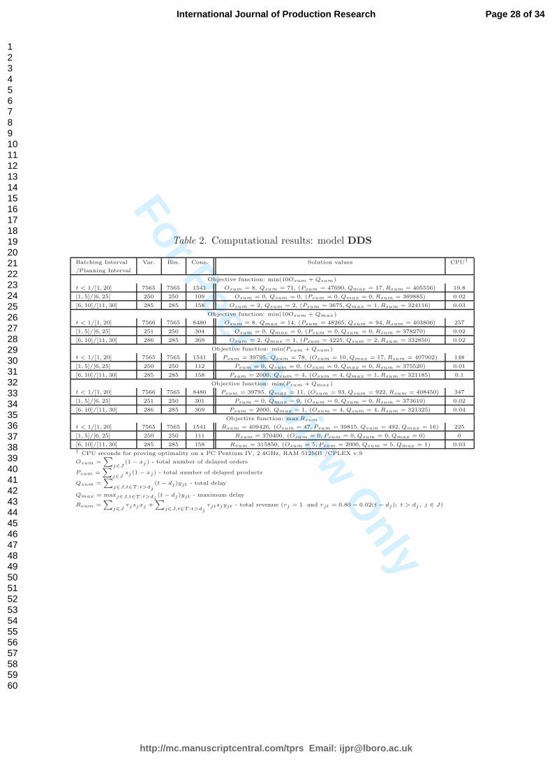
Table 2. Computational results: model DDS

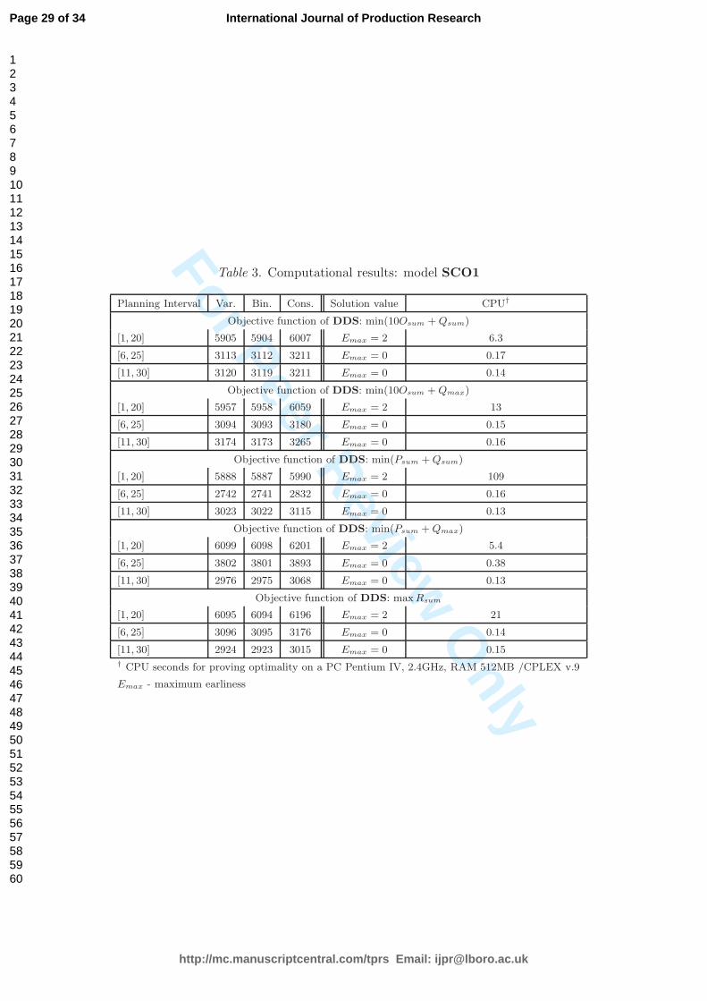
Table 3. Computational results: model SCO1

Table 4. Computational results: ex-post solutions

In the computational experiments a single solution to DDS is sought for the weights

λ1 ≥ λ2, selected as nonnegative integers. The main purpose of using such weights is to obtain

the integer-valued objective function (11), which leads to the reduced CPU time required to

find proven optimal solution of DDS.

The characteristics of integer program DDS for various objective functions and for the

subsequent batching and planning intervals are summarized in Table 2. The size of the integer

program is represented by the total number of variables, Var., number of binary variables,

Bin., and number of constraints, Cons. Table 2 presents solution values Osum or Psum of the

primary objective function f1, respectively with λ1 = 10 or λ1 = 1 in (12), and Qsum or Qmax

of the secondary objective function f2 with λ2 = 1 in (12). Finally, the last column shows

CPU time in seconds required to prove optimality of the solution. In addition, the last part

of Table 2 presents solution results with maximum revenue Rsum (25). All solution values

are presented along with the corresponding counter values of the complementary objective

functions (in parenthesis).

Table 2 indicates that optimal values for the primary objective functions Osum or Psum

are identical for different secondary objective functions Qsum and Qmax of the corresponding

solutions. In order to reach feasibility, the surplus of demand exceeding available capacity

in the beginning periods has been reallocated to later periods with excess of capacity in a

similar way for both the secondary criteria. However, the overall solution for the secondary

objective function f2 = Qsum outperforms that obtained for f2 = Qmax; f2 = Qsum leads to

less delayed products, a higher revenue, and a better complementary value of Qmax, than the

complementary value of Qsum for f2 = Qmax.

Furthermore, Table 2 demonstrates that for the customer orders collected in the second

batching interval [1,5] all requested due dates are acceptable, i.e. condition (3) holds over the

planning horizon [6,25], and hence the execution of model DDS was not necessary.

The characteristics of the integer program SCO1 for scheduling customer orders and

19

Page 19 of 34

http://mc.manuscriptcentral.com/tprs Email: [email protected]

International Journal of Production Research

123456789101112131415161718192021222324252627282930313233343536373839404142434445464748495051525354555657585960

For Peer Review O

nly

the solution results are summarized in Table 3. For all objective functions of DDS, model

SCO1 yields identical maximum earliness Emax = 2, Emax = 0 and Emax = 0 for subsequent

planning horizons, respectively [1,20], [6,25] and [11,30]. The results indicate that for the

example considered, all customer orders in the second and the third rolling planning horizon

can be completed on due dates (requested or committed).

Notice, that in the computational experiments the number of customer orders collected

before period t = 1 is much greater than those collected over the subsequent batching intervals.

As a result, the integer programs DDS and SCO1 for the the first interval [1,20] of the rolling

planning horizon have the greatest size.

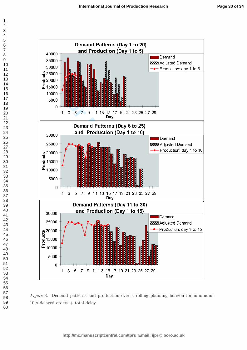
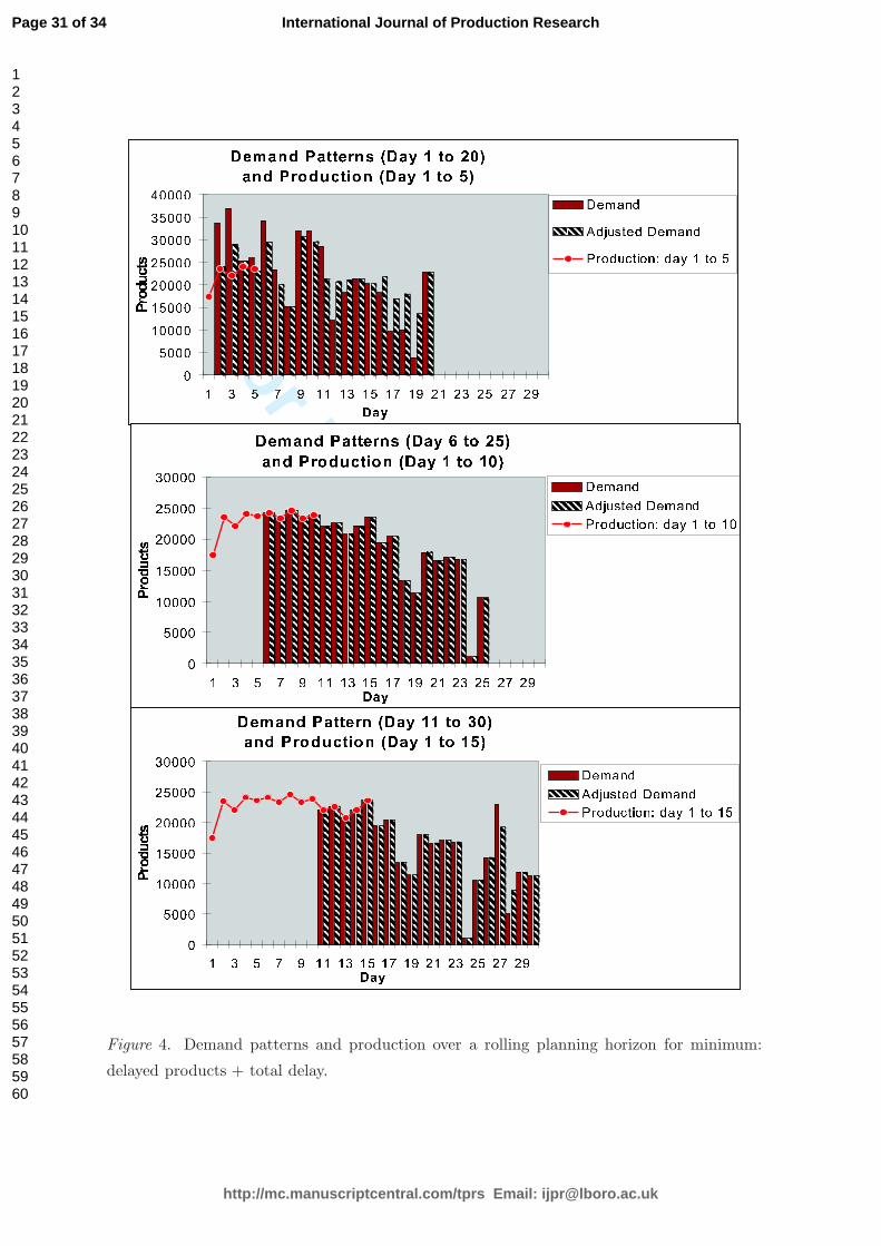
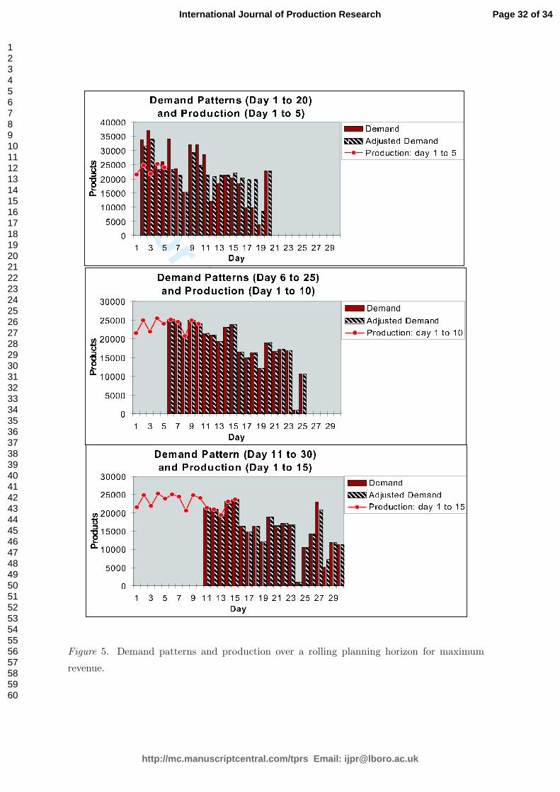
Demand patterns and the aggregated production schedule over a rolling planning horizon

for various objective functions are shown in Fig. 3-5. Notice similar adjusted demand patterns

for min(Psum + Qsum) (Fig. 4) and for maxRsum (Fig. 5).

Figure 3. Demand patterns and production over a rolling planning horizon for minimum:

10 x delayed orders + total delay.

Figure 4. Demand patterns and production over a rolling planning horizon for minimum:

delayed products + total delay.

Figure 5. Demand patterns and production over a rolling planning horizon for maximum

revenue.

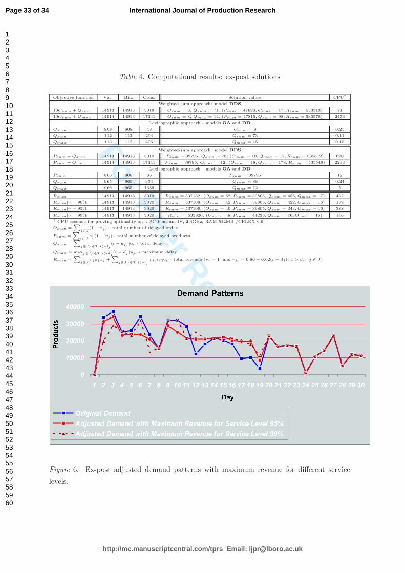
For a comparison, Table 4 presents ex-post solution results for various objective func-

tions, obtained when the demand is known ahead of time for the entire monthly horizon. In

particular, Table 4 presents ex-post solutions for the objective of maximizing total revenue

(25) subject to service level constraints (26). The resulting demand patterns are shown in

Fig. 6. The comparison of the ex-post solutions (Table 4) with the corresponding results on

the rolling horizon basis (Table 2) demonstrates that both the total number of delayed orders

and the total number of delayed products are smaller for the ex-post solutions. The more

demand-pattern information is offered, i.e. the longer is the batching interval, the better

solution results are obtained.

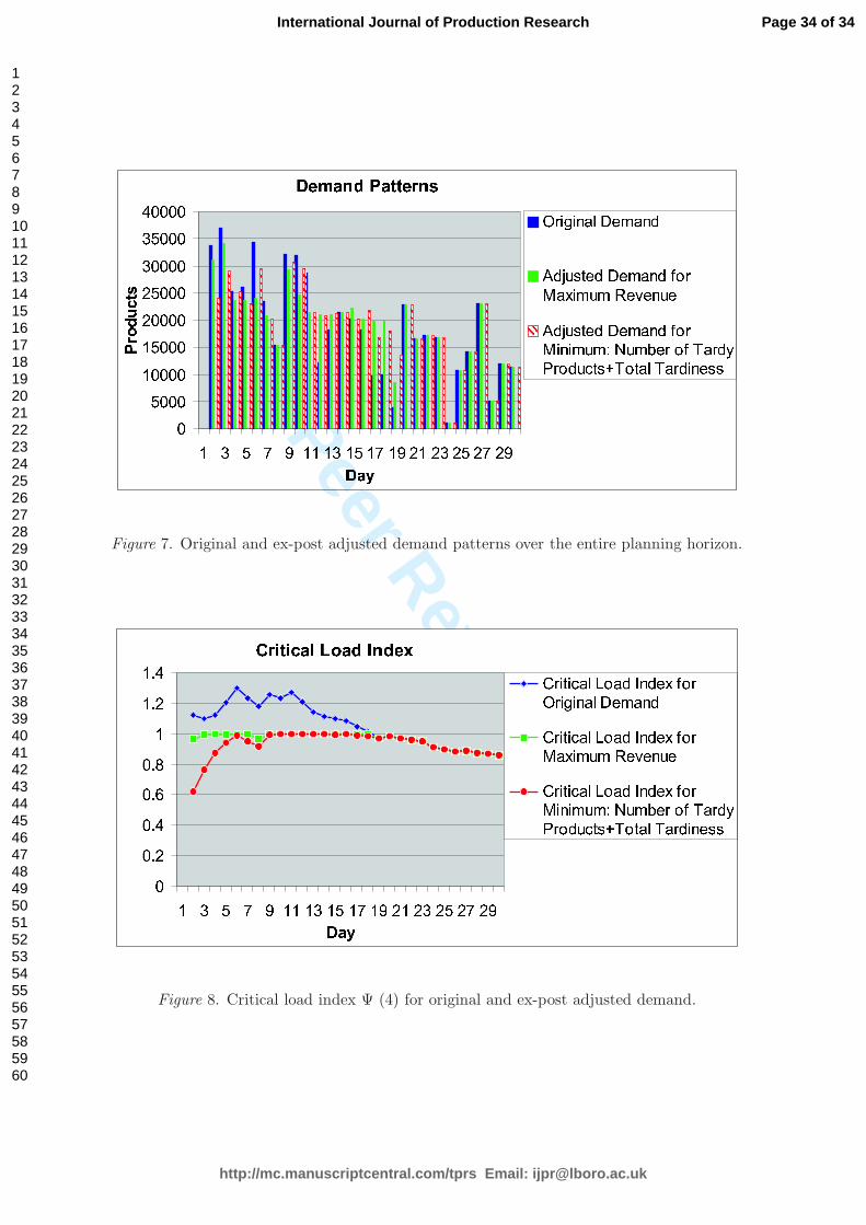
The original demand pattern and the ex-post adjusted demand patterns for various ob-

jective functions are compared in Fig. 7. The corresponding critical load index Ψ (4) for the

original and the ex-post adjusted demands is shown in Fig. 8, where Ψ(d) ≤ 1, ∀d ∈ T for

the adjusted demand patterns. Fig. 8 demonstrates that the primary objective of minimizing

20

Page 20 of 34

http://mc.manuscriptcentral.com/tprs Email: [email protected]

International Journal of Production Research

123456789101112131415161718192021222324252627282930313233343536373839404142434445464748495051525354555657585960

For Peer Review O

nlyFigure 6. Ex-post adjusted demand patterns with maximum revenue for different service

levels.

the number of delayed products leads to smaller values of Ψ at the beginning of the horizon

for the adjusted demand, where Ψ > 1 for the original demand. In contrast, the objective of

maximizing total revenue leads to more smoothed utilization of the capacity over the horizon.

Figure 7. Original and ex-post adjusted demand patterns over the entire planning horizon.

Figure 8. Critical load index Ψ (4) for original and ex-post adjusted demand.

The solution values shown in Table 4 indicate that the reduction of the total number of

delayed products (Psum = 39795 vs. Psum = 47690 or Psum = 47815, respectively for the

secondary criterion Qsum or Qmax) leads to a higher revenue (Rsum = 535612 or Rsum =

535549 vs. Rsum = 533313 or Rsum = 530578, respectively for the secondary criterion Qsum

or Qmax), though the number of delayed orders is greater (Osum = 10 or Osum = 18 vs.

Osum = 8, respectively for the secondary criterion Qsum or Qmax), and by this the service

level γ is lower. The results indicate that the minimum number of delayed orders can be

achieved by delaying a few, large orders.

The adjusted demand patterns and the corresponding solution values demonstrate that

for a higher service level, more demand is reallocated to later periods, however the number of

delayed orders is reduced, which indicates that mainly large customer orders are selected for

reallocation to achieve the required service level. The results indicate that the higher service

level required, the smaller total number of delayed orders and the greater total number of

delayed products.

Table 4 also compares the weighted-sum and the lexicographic approach for the bi-objective

problem formulations. The table indicates that CPU times are much smaller for the lexico-

graphic approach. In the example presented in Table 4, the optimal value Osum = 8 or

Psum = 39795 for the primary objective function is identical for the two approaches, whereas

the secondary objective functions Qsum, Qmax are slightly greater for the lexicographic ap-

proach, since the optimal value of the primary objective can be achieved for alternative subsets

of delayed orders.

Finally, the following simple example illustrates an attempt to find a subset of non-

dominated solutions to the bi-objective due date setting problem for the entire planning hori-

zon. In the example f1 = Osum, f2 ∈ {Qsum, Qmax}, and the non-dominated solutions are de-

21

Page 21 of 34

http://mc.manuscriptcentral.com/tprs Email: [email protected]

International Journal of Production Research

123456789101112131415161718192021222324252627282930313233343536373839404142434445464748495051525354555657585960

For Peer Review O

nly

termined by parameterizing the weighted-sum program DDS on λ1 = 0.1, 0.2, 0.3, 0.4, 0.5, 0.6,

0.7, 0.8, 0.9 with λ2 = 1 − λ1.

For the objective function λ1Osum +(1−λ1)Qsum, only two non-dominated solutions were

found: Osum = 11, Qsum = 68 for λ1 = 0.1, 0.2, 0.3, 0.4, 0.5 and Osum = 8, Qsum = 71 for

λ1 = 0.6, 0.7, 0.8, 0.9, and only one solution was found for the objective function λ1Osum +

(1 − λ1)Qmax: Osum = 11, Qmax = 15 for all λ1 = 0.1, 0.2, 0.3, 0.4, 0.5, 0.6, 0.7, 0.8, 0.9.

Let us note, however, that the non-dominated solution set of the bi-objective due date set-

ting problem cannot be fully determined even by complete parameterizing on λ the weighted-

sum program DDS. To compute unsupported non-dominated solutions, some upper bounds

on the objective function values should be added to DDS, e.g. Alves and Climaco (2007).

7. Conclusion

The simple integer programming approach proposed in this paper is capable of setting due

dates in make-to-order environment, either in a batch mode, where customer orders are col-

lected over a specified time interval or in a real-time mode, where a commitment due date is

determined at the time of the customer order arrival. While the real-time mode is preferable

by the customer, the batch mode offers the manufacturer more demand-pattern information,

and the longer is the batching interval, the larger is the set of orders to optimize over. On

the other hand, the computational effort required in real-time mode, where only a few newly-

arrived orders are considered at a time is much less than that for the batch mode, where a set

of customer orders should be considered simultaneously. The proposed approach is determin-

istic in nature, however, its usage on the rolling horizon basis, allows for reactive decisions to

be made in response to various disruptions in a supply chain.

Limited computational experiments indicate that the weighted-sum approach may outper-

form the lexicographic approach if multiple optima exist with the same value of the primary

objective function, i.e., if alternative minimal subsets of delayed and rejected orders exist. In

this case, a smaller total or maximum delay may sometimes be achieved for the weighted-sum

approach. The lexicographic approach, however, requires the much smaller CPU time to find

the optimal solutions and hence seems to be more suitable for setting optimal due date for

each newly-arrived order in a real-time mode. In particular, when the customer expects an

immediate confirmation of the order acceptance (or rejection), where otherwise the potential

customer can be lost, e.g. in e-Business. The small computational effort required for the

proposed model and its quite general setting may prove its usefulness as a simple decision

support tool for a rough-cut capacity allocation in the other make-to-order environments,

22

Page 22 of 34

http://mc.manuscriptcentral.com/tprs Email: [email protected]

International Journal of Production Research

123456789101112131415161718192021222324252627282930313233343536373839404142434445464748495051525354555657585960

For Peer Review O

nly

different from the flexible flowshop considered in this paper.

The capacity evaluation at the customer enquiry stage is a critical issue in make to order

manufacturing and has a large impact on customer service and reliability of order fulfillment.

The introduced critical load index can be applied to quickly identify the system bottleneck

and the overloaded periods. In contrast to the order acceptance models based on scheduling

with due date objectives, where the computational effort required can be prohibitive.

The model proposed directly links customer orders with available capacity, whereas the

other resources are assumed to be non-binding, in particular material availability is not con-

sidered. The integer programming formulations can be enhanced to account also for a limited

material availability. Then, additional material availability constraints should be added to

the model. However, an important issue that remains for further investigation is how to best

coordinate the due date setting decisions and the subsequent order scheduling subject to ma-

terial availability to arrive at a feasible schedule with all accepted orders completed by the

committed due dates.

In practice, a customer request for quotation may consist of the required quantities of

several product types and the requested delivery dates. Then, a typical response to such a

customer request should contain the quantity to be fulfilled, the date of delivery and the price

based on revenue management principles which may involve penalties associated to deviations

from the customer requested quantities and dates. The approach proposed in this paper can

be enhanced to handle multiple product orders. The pricing decisions, however, should be

based on both tactical factors such as estimated costs, as well as strategic factors, such as

the value of a long-term relationship with a customer and the rejection costs. Despite its

importance, the price optimization issue in due date setting is underexposed in the literature.

Acknowledgments

The author is grateful to two anonymous reviewers for reading the manuscript carefully and

providing constructive comments which helped to improve this paper. This work has been

partially supported by research grant of MNiSzW (N 519 03432/4143) and by AGH.

References

Akkan, C. 1997. Finite-capacity scheduling-based planning for revenue-based capacity man-

agament. European Journal of Operational Research, 100, 170–179.

Alves, M.J., Climaco, J., 2007. A review of interactive methods for multiobjective integer and

mixed-integer programming. European Journal of Operational Research, 180, 99-115.

23

Page 23 of 34

http://mc.manuscriptcentral.com/tprs Email: [email protected]

International Journal of Production Research

123456789101112131415161718192021222324252627282930313233343536373839404142434445464748495051525354555657585960

For Peer Review O

nly

Bertrand, J.W.M., van Ooijen, H.P.G., 2000. Customer order lead times for production based

on lead times and tardiness costs. International Journal of Production Economics, 64,

257–265.

Chen, C.-Y., Zhao, Z.-Y., Ball, M.O., 2001. Quantity and due date quoting available to

promise. Information Systems Frontiers, 3(4), 477–488.

Corti, D., Pozzetti, A., Zorzini, M., 2006. A capacity-driven approach to establish reliable

due dates in MTO environment. International Journal of Production Economics, 104,

536–554.

Ebben, M.J.R., Hans, E.W., Olde Weghuis, F.M., 2005. Workload based acceptance in job

shop environments, OR Spectrum, 27, 107–122.

Geunes, J., Romeijn, H.E., Taaffe, K., 2006. Requirements planning with pricing and order

selection flexibility. Operations Research, 54(2), 394–401.

Harris, F.H., Pinder, J.P., 1995. Revenue management approach to demand management and

order booking in assemble-to-order manufacturing. Journal of Operations Management,

13(4), 299–309.

Hegedus, M.G., Hopp, W.J., 2001. Due date setting with supply constraints in systems using

MRP. Computers & Industrial Engineering, 39, 293–305.

Lewis, H.F., Slotnick, S.A.,2002. Multi-period job selection: planning work loads to maxi-

mize profit. Computers & Operations Research, 29, 1081–1098.

Sawik, T., 2007a. A lexicographic approach to bi-objective scheduling of single-period orders

in make-to-order manufacturing. European Journal of Operational Research, 180(3),

1060-1075.

Sawik, T., 2007b. Multi-objective master production scheduling in make-to-order manufac-

turing, International Journal of Production Research, 45(12), 2629-2653.

Slotnick, S.A., Morton, T.E., 1996. Selecting jobs for a heavily loaded shop with lateness

penalties. Computers & Operations Research, 23(2), 131–140.

Smutnicki, C., 2007. Scheduling with high variety of customized compound products. Deci-

sion Making in Manufacturing and Services, 1(1-2), 91–110.

Steuer, R.E., 1986. Multiple Criteria Optimization: Theory, Computation and Application.

Wiley, New York.

Wester, F.A.W., Wijngaard, J.,Zijm, W.H.M., 1992. Order acceptance strategies in a

production-to-order environment with setup times and due dates. International Journal

of Production Research, 30(4), 1313–1326.

24

Page 24 of 34

http://mc.manuscriptcentral.com/tprs Email: [email protected]

International Journal of Production Research

123456789101112131415161718192021222324252627282930313233343536373839404142434445464748495051525354555657585960

For Peer Review O

nly

Zorzini, M., Corti, D., Pozzetti, A., 2008. Due date (DD) quotation and capacity planning

in make-to-order companies: Results from an empirical analysis. International Journal

of Production Economics, 112, 919–933.

25

Page 25 of 34

http://mc.manuscriptcentral.com/tprs Email: [email protected]

International Journal of Production Research

123456789101112131415161718192021222324252627282930313233343536373839404142434445464748495051525354555657585960

For Peer Review O

nlyDue Date Setting

DDS

Scheduling Customer Orders

SCO

?

?

?

-

Planning Horizon: hBatching Interval: t1 − σ ≤ t < t1

New Orders: {j ∈ J : aj , dj , sj}

Remaining Orders: {j ∈ J : aj , dj , sj}

t1 = t1 + σ

aj = max{t1, dj − Emax}Due Dates:

dj , if j ∈ J : xj = 1∑

t∈T :t>djtyjt, if j ∈ J : xj = 0, yjh∗ = 0

dj , if j ∈ J

{j : zjt = 1, t ≥ t1 + σ}

Maximum Earliness: Emax

Order Assignment: {j : zjt = 1, t1 ≤ t < t1 + h}

Figure 1. Due date setting and scheduling of customer orders over a rolling planning horizon.

Order Acceptance

OA

Due Date Setting

DD

?

?

?

New Orders: {j ∈ J : aj , dj , sj}

Remaining Orders: {j ∈ J : aj, dj , sj}-

Accepted Orders: {j ∈ J : xj = 1}

Delayed or Rejected Orders: {j ∈ J : xj = 0}

Due Dates:

dj , if j ∈ J : xj = 1∑

t∈T :t>djtyjt, if j ∈ J : xj = 0, yjh∗ = 0

dj , if j ∈ J

Figure 2. A two-level order acceptance and due date setting.

Page 26 of 34

http://mc.manuscriptcentral.com/tprs Email: [email protected]

International Journal of Production Research

123456789101112131415161718192021222324252627282930313233343536373839404142434445464748495051525354555657585960

For Peer Review O

nlyTable 1. Notation

Indices

i = processing stage, i ∈ I

j = customer order, j ∈ J⋃

J

t = planning period, t ∈ T

Input Parameters

aj , sj = ready date, size of order j

cit = processing time available in period t on each machine in stage i

Ci(t, d) = cumulative capacity available in stage i in periods t through d

dj , (dj) = customer requested (manufacturer quoted) due date for order j ∈

J, (j ∈ J)

h = planning horizon

mi = number of identical, parallel machines in stage i

pij = processing time in stage i of each product in order j

qij = pijsj - total processing time required to complete order j in stage i

σ = length of batching interval

J = set of newly-arrived customer orders collected over a batching interval

J = set of previously-accepted customer orders, remaining for processing

Decision variables

xj = 1, if order j is accepted with customer requested due date; xj = 0 if

order j needs to be delayed or rejected (order acceptance variable)

yjt = 1, if order j is assigned delayed due date t, (dj < t < h∗) or is rejected

(t = h∗); otherwise yjt = 0 (due date setting variable)

zjt = 1, if customer order j is assigned to planning period t; otherwise

zjt = 0 (order assignment variable)

wjt ∈ [0, 1] = fraction of multi-period order j assigned to period t (multi-period

order allocation variable)

Emax = maximum earliness

Osum, Psum = total number of delayed orders, delayed products, respectively

Qmax, Qsum = maximum delay, total delay, respectively

Rsum = total revenue

Page 27 of 34

http://mc.manuscriptcentral.com/tprs Email: [email protected]

International Journal of Production Research

123456789101112131415161718192021222324252627282930313233343536373839404142434445464748495051525354555657585960

For Peer Review O

nly

Table 2. Computational results: model DDS

Batching Interval Var. Bin. Cons. Solution values CPU†

/Planning Interval

Objective function: min(10Osum + Qsum)

t < 1/[1, 20] 7565 7565 1541 Osum = 8, Qsum = 71, (Psum = 47690, Qmax = 17, Rsum = 405556) 19.8

[1, 5]/[6, 25] 250 250 109 Osum = 0, Qsum = 0, (Psum = 0, Qmax = 0, Rsum = 369885) 0.02

[6, 10]/[11, 30] 285 285 158 Osum = 2, Qsum = 2, (Psum = 3675, Qmax = 1, Rsum = 324116) 0.03

Objective function: min(10Osum + Qmax)

t < 1/[1, 20] 7566 7565 8480 Osum = 8, Qmax = 14, (Psum = 48265, Qsum = 94, Rsum = 403806) 257

[1, 5]/[6, 25] 251 250 304 Osum = 0, Qmax = 0, (Psum = 0, Qsum = 0, Rsum = 378270) 0.02

[6, 10]/[11, 30] 286 285 369 Osum = 2, Qmax = 1, (Psum = 4225, Qsum = 2, Rsum = 332850) 0.02

Objective function: min(Psum + Qsum)

t < 1/[1, 20] 7565 7565 1541 Psum = 39795, Qsum = 78, (Osum = 10, Qmax = 17, Rsum = 407902) 148

[1, 5]/[6, 25] 250 250 112 Psum = 0, Qsum = 0, (Osum = 0, Qmax = 0, Rsum = 375520) 0.01

[6, 10]/[11, 30] 285 285 158 Psum = 2000, Qsum = 4, (Osum = 4, Qmax = 1, Rsum = 321185) 0.1

Objective function: min(Psum + Qmax)

t < 1/[1, 20] 7566 7565 8480 Psum = 39795, Qmax = 11, (Osum = 93, Qsum = 922, Rsum = 408450) 347

[1, 5]/[6, 25] 251 250 301 Psum = 0, Qmax = 0, (Osum = 0, Qsum = 0, Rsum = 373610) 0.02

[6, 10]/[11, 30] 286 285 369 Psum = 2000, Qmax = 1, (Osum = 4, Qsum = 4, Rsum = 321325) 0.04

Objective function: max Rsum

t < 1/[1, 20] 7565 7565 1541 Rsum = 409426, (Osum = 47, Psum = 39815, Qsum = 492, Qmax = 16) 225

[1, 5]/[6, 25] 250 250 111 Rsum = 370400, (Osum = 0, Psum = 0, Qsum = 0, Qmax = 0) 0

[6, 10]/[11, 30] 285 285 158 Rsum = 315850, (Osum = 5, Psum = 2000, Qsum = 5, Qmax = 1) 0.03† CPU seconds for proving optimality on a PC Pentium IV, 2.4GHz, RAM 512MB /CPLEX v.9

Osum =∑

j∈J(1 − xj) - total number of delayed orders

Psum =∑

j∈Jsj(1 − xj) - total number of delayed products

Qsum =∑

j∈J,t∈T :t>dj(t − dj)yjt - total delay

Qmax = maxj∈J,t∈T :t>dj(t − dj)yjt - maximum delay

Rsum =∑

j∈Jrjsjxj +

∑

j∈J,t∈T :t>djrjtsjyjt - total revenue (rj = 1 and rjt = 0.80 − 0.02(t − dj); t > dj , j ∈ J)

Page 28 of 34

http://mc.manuscriptcentral.com/tprs Email: [email protected]

International Journal of Production Research

123456789101112131415161718192021222324252627282930313233343536373839404142434445464748495051525354555657585960

For Peer Review O

nlyTable 3. Computational results: model SCO1

Planning Interval Var. Bin. Cons. Solution value CPU†

Objective function of DDS: min(10Osum + Qsum)

[1, 20] 5905 5904 6007 Emax = 2 6.3

[6, 25] 3113 3112 3211 Emax = 0 0.17

[11, 30] 3120 3119 3211 Emax = 0 0.14

Objective function of DDS: min(10Osum + Qmax)

[1, 20] 5957 5958 6059 Emax = 2 13

[6, 25] 3094 3093 3180 Emax = 0 0.15

[11, 30] 3174 3173 3265 Emax = 0 0.16

Objective function of DDS: min(Psum + Qsum)

[1, 20] 5888 5887 5990 Emax = 2 109

[6, 25] 2742 2741 2832 Emax = 0 0.16

[11, 30] 3023 3022 3115 Emax = 0 0.13

Objective function of DDS: min(Psum + Qmax)

[1, 20] 6099 6098 6201 Emax = 2 5.4

[6, 25] 3802 3801 3893 Emax = 0 0.38

[11, 30] 2976 2975 3068 Emax = 0 0.13

Objective function of DDS: max Rsum

[1, 20] 6095 6094 6196 Emax = 2 21

[6, 25] 3096 3095 3176 Emax = 0 0.14

[11, 30] 2924 2923 3015 Emax = 0 0.15† CPU seconds for proving optimality on a PC Pentium IV, 2.4GHz, RAM 512MB /CPLEX v.9

Emax - maximum earliness

Page 29 of 34

http://mc.manuscriptcentral.com/tprs Email: [email protected]

International Journal of Production Research

123456789101112131415161718192021222324252627282930313233343536373839404142434445464748495051525354555657585960

For Peer Review O

nly

Figure 3. Demand patterns and production over a rolling planning horizon for minimum:

10 x delayed orders + total delay.

Page 30 of 34

http://mc.manuscriptcentral.com/tprs Email: [email protected]

International Journal of Production Research

123456789101112131415161718192021222324252627282930313233343536373839404142434445464748495051525354555657585960

For Peer Review O

nly

Figure 4. Demand patterns and production over a rolling planning horizon for minimum:

delayed products + total delay.

Page 31 of 34

http://mc.manuscriptcentral.com/tprs Email: [email protected]

International Journal of Production Research

123456789101112131415161718192021222324252627282930313233343536373839404142434445464748495051525354555657585960

For Peer Review O

nly

Figure 5. Demand patterns and production over a rolling planning horizon for maximum

revenue.

Page 32 of 34

http://mc.manuscriptcentral.com/tprs Email: [email protected]

International Journal of Production Research

123456789101112131415161718192021222324252627282930313233343536373839404142434445464748495051525354555657585960

For Peer Review O

nlyTable 4. Computational results: ex-post solutions

Objective function Var. Bin. Cons. Solution values CPU†

Weighted-sum approach: model DDS

10Osum + Qsum 14913 14913 3019 Osum = 8, Qsum = 71, (Psum = 47690, Qmax = 17, Rsum = 533313) 71

10Osum + Qmax 14914 14913 17141 Osum = 8, Qmax = 14, (Psum = 47815, Qsum = 98, Rsum = 530578) 2473

Lexicographic approach - models OA and DD

Osum 808 808 48 Osum = 8 0.25

Qsum 112 112 294 Qsum = 73 0.11

Qmax 113 112 406 Qmax = 15 0.15

Weighted-sum approach: model DDS

Psum + Qsum 14913 14913 3019 Psum = 39795, Qsum = 78, (Osum = 10, Qmax = 17, Rsum = 535612) 690

Psum + Qmax 14914 14913 17141 Psum = 39795, Qmax = 12, (Osum = 18, Qsum = 178, Rsum = 535549) 2233

Lexicographic approach - models OA and DD

Psum 808 808 85 Psum = 39795 12

Qsum 965 965 374 Qsum = 88 0.24

Qmax 966 965 1339 Qmax = 12 5

Rsum 14913 14913 3019 Rsum = 537132, (Osum = 52, Psum = 39805, Qsum = 456, Qmax = 17) 432

Rsum|γ = 90% 14913 14913 3020 Rsum = 537108, (Osum = 42, Psum = 39805, Qsum = 422, Qmax = 16) 189

Rsum|γ = 95% 14913 14913 3020 Rsum = 537106, (Osum = 40, Psum = 39805, Qsum = 343, Qmax = 16) 388

Rsum|γ = 99% 14913 14913 3020 Rsum = 533820, (Osum = 8, Psum = 44235, Qsum = 76, Qmax = 15) 146† CPU seconds for proving optimality on a PC Pentium IV, 2.4GHz, RAM 512MB /CPLEX v.9

Osum =∑

j∈J(1 − xj) - total number of delayed orders

Psum =∑

j∈Jsj(1 − xj) - total number of delayed products

Qsum =∑

j∈J,t∈T :t>dj(t − dj)yjt - total delay

Qmax = maxj∈J,t∈T :t>dj(t − dj)yjt - maximum delay

Rsum =∑

j∈Jrjsjxj +

∑

j∈J,t∈T :t>djrjtsjyjt - total revenue (rj = 1 and rjt = 0.80 − 0.02(t − dj); t > dj , j ∈ J)

Figure 6. Ex-post adjusted demand patterns with maximum revenue for different service

levels.

Page 33 of 34

http://mc.manuscriptcentral.com/tprs Email: [email protected]

International Journal of Production Research

123456789101112131415161718192021222324252627282930313233343536373839404142434445464748495051525354555657585960

For Peer Review O

nly

Figure 7. Original and ex-post adjusted demand patterns over the entire planning horizon.

Figure 8. Critical load index Ψ (4) for original and ex-post adjusted demand.

Page 34 of 34

http://mc.manuscriptcentral.com/tprs Email: [email protected]

International Journal of Production Research

123456789101112131415161718192021222324252627282930313233343536373839404142434445464748495051525354555657585960