Multi-Objective Compared to Single-Objective Optimization ...

DGMK/ÖGEW-Frühjahrstagung 2007, Fachbereich Aufsuchung und Gewinnung, Celle

DGMK-Tagungsbericht 2007-1, ISBN 978-3-936418-65-1

Multi-Objective Compared to Single-Objective Optimization with Application to Model Validation and Uncertainty Quantification R. Schulze-Riegert*, M. Krosche*, K. Stekolschikov*, A. Fahimuddin**, *Scandpower Petroleum Technology GmbH, Hamburg, ** TU Braunschweig

Abstract

History Matching in Reservoir Simulation, well location and production optimization etc. is generally a multi-objective optimization problem. The problem statement of history matching for a realistic field case includes many field and well measurements in time and type, e.g. pressure measurements, fluid rates, events such as water and gas break-throughs, etc. Uncertainty parameters modified as part of the history matching process have varying impact on the improvement of the match criteria. Competing match criteria often reduce the likelihood of finding an acceptable history match. It is an engineering challenge in manual history matching processes to identify competing objectives and to implement the changes required in the simulation model. In production optimization or scenario optimization the focus on one key optimization criterion such as NPV limits the identification of alternatives and potential opportunities, since multiple objectives are summarized in a predefined global objective formulation. Previous works primarily focus on a specific optimization method. Few works actually concentrate on the objective formulation and multi-objective optimization schemes have not yet been applied to reservoir simulations. This paper presents a multi-objective optimization approach applicable to reservoir simulation. It addresses the problem of multi-objective criteria in a history matching study and presents analysis techniques identifying competing match criteria. A Pareto-Optimizer is discussed and the implementation of that multi-objective optimization scheme is applied to a case study. Results are compared to a single-objective optimization method.

Introduction

In recent years there has been more and more attention given to workflows for uncertainty assessment in reservoir management. Structured approaches exist for assessing the impacts of uncertainty on investment decision-making in the oil and gas industry1. These approaches mostly rely on simplified component models for each decision domain such as G&G models, production scenarios, drilling models, processing facilities, economics and related costs. Because of its complexity, the integration of dynamical modelling is only gradually entering this domain of decision-making processes. It is generally accepted that any model reliably predicting future quantities should be able to reproduce known history data. This requires a model validation process2 (History Matching) which is traditionally cumbersome and time consuming. The consistent inclusion of production data calls for computation-intensive processing. This requires new approaches in the application of experimental design and optimization methods which is supported by the use of high-performance computing facilities3,4. One crucial change in the mind set within reservoir engineering is the accepted importance of including multiple realizations of dynamical reservoir models into the forward modelling process to account for uncertainties in the prediction phase5,6. Although several studies on deriving multiple solutions to a History Matching problem6-9 have been published recently there are nevertheless no structured workflows or optimization

methods applicable to reservoir simulation which address the problem of multi-objective optimization MOO10-13. Recent analysis of the TDRM6 workflow within the context of History Matching has identified single-objective optimization techniques as one weakness vis-à-vis manual history matching7. This work extends the application of MOOs which are already applied in other industry areas and focuses on an implementation of a multi-objective optimization technique with applications in reservoir simulation. With an extension to a previous publication16, the Multi-objective optimization scheme is compared to a Single-objective optimization scheme. Multi-objective optimization criteria in reservoir simulation are not just addressing the problem statement of History Matching. Other examples include production optimization, portfolio optimization, etc. The methodology used in this work is described in the next chapter. A practical comparison to a single-objective optimization technique is given in the last chapter. Readers interested only in principal capabilities of the multi-objective optimization technique and results should refer to the implementation chapter and the application to History Matching.

Methodology

This section describes the principal methodology and workflow of a multi-objective optimization technique. The choice of optimization methods supporting the process of history matching in reservoir engineering depends to a considerable degree on the problem statement. Irrespective of the available optimization technique, good understanding of reservoir data, existing uncertainties, accuracy of production data, etc., is a prerequisite for the formulation of the optimization problem. Objective Function Definition History Matching is in general a constrained non-linear optimization problem2. The difference between the observed values and calculated values defines the quality of the history match and is described by the objective function f. Most often a quadratic definition of the objective function is used, i.e.,

[ ]∑∑∑= = =

−=i j kn

i

n

j

n

k

obscalc kjiykjiykjiXf1 1 1

2),,(),,(),,()( ω (1)

where calcobs yy , denote the observation and simulation values, respectively, ),,( kjiϖ

captures parameter weighting coefficients. The indices ),,( kji refer to all wells, measurement values and time steps;

in ,jn ,

kn are the corresponding maximum values of

),,( kji and X describes the optimal vector. For a typical history matching problem the objective function is an implicit function of the optimal vector. Thus, a general history matching problem can be posted as an inequality constrained non-linear optimization problem having the following form:

miXg

EXXf

i

n

,,2,10)(

)(min

K=≥

∈ (2)

The optimal vector X, the objective function f(X) and the inequality constrained vector g(X) are different for each history matching problem. The standard approach followed in solving the above non-linear optimization problem is to use iterative deterministic or stochastic techniques. Recently Evolutionary Algorithms, e.g. Genetic Algorithms13 or Evolution Strategies14,15 have been employed to handle global optimization issues. Multi-objective Optimization Optimization problems involving multiple, conflicting objectives are often addressed by aggregating the objectives into a scalar function and solving the resulting single-objective optimization problem. In contrast, our focus is on finding a set of optimal trade-offs, the so-called Pareto-optimal set. In the following, we formalize this established concept10-13. A multi-objective search space is partially ordered in the sense that two arbitrary solutions are related to each other in two possible ways: either one dominates the other or neither dominates.

2

Definition 1: Let us consider, without loss of generality, a multi-objective minimization problem with m decision variables (uncertainty parameters) and n objectives:

( )

( )

( ) Yyyy

Xxxx

xfxfxfy

n

m

n

∈=

∈=

==

,,

,,where

)(,),()(Minimize

1

1

1

K

K

K

(3)

x is called a decision vector, X parameter space, y objective vector and Y objective space. A decision vector Xa ∈ is said to dominate a decision vector Xb ∈ (also written ba f ) if and only if

{ }

{ } )()(:,,1

)()(:,,1

bfafnj

bfafni

jj

ii

<∈∃

∧≤∈∀

K

K (4)

Based on the above relation, we can define non-dominated and Pareto-optimal solutions: Definition 2: Let Xa ∈ be an arbitrary decision vector: The decision vector a is said to be non-dominated regarding a set XX ⊆' if and only if there is no vector in 'X which dominates a; formally

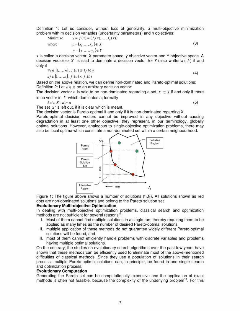
aaXa f':''∈∃/ (5) The set 'X is left out, if it is clear which is meant. The decision vector is Pareto-optimal if and only if it is non-dominated regarding X. Pareto-optimal decision vectors cannot be improved in any objective without causing degradation in at least one other objective; they represent, in our terminology, globally optimal solutions. However, analogous to single-objective optimization problems, there may also be local optima which constitute a non-dominated set within a certain neighbourhood. �

2

�1

FeasibleRegion

InfeasibleRegion

min

min

Pareto Front

Pareto Solution

Set

Figure 1: The figure above shows a number of solutions (f1,f2). All solutions shown as red dots are non-dominated solutions and belong to the Pareto solution set. Evolutionary Multi-objective Optimization In dealing with multi-objective optimization problems, classical search and optimization methods are not sufficient for several reasons11:

I. Most of them cannot find multiple solutions in a single run, thereby requiring them to be applied as many times as the number of desired Pareto-optimal solutions,

II. multiple application of these methods do not guarantee widely different Pareto-optimal solutions will be found, and

III. most of them cannot efficiently handle problems with discrete variables and problems having multiple optimal solutions.

On the contrary, the studies on evolutionary search algorithms over the past few years have shown that these methods can be efficiently used to eliminate most of the above-mentioned difficulties of classical methods. Since they use a population of solutions in their search process, multiple Pareto-optimal solutions can, in principle, be found in one single search and optimization process. Evolutionary Computation Generating the Pareto set can be computationally expensive and the application of exact methods is often not feasible, because the complexity of the underlying problem17. For this

3

reason, a number of stochastic search strategies such as Evolutionary Algorithms, taboo search and simulated annealing, etc., have been further developed to address multi-objective optimization capabilities: They usually do not guarantee that optimal trade-offs will be identified, but try to find a good approximation to the Pareto Front. In this work we concentrate on Evolutionary Algorithms. Broadly speaking, an Evolutionary Algorithm is characterized by three features:

• A set of solution candidates is maintained, • a mating selection process is performed on this set, and • several solutions may be combined in terms of recombination to generate new

solutions. Using biological evolution in nature as an analogy, the solution candidates are called individuals and the set of solution candidates is called the population. Each individual represents a possible solution to the optimization problem. Algorithm Design Issues Two major design requirements must be addressed when an Evolutionary Algorithm is applied to multi-objective optimization:

• How to accomplish fitness assignment and selection, respectively, in order to guide the search towards the Pareto-optimal set, cf. left figure below.

• How to maintain a diverse population in order to prevent premature convergence and achieve a well distributed trade-off front, cf. right figure below. ��

����

��

Figure 2: Algorithm design issues; best approximation of the Pareto front, left figure, and diversity preservation, right plot. Often, different approaches are classified with regard to the first issue, where one can distinguish between criterion selection, aggregation selection, and Pareto selection18. Pareto selection makes direct use of the dominance relation from Definition 1; Goldberg was the first to suggest a Pareto-based fitness assignment strategy13. For an overview of different multi-objective optimization methods based on evolutionary algorithms, we refer the reader to the work of Coello et al.10 In this work, we focus on one Pareto-based technique called the Strength Pareto Evolutionary Algorithm (SPEA)17.

Implementation

The Strength Pareto Evolutionary Algorithm (SPEA) is a recently developed technique for finding or approximating the Pareto set for multi-objective optimization problems. In different performance tests, SPEA compared favourably with other MOEAs and has therefore served as a point of reference in various recent investigations. Furthermore, it has been used in different applications. In this work, the implementation and application of an improved version, SPEA2, is first explained and subsequently applied to a very simple two-dimensional problem in order to illustrate the concepts. Compared to traditional Evolutionary Algorithms, the Pareto Optimizer (SPEA) uses a regular population and an archive (external set). Starting with an initial population and an empty archive, the following steps are performed in each iteration. First, all non-dominated members of a population are selected and copied to the archive; any dominated individuals or duplicates (regarding the objective values) are removed from the archive during this update operation. If the size of the updated archive exceeds a predefined limit, further archive members are deleted by a clustering technique which preserves the characteristics of the non-dominated front. Afterwards, fitness values are assigned to both archive and population members:

4

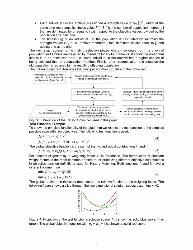
• Each individual i in the archive is assigned a strength value [ ]1,0)( ∈iS , which at the same time represents its fitness value F(i). S(i) is the number of population members j that are dominated by or equal to i with respect to the objective values, divided by the population size plus one.

• The fitness F(j) of an individual j in the population is calculated by summing the strength values S(i) of all archive members i that dominate or are equal to j, and adding one at the end.

The next step represents the mating selection phase where individuals from the union of population and archive are selected by means of binary tournaments. It should be noted that fitness is to be minimized here, i.e., each individual in the archive has a higher chance of being selected than any population member. Finally, after recombination and mutation the old population is replaced by the resulting offspring population. The following diagram describes the principal workflow structure of the optimizer:

Initialization: Genrate an initialpopulation P0 and create theempty archive A0=0. Set t=0

Fitness assignment: Calculate fitnessvalues of individuals in Pt and At

Environmental selection: Copy allnondominated individuals in Pt and At to

At+1.

Termination: Check stop criteria.If criteria is satisfied A* is the set ofdecision vectors represented by the

nondominated individuals in At+1

Mating selection: Perform binarytournament selection with replacementon At+1 in order to fill the mating pool.

Variation: Apply genetic operators to themating pool and set Pt+1 to the resulting

population. t->t+1

OutputA* (nondominated set)

Figure 3: Workflow of the Pareto Optimizer used in this paper. Test Function Example To show the principle functionality of the algorithm we restrict the test function to the simplest possible case with two objectives. The following test function is used:

2

2

2

1212

2

2

2

1211

)0.5()0.5(),(

),(

−+−=

+=

xxxxf

xxxxf (6)

The global objective function is the sum of the two individual contributions f1 and f2. ),(),(),( 2122211121 xxfxxfxxf ωω += (7)

For reasons of generality, a weighting factor ω is introduced. The introduction of constant weight factors is the most common procedure for prioritizing different objective contributions in objective function definitions used for History Matching. Both functions f1 and f2 have a different optimum, i.e.

)5,5(),(min

)0,0(),(min

2212

1211

fxxf

fxxf

=

= (8)

The global optimum in this case depends on the relative fraction of the weighing factor. The following figure shows a slice through the two dimensional solution space, assuming x2=0.

020406080

100120140160

-5 0 5 10

Figure 4: Projection of the test function’s solution space. f1 is shown as solid blue curve, f2 as green. The global objective function with 121 == ωω is shown as solid red curve.

5

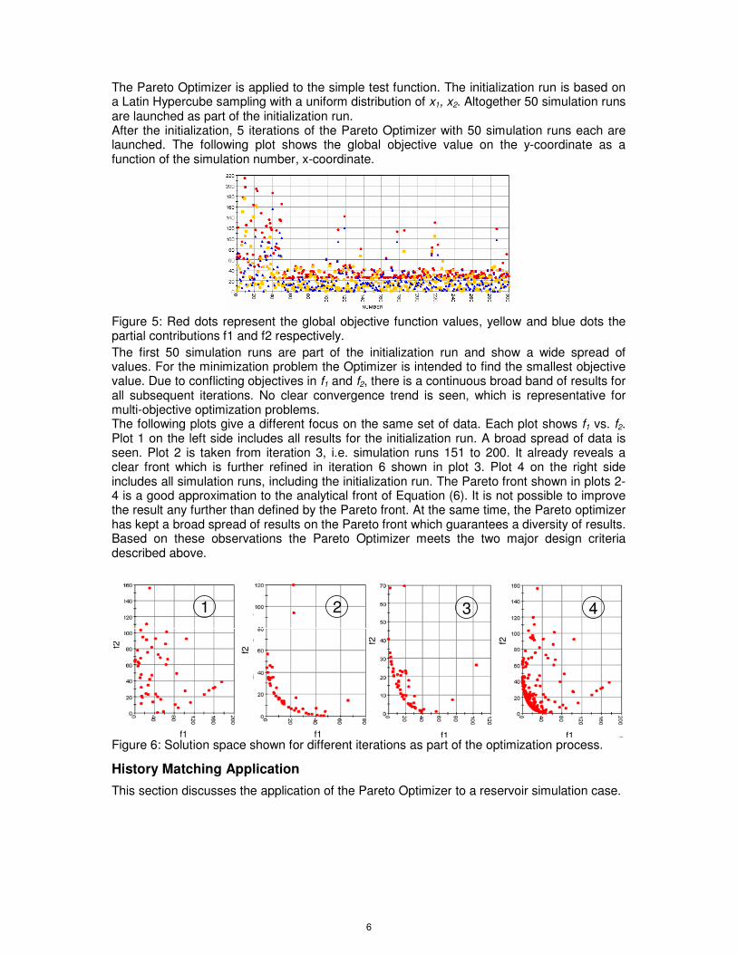
The Pareto Optimizer is applied to the simple test function. The initialization run is based on a Latin Hypercube sampling with a uniform distribution of x1, x2. Altogether 50 simulation runs are launched as part of the initialization run. After the initialization, 5 iterations of the Pareto Optimizer with 50 simulation runs each are launched. The following plot shows the global objective value on the y-coordinate as a function of the simulation number, x-coordinate.

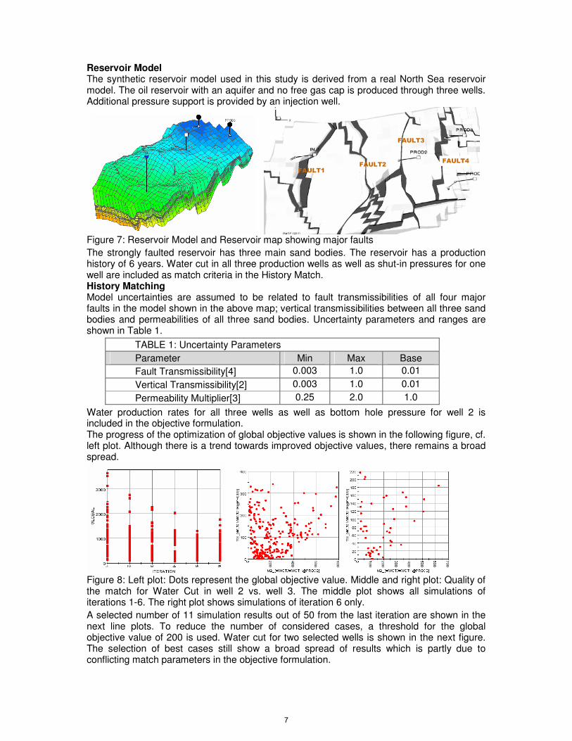
Figure 5: Red dots represent the global objective function values, yellow and blue dots the partial contributions f1 and f2 respectively. The first 50 simulation runs are part of the initialization run and show a wide spread of values. For the minimization problem the Optimizer is intended to find the smallest objective value. Due to conflicting objectives in f1 and f2, there is a continuous broad band of results for all subsequent iterations. No clear convergence trend is seen, which is representative for multi-objective optimization problems. The following plots give a different focus on the same set of data. Each plot shows f1 vs. f2. Plot 1 on the left side includes all results for the initialization run. A broad spread of data is seen. Plot 2 is taken from iteration 3, i.e. simulation runs 151 to 200. It already reveals a clear front which is further refined in iteration 6 shown in plot 3. Plot 4 on the right side includes all simulation runs, including the initialization run. The Pareto front shown in plots 2-4 is a good approximation to the analytical front of Equation (6). It is not possible to improve the result any further than defined by the Pareto front. At the same time, the Pareto optimizer has kept a broad spread of results on the Pareto front which guarantees a diversity of results. Based on these observations the Pareto Optimizer meets the two major design criteria described above.

1 2

f1 f1

f2

f2

43

f1 f1

f2 f2

Figure 6: Solution space shown for different iterations as part of the optimization process.

History Matching Application

This section discusses the application of the Pareto Optimizer to a reservoir simulation case.

6

Reservoir Model The synthetic reservoir model used in this study is derived from a real North Sea reservoir model. The oil reservoir with an aquifer and no free gas cap is produced through three wells. Additional pressure support is provided by an injection well.

FAULT1

FAULT2

FAULT3

FAULT4

Figure 7: Reservoir Model and Reservoir map showing major faults The strongly faulted reservoir has three main sand bodies. The reservoir has a production history of 6 years. Water cut in all three production wells as well as shut-in pressures for one well are included as match criteria in the History Match. History Matching Model uncertainties are assumed to be related to fault transmissibilities of all four major faults in the model shown in the above map; vertical transmissibilities between all three sand bodies and permeabilities of all three sand bodies. Uncertainty parameters and ranges are shown in Table 1.

TABLE 1: Uncertainty Parameters Parameter Min Max Base Fault Transmissibility[4] 0.003 1.0 0.01

Vertical Transmissibility[2] 0.003 1.0 0.01

Permeability Multiplier[3] 0.25 2.0 1.0

Water production rates for all three wells as well as bottom hole pressure for well 2 is included in the objective formulation. The progress of the optimization of global objective values is shown in the following figure, cf. left plot. Although there is a trend towards improved objective values, there remains a broad spread.

Figure 8: Left plot: Dots represent the global objective value. Middle and right plot: Quality of the match for Water Cut in well 2 vs. well 3. The middle plot shows all simulations of iterations 1-6. The right plot shows simulations of iteration 6 only. A selected number of 11 simulation results out of 50 from the last iteration are shown in the next line plots. To reduce the number of considered cases, a threshold for the global objective value of 200 is used. Water cut for two selected wells is shown in the next figure. The selection of best cases still show a broad spread of results which is partly due to conflicting match parameters in the objective formulation.

7

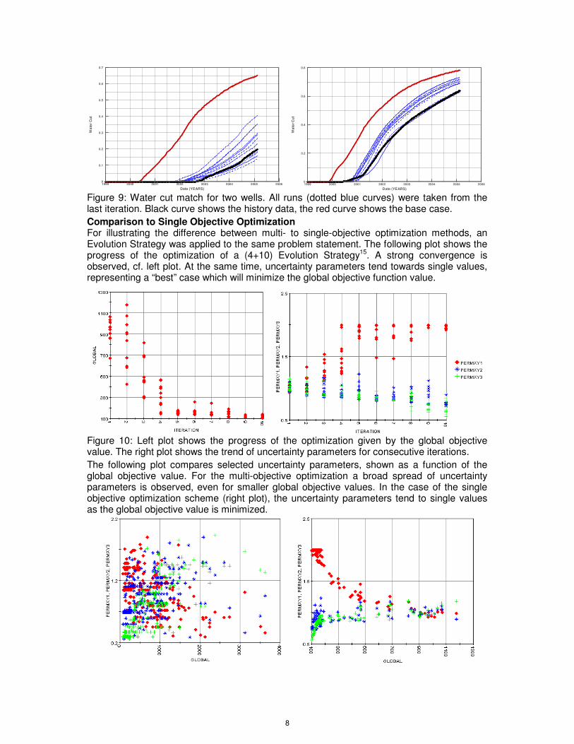
Figure 9: Water cut match for two wells. All runs (dotted blue curves) were taken from the last iteration. Black curve shows the history data, the red curve shows the base case. Comparison to Single Objective Optimization For illustrating the difference between multi- to single-objective optimization methods, an Evolution Strategy was applied to the same problem statement. The following plot shows the progress of the optimization of a (4+10) Evolution Strategy15. A strong convergence is observed, cf. left plot. At the same time, uncertainty parameters tend towards single values, representing a “best” case which will minimize the global objective function value.

Figure 10: Left plot shows the progress of the optimization given by the global objective value. The right plot shows the trend of uncertainty parameters for consecutive iterations. The following plot compares selected uncertainty parameters, shown as a function of the global objective value. For the multi-objective optimization a broad spread of uncertainty parameters is observed, even for smaller global objective values. In the case of the single objective optimization scheme (right plot), the uncertainty parameters tend to single values as the global objective value is minimized.

Date (YEARS)

Wa

ter

Cu

t

1999 2000 2001 2002 2003 2004 2005 20060

0.2

0.4

0.6

0.8

Date (YEARS)

Wa

ter

Cu

t

1999 2000 2001 2002 2003 2004 2005 20060

0.1

0.2

0.3

0.4

0.5

0.6

0.7

8

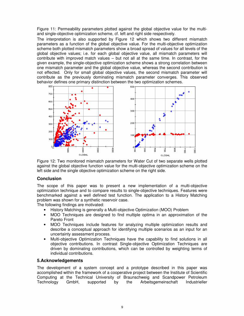
Figure 11: Permeability parameters plotted against the global objective value for the multi-and single-objective optimization scheme, cf. left and right side respectively. The interpretation is also supported by Figure 12 which shows two different mismatch parameters as a function of the global objective value. For the multi-objective optimization scheme both plotted mismatch parameters show a broad spread of values for all levels of the global objective values; i.e. for each global objective value, all mismatch parameters will contribute with improved match values – but not all at the same time. In contrast, for the given example, the single-objective optimization scheme shows a strong correlation between one mismatch parameter and the global objective value, whereas the second contribution is not effected. Only for small global objective values, the second mismatch parameter will contribute as the previously dominating mismatch parameter converges. This observed behavior defines one primary distinction between the two optimization schemes.

Figure 12: Two monitored mismatch parameters for Water Cut of two separate wells plotted against the global objective function value for the multi-objective optimization scheme on the left side and the single objective optimization scheme on the right side.

Conclusion

The scope of this paper was to present a new implementation of a multi-objective optimization technique and to compare results to single-objective techniques. Features were benchmarked against a well defined test function. The application to a History Matching problem was shown for a synthetic reservoir case. The following findings are motivated:

• History Matching is generally a Multi-objective Optimization (MOO) Problem • MOO Techniques are designed to find multiple optima in an approximation of the

Pareto Front • MOO Techniques include features for analyzing multiple optimization results and

describe a conceptual approach for identifying multiple scenarios as an input for an uncertainty assessment process.

• Multi-objective Optimization Techniques have the capability to find solutions in all objective contributions. In contrast Single-objective Optimization Techniques are driven by dominating contributions, which can be controlled by weighting terms of individual contributions.

5.Acknowledgements

The development of a system concept and a prototype described in this paper was accomplished within the framework of a cooperative project between the Institute of Scientific Computing at the Technical University of Braunschweig and Scandpower Petroleum Technology GmbH, supported by the Arbeitsgemeinschaft Industrieller

9

Forschungsvereinigungen [Organization of Industrial Research Associations] (AIF) under contract numbers KF 0250701SS5 and KF0259501SS5. The authors wish to thank Oliver Pajonk from the Institute of Scientific Computing, who has supported the implementation of the link between the Pareto Optimizer and MEPO. We also like to thank Stefan Djupvik, Scandpower Petroleum Technology who has provided the reservoir test case used in this study.

6.References

1. S.Begg, R.B. Bratvold, J.M.Campbell: “Improving Investment Decisions Using a Stochastic Asset

Model,” paper SPE71414 prepared for the Annual Technical Conference and Exhibition, New

Orleans, 30 September – 3 October, 2001

2. Tarantola, A.: Inverse Problem Theory – Methods for Data Fitting and Model Parameter

Estimation, Elsevier, Amsterdam (1987)

3. Lande, J.L., Kalia, R.K., Nakano, A., Nomura, K., Vashishta, P.: “History Match and Associated

Forecast Uncertainty Analysis – Practical Approaches Using Cluster Computing”, paper

IPTC10751 presented at the IPTC 2005, Doha, Qatar, 21-23 November 2005

4. Krosche, M., Axmann, J.K., Pajonk, O., Schulze-Riegert, R., Haase, O.: “A Software Component

Based Parallel Simulation and Optimization Environment for Reservoir Simulation,” Proceedings

of the DGMK Spring Conference 2005, ISBN 3-936418-35--7

5. SPE Applied Technology Workshop, “History Matching: New Developments and Best Practices”,

Houston, Texas, 18-20 Oct. 2006

6. G.J.J. Williams, M. Mansfield, D.G. MacDonald, M.D. Bush: “Top-Down Reservoir Modelling,”

paper SPE89974 presented at the ATCE 2004, Houston, Texas, 26-29. Sep. 2004

7. G.J. Walker, & S. Pettigrew; “Measures of Efficiency for Assisted History Matching,” 10th

European Conference on the Mathematics of Oil Recovery — Amsterdam, The Netherlands 4 - 7

September 2006

8. A. Castellini*, B. Yeten, U. Singh, A. Vahedi, R. Sawiris; “History Matching and Uncertainty

Quantification Assisted by Global Optimization Techniques,” 10th European Conference on the

Mathematics of Oil Recovery — Amsterdam, The Netherlands 4 - 7 September 2006

9. M. Rotondi, G. Nicotra, A. Godi, F.M. Contento, M.J. Blunt, M.A. Christie: “Hydrocarbon

Production Forecast and Uncertainty Quantification: A Field Application,” paper SPE102135

prepared for the Annual Technical Conference and Exhibition, San Antonio, 24-27 September,

2006

10. C.A. Coello, D.A. Veldhuizen, G.B. Lamont: Evolutionary Algorithms for Solving Multi-Objective

Problems. Kluwer, New York, 2002

11. K.Deb; Multi-Objective optimization using evolutionary algorithms. Wiley, Chichester, UK, 2001

12. C.M. Fonseca, P.J. Fleming; Genetic algorithms for multi-objective optimization: Formulation,

discussion and generalization, Proceedings of the Fifth International Conference on Genetic

Algorithms. Pages 416-423. 1993.

13. Goldberg, D.E.: Genetic Algorithms in Search, Optimization and Machine Learning, Addision-

Wesley, Reading (1989)

14. Bäck, T.: Evolutionary Algorithms in Theory and Practice, Oxford University Press, Oxford (1996)

15. R.W. Schulze-Riegert, J.K. Axmann, O. Haase, D.T. Rian, Y.-L. You.: “Evolutionary Algorithms

Applied to History Matching of Complex Reservoirs,” SPE Reservoir Evaluation & Engineering

(Apr. 2002) 5 (2)

16. R. Schulze-Riegert, M. Krosche, A. Fahimuddin, S. Ghedan: “Multi-Objective Optimization with

Application to Model Validation and Uncertainty Quantification,” paper SPE105313 prepared for

presentation at the 15th SPE Middle East Oil & Gas Show and Conference held in Bahrain

International Exhibition Centre, Kingdom of Bahrain, 11–14 March 2007

17. E. Zitzler, M. Laumanns, L. Thiele; SPEA2: Improving the strength pareto evolutionary algorithm

for multiobjective optimization. CIMNE Evolutionary Methods for Design, Optimisation and

Control, pages 19-26, Barcelona, Spain, 2002.

18. J. Horn, N. Nafploitis, D.E. Goldberg; A niched Pareto genetic algorithm for multi-objective

optimization, Proceedings of the First IEEE Conference on Evolutionary Computations, pages 82-

87, 1994.

10