HAL Id: hal-03425550 https://hal.archives-ouvertes.fr/hal-03425550 Submitted on 17 Nov 2021 HAL is a multi-disciplinary open access archive for the deposit and dissemination of sci- entific research documents, whether they are pub- lished or not. The documents may come from teaching and research institutions in France or abroad, or from public or private research centers. L’archive ouverte pluridisciplinaire HAL, est destinée au dépôt et à la diffusion de documents scientifiques de niveau recherche, publiés ou non, émanant des établissements d’enseignement et de recherche français ou étrangers, des laboratoires publics ou privés. Global reference seismological datasets: Multi-mode surface wave dispersion P Moulik, V Lekic, B Romanowicz, Z Ma, A Schaeffer, T Ho, E Beucler, E Debayle, A Deuss, S Durand, et al. To cite this version: P Moulik, V Lekic, B Romanowicz, Z Ma, A Schaeffer, et al.. Global reference seismological datasets: Multi-mode surface wave dispersion. Geophysical Journal International, Oxford University Press (OUP), 2021, 10.1093/gji/ggab418. hal-03425550

Welcome message from author
This document is posted to help you gain knowledge. Please leave a comment to let me know what you think about it! Share it to your friends and learn new things together.
Transcript
HAL Id: hal-03425550https://hal.archives-ouvertes.fr/hal-03425550
Submitted on 17 Nov 2021
HAL is a multi-disciplinary open accessarchive for the deposit and dissemination of sci-entific research documents, whether they are pub-lished or not. The documents may come fromteaching and research institutions in France orabroad, or from public or private research centers.
L’archive ouverte pluridisciplinaire HAL, estdestinée au dépôt et à la diffusion de documentsscientifiques de niveau recherche, publiés ou non,émanant des établissements d’enseignement et derecherche français ou étrangers, des laboratoirespublics ou privés.
Global reference seismological datasets: Multi-modesurface wave dispersion
P Moulik, V Lekic, B Romanowicz, Z Ma, A Schaeffer, T Ho, E Beucler, EDebayle, A Deuss, S Durand, et al.
To cite this version:P Moulik, V Lekic, B Romanowicz, Z Ma, A Schaeffer, et al.. Global reference seismological datasets:Multi-mode surface wave dispersion. Geophysical Journal International, Oxford University Press(OUP), 2021, 10.1093/gji/ggab418. hal-03425550
submitted to Geophys. J. Int.
Global Reference Seismological Datasets: Multi-mode
Surface Wave Dispersion
P. Moulik1?, V. Lekic1, B. Romanowicz2,3,4, Z. Ma5, A. Schaeffer6, T. Ho7
E. Beucler8, E. Debayle9, A. Deuss10, S. Durand9, G. Ekstrom11, S. Lebedev7,12
G. Masters13, K. Priestley7, J. Ritsema14, K. Sigloch15, J. Trampert10, A.M. Dziewonski16†
1Department of Geology, University of Maryland, College Park, MD 20742, USA
2Berkeley Seismological Laboratory, McCone Hall, University of California, Berkeley, CA 94720, USA
3Institut de Physique du Globe de Paris, 1 Rue Jussieu, F-752382 Paris Cedex 05, France
4College de France, 11 Place Marcelin Berthelot, F-75005 Paris, France
5State Key Laboratory of Marine Geology, Tongji University, Shanghai, 200092, China
6Geological Survey of Canada, Pacific Division, Sidney, BC V8L 4B2, Canada
7Department of Earth Sciences, Bullard Laboratories, University of Cambridge, Cambridge CB3 0EZ, United Kingdom
8Laboratoire de Planetologie et de Geodynamique, Nantes University, UMR-CNRS 6112, BP92208 F-44322 Nantes, France
9Laboratoire de Geologie de Lyon-Terre, Planete, Environnement, CNRS UMR 5276, Ecole Normale Superieure de Lyon, Universite de Lyon, Universite Claude Bernard Lyon 1, Villeurbanne, France
10Department of Earth Sciences, Utrecht University, Princetonlaan 8a, 3584 CB Utrecht, The Netherlands
11Lamont-Doherty Earth Observatory of Columbia University, Palisades, NY 10964, USA
12Geophysics Section, School of Cosmic Physics, Dublin Institute for Advanced Studies, Dublin, Ireland
13Scripps Institution of Oceanography, University of California San Diego, La Jolla, CA 92093, USA
14Department of Earth and Environmental Sciences, University of Michigan, Ann Arbor, Michigan, USA
15Department of Earth Sciences, University of Oxford, Oxford OX1 3PR, UK
16Department of Earth and Planetary Sciences, Harvard University, Cambridge, MA 02138, USA

2 P. Moulik et al.
1
SUMMARY2
Global variations in the propagation of fundamental-mode and overtone surface waves3
provide unique constraints on the low-frequency source properties and structure of the4
Earth’s upper mantle, transition zone and mid mantle. We construct a reference dataset5
of multi-mode dispersion measurements by reconciling large and diverse catalogs of6
Love-wave (49.65 million) and Rayleigh-wave dispersion (177.66 million) from 8 groups7
worldwide. The reference dataset summarizes measurements of dispersion of fundamental-8
mode surface waves and up to six overtone branches from 44871 earthquakes recorded on9
12222 globally distributed seismographic stations. Dispersion curves are specified at a set10
of reference periods between 25 and 250 s to determine propagation-phase anomalies with11
respect to a reference Earth model. Our procedures for reconciling datasets include: (1)12
controlling quality and salvaging missing metadata; (2) identifying discrepant measure-13
ments and reasons for discrepancies; (3) equalizing geographic coverage by constructing14
summary rays for travel-time observations; and (4) constructing phase velocity maps at15
various wavelengths with combination of data types to evaluate inter-dataset consistency.16
We retrieved missing station and earthquake metadata in several legacy compilations and17
codified scalable formats to facilitate reproducibility, easy storage and fast input/output18
on high-performance-computing systems. Outliers can be attributed to cycle skipping,19
station polarity issues or overtone interference at specific epicentral distances. By assess-20
ing inter-dataset consistency across similar paths, we empirically quantified uncertain-21
ties in travel-time measurements. More than 95% measurements of fundamental-mode22
dispersion are internally consistent, but agreement deteriorates for overtones especially23
branches 5 and 6. Systematic discrepancies between raw phase anomalies from vari-24
ous techniques can be attributed to discrepant theoretical approximations, reference Earth25
models and processing schemes. Phase-velocity variations yielded by the inversion of the26
summary dataset are highly correlated (R ≥ 0.8) with those from the quality-controlled27
contributing datasets. Long-wavelength variations in fundamental-mode dispersion (50–28
100 s) are largely independent of the measurement technique with high correlations ex-29

Global Reference Seismological Datasets: Surface Waves 3
tending up to degree ∼ 25. Agreement degrades with increasing branch number and30
period; highly correlated structure is found only up to degree ∼ 10 at longer periods31
(T > 150 s) and up to degree ∼ 8 for overtones. Only 2ζ azimuthal variations in phase32
velocity of fundamental-mode Rayleigh waves were required by the reference dataset;33
maps of 2ζ azimuthal variations are highly consistent between catalogs (R = 0.6–0.8).34
Reference data with uncertainties are useful for improving existing measurement tech-35
niques, validating models of interior structure, calculating teleseismic data corrections in36
local or multi-scale investigations, and developing a 3D reference Earth model.37
Key words: Computational seismology, Mantle processes, Surface waves and free oscil-38
lations, Seismic anisotropy, Seismic tomography.39
1 INTRODUCTION40
A fundamental goal in seismology is to accurately determine the elastic structure of the Earth’s interior.41
Elastic reference models are widely used in the geosciences for the modeling and interpretation of42
seismic sources and planetary interiors. Earth’s interior has traditionally been described in terms of43
spherically symmetric (1D) structure with physical properties varying radially within concentric shells44
such as the upper mantle and outer core. It is now well established that there are substantial three-45
dimensional (3D) variations in the mantle and that 3D tomographic models are useful as starting46
models for more detailed imaging studies and in constraining physical parameters such as temperature,47
grain size, fabric and composition. While radial (1D) reference Earth models have been available for48
several decades (e.g. Dziewonski & Anderson 1981; Kennett et al. 1995), only recently has global49
seismic imaging reached a point where the development of a 3D reference Earth model (REM3D)50
can be envisaged. A key component in this endeavor is to accurately characterize the arrival times of51
various phases observed on broadband seismograms.52
Surface waves are the most prominent phases recorded at teleseismic distances at periods longer53
than 30 s, especially from shallow-focus earthquakes. Two types of surface waves are observed, distin-54
guished by their polarization during propagation through the Earth: Love (SH) and Rayleigh (P-SV)55
waves, recorded on the transverse and vertical/longitudinal components, respectively. Surface-wave56
? Corresponding author. Now at the Department of Geosciences, Princeton University, Princeton, NJ 08544, USA. E-mail:
[email protected]† deceased
4 P. Moulik et al.
arrivals are denoted by the orbit number (e.g. No = 1 for minor-arc L1 or R1 waves), a proxy for the57
number of times the wave circles around the Earth (Nc = [No-1]⁄2 for odd No, No⁄2 otherwise). The wave58
trains excited by large mega-thrust earthquakes (Mw ≥ 7.5) circle the Earth multiple times (Nc ≥ 1)59
for many hours and manifest as discernible higher-orbit arrivals (e.g. L3–L5, R3–R5). Generation60
and propagation of surface waves can also be classified based on the properties of the correspond-61
ing normal modes. Fundamental-mode surface wave trains are excited more strongly by shallow and62
intermediate-depth earthquakes (h < 250 km) and appear well separated from other phases at tele-63
seismic distances (∆ > 30). Higher-mode or overtone vibrations are excited by deeper earthquakes64
and appear as faster propagating, compact wave packets that contribute to the long-period body wave-65
forms (e.g. Takeuchi & Saito 1972). Characterizing surface waves and overtones is critical for the66
construction of elastic reference Earth models.67
In addition to their large amplitudes, surface waves are characterized by a frequency-dependence68
of velocity (i.e. dispersion). In cohort with other complementary datasets, laterally variable dispersion69
resulting from structural heterogeneity is crucial for mapping the upper mantle, transition zone and70
mid mantle (e.g. Masters et al. 2000; Ritsema et al. 2004; Moulik & Ekstrom 2014). Accounting for71
dispersion is also useful for locating earthquakes (e.g. Ekstrom 2006b; Howe et al. 2019), signal en-72
hancement through phase-coherent stacking of seismograms (e.g. Ma et al. 2014), and inverting the73
centroid-moment tensors (CMTs) of seismic sources (Dziewonski et al. 1981; Ekstrom et al. 2005).74
Several techniques have been employed to directly or indirectly measure dispersion of fundamental-75
mode surface waves and overtones (e.g. Dziewonski et al. 1972; Herrin & Goforth 1977; Lerner-Lam76
& Jordan 1983; Cara & Leveque 1987; Stutzmann & Montagner 1993; Trampert & Woodhouse 1995;77
Ekstrom et al. 1997; van Heijst & Woodhouse 1997; Debayle 1999; Yoshizawa & Kennett 2002a;78
Beucler et al. 2003; Lebedev et al. 2005; Visser et al. 2007; Ma et al. 2014). These techniques em-79
ploy various processing and fitting procedures with different assumptions on crustal structure, mode80
coupling, reference model, geodetic parameters, and attenuation. To date, no systematic assessment of81
the consistency in the resulting measurements has been performed. Such comparisons can help iden-82
tify outliers or systematic biases and provide method-agnostic estimates of measurement uncertainty.83
Reference datasets with uncertainties are crucial for testing hypotheses about mantle structure, such84
as those concerning the depth and lateral variations of radial and azimuthal anisotropy (e.g. Trampert85
& Woodhouse 2003; Visser & Trampert 2008; Ekstrom 2011; Ma et al. 2014; Schaeffer et al. 2016).86
Additionally, inversions based on the reconciled reference dataset can inform parametrization and reg-87
ularization choices that strongly impact the inferences of mantle structure (e.g. Spetzler et al. 2002;88
Sieminski et al. 2004; Boschi et al. 2006; van der Hilst & de Hoop 2005; Trampert & Spetzler 2006).89
This is the first in a series of papers that describe a community effort to construct a 3D reference90

Global Reference Seismological Datasets: Surface Waves 5
model (REM3D) for the Earth’s mantle. A major objective is to provide quality-controlled, compre-91
hensive and publicly-available seismological datasets with corresponding uncertainties. Towards this92
goal, we openly solicited contributions and feedback on recent surface-wave measurements between93
the years 2014–2020; eight groups across the world responded and contributed recent, updated and/or94
unpublished measurements (Table 1, Figure 1). In this paper, we present the results of our efforts to95
construct a reference dataset for surface wave dispersion measurements, which traditionally constitute96
a major ingredient for constraining large scale upper mantle structure. The scope of this paper is de-97
liberately limited. We quantified the consistency across the eight contributed large catalogs of diverse98
surface-wave dispersion measurements and constructed a reference dataset with uncertainties. Phase-99
velocity maps were derived at a prescribed set of frequencies, and demonstrate the strong inter-catalog100
agreement on inferred structure. We did not explore the implications of these phase-velocity variations101
for Earth structure to any significant extent. Natural continuations of this work are a comparison of102
dispersion predicted from 3D tomographic models with the reference dataset, and the determination103
of a 3D reference Earth model (REM3D) that can provide accurate dispersion predictions across all104
overtone branches.105
We first summarize basic definitions and theoretical assumptions of surface-wave propagation106
employed in this study (Sections 2–3). A summary of the contributed data, measurement techniques107
and our processing scheme is outlined in Section 4. We use a standard processing scheme to reconcile108
the large catalogs of surface-wave dispersion measurements contributed to this study (Figure 2). The109
major steps include pre-processing, metadata analysis, homogenization, quality control, inter-catalog110
comparisons, outlier analysis, and construction of the reference data set with uncertainties (Sections 4–111
5). For clarity, the names of datasets obtained during the various stages of our processing scheme112
(Figure 2) are denoted in italics in the rest of this paper. Finally, we explore the implications on Earth113
structure (Section 6) and conclude with a discussion of the results (Section 7).114
2 BACKGROUND115
Propagation velocities of surface waves on a sphere depend on frequency, a property called dispersion,116
which, to first order, can reflect the variation with depth of Earth’s elastic structure. The early surface-117
wave studies focused on fundamental mode dispersion in narrow frequency bands (∼30–100 s) along118
certain paths or across tectonically contiguous regions using the phase difference between two stations119
aligned with the source to eliminate source contributions (e.g. Tams 1921; Oliver 1962; Toksoz &120
Anderson 1966; Dorman 1969; Brune 1970; Kanamori 1970; Knopoff 1972). The separation of surface121
wave overtones, which appear as compact wavepackets that arrive ahead of the fundamental mode,122
requires more sophistication, with early methodologies making use of array measurements (e.g. Cara123
6 P. Moulik et al.
& Hatzfeld 1977; Nolet 1977). Measurement of overtone dispersion is important, as their sensitivity to124
structure, at a given frequency, extends to greater depths in the mantle than fundamental-mode surface125
waves.126
Since the 1980s, rapid progress has been made in surface-wave seismology due to the prolifera-127
tion of digital broadband seismographic networks (e.g. Agnew et al. 1976; Peterson et al. 1976; Ro-128
manowicz et al. 1991). Combined with theoretical and methodological improvements, this has made129
it possible to develop global maps of fundamental mode surface wave dispersion (Nakanishi & An-130
derson 1982; Montagner & Tanimoto 1991; Shapiro & Ritzwoller 2002; Ekstrom 2011), extend the131
range of measurements to shorter periods (e.g. Trampert & Woodhouse 1995; Zhang & Lay 1996;132
Ekstrom et al. 1997; Yoshizawa & Kennett 2002a), and obtain global dispersion measurements of133
overtones (e.g. Stutzmann & Montagner 1993; van Heijst & Woodhouse 1997; Debayle 1999; Beucler134
et al. 2003; Lebedev et al. 2005; Visser et al. 2007). Phase velocity maps are now a routine tool in135
regional and global investigations of crust and mantle structure. The procedure typically comprises136
two steps: 1) inverting an ensemble of path-specific dispersion measurements for maps of the dis-137
tribution of phase or group velocity at a given frequency, a linear process; 2) inverting the obtained138
dispersion curve beneath a given geographical location for elastic structure as a function of depth, a139
non-linear process generally performed in the context of a simple approximation to first-order normal140
mode perturbation theory.141
Fundamental-mode and overtone wave trains can also be inverted directly for three-dimensional142
(3D) structure. Such formulations rely on a normal mode perturbation formalism that took advantage143
of the equivalence of surface waves and normal modes in the asymptotic limit of high frequency144
(e.g. Gilbert 1976; Mochizuki 1986; Romanowicz 1987), including different levels of approximation145
(e.g. Woodhouse & Dziewonski 1984; Nolet 1990; Li & Romanowicz 1995; Marquering et al. 1999),146
and culminating recently with the introduction of the Spectral Element Method (e.g. Komatitsch &147
Vilotte 1998; Komatitsch & Tromp 1999) in global tomography (e.g. Lekic & Romanowicz 2011;148
French & Romanowicz 2014; Bozdag et al. 2016). Although waveform inversion is not the topic149
of this paper, various approximations for the computation of the predicted wavefield are relevant to150
modern dispersion measurement methods (Section 4.2). Reviews of the basic properties, techniques151
for surface waves and inferences on structure can be found elsewhere (e.g. Stein & Wysession 2009;152
Romanowicz 2002). We summarize below the theoretical and observational aspects most pertinent to153
the construction of a reference dataset.154
Global Reference Seismological Datasets: Surface Waves 7
3 THEORETICAL FRAMEWORK155
The propagation of seismic surface waves was first developed in the framework of a flat, layered model
of the Earth, to which corrections for sphericity are applied at far regional and teleseismic distances.
Later, the equivalence between a propagating surface wave formalism and a normal mode formalism
in a spherically symmetric Earth model, was established (e.g. Gilbert 1976; Aki & Richards 1980).
Given the ensemble of Rayleigh (or Love) wavetrains propagating along a great circle path, we denote
the successive surface wavetrains propagating in the direction of the minor arc from the source to the
receiver as R1, R3, R5 (or L1, L3, L5) and those propagating in the opposite direction as R2, R4, R6
(or L2, L4, L6). Surface wavetrains can be interpreted in terms of Rayleigh-wave equivalent spheroidal
modes nSl or Love-wave equivalent toroidal modes nTl with radial order n and angular order l. For a
particular mode type (spheroidal S or toroidal T ), the displacement time series recorded at the receiver
r can be expressed as a sum over normal modes as follows:
u(r, t) =∑k
uk(t) =∑n
∑l
nAl · einωlt, (1)
where nωl is the complex eigenfrequency of the mode, and nAl is its excitation amplitude for the
particular source-station configuration. Alternatively, the displacement time series can be expressed,
in the high frequency limit, as a sum of propagating surface waves as:
u(r, ω) ≈∑n
An(ω) · eiΦn(ω), (2)
where An(ω) and Φn(ω) are the amplitude and phase of the nth surface wave overtone as a function156
of angular frequency ω (Aki & Richards 1980).157
Dropping the overtone index n, the phase Φ for a particular source receiver pair comprises four
contributions in a spherically symmetric Earth model
Φ = ΦS + ΦR +Mπ
2+ ΦP , (3)
where ΦS is the contribution from the source, ΦR is the receiver phase shift, ΦP is the contribution
to the phase due to propagation from the source to the receiver, and M is a signed integer, which
represents the number of passages through the source antipode (e.g. M = 0 for R1 and L1, M = 1 for
R3 and L3, M = -1 for R2 and L2). Similarly, the amplitude term An(ω) can be decomposed into a
product of contributions:
An = ASARAFAQ, (4)
where AS is the magnitude of the excitation at the source, AR is the receiver amplification, AF is the
geometrical spreading factor, and AQ is the decay factor due to anelastic attenuation along the ray

8 P. Moulik et al.
path. The propagation phase is defined in terms of a phase velocity C(ω) as
ΦP (ω) =ωX
C(ω)(5)
where X is the distance traveled by the wave. When we assume propagation to follow the great circle
path,X equals ∆, the great-circle distance that is calculated using a distance factor (∆F = 111.31948)
after applying the geocentric conversion factor (W = 0.9933056) to the locations in geographic co-
ordinates (e.g. Seidelmann 1992; Moulik & Ekstrom 2021). In a spherically symmetric Earth model,
C(ω) does not depend on the source-station geometry. For a given mode branch n, phase velocity is
related to the corresponding mode eigenfrequency as
C(nωl) =nωl ·Rl + 1/2
, (6)
where R = 6371 km is the mean radius of the Earth (Jeans 1927).158
In the 3D Earth, the phase velocity measured on a given source-station path depends on the lo-
cation of the source and station, and on the source radiation pattern to account for potential off-great
circle propagation. A common assumption made in interpreting phase velocity measurements is the
‘path average’ approximation (PAVA, Woodhouse & Dziewonski 1984). Propagation is assumed to
occur along the great circle path, and the propagating phase only depends on the distance between the
source and receiver. Given a reference spherically symmetric Earth model, in which the phase velocity
for a given surface wave branch is C0(ω) (or its inverse, the phase slowness P0(ω)), the propagation
phase in the reference model is:
Φ0P =
ω∆
C0= ω∆P0 (7)
and the measured propagation phase ΦP between two points distant by ∆ can then be written as
ΦP (ω) = Φ0P (ω) + δΦP =
ω∆
(C0 + δC)+ S · 2π = ω∆(P0 + δP ) + S · 2π, (8)
where δC and δP are the perturbations in phase velocity and slowness, respectively, due to variations
in velocity away from the reference spherically symmetric model. The integer S accounts for inde-
terminacy due to the definition of phase modulo 2π. The varying structure along the path s is most
conveniently described by ‘local’ phase slowness perturbations δp(ω, s), such that
δΦP = ω
∫path
δp(ω, s)ds+ S · 2π. (9)
Note that care must be taken to avoid ‘cycle skipping’ when inferring the slowness perturbation159
δP . Since the differences in dispersion between the predictions from a reference 1-D model and the160
real observations are small at long periods (>100s), there is usually no ambiguity in the selection of S.161
Most surface wave dispersion studies start processing at longer periods, so that continuous dispersion162
Global Reference Seismological Datasets: Surface Waves 9
curves can be anchored, and the total phase perturbation at shorter periods can be inferred with less163
ambiguity. Of particular interest to this study is the distribution of local phase slowness δp(ω, s) and164
its inverse, phase velocity δc(ω, s) at a given frequency and mode branch. Such two-dimensional (2D)165
maps can be derived by the inversion of measured phase slowness perturbations δP (ω) over many166
source-station paths, while potentially including measurements on higher orbits. The resulting phase167
dispersion curves obtained over a band of frequencies at each point on the Earth’s surface can be168
inverted in turn for elastic structure as a function of depth, using sensitivity kernels derived from169
normal mode perturbation theory or fully numerical approaches.170
The perturbation in phase velocity at a fixed frequency ω is related to the perturbation in local
eigenfrequency at a fixed wavenumber k as(δc
c0
)ω
=c0
U0
(δω
ω0
)k
, (10)
where U is the group velocity (e.g. Dahlen & Tromp 1998). While it is straightforward to derive171
equation 9 for surface waves in the frequency domain, relating it to normal mode perturbation theory172
took some theoretical development. Simply perturbing the eigenfrequency of a mode only allows us173
to represent the effect of heterogeneity integrated over the entire great circle path (e.g. Jordan 1978),174
and therefore sensitivity to structure that is symmetric with respect to the center of the Earth (‘even175
order’ heterogeneity). It can be shown that the PAVA approximation for surface waves is equivalent to176
along-branch mode coupling in the asymptotic limit of large angular orders of first order perturbation177
theory applied to normal modes (Mochizuki 1986; Park 1987; Romanowicz 1987). The along-branch178
coupling brings out the sensitivity of the modes to odd-order heterogeneity. Most surface wave and179
overtone phase dispersion measurement techniques implicitly utilize the PAVA approximation to relate180
3D structural heterogeneity at depth to observed slownesses. In the rest of the paper, we will use the181
great-circle ray approximation (GCRA), which is a related infinite-frequency approximation that pre-182
dicts phase delays from 2D slowness maps without accounting for finite-frequency (e.g. FFT, Wang &183
Dahlen 1995b; Yoshizawa & Kennett 2002b; Zhou et al. 2004) or off-great-circle propagation effects184
adopted in exact ray theory (e.g. ERT, Woodhouse & Wong 1986; Larson et al. 1998). Similar struc-185
tures can be obtained using GCRA, FFT and ERT theory depending on the choices of parameterization186
and regularization (Spetzler et al. 2002; Sieminski et al. 2004; Boschi et al. 2006; Trampert & Spet-187
zler 2006). Based on synthetic experiments, GCRA accurately predicts phase anomalies of minor-arc188
phases and matches input phase slowness maps at global scales (e.g. Godfrey et al. 2019). The basic189
assumption in GCRA that rays travel along the great circle connecting the source and receiver may190
become less valid with increasing path length (e.g. Woodhouse & Wong 1986), such as in the case of191
higher-orbit measurements (L3–L5, R3–R5). A detailed comparison of theoretical assumptions for all192
10 P. Moulik et al.
wave types is beyond the scope of this study. However, we note that Wang & Dahlen (1995b) found193
little dependence of errors in the ERT approximation on the orbit number of surface waves.194
4 DATA195
4.1 Compilation196
Our compilation included global catalogs of dispersion data measured by 8 groups with domain exper-197
tise in processing surface-wave observations with a variety of techniques (Table 1). The contributed198
compilation consisted of 49.65 million Love-wave and 177.66 million Rayleigh-wave measurements199
for a total of Ncontrib ∼ 227 million estimates of frequency-dependent propagation phase for various200
overtone branches. The following papers describe the underlying methodology of each contributed201
dataset in more detail: Cambridge19 (Debayle & Ricard 2012; Ho et al. 2016); Dublin13 (Lebedev202
et al. 2005; Schaeffer & Lebedev 2013); GDM52 (Ekstrom et al. 1997; Ekstrom 2011); IPGP03 (Stutz-203
mann & Montagner 1994; Beucler et al. 2003; Beucler & Montagner 2006); Lyon18 (Debayle 1999;204
Debayle & Ricard 2012); MBS11 (van Heijst & Woodhouse 1997; Ritsema et al. 2011); Scripps14205
(Ma et al. 2014); Utrecht08 (Yoshizawa & Kennett 2002a; Visser et al. 2007). Fundamental-mode206
(n = 0), minor-arc (L1, R1) measurements were the most common type of data across the 8 contribu-207
tions. Additional constraints on major-arc arrivals (L2, R2) were available from two sources (GDM52,208
MBS11), while higher-orbit measurements (L3–L5, R3–R5) were included from GDM52. All groups209
contributed measurements in terms of path-dependent dispersion curves for various overtone branches210
(n = 0–18) sampled unevenly at different sets of discrete frequencies. The contributions included mea-211
surements from recent analyses and unpublished updates in formats that accounted for the processing212
guidelines in this study (Section 4.3, Appendix A). Rayleigh-wave dispersion data on the vertical213
component are more widely available (>3 times) than Love-wave measurements due to the inherently214
noisier records on the horizontal component seismograms. The contributed compilation represents the215
largest and most diverse set of surface-wave arrival times assembled to date.216
Figure 1 shows the reported locations of 44871 sources and 12222 receivers that contributed at217
least one observation to this study. Waveform data for the majority of catalogs were available from the218
Incorporated Research Institutions for Seismology (IRIS). All catalogs adopted in their measurement219
procedure the source mechanisms (CMTs) from the Global CMT project (Dziewonski et al. 1981;220
Ekstrom et al. 2005) in their measurement procedure. Recent implementations of the Global CMT221
algorithm minimizes the difference between observed and synthetic seismograms in three frequency222
bands and time windows. These include the body waves (40–150 s), long-period mantle waves (125–223
350 s) and surface waves with bandpass varying with event size (50–150 s for MW = 6). After sal-224
Global Reference Seismological Datasets: Surface Waves 11
vaging and validating metadata (Section 4.4), our compilation included 40122 earthquakes (moment225
magnitude, MW = 4.6–9.1) between 1976–2016 recorded on 10469 stations and 310 networks acces-226
sible through the open IRIS data center. The measurements were made on seismograms recorded on227
globally distributed permanent stations as well as temporary deployments. Some common permanent228
stations included the Global Seismographic Network (network codes II and IU), the Chinese Digital229
Seismograph Network (CD and IC), the Mednet (MN), Geoscope (G), Geofon (GE) and Caribbean230
(CU) Networks, the Global Telemetered Seismograph Network (GT), Brazilian Lithospheric Seismic231
Project (BL), United States National Seismic Network (US), Southern California Seismic Network232
(CI) and selected stations of the Canadian National Seismograph Network (CN). Temporary deploy-233
ments included the Hawaiian PLUME experiment (ZF), the POLARIS array in northern Canada,234
Earthscope USArray transportable array (TA, 1693 locations), SKIPPY array in Australia (7B) and235
those of the United States Geological Survey (GS).236
Figure 3 shows the ray coverage of fundamental-mode Rayleigh waves (R1) at 100 s from various237
catalogs. Hit count is defined as the number of rays traversing every 2-degree pixel, normalized by238
relative area to account for smaller pixels at higher latitudes. Global averages of hit counts for these239
waves were the highest (> 3000) for the Cambridge19, MBS11, Dublin13, and Lyon18 catalogs. The240
inclusion of temporary PASSCAL array deployments helped improve hit counts in the Pacific Ocean241
Basin and Southern Hemisphere, especially in Africa, Antarctica and South America. Nevertheless,242
large areas in the southern oceans still lack good station coverage and hit counts differ laterally by243
up to 3–4 orders of magnitude. Several catalogs provide uneven coverage by repeatedly sampling244
paths from the numerous earthquakes in the Tonga–Kermadec subduction zone to the large number of245
stations in North America.246
4.2 Measurement techniques247
Several pioneering efforts since the 1960s have led to sophisticated techniques for measuring surface-248
wave dispersion. In the interest of brevity, we will discuss only those aspects of measurement tech-249
niques that are relevant for data reconciliation. Several procedures are common across various tech-250
niques for measuring surface-wave dispersion. For example, Rayleigh wave dispersion is determined251
from the vertical component seismograms and Love wave dispersion from transverse seismograms252
after rotation of the horizontal components using the great-circle back azimuth. Most measurement253
techniques compare synthetic and observed seismograms either in the frequency (IPGP03) or time254
domain (Cambridge 19, Dublin13, GDM52, Lyon18, MBS11, Utrecht08) while Scripps14 compares255
pairs of observed seismograms. Dispersion and amplitude of the synthetic waveform are adjusted to256
minimize the residual dispersion and the associated misfit between seismograms. The end product of257
12 P. Moulik et al.
interest is a smoothly varying perturbation in apparent phase velocity c0 + δc valid for a range of258
periods, as well as parameters quantifying the quality of the measurement typically based on mea-259
sures of waveform fit. Most dispersion measurement techniques proceed one record at a time using260
semi-automated schemes that use filter and processing criteria informed by domain experts.261
While the overarching goal of the techniques are similar, details of the processing scheme can262
lead to inconsistencies in the measurements and inferences on Earth structure. Techniques for measur-263
ing surface-wave dispersion can differ in their choices of: (1) fundamental-mode only versus multi-264
mode schemes; (2) methods for computing synthetic waveforms, and, when necessary, sensitivity265
kernels; (3) data processing choices such as misfit criteria, windowing, filtering, and the use of cross-266
correlation; (4) framework for interpolation or parametrization across frequencies; (5) extent of au-267
tomation; and, (6) criteria for selecting sources and stations.268
Many techniques are designed to either process fundamental modes and overtones jointly in multi-269
mode schemes or consider fundamental modes in isolation. Measurement of fundamental mode phase270
velocities are considered relatively more straightforward if certain data processing criteria are adopted.271
Two of the contributed datasets, GDM52 and Scripps14, are fundamental mode-only catalogs, and re-272
strict their analysis to shallow earthquakes (h < 50–250 km) that excite strongly fundamental mode273
surface waves and ensure that these wave trains are the dominant long-period phase in the seismo-274
grams. GDM52 measures dispersion using synthetic seismograms that do not account for the contri-275
bution from overtones. Fundamental-mode energy is isolated by suppressing the contributions from276
the interfering overtones based on ideas from residual dispersion (e.g. Dziewonski et al. 1972), phase-277
matched filtering (e.g. Herrin & Goforth 1977), and optimally windowing the cross-correlation func-278
tion (e.g. Ekstrom et al. 1997). Scripps14 uses dispersion predictions from GDM52 to calculate an279
‘undisperse’ term that helps with aligning observed seismograms for clustering, especially at frequen-280
cies higher than 20 mHz where the procedure is more susceptible to cycle skipping.281
The extraction of overtone information from surface-wave seismograms is an underdetermined282
problem due to the similar group velocities and associated simultaneous arrivals of various branches.283
This process has a much wider range of quasi-linearity for Rayleigh waves than for Love waves, due284
to the clear separation of the fundamental mode. The choice of the starting 1D or 3D model for guid-285
ing dispersion measurements could therefore be more significant for Love waves and influence the286
results. Nevertheless, several multi-mode studies have been developed to extract the overtone signal in287
the data. Dublin13 and Utrecht08 determine time-frequency windows in which synthetic seismograms288
fit the data closely, identify the modes that contribute significantly to these waveforms, and measure289
their phase velocities. Cambridge19 and Lyon18 cross-correlate the complete observed waveform with290
pure-mode synthetics for different overtone branches to monitor along-branch dispersion and residual291
Global Reference Seismological Datasets: Surface Waves 13
fits to the observed cross-correlograms. MBS11 employs an iterative mode-branch stripping technique292
in which the cross-correlogram between the observed waveform and the single most energetic mode293
branch is fit to determine phase velocity and amplitude perturbations, and the waveforms predicted for294
that branch are iteratively subtracted from the observed waveform. IPGP03 uses non-linear optimiza-295
tion to fit dispersion curves simultaneously to groups of waveforms from multiple nearby sources with296
different depths and source mechanisms to potentially make the extraction of overtone information297
less underdetermined.298
A common source of discrepancy among surface-wave studies lies in the theoretical procedure for299
calculating synthetic predictions. These could either involve corrections for undispersed waveforms300
to enable stable cross-correlation comparisons (Scripps14), or synthetic waveforms for comparison301
with observations in other catalogs. In most dispersion studies, synthetics are initially computed in a302
reference spherically symmetric (1D) Earth model, though different choices of both the elastic (e.g.303
isotropic vs. anisotropic PREM) and anelastic structure in the reference models are common. Cam-304
bridge19 and Lyon18 use path-specific reference 1D models that capture the average crustal structure305
along each path, while Dublin13 uses reference phase velocities c0(ω) that account for off-great-306
circle-path sensitivity in a 3D crustal model. The non-linear optimization scheme used in IPGP03307
could make the resulting phase measurements insensitive to the reference model used. These choices308
can affect the reference propagation phase (Φ0P , equation 7) systematically with great-circle distance309
(∆), either directly through different reference phase velocities c0(ω) or through anelastic dispersion310
with frequency (Kanamori & Anderson 1977).311
The differences in data processing across various techniques may be grouped into two categories.312
First, the techniques differ in the way the misfit is evaluated. In Cambridge19, GDM52, Lyon18 and313
MBS11, misfit is calculated on the cross-correlograms between observed and synthetic seismograms,314
which highlights sensitivity to a particular branch (Lerner-Lam & Jordan 1983) and enables precise315
measurements of dispersion (Dziewonski et al. 1972). Scripps14 cross-correlates pairs of observed316
seismograms to measure relative travel-time differences. Dublin13 and Utrecht08 calculate the misfit317
in the time domain within multiple time-frequency windows (Yoshizawa & Kennett 2002a; Lebedev318
et al. 2005). Second, a major difference among the techniques pertains to the construction of dispersion319
curves. Some groups minimize misfit between waveforms by parameterizing smoothly-varying disper-320
sion curves in terms of spline coefficients (GDM52, MBS11, Scripps14) or by imposing smoothness321
through a priori covariance (IPGP03). Alternatively, path-average 1D models that are perturbations322
to a global or regionalized reference 1D model are inverted using the PAVA approximation. These323
path-average models are then used to predict the dispersion curves for branches and frequencies that324
contribute substantially to the misfit (Cambridge19, Lyon18, Utrecht08).325
14 P. Moulik et al.
While most dispersion datasets provide good geographic coverage due to the proliferation of seis-326
mographic networks, details of the measurement technique can place limitations on the number of327
available paths. In order to obtain reliable multi-mode dispersion measurements, IPGP03 requires328
waveforms from multiple nearby sources, which somewhat limits the geographic coverage of that329
dataset. Since most surface-wave techniques evaluate a single record at a time, various subjective cri-330
teria are used to quality control the data, automate the processing scheme, and estimate uncertainty.331
However, IPGP03 quantifies uncertainty on phase dispersion parameters from the simultaneous inver-332
sion of waveforms from multiple, nearby sources, and Utrecht08 samples the full probability density333
function. Spurious measurements may be due to instrument polarity reversals, response function er-334
rors, timing problems, and dead channels (e.g. Ekstrom et al. 2007). Scripps14 and Dublin13 account335
explicitly for polarity reversals on the current Global Seismographic Network (GSN) based on a man-336
ual list of known issues. If unaccounted for, these polarity reversals can cause a half-cycle ambiguity337
(π) in an isolated residual phase measurement. Dublin13 uses outlier analysis and removes from the338
dataset the least mutually consistent measurements, which are likely to be contaminated by instrumen-339
tal and event-location errors (Lebedev & Van Der Hilst 2008; Schaeffer & Lebedev 2013).340
4.3 Pre-processing scheme341
Our basic observation is the arrival time of a dispersed surface wave at a broadband seismometer342
from an earthquake source. Contributed dispersion curves are typically provided either as a propaga-343
tion phase anomaly (δΦ; GDM52, Scripps14) or the inferred average phase-velocity perturbation (δc;344
IPGP03, Dublin13, Lyon18, Cambridge19). Other studies (i.e. MBS11, Utrecht08) report fractional345
perturbation in eigenfrequency (δω/ω0) to the normal mode nearest to the frequency of interest. These346
choices of how measurements are tabulated are associated with differences in measurement techniques347
(Section 4.2). Eigenfrequency perturbations are common in waveform approaches where large number348
of differential waveforms need to be evaluated (e.g. MBS11). Propagation phase anomalies are eas-349
ily retrieved with cross-correlation of narrow-band seismograms (e.g. GDM52) while phase-velocity350
perturbations are reported when inversion of a path-average 1D model is part of the processing (e.g.351
Cambridge19, Lyon18). All contributedmeasurements are converted to propagation phase anomalies352
(δΦ, in seconds) of a surface-wave component (e.g. R1) relative to a reference phase from the refer-353
ence model (Φ0P ). We will discuss propagation phase in either seconds or radians interchangeably in354
the rest of the paper.355
The contributed source and station locations provided in geocentric coordinates are converted to
geographic coordinates. Reference phase (Φ0P ) is calculated based on the radial reference Earth model
reported in the study and the reported great-circle distance (equation 7). In case of catalogs that report
Global Reference Seismological Datasets: Surface Waves 15
eigenfrequency perturbations, measurements are converted to propagation phase anomalies following
equation 10 as
δΦ =∆[
1 + δωωc0U0
]c0
− Φ0P (11)
We account for the discrepant values of the geodetic constants used in contributed datasets during these356
conversions whenever available (e.g. ∆F = 111.1949 in GDM52). Due to the use of different geodetic357
constants, reported reference phases (Φ0) from various catalogs have baseline differences that lead to358
discrepancies in phase anomalies (δΦ). Geodetic contribution to the discrepancies is typically small,359
around 3–5 s for minor-arc Rayleigh (R1) waves at a period of 150 s. The uncertainties of propagation360
phase anomalies are also converted to seconds while preserving the relative uncertainty in reported361
data. All contributed data are stored in ASCII versions of reference seismic data formats (RSDF,362
Appendix A), where the columns represent measurements while metadata and original processing363
notes are preserved as headers (Table A1, Figure 2).364
4.4 Metadata analysis365
The availability of all relevant metadata is a critical requirement for reconciling contributed catalogs.366
Several contributions had missing or incomplete source and station information that needed to be367
salvaged or cross-validated against relevant sources. A persistent issue with the contributed catalogs368
was the lack of earthquake source information. When moment tensors from the Global CMT cata-369
log were employed, appropriate indexing that would facilitate cross-validation (e.g. cmtname from370
Table A1) was sometimes not preserved. When the event names were provided, they were arbitrarily371
defined (e.g. custom timestamps) and did not correspond to those in the Global CMT catalog. Some372
catalogs only provided the epicenter coordinates with no corresponding source depth or centroid time373
information. In active source regions with several hundreds of MW > 5.5 earthquakes every year, it374
became impossible to easily attribute the measurement to the correct CMT source mechanism. Since375
conservative quality control criteria were used in this study that could potentially exclude substantial376
portions of the catalogs (Section 5.3), we implemented a standard procedure to retrieve as much of377
the missing metadata as possible. The procedure for retrieving the source information was informed378
by: (1) range of source magnitudes and depths; (2) year of the study and duration of data analyzed, if379
provided; (3) reported epicenter information; and, (4) date of the earthquake, if provided. After filter-380
ing the Global CMT catalog based on criteria 1 and 2, the source nearest to the reported hypocenter381
(∆ = 0.01, depth h = 1 km) was found. If a unique source was not retrieved, an additional search was382
performed based on available date information (4) often codified as a timestamp in the contributed383
catalogs. We were able to cross-validate a substantial portion of the source mechanisms for all catalogs384

16 P. Moulik et al.
(73–99%). Note that this procedure was not applied to the IPGP03 catalog, whose measurements refer385
to source regions rather than specific earthquakes (Section 4.2). The most complete source metadata386
(≥ 99%) were found for the GDM52, Dublin13 and Lyon18 catalogs.387
A standard approach was also adopted to retrieve and validate missing station metadata against388
published databases. For every measurement, all stations active on the day of the CMT source event389
were filtered from the IRIS database. One of two procedures was selected based on the type of reported390
metadata. If no network and station code were available, stations within a threshold great-circle dis-391
tance (∆ = 0.01) were identified. We cross-validated reported network and station codes against any392
available codes if no station coordinates were available. In case of conflicts between network codes for393
the same station, we preferred IRIS network codes in a prescribed order (IU, II, CD, IC, MN, G, GE,394
CU, GT, CN). Location codes were preserved only when reported by the catalog (e.g. MBS11), and395
no attempts were made to identify these during processing. These steps were repeated until a unique396
station code was found, which sometimes required manual intervention. A majority of the measure-397
ments in all catalogs cleared the metadata analysis for both sources and stations (Table 1). More than398
96% contributed measurements were cross-validated in several catalogs that preserve detailed infor-399
mation on their processing schemes (e.g. GDM52, Lyon18, Scripps14, Dublin13). For the MBS11400
catalog, minor-arc measurements cleared both analyses at a substantially higher rate (≥99 %) than401
major-arc measurements. Almost all the source metadata for the Cambridge19 catalog were found,402
but only 83–89% of the stations could be validated with our choice to restrict analyses to stations403
accessible through to the open IRIS data center. A substantial portion of Cambridge19 measurements404
are from stations whose waveforms are either available from other open repositories (e.g. European405
Integrated Data Archive, EIDA) or closed networks, thereby limiting their utilization towards this406
reference dataset. Since Europe is already represented well by stations from the IRIS networks, the407
loss of information is not severe for this continent. After the retrieval of metadata, the great-circle408
distance ∆ was re-calculated and the phase anomalies were updated to account for any changes to409
the distance and the related reference propagation phase (Φ0P ). Differences between the reported and410
calculated distances are typically small (< 0.003%) but can lead to discrepancies of a few seconds for411
higher-orbit waves (R3–R5, L3–L5).412
Surface-wave dispersion is reported across a wide variety of frequency ranges and sampling. Cam-413
bridge19 reports the dispersion curves coarsely sampled in frequency while Dublin13 has the finest414
sampling. For each catalog, we calculated dispersion curves for every source-receiver path and over-415
tone branch at a discrete set of reference periods roughly equally spaced in frequency (25s, 27s, 30s,416
32s, 35s, 40s, 45s, 50s, 60s, 75s, 100s, 125s, 150s, 175s, 200s, 250s) using cubic spline interpolation.417
Assuming smoothly varying phase within the same nth-overtone branch is physically justified due to418

Global Reference Seismological Datasets: Surface Waves 17
similarities in the corresponding depth sensitivities to radial structure. The interpolation procedure ac-419
counts for the intersection of Stoneley wave and core-mode branches with spheroidal overtones (e.g.420
Okal 1978; Dahlen & Tromp 1998); constant n therefore corresponds to a smooth overtone branch in421
which modes with neighboring l have similar physical characteristics. However, the retrieval of smooth422
dispersion curves from real data can be made infeasible at near-nodal take-off angles and along paths423
that generate multipathing. We assumed that the various measurement techniques naturally exclude424
paths with such complications since they tend to provide poor fits with synthetic waveforms (e.g.425
Ekstrom 2011).426
A large variation in the details of dispersion curves are noted in the contributed catalogs. To en-427
sure reliable interpolation of the raw catalogs, we only included paths with dispersion measurements428
reported for at least three discrete frequencies. The minimum number of dispersion measurements was429
reduced to two for Cambridge19 data since only a narrow band of frequencies is available for higher430
overtone branches. For all catalogs except IPGP03, only measurements that have cross-validated earth-431
quake sources and stations (Section 4.4) were included. Table 1 provides the resulting number of raw432
measurements (Nraw). The number of dispersion measurements was reduced substantially through this433
procedure; 3 catalogs with the largest number of resulting measurements are Cambridge19, MBS11434
and Lyon18.435
The raw data were then quality-controlled based on various criteria that facilitate inter-catalog436
comparisons (Table 2). For the initial analysis, we selected earthquakes MW ≥ 5.5 that were likely to437
excite the relevant intermediate-period surface waves for various overtone branches. Shallow sources438
were used for fundamental modes (h = 0–250 km) while deeper sources are permitted for overtone439
data (h = 0–650 km). The analysis was restricted to period ranges where at least two catalogs pro-440
vide independent constraints. Observations between 25–200 s were analyzed for fundamental modes441
and narrower bands were considered for higher overtones (e.g. 40–50 s for the 6th overtone). In ad-442
dition, we considered paths in the teleseismic distance range (30 ≤ ∆ ≤ 150) in order to avoid443
complexities at short distances and near the antipode. There are other methodological reasons to ex-444
clude measurements based on epicentral distance. Clustering of different events in IPGP03 render the445
average measurements along common ray paths unsuitable at short epicentral distances (∆ ≤ 55),446
where discrepancies in the path-specific corrections for various events become comparable in size to447
the signal. The mode-branch stripping technique is more effective on longer paths where there is lesser448
overlap in the arrivals of higher-mode branches (van Heijst & Woodhouse 1999). The raw data ob-449
tained using these selection criteria were stored in HDF5 RSDF files to facilitate rapid processing and450
inter-catalog comparisons (Figure 2).451
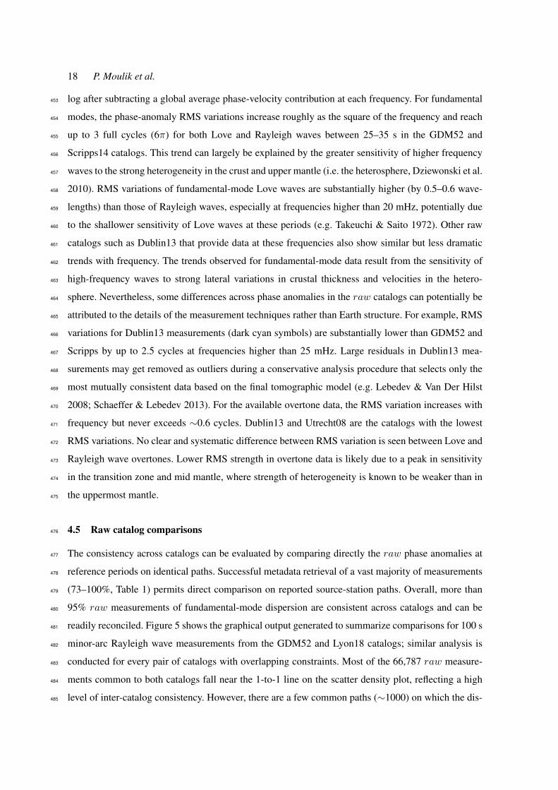
Figure 4 shows the root-mean-square (RMS) strength of the phase anomalies in the raw cata-452
18 P. Moulik et al.
log after subtracting a global average phase-velocity contribution at each frequency. For fundamental453
modes, the phase-anomaly RMS variations increase roughly as the square of the frequency and reach454
up to 3 full cycles (6π) for both Love and Rayleigh waves between 25–35 s in the GDM52 and455
Scripps14 catalogs. This trend can largely be explained by the greater sensitivity of higher frequency456
waves to the strong heterogeneity in the crust and upper mantle (i.e. the heterosphere, Dziewonski et al.457
2010). RMS variations of fundamental-mode Love waves are substantially higher (by 0.5–0.6 wave-458
lengths) than those of Rayleigh waves, especially at frequencies higher than 20 mHz, potentially due459
to the shallower sensitivity of Love waves at these periods (e.g. Takeuchi & Saito 1972). Other raw460
catalogs such as Dublin13 that provide data at these frequencies also show similar but less dramatic461
trends with frequency. The trends observed for fundamental-mode data result from the sensitivity of462
high-frequency waves to strong lateral variations in crustal thickness and velocities in the hetero-463
sphere. Nevertheless, some differences across phase anomalies in the raw catalogs can potentially be464
attributed to the details of the measurement techniques rather than Earth structure. For example, RMS465
variations for Dublin13 measurements (dark cyan symbols) are substantially lower than GDM52 and466
Scripps by up to 2.5 cycles at frequencies higher than 25 mHz. Large residuals in Dublin13 mea-467
surements may get removed as outliers during a conservative analysis procedure that selects only the468
most mutually consistent data based on the final tomographic model (e.g. Lebedev & Van Der Hilst469
2008; Schaeffer & Lebedev 2013). For the available overtone data, the RMS variation increases with470
frequency but never exceeds ∼0.6 cycles. Dublin13 and Utrecht08 are the catalogs with the lowest471
RMS variations. No clear and systematic difference between RMS variation is seen between Love and472
Rayleigh wave overtones. Lower RMS strength in overtone data is likely due to a peak in sensitivity473
in the transition zone and mid mantle, where strength of heterogeneity is known to be weaker than in474
the uppermost mantle.475
4.5 Raw catalog comparisons476
The consistency across catalogs can be evaluated by comparing directly the raw phase anomalies at477
reference periods on identical paths. Successful metadata retrieval of a vast majority of measurements478
(73–100%, Table 1) permits direct comparison on reported source-station paths. Overall, more than479
95% raw measurements of fundamental-mode dispersion are consistent across catalogs and can be480
readily reconciled. Figure 5 shows the graphical output generated to summarize comparisons for 100 s481
minor-arc Rayleigh wave measurements from the GDM52 and Lyon18 catalogs; similar analysis is482
conducted for every pair of catalogs with overlapping constraints. Most of the 66,787 raw measure-483
ments common to both catalogs fall near the 1-to-1 line on the scatter density plot, reflecting a high484
level of inter-catalog consistency. However, there are a few common paths (∼1000) on which the dis-485

Global Reference Seismological Datasets: Surface Waves 19
crepancies between catalogs are large (≥ π/4 radians). Most of these paths correspond to full-cycle486
differences in phase (±2π), which can be a cycle-skipping issue in either catalog. Moreover, GDM52487
reports slower velocities with arrival times that are 1.4 s longer on average than Lyon18. Both mean488
and median absolute differences between the two catalogs binned every 2 show a steady increase with489
great-circle distance. These variations may be due to methodological assumptions, such as differences490
in the dispersion correction, geodetic constants or attenuation in the reference Earth model.491
Figures 6, S2–S13 summarize the catalog scatter comparisons for minor- and major-arc waves at492
50, 150 and 250 s. Mean differences in minor-arc data are usually low (< 2.54 s for R1 and L1 at 50 s)493
and rarely exceed π/4 radians for data between 25–250 s. Constraints on major-arc data afforded by494
MBS11 and GDM52 catalogs are also highly consistent with very low mean differences (<1.72 s) for495
150–250 s data. While the level of agreement between catalogs is generally high, some inconsistencies496
are seen across a wide band of frequencies. Full-cycle differences likely related to cycle-skipping497
issues are observed for 50 s waves between several pairs of catalogs (e.g. Lyon18–GDM52) and are498
more evident in minor-arc Rayleigh-wave data. Cycle skipping problems are more acute at shorter499
periods where it is harder to resolve the ambiguity in the number of cycles (Section 3). Such issues500
are also noted for station pairs at large epicentral distances along strongly heterogeneous paths for501
which the accrued phase delay may approach or exceed the period. The use of GDM52 as the starting502
model in Scripps14 helps alleviate some of the cycle-skipping issues (Section 4.2), producing greater503
overall consistency between the two catalogs. Much of the scatter in several catalog-pairs are from504
measurements at epicentral distances outside the distance range 30–150 used in the construction of505
the reference dataset.506
In the interest of brevity, we summarize the agreement for all types of fundamental-mode measure-507
ments in Figure 7. For every pair of catalogs, median absolute deviations in reported measurements508
of Love and Rayleigh waves are plotted against reference period. Median differences in fundamental-509
mode Love waves are uniformly low (<5 s) for all combinations of catalogs except for Cambridge19510
where discrepancies with GDM52, MBS11 and Scripps14 can exceed 6 s at the longest periods511
(>150 s). In contrast, consistency deteriorates for Rayleigh waves with median absolute differences512
exceeding 6 s for some pairs of catalogs (e.g. Cambridge19-Scripps14) at the longest periods (> 200 s).513
Dublin13 and Utrecht08 have the most consistent Love- and Rayleigh-wave measurements with me-514
dian differences not exceeding 1.5 s across 40–150 s period band. This reflects the central role that515
automated multimode inversion (Lebedev et al. 2005) plays in both catalogs (Visser & Trampert 2008).516
Median values for Rayleigh waves binned every 2 in epicentral distance show a clear deterioration in517
agreement outside the distance range 30–150.518
Despite the low median differences between raw catalogs, our comparisons reveal a systematic519
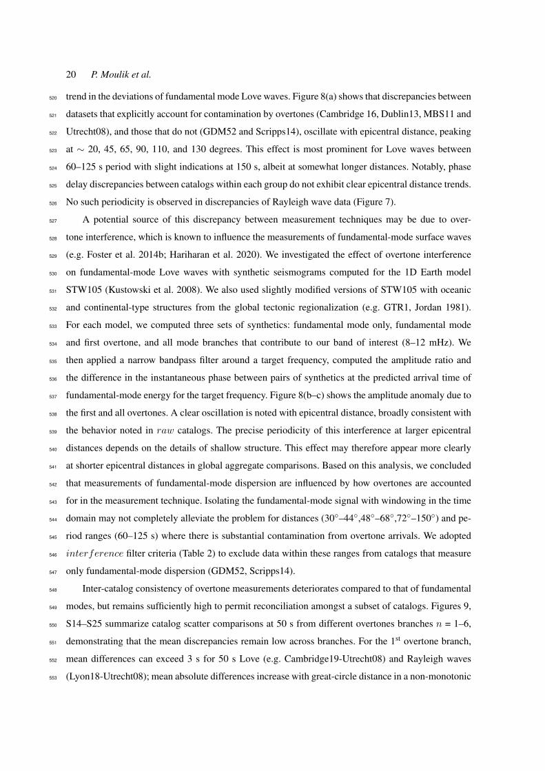
20 P. Moulik et al.
trend in the deviations of fundamental mode Love waves. Figure 8(a) shows that discrepancies between520
datasets that explicitly account for contamination by overtones (Cambridge 16, Dublin13, MBS11 and521
Utrecht08), and those that do not (GDM52 and Scripps14), oscillate with epicentral distance, peaking522
at ∼ 20, 45, 65, 90, 110, and 130 degrees. This effect is most prominent for Love waves between523
60–125 s period with slight indications at 150 s, albeit at somewhat longer distances. Notably, phase524
delay discrepancies between catalogs within each group do not exhibit clear epicentral distance trends.525
No such periodicity is observed in discrepancies of Rayleigh wave data (Figure 7).526
A potential source of this discrepancy between measurement techniques may be due to over-527
tone interference, which is known to influence the measurements of fundamental-mode surface waves528
(e.g. Foster et al. 2014b; Hariharan et al. 2020). We investigated the effect of overtone interference529
on fundamental-mode Love waves with synthetic seismograms computed for the 1D Earth model530
STW105 (Kustowski et al. 2008). We also used slightly modified versions of STW105 with oceanic531
and continental-type structures from the global tectonic regionalization (e.g. GTR1, Jordan 1981).532
For each model, we computed three sets of synthetics: fundamental mode only, fundamental mode533
and first overtone, and all mode branches that contribute to our band of interest (8–12 mHz). We534
then applied a narrow bandpass filter around a target frequency, computed the amplitude ratio and535
the difference in the instantaneous phase between pairs of synthetics at the predicted arrival time of536
fundamental-mode energy for the target frequency. Figure 8(b–c) shows the amplitude anomaly due to537
the first and all overtones. A clear oscillation is noted with epicentral distance, broadly consistent with538
the behavior noted in raw catalogs. The precise periodicity of this interference at larger epicentral539
distances depends on the details of shallow structure. This effect may therefore appear more clearly540
at shorter epicentral distances in global aggregate comparisons. Based on this analysis, we concluded541
that measurements of fundamental-mode dispersion are influenced by how overtones are accounted542
for in the measurement technique. Isolating the fundamental-mode signal with windowing in the time543
domain may not completely alleviate the problem for distances (30–44,48–68,72–150) and pe-544
riod ranges (60–125 s) where there is substantial contamination from overtone arrivals. We adopted545
interference filter criteria (Table 2) to exclude data within these ranges from catalogs that measure546
only fundamental-mode dispersion (GDM52, Scripps14).547
Inter-catalog consistency of overtone measurements deteriorates compared to that of fundamental548
modes, but remains sufficiently high to permit reconciliation amongst a subset of catalogs. Figures 9,549
S14–S25 summarize catalog scatter comparisons at 50 s from different overtones branches n = 1–6,550
demonstrating that the mean discrepancies remain low across branches. For the 1st overtone branch,551
mean differences can exceed 3 s for 50 s Love (e.g. Cambridge19-Utrecht08) and Rayleigh waves552
(Lyon18-Utrecht08); mean absolute differences increase with great-circle distance in a non-monotonic553
Global Reference Seismological Datasets: Surface Waves 21
fashion reaching∼8 s at 120. Comparisons for higher overtone branches reveal a similarly high level554
of agreement (e.g. 50 s Dublin13-Utrecht08) and a clear trend with epicentral distance, although fewer555
common measurements are available. The median absolute differences in phase anomalies from vari-556
ous catalogs show a less clear trend as a function of period for 1st and 2nd overtone branches (Figure 10)557
than is observed for the fundamental modes. Overall, the discrepancies across overtone branches 1–6558
are uniformly low (<5 s) for the period bands specified in Table 2. Utrecht08 and Dublin13 catalogs559
show consistently higher levels of agreement than other catalogs across all mode branches except the560
first overtone. Discrepancies increase with great-circle distance for all combinations of catalogs with561
no clear relation to the overtone branch, indicating differences in the reference 1D Earth models or562
geodetic constants.563
5 REFERENCE DATASET564
Construction of a reference dataset includes calculation of summary rays and removal of outliers565
for clean catalogs. These analyses provide further insights into the sources and estimates of uncer-566
tainties in the reported measurements.567
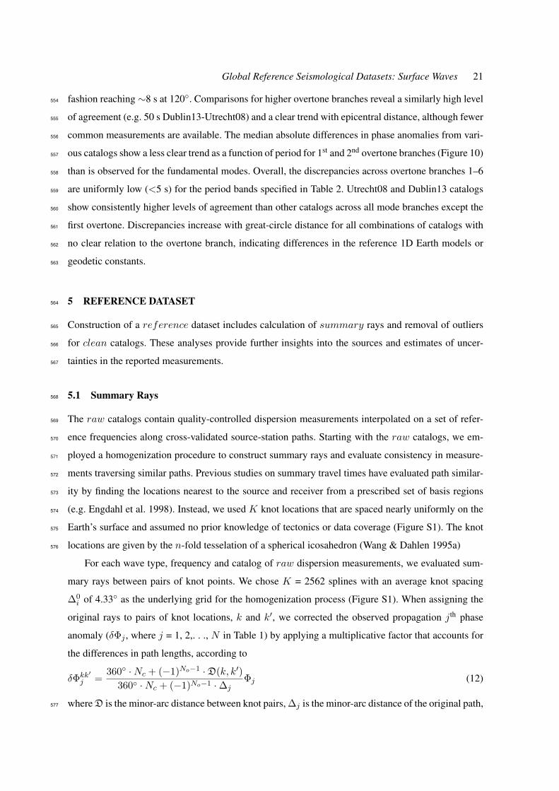
5.1 Summary Rays568
The raw catalogs contain quality-controlled dispersion measurements interpolated on a set of refer-569
ence frequencies along cross-validated source-station paths. Starting with the raw catalogs, we em-570
ployed a homogenization procedure to construct summary rays and evaluate consistency in measure-571
ments traversing similar paths. Previous studies on summary travel times have evaluated path similar-572
ity by finding the locations nearest to the source and receiver from a prescribed set of basis regions573
(e.g. Engdahl et al. 1998). Instead, we used K knot locations that are spaced nearly uniformly on the574
Earth’s surface and assumed no prior knowledge of tectonics or data coverage (Figure S1). The knot575
locations are given by the n-fold tesselation of a spherical icosahedron (Wang & Dahlen 1995a)576
For each wave type, frequency and catalog of raw dispersion measurements, we evaluated sum-
mary rays between pairs of knot points. We chose K = 2562 splines with an average knot spacing
∆0i of 4.33 as the underlying grid for the homogenization process (Figure S1). When assigning the
original rays to pairs of knot locations, k and k′, we corrected the observed propagation jth phase
anomaly (δΦj , where j = 1, 2,. . ., N in Table 1) by applying a multiplicative factor that accounts for
the differences in path lengths, according to
δΦkk′j =
360 ·Nc + (−1)No−1 ·D(k, k′)
360 ·Nc + (−1)No−1 ·∆jΦj (12)
where D is the minor-arc distance between knot pairs, ∆j is the minor-arc distance of the original path,577
22 P. Moulik et al.
No the orbit number and Nc is the number of times circled around the Earth. The correction factor578
above accounts for the total distance traversed by the wave and is therefore larger for higher-orbits579
waves (R3–R5, L3–L5). We excluded subsets of catalogs when none of the knot pairs satisfied the580
minimum number of two contributing original paths e.g. Rayleigh wave overtone data from Dublin13581
(2nd Over. : 250–350s; 3rd Over. : 250–300s, 4th Over. : 150–200s) and MBS11 catalogs (2nd Over.582
: 250s, 4th Over. : 75s). Homogenized data and deviations/uncertainties across all knot pairs (k,k′)583
are defined, respectively, as the mean and standard deviation of all associated corrected measurements584
(Φkk′j ).585
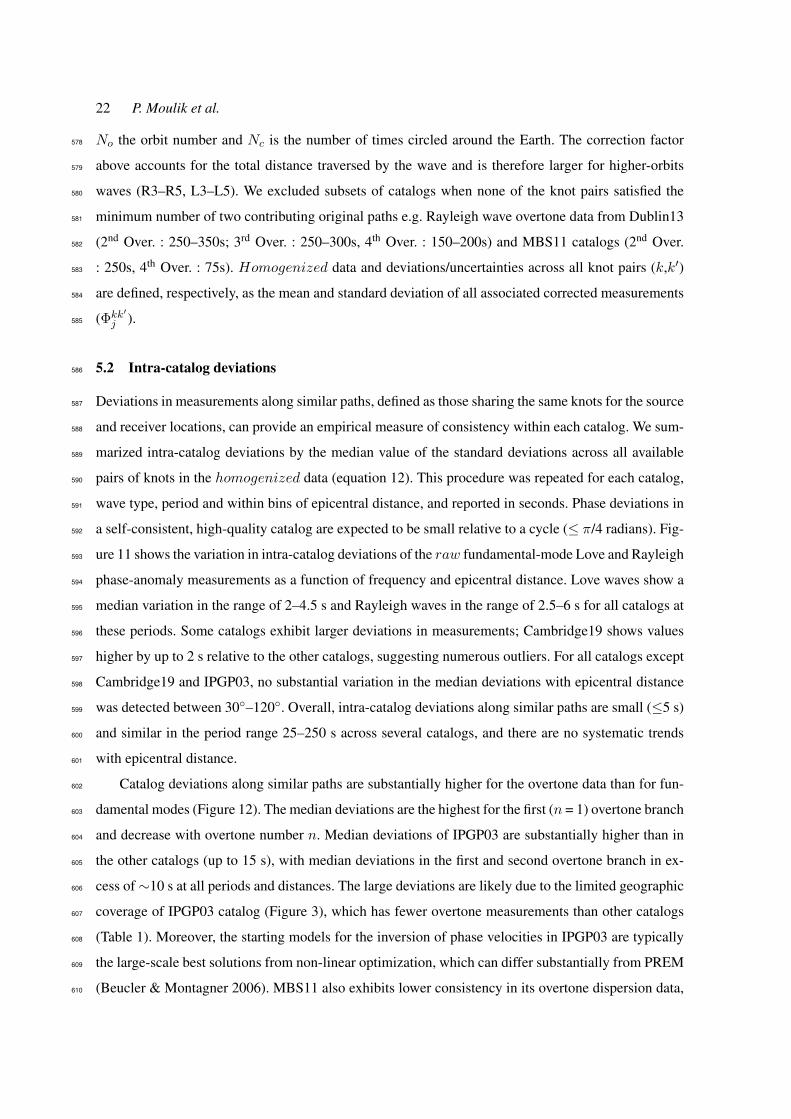
5.2 Intra-catalog deviations586
Deviations in measurements along similar paths, defined as those sharing the same knots for the source587
and receiver locations, can provide an empirical measure of consistency within each catalog. We sum-588
marized intra-catalog deviations by the median value of the standard deviations across all available589
pairs of knots in the homogenized data (equation 12). This procedure was repeated for each catalog,590
wave type, period and within bins of epicentral distance, and reported in seconds. Phase deviations in591
a self-consistent, high-quality catalog are expected to be small relative to a cycle (≤ π/4 radians). Fig-592
ure 11 shows the variation in intra-catalog deviations of the raw fundamental-mode Love and Rayleigh593
phase-anomaly measurements as a function of frequency and epicentral distance. Love waves show a594
median variation in the range of 2–4.5 s and Rayleigh waves in the range of 2.5–6 s for all catalogs at595
these periods. Some catalogs exhibit larger deviations in measurements; Cambridge19 shows values596
higher by up to 2 s relative to the other catalogs, suggesting numerous outliers. For all catalogs except597
Cambridge19 and IPGP03, no substantial variation in the median deviations with epicentral distance598
was detected between 30–120. Overall, intra-catalog deviations along similar paths are small (≤5 s)599
and similar in the period range 25–250 s across several catalogs, and there are no systematic trends600
with epicentral distance.601
Catalog deviations along similar paths are substantially higher for the overtone data than for fun-602
damental modes (Figure 12). The median deviations are the highest for the first (n = 1) overtone branch603
and decrease with overtone number n. Median deviations of IPGP03 are substantially higher than in604
the other catalogs (up to 15 s), with median deviations in the first and second overtone branch in ex-605
cess of∼10 s at all periods and distances. The large deviations are likely due to the limited geographic606
coverage of IPGP03 catalog (Figure 3), which has fewer overtone measurements than other catalogs607
(Table 1). Moreover, the starting models for the inversion of phase velocities in IPGP03 are typically608
the large-scale best solutions from non-linear optimization, which can differ substantially from PREM609
(Beucler & Montagner 2006). MBS11 also exhibits lower consistency in its overtone dispersion data,610
Global Reference Seismological Datasets: Surface Waves 23
with median deviations similar to IPGP03 for the first overtone branch (∼5–10 s). The overlapping611
measurement periods cover a narrower period band for the third and higher overtone branch (50–60 s),612
where the median deviations are also uniformly low (±5 s) for all catalogs except the IPGP03 cata-613
log. Except for Lyon18 and Cambridge19, none of the larger catalogs show a clear trend of median614
deviation with great-circle distance for overtones in agreement with the fundamental-mode data.615
5.3 Outlier analysis616
Outlier identification and removal is critical to ensuring consistency across catalogs and robustness617
of phase-slowness inversions. It is particularly important to assess the relative quality of the mea-618
surements and flag inconsistencies because (semi)automated methods can be improved by our filter619
criteria. While these methods enable fast data processing and generation of large sets of dispersion620
data, they lack the detailed oversight of a domain expert inherent in fully-supervised techniques. We621
obtained a clean dataset on original paths and an associated clean homogenized dataset for each622
catalog after the removal of outliers. Our definition of an outlier is based on, (1) large intra-catalog623
deviations on similar paths, (2) clear half (±0.9–1.1 · π) or full-cycle discrepancies (±0.9–1.1 · 2π) on624
original paths, (3) large inter-catalog inconsistencies on similar paths (|δφkk′2 -δφkk′
1 | > 0.4 · 2π), (4)625
quality criteria of distance and period ranges where the signal is most easily measured across tech-626
niques, (5) source depths and magnitudes where excitation is strongest, (4) criteria based on overtone627
interference (Section 4.5). Table 2 summarizes the configuration of some of these quality control628
criteria in our processing scheme.629
Because measurements associated to a knot pair (k, k′) correspond to very similar source-station630
paths, we excluded all knot pairs and contributing paths if the standard deviations exceeded 10 times631
the median of corrected phase anomalies (δΦkk′j , equation 12) across all catalogs. We adopted the632
median as the preferred value for catalog comparisons since it is less affected by outliers. Half- and633
full-cycle discrepancies indicating polarity reversals and cycle skips that were identified in Section 4.5634
were also excluded. Finally, we excluded the knot pairs and their contributing paths as outliers when635
there were large inconsistencies (>0.4 · 2π) between pairs of homogenized catalogs.636
Figure 13 shows the effect of quality-control criteria (Section 4.4) and the outlier analysis for637
100 s minor-arc Rayleigh wave measurements. Only a small fraction of paths (< 0.01%) from the638
contributed catalogs were excluded as outliers during the creation of the clean dataset. A substantial639
fraction (> 25%, pie chart) of the removed outliers in IPGP03 are due to intra-catalog inconsistencies640
while the bulk of outliers in other catalogs are due to source and quality filter criteria. A slight im-641
provement in consistency within catalogs is observed after the removal of outliers based on catalog642
median uncertainties. Inter-quartile ranges of homogenized phase anomalies and uncertainties also de-643

24 P. Moulik et al.
crease from raw to clean catalogs. Since a limited number of original paths are removed between the644
two catalogs, median deviations do not change substantially between the two catalogs. Removal of out-645
liers has a detectable effect on the RMS variations of phase anomalies in fundamental-mode Rayleigh646
waves, though the values remain similar to within ±0.5 radians (Figure 4). The RMS variation in the647
clean catalog at periods shorter than 35 s increases by up to ∼1 wavelength in case of Dublin13 data,648
which has the desirable effect of improving its consistency with GDM52 and Scripps14 catalogs. This649
is due to the substantial number of short paths with small phase anomalies in the Dublin13 catalog,650
which gets removed during our procedure (Table 2).651
Analysis of outliers provides interesting insights on the waveforms from which the measurements652
were derived. For example, half-cycle discrepancies (π) between GDM52 and Scripps14 catalogs653
at some periods (Figure 14, 100 s) are typically associated with specific stations. Geofon stations654
KSDI-GE, JER-GE and a few others (VSL-MN, AIS-G) show the most number of discrepancies (10–655
40 paths). Such outliers are likely due to reversed polarities of stations such as KSDI-GE and AIS-G in656
certain time periods, which may not be reflected in the instrument response history. The time history657
of potential reversals can be identified from the comparison of catalogs and the retrieved CMT source658
mechanism. We found some qualitative agreement between our list of possible polarity reversals and659
those employed in the processing of Scripps14 data. Automatic detection of reversed polarities may660
require accurate propagation phase predictions from a 3D reference Earth model.661
5.4 Summary data and uncertainties662
The large amounts of surface-wave measurements analyzed in this study presented a major com-663
putational burden. At the same time, both inter- and intra-catalog consistency suggests a level of664
redundancy in the contributed measurements that justifies constructing a summary dataset. First,665
neighboring modes within the same nth-overtone branch have very similar theoretical sensitivities to666
radial structure. Very fine sampling of the dispersion curve may not therefore provide independent667
structural constraints. Second, dispersion is often contributed in terms of propagation phase anoma-668
lies at arbitrarily sampled frequencies (Ncontrib, Table 1), which may not accurately represent the in-669
formation content in a catalog. Due to the approximations inherent to the measurement technique,670
Dublin13 provides finely sampled dispersion curves resulting in a very large number of contributed671
data (3–8 X Ncontrib, Table 1). However, the number of unique source-station paths (Npath) in Dublin13672
is comparable or even lower than in other recent catalogs (e.g. Scripps14, Cambridge19, MBS11,673
Lyon18).674
Our processing scheme results in a summary dataset that represents the best estimates and uncer-675
tainties of phase anomalies between knot pairs (Figure 2). Phase anomalies in the summary dataset676

Global Reference Seismological Datasets: Surface Waves 25
(δΦ) were calculated from the median estimates of all clean homogenized catalogs. The knot loca-677
tions (K = 2562) specified in the homogenization of raw and clean catalogs are therefore preserved in678
the summary catalogs. Our procedure also accounts for overlapping coverage from various catalogs679
and inter-catalog consistencies. Systematic inconsistencies due to geodetic constants and reference680
1D models were averaged out. All reference phases (Φ0P ) reported in the summary data were derived681
using updated geodetic constants (Section 4.3). Based on our experiments, such baseline issues do not682
influence substantially the lateral phase-velocity variations that are the focus of this study and most683
potential applications of the reference dataset.684
We estimated observational uncertainties of the phase anomalies empirically by comparing mea-685
surements for similar paths (Section 5.1). The knot pairs in the summary dataset were determined to686
be of quality A, B or C, depending on the number and consistency of independent constraints from687
various catalogs. If only a single clean catalog provided constraints, the knot pair was assigned the688
poorest C grade when a single source-station path was available, or a B grade when multiple paths689
were available with highly consistent measurements, i.e. phase anomaly deviations did not exceed the690
median of catalog uncertainties. When multiple clean catalogs provided constraints, knot pairs were691
assigned an A grade if they exhibited high levels of both intra- and inter-catalog consistency. The692
inter-catalog consistency was considered high if all catalogs had uncertainties within the 2-σ level of693
their median value. Due to the strict criteria adopted here, only a limited number of knot-pair paths in694
the summary dataset were assigned the A grade.695
Observed variations in the measured phase anomalies along similar paths reflect errors in the (1)696
source location, (2) CMT focal mechanism, (3) source excitation, due to incorrect source depth or local697
structure, (4) interference of the fundamental mode with overtones, (5) instrument-response correction,698
and (6) errors due to seismic noise. Figure 15 and Table 3 show the estimated uncertainty for the most699
numerous quality-B observations as a function of frequency, indicating a roughly linear increase in700
the phase uncertainty with increasing frequency. This trend is observed both in the summary catalog701
and the contributing clean catalogs, although some catalogs such as MBS11 and Utrecht08 tend to702
have steeper gradients. A linear increase in phase uncertainty with frequency is also found in the703
case of overtone catalogs (Table 3). These observations may be related to possible source mislocation704
of 16–25 km in the direction to or from the station (e.g. Smith & Ekstrom 1996; Ekstrom 2011). It705
is difficult to reliably disentangle the combined effects of the error sources, especially because the706
empirical uncertainty reported here may underestimate the true uncertainty of the measurements.707
26 P. Moulik et al.
6 IMPLICATIONS FOR EARTH STRUCTURE708
Robustness in the features of mantle heterogeneity may be assessed with the phase-velocity variations709
inverted from the clean and summary datasets. Outstanding questions include identifying redundan-710
cies in the raw catalogs and structural complexities that are largely independent of the measurement711
technique.712
6.1 Phase-velocity maps713
We wish to determine the two-dimensional (2D) variations in local phase slowness or velocity as
a function of co-latitude θ and longitude ϕ. Such phase-velocity maps are optimized to fit a set of
observed propagation phase anomalies at a given period, while accounting for azimuthal variations due
to anisotropy. In a weakly anisotropic Earth, azimuthal variations in Love and Rayleigh wave velocities
can be described by patterns with simple two-fold (2ζ) and four-fold (4ζ) azimuthal symmetry (Smith
& Dahlen 1973). Such variations are defined in terms of the propagation azimuth ζ with respect to the
local meridian, following
p?(ζ) = p0(1 +δp
p0+A cos 2ζ +B sin 2ζ + C cos 4ζ +D sin 4ζ), (13)
where p?(ζ) is the full, azimuthally varying, phase slowness and A, B, C, and D are coefficients714
describing azimuthal variations in phase slowness with respect to the reference isotropic slowness p0.715
We can invert for lateral variations in anisotropic properties,716
δp?(θ, ϕ; ζ)
p0=
δp(θ, ϕ)
p0+A(θ, ϕ) cos 2ζ +B(θ, ϕ) sin 2ζ +
C(θ, ϕ) cos 4ζ +D(θ, ϕ) sin 4ζ. (14)
where laterally varying coefficients A(θ, ϕ), B(θ, ϕ), C(θ, ϕ), and D(θ, ϕ) are expanded in terms of
a finite set of basis functions fi(θ, ϕ) on the surface of the sphere, for example
A(θ, ϕ) =K∑i=1
aifi(θ, ϕ), (15)
where ai are the model coefficients, andK is the total number of basis functions used in this represen-
tation. Since local phase slowness perturbations (δp/p0) in the period range analyzed in this paper can
be larger than 20%, we avoid the approximation1/(1 + δc/c0) ≈ 1− δc/c0, which is commonly used
to linearize the tomographic problem for small perturbations δc(θ, ϕ) in local phase velocity. When
the results below are discussed in terms of velocity variations, (δc/c0), these variations are calculated
from the slowness variations by
δc
c0=−δp
p0 + δp. (16)
Global Reference Seismological Datasets: Surface Waves 27
In order to represent a smoothly varying direction of azimuthal variations in regions close to the poles,717
we reference the changing azimuth along a raypath to the ‘local parallel azimuth’ of a parallel line718
passing through the nearest spline knot location (Ekstrom 2006a).719
As our set of basis functions, we choose spherical splines defined on an equispaced set of knot
locations, given by the n-fold tesselation of a spherical icosahedron (Wang & Dahlen 1995a). The i-th
basis function fi(θ, φ) depends on the distance ∆ from the i-th knot point as follows:
fi =
34(∆/∆0
i )3 − 3
2(∆/∆0i )
2 + 1, ∆ ≤ ∆0i
−14(∆/∆0
i )3 + 3
2(∆/∆0i )
2 − 3(∆/∆0i ) + 2, ∆0
i ≤ ∆ ≤ 2∆0i ,
(17)
where 2∆0i is the full range of the i-th spline basis function, and ∆0
i is set equal to the average distance720
between knot points. Specifically, we adopt a basis set containing K = 1442 splines with an average721
knot spacing ∆0i of 5.77 (Figure S1).722
Starting from equation 9, we obtain a set of linear equations to predict the N number of observed723
phase anomalies for each period and wave type [δΦobs.j ; j=1,2,...,N ]. These observations are related to724
the local slowness variations described by the set of spherical spline coefficients as725
δΦobs.j =
∑i
∫jfi(θ, φ) [pi + ai cos(2ζ) + bi sin(2ζ) + ci cos(4ζ) + di sin(4ζ)] ds. (18)
Here, the integration is performed over the source-station path θj ,φj corresponding to the jth ob-726
servation, summation is over all non-zero splines along the path, and pi are the coefficients of the727
isotropic part of the model.728
Based on prior studies of azimuthal anisotropy variations (Ekstrom 2011; Ma et al. 2014) and729
on expectations from mineralogy (e.g. Montagner & Nataf 1986; Montagner & Anderson 1989), we730
restrict our inversion to the 2ζ terms (A and B) for Rayleigh waves, and the 4ζ terms (C and D) for731
Love waves. This imposes the same number of free parameters in the Love and Rayleigh inversions and732
facilitates evaluation of the appropriate level of model complexity. For Rayleigh waves, neglecting 4ζ733
variations has previously been shown to not substantially influence the retrieved maps of 2ζ variations734
(Maggi et al. 2006).735
The chi-squared misfit χ2 which is minimized in solving for optimal pi, ai, bi, ci, di is expressed
as:
χ2 =N∑j=1
w2j
σ2j
(δΦobs.
j − δΦpred.j
)2, (19)
where j is the index of the datum, σj is the observational uncertainty, δΦpred.j is the predicted phase736
anomaly for a given set of spline coefficients, and wj is a weight applied to the j-th observation.737
28 P. Moulik et al.
Weighting can be introduced to lower the contribution from highly-sampled paths or increase the
importance of paths important for coverage. To facilitate the use of data catalogs presented in this
study, we calculate the number of observations (NP ) that share the same starting and ending point on
2562 evenly distributed points (Section 5.1). Each observation corresponding to this path is assigned
an intra-catalog weight
wj = (1 + log10NP )−1, (20)
which down-weights the contribution to the χ2 from a path sampled repeatedly in a catalog (e.g. Ek-738
strom 2011), such as those from the active Tonga–Kermadec subduction zone (Figure 3, Section 4.1).739
Summary datasets on the evenly-spaced grid have more uniform coverage by construction; we there-740
fore set all weights to unity in inversions that utilize these data.741
Several corrections are often applied before interpreting the propagation phase anomalies in terms742
of interior structure. δΦref,ellip denotes correction due to different reference models and Earth’s hydro-743
static ellipticity, δΦζ represents the correction for azimuthal variations in surface-wave phase slow-744
ness, while δΦcrust is the correction due to the strong crustal heterogeneity (Table A1; Moulik &745
Ekstrom 2016, Appendix A). The corrected phase anomalies can then be attributed to variations in746
isotropic phase velocity (c) or slowness (p = 1/c) via equation 9. Our forward operator is linear, and747
the inverse problem can therefore be expressed as dobs = Gm, where G is the sensitivity matrix derived748
using GCRA. Since our objective here is not to infer Earth structure, but rather to obtain surface wave749
phase slowness maps, we ignore all structural corrections in the remainder of this study. The RSDF750
HDF5 container files include fields that store the data corrections (Table A1).751
Regularization is introduced to stabilize our inversion by minimizing the sum of χ2 and addi-
tional terms that quantify the amplitude or roughness of the phase slowness variations. We define the
isotropic roughness R as the RMS second-derivative gradient of the global isotropic phase-slowness
variations
R =
[1
4π
∫S
(∇2 δp
p0) · (∇2 δp
p0) dΩ
]1/2
. (21)
implemented by a discrete Laplacian on the knot points. Since the 1442 quasi-equispaced knot points
are constructed via dyadic subdivision of a spherical icosahedron (Figure S1), the discrete Laplacian
is evaluated for the 6 nearest neighbors of all but the 12 knots that have only 5 neighbors. We similarly
define the anisotropic roughnessesR2ζ andR4ζ as
Rnζ =
[1
4π
∫S
(∇2snζ) · (∇2snζ) + (∇2cnζ) · (∇2cnζ)
dΩ
]1/2
, (22)
where snζ and cnζ are the spatially varying sine and cosine coefficients of 2ζ and 4ζ anisotropy.
In a full inversion for isotropic, 2ζ and 4ζ-anisotropic phase-slowness variations, we then choose to
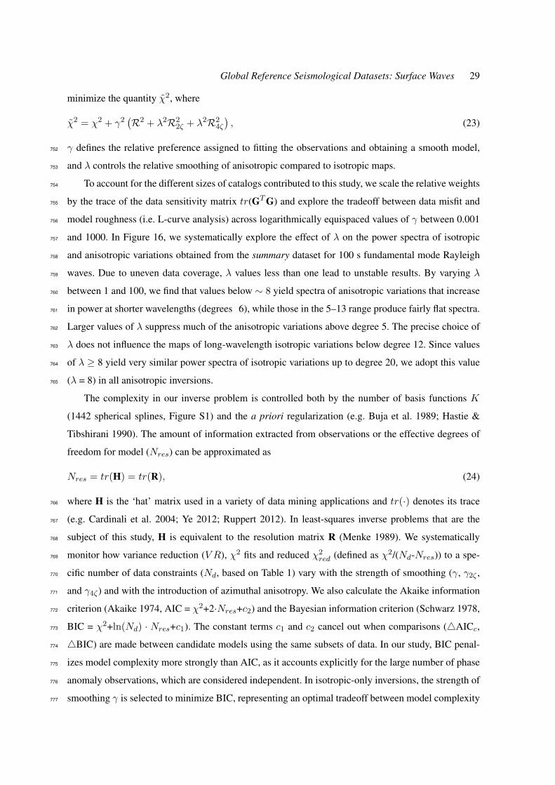
Global Reference Seismological Datasets: Surface Waves 29
minimize the quantity χ2, where
χ2 = χ2 + γ2(R2 + λ2R2
2ζ + λ2R24ζ
), (23)
γ defines the relative preference assigned to fitting the observations and obtaining a smooth model,752
and λ controls the relative smoothing of anisotropic compared to isotropic maps.753
To account for the different sizes of catalogs contributed to this study, we scale the relative weights754
by the trace of the data sensitivity matrix tr(GTG) and explore the tradeoff between data misfit and755
model roughness (i.e. L-curve analysis) across logarithmically equispaced values of γ between 0.001756
and 1000. In Figure 16, we systematically explore the effect of λ on the power spectra of isotropic757
and anisotropic variations obtained from the summary dataset for 100 s fundamental mode Rayleigh758
waves. Due to uneven data coverage, λ values less than one lead to unstable results. By varying λ759
between 1 and 100, we find that values below ∼ 8 yield spectra of anisotropic variations that increase760
in power at shorter wavelengths (degrees 6), while those in the 5–13 range produce fairly flat spectra.761
Larger values of λ suppress much of the anisotropic variations above degree 5. The precise choice of762
λ does not influence the maps of long-wavelength isotropic variations below degree 12. Since values763
of λ ≥ 8 yield very similar power spectra of isotropic variations up to degree 20, we adopt this value764
(λ = 8) in all anisotropic inversions.765
The complexity in our inverse problem is controlled both by the number of basis functions K
(1442 spherical splines, Figure S1) and the a priori regularization (e.g. Buja et al. 1989; Hastie &
Tibshirani 1990). The amount of information extracted from observations or the effective degrees of
freedom for model (Nres) can be approximated as
Nres = tr(H) = tr(R), (24)
where H is the ‘hat’ matrix used in a variety of data mining applications and tr(·) denotes its trace766
(e.g. Cardinali et al. 2004; Ye 2012; Ruppert 2012). In least-squares inverse problems that are the767
subject of this study, H is equivalent to the resolution matrix R (Menke 1989). We systematically768
monitor how variance reduction (V R), χ2 fits and reduced χ2red (defined as χ2/(Nd-Nres)) to a spe-769
cific number of data constraints (Nd, based on Table 1) vary with the strength of smoothing (γ, γ2ζ ,770
and γ4ζ) and with the introduction of azimuthal anisotropy. We also calculate the Akaike information771
criterion (Akaike 1974, AIC = χ2+2·Nres+c2) and the Bayesian information criterion (Schwarz 1978,772
BIC = χ2+ln(Nd) · Nres+c1). The constant terms c1 and c2 cancel out when comparisons (4AICc,773
4BIC) are made between candidate models using the same subsets of data. In our study, BIC penal-774
izes model complexity more strongly than AIC, as it accounts explicitly for the large number of phase775
anomaly observations, which are considered independent. In isotropic-only inversions, the strength of776
smoothing γ is selected to minimize BIC, representing an optimal tradeoff between model complexity777
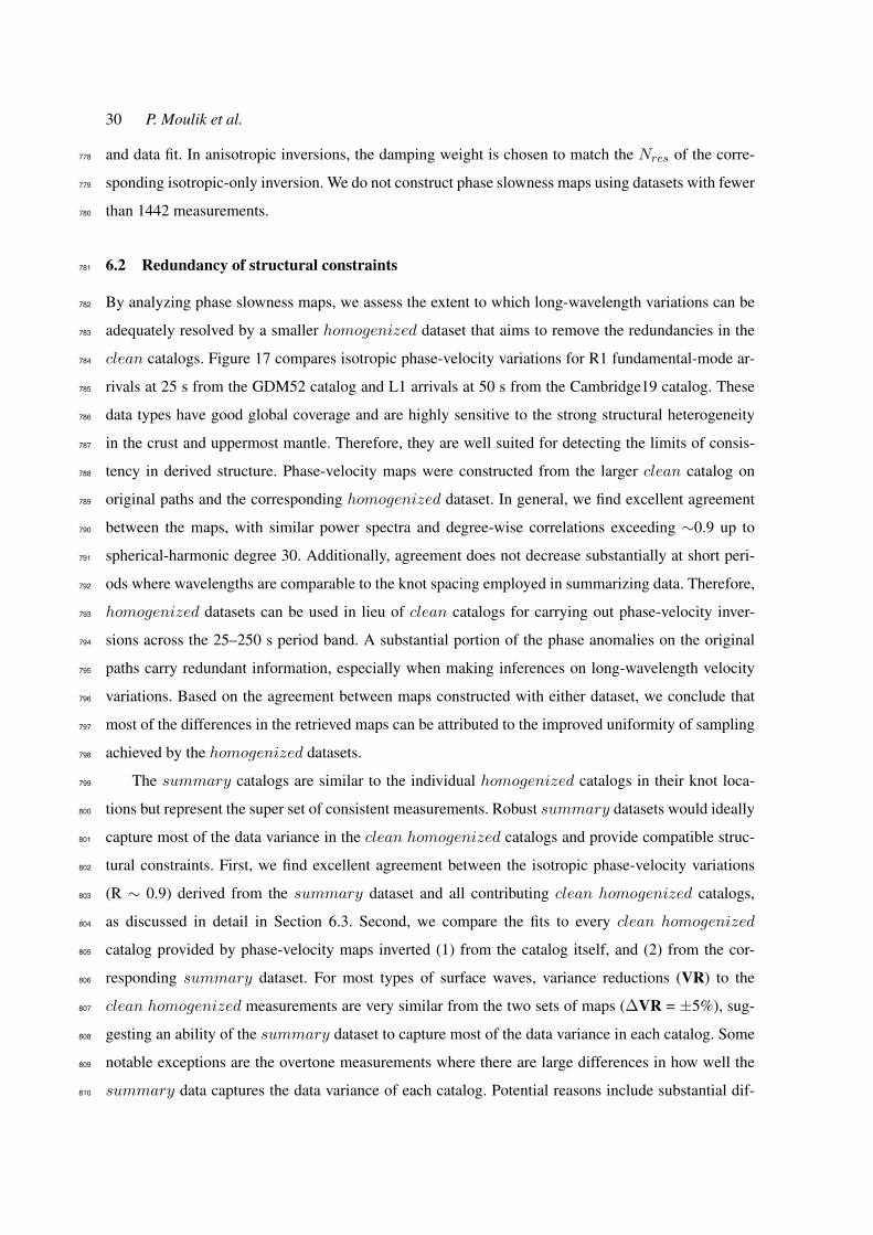
30 P. Moulik et al.
and data fit. In anisotropic inversions, the damping weight is chosen to match the Nres of the corre-778
sponding isotropic-only inversion. We do not construct phase slowness maps using datasets with fewer779
than 1442 measurements.780
6.2 Redundancy of structural constraints781
By analyzing phase slowness maps, we assess the extent to which long-wavelength variations can be782
adequately resolved by a smaller homogenized dataset that aims to remove the redundancies in the783
clean catalogs. Figure 17 compares isotropic phase-velocity variations for R1 fundamental-mode ar-784
rivals at 25 s from the GDM52 catalog and L1 arrivals at 50 s from the Cambridge19 catalog. These785
data types have good global coverage and are highly sensitive to the strong structural heterogeneity786
in the crust and uppermost mantle. Therefore, they are well suited for detecting the limits of consis-787
tency in derived structure. Phase-velocity maps were constructed from the larger clean catalog on788
original paths and the corresponding homogenized dataset. In general, we find excellent agreement789
between the maps, with similar power spectra and degree-wise correlations exceeding ∼0.9 up to790
spherical-harmonic degree 30. Additionally, agreement does not decrease substantially at short peri-791
ods where wavelengths are comparable to the knot spacing employed in summarizing data. Therefore,792
homogenized datasets can be used in lieu of clean catalogs for carrying out phase-velocity inver-793
sions across the 25–250 s period band. A substantial portion of the phase anomalies on the original794
paths carry redundant information, especially when making inferences on long-wavelength velocity795
variations. Based on the agreement between maps constructed with either dataset, we conclude that796
most of the differences in the retrieved maps can be attributed to the improved uniformity of sampling797
achieved by the homogenized datasets.798
The summary catalogs are similar to the individual homogenized catalogs in their knot loca-799
tions but represent the super set of consistent measurements. Robust summary datasets would ideally800
capture most of the data variance in the clean homogenized catalogs and provide compatible struc-801
tural constraints. First, we find excellent agreement between the isotropic phase-velocity variations802
(R ∼ 0.9) derived from the summary dataset and all contributing clean homogenized catalogs,803
as discussed in detail in Section 6.3. Second, we compare the fits to every clean homogenized804
catalog provided by phase-velocity maps inverted (1) from the catalog itself, and (2) from the cor-805
responding summary dataset. For most types of surface waves, variance reductions (VR) to the806
clean homogenized measurements are very similar from the two sets of maps (∆VR = ±5%), sug-807
gesting an ability of the summary dataset to capture most of the data variance in each catalog. Some808
notable exceptions are the overtone measurements where there are large differences in how well the809
summary data captures the data variance of each catalog. Potential reasons include substantial dif-810

Global Reference Seismological Datasets: Surface Waves 31
ferences in the geographical coverage among catalogs (e.g. IPGP versus MBS11) or other systematic811
inconsistencies in the measurements (Section 4.5).812
6.3 Consistency in isotropic heterogeneity813
In addition to the direct comparisons of phase anomaly measurements presented in Section 4.5, the814
degree of consistency across catalogs can be assessed by comparing the related inferences on interior815
structure. We constructed maps of (an)isotropic phase-velocity variations from the summary dataset816
of each type of surface wave. Figure 18 show isotropic phase-velocity variations in Love waves at817
100 s constructed using phase-anomaly measurements from the clean homogenized catalogs and the818
summary dataset. For Rayleigh waves, isotropic phase-velocity variations from anisotropic inver-819
sions are preferred (Figure 19 - right columns, Section 6.4). There is strong agreement between maps820
from various individual datasets, and the differences carry nearly indistinguishable structural implica-821
tions. The maps delineate shallow tectonic features as observed in upper mantle tomographic studies.822
Geological features in the Southern Hemisphere are more prominent when the homogenized data is823
employed in the inversion due to better coverage and uniform weighting of raypaths. For example, the824
fast cratonic features in Southern Africa are distinctly seen in Rayleigh wave maps constructed with825
every clean catalog and the summary dataset (Figure 19, right columns). Both the power of hetero-826
geneity and level of consistency are strongest at the longest wavelengths (degrees < 20). Moreover,827
data fit considerations also support the predominance of large-scale structure for the RMS variations828
in the catalogs. The RMS misfits to the homogenized data for degrees < 20 are within 10% of those829
corresponding to the full phase velocity map. Such large-scale features of global heterogeneity can830
adequately explain ∼90% of the signal in the phase delay measurements.831
In order to assess the level of consistency across length scales of heterogeneity, we compared832
the power spectra and degree-by-degree correlation between maps from various catalogs and the833
summary dataset. Reductions in correlations can result from inconsistencies in the measurements834
comprising each dataset or due to differences in coverage. Relatedly, differences in the power spec-835
tra can also reflect differences in the amount of smoothing that minimizes BIC for each catalog. We836
found that the agreement between phase-velocity variations persists for fundamental mode surface837
waves across all frequencies. Figure 20 shows the power spectra and degree-by-degree correlations of838
phase-velocity variations inferred for 50, 100 and 200 s Love and Rayleigh waves. For Love waves,839
high degree-by-degree correlations (R > 0.8) and similar power spectra across clean catalogs persist840
across degrees 1–15, degrading somewhat at the longest periods (200 s, L1). For Rayleigh waves,841
very high degree-by-degree correlations and similar power spectra persist across degrees 1–25 for842
most datasets, with the notable exception of IPGP03, whose small size tends to destabilize the re-843
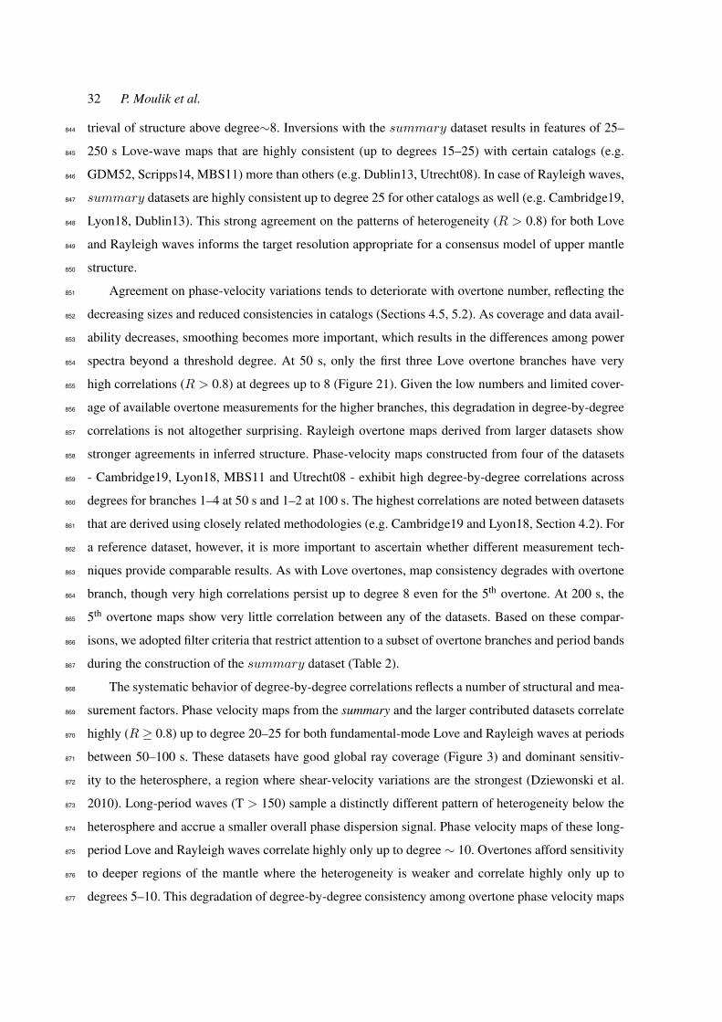
32 P. Moulik et al.
trieval of structure above degree∼8. Inversions with the summary dataset results in features of 25–844
250 s Love-wave maps that are highly consistent (up to degrees 15–25) with certain catalogs (e.g.845
GDM52, Scripps14, MBS11) more than others (e.g. Dublin13, Utrecht08). In case of Rayleigh waves,846
summary datasets are highly consistent up to degree 25 for other catalogs as well (e.g. Cambridge19,847
Lyon18, Dublin13). This strong agreement on the patterns of heterogeneity (R > 0.8) for both Love848
and Rayleigh waves informs the target resolution appropriate for a consensus model of upper mantle849
structure.850
Agreement on phase-velocity variations tends to deteriorate with overtone number, reflecting the851
decreasing sizes and reduced consistencies in catalogs (Sections 4.5, 5.2). As coverage and data avail-852
ability decreases, smoothing becomes more important, which results in the differences among power853
spectra beyond a threshold degree. At 50 s, only the first three Love overtone branches have very854
high correlations (R > 0.8) at degrees up to 8 (Figure 21). Given the low numbers and limited cover-855
age of available overtone measurements for the higher branches, this degradation in degree-by-degree856
correlations is not altogether surprising. Rayleigh overtone maps derived from larger datasets show857
stronger agreements in inferred structure. Phase-velocity maps constructed from four of the datasets858
- Cambridge19, Lyon18, MBS11 and Utrecht08 - exhibit high degree-by-degree correlations across859
degrees for branches 1–4 at 50 s and 1–2 at 100 s. The highest correlations are noted between datasets860
that are derived using closely related methodologies (e.g. Cambridge19 and Lyon18, Section 4.2). For861
a reference dataset, however, it is more important to ascertain whether different measurement tech-862
niques provide comparable results. As with Love overtones, map consistency degrades with overtone863
branch, though very high correlations persist up to degree 8 even for the 5th overtone. At 200 s, the864
5th overtone maps show very little correlation between any of the datasets. Based on these compar-865
isons, we adopted filter criteria that restrict attention to a subset of overtone branches and period bands866
during the construction of the summary dataset (Table 2).867
The systematic behavior of degree-by-degree correlations reflects a number of structural and mea-868
surement factors. Phase velocity maps from the summary and the larger contributed datasets correlate869
highly (R ≥ 0.8) up to degree 20–25 for both fundamental-mode Love and Rayleigh waves at periods870
between 50–100 s. These datasets have good global ray coverage (Figure 3) and dominant sensitiv-871
ity to the heterosphere, a region where shear-velocity variations are the strongest (Dziewonski et al.872
2010). Long-period waves (T > 150) sample a distinctly different pattern of heterogeneity below the873
heterosphere and accrue a smaller overall phase dispersion signal. Phase velocity maps of these long-874
period Love and Rayleigh waves correlate highly only up to degree ∼ 10. Overtones afford sensitivity875
to deeper regions of the mantle where the heterogeneity is weaker and correlate highly only up to876
degrees 5–10. This degradation of degree-by-degree consistency among overtone phase velocity maps877
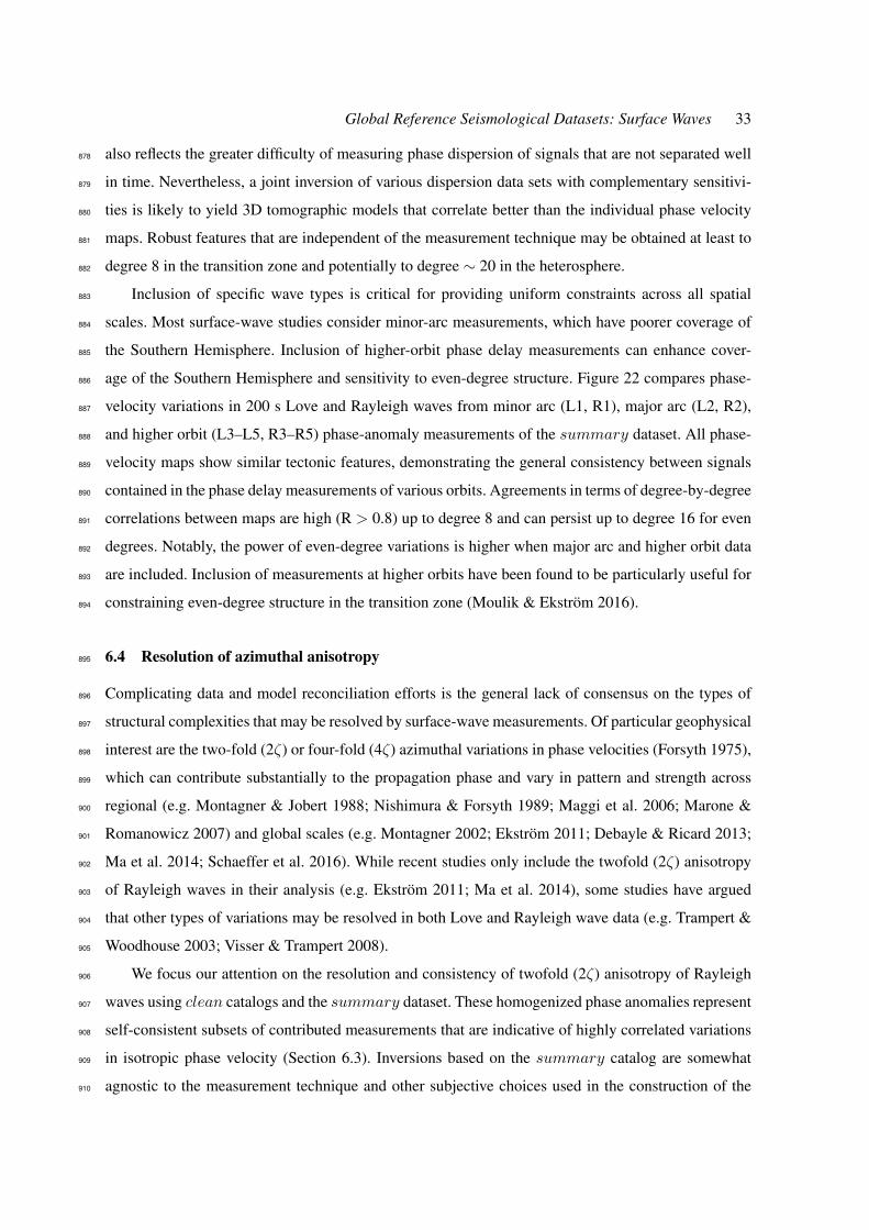
Global Reference Seismological Datasets: Surface Waves 33
also reflects the greater difficulty of measuring phase dispersion of signals that are not separated well878
in time. Nevertheless, a joint inversion of various dispersion data sets with complementary sensitivi-879
ties is likely to yield 3D tomographic models that correlate better than the individual phase velocity880
maps. Robust features that are independent of the measurement technique may be obtained at least to881
degree 8 in the transition zone and potentially to degree ∼ 20 in the heterosphere.882
Inclusion of specific wave types is critical for providing uniform constraints across all spatial883
scales. Most surface-wave studies consider minor-arc measurements, which have poorer coverage of884
the Southern Hemisphere. Inclusion of higher-orbit phase delay measurements can enhance cover-885
age of the Southern Hemisphere and sensitivity to even-degree structure. Figure 22 compares phase-886
velocity variations in 200 s Love and Rayleigh waves from minor arc (L1, R1), major arc (L2, R2),887
and higher orbit (L3–L5, R3–R5) phase-anomaly measurements of the summary dataset. All phase-888
velocity maps show similar tectonic features, demonstrating the general consistency between signals889
contained in the phase delay measurements of various orbits. Agreements in terms of degree-by-degree890
correlations between maps are high (R > 0.8) up to degree 8 and can persist up to degree 16 for even891
degrees. Notably, the power of even-degree variations is higher when major arc and higher orbit data892
are included. Inclusion of measurements at higher orbits have been found to be particularly useful for893
constraining even-degree structure in the transition zone (Moulik & Ekstrom 2016).894
6.4 Resolution of azimuthal anisotropy895
Complicating data and model reconciliation efforts is the general lack of consensus on the types of896
structural complexities that may be resolved by surface-wave measurements. Of particular geophysical897
interest are the two-fold (2ζ) or four-fold (4ζ) azimuthal variations in phase velocities (Forsyth 1975),898
which can contribute substantially to the propagation phase and vary in pattern and strength across899
regional (e.g. Montagner & Jobert 1988; Nishimura & Forsyth 1989; Maggi et al. 2006; Marone &900
Romanowicz 2007) and global scales (e.g. Montagner 2002; Ekstrom 2011; Debayle & Ricard 2013;901
Ma et al. 2014; Schaeffer et al. 2016). While recent studies only include the twofold (2ζ) anisotropy902
of Rayleigh waves in their analysis (e.g. Ekstrom 2011; Ma et al. 2014), some studies have argued903
that other types of variations may be resolved in both Love and Rayleigh wave data (e.g. Trampert &904
Woodhouse 2003; Visser & Trampert 2008).905
We focus our attention on the resolution and consistency of twofold (2ζ) anisotropy of Rayleigh906
waves using clean catalogs and the summary dataset. These homogenized phase anomalies represent907
self-consistent subsets of contributed measurements that are indicative of highly correlated variations908
in isotropic phase velocity (Section 6.3). Inversions based on the summary catalog are somewhat909
agnostic to the measurement technique and other subjective choices used in the construction of the910
34 P. Moulik et al.
contributed datasets. We evaluate the patterns of azimuthal anisotropy obtained with joint inversions911
of isotropic phase-velocity variations. Direct comparisons of isotropic and anisotropic inversions, how-912
ever, are made difficult by the compounding effects of regularization and parametrization.913
Regularization through smoothing of the phase-velocity variations is necessary to stabilize the914
inversion. Smoothing may not always be justified based on geological considerations (e.g. strong915
chemical boundaries), but is often necessary when the total number of model parameter is large (e.g.916
including anisotropic terms). The imposed smoothing complicates the direct comparison of isotropic-917
only and joint anisotropic inversions; changes in data fits cannot be attributed directly to an actual918
signal of anisotropy or to differences in regularization. As the strength of smoothing increases, the919
effective number of model parameters decreases and the data fits degrade monotonically. We enabled920
a direct comparison of data fits of the isotropic-only and joint anisotropic inversions through the fol-921
lowing procedure. First, we objectively chose an ‘optimal’ amount of smoothing (i.e. value of γ) for922
the isotropic-only inversion that minimized BIC, which represents an optimal tradeoff between model923
complexity and fit to data. Then, we systematically searched for the value of γ to be applied to the joint924
anisotropic inversion in order to produce a model with approximately the same number of resolved925
model parameters, Nres. Because the number of resolved model parameters does not exactly match,926
we compared data fits using the reduced χ2red statistic, which partially accounts for the changing num-927
ber of free parameters in the inversion (Nd - Nres).928
Figure 23 shows the fast axes and strengths of 2ζ anisotropy in 100 s fundamental-mode Rayleigh929
waves from clean catalogs and summary datasets. The magnitude and direction of fast axes are in930
good agreement between various recent catalogs. Qualitatively, the inversion results from this exper-931
iment are similar to those of previous studies (e.g. Trampert & Woodhouse 2003; Ekstrom 2011; Ma932
et al. 2014). Prominent large-scale features include east-west fast axes in the central Pacific Ocean933
and the weakest anisotropy across Eurasia. Only the relatively small IPGP03 catalog has coverage934
and resolution that is inadequate to robustly constrain the anisotropic patterns. We also investigated935
potential tradeoffs between isotropic and anisotropic variations in phase velocity. Figure 19 shows936
phase-velocity variations determined from an isotropic-only inversion alongside those from a joint937
anisotropic inversion of 100 s Rayleigh wave datasets. Isotropic phase-velocity variations are smoother938
in the joint inversions since they need to be described by fewer parameters. The most notable feature in939
the isotropic-only maps is the short-wavelength ripple or streak crossing the Pacific from the northeast940
to the southwest. This ripple is a stable feature of all high-resolution isotropic inversions of Rayleigh941
waves between 50 and 100 s period from several clean catalogs (Utrecht08, Dublin13, and GDM52)942
and summary datasets. In joint anisotropic inversions, the isotropic velocity ripple disappears and943
the phase velocity anomalies display a smooth increase in the Pacific Ocean basic from east to west,944
Global Reference Seismological Datasets: Surface Waves 35
consistent with the pattern expected from increasing age and cooling of the lithosphere (Stein & Stein945
1992).946
An outstanding question is whether the additional model complexity of anisotropy variations may947
be justified based on data. The improvement in data fit resulting from the introduction of anisotropic948
terms in the inverse problem is shown in Table 4. The introduction of anisotropic terms reduced χ2red949
for 25–250 s fundamental mode Rayleigh waves and most strongly at 100 s period (∆χ2red > 0.5).950
The signal of anisotropy is therefore strong for these types of waves and an 2ζ anisotropic model can951
explain the observed data significantly better than an isotropic model of similar complexity. Addition952
of 4ζ azimuthal terms to inversions of Love waves and their overtones did not decrease the reduced953
χ2red at any frequency for models with similar numbers of resolved parameters. It is not clear based954
on current catalogs if azimuthal anisotropy can be reliably constrained from other wave types on the955
basis of data fit and parsimony arguments. For example, decreases in reduced χ2red fits attributable to956
the inclusion of anisotropy were less than 1% for all Love overtones at 50 s and 100 s period. In case957
of Rayleigh wave overtones, the reduced χ2red decreased less than 2% at 50 s period and only 2–3% at958
100 s period. Notably, the relatively large errors associated with the overtone reference datasets may959
mask the signal of anisotropy in the transition zone that has been advocated based on single dataset960
studies (e.g. Yuan & Beghein 2014). Recent and ongoing efforts may improve the fidelity of overtone961
measurements leading to improved resolution of azimuthal anisotropy from overtone measurements962
(e.g. Xu & Beghein 2019).963
7 CONCLUSIONS964
The main result of this study is a global reference dataset of multi-mode surface-wave dispersion965
analyzed in collaboration with members of the seismological community and archived in a scalable966
data format. Our procedure for summary datasets effectively reduces redundancy, homogenizes ge-967
ographic coverage, and averages out measurement, station and source errors (e.g. Pulliam & Stark968
1993). The reference dataset comprises phase delays and uncertainties of fundamental-mode Love969
and Rayleigh waves between 25–250 s and progressively narrower period bands for overtones up to970
the 6th branch. After accounting for modeling approximations and salvaging missing metadata, we971
demonstrate a high level of consistency across most contributed measurements. High quality of the972
fundamental-mode measurements is evidenced by their uniformly low deviations (< 5 s) along sim-973
ilar paths for all periods and epicentral distances. A few inconsistent outliers can be attributed to974
cycle skipping, station polarity issues or overtone interference at specific epicentral distances. While975
deviations are larger for overtones than for fundamental modes, they remain small compared to the976
wavelength (< π/4 radians) and show no systematic trend with epicentral distance. Despite complica-977

36 P. Moulik et al.
tions with measuring overtone dispersion, consistency in the types of waves considered here remains978
high enough to permit reconciliation. Empirical uncertainties of the summary dataset are low but in-979
crease systematically with frequency for all overtone branches. Future work on multi-mode dispersion980
will benefit from precise measurements at higher overtone branches across wider period bands.981
Future surface-wave studies may converge towards greater agreement if certain choices in various982
processing schemes are made consistent. Reconciliation of large catalogs from diverse measurement983
techniques suggest potential guidelines. Open data-sharing policies across seismic networks will per-984
mit even larger portions of measurements and metadata to be cross-validated (e.g. Cambridge19),985
thereby extending the geographic coverage of current catalogs and promoting reproducible research.986
Strong agreement is noted within and across catalogs derived using semi-automated or supervised987
techniques. Lack of quality control in largely automated methods make issues like cycle skipping988
difficult to remove (e.g. MBS11), resulting in phase anomalies that can sometimes be abnormally989
large compared to the wavelengths (> 10π). Baseline discrepancies between techniques may be eas-990
ily avoided or reconciled if, (a) detailed information such as source and station metadata are pre-991
served in scalable data formats (Appendix A), (b) standard geodetic constants and dispersion cor-992
rections from (an)elastic reference Earth models are used while calculating the propagation phase,993
and (c) both distance- and frequency-dependence of overtone interference are considered while ap-994
plying quality-control criteria. Multi-mode dispersion across overtone branches may be difficult to995
disentangle and measure at short epicentral distances where there is not enough separation in arrivals996
of different modes. Overtone interference in Love waves can extend to teleseismic distances, con-997
taminating fundamental-mode-only measurements (GDM52, Scripps14). Processing choices such as998
filtering and windowing may not be adequate for avoiding all interference issues (e.g. Ekstrom et al.999
1997); accounting for mode coupling across all branches may be needed for the calculation of syn-1000
thetic seismograms.1001
The reference dataset presented here represents the current consensus on the available observa-1002
tions of surface wave dispersion between pairs of locations on Earth. Other types of observations have1003
been reported based on the routine processing of surface-wave arrivals on arrays of three-component1004
broadband seismometers. The amplitudes (e.g. Selby & Woodhouse 2002; Dalton & Ekstrom 2006),1005
group velocities (e.g. Ritzwoller et al. 2002; Ma & Masters 2014), arrival angles and polarization (e.g.1006
Laske & Masters 1996; Foster et al. 2014a), and ratios between vertical and horizontal components1007
(ZH ratio), are all theoretically sensitive to fine-scale lateral variations (e.g. Larson et al. 1998; Tan-1008
imoto & Rivera 2008). Focusing and defocusing of rays due to lateral heterogeneity can influence1009
the amplitudes of surface waves (AF , e.g. Woodhouse & Wong 1986; Park 1987; Romanowicz 1987;1010
Wang & Dahlen 1994), and thereby help constrain phase-velocity variations. Amplitude measurements1011
Global Reference Seismological Datasets: Surface Waves 37
of fundamental-mode Rayleigh waves can also constrain lateral variations of shear wave attenuation1012
in the upper mantle (e.g. Romanowicz 1995; Gung et al. 2003; Dalton et al. 2008; Adenis et al. 2017;1013
Karaoglu & Romanowicz 2018). Such emerging methods of characterizing surface wave arrivals pro-1014
vide sensitivity complementary to that of the propagation phase, especially to constrain small-scale1015
elastic variations that are beyond the scope of the REM3D project. We focused on constructing a ref-1016
erence dataset of large and diverse catalogs of propagation phase anomalies currently available from1017
the community.1018
We adopt the centroid locations based on the Global CMT project and do not solve simultane-1019
ously for the earthquake hypocenters in our phase-velocity inversions. In case of inversions that utilize1020
surface waves in isolation, source relocations are typically small (<15 km) but can be substantial in1021
localized regions (e.g. Andes) and influence the patterns of azimuthal anisotropy in Rayleigh waves1022
(Ma & Masters 2015). The average error in centroid locations of the Global CMT catalog due to lateral1023
heterogeneity and the presence of noise is∼10 km (Hjorleifsdottir & Ekstrom 2010), which is unlikely1024
to influence the long-wavelength anisotropic patterns in our study. Such small errors in the centroid1025
locations may be due to the incorporation of longer periods, which are sensitive to different parts1026
of the Earth’s structure, and using the full waveform of three wave types (body, surface and mantle)1027
rather than using the first arriving body waves in isolation (e.g. Smith & Ekstrom 1996). A systematic1028
assessment of the tradeoffs between azimuthal anisotropy and centroid locations would require joint1029
source-structure inversions with multiple data types, which is beyond the scope of this study.1030
Propagation phase measurements from diverse catalogs of multi-mode surface-wave dispersion1031
imply similar large-scale variations in the Earth’s mantle. Lateral phase-velocity variations based1032
on summary datasets can explain most of the data variance in the much larger (10–1000 times)1033
clean catalogs along original paths. Features of heterogeneity derived from the clean catalogs and1034
summary dataset are highly correlated (R> 0.8) in their long-wavelength variations for both fundamental-1035
mode measurements (lmax = 15) and overtones (lmax = 8). Only the two-fold (2ζ) azimuthal variations1036
in fundamental-mode Rayleigh waves are mapped consistently across catalogs and improve signifi-1037
cantly the fits to the reference dataset. Inclusion of both major-arc (R2, L2) and higher-orbit arrivals1038
(R3–R5, L3–L5) improves constraints on the even-degree phase-velocity variations. Our inferences1039
on interior structure are based on the simplifying assumption that surface waves travel along the great1040
circle connecting the source and receiver; other theoretical formulations need to be evaluated in fu-1041
ture work. As the current consensus dataset of multi-mode surface-wave dispersion, this reference1042
seismological dataset will provide robust constraints on the 3D reference Earth model.1043
38 P. Moulik et al.
ACKNOWLEDGMENTS1044
This material is based on work supported by National Science Foundation Grant EAR-1345082 and1045
the David and Lucile Packard Foundation. The reference datasets of multi-mode dispersion and un-1046
certainties from this study are available from the webpage http://rem3d.org.1047
REFERENCES
Adenis, A., Debayle, E., & Ricard, Y., 2017. Seismic evidence for broad attenuation anomalies in the astheno-
sphere beneath the Pacific Ocean, Geophysical Journal International, 209, 1677–1698.
Agnew, D., Berger, J., Buland, R., Farrell, W., & Gilbert, F., 1976. International deployment of accelerome-
ters:a network for very long period seismology, in EOS Trans. Am. Geophys. Union, vol. 57, pp. 180–188.
Akaike, H., 1974. A new look at the statistical model identification, IEEE Transactions on Automatic Control,
19(6), 716–723.
Aki, K. & Richards, P. G., 1980. Quantitative Seismology: Theory and Methods, vol. 2, W. H. Freeman and
Co, New York.
Beucler, E. & Montagner, J. P., 2006. Computation of large anisotropic seismic heterogeneities (CLASH),
Geophys. J Int., 165, 447–468.
Beucler, E., Stutzmann, E., & Montagner, J.-P., 2003. Surface wave higher-mode phase velocity measurements
using a roller-coaster-type algorithm, Geophysical Journal International, 155(1), 289–307.
Bird, P., Kagan, Y., Jackson, D., Schoenberg, F., & Werner, M., 2009. Linear and nonlinear relations between
relative plate velocity and seismicity, Bulletin of the Seismological Society of America, 99(6), 3097–3113.
Boschi, L., Becker, T. W., Soldati, G., & Dziewonski, A. M., 2006. On the relevance of Born theory in global
seismic tomography, Geophysical Research Letters, 33, L06302.
Bozdag, E., Peter, D., Lefebvre, M., Komatitsch, D., Tromp, J., Hill, J., Podhorszki, N., & Pugmire, D., 2016.
Global adjoint tomography: first-generation model, Geophysical Journal International, 207(3), 1739–1766.
Brune, J., 1970. Tectonic stress and the spectra of seismic shear waves from earthquakes, Journal of Geophys-
ical Research, 75(26), 4997–5009.
Buja, A., Hastie, T., & Tibshirani, R., 1989. Linear Smoothers and Additive Models on JSTOR, The Annals of
Statistics, 17, 453–510.
Cara, M. & Hatzfeld, D., 1977. Dispersion des ondes de surface de part et d’autre de la ligne acores-gibraltar et
en afrique du nord (periodes inferieures a 80 s), Bulletin de la Societe Geologique de France, 7(4), 757–764.
Cara, M. & Leveque, J. J., 1987. Waveform inversion using secondary observables, Geophysical Research
Letters, 14(10), 1046–1049.
Cardinali, C., Pezzulli, S., & Andersson, E., 2004. Influence-matrix diagnostic of a data assimilation system,
Quarterly Journal of the Royal Meteorological Society, 130, 2767–2786.
Dahlen, F. A. & Tromp, J., 1998. Theoretical Global Seismology, Princeton Univ Press.
Global Reference Seismological Datasets: Surface Waves 39
Dalton, C. A. & Ekstrom, G., 2006. Global models of surface wave attenuation, Journal of Geophysical
Research, 111, B05317.
Dalton, C. A., Ekstrom, G., & Dziewonski, A. M., 2008. The global attenuation structure of the upper mantle,
Journal of Geophysical Research, 113.
Debayle, E., 1999. SV-wave azimuthal anisotropy in the Australian upper mantle: preliminary results from
automated Rayleigh waveform inversion, Geophysical Journal International, 137(3), 747–754.
Debayle, E. & Ricard, Y., 2012. A global shear velocity model of the upper mantle from fundamental and
higher Rayleigh mode measurements, Journal of Geophysical Research, 117, B10308.
Debayle, E. & Ricard, Y., 2013. Seismic observations of large-scale deformation at the bottom of fast-moving
plates, Earth Planet. Sci. Lett., 376, 165–177.
Debayle, E., Dubuffet, F., & Durand, S., 2016. An automatically updated S-wave model of the upper mantle
and the depth extent of azimuthal anisotropy, Geophysical Research Letters, 43(2), 674–682.
Dorman, J., 1969. Seismic surface-wave data on the upper mantle, Geophys. Monogr. Ser., 13, 257–265.
Durand, S., Debayle, E., & Ricard, Y., 2015. Rayleigh wave phase velocity and error maps up to the fifth
overtone, Geophysical Research Letters, 42(9), 3266–3272.
Dziewonski, A. M. & Anderson, D. L., 1981. Preliminary reference Earth model, Physics of the Earth and
Planetary Interiors, 25, 297–356.
Dziewonski, A. M., Mills, J., & Bloch, S., 1972. Residual dispersion measurements - A new method of surface
wave analysis, Bull. Seismol. Soc. Am., 62(1), 129–139.
Dziewonski, A. M., Chou, T. A., & Woodhouse, J. H., 1981. Determination of earthquake source parameters
from waveform data for studies of global and regional seismicity, Journal of Geophysical Research, 86(B4),
2825–2852.
Dziewonski, A. M., Lekic, V., & Romanowicz, B. A., 2010. Mantle Anchor Structure: An argument for bottom
up tectonics, Earth Planet. Sci. Lett., 299, 69–79.
Ekstrom, G., 2006a. A simple method of representing azimuthal anisotropy on a sphere, Geophys. J Int., 165,
668–671.
Ekstrom, G., 2006b. Global detection and location of seismic sources by using surface waves, Bulletin of the
Seismological Society of America, 96(4A), 1201–1212.
Ekstrom, G., 2011. A global model of Love and Rayleigh surface wave dispersion and anisotropy, 25–250 s,
Geophysical Journal International, 187, 1668–1686.
Ekstrom, G., Tromp, J., & Larson, E., 1997. Measurements and global models of surface wave propagation,
Journal of Geophysical Research, 102, 8137–8157.
Ekstrom, G., Dziewonski, A. M., Maternovskaya, N. N., & Nettles, M., 2005. Global seismicity of 2003:
centroid–moment-tensor solutions for 1087 earthquakes, Physics of the Earth and Planetary Interiors, 148,
327–351.
Ekstrom, G., Dalton, C. A., & Nettles, M., 2007. Observations of Time-dependent Errors in Long-period
Instrument Gain at Global Seismic Stations, Seismological Research Letters, 77(1), 12–22.

40 P. Moulik et al.
Engdahl, E. R., van der Hilst, R., & Buland, R., 1998. Global teleseismic earthquake relocation with improved
travel times and procedures for depth determination, Bulletin of the Seismological Society of America, 88(3),
722–743.
Forsyth, D. W., 1975. The Early Structural Evolution and Anisotropy of the Oceanic Upper Mantle, Geophys-
ical Journal International, 43(1), 103–162.
Foster, A., Ekstrom, G., & Hjorleifsdottir, V., 2014a. Arrival-angle anomalies across the USArray Trans-
portable Array, Earth Planet. Sci. Lett., 402, 58–68.
Foster, A., Nettles, M., & Ekstrom, G., 2014b. Overtone Interference in Array-Based Love-Wave Phase Mea-
surements, Bulletin of the Seismological Society of America, 104(5), 2266–2277.
French, S. W. & Romanowicz, B. A., 2014. Whole-mantle radially anisotropic shear velocity structure from
spectral-element waveform tomography, Geophysical Journal International, 199, 1303–1327.
Gilbert, F., 1976. The Representation of Seismic Displacements in Terms of Travelling Waves, Geophys. J.R.
Astron. Soc., 44, 275–280.
Godfrey, K. E., Dalton, C. A., Ma, Z., Hjorleifsdottir, V., & Ekstrom, G., 2019. A comparison of approaches
for the prediction and inversion of surface wave phase delays, Geophysical Journal International, 217(3),
1496–1514.
Gung, Y., Panning, M., & Romanowicz, B., 2003. Global anisotropy and the thickness of continents, Nature,
422(6933), 707–711.
Hariharan, A., Dalton, C. A., Ma, Z., & Ekstrom, G., 2020. Evidence of Overtone Interference in Fundamental-
Mode Rayleigh Wave Phase and Amplitude Measurements, Journal of Geophysical Research, 125(1), 323–
17.
Hastie, T. & Tibshirani, R., 1990. Generalized Additive Models, London: Chapman and Hall.
Herrin, E. & Goforth, T., 1977. Phase-matched filters: application to the study of Rayleigh waves, Bulletin of
the Seismological Society of America, 67(5), 1259–1275.
Hjorleifsdottir, V. & Ekstrom, G., 2010. Effects of three-dimensional Earth structure on CMT earthquake
parameters, Physics of the Earth and Planetary Interiors, 179(3-4), 178–190.
Ho, T., Priestley, K., & Debayle, E., 2016. A global horizontal shear velocity model of the upper mantle from
multimode Love wave measurements, Geophysical Journal International, 207(1), 542–561.
Howe, M., Ekstrom, G., & Nettles, M., 2019. Improving relative earthquake locations using surface-wave
source corrections, Geophysical Journal International, 219(1), 297–312.
Jeans, J., 1927. The propagation of earthquake waves, in Proc. Roy. Soc. Lond., Ser. A, vol. 102, pp. 554–574,
Academic Press, San Diego, CA.
Jordan, T., 1978. A procedure for estimating lateral variations from low-frequency eigenspectra data, Geo-
physical Journal International, 52(3), 441–455.
Jordan, T. H., 1981. Global tectonic regionalization for seismological data analysis, Bulletin of the Seismolog-
ical Society of America, 71(4), 1131–1141.
Kanamori, H., 1970. Velocity and Q of mantle waves, Phys. Earth Planet. Inter., 2, 259–275.
Global Reference Seismological Datasets: Surface Waves 41
Kanamori, H. & Anderson, D. L., 1977. Importance of Physical Dispersion in Surface-Wave and Free Oscil-
lation Problems, Reviews of Geophysics, 15(1), 105–112.
Karaoglu, H. & Romanowicz, B., 2018. Global seismic attenuation imaging using full-waveform inversion: a
comparative assessment of different choices of misfit functionals, Geophysical Journal International, 212(2),
807–826.
Kennett, B. L. N., Engdahl, E. R., & Buland, R., 1995. Constraints on seismic velocities in the Earth from
traveltimes, Geophysical Journal International, 122, 108–124.
Knopoff, L., 1972. Observation and inversion of surface-wave dispersion, Tectonophysics, 13(1–4), 497–519.
Komatitsch, D. & Tromp, J., 1999. Introduction to the spectral element method for three-dimensional seismic
wave propagation, Geophysical Journal International, 139(3), 806–822.
Komatitsch, D. & Vilotte, J.-P., 1998. The spectral element method: an efficient tool to simulate the seismic
response of 2d and 3d geological structures, Bulletin of the seismological society of America, 88(2), 368–392.
Krischer, L., Smith, J., Lei, W., Lefebvre, M., Ruan, Y., de Andrade, E. S., Podhorszki, N., Bozdag, E., &
Tromp, J., 2016. An Adaptable Seismic Data Format, Geophysical Journal International, 207(2), 1003–
1011.
Kustowski, B., Ekstrom, G., & Dziewonski, A. M., 2008. Anisotropic shear-wave velocity structure of the
Earth’s mantle: A global model, Journal of Geophysical Research, 113, B06306.
Larson, E., Ekstrom, G., & Tromp, J., 1998. Effects of slight anisotropy on surface waves, Geophysical Journal
International, 132(3), 654–666.
Laske, G. & Masters, G., 1996. Constraints on global phase velocity maps from long-period polarization data,
Journal of Geophysical Research, 101(B7), 16059–16075.
Lebedev, S. & Van Der Hilst, R. D., 2008. Global upper-mantle tomography with the automated multimode
inversion of surface and S-wave forms, Geophys. J Int., 173(2), 505–518.
Lebedev, S., Nolet, G., Meier, T., & van der Hilst, R. D., 2005. Automated multimode inversion of surface and
S waveforms, Geophys. J Int., 162(3), 951–964.
Lekic, V. & Romanowicz, B., 2011. Inferring upper-mantle structure by full waveform tomography with the
spectral element method, Geophys. J Int., 185, 799–831.
Lerner-Lam, A. L. & Jordan, T. H., 1983. Earth structure from fundamental and higher-mode waveform
analysis, Geophysical Journal International, 75(3), 759–797.
Li, X.-D. & Romanowicz, B., 1995. Comparison of global waveform inversions with and without considering
cross-branch modal coupling, Geophysical Journal International, 121(3), 695–709.
Ma, Z. & Masters, G., 2014. A new global Rayleigh-and Love-wave group velocity dataset for constraining
lithosphere properties, Bulletin of the Seismological Society of America, 104(4), 2007–2026.
Ma, Z. & Masters, G., 2015. Effect of earthquake locations on Rayleigh wave azimuthal anisotropy models,
Geophysical Journal International, 203(2), 1319–1333.
Ma, Z., Masters, G., Laske, G., & Pasyanos, M., 2014. A comprehensive dispersion model of surface wave
phase and group velocity for the globe, Geophysical Journal International, 199(1), 113–135.
42 P. Moulik et al.
Maggi, A., Debayle, E., Priestley, K., & Barruol, G., 2006. Azimuthal anisotropy of the Pacific region, Earth
Planet. Sci. Lett., 250, 53–71.
Marone, F. & Romanowicz, B., 2007. The depth distribution of azimuthal anisotropy in the continental upper
mantle, Nature, 447, 198–201.
Marquering, H., Dahlen, F., & Nolet, G., 1999. Three-dimensional sensitivity kernels for finite-frequency
traveltimes: the banana-doughnut paradox, Geophysical Journal International, 137(3), 805–815.
Masters, G., Laske, G., Bolton, H., & Dziewonski, A., 2000. The relative behavior of shear velocity, bulk
sound speed, and compressional velocity in the mantle: Implications for chemical and thermal structure, in
Earth’s Deep Interior: Mineral Physics and Tomography From the Atomic to the Global Scale, Geophys.
Monogr. Ser., vol. 117, pp. 63–87, eds Karato, S., Forte, A., Liebermann, R., Masters, G., & Stixrude, L.,
American Geophysical Union, Washington, D. C.
Menke, W., 1989. Geophysical data analysis: discrete inverse theory, Academic, San Diego, Calif.
Mochizuki, E., 1986. Free oscillations and surface waves of an aspherical Earth, Geophysical Research Letters,
13(13), 1478–1481.
Montagner, J., 2002. Upper mantle low anisotropy channels below the Pacific Plate, Earth Planet. Sci. Lett.,
202(2), 263–274.
Montagner, J. & Anderson, D. L., 1989. Petrological constraints on seismic anisotropy, Physics of the Earth
and Planetary Interiors, 54, 82–105.
Montagner, J. & Jobert, N., 1988. Vectorial tomography: II. Application to the Indian Ocean .
Montagner, J.-P. & Nataf, H.-C., 1986. A simple method for inverting the azimuthal anisotropy of surface
waves, Journal of Geophysical Research, 91(B1), 511–520.
Montagner, J.-P. & Tanimoto, T., 1991. Global upper mantle tomography of seismic velocities and anisotropies,
Journal of Geophysical Research, 96(B12), 20337–20351.
Moulik, P. & Ekstrom, G., 2014. An anisotropic shear velocity model of the Earth’s mantle using normal
modes, body waves, surface waves and long-period waveforms, Geophysical Journal International, 199,
1713–1738.
Moulik, P. & Ekstrom, G., 2016. The relationships between large-scale variations in shear velocity, density,
and compressional velocity in the Earth’s mantle, Journal of Geophysical Research.
Moulik, P. & Ekstrom, G., 2021. New radial reference Earth model: (I) Concepts and data, Physics of the
Earth and Planetary Interiors, p. in preparation.
Nakanishi, I. & Anderson, D. L., 1982. Worldwide distribution of group velocity of mantle rayleigh waves as
determined by spherical harmonic inversion, Bulletin of the Seismological Society of America, 72(4), 1185–
1194.
Nishimura, C. E. & Forsyth, D. W., 1989. The anisotropic structure of the upper mantle in the Pacific, Geo-
physical Journal International, 96, 203–229.
Nolet, G., 1977. The upper mantle under western europe inferred from the dispersion of rayleigh modes,
Journal of Geophysics, 43(1), 265–285.
Global Reference Seismological Datasets: Surface Waves 43
Nolet, G., 1990. Partitioned waveform inversion and two-dimensional structure under the network of au-
tonomously recording seismographs, Journal of Geophysical Research, 95(B6), 8499.
Okal, E. A., 1978. A physical classification of the Earth’s spheroidal modes, Journal of Physics of the Earth,
26, 75–103.
Oliver, J., 1962. A summary of observed seismic surface wave dispersion, Bulletin of the Seismological Society
of America, 52(1), 81–86.
Park, J., 1987. Asymptotic coupled-mode expressions for multiplet amplitude anomalies and frequency shifts
on an aspherical earth, Geophys. J.R. Astron. Soc., 90, 129–169.
Peterson, J., Butler, H. M., Holcomb, L. G., & Hutt, C. R., 1976. The seismic research observatory, Bulletin
of the Seismological Society of America, 66(6), 2049–2068.
Priestley, K., McKenzie, D., & Ho, T., 2019. The lithosphere-asthenosphere boundary-a global model de-
rived from multimode surface-wave tomography and petrology, in Lithospheric Discontinuities, Geophysical
Monograph, pp. 111–123, eds Yuan, H. & Romanowicz, B., American Geophysical Union.
Pulliam, R. J. & Stark, P. B., 1993. Bumps on the core-mantle boundary: Are they facts or artifacts?, Journal
of Geophysical Research: Solid Earth, 98, 1943–1955.
Ritsema, J., van Heijst, H. J., & Woodhouse, J. H., 2004. Global transition zone tomography, Journal of
Geophysical Research, 109, B02302.
Ritsema, J., Deuss, A., & van Heijst, H. J., 2011. S40RTS: a degree-40 shear-velocity model for the mantle
from new Rayleigh wave dispersion, teleseismic traveltime and normal-mode splitting function measure-
ments, Geophys. J Int., 184, 1223–1236.
Ritzwoller, M. H., Shapiro, N. M., Barmin, M. P., & Levshin, A. L., 2002. Global surface wave diffraction
tomography, Journal of Geophysical Research: Solid Earth, 107(B12), 2335.
Romanowicz, B., 1987. Multiplet-multiplet coupling due to lateral heterogeneity: asymptotic effects on the
amplitude and frequency of the Earth’s normal modes, Geophys. J.R. Astron. Soc., 90, 75–100.
Romanowicz, B., 1995. A global tomographic model of shear attenuation in the upper mantle, Journal of
Geophysical Research.
Romanowicz, B., 2002. Superplumes from the Core-Mantle Boundary to the Lithosphere: Implications for
Heat Flux, Science, 296(5567), 513–516.
Romanowicz, B., Karczewski, J., Cara, M., Bernard, P., Borsenberger, J., Cantin, J., Dole, B., Foussaier, D.,
Koenig, J., Morand, M., Pillet, R., Pyrolley, A., & Rouland, D., 1991. The Geoscope program: present status
and perspectives, Bulletin of the Seismological Society of America, 81(1), 243–264.
Ruppert, D., 2012. Selecting the Number of Knots for Penalized Splines, Journal of Computational and
Graphical Statistics, 11, 735–757.
Schaeffer, A. J. & Lebedev, S., 2013. Global shear speed structure of the upper mantle and transition zone,
Geophysical Journal International, p. ggt095.
Schaeffer, A. J., Lebedev, S., & Becker, T. W., 2016. Azimuthal seismic anisotropy in the Earth’s upper mantle
and the thickness of tectonic plates, Geophysical Journal International, 207(2), 901–933.
44 P. Moulik et al.
Schwarz, G., 1978. Estimating the Dimension of a Model, The Annals of Statistics, 6, 461–464.
Seidelmann, P. K., 1992. Explanatory Supplement to the Astronomical Almanac. A revision to the Explanatory
Supplement to the Astronomical Ephemeris and the American Ephemeris and Nautical Almanac..
Selby, N. D. & Woodhouse, J. H., 2002. The Q structure of the upper mantle: Constraints from Rayleigh wave
amplitudes, Journal of Geophysical Research: Solid Earth, 107(B5).
Shapiro, N. M. & Ritzwoller, M., 2002. Monte-Carlo inversion for a global shear-velocity model of the crust
and upper mantle, Geophys. J Int., 151(1), 88–105.
Sieminski, A., Leveque, J. J., & Debayle, E., 2004. Can finite-frequency effects be accounted for in ray theory
surface wave tomography?, Geophysical Research Letters, 31, L24614.
Smith, G. P. & Ekstrom, G., 1996. Improving teleseismic event locations using a three-dimensional Earth
model, Bulletin of the Seismological Society of America, 86(3), 788–796.
Smith, M. L. & Dahlen, F. A., 1973. The azimuthal dependence of Love and Rayleigh wave propagation in a
slightly anisotropic medium, Journal of Geophysical Research: Solid Earth, 78, 3321–3333.
Spetzler, J., Trampert, J., & Snieder, R., 2002. The effect of scattering in surface wave tomography, Geophys-
ical Journal International, 149, 755–767.
Stein, C. A. & Stein, S., 1992. A model for the global variation in oceanic depth and heat flow with lithospheric
age , Nature, 359, 123–129.
Stein, S. & Wysession, M., 2009. An introduction to seismology, earthquakes, and earth structure, John Wiley
& Sons.
Stutzmann, E. & Montagner, J. P., 1993. An inverse technique for retrieving higher mode phase velocity and
mantle structure, Geophys. J Int., 113(3), 669–683.
Stutzmann, E. & Montagner, J.-P., 1994. Tomography of the transition zone from the inversion of higher-mode
surface waves, Physics of the Earth and Planetary Interiors, 86, 99–115.
Takeuchi, H. & Saito, M., 1972. Seismic surface waves, in Seismology: Surface Waves and Earth Oscillations,
Methods in Comput. Phys., vol. 11, pp. 217–295, ed. Bolt, B. A., Academic Press, New York.
Tams, E., 1921. Uber die fortplanzungsgeschwindigkeit der seismischen oberflaichenwellen langs kontinen-
taler und ozeanischer wege no. 2, Centralbl. Mineral. Geol. Palaontol., pp. 44–52.
Tanimoto, T. & Rivera, L., 2008. The ZH ratio method for long-period seismic data: sensitivity kernels and
observational techniques, Geophysical Journal International, 172(1), 187–198.
Toksoz, M. N. & Anderson, D. L., 1966. Phase velocities of long-period surface waves and structure of the
upper mantle: 1. Great-Circle Love and Rayleigh wave data, Journal of Geophysical Research: Solid Earth,
71(6), 1649–1658.
Trampert, J. & Spetzler, J., 2006. Surface wave tomography: finite-frequency effects lost in the null space,
Geophysical Journal International, 164, 394–400.
Trampert, J. & Woodhouse, J. H., 1995. Global Phase-Velocity Maps of Love and Rayleigh-Waves Between
40 and 150 Seconds, Geophysical Journal International, 122, 675–690.
Trampert, J. & Woodhouse, J. H., 2003. Global anisotropic phase velocity maps for fundamental mode surface
Global Reference Seismological Datasets: Surface Waves 45
waves between 40 and 150 s, Geophysical Journal International, 154, 154–165.
van der Hilst, R. D. & de Hoop, M. V., 2005. Banana-doughnut kernels and mantle tomography, Geophysical
Journal International, 163, 956–961.
van Heijst, H. J. & Woodhouse, J., 1997. Measuring surface-wave overtone phase velocities using a mode-
branch stripping technique, Geophys. J Int., 131(2), 209–230.
van Heijst, H. J. & Woodhouse, J., 1999. Global high-resolution phase velocity distributions of overtone and
fundamental-mode surface waves determined by mode branch stripping, Geophysical Journal International,
137(3), 601–620.
Visser, K. & Trampert, J., 2008. Global anisotropic phase velocity maps for higher mode Love and Rayleigh
waves, Geophys. J Int., 172, 1016–1032.
Visser, K., Lebedev, S., Trampert, J., & Kennett, B., 2007. Global love wave overtone measurements, Geo-
physical research letters, 34(3).
Wang, Z. & Dahlen, F. A., 1994. JWKB surface-wave seismograms on a laterally heterogeneous earth ,
Geophys. J Int., 119, 381–401.
Wang, Z. & Dahlen, F. A., 1995a. Spherical-spline parameterization of three-dimensional earth models, Geo-
physical Research Letters, 22(22), 3099–3102.
Wang, Z. & Dahlen, F. A., 1995b. Validity of surface-wave ray theory on a laterally heterogeneous earth,
Geophys. J Int., 123, 757–773.
Woodhouse, J. H. & Dziewonski, A. M., 1984. Mapping the Upper Mantle: Three-Dimensional Modeling of
Earth Structure by Inversion of Seismic Waveforms, Journal of Geophysical Research, 89, 5953–5986.
Woodhouse, J. H. & Wong, Y. K., 1986. Amplitude, phase and path anomalies of mantle waves, Geophysical
Journal International, 87, 753–773.
Xu, H. & Beghein, C., 2019. Measuring higher mode surface wave dispersion using a transdimensional
Bayesian approach, Geophysical Journal International, 218(1), 333–353.
Ye, J., 2012. On Measuring and Correcting the Effects of Data Mining and Model Selection, Journal of the
American Statistical Association, 93, 120–131.
Yoshizawa, K. & Kennett, B., 2002a. Non-linear waveform inversion for surface waves with a neighbour-
hood algorithm—application to multimode dispersion measurements, Geophysical Journal International,
149, 118–133.
Yoshizawa, K. & Kennett, B. L. N., 2002b. Determination of the influence zone for surface wave paths,
Geophysical Journal International, 149(2), 440–453.
Yuan, K. & Beghein, C., 2014. Three-dimensional variations in Love and Rayleigh wave azimuthal anisotropy
for the upper 800 km of the mantle, Journal of Geophysical Research, 119, 3232–3255.
Zhang, Y. S. & Lay, T., 1996. Global surface wave phase velocity variations, Journal of Geophysical Research,
101(B4), 8415–8436.
Zhou, Y., Dahlen, F. A., & Nolet, G., 2004. Three-dimensional sensitivity kernels for surface wave observables,
Geophysical Journal International, 158(1), 142–168.
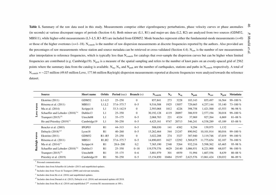
46P.M
ouliketal.
Table 1. Summary of the raw data used in this study. Measurements comprise either eigenfrequency perturbations, phase velocity curves or phase anomalies
(in seconds) at various discrepant ranges of periods (Section 4.4). Both minor-arc (L1, R1) and major-arc data (L2, R2) are analyzed from two sources (GDM52,
MBS11), while higher-orbit measurements (L3–L5, R3–R5) are included from GDM52. Mode branches represent either the fundamental-mode measurements (n=0)
or those of the higher overtones (n=1–18). Ncontrib is the number of raw dispersion measurements at discrete frequencies reported by the authors. Also provided are
the percentages of raw measurements whose station and source metadata can be retrieved or cross-validated (Section 4.4). Nraw is the number of raw measurements
after interpolation to reference frequencies, which is typically less than Ncontrib for catalogs that over-sample the dispersion curves but can be higher when limited
frequencies are contributed (e.g. Cambridge19). Ngrid is a measure of the spatial sampling and refers to the number of knot pairs on an evenly-spaced grid of 2562
points where the summary data from the catalog is available. Neq, Nst and Npath are the number of earthquakes, stations and paths in Ncontrib respectively. A total of
Ncontrib =∼227 million (49.65 million Love, 177.66 million Rayleigh) dispersion measurements reported at discrete frequencies were analyzed towards the reference
dataset.
Source Short name Orbits Period (sec) Branch (n) Ncontrib Nst Neq Npath Nraw Ngrid Metadata
Lov
ew
aves
Ekstrom (2011) GDM52 L1–L5 25–250 0 857,841 273 3228 103,143 855,497 16,564 99–100 %Ritsema et al. (2011) MBS11 L1,L2 37.6–375.7 0–5 9,516,508 1925 13057 729,665 4,257,144 55,140 73–100 %Ma et al. (2014) Scripps14 L1 33.3–142.9 0 2,593,068 1812 4226 398,758 1,421,500 43,553 96–98 %Schaeffer and Lebedev (2018)†a Dublin13 L1 25–350 0 30,192,128 4119 20097 306,919 2,577,194 30,018 99–100 %Trampert (2015)†b Utrecht08 L1 35–175 0–5 2,068,783 221 4324 37,969 927,264 6,869 81–88 %Ho and Priestley (2019)†c Cambridge19 L1 50–250 0–5 4,425,161 9747 20713 546,241 4,538,289 45,189 83–88 %
Ray
leig
hw
aves
Beucler et al. (2003) IPGP03 R1 44–315 0–5 508,030 141 4382 9,294 139,975 1,132 —Debayle (2018)†d Lyon18 R1 40–260 0–5 15,262,464 544 21247 890,942 10,101,914 80,016 99–100 %Ekstrom (2011) GDM52 R1–R5 25–250 0 3,022,208 274 3327 307,940 3,119,746 47,019 99–100 %Ritsema et al. (2011) MBS11 R1,R2 37.6–375.7 0–5 14,890,693 1627 12292 1,569,675 11,775,654 82,107 70–100 %Ma et al. (2014)†e Scripps14 R1 28.6–200 0,2 7,365,190 2348 5264 932,216 5,598,362 65,465 95–98 %Schaeffer and Lebedev (2018)†a Dublin13 R1 25–350 0–18 119,579,376 4629 24140 1,006,931 8,221,900 68,037 96–100 %Trampert (2015)†b Utrecht08 R1 35–175 0–6 3,881,979 301 6939 51,994 1,607,556 8,639 80–88 %Priestley et al. (2019) Cambridge19 R1 50–250 0–5 13,154,850 10484 25197 2,623,576 13,861,424 120,032 86–89 %
† Personal communication.a Includes data from Schaeffer & Lebedev (2013) and unpublished updates.b Includes data from Visser & Trampert (2008) and relevant metadata.c Includes data from Ho et al. (2016) and unpublished updates.d Includes data from Durand et al. (2015), Debayle et al. (2016) and automated updates till 2018.e Includes data from Ma et al. (2014) and unpublished 2nd overtone R1 measurements at 100 s.
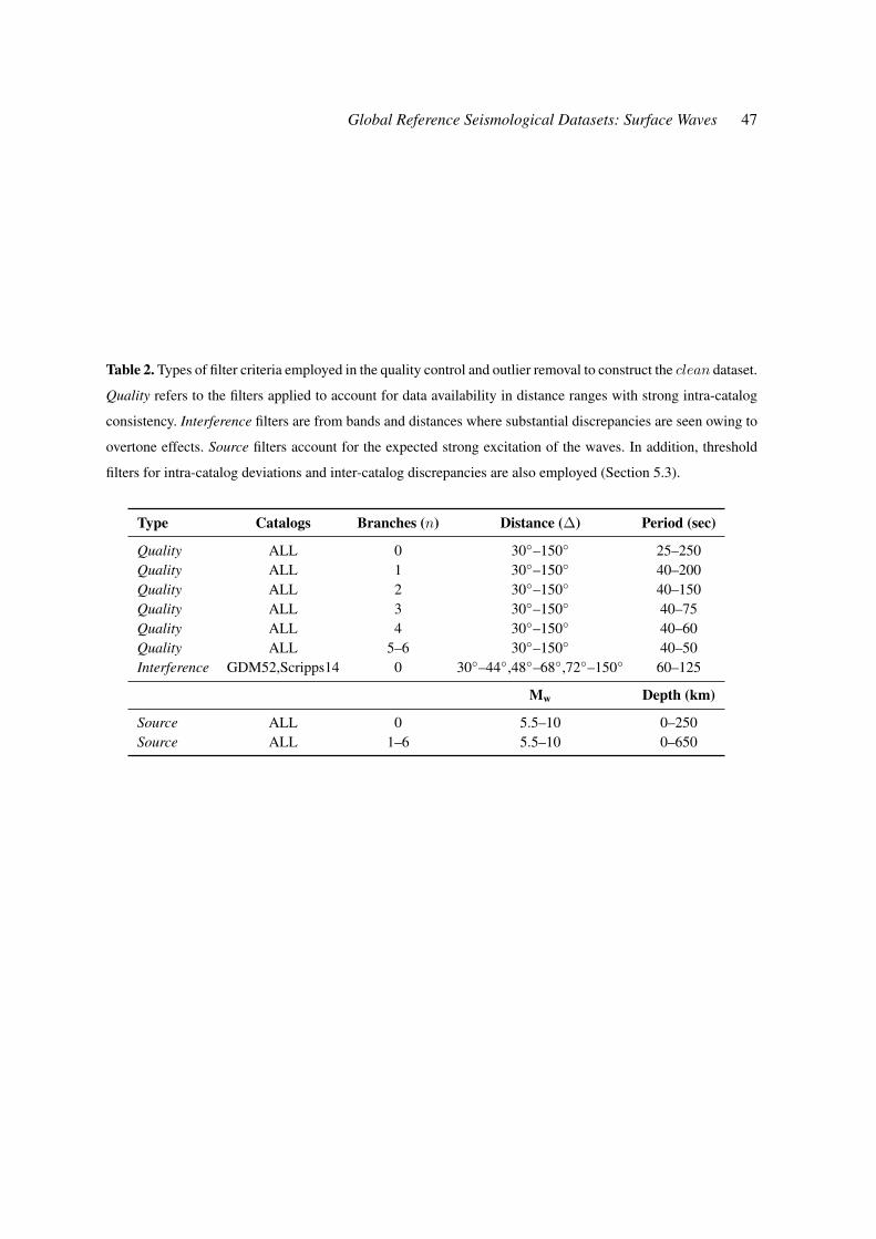
Global Reference Seismological Datasets: Surface Waves 47
Table 2. Types of filter criteria employed in the quality control and outlier removal to construct the clean dataset.
Quality refers to the filters applied to account for data availability in distance ranges with strong intra-catalog
consistency. Interference filters are from bands and distances where substantial discrepancies are seen owing to
overtone effects. Source filters account for the expected strong excitation of the waves. In addition, threshold
filters for intra-catalog deviations and inter-catalog discrepancies are also employed (Section 5.3).
Type Catalogs Branches (n) Distance (∆) Period (sec)
Quality ALL 0 30–150 25–250Quality ALL 1 30–150 40–200Quality ALL 2 30–150 40–150Quality ALL 3 30–150 40–75Quality ALL 4 30–150 40–60Quality ALL 5–6 30–150 40–50Interference GDM52,Scripps14 0 30–44,48–68,72–150 60–125
Mw Depth (km)
Source ALL 0 5.5–10 0–250Source ALL 1–6 5.5–10 0–650
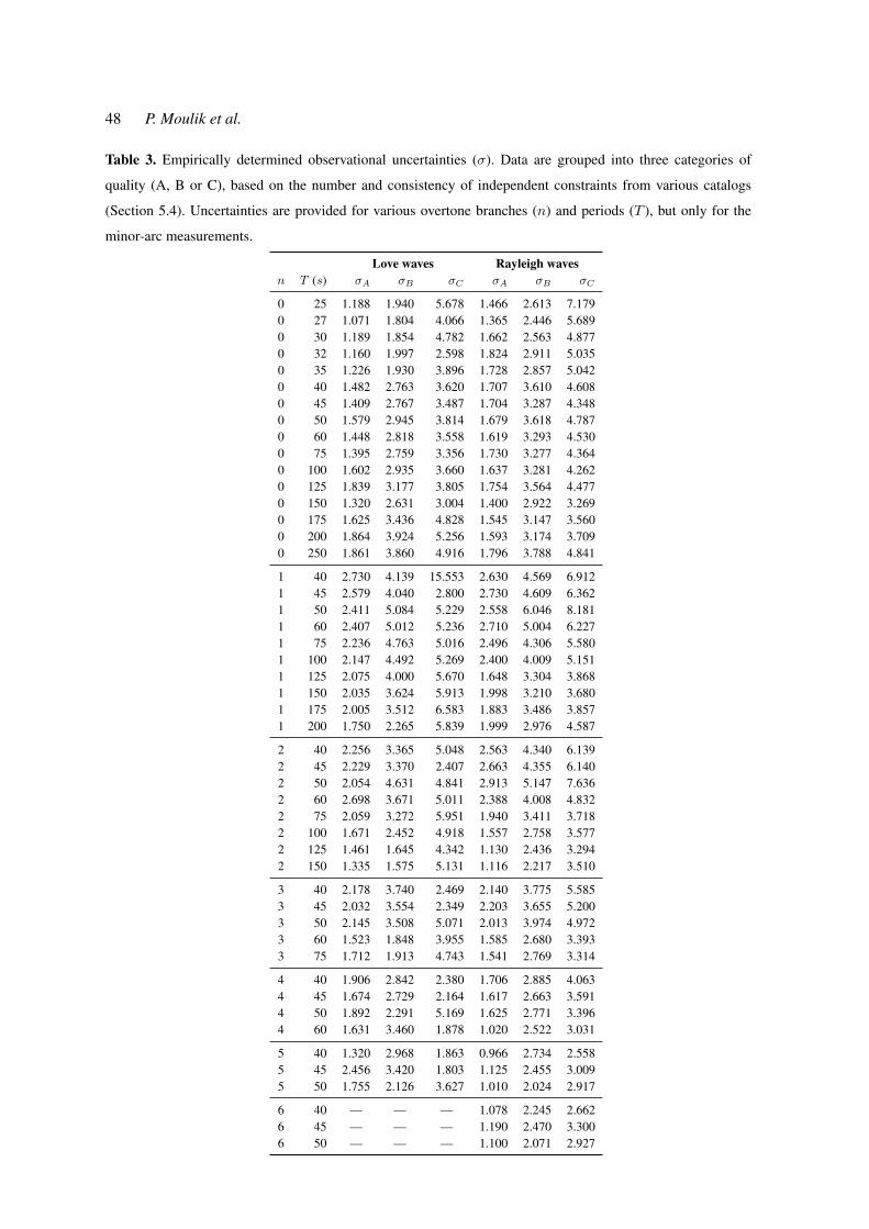
48 P. Moulik et al.
Table 3. Empirically determined observational uncertainties (σ). Data are grouped into three categories of
quality (A, B or C), based on the number and consistency of independent constraints from various catalogs
(Section 5.4). Uncertainties are provided for various overtone branches (n) and periods (T ), but only for the
minor-arc measurements.
Love waves Rayleigh wavesn T (s) σA σB σC σA σB σC
0 25 1.188 1.940 5.678 1.466 2.613 7.1790 27 1.071 1.804 4.066 1.365 2.446 5.6890 30 1.189 1.854 4.782 1.662 2.563 4.8770 32 1.160 1.997 2.598 1.824 2.911 5.0350 35 1.226 1.930 3.896 1.728 2.857 5.0420 40 1.482 2.763 3.620 1.707 3.610 4.6080 45 1.409 2.767 3.487 1.704 3.287 4.3480 50 1.579 2.945 3.814 1.679 3.618 4.7870 60 1.448 2.818 3.558 1.619 3.293 4.5300 75 1.395 2.759 3.356 1.730 3.277 4.3640 100 1.602 2.935 3.660 1.637 3.281 4.2620 125 1.839 3.177 3.805 1.754 3.564 4.4770 150 1.320 2.631 3.004 1.400 2.922 3.2690 175 1.625 3.436 4.828 1.545 3.147 3.5600 200 1.864 3.924 5.256 1.593 3.174 3.7090 250 1.861 3.860 4.916 1.796 3.788 4.841
1 40 2.730 4.139 15.553 2.630 4.569 6.9121 45 2.579 4.040 2.800 2.730 4.609 6.3621 50 2.411 5.084 5.229 2.558 6.046 8.1811 60 2.407 5.012 5.236 2.710 5.004 6.2271 75 2.236 4.763 5.016 2.496 4.306 5.5801 100 2.147 4.492 5.269 2.400 4.009 5.1511 125 2.075 4.000 5.670 1.648 3.304 3.8681 150 2.035 3.624 5.913 1.998 3.210 3.6801 175 2.005 3.512 6.583 1.883 3.486 3.8571 200 1.750 2.265 5.839 1.999 2.976 4.587
2 40 2.256 3.365 5.048 2.563 4.340 6.1392 45 2.229 3.370 2.407 2.663 4.355 6.1402 50 2.054 4.631 4.841 2.913 5.147 7.6362 60 2.698 3.671 5.011 2.388 4.008 4.8322 75 2.059 3.272 5.951 1.940 3.411 3.7182 100 1.671 2.452 4.918 1.557 2.758 3.5772 125 1.461 1.645 4.342 1.130 2.436 3.2942 150 1.335 1.575 5.131 1.116 2.217 3.510
3 40 2.178 3.740 2.469 2.140 3.775 5.5853 45 2.032 3.554 2.349 2.203 3.655 5.2003 50 2.145 3.508 5.071 2.013 3.974 4.9723 60 1.523 1.848 3.955 1.585 2.680 3.3933 75 1.712 1.913 4.743 1.541 2.769 3.314
4 40 1.906 2.842 2.380 1.706 2.885 4.0634 45 1.674 2.729 2.164 1.617 2.663 3.5914 50 1.892 2.291 5.169 1.625 2.771 3.3964 60 1.631 3.460 1.878 1.020 2.522 3.031
5 40 1.320 2.968 1.863 0.966 2.734 2.5585 45 2.456 3.420 1.803 1.125 2.455 3.0095 50 1.755 2.126 3.627 1.010 2.024 2.917
6 40 — — — 1.078 2.245 2.6626 45 — — — 1.190 2.470 3.3006 50 — — — 1.100 2.071 2.927
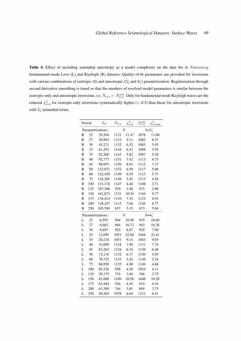
Global Reference Seismological Datasets: Surface Waves 49
Table 4. Effect of including azimuthal anisotropy as a model complexity on the data fits to Summary
fundamental-mode Love (L) and Rayleigh (R) datasets. Quality-of-fit parameters are provided for inversions
with various combinations of isotropic (0) and anisotropic (2ζ and 4ζ) parametrization. Regularization through
second derivative smoothing is tuned so that the numbers of resolved model parameters is similar between the
isotropic-only and anisotropic inversions, i.e.Nres ∼ Nanires . Only for fundamental mode Rayleigh waves are the
reduced χ2red for isotropic-only inversions systematically higher (> 0.3) than those for anisotropic inversions
with 2ζ azimuthal terms.
Period Nd Nres χ2red Nani
res χ2red,ani
Parametrizations : 0 0+2ζR 25 29,504 1131 11.47 1078 11.00R 27 29,893 1133 9.11 1082 8.57R 30 43,271 1132 6.52 1083 5.93R 32 61,293 1144 6.47 1098 5.95R 35 62,266 1143 5.82 1097 5.26R 40 92,777 1151 7.42 1113 6.73R 45 98,955 1150 8.01 1112 7.27R 50 122,071 1152 6.59 1117 5.88R 60 122,450 1149 6.54 1113 5.71R 75 124,205 1149 5.45 1113 4.56R 100 121,174 1147 4.48 1108 3.71R 125 107,368 970 3.48 975 2.96R 150 161,873 1121 10.54 1144 9.77R 175 138,414 1110 7.32 1122 6.91R 200 138,247 1112 7.04 1126 6.77R 250 105,599 837 5.15 873 5.04
Parametrizations : 0 0+4ζL 25 6,595 944 16.96 919 16.60L 27 6,662 964 16.72 943 16.28L 30 6,697 952 8.07 929 7.90L 32 12,095 1053 22.68 1044 22.41L 35 20,210 1051 9.14 1043 9.03L 40 53,699 1118 7.96 1131 7.74L 45 63,263 1124 6.74 1139 6.49L 50 72,116 1132 6.17 1150 5.95L 60 70,752 1133 5.45 1149 5.24L 75 68,958 1135 4.88 1149 4.68L 100 65,126 958 4.26 1010 4.11L 125 59,175 774 3.84 766 3.75L 150 81,088 1109 10.56 1048 10.28L 175 63,440 926 4.45 914 4.34L 200 63,389 744 3.81 694 3.75L 250 49,304 1078 6.64 1121 6.51
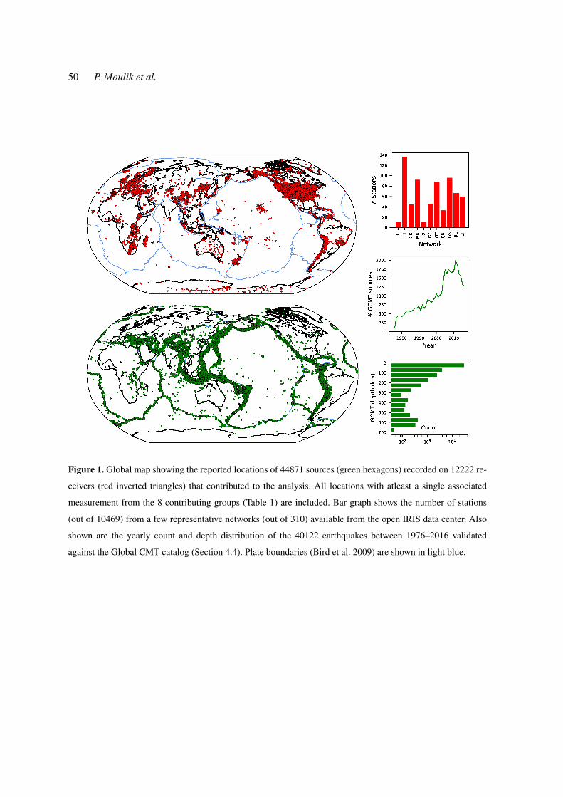
50 P. Moulik et al.
Figure 1. Global map showing the reported locations of 44871 sources (green hexagons) recorded on 12222 re-
ceivers (red inverted triangles) that contributed to the analysis. All locations with atleast a single associated
measurement from the 8 contributing groups (Table 1) are included. Bar graph shows the number of stations
(out of 10469) from a few representative networks (out of 310) available from the open IRIS data center. Also
shown are the yearly count and depth distribution of the 40122 earthquakes between 1976–2016 validated
against the Global CMT catalog (Section 4.4). Plate boundaries (Bird et al. 2009) are shown in light blue.
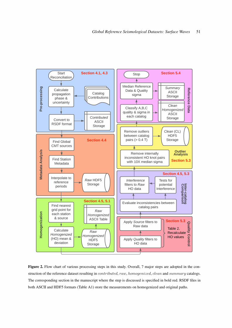
Global Reference Seismological Datasets: Surface Waves 51
Start Reconciliation
Convert to RSDF format
Pre
-pro
cess
ing
Find Global CMT sources
Find Station Metadata
Met
adat
a A
nal
ysis
Raw Homogenized
HDF5 Storage
Calculate Homogenized (HO) mean &
deviation
Interpolate to reference periods
Raw HDF5 Storage
Contributed ASCII
Storage
Ho
mo
gen
izat
ion
Find nearest grid point for each station
& source
Raw Homogenized ASCII Table
Qu
ality Co
ntro
l
Apply Quality filters to HO data
Table 2. Recalculate HO values
Apply Source filters to Raw data
Inter-catalo
g
Co
mp
arisonEvaluate inconsistencies between
catalog pairs
Interference filters to Raw
HO data
Tests for potential
Interference
Outlier AnalysisRemove internally
inconsistent HO knot pairs with 10X median sigma
Catalog Contributions
Stop
Clean (CL) HDF5
Storage
Remove outliers between catalog pairs (> 0.4 T)
Referen
ce Data
Classify A,B,C quality & sigma in
each catalog
Clean Homogenized
ASCII Storage
Median Reference Data & Quality
sigma
Summary ASCII
Storage
Calculate propagation
phase & uncertainty
Section 4.1, 4.3
Section 4.4
Section 4.5, 5.1
Section 5.3
Section 4.5, 5.3
Section 5.3
Section 5.4
Figure 2. Flow chart of various processing steps in this study. Overall, 7 major steps are adopted in the con-
struction of the reference dataset resulting in contributed, raw, homogenized, clean and summary catalogs.
The corresponding section in the manuscript where the step is discussed is specified in bold red. RSDF files in
both ASCII and HDF5 formats (Table A1) store the measurements on homogenized and original paths.
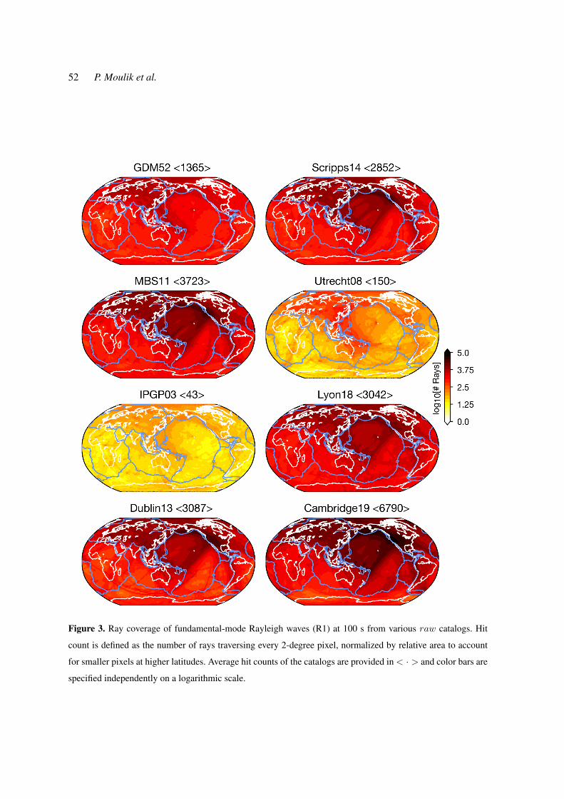
52 P. Moulik et al.
Figure 3. Ray coverage of fundamental-mode Rayleigh waves (R1) at 100 s from various raw catalogs. Hit
count is defined as the number of rays traversing every 2-degree pixel, normalized by relative area to account
for smaller pixels at higher latitudes. Average hit counts of the catalogs are provided in < · > and color bars are
specified independently on a logarithmic scale.
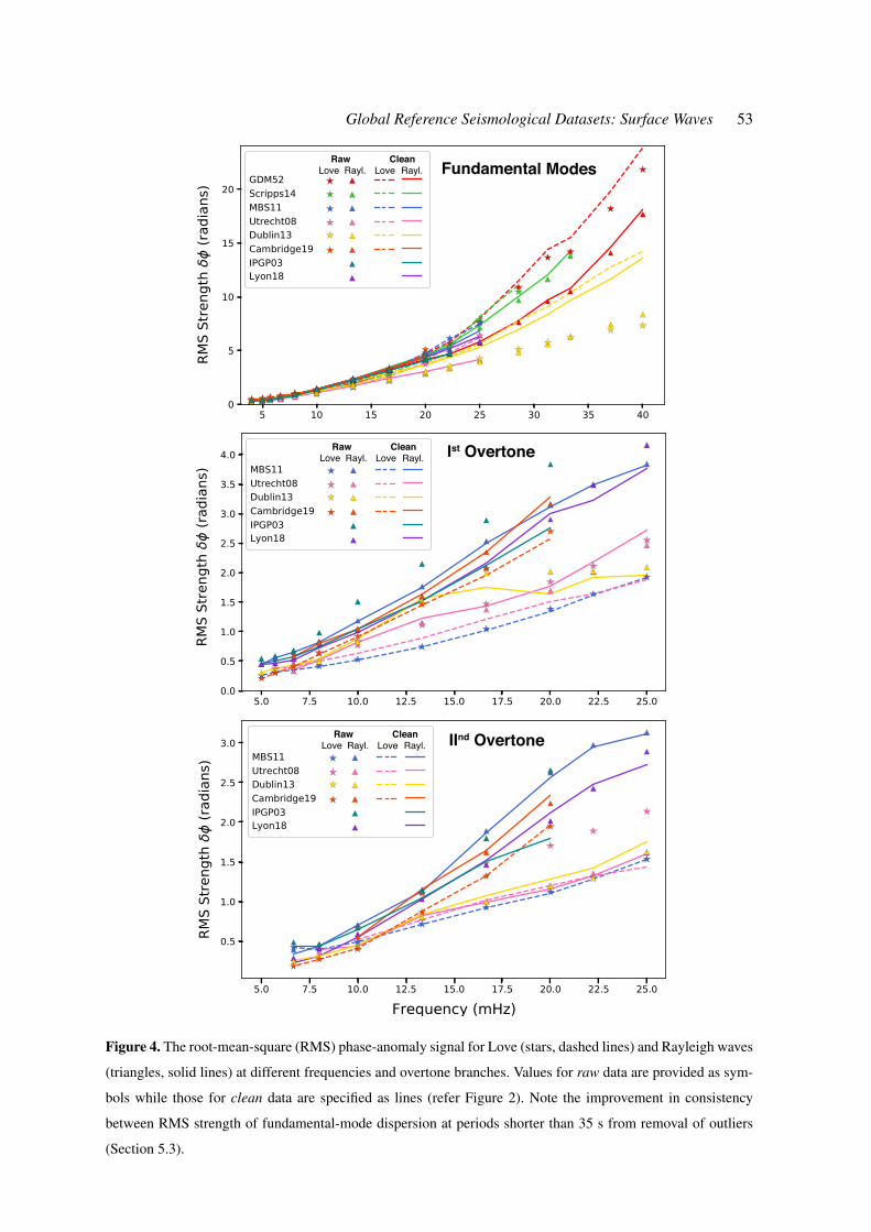
Global Reference Seismological Datasets: Surface Waves 53
Fundamental Modes
Ist Overtone
IInd Overtone
Love Rayl. Love Rayl.Raw Clean
Love Rayl. Love Rayl.Raw Clean
Love Rayl. Love Rayl.Raw Clean
Figure 4. The root-mean-square (RMS) phase-anomaly signal for Love (stars, dashed lines) and Rayleigh waves
(triangles, solid lines) at different frequencies and overtone branches. Values for raw data are provided as sym-
bols while those for clean data are specified as lines (refer Figure 2). Note the improvement in consistency
between RMS strength of fundamental-mode dispersion at periods shorter than 35 s from removal of outliers
(Section 5.3).

54 P. Moulik et al.
Figure 5. Scatter density plot of 66787 raw propagation phase anomaly measurements for 100 s R1 waves
common to both GDM52 (δφ1) and Lyon18 catalogs (δφ2). Scatter points are colored based on the spatial
density of nearby points, with high density in red and low density in blue. Histogram of the differences between
the reported measurements (δφ2-δφ1) on a logarithmic scale. Note the full-cycle (2π) band of discrepancies
between the catalogs for a small subset of common paths (∼1000) that also manifest as minor peaks in the
histogram. GDM52 reports slower velocities with arrival times that are 1.4 s longer on average than Lyon18.
Both mean and median of the absolute differences in measurements binned every 2 show a linear increase
with great-circle distance between the source and receiver. Such minor discrepancies may arise from discrepant
theoretical approximations, reference Earth models and processing schemes.
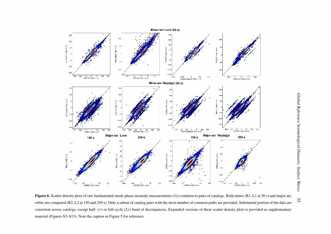
GlobalR
eferenceSeism
ologicalDatasets:Surface
Waves
55
Figure 6. Scatter density plots of raw fundamental-mode phase-anomaly measurements (δφ) common to pairs of catalogs. Both minor (R1, L1 at 50 s) and major-arc
orbits are compared (R2, L2 at 150 and 250 s). Only a subset of catalog pairs with the most number of common paths are provided. Substantial portion of the data are
consistent across catalogs, except half- (π) or full-cycle (2π) band of discrepancies. Expanded versions of these scatter density plots is provided as supplementary
material (Figures S2–S13). Note the caption in Figure 5 for reference.
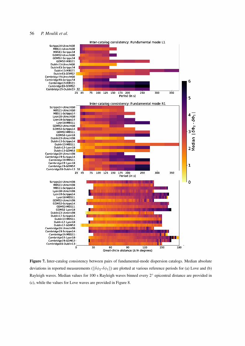
56 P. Moulik et al.
Figure 7. Inter-catalog consistency between pairs of fundamental-mode dispersion catalogs. Median absolute
deviations in reported measurements (‖δφ2-δφ1‖) are plotted at various reference periods for (a) Love and (b)
Rayleigh waves. Median values for 100 s Rayleigh waves binned every 2 epicentral distance are provided in
(c), while the values for Love waves are provided in Figure 8.

Global Reference Seismological Datasets: Surface Waves 57
Figure 8. Influence of overtone interference on dispersion measurements of fundamental modes. (a) Obser-
vations of discrepancies between fundamental-mode and multi-mode techniques at specific source-station dis-
tances, highlighted with circles in grey. Note the caption in Figure 7 for reference. Amplitude ratios (b-c) and
instantaneous phase (d) between the envelopes of synthetics from various combinations of overtone branches
and radial (1D) models. Synthetics are created from an average global model (STW105, Kustowski et al. 2008),
and from oceanic and continental profiles constructed using the GTR1 tectonic regionalization (Jordan 1981).
All synthetic waveforms are narrow-pass filtered between 8-12 mHz.

58P.M
ouliketal.
Figure 9. Scatter density plots of raw overtone phase-anomaly measurements (δΦ) common to pairs of catalogs. Overtone measurements for branches 1–6 are
compared for minor-arc orbits (R1, L1) at 50 s and only the subset of combinations with the most number of common paths are shown. Expanded versions of these
scatter density plots is provided as supplementary material (Figures S14–S25). Note the caption in Figure 5 for reference.
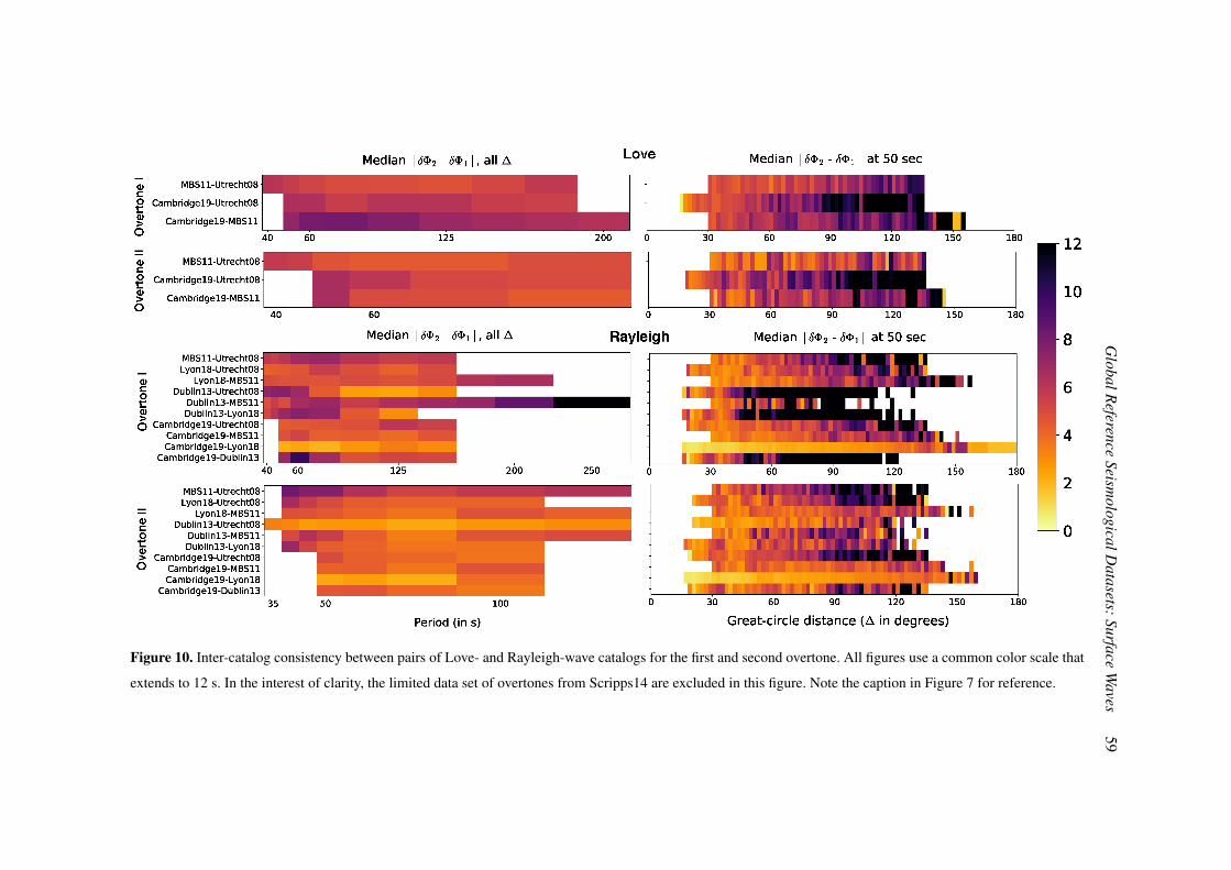
GlobalR
eferenceSeism
ologicalDatasets:Surface
Waves
59
Figure 10. Inter-catalog consistency between pairs of Love- and Rayleigh-wave catalogs for the first and second overtone. All figures use a common color scale that
extends to 12 s. In the interest of clarity, the limited data set of overtones from Scripps14 are excluded in this figure. Note the caption in Figure 7 for reference.
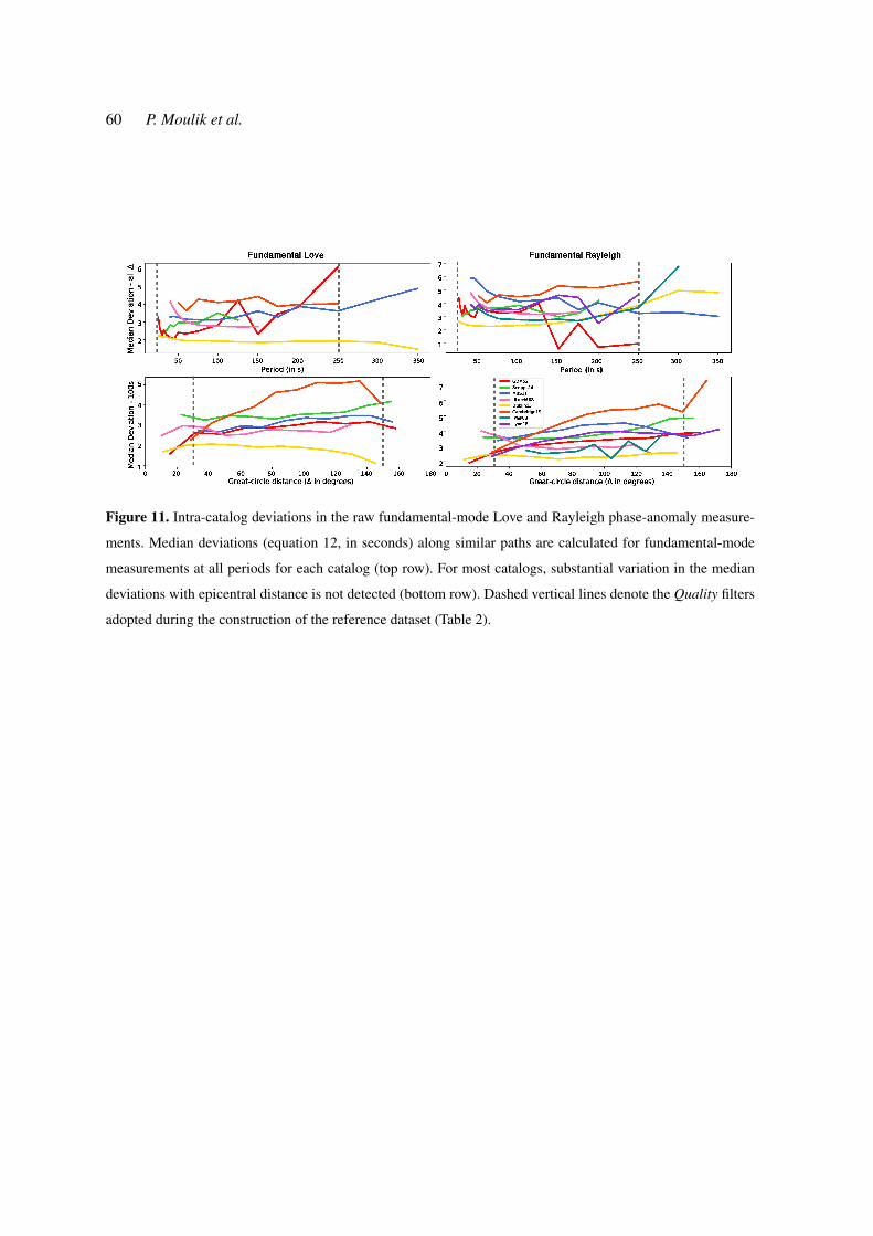
60 P. Moulik et al.
Figure 11. Intra-catalog deviations in the raw fundamental-mode Love and Rayleigh phase-anomaly measure-
ments. Median deviations (equation 12, in seconds) along similar paths are calculated for fundamental-mode
measurements at all periods for each catalog (top row). For most catalogs, substantial variation in the median
deviations with epicentral distance is not detected (bottom row). Dashed vertical lines denote the Quality filters
adopted during the construction of the reference dataset (Table 2).
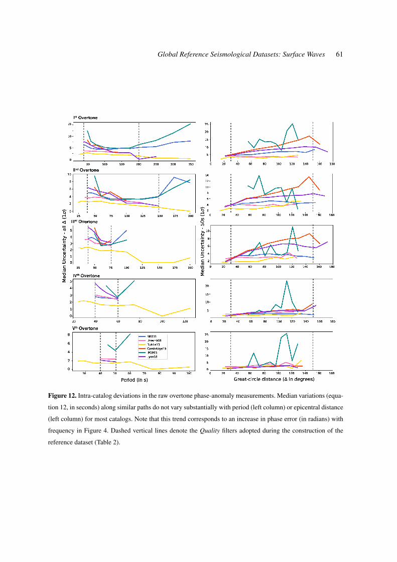
Global Reference Seismological Datasets: Surface Waves 61
Figure 12. Intra-catalog deviations in the raw overtone phase-anomaly measurements. Median variations (equa-
tion 12, in seconds) along similar paths do not vary substantially with period (left column) or epicentral distance
(left column) for most catalogs. Note that this trend corresponds to an increase in phase error (in radians) with
frequency in Figure 4. Dashed vertical lines denote the Quality filters adopted during the construction of the
reference dataset (Table 2).
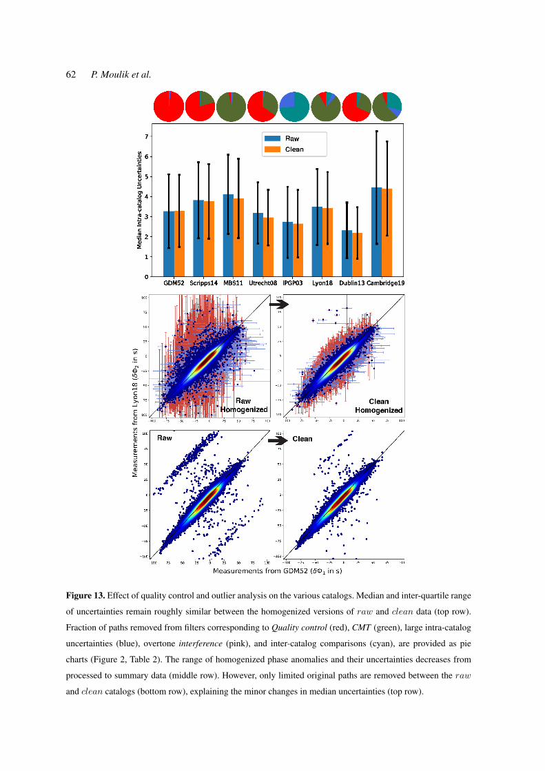
62 P. Moulik et al.
Figure 13. Effect of quality control and outlier analysis on the various catalogs. Median and inter-quartile range
of uncertainties remain roughly similar between the homogenized versions of raw and clean data (top row).
Fraction of paths removed from filters corresponding to Quality control (red), CMT (green), large intra-catalog
uncertainties (blue), overtone interference (pink), and inter-catalog comparisons (cyan), are provided as pie
charts (Figure 2, Table 2). The range of homogenized phase anomalies and their uncertainties decreases from
processed to summary data (middle row). However, only limited original paths are removed between the raw
and clean catalogs (bottom row), explaining the minor changes in median uncertainties (top row).

Global Reference Seismological Datasets: Surface Waves 63
Figure 14. Half-cycle (π) discrepancies between pairs of catalogs, attributed to polarity reversals in waveform
data. These issues are preferentially observed at epicentral distances∼77–92 and on certain dates and stations.
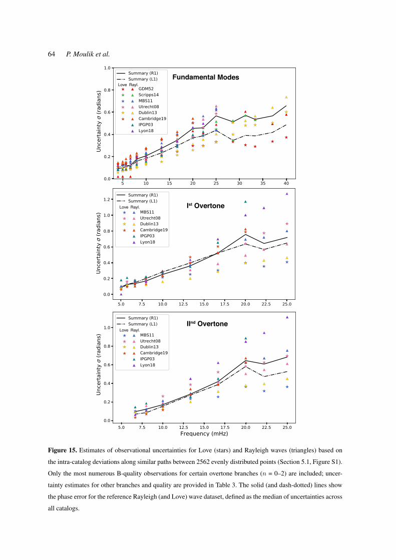
64 P. Moulik et al.
Fundamental Modes
Ist Overtone
IInd Overtone
Love Rayl.
Love Rayl.
Love Rayl.
Figure 15. Estimates of observational uncertainties for Love (stars) and Rayleigh waves (triangles) based on
the intra-catalog deviations along similar paths between 2562 evenly distributed points (Section 5.1, Figure S1).
Only the most numerous B-quality observations for certain overtone branches (n = 0–2) are included; uncer-
tainty estimates for other branches and quality are provided in Table 3. The solid (and dash-dotted) lines show
the phase error for the reference Rayleigh (and Love) wave dataset, defined as the median of uncertainties across
all catalogs.

Global Reference Seismological Datasets: Surface Waves 65
5 10 15 20 25 30Spherical Harmonic Degree
-3
-2.5
-2
-1.5
-1
-0.5
0
log 10
Pow
er
Spherical Harmonic Degree
-4
-3.5
-3
-2.5
-2
-1.5
-1
log
10 P
ower
5 10 15 20
Isotropic Terms Anisotropic Terms
λ = 1λ = 2λ = 3λ = 5λ = 8
λ = 13λ = 22λ = 36λ = 60λ = 100
Figure 16. Effect of smoothing applied to anisotropic terms (λ) on power spectra of isotropic and anisotropic
variations inverted from summary 100 s fundamental-mode Rayleigh wave measurements. Small values of λ re-
sult in overly smooth isotropic variations, and stronger anisotropic variations at shorter wavelengths (degrees 6).
The value λ = 8 is chosen as it yields a flat spectrum of anisotropic variations and does not substantially affect
isotropic variations below degree ∼ 24.
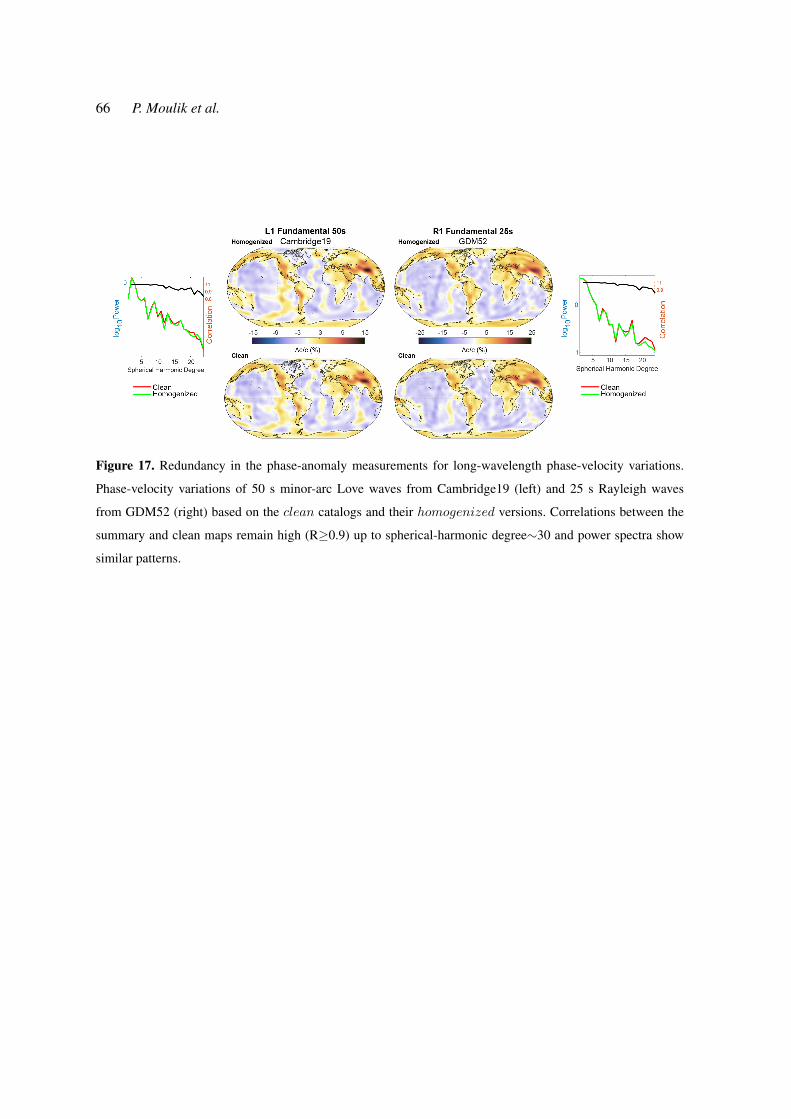
66 P. Moulik et al.
Figure 17. Redundancy in the phase-anomaly measurements for long-wavelength phase-velocity variations.
Phase-velocity variations of 50 s minor-arc Love waves from Cambridge19 (left) and 25 s Rayleigh waves
from GDM52 (right) based on the clean catalogs and their homogenized versions. Correlations between the
summary and clean maps remain high (R≥0.9) up to spherical-harmonic degree∼30 and power spectra show
similar patterns.
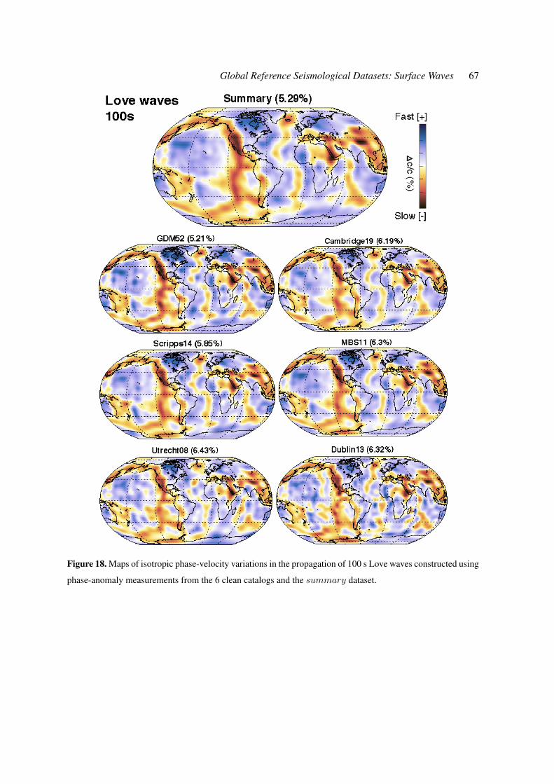
Global Reference Seismological Datasets: Surface Waves 67
Figure 18. Maps of isotropic phase-velocity variations in the propagation of 100 s Love waves constructed using
phase-anomaly measurements from the 6 clean catalogs and the summary dataset.
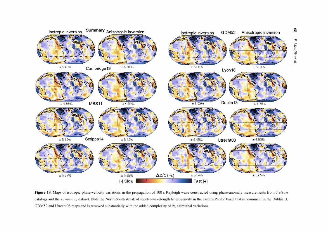
68P.M
ouliketal.
Figure 19. Maps of isotropic phase-velocity variations in the propagation of 100 s Rayleigh wave constructed using phase-anomaly measurements from 7 clean
catalogs and the summary dataset. Note the North-South streak of shorter-wavelength heterogeneity in the eastern Pacific basin that is prominent in the Dublin13,
GDM52 and Utrecht08 maps and is removed substantially with the added complexity of 2ζ azimuthal variations.
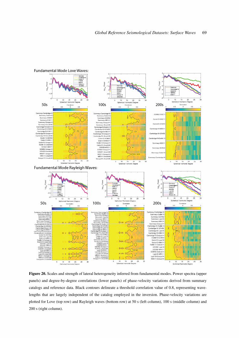
Global Reference Seismological Datasets: Surface Waves 69
Figure 20. Scales and strength of lateral heterogeneity inferred from fundamental modes. Power spectra (upper
panels) and degree-by-degree correlations (lower panels) of phase-velocity variations derived from summary
catalogs and reference data. Black contours delineate a threshold correlation value of 0.8, representing wave-
lengths that are largely independent of the catalog employed in the inversion. Phase-velocity variations are
plotted for Love (top row) and Rayleigh waves (bottom row) at 50 s (left column), 100 s (middle column) and
200 s (right column).
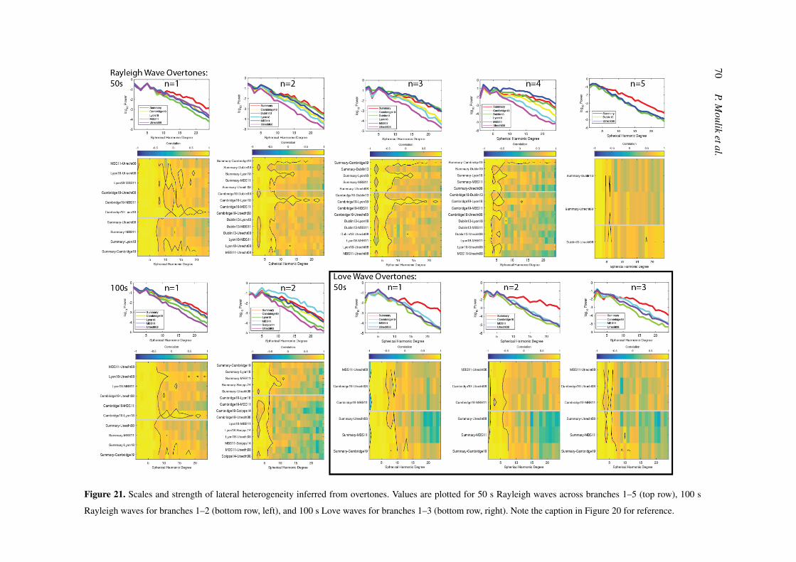
70P.M
ouliketal.
Figure 21. Scales and strength of lateral heterogeneity inferred from overtones. Values are plotted for 50 s Rayleigh waves across branches 1–5 (top row), 100 s
Rayleigh waves for branches 1–2 (bottom row, left), and 100 s Love waves for branches 1–3 (bottom row, right). Note the caption in Figure 20 for reference.

Global Reference Seismological Datasets: Surface Waves 71
Figure 22. Phase-velocity variations in 200 s Love and Rayleigh waves from minor arc (top row : L1,R1), major
arc (middle row : L2,R2), and higher orbit (bottom row : L3–L5,R3–R5) phase-anomaly measurements of the
reference dataset. Degree-by-degree correlations between maps are high up to degree 8, and persist up to degree
16 for even degrees (top) and power spectra show similar patterns (bottom).
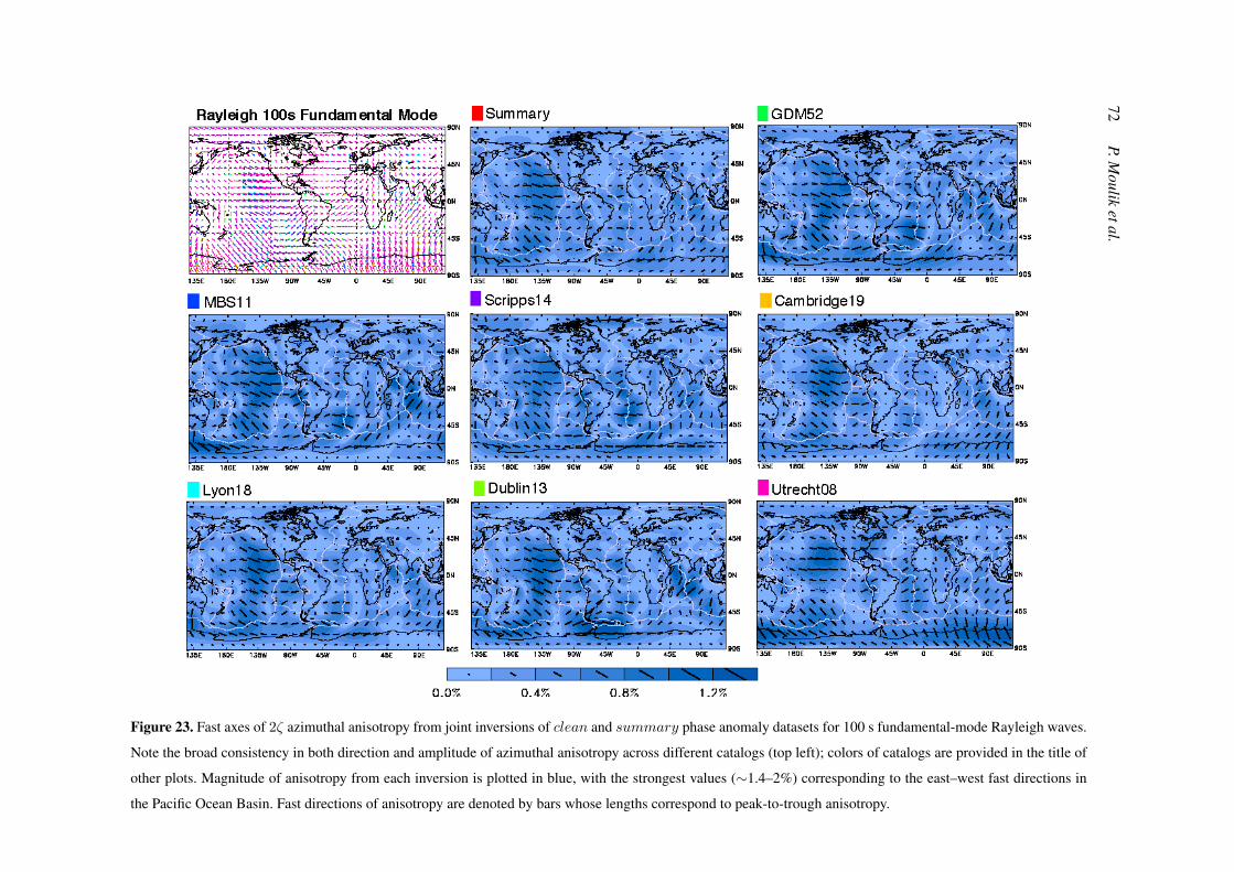
72P.M
ouliketal.
Figure 23. Fast axes of 2ζ azimuthal anisotropy from joint inversions of clean and summary phase anomaly datasets for 100 s fundamental-mode Rayleigh waves.
Note the broad consistency in both direction and amplitude of azimuthal anisotropy across different catalogs (top left); colors of catalogs are provided in the title of
other plots. Magnitude of anisotropy from each inversion is plotted in blue, with the strongest values (∼1.4–2%) corresponding to the east–west fast directions in
the Pacific Ocean Basin. Fast directions of anisotropy are denoted by bars whose lengths correspond to peak-to-trough anisotropy.

Global Reference Seismological Datasets: Surface Waves 73
APPENDIX A: SCALABLE STORAGE FORMATS1048
Measurements of surface-wave dispersion need to be cross-validated against source and station meta-1049
data to reference the appropriate seismic waveform and facilitate reproducible research. However, the1050
analysis of large amounts of data from diverse catalogs is computationally inefficient with conven-1051
tional ASCII and other text-based formats. We have devised reference seismic data formats (RSDFs)1052
in consultation with the community to efficiently process diverse datasets typically employed in seis-1053
mic tomography. While a general definition of a surface-wave format is desirable, practical consider-1054
ations such as diverse processing techniques, computational expertise and utilization of legacy code1055
prevent such an outcome throughout the community. RSDFs format guidelines (Table A1) encourage1056
easy tracking of critical metadata information as header information that will work within existing1057
processing schemes. Headers of RSDF ASCII files store all notes and details relevant to the analysis1058
such as the radial reference Earth model and the associated phase velocity (PVEL) used for calculat-1059
ing the reference phase (Φ0P , equation 7). Other metadata fields correspond to the assumptions used in1060
calculating the various columns in the data such as those contributing to the predicted phase anomaly1061
(δΦpred, Moulik & Ekstrom 2016, Appendix A). The format presented here includes the fields neces-1062
sary for data reconciliation; other (meta)data specific to a processing scheme can be preserved at the1063
discretion of the analyst.1064
The archival of millions of surface-wave measurements and associated metadata in the RSDF1065
definition requires an efficient container format. Each catalog is stored in a data container with the1066
metadata as attributes and folders for each wave type, overtone branch and frequency. We chose HDF51067
(Hierarchical Data Format version 5; The HDF Group 1997–2015) after extensive testing on various1068
computational platforms. First, HDF5 is widely used as a standard format for data exchange and is1069
operable on various operating systems and platforms. Programs in major languages (e.g. FORTRAN,1070
C and Python) can interface with HDF5 files and there is an active ecosystem with an abundance of1071
libraries and tools. Its usage is steadily increasing in seismology with the related NetCDF 4 definition1072
regularly used during the archival of Earth models and in the processing of waveforms (e.g. Krischer1073
et al. 2016). Second, HDF5 fulfills our requirement of efficient parallel I/O with MPI (message passing1074
interface; MPI Forum 2009) that is needed to process and compare various sets of catalogs. Third,1075
allied features such as the built-in data compression algorithms and data corruption tests in the form1076
of check summing facilitate efficient archival. In contrast to binary formats, HDF5 container formats1077
do not need to account for the endianness of the data and the associated compatibility issues across1078
computational environments.1079
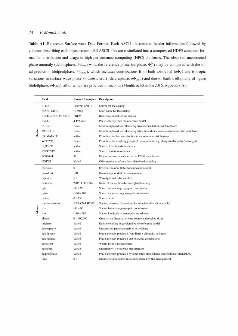
74 P. Moulik et al.
Table A1. Reference Surface-wave Data Format: Each ASCII file contains header information followed by
columns describing each measurement. All ASCII files are assimilated into a compressed HDF5 container for-
mat for distribution and usage in high performance computing (HPC) platforms. The observed uncorrected
phase anomaly (delobsphase, δΦobs) w.r.t. the reference phase (refphase, Φ0P ) may be compared with the to-
tal prediction (delpredphase, δΦpred), which includes contributions from both azimuthal (δΦζ) and isotropic
variations in surface-wave phase slowness, crust (delcruphase, δΦcrust) and due to Earth’s ellipticity of figure
(delellphase, δΦellip), all of which are provided in seconds (Moulik & Ekstrom 2016, Appendix A).
Field Range / Examples Description
Hea
der
CITE: Ekstrom (2011) Source for the catalog
SHORTCITE: GDM52 Short name for the catalog
REFERENCE MODEL: PREM Reference model for the catalog
PVEL: 4.492 km/s Phase velocity from the reference model
CRUST: None Model employed for calculating crustal contributions (delcruphase)
MODEL3D: None Model employed for calculating other three-dimensional contributions (delpredphase)
SIGMATYPE: author Procedure for 1-σ uncertainties in measurements (delsigma)
WEITYPE: None Procedure for weighing groups of measurements e.g. along similar paths (delweight)
EQTYPE: author Source of earthquake metadata
STATTYPE: author Source of station metadata
FORMAT: 99 Denotes measurements are in the RSDF data format
NOTES: Varied Other pertinent information related to the catalog
Col
umns
overtone 0 Overtone number (0 for fundamental modes)
period (s) 100 Dominant period of the measurement.
typeiorb R1 Wave type and orbit number
cmtname 200511142138A Name of the earthquake from globalcmt.org
eplat -90 – 90 Source latitude in geographic coordinates
eplon -180 – 180 Source longitude in geographic coordinates
cmtdep 0 – 750 Source depth
stat-net-chan-loc BBB-CN-LHT-00 Station, network, channel and location identifier (if available)
stlat -90 – 90 Station latitude in geographic coordinates
stlon -180 – 180 Station longitude in geographic coordinates
distkm 0 – 400,000 Great-circle distance between source and receiver (km)
refphase Varied Reference phase as predicted by the reference model
delobsphase Varied Uncorrected phase anomaly w.r.t. refphase
delellphase Varied Phase anomaly predicted from Earth’s ellipticity of figure
delcruphase Varied Phase anomaly predicted due to crustal contributions
delweight Varied Weight for this measurement
delsigma Varied Uncertainty (1-σ) for the measurement
delpredphase Varied Phase anomaly predicted by other three-dimensional contributions (MODEL3D)
iflag 0-9 Number of processing milestones cleared by the measurement
Related Documents