Multi Layer NN and Bit-True Modeling of These Networks SILab presentation Ali Ahmadi September 2007.

Multi Layer NN and Bit-True Modeling of These Networks

SILab presentation

Ali Ahmadi

September 2007

Outline

• Review structures of Single Layer Neural Networks

• Introduction to Multi Layer Perceptron (MLP) Neural Network

• Error Back-Propagation Learning Algorithm• MLP Model for XOR function and Digit

Recognition System

• Bit-True model of networks

Hopfield Network

-Single layer-Fully connected

[3]

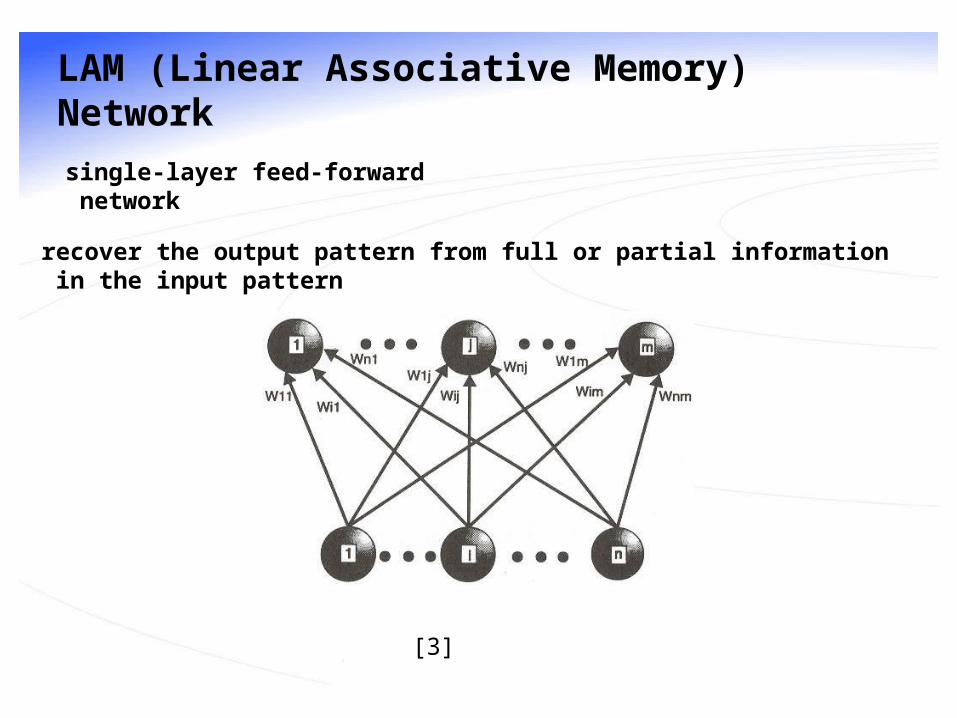
LAM (Linear Associative Memory) Network

single-layer feed-forward network

recover the output pattern from full or partial information in the input pattern

[3]

BAM (Bidirectional Associative Memory) Network

1 2 3 Y

1 2 X

bidirectional

Two layer with different dimension

For each pattern we have pair (a, b) related to each layer

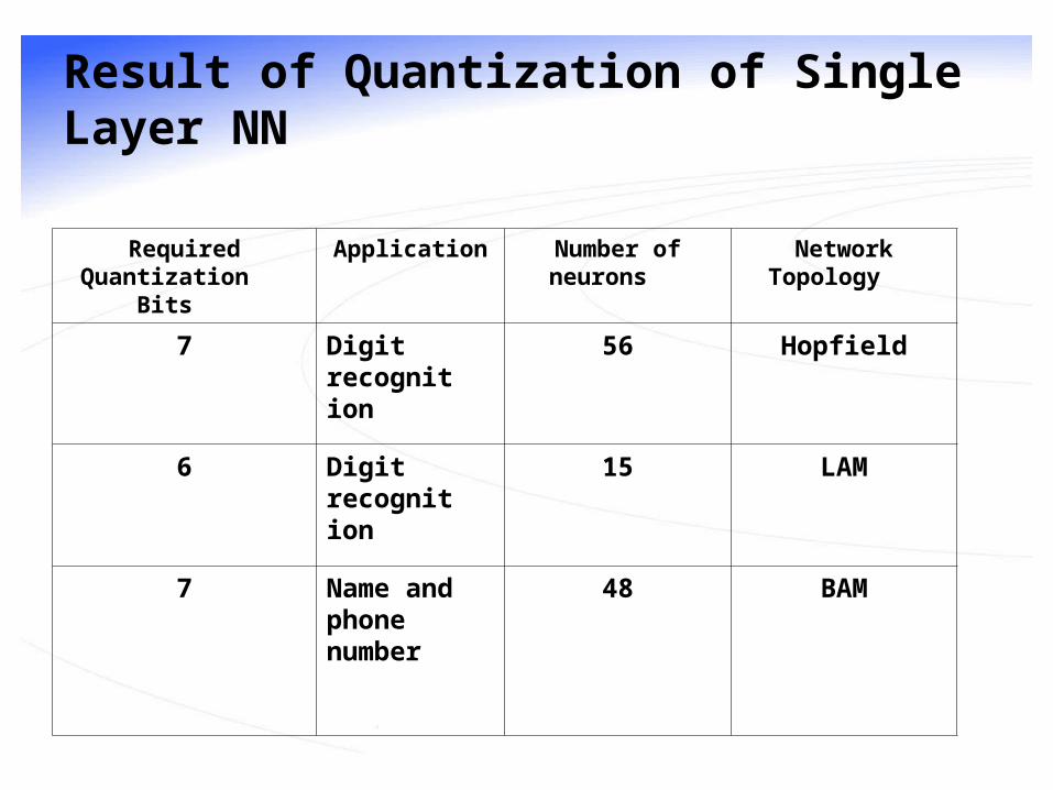
Result of Quantization of Single Layer NN

Network TopologyNumber of neuronsApplicationRequired Quantization Bits

Hopfield56Digit recognition

7

LAM15Digit recognition

6

BAM48Name and phone number

7

Why need Multi Layer Neural Networks?

• Classify objects by learning nonlinearity

• There are many problems for which linear discriminates are insufficient for minimum error

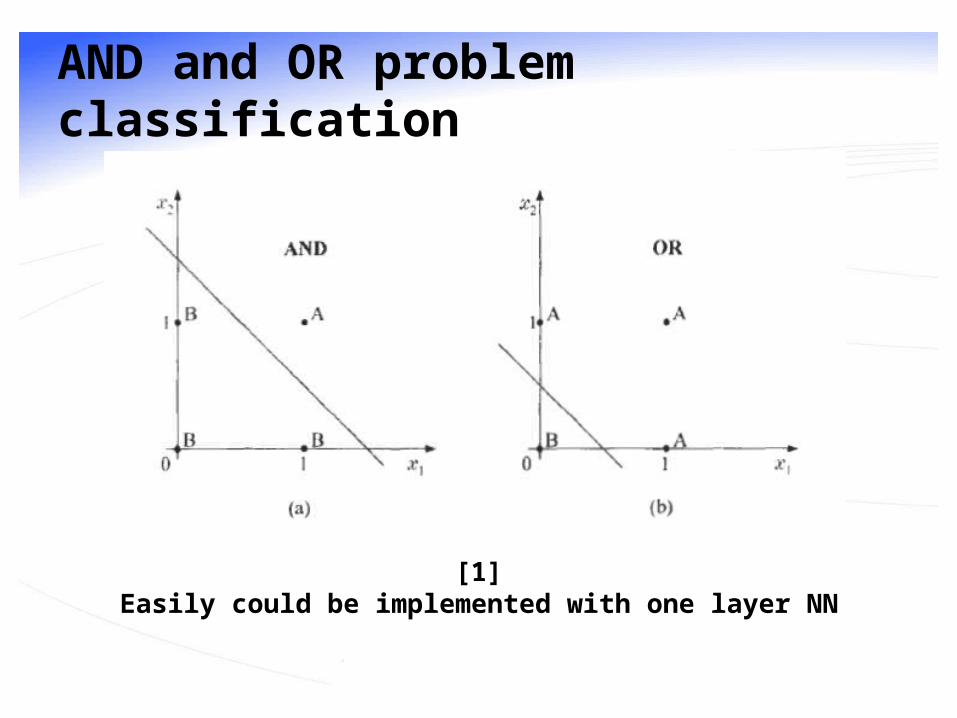
AND and OR problem classification

[1]Easily could be implemented with one layer NN

Classification of XOR problem

[1]It is nonlinear problem (couldn’t be implemented with single layer NN)

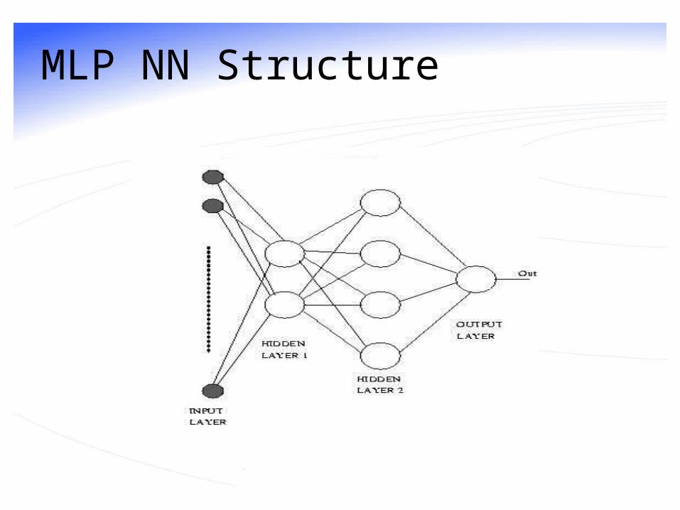
MLP NN Structure

Feed-forward Operation (input-to hidden)

d

1i

d

0i

tjjii0jjiij ,x.wwxwwxnet

In MLPs a single “bias unit” is connected to each unit other than the input units

Indexes i for input layer units, j in the hidden; wji denotes the input-to-hidden layer weights at the hidden unit j. wj0 is for bias unit of neuron j in hidden layer

Each hidden unit emits an output that is a nonlinear function of its activation, that is:

yj = f(netj)

Feed-forward Operation (hidden-to-output)

Each output unit net activation based on the hidden unit signals as:

subscript k indexes units in the output layer and nH denotes the number of hidden units

final output of each neuron in output layer

zk = f(netk)

H Hn

1j

n

0j

tkkjj0kkjjk ,y.wwywwynet

Expressive Power of multi-layer Networks

• Any continuous function from input to output can be implemented in a three-layer net, given sufficient number of hidden units nH, proper nonlinearities, and weights[2].

Error Back-Propagation Algorithm

• Back-propagation is one of the simplest and most general methods for training of multilayer neural networks.

• The power of back-propagation is that it enables us to compute an effective error for each hidden unit, and thus derive a learning rule for the input-to-hidden weights.

• Our goal now is to set the interconnection weights based on the training patterns and the desired outputs

• Slow convergence speed, is Disadvantages of error back-propagation algorithm.

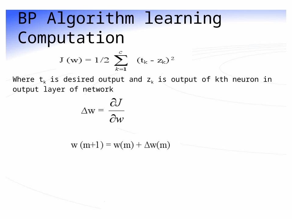
BP Algorithm learning Computation

Where tk is desired output and zk is output of kth neuron in output layer of network

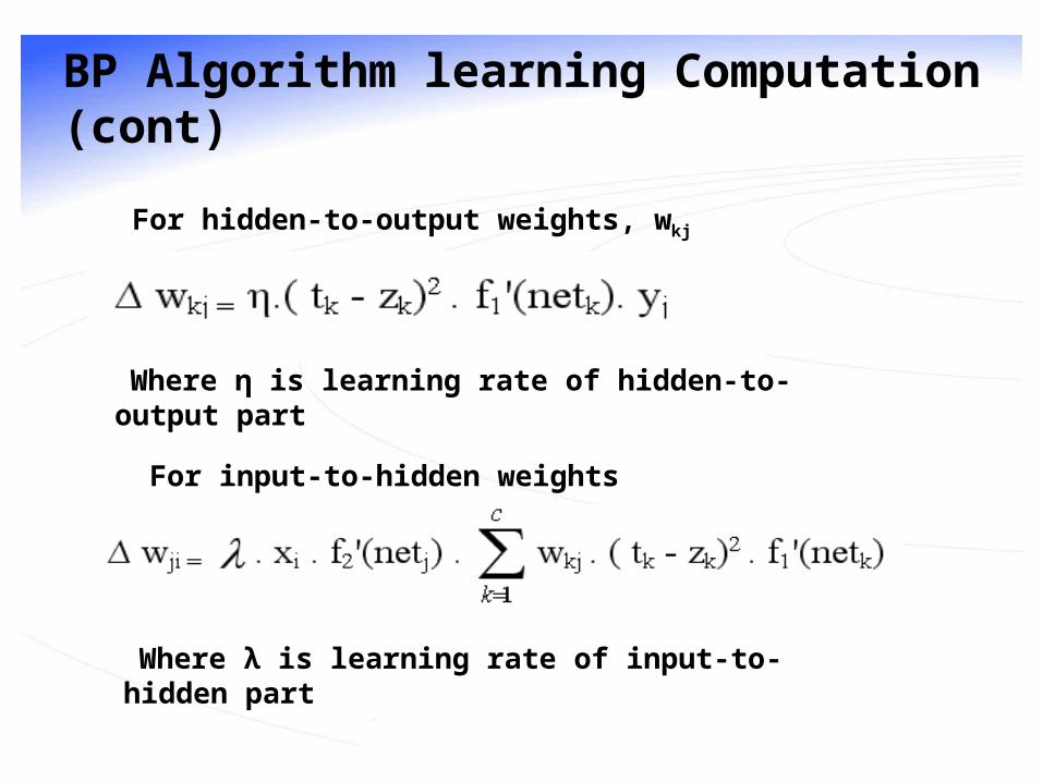
BP Algorithm learning Computation (cont)

For hidden-to-output weights, wkj

Where η is learning rate of hidden-to-output part

For input-to-hidden weights

Where λ is learning rate of input-to-hidden part

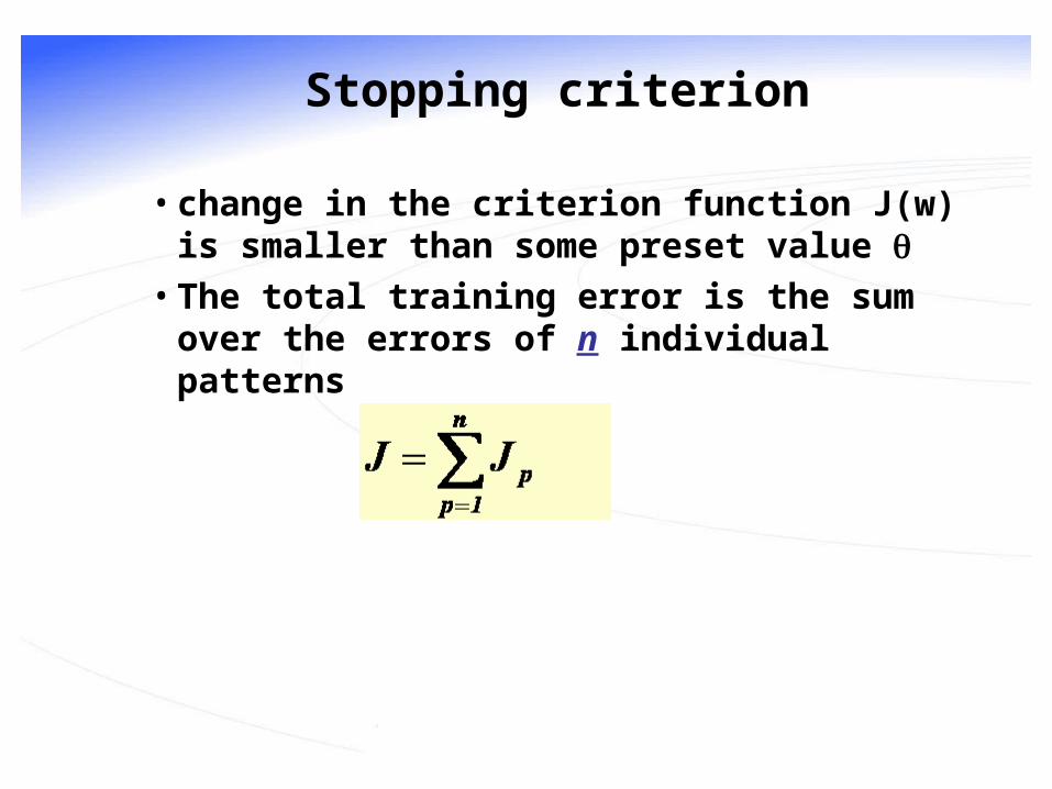
Stopping criterion

• change in the criterion function J(w) is smaller than some preset value

• The total training error is the sum over the errors of n individual patterns

BP Algorithm

• begin initialize network topology(# hidden units),w, criterion

θ, η,m ← 0

do m ← m + 1

xm ← randomly chosen pattern

wij ← wij + ηδjxi;

wjk ← wjk + ηδk yj

until ▼J(w) < θ return w• end

• Network have two modes of operation:

– Feed-forward

The feed-forward operations consists of presenting a pattern to the input units and passing (or feeding) the signals through the network in order to get outputs units

– Learning

The learning consists of presenting an input pattern and modifying the network parameters (weights) to reduce distances between the computed output and the desired output

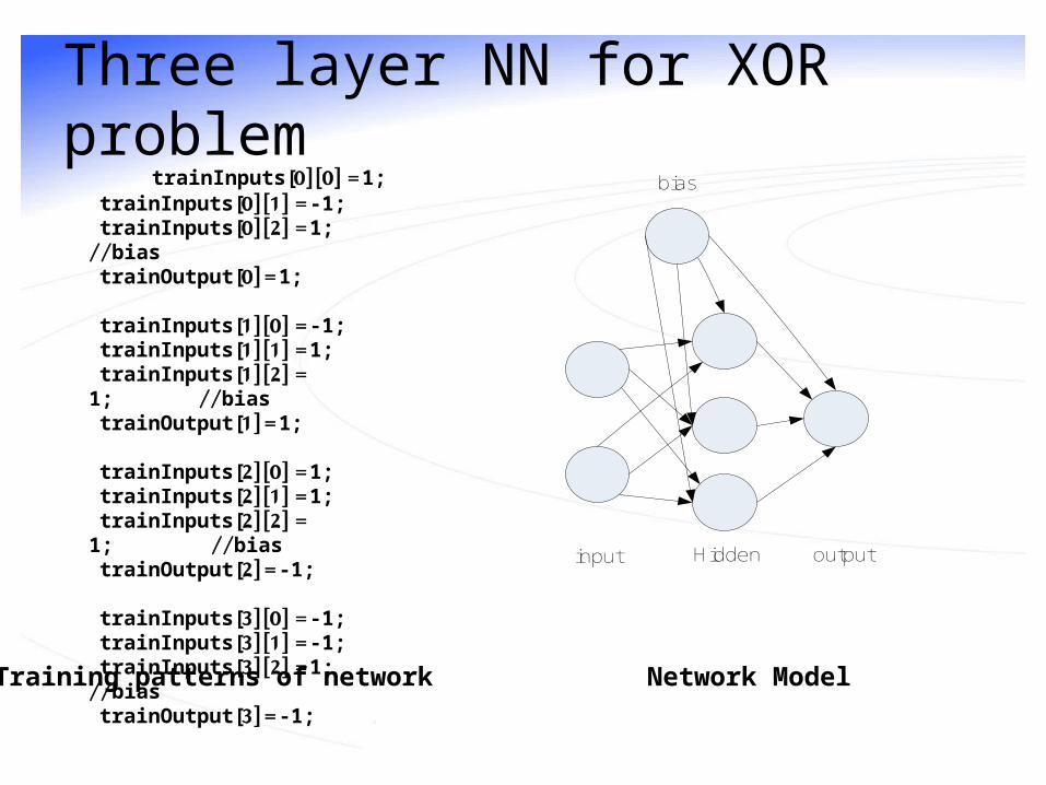
Three layer NN for XOR problem

input Hidden output

bias trainInputs[0][0] = 1; trainInputs[0][1] = -1; trainInputs[0][2] = 1; //bias trainOutput[0] = 1;

trainInputs[1][0] = -1; trainInputs[1][1] = 1; trainInputs[1][2] = 1; //bias trainOutput[1] = 1;

trainInputs[2][0] = 1; trainInputs[2][1] = 1; trainInputs[2][2] = 1; //bias trainOutput[2] = -1;

trainInputs[3][0] = -1; trainInputs[3][1] = -1; trainInputs[3][2] = 1; //bias trainOutput[3] = -1;

Network ModelTraining patterns of network

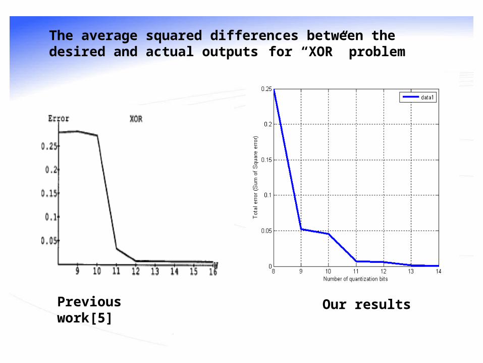
The average squared differences between the desired and actual outputs for “XOR” problem

Our resultsPrevious work[5]

Three layer MLP for pattern recognition

1

4

2

16

1

1

22

3

13

Input layer Hiddden layer Output layer

Training patterns of network Network Model

The average squared differences between the desired and actual outputs for “Digit Recognition System”

Conclusion

MLP NN with BP TrainingFeed-Forward PartLearning Part

Number of Quantization Bits6 - 811 - 14

ApplicationNetwork ModelNumber of Quantization Bits

“XOR” Problem(2 - 3 - 1)8 - 11

Digit Recognition System(15 – 13 - 4)10 - 13

References[1] S.THEODORIDIS, K.KOUTROUMBAS “Pattern Recognition ,” , 2nd ed. : Elsevier Academic

Press, 2003.

[2] R.O. Duda, P.Hart, D. Stork “Pattern Classification ,” , 2nd ed. 2000.

[3] A.S. Pandya, “Pattern Recognition with Neural network using C++ ,” , 2nd ed. vol. 3, J. New York: IEEE PRESS.

[4] F. Köksal, E. Alpaydin, G. Dündar "Weight quantization for multi-layer perceptrons using soft weight sharing ," ICANN 2001: 211-216.

[5] J. L. Holt, J.N. Hwang. “Finite error precision analysis of neural network hardware implementation,” IEEE Transactions on Computers, vol. 42, no. 3, pp. 1380-1389, March 1993.

[6] p.Moerland, E. Fiesler “Neural Network Adaptation for Hardware Implementation”, Handbook of Neural Computation. JAN 97

[7] M.Negnevitsky, "Multi-Layer Neural Networks with Improved Learning Algorithms" ,Proceedings of the Digital Imaging Computing: Techniques and Applications (DICTA 2005)

[8] A. Ahmed and NI. M. Fahmy, IEEE, Fellow"Application of Mullti-layer Neurad Networks tcil Image Compression" 1997 IEEE Intemational Symposium on Circuits and Systems, June 9-12, 1997,Hong Kong