Multi Layer Network

Multilayer Neural Network

Presented By: Sunawar KhanReg No: 813/FBAS/MSCS/F14

2

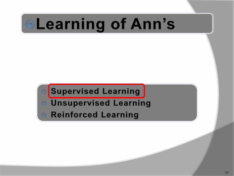
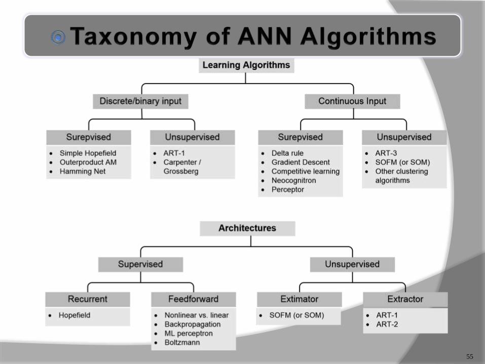
Learning of ANN’s

Type of Neural Network

Neural Network Architecture

Basic of Neural Network

Introduction

Logistic Structure

Model Building

Development of ANN Model

Example

3

4

ANN (Artificial Neural Networks) and SVM

(Support Vector Machines) are two popular

strategies for classification.

They are well-suited for continuous-valued

inputs and outputs, unlike most

decision tree algorithms.

Neural network algorithms are inherently

parallel; parallelization techniques can be

used to speed up the computation process.

These factors contribute toward the

usefulness of neural networks for

classification and prediction in data mining.

5

An Artificial Neural Network (ANN) is an information processing paradigm that is inspired by biological nervous systems.

It is composed of a large number of highly interconnected processing elements called neurons.

An ANN is configured for a specific application, such as pattern recognition or data classification

6

Ability to derive meaning from

complicated or imprecise data

Extract patterns and detect trends that

are too complex to be noticed by either

humans or other computer techniques

Adaptive learning

Real Time Operation

7

Conventional computers use an

algorithmic approach.

But neural networks works similar to

human brain and learns by example.

8

9

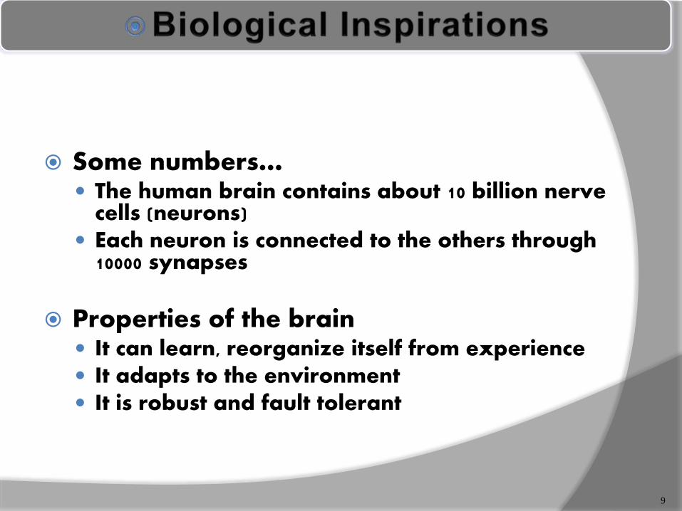
Some numbers… The human brain contains about 10 billion nerve

cells (neurons) Each neuron is connected to the others through

10000 synapses

Properties of the brain It can learn, reorganize itself from experience It adapts to the environment It is robust and fault tolerant

10

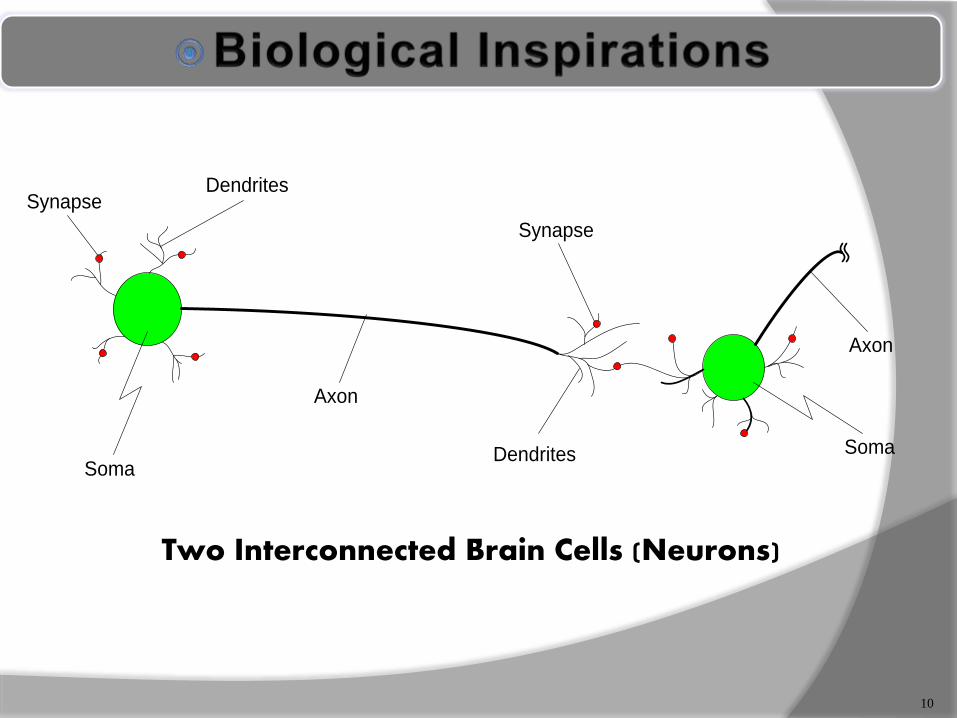
Soma

Axon

Axon

Synapse

SynapseDendrites

Dendrites Soma

Two Interconnected Brain Cells (Neurons)

11

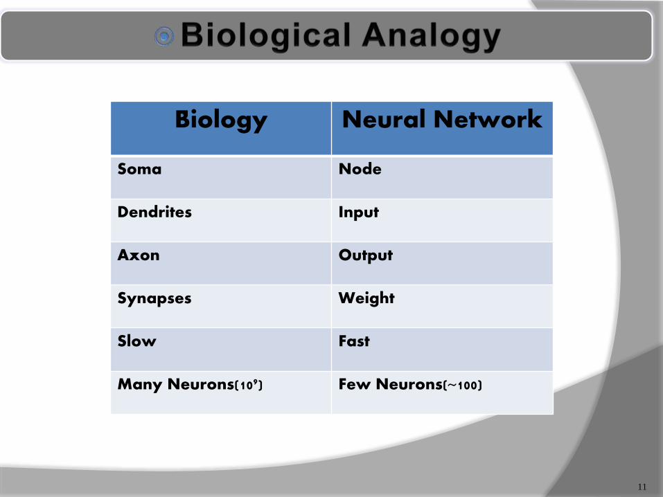
Biology Neural Network

Soma Node

Dendrites Input

Axon Output

Synapses Weight

Slow Fast

Many Neurons(109) Few Neurons(~100)

12

w1

w2

wn

x1

x2

xn

.

.

.

Y

Y1

Yn

Y2

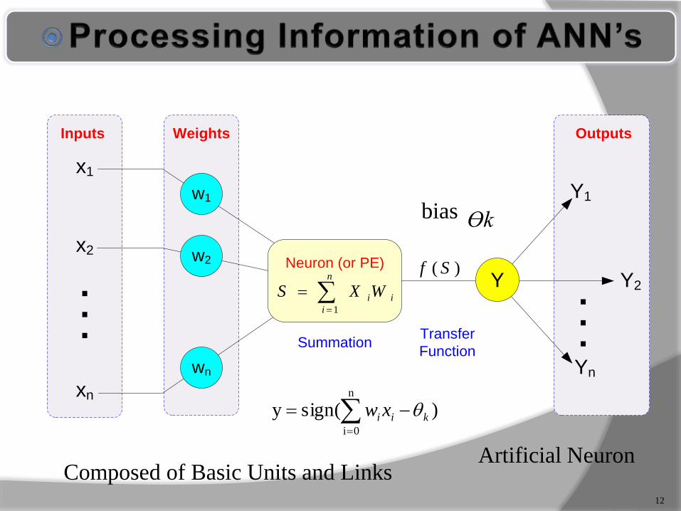
Inputs Weights Outputs

.

.

.

Neuron (or PE)

n

i

iiWXS1

)( Sf

SummationTransfer

Function

bias

Artificial Neuron

)sign(yn

0i

kii xw

Ɵk

Composed of Basic Units and Links

13

Processing element (PE)

Network architecture

Hidden layers

Parallel processing

Network information processing

Inputs

Outputs

Connection weights

Summation function

14

The following are the basic characteristics of neural network:• Exhibit mapping capabilities, they can map

input patterns to their associated output patterns

• Learn by examples

• Robust

• system and fault tolerant

• Process the capability to generalize. Thus, they can predict new outcomes from past trends

15

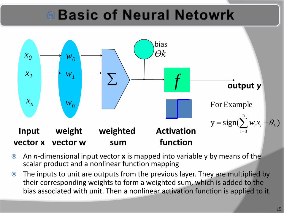
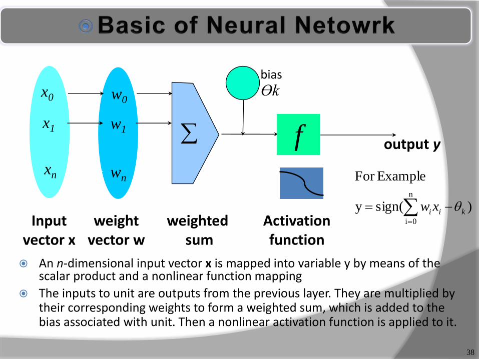
An n-dimensional input vector x is mapped into variable y by means of the scalar product and a nonlinear function mapping

The inputs to unit are outputs from the previous layer. They are multiplied by their corresponding weights to form a weighted sum, which is added to the bias associated with unit. Then a nonlinear activation function is applied to it.

Ɵk

f

weighted sum

Inputvector x

output y

Activationfunction

weightvector w

w0

w1

wn

x0

x1

xn

)sign(y

ExampleFor

n

0i

kii xw

bias

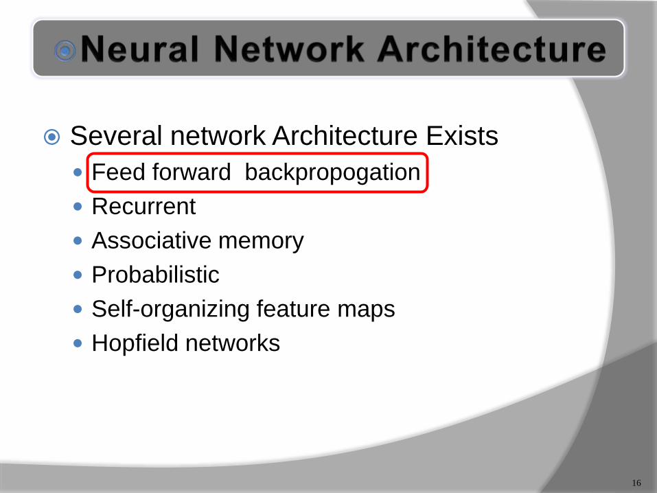
Several network Architecture Exists

Feed forward backpropogation

Recurrent

Associative memory

Probabilistic

Self-organizing feature maps

Hopfield networks

16

In a feed forward network, information

flows in one direction along connecting

pathways, from the input layer via

hidden layers to the final output layer.

There is not feedback, the output of any

layers of any layer does not affect that

same or preceding layer.

17

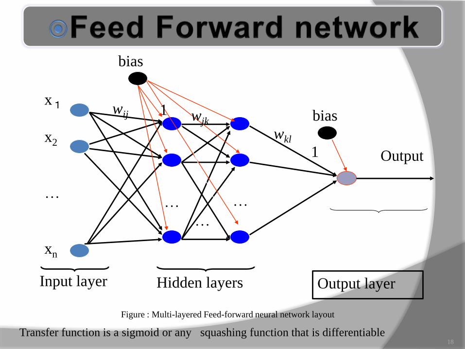
Output

x１

x2

…

xn

bias

biaswij

Input layer Hidden layers Output layer

…

… …

wjk

wkl

Transfer function is a sigmoid or any squashing function that is differentiable

1

1

Figure : Multi-layered Feed-forward neural network layout

18

How can I design the topology of the neural network?

Before training can begin, the usermust decide on the network topology by specifying the number of units in the input layer, the number of hidden layers (if more than one), the number of units in each hidden layer, and the number of units in the output layer.

19

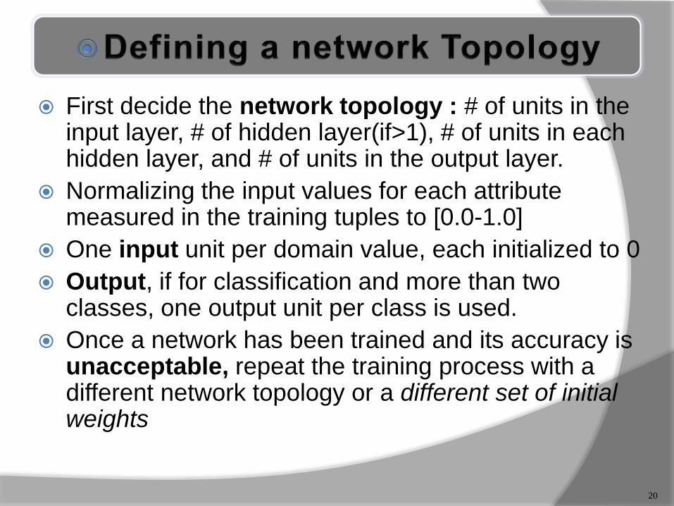
First decide the network topology : # of units in the input layer, # of hidden layer(if>1), # of units in each hidden layer, and # of units in the output layer.

Normalizing the input values for each attribute measured in the training tuples to [0.0-1.0]

One input unit per domain value, each initialized to 0

Output, if for classification and more than two classes, one output unit per class is used.

Once a network has been trained and its accuracy is unacceptable, repeat the training process with a different network topology or a different set of initial weights

20

Number of Hidden Layers

Number of Hidden Nodes

Number of output Nodes

21

22

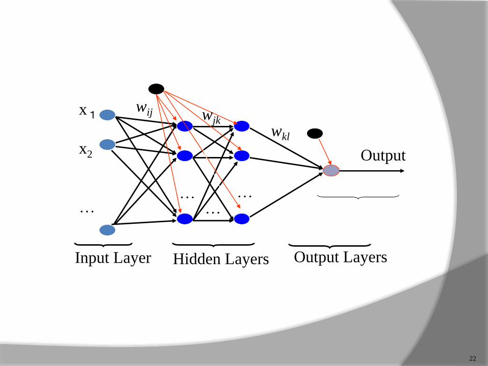
Output

x１

x2

…

wij

Input Layer Hidden Layers

…… …

wjk

wkl

Output Layers

Back Propagation described by Arthur E.

Bryson and Yu-Chi Ho in 1969, but it

wasn't until 1986, through the work of

David E. Rumelhart, Geoffrey E. Hinton

and Ronald J. Williams , that it gained

recognition, and it led to a “renaissance”

in the field of artificial neural network

research.

The term is an abbreviation for & quot;

backwards propagation of errors & quot;.

23

Iteratively process a set of training tuples & compare the

network's prediction with the actual known target value

For each training tuple, the weights are modified to minimize the

mean squared error between the network's prediction and the

actual target value

From a statistical point of view, networks perform nonlinear

regression

Modifications are made in the “backwards” direction: from the

output layer, through each hidden layer down to the first hidden

layer, hence “backpropagation”

Steps

Initialize weights (to small random #s) and biases in the network

Propagate the inputs forward (by applying activation function)

Backpropagate the error (by updating weights and biases)

Terminating condition (when error is very small, etc.)24

FEED FORWARD NETWORK activation

flows in one direction only: from the

input layer to the output layer, passing

through the hidden layer.

Each unit in a layer is connected in the

forward direction to every unit in the next

layer.

25

Several Nerual Network Types Is

Multi Layer Perception

Radial Base Function

Kohenen Self Organizing Feature

26

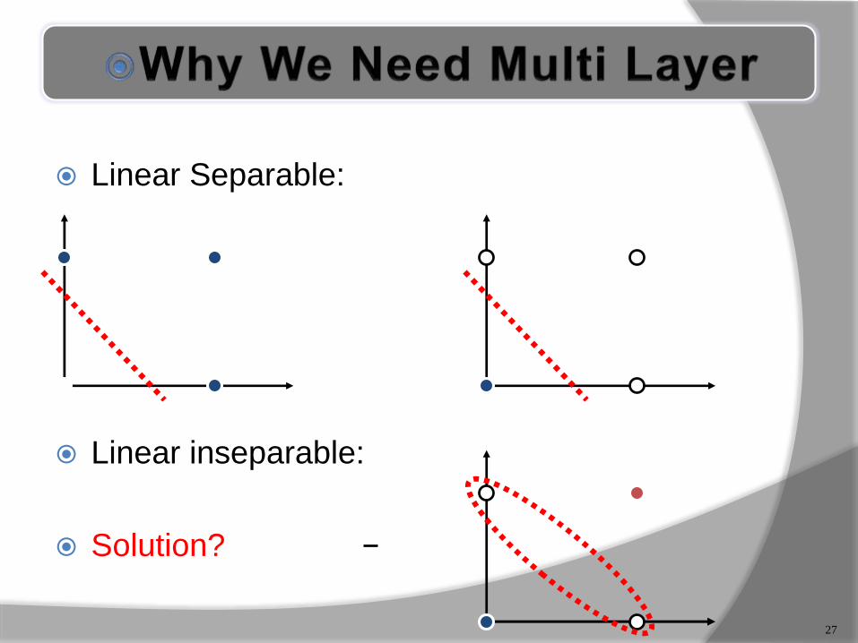
Linear Separable:

Linear inseparable:

Solution?

yx yx

yx

27

Back propagation is a multilayer feed forward network with one layer of z-hidden units.

The y output units has b(i) bias and Z-hidden unit has b(h) as bias. It is found that both the output and hidden units have bias. The bias acts like weights on connection from units whose output is always 1.

The input layer is connected to the hidden layer and output layer is connected to the output layer by means of interconnection weights.

28

The architecture of back propagation resembles a multi-layered feed forward network.

The increasing the number of hidden layers results in the computational complexity of the network.

As a result, the time taken for convergence and to minimize the error may be very high.

The bias is provided for both the hidden and the output layer, to act upon the net input to be calculated.

29

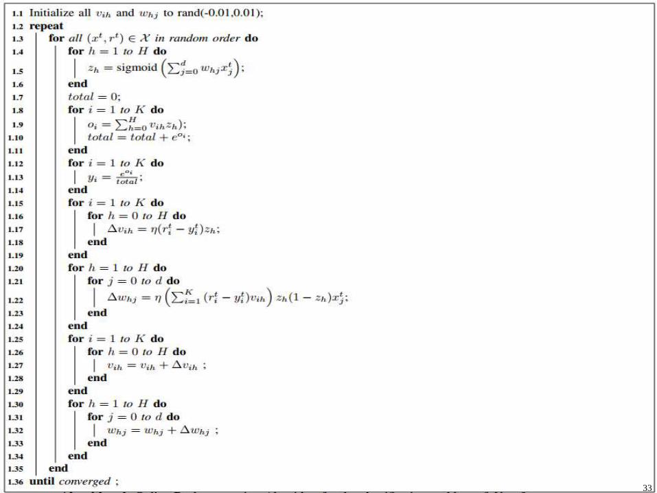
The training algorithm of back propagation involves four stages.

Initialization of weights- some small random values are

assigned.

Feed forward- each input unit (X) receives an input signal and

transmits this signal to each of the hidden units Z 1 ,Z 2 ,……Zn

Each hidden unit then calculates the activation function and

sends its signal Z i to each output unit. The output unit

calculates the activation function to form the response of the

given input pattern.

Back propagation of errors- each output unit compares

activation Y k with its target value T K to determine the

associated error for that unit. Based on the error, the factor δ O

(O=1,……,m) is computed and is used to distribute the error at

output unit Y k back to all units in the previous layer. Similarly,

the factor δ H (H=1,….,p) is compared for each hidden unit H j.

Updating of the weights and biases

30

31

32

Mr.Khan 3333

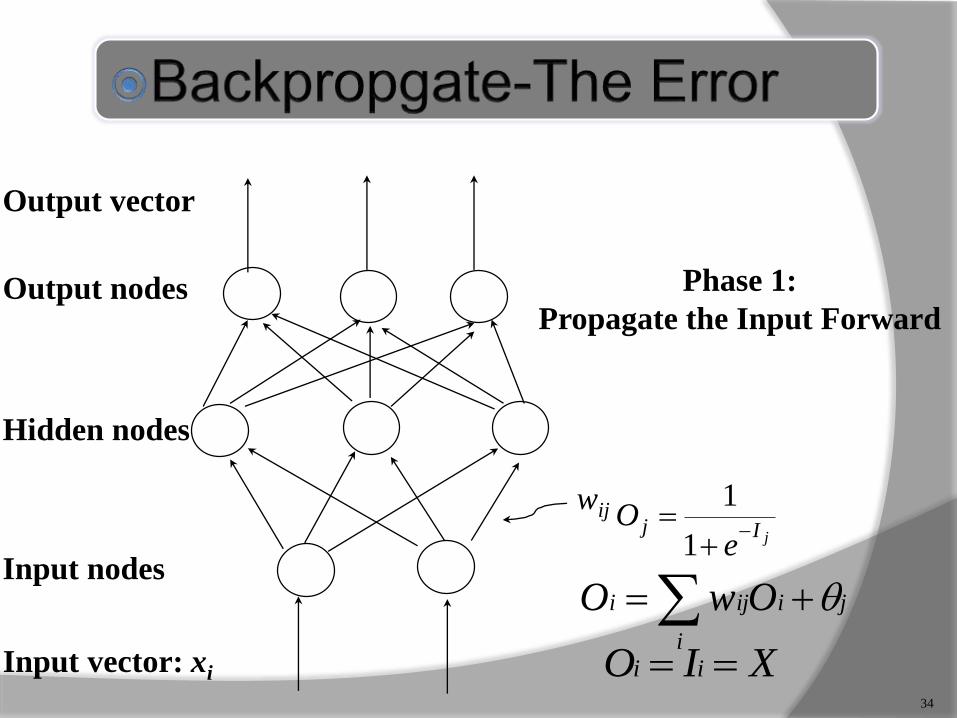
Output nodes

Input nodes

Hidden nodes

Output vector

Input vector: xi

wij

jIje

O

1

1

34

XIO ii

ji

i

iji OwO

Phase 1:

Propagate the Input Forward

Output nodes

Input nodes

Hidden nodes

Output vector

Input vector: xi

wij

))(1( jjjjj OTOOErr

jkk

kjjj wErrOOErr )1(

35

Phase 2:

Back propagate the Error

Output nodes

Input nodes

Hidden nodes

Output vector

Input vector: xi

Oj

36

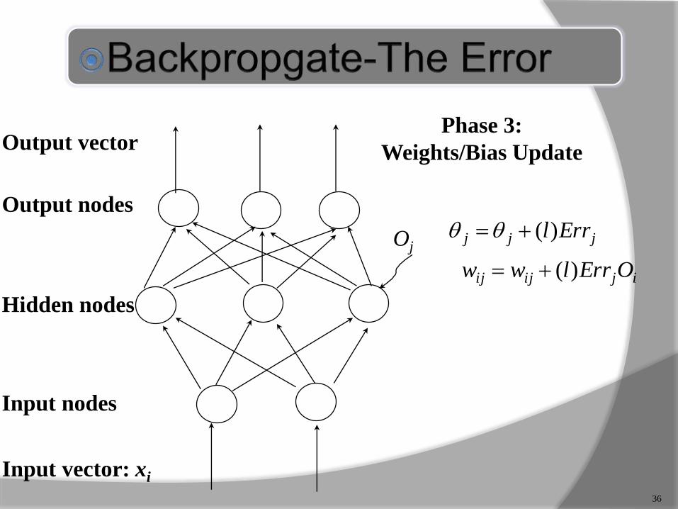
ijijij OErrlww )(

jjj Errl)(

Phase 3:

Weights/Bias Update

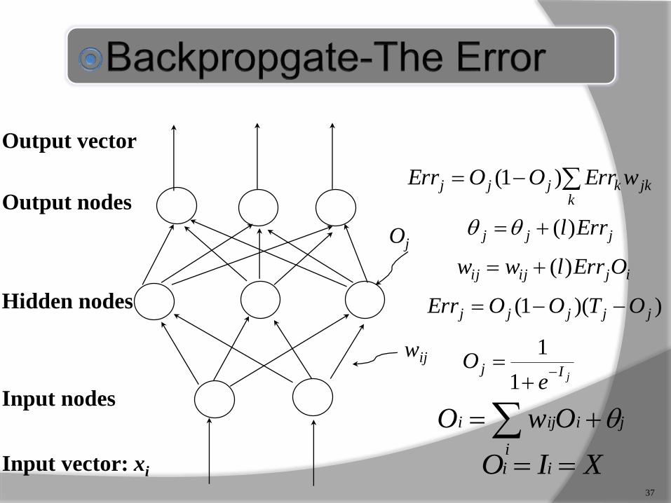
Output nodes

Input nodes

Hidden nodes

Output vector

Input vector: xi

wij

jIje

O

1

1

))(1( jjjjj OTOOErr

jkk

kjjj wErrOOErr )1(

ijijij OErrlww )(

jjj Errl)(

37

XIO ii

ji

i

iji OwO

Oj

38

An n-dimensional input vector x is mapped into variable y by means of the scalar product and a nonlinear function mapping

The inputs to unit are outputs from the previous layer. They are multiplied by their corresponding weights to form a weighted sum, which is added to the bias associated with unit. Then a nonlinear activation function is applied to it.

Ɵk

f

weighted sum

Inputvector x

output y

Activationfunction

weightvector w

w0

w1

wn

x0

x1

xn

)sign(y

ExampleFor

n

0i

kii xw

bias

The inputs to the network correspond to the attributes measured for each training tuple.

Inputs are fed simultaneously into the units making up the input layer.

They are then weighted and fed simultaneously to a hidden layer

The number of hidden layers is arbitrary, although usually only one

The weighted outputs of the last hidden layer are input to units making up the output layer, which emits the network's prediction

The network is feed-forward in that none of the weights cycles back to an input unit or to an output unit of a previous layer

39

40

41

42

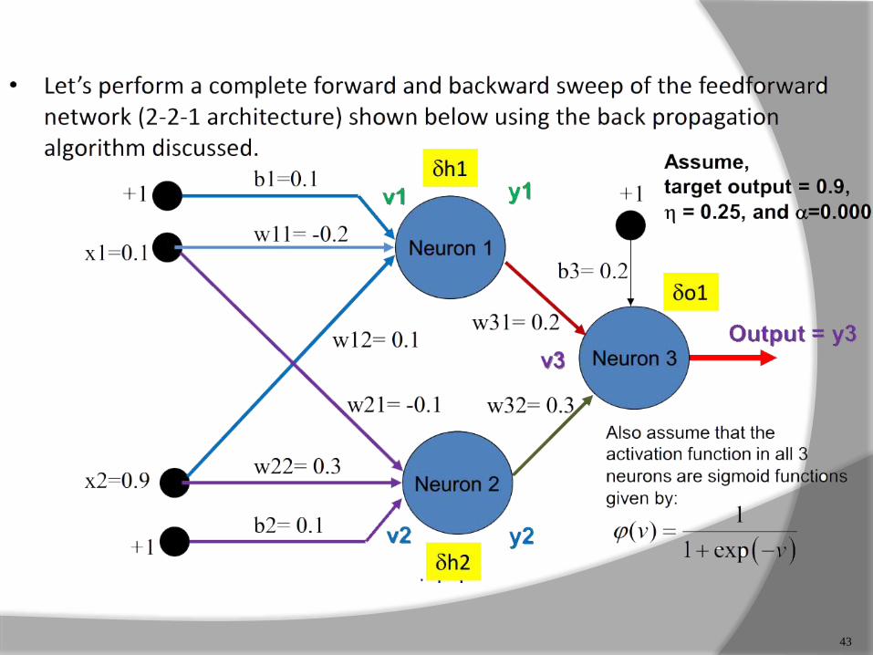
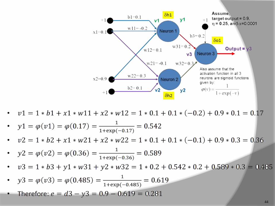
43

44

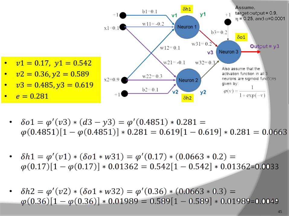
45

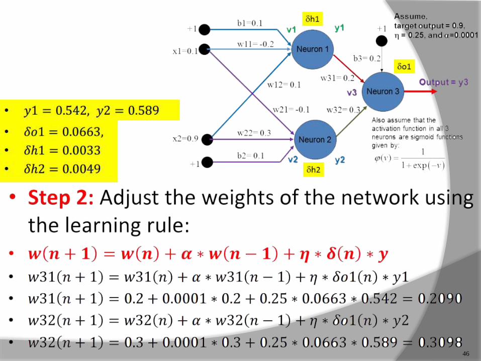
46

47

48

49

50

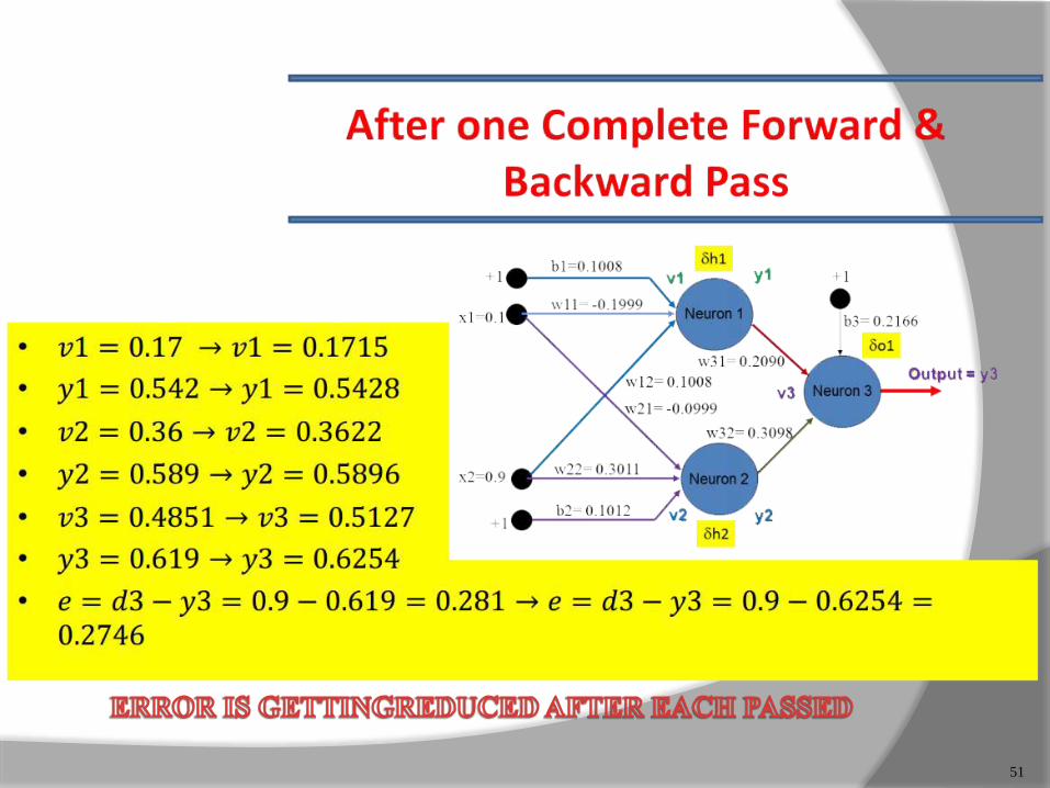
51

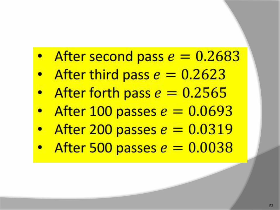
52

53

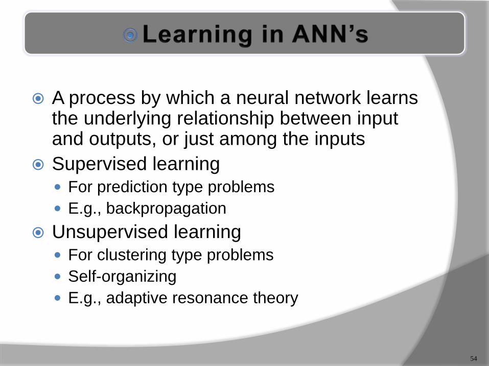
A process by which a neural network learns the underlying relationship between input and outputs, or just among the inputs

Supervised learning For prediction type problems

E.g., backpropagation

Unsupervised learning For clustering type problems

Self-organizing

E.g., adaptive resonance theory

54

55

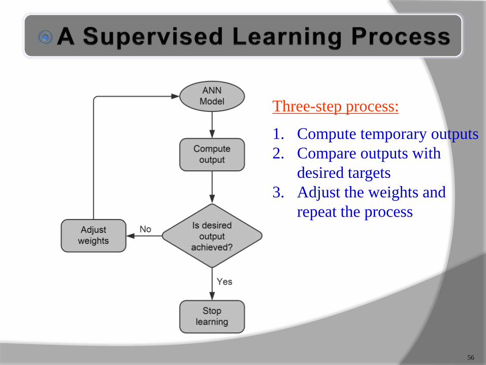
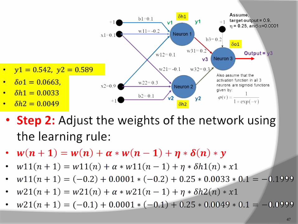
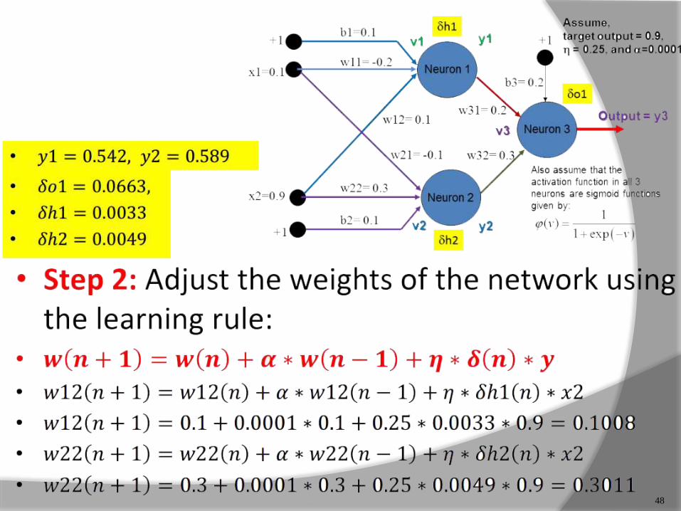
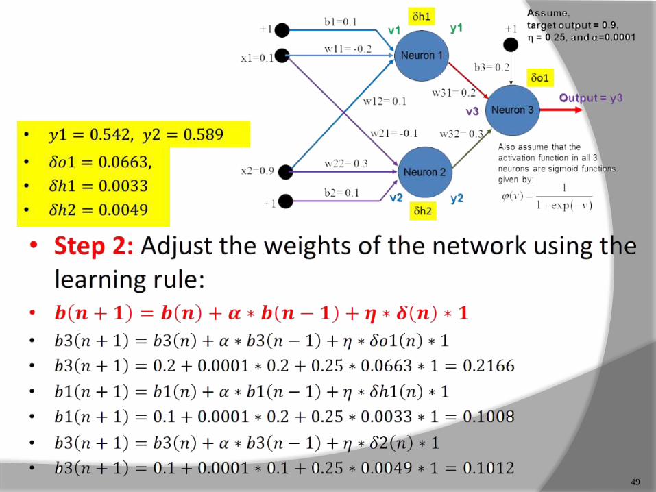
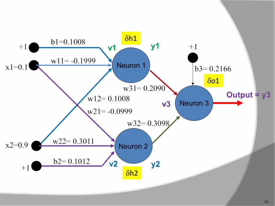
Three-step process:

1. Compute temporary outputs

2. Compare outputs with

desired targets

3. Adjust the weights and

repeat the process

56

57

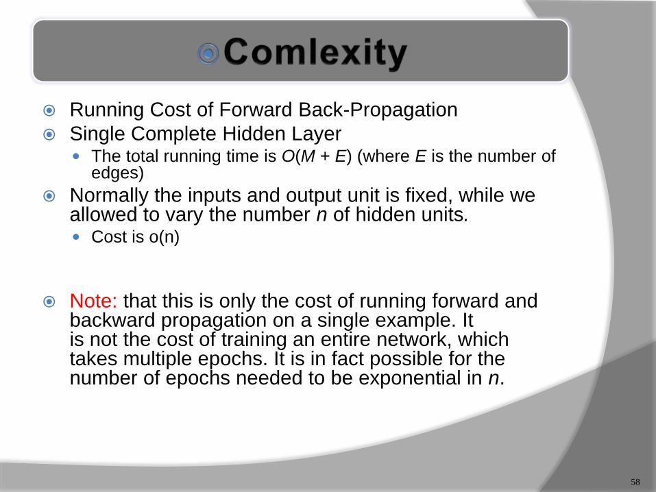
Running Cost of Forward Back-Propagation

Single Complete Hidden Layer The total running time is O(M + E) (where E is the number of

edges)

Normally the inputs and output unit is fixed, while we allowed to vary the number n of hidden units. Cost is o(n)

Note: that this is only the cost of running forward and backward propagation on a single example. Itis not the cost of training an entire network, which takes multiple epochs. It is in fact possible for the number of epochs needed to be exponential in n.

58

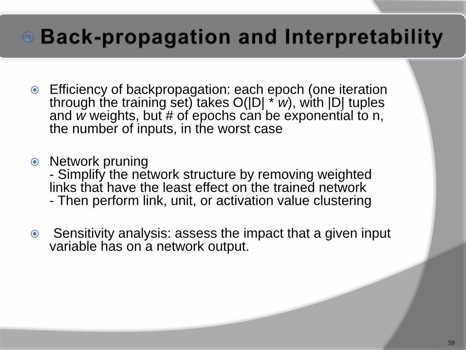
Efficiency of backpropagation: each epoch (one iteration through the training set) takes O(|D| * w), with |D| tuplesand w weights, but # of epochs can be exponential to n, the number of inputs, in the worst case

Network pruning- Simplify the network structure by removing weighted links that have the least effect on the trained network- Then perform link, unit, or activation value clustering

Sensitivity analysis: assess the impact that a given input variable has on a network output.

59

60

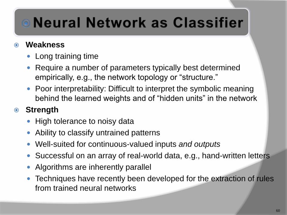
Weakness

Long training time

Require a number of parameters typically best determined

empirically, e.g., the network topology or “structure.”

Poor interpretability: Difficult to interpret the symbolic meaning

behind the learned weights and of “hidden units” in the network

Strength

High tolerance to noisy data

Ability to classify untrained patterns

Well-suited for continuous-valued inputs and outputs

Successful on an array of real-world data, e.g., hand-written letters

Algorithms are inherently parallel

Techniques have recently been developed for the extraction of rules

from trained neural networks

In this question, I'd like to know specifically what aspects of an ANN

(specifically, a Multilayer Perceptron) might make it desirable to use over

an SVM? The reason I ask is because it's easy to answer

the opposite question: Support Vector Machines are often superior to

ANNs because they avoid two major weaknesses of ANNs:

(1) ANNs often converge on local minima rather than global minima,

meaning that they are essentially "missing the big picture" sometimes (or

missing the forest for the trees)

(2) ANNs often overfit if training goes on too long, meaning that for any

given pattern, an ANN might start to consider the noise as part of the

pattern.

SVMs don't suffer from either of these two problems. However, it's not

readily apparent that SVMs are meant to be a total replacement for ANNs.

So what specific advantage(s) does an ANN have over an SVM that might

make it applicable for certain situations? I've listed specific advantages of

an SVM over an ANN, now I'd like to see a list of ANN advantages

61

Activation function - A mathematical function applied to a node’s

activation that computes the signal strength it outputs to

subsequent nodes.

Activation - The combined sum of a node’s incoming, weighted

signals.

Backpropagation - A supervised learning algorithm which uses

data with associated target output to train an ANN.

Connections - The paths signals follow between ANN nodes.

Connection weights - Signals passing through a connection are

multiplied by that connection’s weight.

Dataset - See Input pattern

Epoch - One iteration through the backpropagation algorithm

(presentation of the entire training set once to the network).

Feedforward ANN - An ANN architecture where signal flow is in

one direction only.

62

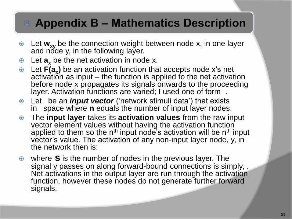
Let wxy be the connection weight between node x, in one layer and node y, in the following layer.

Let ax be the net activation in node x.

Let F(ax) be an activation function that accepts node x’s net activation as input – the function is applied to the net activation before node x propagates its signals onwards to the proceeding layer. Activation functions are varied; I used one of form .

Let be an input vector (‘network stimuli data’) that exists in space where n equals the number of input layer nodes.

The input layer takes its activation values from the raw input vector element values without having the activation function applied to them so the nth input node’s activation will be nth input vector’s value. The activation of any non-input layer node, y, in the network then is:

where s is the number of nodes in the previous layer. The signal y passes on along forward-bound connections is simply, . Net activations in the output layer are run through the activation function, however these nodes do not generate further forward signals.

63

Generalization - A well trained ANN’s ability to correctly classify unseen

input patterns by finding their similarities with training set patterns

Input vector - See Input pattern

Input pattern - An ANN’s input – there may be no pattern, per se. The

pattern has as many elements as the network has input layer nodes.

Maximum training error - Criteria for deciding when to stop training an

ANN.

Network architecture - The design of an ANN: the number of units and

their pattern of connection.

Output - The signal a node passes on to subsequent layers (before

being multiplied by a connection weight). In the output layer, the set of

each node’s output is the ANN’s output for a particular input vector.

Training - Process allowing an ANN to learn.

Training set - The set of input patterns used during network training.

Each input pattern has an associated target output.

Weights - See Connection weights.

64

65