MULTI-CRITERIA OPTIMISATION OF GROUP REPLACEMENT SCHEDULES FOR DISTRIBUTED WATER PIPELINE ASSETS Fengfeng Li Bachelor of Engineering (Mechanical) Master of Engineering (Mechanical) Submitted in partial fulfilment of the requirements for the degree of Doctor of Philosophy School of Chemistry, Physics and Mechanical Engineering Science and Engineering Faculty Queensland University of Technology 2013

Welcome message from author
This document is posted to help you gain knowledge. Please leave a comment to let me know what you think about it! Share it to your friends and learn new things together.
Transcript

MULTI-CRITERIA OPTIMISATION OF GROUP REPLACEMENT SCHEDULES FOR DISTRIBUTED WATER PIPELINE ASSETS
Fengfeng Li Bachelor of Engineering (Mechanical) Master of Engineering (Mechanical)
Submitted in partial fulfilment of the requirements for the degree of
Doctor of Philosophy
School of Chemistry, Physics and Mechanical Engineering
Science and Engineering Faculty
Queensland University of Technology
2013


Multi-criteria Optimisation of Maintenance Schedules for Distributed Water Pipeline Assets i
Keywords
Reliability Analysis, Hazard Models, Multi-Criteria Optimisation, Pipeline Maintenance, Decision Support, Cost Modelling, Service Interruption Modelling, Group Replacement Scheduling

ii Multi-criteria Optimisation of Maintenance Schedules for Distributed Water Pipeline Assets

Multi-criteria Optimisation of Maintenance Schedules for Distributed Water Pipeline Assets iii
Abstract
Pipes in underground water distribution systems deteriorate over time. Replacement
of deteriorated water pipes is often a capital-intensive decision for utility companies.
Replacement planning aims to minimise total costs while maintaining a satisfactory
level of services.
This candidature presents an optimization model for group replacement schedules of
water pipelines. Throughout this thesis this model is referred to as RDOM-GS, i.e.,
Replacement Decision Optimisation Model for Group Scheduling. This
candidature also presents an improved hazard modelling method for predicting the
reliability of water pipelines, which can be applied to calculate the total costs and
total service interruptions in RDOM-GS. These new models and methodology are
designed to improve the accuracy of reliability prediction and provide a new
approach to optimising schedules for replacement of groups of water pipelines.
A comprehensive literature review covering the reliability analysis and replacement
optimisation of water pipes has revealed the following limitations of the current
state-of-the-art: (1) In practice, replacement of water pipelines is usually scheduled
into groups based on expert experience in order to reduce maintenance costs.
However, existing research on water pipe replacement optimisation focuses on
individual pipes. (2) Pipe networks are a mix of different pipe materials, diameters,
length and other operating environmental conditions. However, an effective approach
to statistical grouping has not yet been developed in the reliability analyses for water
pipes.
RDOM-GS optimises replacement schedules by considering three group-scheduling
criteria: shortest geographic distance, maximum replacement equipment utilization,
and minimum service interruption. In order to be able to reach an optimal
replacement solution considering group scheduling, a modified evolutionary
optimisation algorithm was developed in this thesis and integrated with the
RDOM-GS. By integrating new cost functions, a model of service interruption, and
optimisation algorithms into a unified procedure, RDOM-GS is able to deliver
iv Multi-criteria Optimisation of Maintenance Schedules for Distributed Water Pipeline Assets
replacement schedules minimising total life-cycle cost, and conditionally keeping
service interruptions under a specified limit.
The proposed improved hazard modelling method for water pipes has three
improvements on existing methods: (1) it can systematically partition water pipeline
data into relatively homogeneous statistical groups through developing a statistical
grouping algorithm; (2) it can reduce the underestimation effects caused by real life
data through developing a modified empirical hazard model; (3) it can differentiate
the application impacts of two commonly used empirical hazard formulas through a
comparative study. This candidature proposes a Monte Carlo simulation framework
of water pipelines to generate test-bed sample data sets that characterises primary
features of the real-world data. The framework enables the evaluation the hazard
modelling method for censored data.
These newly developed methodologies/models have been verified using simulations
and industrial case studies. The results of the industrial case study show that the
methodologies and models proposed in this candidature can effectively improve
replacement planning of water pipes by considering multi-criteria group scheduling.
Also, total life-cycle costs can be reduced by 5%, as well as a reduction by 11.25%
on service interruptions.
The research outcomes of this candidature are expected to enrich the body of
knowledge in the field of optimal replacement of water pipes, where group
scheduling based on multiple criteria is considered in water-pipe replacement
decisions. RDOM-GS combined with cost analysis, service interruption analysis and
optimisation analysis is able to deliver optimised replacement schedules in order to
reduce investment costs and service interruptions. Additionally, by applying the
improved hazard modelling method, water pipeline data can systematically be
grouped by their specific features, so that the accuracy of reliability analysis
considering pipe segments can be enhanced.

Multi-criteria Optimisation of Maintenance Schedules for Distributed Water Pipeline Assets v
Table of Contents
Keywords .................................................................................................................................................. i Abstract .................................................................................................................................................. iii Table of Contents .................................................................................................................................... v List of Figures ........................................................................................................................................ ix List of Tables .......................................................................................................................................... xi Nomenclature ....................................................................................................................................... xiii Statement of Original Authorship ........................................................................................................ xix Acknowledgements ............................................................................................................................... xx CHAPTER 1: INTRODUCTION ....................................................................................................... 1 1.1 Introduction of research ................................................................................................................. 1 1.2 Research Objectives ...................................................................................................................... 3 1.3 Research methods .......................................................................................................................... 6 1.4 Outcomes of the research ............................................................................................................ 10 1.5 Originality and innovation ........................................................................................................... 12 1.6 Research Procedures .................................................................................................................... 15 1.7 Publications Generated from This Research ............................................................................... 16 1.8 Some Important Definitions ........................................................................................................ 17 1.9 Thesis Outline .............................................................................................................................. 19 CHAPTER 2: LITERATURE REVIEW ......................................................................................... 23 2.1 Water Pipe Failures ..................................................................................................................... 23
2.1.1 Consequences of water pipe failures ................................................................................... 23 2.1.2 Failure modes of water pipe ................................................................................................. 24 2.1.3 Replacement cost on water pipes ......................................................................................... 26
2.2 Reliability Analysis for Water Pipe Networks ............................................................................ 27 2.3 Maintenance Decision Making for Water Pipe Network ............................................................ 29
2.3.1 Maintenance strategy ........................................................................................................... 29 2.3.2 Replacement decision making for water pipe network ........................................................ 31
2.4 Evolutionary Algorithms for Multi-objective Optimization ....................................................... 35 2.5 Concluding Remarks ................................................................................................................... 40 CHAPTER 3: IMPROVED HAZARD BASED MODELLING METHOD ................................. 43 3.1 Introduction ................................................................................................................................. 43 3.2 The Discrete Hazard Based Modelling Method for Linear Assets .............................................. 45
3.2.1 Piece-wise hazard model for linear asset ............................................................................. 45 3.2.2 Assumptions of the piece-wise hazard model ...................................................................... 49
3.3 Statistical Grouping Algorithm for Hazard Modelling ................................................................ 49 3.3.1 Statistical grouping algorithm based on regression tree ...................................................... 50

vi Multi-criteria Optimisation of Maintenance Schedules for Distributed Water Pipeline Assets
3.3.2 A case study to test the proposed statistical grouping algorithm ......................................... 54 3.4 Theoretic Formulas of Empirical Hazards, and Evaluation ........................................................ 60
3.4.1 Introduction of empirical hazard function ........................................................................... 60 3.4.2 Empirical hazard function derivation and discussion .......................................................... 62 3.4.3 Comparison of empirical hazard function formulas using simulation samples ................... 66
3.5 Hazard Modelling for Truncated Lifetime Data of Water Pipes ................................................. 69 3.5.1 The real situation of lifetime data for water pipes ............................................................... 69 3.5.2 Empirical hazard function for interval truncated lifetime data ............................................ 72 3.5.3 Monte Carlo simulation based on real lifetime data for water pipes ................................... 73 3.5.4 Validation of the proposed empirical hazard function ......................................................... 74 3.5.5 Hazard distribution fitting method for the piece-wise hazard model .................................. 81
3.6 Procedure of the improved Hazard Modelling method for Water Pipes ..................................... 82 3.7 Summary ...................................................................................................................................... 83 CHAPTER 4: OPTIMIZATION MODEL OF GROUP REPLACEMENT SCHEDULES FOR WATER PIPELINES .......................................................................................................................... 85 4.1 Introduction ................................................................................................................................. 85 4.2 Maintenance on Water Pipelines ................................................................................................. 86
4.2.1 Repair and replacement of water pipeline ........................................................................... 86 4.2.2 Economics of pipeline failure and pipeline replacement ..................................................... 87
4.3 Cost Functions for Water Pipeline Replacement Planning ......................................................... 89 4.3.1 Age specified cost functions of water pipeline failure ........................................................ 89 4.3.2 Function of total cost in a planning period T ....................................................................... 90
4.4 Replacement Group Scheduling .................................................................................................. 94 4.4.1 Criteria of the replacement group scheduling ...................................................................... 94 4.4.2 Judgment matrix .................................................................................................................. 96 4.4.3 The calculation of geographical distance ............................................................................. 96 4.4.4 Determination of equipment utilization ............................................................................... 97 4.4.5 Service interruption for group scheduling criteria ............................................................... 97
4.5 Group Scheduling Based Replacement Cost Function ................................................................ 98 4.6 Impact of Service Interruption ................................................................................................... 100 4.7 Objectives and Constrains for the RDOM-GS .......................................................................... 101 4.8 Structure of the RDOM-GS for Water Pipelines ....................................................................... 103 4.9 Summary .................................................................................................................................... 105 CHAPTER 5: AN IMPROVED MULTI-OBJECTIVE OPTIMISATION ALGORITHM FOR GROUP SCHEDULING ................................................................................................................... 107 5.1 Introduction ............................................................................................................................... 107 5.2 Group Scheduling Optimisation Problem (GSOP) .................................................................... 107 5.3 Procedure of the Modified NSGA-II ......................................................................................... 109 5.4 Operators of the Modified NSGA-II ......................................................................................... 111
5.4.1 Encoding method ............................................................................................................... 111 5.4.2 Initialization operator ......................................................................................................... 113

Multi-criteria Optimisation of Maintenance Schedules for Distributed Water Pipeline Assets vii
5.4.3 Crossover operator ............................................................................................................. 113 5.4.4 Mutation operator .............................................................................................................. 113 5.4.5 Crowding distance operator ............................................................................................... 115 5.4.6 Selection Operator ............................................................................................................. 117
5.5 Comparative Study .................................................................................................................... 118 5.5.1 Simplified objective functions ........................................................................................... 118 5.5.2 Parameter settings .............................................................................................................. 118 5.5.3 Results comparison ............................................................................................................ 119
5.6 Summary .................................................................................................................................... 121 CHAPTER 6: A CASE STUDY ...................................................................................................... 123 6.1 Introduction ............................................................................................................................... 123 6.2 Data Pre-analysis ....................................................................................................................... 124
6.2.1 Overview of the water pipeline network ............................................................................ 124 6.2.2 Age Profile of the Water Pipeline Network ....................................................................... 124 6.2.3 Repair history of water pipe ............................................................................................... 128 6.2.4 Repair history of service interruption ................................................................................ 131
6.3 Hazard Calculation and Prediction ............................................................................................ 131 6.3.1 Statistical grouping analysis .............................................................................................. 131 6.3.2 Empirical hazards for each group ...................................................................................... 133 6.3.3 Predicted number of failures for each group ..................................................................... 136
6.4 Replacement Decision Optimisation for Group Scheduling ..................................................... 140 6.4.1 Parameters for cost function and service interruption ....................................................... 140 6.4.2 Judgment matrix ................................................................................................................ 143 6.4.3 Parameters for the modified NSGA-II ............................................................................... 145 6.4.4 Results and discussions ...................................................................................................... 145
6.5 Discussions ................................................................................................................................ 148 CHAPTER 7: CONCLUSIONS AND FUTURE WORK ............................................................. 151 7.1 SUMmary OF RESEARCH ...................................................................................................... 152 7.2 Research Contributions .............................................................................................................. 153
7.2.1 Multi-objective multi-criteria optimisation for group replacement schedules .................. 153 7.2.2 Improved Hazard modelling methods for water pipelines ................................................. 155 7.2.3 Application of the proposed models in a real case study ................................................... 156
7.3 Future Research Directions ....................................................................................................... 157 7.3.1 Extension of multi-objective RDOM-GS .......................................................................... 157 7.3.2 Extension of hazard modelling method for water pipes .................................................... 157 7.3.3 Application to other linear assets ....................................................................................... 158
7.4 Final remarks ............................................................................................................................. 158 BIBLIOGRAPHY ............................................................................................................................. 161

viii Multi-criteria Optimisation of Maintenance Schedules for Distributed Water Pipeline Assets

Multi-criteria Optimisation of Maintenance Schedules for Distributed Water Pipeline Assets ix
List of Figures
Figure 1-1 Stage 1 and Stage 2 ................................................................................................................ 7 Figure 1-3 Research procedures ............................................................................................................ 16 Figure 3-1 Sketch of water pipe segmentation ...................................................................................... 44 Figure 3-3 Typical two-phase failure pattern for linear assets .............................................................. 46 Figure 3-4 PDF, CDF, reliability and hazard function of the piecewise hazard model ........................ 48 Figure 3-5 Regression tree structure ..................................................................................................... 51 Figure 3-6 Procedure of the proposed statistical grouping algorithm ................................................... 53 Figure 3-7 Relationship between failures/100m and average age for each material type ..................... 56 Figure 3-8 Regression tree for grouping of all pipes except MS pipes ................................................. 56 Figure 3-9 Regression tree of grouping for pipe length greater than one metre except MS pipes ........ 57 Figure 3-10 Empirical hazard and smoothed line patterns (Excluding Group 6) ................................. 59 Figure 3-11 Empirical hazard and smoothed line patterns (excluding Group 5 and Group 6) ............. 59 Figure 3-12 Investigation of the bias effects of the empirical hazard function values calculated
using h1! and h2! ............................................................................................................. 65 Figure 3-13 Empirical hazard function values calculated using h1! (the top and third panel
plots) and h2! (the second and bottom panel plots) ........................................................... 67 Figure 3-14 Empirical hazard function values calculated using h1! (top panel plot) and h2!
(bottom panel plot) ............................................................................................................... 68 Figure 3-15 Schematic of lifetime distribution of water pipe segment in calendar time ...................... 70 Figure 3-16 Schematic of lifetime distribution of water pipes (age-specific) ....................................... 71 Figure 3-17 The goodness-of-fit of empirical hazards vs. the true hazard based on Equation
(3-18) .................................................................................................................................... 75 Figure 3-18 The goodness-of-fit of empirical hazards vs. the true hazard based on Equation
(3-19) .................................................................................................................................... 76 Figure 3-19 The goodness-of-fit of empirical hazards vs. the true hazard in Situation A based
on Equation (3-18) ................................................................................................................ 77 Figure 3-20 The goodness-of-fit of empirical hazards vs. the true hazard in Situation A based
on Equation (3-19) ................................................................................................................ 78 Figure 3-21 The goodness-of-fit of empirical hazards vs. the true hazard in Situation B based
on Equation (3-19) ................................................................................................................ 79 Figure 3-22 The goodness-of-fit of empirical hazards vs. the true hazard based on Equation
(3-18) .................................................................................................................................... 80 Figure 3-23 The goodness-of-fit of empirical hazards vs. the true hazard based on Equation
(3-19) .................................................................................................................................... 80 Figure 3-24 The goodness-of-fit of fitted hazards vs. the empirical hazard based of Example 1 ......... 82 Figure 4-1 Failure cost rate with replacement at τ ............................................................................... 90 Figure 4-2 Repair cost rate during a planning period T ........................................................................ 91 Figure 4-3 Structure of the RDOM-GS ............................................................................................... 103 Figure 5-1 Procedure of the modified NSGA-II ................................................................................. 111

x Multi-criteria Optimisation of Maintenance Schedules for Distributed Water Pipeline Assets
Figure 5-2 Encoding structure ............................................................................................................. 112 Figure 5-3 One example of encoding representation .......................................................................... 112 Figure 5-4 Illustration of the original crowding distance method ....................................................... 116 Figure 5-5 Modified crowding distance .............................................................................................. 117 Figure 5-6 Pareto-fronts of the optimisation results for NSGA-II and the modified NSGA-II .......... 120 Figure 6-1 Length of pipe being installed for each calendar year ....................................................... 125 Figure 6-2 Cumulative length of pipe being installed for each calendar year .................................... 125 Figure 6-3 Total length of pipe by material type ................................................................................. 126 Figure 6-4 Box plot for different material types of diameter .............................................................. 127 Figure 6-5 Box plot for different material types of installation date ................................................... 128 Figure 6-6 Repair history from 2000 to 2010 ...................................................................................... 129 Figure 6-7 Number of breaks by material types .................................................................................. 129 Figure 6-8 Number of breaks per 100km by material types ................................................................ 130 Figure 6-9 Relationship between failures/100m and average age for each material type ................... 132 Figure 6-10 Hazard curve for group 1 ................................................................................................. 134 Figure 6-11Hazard curve for group 2 .................................................................................................. 134 Figure 6-12 Hazard curve for group 3 ................................................................................................. 134 Figure 6-13 Hazard curve for group 4 ................................................................................................. 135 Figure 6-14 Hazard curve for group 5 ................................................................................................. 135 Figure 6-15 Hazard curve for group 6 ................................................................................................. 135 Figure 6-16 Hazard curve for group 7 ................................................................................................. 136 Figure 6-17 Comparison of the fitted hazard curve for each group .................................................... 136 Figure 6-18 Predicted number of failures for group 1 ......................................................................... 137 Figure 6-19 Predicted number of failures for group 2 ......................................................................... 137 Figure 6-20 Predicted number of failures for group 3 ......................................................................... 138 Figure 6-21 Predicted number of failures for group 4 ......................................................................... 138 Figure 6-22 Predicted number of failures for group 5 ......................................................................... 138 Figure 6-23 Predicted number of failures for group 6 ......................................................................... 139 Figure 6-24 Predicted number of failures for group 7 ......................................................................... 139 Figure 6-25 Total number predicted failures for all pipes ................................................................... 139 Figure 6-26 Repair cost by materials .................................................................................................. 141 Figure 6-27 Repair cost by pipe diameter ........................................................................................... 141 Figure 6-28 Judgment matrix .............................................................................................................. 144 Figure 6-29 Pareto-front of optimized solution ................................................................................... 146

Multi-criteria Optimisation of Maintenance Schedules for Distributed Water Pipeline Assets xi
List of Tables
Table 2-1 Categories of water pipe material and abbreviations ............................................................ 25 Table 3-1 Split groups based on the proposed statistical grouping algorithm ...................................... 57 Table 3-2 Parameters for Example 1 ..................................................................................................... 75 Table 3-3 Parameters for Example 2 ..................................................................................................... 77 Table 3-4 Parameters for Example 3 ..................................................................................................... 79 Table 3-5 Parameters estimation for Example 1 ................................................................................... 82 Table 4-1 Machinery utilisation based on materials and diameters ...................................................... 97 Table 6-1 Overview of the water pipeline network ............................................................................. 124 Table 6-2 Summary of pipes based on types of material .................................................................... 130 Table 6-3 Statistical grouping criteria, statistical grouping results and the information for each
group ................................................................................................................................... 132 Table 6-4 Hazard model parameters for each group ........................................................................... 133 Table 6-5 Coefficients for repair cost function Cfail .......................................................................... 142 Table 6-6 Water pipes length related replacement cost ................................................................. 142 Table 6-7 Category-specific Impact Factor ......................................................................................... 143 Table 6-8 Service Interruption Duration ............................................................................................. 143 Table 6-9 Summary of the Selected Replacement Planning Solution ................................................. 146 Table 6-10 Summary of the replacement planning of Solution 1 ....................................................... 147 Table 6-11 Details of the first year replacement planning of Solution 1 ............................................ 147 Table 6-12 Examples of the seventh year replacement planning of Solution 1 .................................. 148

xii Multi-criteria Optimisation of Maintenance Schedules for Distributed Water Pipeline Assets

Multi-criteria Optimisation of Maintenance Schedules for Distributed Water Pipeline Assets xiii
Nomenclature
Abbreviations
AFR Average failure rate
AHP Analytic hierarchy process
ANN Artificial neural network
ANOVA Analysis of variance
AWWA The American Water Works Association
cdf Cumulative distribution function
CIEAM Cooperative Research Centre for Infrastructure and Engineering
Asset Management
CM Corrective maintenance
DSM Distributed Scheduling Model
EA Evolutionary algorithm
GA Genetic algorithm
GSOP Group scheduling optimisation problem
GIS Geographic information system
I-WARP Individual Water Main Renewal Planner
MACROS Multi-objective Automated Construction Resource Optimization
System
MLE Maximum likelihood estimation
MOEA Multi-objective evolutionary algorithm
ME-BMS Multiple-element bridge management system
MOGA Multi-objective genetic algorithm
MTTF Mean Time To Failure
NHPP Non-Homogeneous Poisson Process
NORP100M Number of repairs per 100 metres
NPGA Niched Pareto genetic algorithm
NSGA Non-dominated sorting genetic algorithm
NSGA-II Non-dominated sorting genetic algorithm-II
pdf Probability density function

xiv Multi-criteria Optimisation of Maintenance Schedules for Distributed Water Pipeline Assets
PM Preventative maintenance
PdM Predictive maintenance
RBPM Reliability based preventive maintenance
RDOM-GS Replacement decision optimisation model for group scheduling
ROCOF Rate of failure occurrence
SPEA Strength Pareto Evolutionary Algorithm
TBPM Time based preventive maintenance
TTR Time to replacement

Multi-criteria Optimisation of Maintenance Schedules for Distributed Water Pipeline Assets xv
Notations
Roman Letters
𝑐𝑢𝑟𝑟𝐷 Current date
𝐶!,! Transportation cost of pipe i
𝐶!"#$ Cost incurred due to a pipe segment failure
𝐶!"#$ Cost of replacement of one pipe
𝐶!,!!"! Total cost for replacing pipe i at its calendar year t during the planning horizon T
𝐶!"#$,!,!!"! Failure cost for replacing pipe i at its calendar year t during the planning horizon T
𝐶!,! Pipe preparation cost of pipe i
𝐶!,! Machinery and labours cost of pipe i
𝐶!"#$,!,!!"! Total replacement cost for replacing pipe i at its calendar year t during the planning horizon T
𝐶!"#$,! Replacement cost of pipe i for group scheduling
𝐶𝑣! Unit cost for transportation for replacing pipe i
CLi Length cost rate
𝐶𝑀! Unit cost of machinery for replacing pipe i
𝐶𝑆𝐿! Unit cost of skilled labour for replacing pipe i
𝐶!,! Transportation cost of pipe i for group scheduling
𝐶!,! Machinery and labour cost of pipe i for group scheduling
𝑑! 𝑁 𝑡! − 𝑁 𝑡!!!
𝑑𝑖𝑠! Transportation distance for replacing pipe i
Di Diameter of pipe i
𝐷𝑟!,! Duration of replacement of pipe i

xvi Multi-criteria Optimisation of Maintenance Schedules for Distributed Water Pipeline Assets
𝑓(𝑡) Probability density function
𝑓!"# Age specific failure probability
fC,i Customer category-specific impact factor
𝑓! 𝑋 Objective function
𝐹(𝑡) Cumulative distribution function
𝑔 Index of groups
ℎ Hazard
ℎ! Empirical hazard
ℎ1! Empirical hazard function 1
ℎ2! Empirical hazard function 2
i, j Index of pipe
𝑖𝑛𝑠𝑡𝐷! Installed date of each pipe i
𝐼𝑐!,!!"! Total service interruption impact of each replacement pipe i
𝐼𝑐!!"! Total impact of customer interruption for each pipe i, at each year t
𝐼𝑐!"#,! Service interruption impact of each replacement pipe i
𝐼𝑐!"! Total service interruption impact for the whole network
𝐼[𝑖]!"#$%&'( Crowding distance for individual i
J Judgment matrix
𝐼! Time intervals
𝑙! Length of the pipe i
𝐿! ,𝑅! Truncated time interval
m Number of objective functions
𝑀! Machinery for replacing pipe i
𝑀!" Machinery for replacing pipe i and pipe j
𝑛 Total number of pipes in the network

Multi-criteria Optimisation of Maintenance Schedules for Distributed Water Pipeline Assets xvii
n* Sample size
𝑁 𝑡! The numbers of components, which are functional at time 𝑡!
𝑁!" Length of pipes repaired in the time interval 𝐿! ,𝑅!
𝑁!"(𝑡!) New repaired length at time 𝑡!
Nseg Number of segments of pipe
NOG Number of groups for the whole system
𝑁𝑂𝑃! Number of pipes in each group 𝑔
𝑁𝑂𝑃∗ Maximum number of pipe in one group
𝑁!,! Number of customers interrupted by replacing pipe i
𝑁!,!,! Overlap number of customers interrupted by replacing pipe I and pipe j
Pc Probability of crossover
𝑃𝑉!"! Total system net present value for pipes replacement
𝑃𝑉!,!!"! Net present value of total cost of replacing pipe i at its calendar year t, during the planning horizon T
𝑃𝑉!"#$,!,!!"! Net present value of total repair cost of replacing pipe i at its calendar year t, during the planning horizon T
𝑃𝑉!"#$,!,!!"! Net present value of total replacement cost of replacing pipe i at its calendar year t, during the planning horizon T
𝑟 Social discount
𝑟! Number of components at risk at 𝑡!
𝑅! Mean value of the residual for the true hazard and fitted hazard
𝑅!"#$ Failure cost rate
𝑅!"#$ Placement cost rate
𝑆! Judgment value
𝑡! Instant time, 𝑖 = 1,2,⋯
𝑡!∗ New replacement year for each pipe in group g
xviii Multi-criteria Optimisation of Maintenance Schedules for Distributed Water Pipeline Assets
T Planning period
𝐱(!) Lower bounds for each individual
𝐱(!) Upper bounds for each individual
𝑥!" Judgment value
X Explanatory variables of regression tree
Y Response variables of regression tree
Greek Letters
𝛼 Scale parameter of a Weibull distribution
𝛽 Shape parameter of a Weibull distribution
𝜀!" Values in the Judgement matrix
𝜀!"!" Group scheduling factor of the shortest geographic distance
𝜀!"!" Group scheduling factor of the maximum replacement equipment utilization
𝜀!"!" Group scheduling factor of the minimum service interruption
𝜆 Constant failure rate
𝜇!"# Mean cost value for each repair
𝜎!"# Standard deviation of the repair cost
𝜉 (tw) Start time of Phase III (wear-out point)
𝜏 Age of pipe
𝜏!"#$ Optimal time interval for replacement
𝛾!" Geographic distance from pipe i to pipe j
𝛾∗ User-defined maximum geographic distance
𝜑 A parameter for indicating the impact of service interrupted duration

QUT Verified Signature

xx Multi-criteria Optimisation of Maintenance Schedules for Distributed Water Pipeline Assets
Acknowledgements
I wish to express my sincere thanks to my principal supervisor, Professor Lin Ma,
not only for her valuable guidance and valuable advice in research, but also for her
constant support and encouragement throughout the entire course of this study.
Without Professor Lin Ma’s supervision, completion of this thesis work would not
have been possible.
Sincere gratitude is due to Professor Joseph Mathew and Dr Yong Sun for their
valuable advice on my research and assistance in refining my models.
I appreciate the financial support from Queensland University of Technology (QUT),
China Scholarship Council (CSC), and the Cooperative Research Centre for
Infrastructure and Engineering Asset Management (CIEAM). Through their generous
financial support, I was able to concentrate on my PhD study without being
concerned with living expenses.
I am also grateful to Dr Gang Xie for his support, help and friendship during my
candidature.
Special thanks and appreciation are due to Dr Andrei Furda, Mr Lawrence
Buckingham, Mr Graham McGonigal and Mr Andrew Sheppard for their kind
support on the project for Allconnex Water.
I wish to thank Mr Rex Mcbride and Mr Bjorn Bluhe from Allconnex for providing
useful comments and access to the data used in this research.
I would like to thank a number of researchers and fellow students, in particular,
Yifan Zhou, Yi Yu, Ruizi Wang, Nannan Zong, Rui Jiang, and Huashu Liu for all
their help and support during this PhD journey.
Thanks to my parents, Jiantie Li and Weihong She, for their immense love,
unconditional support and infinite patience. They have always believed in me and
encouraged me to fulfil my dream. I wish to dedicate this thesis to them.
Lastly, special thanks with love to Wei Ge for being my soulmate and best friend.
Chapter 1:Introduction 1
Chapter 1: Introduction
1.1 INTRODUCTION OF RESEARCH
The management of water pipelines can present particular challenges. A water
pipeline belongs to a class of assets known as linear assets, similar to a road, a rail
track, electricity power line, a gas and oil pipeline or a telecommunications network.
Pipelines in underground water distribution systems deteriorate over time. This
deterioration of water pipelines leads to failures such as leaks and breakage, which in
turn cause loss of valuable water, urgent and unscheduled maintenance activities,
interruption of water supply, even property damages or loss of life. Some of these
consequences tend to be interrelated and can compound leading to highly expensive
scenarios.
Most water pipelines were constructed several decades ago, and some of the
construction dates can be traced back to the 1900s, especially in developed countries.
As water pipelines deteriorate, failures may occur frequently. For example, hundreds
of breaks occur in North America each day, and people in North America have
suffered well over a million cases of broken water pipelines over the last 10 years,
costing around $US 40 billion in maintenance [1].
The American Water Works Association (AWWA) predicted that more than one
million miles of water pipelines were nearing the end of their useful life and
approaching the age at which they need to be replaced [2], such that replacement
costs combined with projected expansion costs will cost more than one trillion USD
over the next few decades [3].
Consequently, cost-effective and economical-friendly replacement or renewal of
water pipelines has become the major concern of many operators of water utilities.
However, cost-effective replacement scheduling is difficult, because (1) pipelines are
usually buried underground and hard to access; (2) they often have different ages,
construction methods and technical specifications; (3) they can cross jurisdictional
borders; and (4) their replacement often causes service interruptions to customers.
Scheduling replacement of water pipelines would not be a problem if there were
unlimited resources in time, workforces, budgets and equipment. However, resources

2 Chapter 1: Introduction
are always scarce and thus decisions must be made regularly to meet multiple key
criteria. This requirement pressures utility managers, who have to develop optimal
replacement schedules in order to maximise investment return and provide
acceptable, high quality water supply services.
Utility managers often face immense challenges when making decisions about
scheduling replacement of water pipelines. Their major concerns are to determine
which pipeline needs to be replaced and when is the optimal time to replace. For
instance, if utilities delay the replacement of deteriorated pipelines, failures of
pipelines will happen, which usually impacts society adversely. If utilities replace the
deteriorated pipelines prematurely, it would lead to unnecessary expense for water
utilities and service interruptions to customers. Therefore, it would be advantageous
to optimise the schedules for replacement, considering multiple objectives, such as
optimising system availability [4, 5], costs [6-8] and system performance [9, 10].
In practice, replacement of water pipelines is usually scheduled into groups based on
expert experiences. This activity is termed ‘group replacement schedules’ in this
research. Multiple pipelines are selected to group one replacement job in order to
improve replacement efficiency, so as to reduce maintenance costs. After conducting
an extensive literature review, several limitations of existing models have been
identified.
(1) Much of the existing research [6, 8, 11, 12] focuses on analysing scheduling
optimisation for individual/single pipelines, where optimal replacement time
(usually in years) can be scheduled for each single pipeline. The practical needs
for optimising group replacement schedules of pipelines cannot be met by simply
applying current optimisation and hazard modelling methodologies from the
existing body of knowledge. Methodologies for optimising group replacement
schedules of water pipelines have not been reported in the literature.
(2) Reliability prediction is essential for optimising replacement schedules. Existing
reliability models often consider the entirety of the water pipes rather than the
individual contributions of different components of the water pipes. Moreover,
they cannot take into account of the multiple failure characteristics and mixed
failure distributions, and deal with complex censorship pattern of lifetime data.
Chapter 1:Introduction 3
In this thesis, the candidate described the development of new models and
methodologies for optimising the replacement schedules for water pipelines. In this
chapter, the objectives of the research program and the research methods will be
surveyed. The detailed research question will be described followed by each
objective. The outcomes of this research and the relationship among the developed
models will be summarised. The original contributions made by the candidate will
also be identified.
1.2 RESEARCH OBJECTIVES
The overall research objective in this thesis is to develop new models and
methodologies for optimising group replacement schedules of water pipelines. The
goal is to improve the efficiency of replacement, hence to reduce total system costs
and service interruptions. The detailed objectives of the candidature are as follows:
(1) Development of a new multi-objective optimization model for group
replacement schedules of water pipelines
The first objective of this candidature is to develop a new model for optimising
group replacement schedules of water pipelines for multiple objectives. This new
model is able to extend the previous research in three ways:
(a) Considering multiple criteria for replacement scheduling
Replacement activities are usually scheduled in groups manually, based on
expert experience case-by-case. This practice fails to provide an optimal
solution, because optimised replacement schedules cannot be derived by expert
experience only. Optimising group replacement schedules of water pipelines
needs to take into consideration multiple criteria, such as costs, impact of
service interruptions, pipe specifications, the type of technology employed and
geographical information. It appears that replacement scheduling considering
multiple criteria has not received enough attention in literature to date. This
candidature addresses these issues and proposes a method to model multiple
criteria for optimising group replacement schedules of water pipelines.
(b) Considering groups of pipelines in cost and service interruption models
It appears that most previous cost models and service interruption models for
replacement of water pipelines were developed for individual water pipes,

4 Chapter 1: Introduction
which cannot be applied for group scheduling. Replacement of groups of
pipelines needs to calculate the costs savings and reduction of service
interruptions. Therefore, this candidature has proposed a new cost model and a
new customer interruption model for optimising group replacement schedules,
which take into consideration of costs savings and reduction of service
interruptions.
(c) Considering allocation of pipelines in optimisation algorithm
Optimising group replacement schedules of water pipelines is complex due to
various decision variables, which could be in both time and space domains.
Existing optimisation algorithms applied in replacement schedules cannot be
applied directly to deliver optimal solutions, for the reason that they are unable
to consider pipe allocation into the algorithms, so they can only optimise
replacement schedules for single pipes rather than groups of pipes. Therefore, a
modified optimisation algorithm based on an existing multi-objective
optimisation algorithm is necessary to be developed to deal with the pipe
allocation issue.
In this candidature, a multi-objective replacement decision optimisation model for
group scheduling (RDOM-GS) was developed. The proposed research therefore
significantly advances the knowledge in replacement schedule optimisation for group
of water pipelines.
(2) Development of a hazard-based modelling method for reliability analysis of
water pipelines
In order to derive optimal replacement time for groups of pipelines, reliability
prediction analysis is essential in this research. A discrete hazard modelling method
[13] has been developed for modelling reliability of linear assets. However, this
model has several limitations. For example, it assumes that all pipes have the similar
failure characteristics, and therefore this method use single failure distribution for
different water pipelines. Moreover, failure data of water pipelines are truncated and
existing models do not deal with this truncation sufficiently. Therefore, the second
objective of this candidature is to develop an improved hazard-based modelling
method for water pipelines. This new method addresses these deficiencies in three
ways:

Chapter 1:Introduction 5
(a) Statistical grouping analysis for reliability prediction
One of fundamental limitations for applying existing hazard models is the
requirement of statistical grouping to partition pipe data based on their specific
features. Previous approaches in the literature appear to partition water pipes
into groups on an ad hoc basis. Grouping criteria need to be decided at first
based on prior knowledge, followed by validation based on the pre-determined
criteria. However, prior knowledge of grouping criteria is unable to balance the
number of groups as well as the need of sufficient sample size in each group.
Moreover, previous approaches assumed that the breakage rate followed by
exponential increases, which is not in accord with reality for water pipelines, for
instance, pipes may have distinctive breakage rate patterns for different ages.
Therefore, there is a requirement of developing an effective approach of
statistical grouping to improve reliability analysis for water pipelines.
(b) Critical evaluation of two commonly used empirical hazard formulas
Through literature review, two empirical hazard formulas can be derived from
the theoretical hazard function[14-16]. However, previous research did not
investigate the differences between the two formulas in terms of derivations and
applications. These differences may result in deviations of calculating the
empirical hazard. Therefore, evaluation of the two formulas is essential to
choose an appropriate one for reliability analysis of water pipelines.
(c) Empirical hazard function to deal with truncated lifetime data
Maintenance histories are typically available for a relatively short and recent
period, often less than a decade. The irregular, non-random distribution of pipe
installations combined with the short observation period of failures often
produce a complex censorship pattern, which is not amenable to treatment by
existing hazard models in previous research. This complex censorship pattern
may result in underestimation of hazard calculation. Therefore, an empirical
hazard model that considers complex censorship pattern of lifetime data is
required to effectively reduce the underestimation effects.
During this research, an improved hazard-based modelling method for water
pipelines has been developed to account in multiple failure characteristics and

6 Chapter 1: Introduction
truncated lifetime data. This candidature therefore significantly advances the
knowledge in hazard modelling of water pipelines for reliability prediction analysis.
(3) Verification of models/methodologies
The third objective of this candidature is to verify the above models and
methodologies using appropriate experimental analysis methods. The verification
includes designing and conducting numerical simulation experiments based on real
data from industry. The data includes failure time, failure modes, working hours,
repair and replacement cost, number of customers, impact factor for service
interruption, geographical information for each asset, general information for each
asset, e.g. length, material, diameter.
The above-proposed models/methodologies deal with the identified limitations in
previous research. Objective (1) focuses on the optimisation of group replacement
schedules of water pipelines based on multiple objectives and multiple group
scheduling criteria. Objective (2) concentrates on the reliability prediction of water
pipelines to deal with multiple failure characteristics, mixed failure distributions, and
truncated lifetime data. The prediction outputs of Objective (2) are integrated with
Objective (1) to deliver optimised group replacement schedules of water pipelines.
1.3 RESEARCH METHODS
To achieve these objectives, both theoretical modelling methodologies and
experimental analysis were used. The entire candidature was divided into two stages.
In Stage 1, an improved hazard-based modelling method was developed for r
predicting the reliability of water pipes. This method is able to handle the features of
real water pipelines data, having multiple failure characteristics and mixed failure
distributions, as well as short observation period of lifetime data. The improvements
of this proposed method consist of three separate parts: a statistical grouping
algorithm, an evaluation on two frequently used empirical hazard formulas, and a
modified empirical hazard model for truncated lifetime data. In Stage 2, a
multi-objective replacement decision optimisation model for group scheduling
(RDOM-GS) was developed. RDOM-GS integrates the hazard prediction results in
Stage 1. RDOM-GS contains three parts: (1) a modelling method for multi-criteria
group scheduling, (2) cost and service interruption models, and (3) a modified

Chapter 1:Introduction 7
non-dominated sorting genetic algorithm-II (NSGA-II). The relationship between
Stage 1 and Stage 2 can be illustrated in Figure 1-1.
During these two stages of research, simulations, and industrial case studies were
conducted to verify the developed models and methodologies. More details about the
research methods are presented as follows:
Stage 1Improved hazard-based modelling
method
Part 1A Statistical grouping
algorithm
Part 2Evaluation of empirical hazard
functions
Part 3Modified hazard function
Stage 2RDOM-GS
Part 1Modelling of multi-criteria
group scheduling
Part 2Cost and service interruption
models
Part 3A modified NSGA-II
Figure 1-1 Stage 1 and Stage 2
(1) Stage 1
The candidature in this stage is related to the second objective of the research
program, i.e., to develop an improved hazard-based modelling method to predict the
reliability of water pipelines. This approach is used to explicitly predict the reliability
of water pipelines taking into account real lifetime data.
To achieve this goal, an improved hazard modelling method for water pipes was
developed based on a piece-wise hazard modelling method[13]. This new method
consists of three separate parts:
The first part aims to develop a consistent and systematic statistical grouping
algorithm for subsequent linear assets reliability analysis. The statistical grouping
algorithm aims to partition water pipes into relatively more homogeneous subgroups,
where the interactions among different features are more manageable.
8 Chapter 1: Introduction
This statistical grouping algorithm has a four-step procedure: (a) age specific
material analysis, (b) length related pre-grouping, (c) regression tree analysis, and (d)
criteria adjustment. This algorithm uses recursive partitioning to assess the effect of
specific variables on pipe failures, thereby ultimately generating groups of pipes in
terms of similar statistical features. Moreover, this algorithm balances two grouping
conditions (a) homogeneity in each group, and (b) sufficient data in each group for
hazard prediction.
The second part aims to evaluate the two frequently used empirical hazard formulas,
to determine how the empirical hazard should be calculated. This candidature
conducted both theoretical derivation and simulation experiments using simulation
samples based on exponential and Weibull distributions in order to compare their
estimation performances against the true hazard function values. This candidature
also evaluated the relative differences of the calculated empirical hazards between
these two formulas under practical situations.
The third part is to develop an empirical hazard function for truncated lifetime data.
Truncated lifetime data causes the calculated empirical hazard to underestimate the
true hazard. In this part, the empirical hazard function was modified to deal with the
truncated lifetime data. The modified empirical hazard function treats water pipes as
a number of unit-length pipe segments, and it takes observed pipe segments and
replaced pipe segments into consideration in the truncated observation period.
(2) Stage 2
In the second stage of the candidature, a new model was developed to optimise group
replacement schedules of pipelines, based on multi-objective, which is named as
Replacement Decision Optimisation Model for Group Scheduling (RDOM-GS). The
RDOM-GS can integrate the outputs of improved hazard model in Stage 1 to
calculate the total costs and the total service interruption impacts. This new model
improves existing optimisation approaches for group replacement schedules of water
pipelines, by taking multiple group scheduling criteria into consideration. This model
contains three parts:
a) Modelling of multi-criteria group scheduling

Chapter 1:Introduction 9
The first part is to model the group scheduling criteria. Three
group-scheduling criteria were selected including minimum geographical
distance, maximum replacement equipment utilisation and minimum
service interruption. This candidature developed three models to calculate
geographical distance, equipment utilisation and interrupted number of
customers. The three grouping criteria are modelled based on a judgment
matrix to quantify the values of group scheduling.
b) Cost and service interruption models
The second part aims to develop a cost model and a service interruption
model for optimising group replacement schedules of water pipelines.
The formulas of repair cost, replacement cost, total cost, and total service
interruption are developed for groups of pipelines based on pipe length,
diameter, material, historical cost data, and the hazard prediction results
calculated using the improved hazard model developed in Stage 1. These
formulas enable RDOM-GS to integrate cost analysis and service
interruption analysis into optimising replacement schedules.
c) A modified non-dominated sorting genetic algorithm-II (NSGA-II)
The third part aims to develop a modified NSGA-II. This candidature
proposed a newly designed encoding method, a modified mutation
operator, and a modified crowding distance calculation method. These
modifications take into account the complexity of optimising group
replacement schedules of water pipelines, and considering the allocation
of pipelines in the optimisation algorithm.
(3) Validation of Methodologies and Models
The newly developed models/methodologies have been verified using both
experimental data from numerical simulation and the real-world data from industry.
The verification of the hazard modelling method was mainly conducted using
simulation experiment and maintenance data from industry. A Monte Carlo
simulation framework is developed to alleviate the problems of short observation
period and complex censorship patterns of real lifetime data of water pipes. The core
10 Chapter 1: Introduction
simulation unit generates synthetic failure data, which displays realistic censorship
patterns as observed in real-world data, providing a controlled test bed for the
development and evaluation of failure models. The inputs of the simulation
framework include: (1) a collection of linear asset descriptors; (2) the distribution of
failure times; and (3) the start-and-end dates of the simulated record keeping period.
The verification of the RDOM-GS was conducted using field data from industry. The
field data included the repair records of water pipelines, general information on water
pipes, e.g. length, diameter, material, geographical information, data related to
service interruption, and cost data. The Corporative Research Centre (CRC) on
Infrastructure and Engineering Asset Management (CIEAM) provided partial
funding to support the data collection phases for this candidature.
The raw data was analysed through a pre-analysis to filter out those invalid data. All
pipes were partitioned into a number of groups using the statistical grouping
algorithm. For each group, the empirical hazard was calculated using the modified
empirical hazard function for truncated lifetime data. Repair cost history records
were analysed using non-linear regression to estimate the repair cost. Then,
RDOM-GS was applied to optimise the replacement decision based on group
scheduling. Finally, the outputs of RDOM-GS include (1) a Pareto-optimal set and (2)
the scheduled replacement activities for each calendar year with the information on a
water pipe’s unique ID, total cost and total service interruption.
1.4 OUTCOMES OF THE RESEARCH
The candidature in this thesis explored two new research areas – (1) the research on
optimisation of group replacement schedules considering multiple criteria, and (2)
prediction of water pipelines reliability, considering multiple failure characteristics, a
mixture of failure distribution, and truncated lifetime data. The research composed
mathematical modelling and theoretical analysis, as well as validation of the
developed models using numerical simulation, and life data from industry.
The important outcomes of the work in this thesis are as follows:
(1) An optimization model for group replacement schedules of water pipelines –
RDOM-GS
Chapter 1:Introduction 11
The RDOM-GS is linked the first objective of the research program. RDOM-GS
models the group replacement schedules of pipelines with multiple objectives,
minimising total system costs, and minimising total system service interruption
impacts. RDOM-GS takes into consideration multiple group scheduling criteria,
shortest geographic distance, maximum machinery utilisation, and minimum service
interruption. The new cost model categorising replacement costs into length-related
cost, machinery cost and transportation cost is developed for group scheduling. The
model for service interruption calculates the number of customers impacted, due to
groups of replacement activities. This multi-objective and multi-criteria optimisation
model, RDOM-GS, can be applied to other linear assets, such as road, railway, and
electricity cable networks.
(2) A modified NSGA-II
This candidature has developed a modified NSGA-II to deal with the challenges of
pipelines allocation for optimisation of group replacement scheduling of pipelines,
which enables the RDOM-GS to deliver replacement schedules in order to minimize
total life-cycle cost at a specified service interruption level. The new encoding
method considers both time domain (replacement year) and space domain (pipes
allocation) of group scheduling, which makes the scheduling optimisation of groups
of pipelines applicable. The modified mutation operator and crowding distance
calculation method ensure that the NSGA-II has a better convergence to the
Pareto-optimal set and the better diversity in the solutions of the Pareto-optimal set.
(3) An improved hazard-based modelling method
This candidature has developed an improved hazard-based modelling method, which
include three consistent parts:
The first part - the statistical grouping algorithm, is able to divide pipes into different
feature groups for hazard modelling. This statistical grouping algorithm can
systematically partition pipes into statistical groups based on pipes’ different features,
as well as keeping a sufficient sample size in each group. No prior knowledge for
deciding pre-determined groups is required.
The second part - evaluation of two seemingly identical empirical hazard formulas,
improves the confidence of empirical hazard calculation. The candidate concluded

12 Chapter 1: Introduction
that the formula, which calculates the average failure rates, gives less biased
estimation than the other one in all cases. This candidature also provided a rule for
applying the two formulas with their application conditions and estimation accuracy.
The third part - a modified empirical hazard function, deals with truncated lifetime
data. This modified empirical hazard function can effectively reduce the
underestimation effects by considering the survived pipe segments within the
observation period combined with the new pipe segments.
(4) Validated the newly developed methodologies and models using Monte Carlo
simulation and the data collected from industries
This work included designing and implementing simulation experiments, as well as
collecting and handling life data.
This candidature proposed a Monte Carlo simulation framework to support hazard
modelling of water pipelines. It is able to alleviate the problems of complex
censorship patterns of lifetime data caused by non-random distribution of pipe
installations combined with the narrow band of observed failures.
The candidate conducted a real case study from a water utility by applying the
proposed models and methodologies in this candidature. The results illustrated
significant reductions of total costs and service interruption. Approximately 5% total
savings on replacement cost and 11.25% decreases in total number of customers
interrupted can be expected for group replacement schedules if applying the
proposed RDOM-GS.
1.5 ORIGINALITY AND INNOVATION
Compared with existing research, this candidature has a number of innovations:
The proposed multi-objective RDOM-GS is the first model that can be systematically
applied to schedule groups of replacement activities of water pipelines. This new
model is expected to effectively reduce the total system costs and service interruption
impacts for replacing water pipelines. This candidate has made the following original
innovations:
(1) Multiple group scheduling criteria were modelled in RDOM-GS, e.g. shortest
geographic distance, maximum machinery utilisation, and minimum service

Chapter 1:Introduction 13
interruption. The group replacement schedules were modelled based on the
judgment matrix to determine the mode of pipes’ combination.
(2) The new replacement cost model for scheduling groups of pipelines considers
replacement cost as a combination of length related cost, machinery cost and
transportation cost. The cost saving of scheduling groups of pipes can be
calculated, which is more suitable for reflecting the real situation of replacement
costs.
(3) A new service interruption model for group replacement scheduling of pipelines
is able to calculate the service interruption impacts rather than equivalent
interruption cost. The reduction of service interruption by replacing groups of
pipes can be calculated through this model, by calculating the interactive number
of customers interrupted in each replacement group.
This candidature developed a modified NSGA-II to deal with multiple objective
optimisation problems for group replacement scheduling of water pipelines, which
enables the RDOM-GS to deliver replacement schedules in order to minimize total
life-cycle cost at a specified service interruption level. This candidate has made the
following original innovations:
(1) A new encoding method to deal with both time domain and space domain using
evolutionary algorithms. A two-layer structure has been introduced to consider
time variable (replacement year) as well as pipe allocation (replacement group),
which has not been found in existing encoding methods for replacement
optimisation of water pipes.
(2) A modified mutation operator to change mutation probability dynamically and to
keep replacement year in order.
(3) A modified crowding distance calculation method by considering the proportion
of the fitness values between two individuals to improve the diversity in the
solutions of the Pareto-optimal set.
This candidature has developed the improved hazard based modelling method to
predict the reliability of water pipelines. It has been able to effectively overcome the
limitations by applying an existing hazard model [13]. I can meet the following three
14 Chapter 1: Introduction
requirements for hazard modelling of water pipelines: the requirement for
partitioning pipes into relatively homogeneous groups based on specific features of
water pipelines, the requirement for dealing with underestimation effects caused by
truncated lifetime data, and the requirement for evaluating two frequently used
empirical hazard formulas. Three innovative components have been developed,
which include a statistical grouping algorithm for reliability analysis, an empirical
hazard model to deal with the underestimation effects of true hazard, based on real
life data, and an evaluation on application impacts for two empirical hazard
formulas.
Generally, the proposed improved hazard modelling method has the following major
advantages:
(1) Ability to systematically partition pipe data into different statistical groups based
on pipe’s features, e.g. length, diameter, material. The four-step procedure in the
statistical grouping algorithm is able to partition pipe data into more relatively
homogeneous groups and at the same time, keeps a sufficient sample size of
failure data for reliability analysis in each group. No distribution assumptions and
prior knowledge are required for the proposed statistical grouping algorithm.
(2) Ability to reduce the underestimation effects caused by real life data. Field
lifetime data for water pipes normally contain a great proportion of truncated data
with a complex censorship pattern, which results in the underestimation of the
true hazard by applying existing empirical hazard models. The modified
empirical hazard model proposed in this research is able to reduce the
underestimation effects by considering the survived pipe segments within the
observation period, and the new, repaired pipe segments.
(3) Ability to differentiate the application impacts of two commonly used empirical
hazard formulas. This candidature proposed the first comparative study of the
two empirical hazard formulas based on theoretical analysis and simulation
experiments. It provided a rule-of-thumb using these two formulas for hazard
modelling, which has not been found in the literature.
(4) The proposed Monte Carlo simulation framework of water pipes is able to
generate test-bed sample data sets in terms of the main features of the real data of
water utility. This framework can be used to evaluate algorithms for heavily
Chapter 1:Introduction 15
censored data, measure impact of censorship on model accuracy, and assess
accuracy and robustness of model fitting algorithms.
The new methodologies and models developed in this candidature are expected to
enrich the knowledge of optimisation for group replacement schedules and hazard
modelling through effectively addressing some significant limitations of existing
models. The research outcomes are of significance for maintenance decision support
for water pipelines. A number of new methodologies and models developed in this
candidature have been chosen for use in a software tool, LinEAR, and will become
one of the unique features of this advanced software.
The new methodologies and models developed in this candidature are in the context
of water pipelines, but it is domain-independent and therefore it has potential to be
applied to other linear assets, e.g. rail and electricity cable networks.
Due to the innovative and significant outcomes from this candidature, this candidate
has won the Award of Early Career Researcher 2012 from the Cooperative Research
Centres (CRC) Association of Australia. This national award is presented annually to
only one student throughout Australia.
1.6 RESEARCH PROCEDURES
This candidature can be divided into four major components as shown in Figure 1-2.
The first component is to develop an improved hazard-based modelling method for
water pipes. It includes four consistent parts: a statistical grouping algorithm based
on a regression tree, a comparative study for two empirical hazard formulas, an
empirical hazard function for truncated lifetime data for linear assets, a Monte Carlo
simulation framework for generating test-bed samples considering the main features
of the real-world data.
The second component of this candidature is a multi-objective replacement
optimisation model for group scheduling (RDOM-GS). This model contains the
development of group scheduling criteria, a judgment matrix, cost model and service
interruption model. The cost model and the service interruption model can be
integrated with the outputs of the improved hazard model in first component.
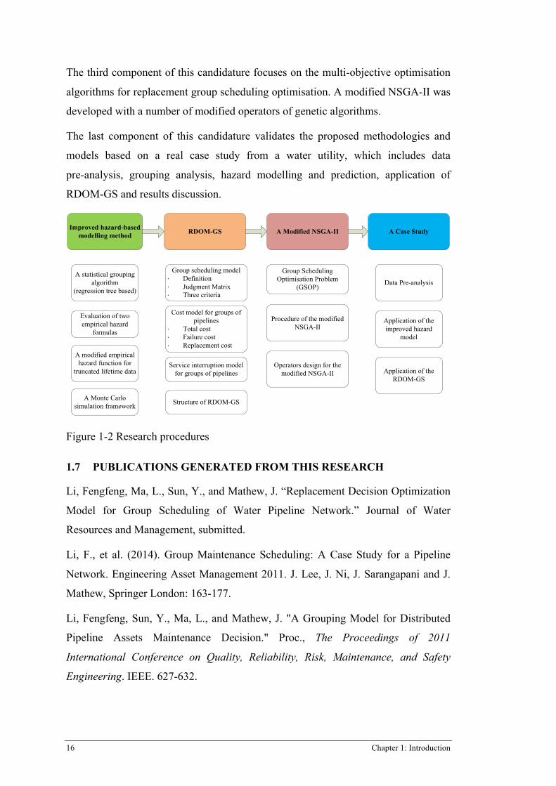
16 Chapter 1: Introduction
The third component of this candidature focuses on the multi-objective optimisation
algorithms for replacement group scheduling optimisation. A modified NSGA-II was
developed with a number of modified operators of genetic algorithms.
The last component of this candidature validates the proposed methodologies and
models based on a real case study from a water utility, which includes data
pre-analysis, grouping analysis, hazard modelling and prediction, application of
RDOM-GS and results discussion.
Figure 1-2 Research procedures
1.7 PUBLICATIONS GENERATED FROM THIS RESEARCH
Li, Fengfeng, Ma, L., Sun, Y., and Mathew, J. “Replacement Decision Optimization
Model for Group Scheduling of Water Pipeline Network.” Journal of Water
Resources and Management, submitted.
Li, F., et al. (2014). Group Maintenance Scheduling: A Case Study for a Pipeline
Network. Engineering Asset Management 2011. J. Lee, J. Ni, J. Sarangapani and J.
Mathew, Springer London: 163-177.
Li, Fengfeng, Sun, Y., Ma, L., and Mathew, J. "A Grouping Model for Distributed
Pipeline Assets Maintenance Decision." Proc., The Proceedings of 2011
International Conference on Quality, Reliability, Risk, Maintenance, and Safety
Engineering. IEEE. 627-632.
Improved hazard-based modelling method
Group scheduling model·∙ Definition·∙ Judgment Matrix·∙ Three criteria
RDOM-GS A Modified NSGA-II
Cost model for groups of pipelines
·∙ Total cost·∙ Failure cost·∙ Replacement cost
Service interruption model for groups of pipelines
A statistical grouping algorithm
(regression tree based)
Evaluation of two empirical hazard
formulas
A modified empirical hazard function for
truncated lifetime data
Group Scheduling Optimisation Problem
(GSOP)
Procedure of the modified NSGA-II
A Case Study
Data Pre-analysis
Application of the improved hazard
model
Application of the RDOM-GS
A Monte Carlo simulation framework Structure of RDOM-GS
Operators design for the modified NSGA-II
Chapter 1:Introduction 17
Xie, G., Fengfeng Li, et al. Hazard Function, Failure Rate, and A Rule of Thumb for
Calculating Empirical Hazard Function of Continuous-time Failure Data. The 7th
World Congress on Engineering Asset Management (2012). Daejeon, Korea.
1.8 SOME IMPORTANT DEFINITIONS
Throughout this thesis, definitions of terms are given when they are introduced.
However, definitions of some of the more important terms used in the reliability
evaluation of engineering systems and maintenance decision support are collected in
this section for easy access and reference.
As bad as old: if the condition of a repairable system after a repair is the same as it
was just before the repair, the system is said to be in an “as bad as old” condition
after the repair.
Corrective maintenance: in water network management, a strategy is corrective if
action is taken after a failure has occurred.
Covariate: all those factors that have an influence on the reliability characteristics of
a system are called covariates. Covariates are also called variables, explanatory
variables or risk factors. Examples of covariates include environmental factors (e.g.
soil condition), hydraulic factors (e.g. pressure) and structural variables (e.g.
diameter)
As good as new: If the condition of a repairable system after a replacement is reset to
that of a new system, the system is said to be in an “as good as new” condition after
the replacement.
Data grouping: Failure records may contain distinctive distribution features in
different groups, which can be identified with properly grouped pipes in terms of
pipe length, diameter, material types, installation year and soil types. Data grouping
is to partition pipes’ data into more homogeneous groups, where the hazard curves
between groups are clearly distinctive from each other.
Group scheduling: Given a water pipes’ network of N individual pipes with an
inventory of their information, given a replacement-planning period of T years, how
the pipes or pipe segments should be scheduled into groups of replacement activities
is based on multiple criteria to meet multiple objectives.
Hazard/hazard rate: Instantaneous failure rate.
18 Chapter 1: Introduction
Lifetime: The concept of lifetime applies only for components, which are discarded
the first time they fail. The lifetime of a component is the time from when the
component is put into function until the component fails.
Pipe: pipe is identified from one node in the water network to another (e.g. manhole,
network junction). Each pipe normally consists of a number of “pipe segments”.
Pipe segment: the smallest unit of pipe, which is linked one-by-one through welding
process or flange. The pipe segment is determined by the standard construction of
pipe.
Pipeline: pipeline contains a number of pipes connected with joints and valves. It is a
general statement of a number of water pipes. Pipeline replacement means
replacement activities conducted at a number of specific pipes.
Proactive maintenance: In water network management, a strategy is proactive if a
maintenance action is taken before a failure occurs.
Rehabilitation: All methods for restoring or upgrading the performance of an existing
pipeline system. The term rehabilitation includes repair, renovation, renewal and
replacement.
Renewal: Construction of a new pipe, which fulfils the same function in the
distribution system but does not necessarily have an identical path to the pipe it is
replacing.
Renewal process: A failure process for which the times between successive failures
are independent and identically distributed with an arbitrary distribution. When a
component fails, it is replaced by a new component of the same type, or restored to
“as good as new” condition. When this component fails, it is again replaced, and so
on.
Renovation: Methods of rehabilitation in which all or part of the original fabric of a
pipeline are incorporated and its current performance improved. Relining is a typical
example of pipe renovation.
Repair: An unplanned maintenance activity carried out after the occurrence of a
failure. After the repair, the system is restored to a state in which it can perform a
required function (e.g. supplying water). (Rectification of local damage)
Chapter 1:Introduction 19
Replacement: Construction of a new pipe, on or off the line of an existing pipe. The
function of the pipe will incorporate that of the old, but may also include
improvements.
Water pipe failure: break or leakage on a pipe.
Water main: a principal supply pipe in an arrangement of pipes for distributing water
in water pipe network.
1.9 THESIS OUTLINE
The thesis is primarily composed of seven chapters.
Chapter 1 Introduction
The topic and the scope of the research program are presented. The objectives of the
research program and the methods used to achieve the research objectives are
described. The outcomes of the research and the innovative contributions made by
the candidate are identified.
The rest of this thesis is organised as follows:
Chapter 2 Literature Review
The literature review of this thesis consists of four parts corresponding to the
identified research objectives. The first part reviews the significance of the water
pipe failures followed by the discussion of the causes of failures of water pipelines.
The second part focuses on statistical modelling for pipeline failures. The limitations
and advantages of these models are discussed and summarised as well. The third part
reviews the decision support method and models for water pipeline replacement
optimisation, followed by the methodologies of multi-objective optimisation at the
end of this chapter.
Chapter 3 Am Improved Hazard-based Modelling Method for Water Pipelines
In this chapter, an improved hazard-based modelling method for reliability analysis
of water pipelines is developed. An introduction of linear assets is discussed,
followed by an introduction of the piecewise hazard model for linear assets.
Moreover, a statistical grouping algorithm, which partitions all water pipes into
relatively more homogeneous groups, is developed, followed by a comparison study
of two empirical hazard formulas. Furthermore, an empirical hazard model to deal
20 Chapter 1: Introduction
with truncated lifetime data and a hazard distribution fitting method is developed,
followed by a validation based on test-bed sample data sets generated by Monte
Carlo simulation. The procedure of the improved hazard model for linear assets is
summarised at the end of this chapter.
Chapter 4 A Replacement Decision Optimisation Model for Group Scheduling
This chapter proposes a multi-objective replacement decision optimisation model for
group scheduling (RDOM-GS), which starts at the maintenance decision support on
water pipe with the economics of repair and replacement. Then, cost functions for
water pipe repair and replacement were introduced and developed, based on the
improved hazard model developed in Chapter 3. Group replacement scheduling was
discussed, and a judgment matrix and three integrated models for replacement group
scheduling were developed. A new replacement cost function for group scheduling
was developed, followed by the model for dealing with the customer service
interruption. The objectives and constrains for RDOM-GS was summarized,
followed by an introduction of the structure of the RDOM-GS.
Chapter 5 An Improved Multi-objective Optimisation Algorithm for Group
Scheduling
This chapter proposes an improved multi-objective optimisation algorithm for
replacement group scheduling optimistion problem (GSOP). It starts with a
mathematical description of the GSOP followed by the analysis of its computational
complexity. A modified NSGA-II to deal with GSOP was introduced, which includes
a procedure and the operators. A comparison study for the modified NSGA-II and
original NSGA-II based on two simplified objective functions was conducted at the
end of this chapter.
Chapter 6 Case Study from a Water Utility
In this chapter, a case study was conducted using the data collected from a water
utility to validate the proposed models. The chapter begins with a data pre-analysis,
then a grouping analysis, hazard prediction, application of RDOM-GS and finally,
results comparison.
Chapter 7 Conclusions and Future Works

Chapter 1:Introduction 21
The last chapter concludes the thesis and summarises the contributions and work of
this candidature. Some possible research directions are also identified. These
research directions can be pursued in the future as an extension of this candidature.
Throughout this study, a mathematic software tool MATLAB is used in most of the
statistical analysis, and optimisation analysis. The software package Microsoft
Access 2007 is used for raw data processing.

Chapter 2: Literature Review 23
Chapter 2: Literature Review
This chapter includes the review of literature on water pipe failures; statistical
modelling methods for reliability analysis of pipe failures; methods and models of
maintenance decision-making for water pipes; multi-objective optimisation methods.
The research gaps are discussed in the last section.
2.1 WATER PIPE FAILURES
2.1.1 Consequences of water pipe failures
Water pipe is a type of infrastructure asset. When the pipe fails, the consequences
may include loss of water, urgent and unscheduled maintenance activities,
interruption of service, system performance decrease, consumer dissatisfaction,
property damage, inefficient use of funds, and even catastrophic consequences. Some
of these consequences tend to be either interrelated, or interact with each other,
leading to more expensive scenarios. For example, loss of water service to
commercial sites, which depend largely on water for servicing their customers,
would lead to business loss. In some cases, undetected failed water pipes may create
sinkholes by washing away the bedding underneath roads, which poses a hazard to
both vehicular and pedestrian traffic.
With the aging of the water pipes, failures have been occurring with increasing
frequency in recent years. According to a record [1], approximately 850 water main
breaks have occurred in North America each day. Since January 2000, 4,019,274
broken water mains in North America have been recorded, and the costs are
estimated around $US 40 billion, not including the high costs of emergency
equipment, depleted water supply, traffic disruptions, and lost work time. Some of
the water pipe failures can lead to severe disasters such as causing the interruption of
water services, blocking road, and polluting the environment.
The situation for Australia is far from optimistic. Between 2009 and 2010, Adelaide
recorded 22.4 failures per 100 km of pipe length, compared with 28.4 in Sydney, 37
in Brisbane and as much as 50 in Melbourne, according to the records from the

24 Chapter 2: Literature Review
Water Services Association of Australia (WSAA)[17]. Some real examples of water
pipe failures in Australia from the middle of 2010 to 2012 can be found in literature.
A water pipe ruptured in Brisbane's CBD on June 17th, 2010, leaving a large tear in
the road and sending water gushing past alarmed pedestrians [18]. Two burst water
mains led to a water shortage in Brisbane's north eastern suburbs on September 10th,
2011, and bottled water had to be supplied to the public for those suburbs [19]. A
water main in Adelaide burst, flooding one car park on January 2nd, 2012, spilling
into side streets and along footpaths [20]. Traffic in the morning peak was disrupted
by a burst water main in central Adelaide on May 17th, 2012, which left a deep hole
in the road [21]. Water cascaded down a street in Sydney on July 3rd, 2012, when a
water pipe burst, flooding up to 12 houses and causing a burst of a gas main, with a
road and a driveway upended and torn apart [22]. A number of months later, on
October 29th, 2012, a water main burst in Glen Waverley, in Melbourne's eastern
suburbs; up to 2 million litres of water were lost in the rupture as water shot up to 50
metres into the air for about an hour in the residential suburb. More than 100,000
homes were affected by the rupturing. A house suffered water damage, and a metal
cage covering the main's pressure release valve was blown off and landed about 15
metres away, damaging the roof of a carport. The burst pipe was about 50 years old
and had no history of failure [23].
2.1.2 Failure modes of water pipe
Water pipe failure is a general description of the water pipe’s state of not functioning,
which includes a number of modes. WSAA [24] summarised the most common types
of failure modes in water supply mains, which includes pieces blown out, perforation,
broken back (circumferential break), longitudinal split, pipe wall rupture/tear
associated with or during tapping, leaking joints, and third-party damage.
A number of factors influence the degradation of water pipes. The causes of water
pipe failures can be classified into two major categories based on the physical
degradation of water pipes, internal and external reasons. The factors, which were
commonly assumed to have the greatest impact on pipe failure, include pipe’s age,
installation period, corrosion, diameter, length, material, seasonal variation, soil
condition, pressure, nearby excavation. [25].

Chapter 2: Literature Review 25
A pipe’s structural variables, such as material, length and diameter, play a significant
role on water pipe failure analysis. For example, according to a pipe’s structural
ability, all materials can be classified with two categories, rigid material and flexible
material. The rigid material pipes sustain applied loads by means of resistance
against longitudinal and circumferential bending, while the flexible material pipes
are pipes that deflect more than 2% of their diameter without any sign of structural
failure. The categories of material for water pipes according to their structural ability
are given in Table 2-1.
Table 2-1 Categories of water pipe material and abbreviations
Categories Class Material Abbr.
Rigid Concrete & Cement
Concrete CONC Reinforced Concrete Pipe RCP Steel Concrete Lined SCL Mild Steel Concrete Lined MSCL Asbestos Cement AC Vitrified Clay VC Fibre Reinforced Cement FRC Cast Iron Cement Lined CICL Ductile Iron Cement Lined DICL
Metal
Cast Iron CI
Flexible
Assumed Copper ECOP Copper CU Galvanized Wrought Iron GWI Steel STEEL Galvanised Steel GAL Mild Steel MSCL
Plastic
Glass Reinforced Plastic GRP Poly Vinyl Chloride PVC Modified PVC MPVC Unplasticised Poly Vinyl Chloride UPVC Polyethylene PE High-Density Polyethylene HDPE Medium Density Polyethylene MDPE Fibre Reinforced polyester Pipe FRP
Various types of material show different structural ability that lead to the differences
of other factors that predominantly are the influence of pipe failures. For example,
climate and clay soil conditions were the two critical factors for AC pipe failure [26],
while the failure of UPVC pipes were more attributed to poor installation, excessive

26 Chapter 2: Literature Review
operating conditions, third-party damage or poorly manufactured solvent cement
joints [27].
2.1.3 Replacement cost on water pipes
Due to the increasing trends of degradation and failures, maintenance of water pipes
have become the major concerns of water utilities, particularly in the developed
countries where a large number of water pipes have been established with a huge
amount of previous investments.
Millette and Mavinic [28] indicated that Toronto city budgeted $US5 million in
water distribution system repair due to corrosion in 1983, and the city of Winnipeg
spent $US7.7 million for the same purpose. In the United States, the annual corrosion
costs for maintenance of water pipelines are up to $US700 million, without the
consideration of costs incurred for the repair of private water systems [28]. In Alaska,
Alyeska maintained and operated the Trans-Alaskan Pipeline in 800 miles of pipeline
from Alaska’s North Slope oil fields to the port at Valdez. The project cost $US72
million [29]. Sydney Water awarded its Asia Pacific operation two contracts for
small and medium diameter sewer and storm water pipeline rehabilitation. The
combined three-year term contracts were lnsituform’s largest award in Australia to
date and had a budgeted value of $US27 million, with the potential for additional
work [30]. The city of Durban in South Africa invested $US205 million to replace
1,750 km of ageing water pipe with trenchless technology. The new pipes have a
fifty year lifespan and should significantly reduce the number of bursts, saving the
municipality $US31.8 million per year [31]. In 2011, the Environmental Protection
Agency of USA (EPA) invested $388,000 in the City of Russell, Kansas for
improving its drinking water system. The purpose of the project was to replace old,
deteriorating cast iron pipes with new plastic piping [32].
According to a record from the American Water Works Association (AWWA), more
than one million miles of pipes are nearing the end of their useful life and
approaching the age at which they need to be replaced [2], and these replacement
costs combined with projected expansion costs will cost more than $US 1 trillion
over the next two of decades [3].
All the investment schemes mentioned above have the objectives of improving
drinking water systems and preventing water pipe failures thereby replacing old

Chapter 2: Literature Review 27
pipes with new ones. This leads to two research issues, (1) water pipe failure
prediction based on statistical modelling, and (2) maintenance decision making for
water pipes concerning how the replacement activities should be planned and
scheduled taking into account multiple concerns.
2.2 RELIABILITY ANALYSIS FOR WATER PIPE NETWORKS
Reliability analysis plays a significant role in improving the performance of water
pipe networks. System reliability is the probability that the system will perform its
intended function for a specified interval of time under stated conditions [33].
A comprehensive review of the statistical models for structural deterioration of water
mains before 2001 was conducted by Kleiner and Rajani[34]. They attempted to
quantify the structural deterioration of water mains by analysing historical
performance data. They classified the statistical methods into deterministic and
probabilistic models. Their review provided descriptions of the various models
including their governing equations, as well as critiques, comparisons and
identification of the types of data that are required for implementation. Over recent
years, a number of efforts were made to get better prediction results for water pipe
failures.
A comparison study [35] for the log-linear ROCOF and the power law process using
the maximized log-likelihoods was conducted to model the failure rate of the
individual pipes. The study found that the log-linear ROCOF showed better
performance than the power law process, when the ‘failure-time-based’ method was
used. Recording each failure time resulted in better modelling of the failure rate than
observing failure numbers in some time intervals. Wang and Zayed [36] developed a
deterioration model which was applied to predict the annual break rates of water
mains considering pipe material, diameter, age, and length based on five multiple
regression models. This model analysed the deterioration trends of water mains, and
it had limitations in interpreting the conditions of water mains. Fahmy and
Moselhi[37] presented a failure forecasting model based on artificial neural
networks (ANNs) to predict the remaining useful life of cast iron water mains, which
was used to determine condition rating of the water mains. The model takes into
account factors related to pipe properties, its operating conditions, and the external
environment that surrounds the pipe. An ANNs based failure estimation model [38]
28 Chapter 2: Literature Review
was developed to predict the water mains failure and the determination of the benefit
index for a city in the north of France. Six ANNs models were established on the
basis of preliminary database analysis, which were constructed using a
cross-validation approach. A framework of dynamic deterioration models[39] was
developed combining individual prediction and group prediction. This model can
avoid the uniform treatment of the entire sewer pipe network using the clustering and
filtering process on the basis of location-related attributes and operational conditions.
I-WARP [40] was developed based upon an non-homogeneous Poisson process
(NHPP) to model breakage rates in individual water mains, which considered both
static (e.g., pipe material, pipe size, age (vintage), soil type) and dynamic (e.g.,
climate, cathodic protection, pressure zone changes) factors.
When analysing the reliability of water pipes, existing models often consider the
entirety of pipes in the pipe system. However, water pipes are typical linear assets;
they do not have a clear physical boundary and usually span long distances, which
can be divided into segments[41]. Each segment performs the same function but may
be subject to different loads and environmental conditions. The failure of one pipe
segment may not affect the reliability of other segments. Therefore, a water pipe
should be treated as a number of segments. However, most of the existing models
fail to consider the individual contributions of different segments of the pipe to the
reliability of the system.
To deal with the segmentation issue in reliability analysis of water pipes, Sun et al.
[13] proposed a piece-wise hazard model for linear assets. This model often
experiences difficulty in analysing real lifetime data for water pipes. Failure records
may contain distinctive distribution features in different groups, which can be
identified through pipe length, size, material types, installation year, soil types,
season. A fundamental issue for applying this model is the data grouping for
reliability analysis [13]. Data grouping that aims to sub-divide the observation space
into characteristically more homogeneous subgroups is necessary before reliability
analysis.
Two questions need to be answered: what criteria should be used to form groups, and
how many groups should be partitioned? The number of partitioned groups should
balance two aspects: (1) homogeneity in each subgroup, and (2) enough failure data
for hazard calculation. The more groups partitioned, the more homogeneous the

Chapter 2: Literature Review 29
characteristics within each group are, but fewer are the observations left in each
subgroup for statistical analysis.
The literature provides a number of approaches to partition water pipe data into
groups based on specific characteristics. Some categorize pipes based on engineering
expert knowledge [42]. This type of approach has an advantage, in that grouping is
based on practical experience for pipe characteristics and its failure modes. For
instance, different materials have different physical characteristics, which may lead
to different failure modes and failure rates. However, these methods only take
materials and ages into consideration. An approach based on the one and two-way
analysis of variance (ANOVA) has been developed [43] to analyse failure data. It
groups data on breaks and establishes breakage rate patterns for each group.
However, grouping criteria needs to be decided, first based on prior knowledge,
before ANOVA to validate the grouping results. In general, prior knowledge of
grouping criteria needs to be investigated. Moreover, it is assumed that the breakage
rate is followed by an exponential increase over time, which in some cases is not in
accord with the facts.
Therefore, a data grouping method needs to be developed, which can be used to
analyse water pipe data, partition pipes into homogeneous groups, and
simultaneously, keep sufficient sample size of failure data. Further literature review,
specific to empirical hazard functions in reliability prediction models, is presented in
the following chapters.
2.3 MAINTENANCE DECISION MAKING FOR WATER PIPE NETWORK
2.3.1 Maintenance strategy
Maintenance is considered as a key activity for water utilities to prevent water pipe
failures and enhance network performance. It contributes to service with quality, and
enriches all the company experience surrounding the service provided. In this section,
the candidate has found references to three different types of maintenance strategies
applied in distributed infrastructure network companies, including corrective
maintenance, preventive maintenance, and predictive maintenance, which are
described below:

30 Chapter 2: Literature Review
Corrective maintenance (CM) can be defined as the maintenance that is required
when an item has failed or worn out, to bring it back to working order. Corrective
maintenance is carried out on all items where the consequences of failure or wearing
out are not significant and the cost of this maintenance is not greater than
preventative maintenance [44]. In current practice, maintenance providers often do
corrective maintenance to a small range of pipe (some pipe segments, rather than all
segments of the pipe) near a leak or rupture. This activity may consist of repair or
restoration of pipes, and will be the result of a regular inspection, which identifies the
failure in time for corrective maintenance.
Preventative maintenance (PM) is maintenance that is carried out to prevent an item
failing or wearing out by providing systematic inspection, detection and prevention
of incipient failure. Predictive Maintenance is often applied to aged pipelines to
reduce unexpected failures and their resultant undesirable impacts. To improve the
network reliability and prevent the failure from happening, maintenance people
replaced particular old pipes with all new ones. Two commonly used PM policies
include time based preventive maintenance (TBPM) and reliability based preventive
maintenance (RBPM). In the TBPM policy, a pipeline is maintained based on
scheduled PM times. The intervals between two PM actions may or may not be the
same, whereas in the RBPM policy, a control limit of reliability is defined in advance.
Whenever the reliability of a pipeline falls into this predefined control limit, the
pipeline is preventively maintained. The purpose of PM is to improve the overall
reliability of the entire pipeline[45]. Most maintenance of water pipe planning can be
classified in RBPM.
In the predictive maintenance (PdM) technique, which is also referred to as a
condition-based PM, the maintenance schedule and frequency match the age or
health of the system at all times, making the schedule nearly optimum, prolonging
the time to replacement (TTR) as a consequence. The expected times to future failure
of a system are estimated during each operational period based on the variation
pattern of its physical properties (condition monitoring) that are indicative of its state
of degradation using implanted sensors, and the downtime schedule for each
operation cycle is determined based on the estimated future failure times[46, 47]. For
water pipes, condition assessment methods are essential for effective maintenance. A
number of direct and indirect sensing techniques/technologies for inspection and

Chapter 2: Literature Review 31
detection of water pipe failures were developed in recent years, for example, CCTV,
laser scan, electromagnetic methods, acoustic method, ultrasound methods. However,
condition assessment for a water pipe system is costly: pipes tend to be hidden
underground; they’re hard to access; they’re of different construction methods and
specifications; they can cross jurisdictional borders; and they can be distributed in
large geographical areas. In South-East Queensland, for example, one utility
company is responsible for 8,744km of pipelines scattered in a geographical territory
of 14,364 km². Therefore, the current relatively high cost of condition assessment
technologies justifies their use mainly on large water transmission pipelines, where
consequences of failure are relatively high. [48] The applications of assessment
technologies were rarely used for the water supply industry, especially for some
small water utilities.
2.3.2 Replacement decision making for water pipe network
Literature has shown numerous efforts in replacement decision making for water
pipe network. Shamir and Howard[49] made the first attempt at determining the
optimal time for water pipe replacement. Their model includes breakage rate data for
each pipe and the present value costs of replacement and maintenance. It was a
highly simplified approach, and many important elements were omitted in
rehabilitation planning. Optimization techniques were regarded as the interaction of
each water pipe with the network system as a whole. They considered both the
performance and cost of the replaced system in the formulation of the replacement
and renewal program. Based on that, a number of approaches had been reported,
which contain the optimization of performance given a cost constraint [50] and the
minimization of cost given a performance constraint[51, 52]. These optimization
techniques were used to be applied in network replacement as a multi-objective
problem [53]. The optimization technique allowed for the trade-off between cost of
replacement and system performance. However, such techniques require large
numbers of trial evaluations to obtain near-global optimal solutions. System
availability as a performance measurement based on the Markov model was
developed[50]. They modelled the states of deterioration of a pipeline and included
the state of planned rehabilitation. Therefore, the decision about whether to replace
or repair could be made to maximize the probability that the pipeline was operational
at any time in its deterioration. Lansey, Basnet, and Woodburn [54] minimized

32 Chapter 2: Literature Review
rehabilitation cost based on a hydraulic performance constraint. They considered
two-time steps such that works were scheduled for the current time and in 10 years.
A similar approach restricted to a single time step was used by De Schaetzen,
Randall-Smith, Savic, and Walters [55]. Engelhardt [53] extended this method by
allowing the replacements to be scheduled over a 20 year period, which was split into
four five-year time periods. The model enabled water pipelines replacements to be
scheduled in any of these time intervals, with the expenditure in each period
constrained by the available funds. This ability to schedule replacements over an
extended period allowed for the various time-dependent parameters, for example,
demand increases, to be included as part of the model.
A model was developed by Deb [56], which can extended planning horizon to
identify the time to the next rehabilitation. A cycle time between replacements for
each main in the network was proposed [56]. The model made the assumption that
water pipelines currently in service were unlined metallic, whereas the water mains
they would be replaced with would be either lined or non-metallic. The time to first
replacement was thus a function of structural deterioration through corrosion and
increase in hydraulic roughness. The duration between future replacements was
purely a function of structural deterioration. Structural deterioration was considered
as part of an economic analysis of future maintenance costs[57] in order to provide
an optimum time of replacement. The deterioration in the hydraulic efficiency of the
original water mains was modelled using the empirical hydraulic roughness model
[58]. This model was in conjunction with the hydraulic solver EPANET to ensure
that the pressures in the system remained above the minimum required, which
attempted to extend the useful economic service life of the existing main by
considering lining as opposed to replacement.
In a multi-objective approach, Halhal, Walters, Ouzar, and Savic [59] used the
rehabilitation cost as a minimization objective and the maximization of the benefits
of the rehabilitation schedule as a further objective. These benefits included the
improvement in hydraulic performance of the rehabilitated system, its increased
flexibility provided by including parallel mains, the economic savings of replacing
mains that would experience bursts, and the water quality benefits associated with
replacing old water mains. Except for savings associated with reduced numbers of
bursts, the estimation of these benefits was very subjective. Farmani, Savic, and

Chapter 2: Literature Review 33
Walters [60] reported a multi-objective approach. The first objective considered was
the minimization of operating cost. A second objective was maximizing reliability,
which was represented by a surrogate measure based on the number of customer
interruptions. Raziyeh, Godfrey, and Dragan [61] investigated the application of
multi-objective evolutionary algorithms to the identification of the payoff
characteristic between total cost and reliability of a water distribution system. It
reduced costs by reducing the diameter of some pipes, thus leaving the system with
insufficient capacity to respond to pipe breaks or demands that exceed design values
without violating required performance levels. Alvisi and Franchini [62] based on a
multi-objective genetic algorithm proposed a near-optimal rehabilitation scheduling
model, with reference to a fixed time horizon. The objectives were to minimize the
overall costs of repairing and/or replacing pipes, and to maximize the hydraulic
performances of the water network, whose constraints were represented by the
maximum costs that were allowed yearly. A head-driven hydraulic simulator was
linked to the optimizer to represent the different hydraulic and breakage scenarios,
which became possible in consequence of the rehabilitation schedules generated by
the genetic algorithm.
A multi-objective optimization algorithm NSGA-II, coupled with water distribution
network simulation software EPANET, was proposed by Atiquzzaman, Shie-Yui,
and Xinying [63] to provide Pareto front of the cost and nodal pressure deficit.
However, this method was not proved in a large water network. Dandy and
Engelhardt [6] used genetic algorithms to generate trade-off curves between cost and
reliability for pipe replacement decisions. These can identify the trade-offs necessary
for the current conditions and allowed the water authority to determine the required
levels of future expenditure, given funding constraints, to meet a specified level of
service over the entire planning horizon. A robust decision support tool for water
system rehabilitation incorporated forecast pipe failures and a strategy to solve a
multi-objective optimization problem trading investment and benefits was proposed
by Giustolisi, Laucelli, and Savic Dragan[64]. They used a burst modelling approach,
based on an evolutionary polynomial regression technique for predicting pipe bursts,
which is used in a short-term planning. The result of this model can process which
pipes were prioritized for rehabilitation based on the number of times, by considering
costs and the priority rating of each main. Werey, Llerena, and Nafi [65] proposed a

34 Chapter 2: Literature Review
decision support model that ensures the scheduling of pipe renewal according to
available financial resources based on forecasting pipe failures and evaluating future
maintenance costs. They measured the undelivered water quantity and the number of
unsupplied nodes when a considered pipe was unavailable during the peak demand
period. Based on the results, by applying this model, the reliability of a water
distribution network was enhanced. Zarghami, Abrishamchi, and Ardakanian [66]
investigated integration of leakage detection on the water distribution network, water
metering and on low volume water, and provided a model which derived optimum
long-term plans for implementation of water resources. Di Pierro, Khu, Savic, and
Berardi [67] proposed a model using multi-objective, hybrid algorithms, ParEGO
and NSGA on the design problem of a real medium-size network in Southern Italy,
and their results suggested that the use of both algorithms, in particular NSGA, could
be successfully extended to the efficient design of large-scale water distribution
networks. Nafi and Kleiner [68] focused on low-level scheduling of individual water
mains, and proposed a model for the scheduling of individual water mains for
replacement in a short-to-medium predefined planning period, subject to various
budgetary constraints. A multi-objective genetic algorithm scheme was used as a tool
to search a vast combinatorial solution space, comprising various combinations of
pipe replacement schedules.
Researchers have provided various decision support tools to assist utility managers.
Engelhardt et al. [69] and Rajani and Kleiner [70] provided comprehensive reviews
on the approaches and methods that had been developed before 2001. Since then,
some new tools have also been proposed. Sægrov [71] presented a decision support
system CARE-W to allow selection and schedule of the rehabilitation jobs taking
into account of deterioration. The system provides a hydraulic model for assessing
the reliability of a pipeline network. Jarrett et al. [72] and Moglia et al. [11]
developed PARMS-PLANNING and PARMS-PRIORITY based on risk calculation.
These two models provide assistance in optimal replacement schedules for individual
pipelines, including failure prediction, cost assessment, data exploration and scenario
evaluation. Dandy and Engelhardt [6] developed a multi-objective genetic
algorithm-based approach to finding out trade-off points between economic cost and
reliability for scheduling replacement activities. Halfawy et al. [73] developed an
integrated sewer renewal planning decision support system for estimating remaining

Chapter 2: Literature Review 35
service life and the probability of failure, and also for guiding inspection and renewal
planning decisions. Sun et al [74] proposed a new approach for predicting the
reliability of pipelines with multiple preventive maintenance cycles.
For practicality, when undertaking replacement planning, utility managers usually
select two or three pipes, organised into one group for replacement, in order to meet
some multiple objectives, i.e. minimization of costs, risks, and service interruptions,
or maximizing reliability, and work efficiency. However, this practice fails to
provide an optimal solution because of ambiguous criteria. Optimal group schedules
need to take into consideration the multiple criteria such as costs, impact of service
interruptions, pipe specifications, the type of technology employed and geographical
information.
Some researchers have worked on scheduling grouping optimizations, although
general group scheduling in replacement planning for water pipeline network has so
far not received enough attention. Kleiner et al. [75] developed a renewal scheduling
model for water main renewal planning, which takes account of life cycle costs and
contiguity savings due to reduced mobilization costs by setting a contiguity discount.
However, the model only considers two pre-determined situations where two
pipelines share the same node and both are replaced in the same year. These
pre-determined situations are not in accord with reality, because, in practice,
pipelines, which are located in the same area, might be grouped together, even when
they are not planned for replacement in the same year. Therefore, group scheduling
for water pipe replacement decision optimisation is still an open research area, which
may lead to bottom-line benefits for both utilities and customers to minimize total
cost and limiting service interruption.
2.4 EVOLUTIONARY ALGORITHMS FOR MULTI-OBJECTIVE OPTIMIZATION
Multi-objective problems are problems with two or more objectives, and these
objectives usually conflict. The main difference between multi-objective and
single-objective optimization is that a multi-objective problem does not have one
single optimal solution, but instead has a set of optimal solutions, where each
represents a trade-off between objectives. [76]
36 Chapter 2: Literature Review
One way to perform multi-objective optimization is using an evolutionary algorithm
(EA). Evolutionary algorithms are optimizers inspired by natural evolution, and with
the concept of survival of the fittest. In an EA, solutions to a given problem are
considered individuals of a population, where the fitness of individuals is attributed
by how well they solve the problem at hand. In the population, individuals may
produce offspring, which makes parents and offspring compete for inclusion in the
next generation. As only the most fit will survive, the full population improved
iteratively in each passing generation.
Multi-objective evolutionary algorithm techniques can be traced back to 1985;
Schaffer [77] presented an extension of the genetic algorithm method (vector
evaluated genetic algorithm) in which the population in each generation is divided
into sub-populations, with each sub-population being assigned a fitness on the basis
of a different objective function. Then, through the development of multi-objective
evolutionary algorithm, most of recent research can be identified as Pareto-based
approaches.
Literature has shown a great number of contributions in this area. Multi-objective
genetic algorithm (MOGA) begins with a ranking of the solutions based on the
number of solutions that dominate it, and not all possible ranks will be represented in
the population. The solutions are then sorted according to their raw fitness values
(from rank 1 to largest rank found) and a linear function is used to assign an average
fitness to each solution. Because of the computation methodology, the shared fitness
of a high ranked solution can become more than that from a low ranked solution,
which in effect can result in an inadequate selection pressure for better solutions. A
non-dominated sorting genetic algorithm (NSGA)[78] was developed, in that it uses
a non-dominated sorting procedure to calculate the raw fitness values as mentioned
in the MOGA. Firstly, a rank 1 is assigned to all non-dominated solutions in the
population. A dummy raw fitness value is assigned to each solution in this rank. The
dummy fitness value for the rank 2 solutions is chosen as a number less than the
minimum sharing fitness of rank 1 solutions. The process is repeated until every
member of the population has been assigned a fitness values. Niched Pareto genetic
algorithm (NPGA)[79] uses a modification of the binary tournament selection
operator to include sharing information in a decision. No particular fitness value is
assigned to a solution, and the quality of the solution is decided, entirely based on
Chapter 2: Literature Review 37
non-domination and a niche count. Distance-based Pareto genetic algorithm (DPGA)
[80] is an elitist Multi-objective evolutionary algorithm (MOEA) which maintains a
separate population, called the elite population Et, of non-dominated solutions, and
assigns fitness to the general population, Pt, members based on distance comparison
from the non-dominated ones. However, final fitness values in DPGA is dependent
on the ordering of the solutions in the population, in which case it is not clear
whether the diversity information is properly preserved or not. Strength Pareto
Evolutionary Algorithm 2 (SPEA2)[81] as a modified form of Strength Pareto
Evolutionary Algorithm (SPEA), which incorporates, in contrast to its predecessor, a
fine-grained fitness assignment strategy, a density estimation technique, and an
enhanced archive truncation method. Then SPEA2 was improved with a
neighbourhood crossover, mating selection Applying archive to allow holding of
diverse solutions in the objective space and variable space, which was named
SPEA2+[82], which has a more effective crossover mechanism and an archive
mechanism to maintain diversity of the solutions in the objective and variable spaces.
A very popular elitist genetic algorithm for multi-objective optimization was the
Non-dominated Sorting Genetic Algorithm (NSGA-II) [83]. It begins with a
non-dominated ranking of the merged parent and child population. Parent population
for the next generation, Pt+1, is created from the ranked solutions – low rank implies
high preference. However, unlike most of the algorithms, NSGA-II do not have any
parameters to tune, which has made it one of the most widely used MOEAs in
engineering optimization problems. In recent year, a number of contributions were
made to improve the NSGA-II for its efficiency. For example, a combined NSGA-II
and SPEA2 selection with the Differential Evolution (DE) scheme for solution
reproduction to create the Differential Evolution for Multi-objective Optimization
(DEMO)[84]; A crowding distance method designed by minimum spanning tree to
maintain the distribution of solutions for NSGA-II [85]; and a number of
improvements on efficient constraint handling method for NSGA-II [86-88].
The basic problem of optimal distribution system maintenance has been usually
considered as the minimization of an objective function representing the global
system costs in order to solve the optimal sizing and/or locating problems for the
distribution system. A number of research efforts for multi-objective optimization
methods in distributed infrastructure networks can be found and the review follows.

38 Chapter 2: Literature Review
Miranda [89] demonstrated a genetic algorithm approach to the optimal multistage
planning of distribution networks. He described a mathematical and algorithmic
model to solve the problems of the optimal sizing, timing and location of distribution
substation and feeder expansion using genetic algorithms. However, he did not
consider the multi-criteria methods in his research. In 1998, a new and efficient
genetic algorithm was presented for the optimal design of large power distribution
systems. It was similar to a mixed-integer nonlinear model, which takes into
consideration of non-linear variable costs and linearized costs respectively [90].
Ramirez-Rosado and Bernal-Agustin[57] created a new evolutionary algorithm
which is much faster than the classic one for finding out the best distribution network
reliability and at the same time minimizing the system expansion costs. The
algorithm determined the set of optimal non-dominated solutions, and allowed the
planner to obtain the optimal locations and sizes of the reserve feeders that achieve
the best system reliability with the lowest expansion costs, which are used in real life
power systems. In contrast to “traditional optimization approaches which typically
assess alternative planning solutions by finding the solution with the minimum total
cost”, Espie, Ault, Burt, and McDonald [91] proposed a methodology utilizing a
number of discrete evaluation criteria within a multiple criteria decision making
environment to examine and assess the trade-offs between alternative solutions. To
demonstrate the proposed methodology, a worked example was performed on a test
distribution network that forms part of an existing distribution network in one UK
distribution company area.
In 2004, a combination of AHP with genetic algorithms to capture the capability of
multi-criterion decision-making was proposed [92]. This algorithm allowed
decision-makers to give weightings for criteria using a pairwise comparison
approach, and provided more control on the determination of the optimization
solutions. In 2006, Kandil and El-Rayes [93] developed a practical and automated
system named the Multi-objective Automated Construction Resource Optimization
System (MACROS), and it incorporated multi-objective optimization module,
relational database module, middleware module and user interface module to
simultaneously minimize project cost and duration while maximizing project quality.
This system “generated optimal trade-offs among construction time, cost, and quality;
visualized the generated optimal trade-offs among these three important objectives;
Chapter 2: Literature Review 39
ranked the obtained optimal plans according to a set of planner-specified weights to
facilitate the selection of an optimal plan that considers specific project needs; and
provided seamless integration with commercially available project management
software to benefit from its practical scheduling and control features”. Carrano[94]
presented a multi-objective approach for the design of electric distribution networks
that considered the objectives of minimizing the overall costs and minimizing a
system failure index. A MOGA, using problem-specific mutation and crossover
operators and an efficient variable encoding scheme, was employed as the
optimization machinery for finding the Pareto-optimal solutions. A genetic algorithm
was used to solve the model, which evaluated the condition of elements, considered a
budget constraint, and suggested the optimal maintenance schedule over a specified
period of time. The extent of rehabilitation at a given time was considered as
dependent on the present condition and amount of deterioration[95]. In 2009,
Bernardon, Garcia, Ferreira, and Canha[96] created a new fuzzy multi-criteria
decision making algorithm for network reconfiguration problem, which focused on
power losses reduction. They chose the Bellman-Zadeh method[97, 98] for the fuzzy
resolution methodology, promoting final solutions belonging to the Pareto objective
space.
With infrastructure networks involving spatially distributed sites that have different
work conditions, activities, and quantities, Hegazy[99] presented a formulation of a
Distributed Scheduling Model (DSM), which was capable of generating schedules by
manually changing the options for construction methods, number of crews, the site
order, and the amount of interruption at various sites. Because the solution space of
Distributed Scheduling Model would be extremely large, Hegazy [100] used Genetic
Algorithms (GAs) to determine the optimum set of construction methods, for
scheduling, resource planning, and cost optimization in large construction programs
that involve multiple distributed sites. Using this distributed scheduling model, a
practical model for scheduling and cost optimization of highway construction was
presented[101]. Elhakeem [102] introduced a graphical approach (using
Nomographs), in order to provide a transparent tool for quick manpower planning
and sensitivity analysis. The Nomographs were utilized by practitioners to estimate
the manpower needed to meet a predefined deadline, under anticipated network-level
risks due to unfavourable site conditions. Subsequently, the scheduling model was

40 Chapter 2: Literature Review
applied not only to optimize the site order, construction methods and in-house crews,
but also to suggest the location and frequency of outsourcing necessary to minimize
the cost of delivery. Based on Hegazy’s research, Elbehairy [103] presented a
Multiple-element bridge management system (ME-BMS) that integrates both
project-level and network-level decisions to enable the handling of large-size bridge
networks with thousands of bridges. The life-cycle analysis also was formulated into
two sequential optimizations for the project level and the network level, respectively.
2.5 CONCLUDING REMARKS
Through this literature review, the researcher finds that multi-objective maintenance
decision optimization considering group scheduling is still an open area. In practice,
replacement activities are usually scheduled in groups manually based on expert
experience, and replacement decisions are made for groups of pipes case-by-case in
order to improve work efficiency, and to reduce costs. This practice fails to provide
an optimal solution, because the optimised replacement solutions cannot be
determined only by user experiences. Moreover, much of the existing literature [6, 8,
11, 12] only focused on analysing scheduling optimisation for individual/single pipes,
which provided replacement schedules for each single pipe to deliver an optimal
replacement year. However, these efforts cannot satisfy the practical requirements
for group scheduling optimisation in the following aspects:
(1) The requirement for integrating multiple criteria
Group scheduling needs to take into consideration multiple criteria, e.g.
minimising geographical information, maximising equipment utilisation,
minimising service interruption. Effective methods for modelling multiple group
scheduling criteria are still not available in the literature.
(2) The requirement for cost and service interruption models to deal with cost and
interruption reduction in terms of group scheduling pipes
Most of existing cost models and service interruption models for water pipe
replacement were developed for individual water pipes, which cannot be directly
applied for group scheduling, because the cost saving or interruption reduction
based on group scheduling replacement cannot be calculated. Therefore, new
costs model and service interruption models considering cost and interruption
reduction needs to be developed.
Chapter 2: Literature Review 41
(3) The requirement for optimisation algorithm to consider both replacement time
and pipe allocation
Group scheduling for water pipe replacement optimisation is complex in its large
number of decision variables, which could be in both time and space domains.
Through the literature review, it is seen that existing optimisation algorithms
used for replacement optimisation cannot be applied directly to deliver optimal
solutions. This is because they are unable to consider pipe allocation in the
algorithm, so that they can only optimise replacement for single pipes rather than
group scheduling of pipes. Therefore, a new optimisation algorithm to deal with
pipe allocation and pipe replacement year is necessary for replacement group
scheduling of water pipes.
Thus, based on the discussion above, effective methodologies for optimising of
replacement scheduling for groups of pipes are still not available.
In order to deliver optimal replacement time for groups of pipes, reliability prediction
analysis is crucial in this research. When analysing the reliability of water pipe,
existing models often consider the entirety of the water pipes rather than the
individual contributions of different components of the water pipes to the reliability
of the water pipe system. A discrete hazard modelling method [104] was developed
for general linear assets to deal with the effects caused by segmentation of pipes.
However, this model has several limitations to deal with real water pipes.
(1) It is unable to handle the multiple failure characteristics and mixed failure
distributions of water pipes
Water pipes often present multiple failure characteristics and follow mixed
failure distributions over their life spans. Failure records may contain distinctive
distribution features in different groups, which can be identified with properly
grouped pipes in terms of pipe length, diameter, material types, installation year,
and soil types. One of fundamental limitations for applying the existing hazard
model [13] is the requirement for the statistical grouping to partition assets data
based on their specific features. Existing approaches [42, 43] in the literature,
partition water pipes into groups on an ad hoc basis. Two limitations have been
identified:
a) Grouping relying on prior knowledge

42 Chapter 2: Literature Review
b) Breakage rate following an exponential increase
However, prior knowledge of grouping criteria should be one of the results of
grouping analysis, which is hardly available before any grouping analysis. The
assumption of breakage rate following an exponential increase is, sometimes, not
in accord with reality. Therefore, an effective approach for statistical grouping
had not yet been developed in reliability analysis for water pipes.
(2) It is unable to deal with complex censorship pattern of lifetime data
In practice, maintenance histories are typically available for a relatively short
and recent period, often less than a decade. The irregular, non-random
distribution of pipe installations combined with the short observation period of
failures often produce a complex censorship pattern, which is not amenable to
treatment by existing hazard models in previous research. Existing hazard
models may lead to underestimation of the true hazard for truncated lifetime data.
The methods in hazard modelling for reliability prediction analysis to deal with
truncated lifetime data have not been well developed.
(3) It is not clear about the application differences between two empirical hazard
formulas.
Through literature review, two empirical hazard formulas can be derived from
the theoretical hazard function[14-16]. One of the equations is commonly used
to calculate empirical hazard. However, previous research did not investigate
the difference of the two equations in terms of derivations and applications. This
difference may result in deviation of calculating the empirical hazard.

Chapter 3: Improved Hazard based Modelling Method 43
Chapter 3: Improved Hazard based Modelling Method
3.1 INTRODUCTION
Water pipes are typical linear assets, also called continuous assets. Linear assets are
engineering structures that typically span long distances and can be divided into
different segments. All segments perform the same function but may be subject to
different loads and environmental conditions[41]. Linear assets play an important
role in modern society, which include water pipes, sewer pipes, roads, railways, oil
and gas pipelines and electricity distribution networks.
Reliability analysis and failure prediction for linear assets have attracted a great deal
of attention from engineering asset management. However, reliability prediction of
linear assets is still a great challenge in practice. A fundamental issue is the
segmentation of linear assets and data grouping for reliability analysis. A single
linear asset may be subject to various working environments, having different failure
rates in different areas, and thus needs to be divided into distinct segments for
reliability analysis[41]. Therefore, every linear asset can be treated as a chain
structure, where the success of the whole asset depends on the success of all the
segments of this asset. In other word, if one segment fails, the relevant asset will be
treated as failed. However, the failure of one segment of the asset cannot affect the
reliability of other segments, due to its long length. A sketch to illustrate the
segmentation of water pipe is shown in Figure 3-1.

44 Chapter 3: Improved Hazard based Modelling Method
Figure 3-1 Sketch of water pipe segmentation Take water pipe as an example. A water pipe can be considered as a combination of a
number of small length segments. A segment has identical diameter, material, with
identical soil condition. One segment’s failure causes the whole pipe to lose its
functionality. From the data analysis point of view, the recorded failure history is for
water pipes rather than pipe segments. This type of record presents a gap between the
data required for reliability analysis and real failure history records.
Sun[13] proposed a discrete hazard based modelling method for linear assets. He
assumed the lifetimes of assets followed a piece-wise distribution. His method can
effectively model the hazard of linear assets based on segmentation. However, a
number of improvements are required to achieve accurate prediction results: (1)
linear assets often present multiple failure characteristics and follow mixed failure
distributions over their life spans. It is compulsory to partition water pipes into
characteristically more homogeneous groups; (2) truncated lifetime data may cause
underestimation of the true hazard.
Therefore, an improved hazard modelling method for linear assets is developed for
analysing the reliability of water pipe system. This chapter starts with an introduction
of the piece-wise hazard model developed by Sun in Section 3.2, followed by a
statistical grouping algorithm in Section3.3, which partitions all the water pipes into
characteristically more homogeneous groups. For each homogeneous group, a
theoretically sound and accurate empirical hazard function for linear assets is
necessary for analysing lifetime distribution of the continuous-time failure data, two
commonly used empirical hazard function are investigated and compared in terms of
their derivations and applications in Section3.4. In Section 3.5, an empirical hazard
Welded Joint
water pipe
Welded JointValveValve
Other pipe Other pipe
pipe segment pipe segment
under ground

Chapter 3: Improved Hazard based Modelling Method 45
function to deal with truncated lifetime data, and a hazard distribution fitting method
for an extreme situation are developed, where the extreme situation indicates large
proportion of length of pipes were repaired in the observation period. A Monte Carlo
simulation framework based on a real water utility is developed and a test-bed
sample dataset are generated based on the main features of the real data of a water
utility to test and validate the proposed empirical hazard function and the hazard
distribution fitting method in Section 3.5. Finally, Section 3.6 introduces the
procedure of the improved hazard modelling method for linear assets.
In this chapter, only water pipe is considered for the purpose of model validation
through a case study. The contribution of the proposed improved hazard modelling
method can be applied to all linear assets.
3.2 THE DISCRETE HAZARD BASED MODELLING METHOD FOR LINEAR ASSETS
3.2.1 Piece-wise hazard model for linear asset
The bathtub shape curve is a common failure rate pattern for many engineering
assets/components over their lifetimes. The bathtub hazard curve can be divided into
three parts as shown in Figure 3-2 [105].
Figure 3-2 Bathtub hazard rate curve Various models have been proposed to describe the mixed distributions[33, 106, 107].
Sun[13] proposed a piece-wise hazard model for linear assets. In his model, he
assumed that Phase I is either very short or the burn-in factors are insignificant for
II IIII
Time t
Useful life period Wearout periodBurn-inperiod
h(t)
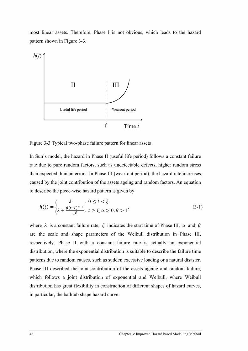
46 Chapter 3: Improved Hazard based Modelling Method
most linear assets. Therefore, Phase I is not obvious, which leads to the hazard
pattern shown in Figure 3-3.
Figure 3-3 Typical two-phase failure pattern for linear assets In Sun’s model, the hazard in Phase II (useful life period) follows a constant failure
rate due to pure random factors, such as undetectable defects, higher random stress
than expected, human errors. In Phase III (wear-out period), the hazard rate increases,
caused by the joint contribution of the assets ageing and random factors. An equation
to describe the piece-wise hazard pattern is given by:
ℎ 𝑡 =𝜆 , 0 ≤ 𝑡 < 𝜉
𝜆 + ! !!! !!!
!!, 𝑡 ≥ 𝜉,𝛼 > 0,𝛽 > 1
, (3-1)
where 𝜆 is a constant failure rate, 𝜉 indicates the start time of Phase III, 𝛼 and 𝛽
are the scale and shape parameters of the Weibull distribution in Phase III,
respectively. Phase II with a constant failure rate is actually an exponential
distribution, where the exponential distribution is suitable to describe the failure time
patterns due to random causes, such as sudden excessive loading or a natural disaster.
Phase III described the joint contribution of the assets ageing and random failure,
which follows a joint distribution of exponential and Weibull, where Weibull
distribution has great flexibility in construction of different shapes of hazard curves,
in particular, the bathtub shape hazard curve.
II III
Time t
Useful life period Wearout period
h(t)
!

Chapter 3: Improved Hazard based Modelling Method 47
The piece-wise hazard model in the wear-out period (𝑡 ≥ 𝜉) proposed by Sun[13], is
actually a simplified bi-Weibull Model [14, 108], where the hazard function is given
by:
ℎ 𝑡 = !!∙!!!!!
!!!!+ !!∙!!!!!
!!!! , (3-2)
where 𝛼! and 𝛼! are the scale parameters for two independent Weibull
distributions, and, 𝛽! and 𝛽! are the shape parameters for the two independent
Weibull distributions. The density function of the bi-Weibull model corresponds to
the smaller one of the two independent Weibull distributions. The piece-wise hazard
function can be derived from bi-Weibull distribution, where one of the shape
parameters 𝛽! or 𝛽! equals “1”. Therefore, the piece-wise model in the wear-out
period (𝑡 ≥ 𝜉) follows the joint distribution of exponential and Weibull distributions
Based on the bi-Weibull distribution, the probability density function (pdf),
cumulative distribution function (cdf) and the reliability function of the piecewise
model are given by:
𝑓 𝑡 =𝜆 ∙ 𝑒!!" , 0 < 𝑡 < 𝜉
! !!! !!!
!!∙ 𝑒!
!!!!
!
, 𝑡 ≥ 𝜉,𝛼 > 0,𝛽 > 1, (3-3)
cdf
𝐹(𝑡) =1− 𝑒!!" , 0 < 𝑡 < 𝜉
1− 𝑒!!" ∙ 𝑒!!!!!
!
, 𝑡 ≥ 𝜉,𝛼 > 0,𝛽 > 1, (3-4)
and reliability function
𝑅 𝑡 =𝑒!!" , 0 < 𝑡 < 𝜉
𝑒!!" ∙ 𝑒!!!!!
!
, 𝑡 ≥ 𝜉,𝛼 > 0,𝛽 > 1 . (3-5)
Figure 3-4 shows the nature of the functions associated with the piece-wise model for
𝜉 = 30, 𝜆 = 0.01, 𝛽 = 1.1, and 𝛼 = 50. The upper left graph indicates failure
density function; the upper right is failure distribution function; the lower left
showed reliability function; and the lower left illustrated hazard function.
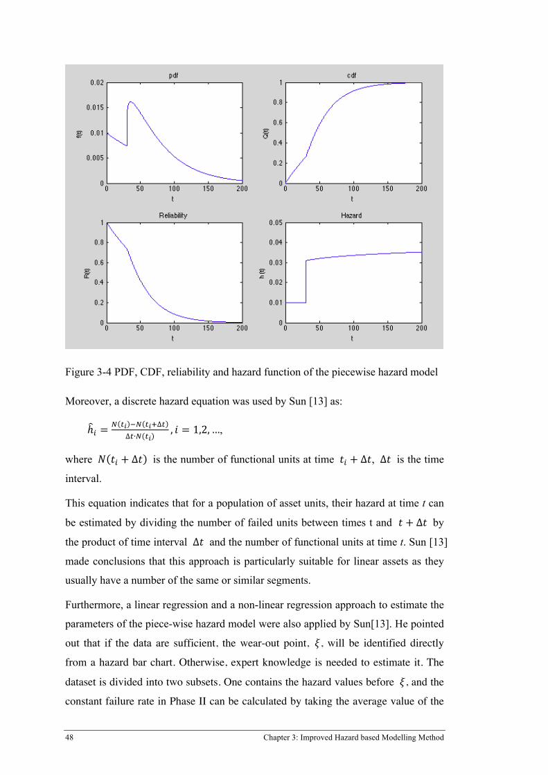
48 Chapter 3: Improved Hazard based Modelling Method
Figure 3-4 PDF, CDF, reliability and hazard function of the piecewise hazard model Moreover, a discrete hazard equation was used by Sun [13] as:
ℎ! =! !! !! !!!∆!
∆!∙! !!, 𝑖 = 1,2,…,
where 𝑁 𝑡! + ∆𝑡 is the number of functional units at time 𝑡! + ∆𝑡, ∆𝑡 is the time
interval.
This equation indicates that for a population of asset units, their hazard at time t can
be estimated by dividing the number of failed units between times t and 𝑡 + ∆𝑡 by
the product of time interval ∆𝑡 and the number of functional units at time t. Sun [13]
made conclusions that this approach is particularly suitable for linear assets as they
usually have a number of the same or similar segments.
Furthermore, a linear regression and a non-linear regression approach to estimate the
parameters of the piece-wise hazard model were also applied by Sun[13]. He pointed
out that if the data are sufficient, the wear-out point, 𝜉, will be identified directly
from a hazard bar chart. Otherwise, expert knowledge is needed to estimate it. The
dataset is divided into two subsets. One contains the hazard values before 𝜉, and the
constant failure rate in Phase II can be calculated by taking the average value of the

Chapter 3: Improved Hazard based Modelling Method 49
discrete hazard rates. The other subset contains the hazard values after 𝜉. The other
parameters of the discrete hazard model can be estimated using non-linear
regression.
3.2.2 Assumptions of the piece-wise hazard model
The failure of water pipe can lead to severe disasters such as flooding the road,
damaging the surrounding infrastructure and decreasing the pressure of water supply
so as to interrupt service to customers. The failure of one pipe segment may affect
the condition of other pipe segments adjunct to the failed segment. For example, their
conditions may be degraded by the floodwater. In practice, it is difficult to analyse
the effects because of lack of relevant information and records. To simplify the
analysis, three important assumptions were made by Sun[13] to specify the hazard
calculation for linear assets:
1. Assets are independent to each other, so that one asset’s failure cannot affect the
condition of other assets;
2. For every linear asset, segments are independent to other segments, so that one
segment’s failure cannot affect the reliability of other segments;
3. For one asset, no more than one segment fails at the same time;
The condition of the repaired segment is “as good as new”, meanwhile, the condition
of the whole asset remains “as bad as old”, for the reason that repaired segments,
normally only take small proportions of the whole assets.
3.3 STATISTICAL GROUPING ALGORITHM FOR HAZARD MODELLING
As previously mentioned, there is a practical challenge for hazard modelling of linear
assets failure/maintenance data, because linear assets often present multiple failure
characteristics and follow mixed failure distributions over their life spans. To
automatically partition pipes into more homogeneous groups, existing approaches in
the literature have the following limitations: (1) grouping criteria need to be
determined firstly based on prior knowledge, then the pre-decided groups were tested
by some methods. In general, the prior knowledge of grouping criteria is the one that
needs to be investigated. (2) They assumed the breakage rate following an
exponential increase, which in some cases is not in accord with the facts.

50 Chapter 3: Improved Hazard based Modelling Method
To deal with these limitations, and to improve the current piece-wise hazard model, a
statistical grouping algorithm is developed based on a regression tree. The reasons
for applying regression tree in this research are as follows: (1) it is a non-parametric,
so that this method does not require specification of any functional form; (2) it does
not require variables to be selected in advance, where the regression tree algorithm
will identify the most significant variables and eliminate non-significant ones; (3) its
results are invariant to monotone transformations of its explanatory variables, where
changing one or several variables to its logarithm or square root will not change the
structure of the tree; (4) it can easily handle outliers, and it will isolate the outliers in
a separate node, which is very significant, because pipe data very often have outliers
due to different materials in different installation years; (5) it has no assumptions, so
that it can very easily handle the complexity of the data grouping for water pipes.
This algorithm uses recursive partitioning to assess the effect of specific variables on
pipe failures, thereby ultimately generating groups of pipes with similar distribution
features, where homogeneity of the resulting subgroups of observations can be
achieved.
3.3.1 Statistical grouping algorithm based on regression tree
Techniques of Regression Tree
Regression trees approach deals with numerical response variables Y along with a set
of explanatory variables X, where X = 𝐗𝟏,𝐗𝟐,… ,𝐗𝐮 , and u indicates the number
of explanatory variables. Regression trees represent a multi-stage decision process,
where a binary decision is made at each stage[109]. The tree includes nodes and
branches. Nodes are designated as internal or terminal nodes, where internal nodes
can be split into two children, while terminal nodes do not have any children, and
they are associated with the average value of the response variable. The regression
tree can be used to examine all independent variables X for all possible splits and
chooses the split that yields the smallest within-group variance in the two groups,
such that the two groups are homogeneous with respect to the response variable Y.
Figure 3-5 shows the structure of regression trees [110], where t with circles indicate
intermediate nodes and t with squares show the terminal nodes with predicted values
of response variable y(t).

Chapter 3: Improved Hazard based Modelling Method 51
Figure 3-5 Regression tree structure
Variables of the statistical grouping algorithm for water pipes
Grouping for water pipes is used to investigate the homogeneous groups for pipe
failures based on the explanatory variables and response variable. The variables are
discussed and determined as below:
Explanatory variables
Pipe material is one of the most important factors for pipe failure. The properties of
pipe material include impact resistance and corrosion resistance. Impact resistance is
a material’s ability to absorb an impact without damage[111]. Pipe failure might
occur if a rock fell on the pipe in a trench or if the pipe was dropped. The rigidity and
flexibility of different materials indicate how the pipe will react to impacts. Pipes
made of rigid material sustain applied loads by means of resistance against
longitudinal and circumferential bending. Rigid material includes all concrete
(MSCL, CICL and DICL), cement (AC and FRC) and cast iron pipe. Pipes made of
flexible material can deflect more than 2% of their diameter without any sign of
structural failure. Flexible material includes all metal for example steel and copper
except cast iron, and all plastic material (PVC, UPVC, HDPE and MDPE). Corrosion
t1
t2 t3
t7t4 t5 t6
t8 t9
Split 1
Split 2 Split 3
Split 4y(t4) y(t5) y(t6)
y(t8) y(t9)

52 Chapter 3: Improved Hazard based Modelling Method
resistance is another material’s ability to resistant water pipe failure. Some materials
are more intrinsically resistant to corrosion than others. Metal pipe corrosion is a
continuous process of ion release from the pipe into the water, while plastic and
concrete pipes tend to be resistant to corrosion. Due to the differences among the
properties of different materials, pipe material is selected as one of the important
explanatory variables in this grouping analysis.
Pipe diameter is a variable, which can affect the failure of water pipes. Commonly,
pipes with small diameter have high frequency of failures, for the reason that small
diameter pipes have thinner thickness walls, reduced pipe strength, and less reliable
joints. On the contrary, pipes in large diameter have greater thickness walls, with
more resilient structure for durability, resulting in longer lifetime compared with
small diameter pipes.
The length of water pipes differs from pipe to pipe in a water distribution network.
One pipe is considered to be composed of a number of segments, and each segment
is greater and equal to one metre. Different joint methods are used to join pipe
segments in long length. Therefore, longer pipes are combined with more joints,
which have more potential to failure.
Response variable The definition of hazard is the instantaneous rate of failure happening in an asset,
where the asset has not failed yet. One of the objectives of grouping analysis is to
distinguish hazard curves from each other between groups. Therefore the response
variable of grouping must consist of two features: (1) it can reflect the feature of
hazard; and (2) it can be calculated for each single pipe. Therefore, the number of
failures per unit length for each single pipe is identified as the response variable in
the statistical grouping algorithm.
Based on the description above, in this research, the response variable Y represents
the number of failures per unit length, and the independent variables 𝑿 include 𝑿𝟏
(pipe length), 𝑿𝟐 (pipe material), and 𝑿𝟑 (pipe diameter).
Procedure of the statistical grouping algorithm
A four-step procedure illustrated in Figure 3-6 was applied to deal with the grouping
for calculating empirical hazard.
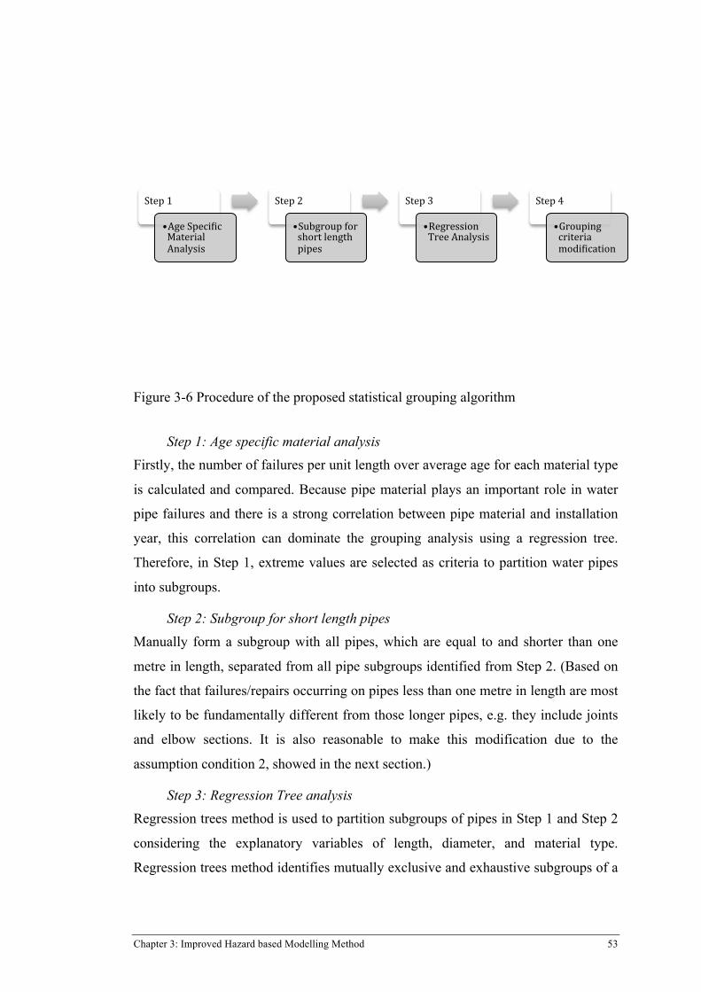
Chapter 3: Improved Hazard based Modelling Method 53
Figure 3-6 Procedure of the proposed statistical grouping algorithm
Step 1: Age specific material analysis Firstly, the number of failures per unit length over average age for each material type
is calculated and compared. Because pipe material plays an important role in water
pipe failures and there is a strong correlation between pipe material and installation
year, this correlation can dominate the grouping analysis using a regression tree.
Therefore, in Step 1, extreme values are selected as criteria to partition water pipes
into subgroups.
Step 2: Subgroup for short length pipes Manually form a subgroup with all pipes, which are equal to and shorter than one
metre in length, separated from all pipe subgroups identified from Step 2. (Based on
the fact that failures/repairs occurring on pipes less than one metre in length are most
likely to be fundamentally different from those longer pipes, e.g. they include joints
and elbow sections. It is also reasonable to make this modification due to the
assumption condition 2, showed in the next section.)
Step 3: Regression Tree analysis Regression trees method is used to partition subgroups of pipes in Step 1 and Step 2
considering the explanatory variables of length, diameter, and material type.
Regression trees method identifies mutually exclusive and exhaustive subgroups of a
Step 1
• Age Speci6ic Material Analysis
Step 2
• Subgroup for short length pipes
Step 3
• Regression Tree Analysis
Step 4
• Grouping criteria modi6ication

54 Chapter 3: Improved Hazard based Modelling Method
population, whose members share common characteristics that influence the
response variable of interest.
Step 4: Criteria modification The grouping criteria generated from Step 3 for length and diameter are in decimal
number, which sometimes is not reasonable. For example, there is no practical
meaning for a diameter equalling to 125.4mm. Therefore, a modification is needed to
round the decimal numbers.
Assumptions of the statistical grouping algorithm
(1) All work recorded in repair history is treated as failure records (e.g. ignoring the
possibility that a recorded work could actually be an inspection only.).
(2) One metre is used as the unit-length of a pipe in calculating the empirical hazard
(i.e. failure rate). The assumption is made such that no more than one repair will
occur at the same time to the same unit-length of a pipe. Even the repaired
unit-length may be “as good as new” (in the case of replacement that has
occurred), the whole pipe’s characteristic will still be considered “as bad as old”
for the repaired length, because this is normally much less than the total length.
(3) The empirical hazard distribution is defined as the age-specific failure rates. For
the water pipe case, the failure rate (or empirical hazard) is defined as
Number of failures per metre per year, which is calculated as
Repaired length of age-specific year divided by total length in operation at the beginning of the age-specific year.
The number of failures/repairs per unit length (with respect to each individual
pipe) is used as the statistical grouping criterion, which complies with the above
definition of age-specific failure rate.
3.3.2 A case study to test the proposed statistical grouping algorithm
The case study for testing the proposed statistical grouping algorithm is based on a
selected data set from a real water utility. Four types of materials (AC, DICL, CICL,
MS) for water pipes were selected.

Chapter 3: Improved Hazard based Modelling Method 55
Data used for statistical grouping algorithm
The data for grouping were given in two files:
1. Work order sheet: work order sheet recorded the failure/repair date of each
repair activity, and there were 3,400 sets of failure/repair records from 2002 to
2012;
2. Asset sheet: asset sheet recorded the general information of each pipe with pipe
length in metres, pipe diameter in millimetres, pipe materials, and pipe installed
date. The asset sheet consists of 40,653 sets of valid records.
(The raw data cannot be presented due to the need for confidentiality.)
Application Results
Step 1 outputs
The unit length in this case study is equal to 100m. Pipe material type is a major
factor or parameter in terms of grouping. From Step 1, the number of failures per
100m over average age for each material type was calculated, and was shown in
Figure 3-7. It can be observed from Figure 3-7 that DICL had the shortest average
life, and CICL had the longest average life. MS was considered as an outlier, because
it showed an extremely high value of failures/100m. This was caused by a fact that
one failure record and only 132.81 metres of pipe exist for this MS material in the
entire network. Thus MS will be excluded in the regression tree analysis in Step 2.
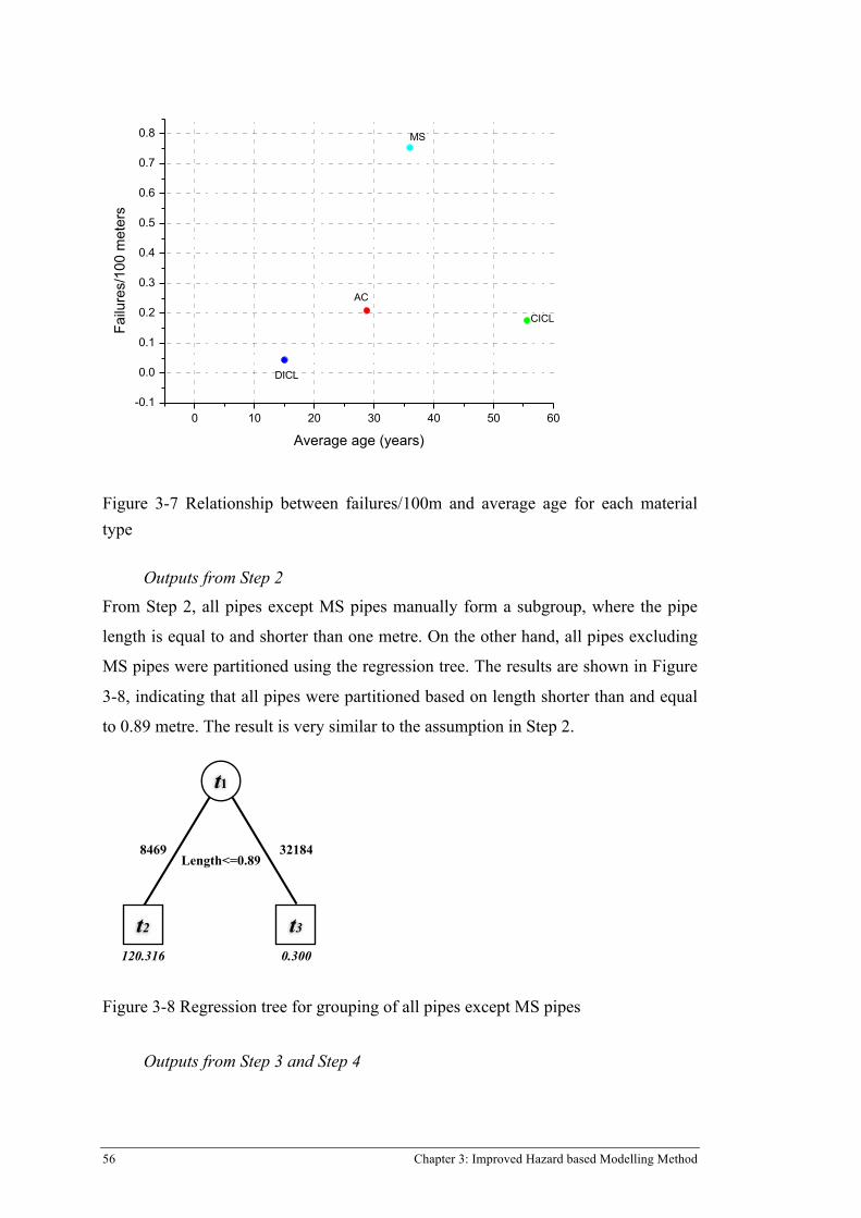
56 Chapter 3: Improved Hazard based Modelling Method
Figure 3-7 Relationship between failures/100m and average age for each material type
Outputs from Step 2
From Step 2, all pipes except MS pipes manually form a subgroup, where the pipe
length is equal to and shorter than one metre. On the other hand, all pipes excluding
MS pipes were partitioned using the regression tree. The results are shown in Figure
3-8, indicating that all pipes were partitioned based on length shorter than and equal
to 0.89 metre. The result is very similar to the assumption in Step 2.
Figure 3-8 Regression tree for grouping of all pipes except MS pipes
Outputs from Step 3 and Step 4
0 10 20 30 40 50 60-0.1
0.0
0.1
0.2
0.3
0.4
0.5
0.6
0.7
0.8Fa
ilure
s/10
0 m
eter
s
Average age (years)
MS
AC
CICL
DICL
t1
t2 t3
Length<=0.89
0.300
8469 32184
120.316
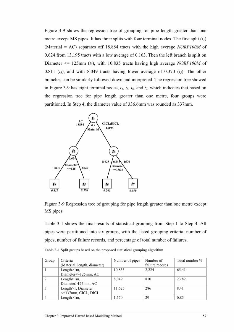
Chapter 3: Improved Hazard based Modelling Method 57
Figure 3-9 shows the regression tree of grouping for pipe length greater than one
metre except MS pipes. It has three splits with four terminal nodes. The first split (t1)
(Material = AC) separates off 18,884 tracts with the high average NORP100M of
0.624 from 13,195 tracts with a low average of 0.163. Then the left branch is split on
Diameter <= 125mm (t2), with 10,835 tracts having high average NORP100M of
0.811 (t3), and with 8,049 tracts having lower average of 0.370 (t5). The other
branches can be similarly followed down and interpreted. The regression tree showed
in Figure 3-9 has eight terminal nodes, t4, t5, t6, and t7, which indicates that based on
the regression tree for pipe length greater than one metre, four groups were
partitioned. In Step 4, the diameter value of 336.6mm was rounded as 337mm.
Figure 3-9 Regression tree of grouping for pipe length greater than one metre except MS pipes Table 3-1 shows the final results of statistical grouping from Step 1 to Step 4. All
pipes were partitioned into six groups, with the listed grouping criteria, number of
pipes, number of failure records, and percentage of total number of failures.
Table 3-1 Split groups based on the proposed statistical grouping algorithm
Group Criteria (Material, length, diameter)
Number of pipes Number of failure records
Total number %
1 Length>1m, Diameter<=125mm, AC
10,835 2,224 65.41
2 Length>1m, Diameter>125mm, AC
8,049 810 23.82
3 Length>1, Diameter <=337mm, CICL, DICL
11,625 286 8.41
4 Length>1m, 1,570 29 0.85
t1
t2
t4 t5 t6 t7
Material
Diameter<=125
0.811 0.370 0.263
AC18884
13195CICL;DICL
10835 8049
t3
Diameter<=336.6
11625 1570
0.019
0.3
0.6240.235

58 Chapter 3: Improved Hazard based Modelling Method
Diameter >337mm, CICL, DICL
5 Length<=1, all materials without MS
8,562 50 1.47
6 MS 12 1 0.03 Whole group 40,653 3,400 100
This case study only selected data with five materials; therefore, the failure records
for Group 4, Group 5 and Group 6 are not sufficient for hazard analysis. The
calculated empirical hazards in most of the ages are equal to “0”, which makes it
difficult to see the trends of the hazards in these groups through the calculated
empirical hazard values. Therefore, smoothed line patterns were calculated to show
the trends of hazard in each group, based on the Savitzky–Golay[112] smoothing
filter. The Savitzky–Golay[112] smoothing filter performs a local polynomial
regression on a series of values to determine the smoothed value for each point. In
this case study, a window size of 7 points is selected to smooth the empirical hazard
of Group 4 and Group 5. For Group 1 to Group 3, the failure records are sufficient;
therefore, empirical hazards were calculated for Group 1 to Group 3. Group 6 only
has one failure record, hence it is unable to show hazard trend, and therefore, it is
excluded in hazard analysis.
Figure 3-10 and Figure 3-11 show the empirical hazard for Group 1 to Group 3 as
well as the whole group, and smoothed line patterns for Group 4 and Group 5. It can
be seen that the empirical hazard curves and smoothed hazard curves between groups
are clearly distinctive from each other. The hazard curve of Group 5 in Figure 3-10
stands out due to its extraordinary short total length (hence resulting in some very
high empirical hazard values).

Chapter 3: Improved Hazard based Modelling Method 59
Figure 3-10 Empirical hazard and smoothed line patterns (Excluding Group 6)
Figure 3-11 Empirical hazard and smoothed line patterns (excluding Group 5 and Group 6)
0 10 20 30 40 50 60 70
0.0
5.0x10⁻⁴
1.0x10⁻³
1.5x10⁻³
2.0x10⁻³
2.5x10⁻³
3.0x10⁻³
3.5x10⁻³
4.0x10⁻³
Group3
Whole groups
Group5
Haz
ard
rate
(num
ber o
f fai
lure
s/m
etre
/yea
r)
Age (year)
Group1
0 10 20 30 40 50 60 70
0.0
2.0x10⁻⁴
4.0x10⁻⁴
6.0x10⁻⁴
8.0x10⁻⁴
Group4
Group2
Group3
Whole groups
Haz
ard
rate
(num
ber o
f fai
lure
s/m
etre
/yea
r)
Age (year)
Group1
60 Chapter 3: Improved Hazard based Modelling Method
From Figure 3-11, Group 1 shows higher values and more dramatically increasing
trend than other groups, which comply with the fact that AC pipes with small
diameters have higher a probability of failure than others. The hazard curve of Group
3 rises more dramatically than the curve of Group 4, which indicates that for CICL
and DICL pipes, larger diameter pipes have lower increasing trends than small
diameter pipes. By applying the statistical grouping algorithm, the hazard curves
between groups can be clearly separated from Group 1 to Group 5.
Given the above grouping results, it is recommended that the statistical grouping
algorithm applied in this research can be adopted as a general grouping methodology
in linear asset failure time data analysis.
3.4 THEORETIC FORMULAS OF EMPIRICAL HAZARDS, AND EVALUATION
Once all pipes in the network were partitioned into homogeneous groups with similar
characteristics based on the statistical grouping algorithm introduced in the previous
section, a theoretically sound and accurate empirical hazard function can be used
directly for analysis of life time distribution of the continuous-time failure data. This
section starts from clarifying the relationship between the concepts of hazard
function and failure rate. Then, two often-used continuous-time data empirical
hazard function formulas are derived directly from discrediting their theoretic
definitions of the hazard function. The properties of these two different formulas are
investigated and their estimation performances against the true hazard function
values are compared using simulation samples [113].
3.4.1 Introduction of empirical hazard function
Hazard function plays an essential role in the application of probability theory in
engineering reliability study. For example, the Mean Time To Failure (MTTF) is
calculated as the inverse of hazard rate if the asset system lifetime distribution is
assumed to follow an exponential distribution. In the data analysis stage, the term
failure rate is more often used when trying to work out the MTTF. Hazard or hazard
rate ℎ! ≡ ℎ(𝑡!) is the instantaneous failure rate at a time instant 𝑡! , 𝑖 = 1,2,⋯.
However, failure rate in data analysis is more often a short term for Average Failure
Rate (AFR) over a time period 𝑡! − 𝑡! (assuming 0 ≤ 𝑡! < 𝑡! ). AFR can be
calculated using formula [33]

Chapter 3: Improved Hazard based Modelling Method 61
AFR = ! ! !"!!
!!!!!!!
. (3-6)
Equation (3-6) is the average hazard function formula which is considered as the
most typical estimation of the true hazard function values [114]. Therefore, an
empirical hazard function formula is necessary, so that the hazard function h(t) can
be estimated based on observed sample data.
Sample failure time data can be treated as discrete data, i.e. the observed sample
failure times are considered as the events that occur at pre-assigned times 0 ≤ 𝑡! <
𝑡! < ⋯, and that under a parametric model of interest the hazard function at 𝑡! is
ℎ! = ℎ 𝑡! 𝜃 . A set of intervals 𝐼! = [𝑡! , 𝑡!!!) covering [0,∞) for an engineering
asset system is considered with N functional components at t1 = 0. Let 𝑑! = 𝑁 𝑡! −
𝑁 𝑡!!! , where 𝑁 𝑡! and 𝑁 𝑡!!! are the numbers of components, which are
functional at time 𝑡! and time 𝑡!!! , respectively. Then the quantity 𝑑! is the
number of failures in interval 𝐼!, and 𝑟! ≡ 𝑁 𝑡! is the number of components at
risk (i.e. having the potential to fail) at 𝑡!. It can be shown that the maximum
likelihood estimator (MLE) is
ℎ! =!!!! , (3-7)
from which the well-known Kaplan-Meier estimator for the reliability function
𝑅 𝑦 = (1− ℎ!)!:!!!! = 1− !!!!!:!!!! ,
is derived. Equation (3-7) is valid under independent right censoring [14, 115]. Note
that the Kaplan-Meier estimator is also valid for randomly censored data. For the
randomly censored data, the formula for the calculation of 𝑑! should be modified as
𝑑! = 𝑁 𝑡! − 𝑁 𝑡!!! − 𝑁! ! , (3-8)
where 𝑁!(!) is the number of components being censored in interval 𝐼!.
In data analysis practice, the sample failure time data is treated as continuous-time
data as shown in Equation (3-6). Two often-used empirical hazard function formulas
for treating the continuous-time data are:
62 Chapter 3: Improved Hazard based Modelling Method
ℎ! =! !! !! !!!∆!
∆!∙! !!= !
∆!!!!!≡ ℎ1!, (3-9)
and
ℎ! = − !∆!log 1− ! !! !! !!!∆!
! !!= − !
∆!log 1− !!
!!≡ ℎ2! , (3-10)
where ‘log’ represents the natural logarithm operation. The notation ∆𝑡 ≡ 𝑡!!! − 𝑡!
is used to emphasize that failures can happen at any time instants, not necessarily at
𝑡! , 𝑖 = 1,2,⋯ under the continuous-time data setting. The same cares need to be
taken in applying Equations (3-9) and (3-10), when calculating the empirical hazards
for the censored data. Equation (3-8) needs to be applied in calculating 𝑑!.
3.4.2 Empirical hazard function derivation and discussion
The following definition and relationship equations for the hazard function can be
found in any standard textbook on failure time data analysis. It is assumed that the
time to failure T is a random variable, which can take any value in the interval [0,∞).
The hazard function of T is defined as
ℎ 𝑡 = !(!)!!!(!)
= 𝑙𝑖𝑚∆!→!! !!∆! !!(!)∆!∙ !!!(!)
, (3-11)
where 𝑓(𝑡) and 𝐹(𝑡) are the pdf and cdf of T, respectively.
Since 𝑓 𝑡 = d𝐹(𝑡)/d𝑡, after further algebra, another form of the definition for the
hazard function is given as
ℎ 𝑡 = − ! !"# !!! !!!
= 𝑙𝑖𝑚∆!→!−!"# !!! !!∆! !!"# !!! !
∆!. (3-12)
By discretising Equations (3-11) and (3-12) respectively, the hazard function is given
as:
ℎ 𝑡 = ! !!∆! !! !∆!∙ !!! !
, (3-13)
and
ℎ 𝑡 = − !"# !!! !!∆! !!"# !!! !∆!
= − !∆!log !!! !!∆!
!!! !. (3-14)
Given the early defined notations N, 𝑁 𝑡! , ∆𝑡 ≡ 𝑡!!! − 𝑡! and ℎ! ≡ ℎ(𝑡!), the
relative frequency as the estimator for 𝐹 𝑡! is given as:
Chapter 3: Improved Hazard based Modelling Method 63
𝐹 𝑡! ≈ !!!(!!)!
= 1− ! !!!. (3-15)
By applying Equation (3-15) to Equations (3-13) and (3-14) accordingly, after some
algebras, Equations (3-9) and (3-10) are derived, where ‘log’ represents the natural
logarithm operation.
Up to this point, it is clear that both formulas (3-9) and (3-10) converge to the true
values of ℎ! as ∆𝑡 approaches zero. Note that this asymptotic property of
convergence still hold after the introduction of Equation (3-15) in the derivation
process due to the Law of large numbers [116]. The theoretic properties of formulas
(3-9) and (3-10) are investigated, when ∆𝑡 > 0. First, Equation (3-13) is rewritten as
ℎ 𝑡 =! ! !"!!∆!
!∆!
!!!! !
. (3-16)
Equation (3-16) implies that Equation (3-9) estimates the true hazard function values
by dividing the average density (!(!)!"!!∆!
!∆!
) over 1− 𝐹(𝑡), the system reliability
value at time t. This implies that Equation (3-9) will underestimate the true hazard
function values if the true density function (pdf) is decreasing over the interval ∆𝑡
and overestimate if the true pdf is increasing. Another way to show that Equation
(3-9) may be underestimating the true hi values is to consider ∆𝑡 as a unit time
interval, e.g. one hour, one day, or one year. Then, without loss of generality, the
empirical hazard function is given as:
ℎ! =𝑁 𝑡! − 𝑁 𝑡! + ∆𝑡
𝑁 𝑡!≡ ℎ1! .
Now Equation (3-14) is rewritten as
ℎ 𝑡 = ! !!∆! !!(!)∆!
, (3-17)
where 𝐻 𝑡 = ℎ(𝑢)d𝑢!! = −log (1− 𝐹(𝑡)) is the cumulative hazard function.
Equation (3-17) implies that Equation (3-10) calculates the average values of the true
hazard function. Therefore, Equation (3-10) will underestimate the true hazard
function during its decreasing stage and overestimate it during the true hazard
function's increasing stage. If the true hazard function is constant, Equation (3-10)
will give an unbiased estimation.

64 Chapter 3: Improved Hazard based Modelling Method
These theoretic properties of Equations (3-9) and (3-10) are verified by numeric
calculation results as shown in Figure 3-12, from which a further analysis to what
extent the bias of these two empirical hazards formulas is conducted. In Figure 3-12,
plots on the left column are the densities of the specified distributions (i.e.
exponential and Weibull); plots on the right column are the corresponding hazard
function values calculated based on the specified parameters. For exponential
distribution, the true hazards are calculated as:
ℎ 𝑡 = 𝜆,
where 𝜆 is a constant failure rate; For Weibull distribution, the true hazards are
given as:
ℎ 𝑡 = ! ! !
!!,
where 𝛼 and 𝛽 are the scale and shape parameters of the Weibull distribution.
In Figure 3-12, the top-down small triangle points indicates ℎ1! and the small
diamond points indicates ℎ2! , circle points are the true hazard function values
connected by a fine solid line. The rate of the exponential distribution has been
chosen to be 0.1 (plots in the first row); for Weibull distribution, shape = 3.5, scale =
60 for plots in row two; shape = 0.7, scale = 5 for plots in row three. The ℎ1! values
are calculated Equations (3-15); the ℎ2! values are calculated using Equation (3-17).

Chapter 3: Improved Hazard based Modelling Method 65
Figure 3-12 Investigation of the bias effects of the empirical hazard function values calculated using
ℎ1! and ℎ2!
Figure 3-12 shows that Equation (3-10) gives much less biased estimation of the true
hazard function than Equation (3-9). In particular, Equation (3-9) underestimates the
true hazard function values in most cases and the underestimation is substantial. On
the other hand, the bias created by Equation (3-10) is minor or none, if the fitted
model is an exponential distribution. Note that the extremely large underestimation
of the very first point in the bottom plots of Figure 3-12 is because the true hazard
value is positive infinity at 𝑡 = 0 (in the case of a Weibull distribution with shape
parameter less than one).
If 𝑡 + ∆𝑡 ≡ 𝑡! and 𝑡 ≡ 𝑡!, hence ∆𝑡 = 𝑡! − 𝑡!, Equation (3-6) and Equation (3-17)
are identical. This is how Equation (3-10) related to AFR but Equation (3-9) does not
have this direct connection.
As from Equation (3-11), the hazard function h(t), also referred to as hazard rate at
time t, is defined as a conditional density function, i.e. the ratio of probability density
𝑓(𝑡) over the reliability 1− 𝐹(𝑡) (a probability), which is not as intuitive to
interpret as the concept of failure rate used in data analysis. The direct connection of
0 20 40 60 80 100
0.00
00.
004
0.00
80.
012
xx
Expo
nent
ial d
ensit
ies
0 20 40 60 80
0.00
80.
010
0.01
2H
azar
ds
exponential(x|rate=0.01)
0 20 40 60 80 100
0.00
00.
010
0.02
0W
eibu
ll den
sitie
s
0 20 40 60 80
0.00
0.05
0.10
0.15
0.20
Haz
ards
Weibull(x|shape=3.5,scale=60)
0 20 40 60 80 100
0.0
0.1
0.2
0.3
0.4
failure times
Wei
bull d
ensit
ies
0 20 40 60 80
0.00
0.05
0.10
0.15
0.20
failure times
Haz
ards
Weibull(x|shape=0.7,scale=5)

66 Chapter 3: Improved Hazard based Modelling Method
Equation (3-10) with the AFR fills the mental gap between the probability theory and
data analysis.
Theoretically, the difference between formulas (3-9) and (3-10) is significant.
However, in data analysis practice, the numeric calculation results from both
formulas can be very close. As a standard mathematical result [116], it is known that,
if x ≤ 2/3, then
log 1+ 𝑥 = 𝑥 −𝑥!
2 + 𝜃 𝑥 ,
where θ(x) ≤ x !. Therefore, it is straight forward to show that if 0 < 𝑥 ≤ 0.1,
the relative difference between −log(1− 𝑥) and x (i.e. −log 1− 𝑥 − 𝑥 /
−log 1− 𝑥 ) is less than 6%.
A comparison of the estimation performances of Equations (3-9) and (3-10) to verify
the theoretic results was conducted in the next sections using the simulation failure
time data samples.
3.4.3 Comparison of empirical hazard function formulas using simulation samples
A random sample of an exponential distribution of sample size n=10000 is generated
with the parameter specification rate = 0.1 (using random seed 101 for exact
repeatability of the analysis results); A second random sample of a Weibull
distribution of sample size n = 10000 is generated with the parameter specification:
shape = 1.8 and scale = 30 (random seed = 101). Based on these two simulation
random samples, the empirical hazard values ℎ1! of Equation (3-9) and ℎ2! of
Equation (3-10) are calculated and compared with the true hazard function values to
verify the theoretic results obtained from Section 3.4.2.
Figure 3-13 presents the simulation results of comparing the empirical hazard values
ℎ1! and ℎ2! (invertical bars) against the true hazard function values (in circles
connected by a fine solid line) based on the exponential distribution random sample.
In calculating ℎ1! and ℎ2!, the most important setting is to specify the number of
intervals over the full sample data range. The specification of the number of intervals
is equivalent to specify the length of ∆𝑡. Therefore, it is expected to see the larger of
the number of intervals the better of the approximation of the ℎ1! and ℎ2! values
to the true hazard values. In Figure 3-13, the empirical hazards in the top two panel

Chapter 3: Improved Hazard based Modelling Method 67
plots are calculated using 20 intervals and in the bottom two panel plots the number
of intervals is 50. As concluded in Section 3.4.2, it is expected to see ℎ2! as an
unbiased estimator of the true hazard function and that ℎ1! will underestimate. The
graph shows that ℎ2! always performs better than ℎ1! , which is consistently
underestimating the true hazards. The difference is much more significant when the
number of intervals is small. It is also noticed that it is ℎ1! , which is much more
sensitive to the number of intervals specification, while ℎ2! 's estimation results are
very robust (i.e. almost not affected by the change of the number of intervals
specification).
Figure 3-13 Empirical hazard function values calculated using ℎ1! (the top and third panel plots) and
ℎ2!(the second and bottom panel plots)
With this particular exponential distribution sample, the 99% quantile value is about
45 time units, which is spread over less than 60% of the full sample data range. Note
that, for both ℎ1! and ℎ2!, the estimates fluctuate wildly after the 99% quantile
point because of the sparseness of observations over the upper part of the range
interval. Actually, ℎ2! will always have an infinite large hazard value for the last
interval because it is imagined all components must fail in the end. On the other hand,
ℎ1! will always be equal to 1/∆𝑡 for the last interval; thus, empirical values of the
0 20 40 60 80
0.00
0.10
haza
rd
exponential(x|rate=0.1)
0 20 40 60 80
0.00
0.10
haza
rd
0 20 40 60 80
0.00
0.10
haza
rd
0 20 40 60 80
0.00
0.10
failure times
haza
rd

68 Chapter 3: Improved Hazard based Modelling Method
very last interval should not be included. Therefore, only the estimates calculated
from those sample observations are utilised, which are up to 99% quantile point.
Figure 3-14 Empirical hazard function values calculated using ℎ1! (top panel plot) and ℎ2! (bottom
panel plot)
Figure 3-14 examines the simulation results of comparing the empirical hazard
values ℎ1! (top panel) and ℎ2! (bottom panel) against the true hazard function
values based on a Weibull distribution random sample. Figure 3-14 follows the same
drawing convention as in Figure 3-13, i.e. the empirical hazard values ℎ1! and ℎ2!
are represented in vertical bars against the true hazard function values (in circles
connected by a fine solid line). The number of intervals is chosen to be 45, i.e. ∆t =
2 time units. In addition, the approximate 95% confidence bands for ℎ1!and ℎ2!
values are constructed using the parametric bootstrap method [117]. Based on the
Weibull distribution specification, 500 bootstrap samples (each of n* = 10000) are
generated and ℎ1! and ℎ2! are calculated for each of these bootstrap samples. The
medians of empirical hazards are superimposed using a thick (in blue colour) solid
line with the dashed lines (in grey colour) for the lower and upper limits respectively.
0 20 40 60 80
0.00
0.10
0.20
0.30
haza
rd
Weibull(x|shape=1.8,scale=30): complete sample
0 20 40 60 80
0.00
0.10
0.20
0.30
failure times
haza
rd

Chapter 3: Improved Hazard based Modelling Method 69
Based on the theoretic results obtained in Section 3.4.2, ℎ1!will overestimate when
failure times are small and underestimate when failure times become larger; ℎ2!
will overestimate slightly the true hazards. In Figure 3-14, the overestimation effect
of ℎ1! and the overestimation effects of ℎ2! are visually unidentifiable. In contrast,
the underestimation effect of ℎ1! is substantial. In addition, in this particular
Weibull distribution sample, the 99% quantile point is at about 70 time units. In
Figure 3-14, the superimposed confidence bands show how much the sampling
variation can be over the upper part of the sample data range.
The results in this section have shown that ℎ2! (defined in Equation (3-10)) is
nothing but a finite approximation of AFR, whereas ℎ1! (defined in Equation (3-9))
is a finite approximation of the instantaneous hazard rates. However, in their limiting
forms, both ℎ1!and ℎ2! converge to the true hazard function ℎ!.
For data analysis purposes, a rule of thumb for calculating empirical hazard function
of continuous-time failure data may be summarised as: if the maximum failure rate
over the time interval periods is less than 0.1, both ℎ1! and ℎ2! are good
estimators of the true hazard function values. Most asset management reliability
study cases should fall into this category. Otherwise, ℎ2! should be used for
calculating the empirical hazard function.
Note that both formulas are valid for randomly censored continuous-time failure data.
In this section, it is necessary to concentrate on discussing the calculation of the
complete failure time data using simulation samples.
3.5 HAZARD MODELLING FOR TRUNCATED LIFETIME DATA OF WATER PIPES
3.5.1 The real situation of lifetime data for water pipes
In reality, lifetime data for water pipes often contain a great proportion of truncated
data. For a real water utility, the overwhelming majority of the water pipes may be
right censored, because of a water pipe’s long useful life, i.e. most of the pipes (more
than 90%) may never have any repairs that have occurred during the observation
period. The lifetime of water pipe segments showed different scenarios, which are
illustrated in Figure 3-15.

70 Chapter 3: Improved Hazard based Modelling Method
Figure 3-15 Schematic of lifetime distribution of water pipe segment in calendar time In Figure 3-15, the following schema is used: the horizontal axis indicates the time
line of calendar year, which starts from the year that the first pipe installed. Here,
1920 is set as an example. Each horizontal line indicates the lifetime of each pipe
segment from its installation date to its repair date. Pipe segments represented by
horizontal lines with little vertical bars on their left ends are for the known
installation date cases; small circles representing the installation dates were missing.
The small solid cube signs are marked on the right end of the line segment for
indicating the repair date, again, a small circle representing the repair dates is
missing. The two vertical lines with year 2002 and 2012 illustrate that the
observation period is from 2002 to 2012. If the right ends of a pipe segment run
beyond the 2012 line, this is the right-censored case. Therefore, in summary, pipe
cases marked with ‘1’ are the right censored data; pipe cases marked with ‘0’ are the
data with repair records; pipe cases marked with ‘2’ are the data with unknown
installation date but repairs observed; pipe cases marked with ‘3’ are the right
censored data but with unknown installation date; finally, pipe segment cases marked
with ‘4’ are the missing value data of which researchers may not even be aware.
Given the fact that the number of data with unknown installation dates is so few,
these data are treated as missing value data and exclude them before starting the
empirical hazards calculation. In order to calculate the age-specific empirical hazard
values, firstly the observations are needed to be synchronised. Note also, even with
00
0
0
11
1
11
13
11
1
14
4
3
2
1920 2002 2012 Calendar year

Chapter 3: Improved Hazard based Modelling Method 71
those pipes which have been repaired, the pipes still exist so that they must be
included as part of the total length pipes in operation. Figure 3-16 gives the
schematic illustration of the situation.
Figure 3-16 Schematic of lifetime distribution of water pipes (age-specific) In Figure 3-16 the horizontal axis indicates the time line of age in year, which starts
from “0”. Each horizontal line indicates the lifetime of each pipe from age “0” to the
age when it is repaired. The vertical line with age 70 illustrates the observation
period for the longest age of pipes. For pipes marked with “1”, this indicates the right
censored situation, where their ages are longer than the longest observed age of pipes.
The pipes marked with “2” and “3” do not retain any information of their installation
data; therefore, their ages are unknown. It is impossible to calculate the empirical
hazard based on age, therefore, these two types of pipes are treated as invalid data.
The pipes marked with “0” are the pipes with failure/repair history records.
Pipes marked with “4” cannot be observed and it is impossible to know how many
pipes are in this scenario and which pipe falls into this scenario. Therefore, in the
interval truncated observation, pipes in scenario “4” can only be treated as the pipes
in scenario “1”. In Section 3.4.1, 𝑟! is the length of pipe segments at risk at 𝑡!,
𝑟! ≡ 𝑁 𝑡! . If pipes in scenario “4” are treated as pipes in scenario “1”, 𝑟! will be
00
0
0
111
111
111
14
4
3
2
0 age (year)
3
10 20 30 40 50 60 70

72 Chapter 3: Improved Hazard based Modelling Method
greater than its original values. Therefore, using Equation (3-9) or Equation (3-10),
the calculated empirical hazard will underestimate the true hazard value.
In the next section, a modified empirical hazard function to deal with the interval
truncated lifetime data is developed in order to reduce the underestimation of hazard.
3.5.2 Empirical hazard function for interval truncated lifetime data
In section 3.4.2, two empirical hazard functions were introduced in Equation (3-9)
and Equation (3-10) given as:
ℎ! =! !! !! !!!∆!
∆!∙! !!= !
∆!!!!!≡ ℎ1!,
and
ℎ! = − !∆!log 1− ! !! !! !!!∆!
! !!= − !
∆!log 1− !!
!!≡ ℎ2! .
𝑑! indicates the length of repaired pipe in the interval between time instant 𝑡! and
𝑡!!!,𝑖 = 1,2,…, where 𝑑! = 𝑁 𝑡! − 𝑁 𝑡!!! .
𝑟! ≡ 𝑁 𝑡! , (3-18)
is the length of pipe segments at risk at 𝑡!. 𝑁 𝑡! and 𝑁 𝑡!!! are the length of
pipes which are functional at time 𝑡! and time 𝑡!!!, respectively, where 𝑡! and
𝑡!!! indicate a pipe’s age in year units.
For the interval truncated lifetime data, a truncated time interval is given as (𝐿! ,𝑅!].
The length of pipes’ survival at time 𝐿! and 𝑅! are given as 𝑁 𝐿! and 𝑁 𝑅! ,
respectively. The length of pipes repaired in the time interval (𝐿! ,𝑅!] can be
denoted as 𝑁!", which can be calculated by 𝑁!" = 𝑁 𝑅! − 𝑁 𝐿! .
As introduced before, water pipe as a linear asset can be treated as a number of
unit-length segments, and each repair is replacing the pipe segment. Compared with
the length of pipe, the length of each segment is far smaller than the whole pipe,
therefore, the condition of the whole pipe after each repair can still remain “as bad as
old”, even if the condition of each repaired segment is “as good as new”. Therefore,
an assumption is made that the condition of these repaired pipe segments in
unit-length 𝑁!" can be treated “as good as new”. These repaired pipe segments are
treated as additional new pipe segments, and a new asset table is created for the new
pipe segments. Therefore the new pipe length at time 𝑡! is given by 𝑁!"#(𝑡!).
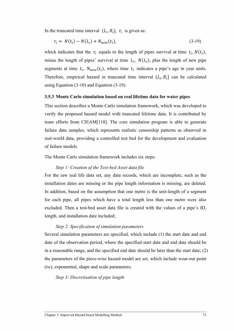
Chapter 3: Improved Hazard based Modelling Method 73
In the truncated time interval (𝐿! ,𝑅!], 𝑟! is given as:
𝑟! = 𝑁 𝑡! − 𝑁 𝐿! + 𝑁!"#(𝑡!), (3-19)
which indicates that the 𝑟! equals to the length of pipes survival at time 𝑡!, 𝑁 𝑡! ,
minus the length of pipes’ survival at time 𝐿!, 𝑁 𝐿! , plus the length of new pipe
segments at time 𝑡!, 𝑁!"#(𝑡!), where time 𝑡! indicates a pipe’s age in year units.
Therefore, empirical hazard in truncated time interval (𝐿! ,𝑅!] can be calculated
using Equation (3-10) and Equation (3-19).
3.5.3 Monte Carlo simulation based on real lifetime data for water pipes
This section describes a Monte Carlo simulation framework, which was developed to
verify the proposed hazard model with truncated lifetime data. It is contributed by
team efforts from CIEAM[118]. The core simulation program is able to generate
failure data samples, which represents realistic censorship patterns as observed in
real-world data, providing a controlled test bed for the development and evaluation
of failure models.
The Monte Carlo simulation framework includes six steps:
Step 1: Creation of the Test-bed Asset data file For the raw real life data set, any data records, which are incomplete, such as the
installation dates are missing or the pipe length information is missing, are deleted.
In addition, based on the assumption that one metre is the unit-length of a segment
for each pipe, all pipes which have a total length less than one metre were also
excluded. Then a test-bed asset data file is created with the values of a pipe’s ID,
length, and installation date included;
Step 2: Specification of simulation parameters Several simulation parameters are specified, which include (1) the start date and end
date of the observation period, where the specified start date and end date should be
in a reasonable range, and the specified end date should be later than the start date; (2)
the parameters of the piece-wise hazard model are set, which include wear-out point
(tw), exponential, shape and scale parameters;
Step 3: Discretisation of pipe length

74 Chapter 3: Improved Hazard based Modelling Method
Each pipe is broken down into a number of independent unit-length (one-metre)
segments for modelling purposes, assuming that all the one-metre segments have the
same failure rate.
Step 4: Generation of lifetime distribution before the wear-out point (tw)
Based on the input value of the exponential parameter, lifetime for each segment is
generated. If the lifetime is equal to or smaller than the value of tw, the lifetime value
will be saved for that segment. For those segments with lifetimes larger than the
values of tw, the lifetimes are temporarily saved and the simulation moves on to Step
5.
Step 5: Generation lifetime distribution after the wear-out point (tw) For those segments temporarily saved in Step 4, new lifetimes were generated based
on the input values of the shape and scale parameters. The new lifetime is compared
with the temporarily saved lifetime for each segment, and the smaller one is saved as
the final lifetime.
Step 6: Selection of segments for their failure date in the observation period
The age-specified lifetimes were transferred to the time scales of calendar years
based on the installation dates in the test-bed asset data file. Then, the segments,
whose lifetimes are located in the observation period (defined by the start and end
date), are selected and saved in a failure record file. The procedure will be terminated
if all pipes are treated, then the saved failure record file is the simulated failure
record for the whole water pipe network; otherwise, the simulation moves back to
Step 3.
3.5.4 Validation of the proposed empirical hazard function
In this section, the test-bed sample data based on the Monte Carlo simulation is
implemented to test and validate the proposed empirical hazard function of truncated
lifetime data. The truncation period is determined by the start date and end date in
the Monte Carlo simulation. The improvements based on Equation (3-19) on the
installation data distribution and pipe length distribution of water pipes are conducted
and analysed with the following examples.
Example 1:
In Example 1, parameters are shown in Table 3-2, where 𝜆 is a constant failure rate,
𝜉 indicates the start time, 𝛼 and 𝛽 are the scale and shape parameters of the

Chapter 3: Improved Hazard based Modelling Method 75
Weibull distribution in Equation (3-1). The “Observation period” indicates the
observation starting at 01/07/2002 and finishing at 30/06/2012.
Table 3-2 Parameters for Example 1 𝜉 𝜆 𝛽 𝛼 Observation period 15 0.0001 1.5 370 01/07/2002 to 30/06/2012
In Figure 3-17, the top chart shows the hazards with age in years based on Equation
(3-18), the red bar shows the empirical hazard, and the blue solid line indicates the
true hazard; The meddle chart indicates the length distribution in kilometres and the
bottom chart shows number of repairs with age in years.
Figure 3-17 The goodness-of-fit of empirical hazards vs. the true hazard based on Equation (3-18) Figure 3-18 shows the hazards with age in years based on Equation (3-19). The
hazard plot in Figure 3-18 is almost a perfect fit compared with the hazard plot in
Figure 3-17, which shows a fundamental improvement over the old way of
calculating the empirical hazards.
0 20 40 60
0.00
00.
002
0.00
4H
azar
ds
Goodness-of-fit of empirical hazards vs theoretic/true hazards
0 20 40 60
010
0020
0030
00T
otal
Len
gth
in k
m
0 20 40 60
020
040
060
080
0
Age in years
# of
rep
airs
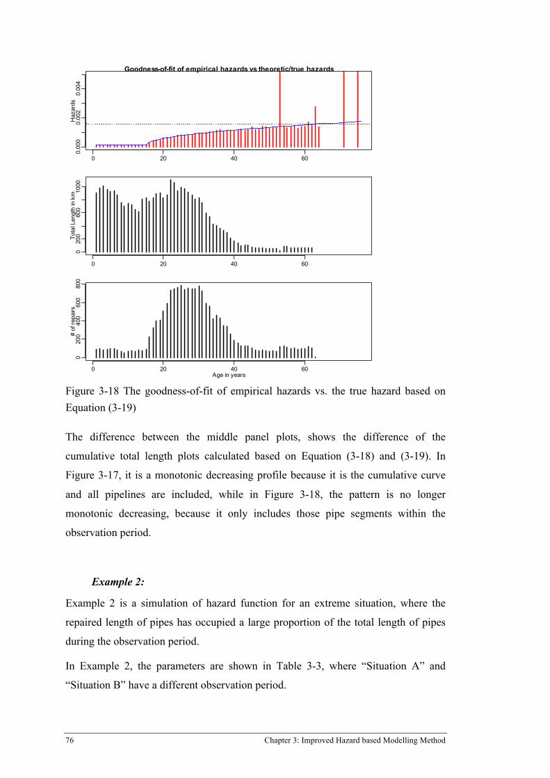
76 Chapter 3: Improved Hazard based Modelling Method
Figure 3-18 The goodness-of-fit of empirical hazards vs. the true hazard based on Equation (3-19) The difference between the middle panel plots, shows the difference of the
cumulative total length plots calculated based on Equation (3-18) and (3-19). In
Figure 3-17, it is a monotonic decreasing profile because it is the cumulative curve
and all pipelines are included, while in Figure 3-18, the pattern is no longer
monotonic decreasing, because it only includes those pipe segments within the
observation period.
Example 2:
Example 2 is a simulation of hazard function for an extreme situation, where the
repaired length of pipes has occupied a large proportion of the total length of pipes
during the observation period.
In Example 2, the parameters are shown in Table 3-3, where “Situation A” and
“Situation B” have a different observation period.
0 20 40 60
0.00
00.
002
0.00
4H
azar
dsGoodness-of-fit of empirical hazards vs theoretic/true hazards
0 20 40 60
020
060
010
00To
tal L
engt
h in
km
0 20 40 60
020
040
060
080
0
Age in years
# of
repa
irs

Chapter 3: Improved Hazard based Modelling Method 77
Table 3-3 Parameters for Example 2 𝜉 𝜆 𝛽 𝛼 Situation A Situation B
10 0.0001 1.1 49 Earliest installed date to 30/06/2012
01/07/2002 to 30/06/2012
Figure 3-19 and Figure 3-20 are in the same structure of Figure 3-17 in that the top
chart shows the hazards with age in years, the middle chart shows the total length
distribution in kilometres, and the bottom chart shows the number of repairs with age
in years.
Figure 3-19 The goodness-of-fit of empirical hazards vs. the true hazard in Situation A based on Equation (3-18) The hazard plot in Figure 3-20 is almost a perfect fit compared with the hazard plot in Figure 3-19, which shows a fundamental improvement over the old way of calculating the empirical hazards. The difference between the middle panel plots shows the difference of the cumulative total length plots calculated based on Equation (3-18) and (3-19).
0 20 40 60
0.00
00.
010
0.02
00.
030
Haz
ards
Goodness-of-fit of empirical hazards vs theoretic/true hazards
0 20 40 60
010
0020
0030
00To
tal L
engt
h in
km
0 20 40 60
010
000
3000
0
Age in years
# of
repa
irs
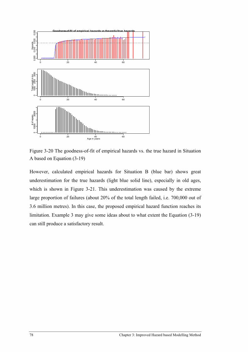
78 Chapter 3: Improved Hazard based Modelling Method
Figure 3-20 The goodness-of-fit of empirical hazards vs. the true hazard in Situation A based on Equation (3-19) However, calculated empirical hazards for Situation B (blue bar) shows great
underestimation for the true hazards (light blue solid line), especially in old ages,
which is shown in Figure 3-21. This underestimation was caused by the extreme
large proportion of failures (about 20% of the total length failed, i.e. 700,000 out of
3.6 million metres). In this case, the proposed empirical hazard function reaches its
limitation. Example 3 may give some ideas about to what extent the Equation (3-19)
can still produce a satisfactory result.
0 20 40 60
0.00
00.
010
0.02
00.
030
Haza
rds
Goodness-of-fit of empirical hazards vs theoretic/true hazards
0 20 40 60
010
0020
0030
00To
tal L
engt
h in
km
0 20 40 60
010
000
3000
0
Age in years
# of
repa
irs
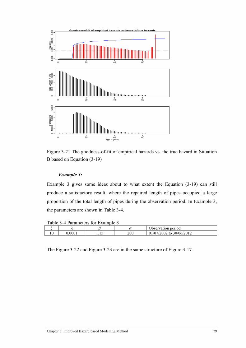
Chapter 3: Improved Hazard based Modelling Method 79
Figure 3-21 The goodness-of-fit of empirical hazards vs. the true hazard in Situation B based on Equation (3-19)
Example 3:
Example 3 gives some ideas about to what extent the Equation (3-19) can still
produce a satisfactory result, where the repaired length of pipes occupied a large
proportion of the total length of pipes during the observation period. In Example 3,
the parameters are shown in Table 3-4.
Table 3-4 Parameters for Example 3 𝜉 𝜆 𝛽 𝛼 Observation period 10 0.0001 1.15 200 01/07/2002 to 30/06/2012
The Figure 3-22 and Figure 3-23 are in the same structure of Figure 3-17.
0 20 40 60
0.00
00.
010
0.02
00.
030
Haza
rds
Goodness-of-fit of empirical hazards vs theoretic/true hazards
0 20 40 60
010
0020
0030
00To
tal L
engt
h in
km
0 20 40 60
010
000
3000
050
000
Age in years
# of
repa
irs
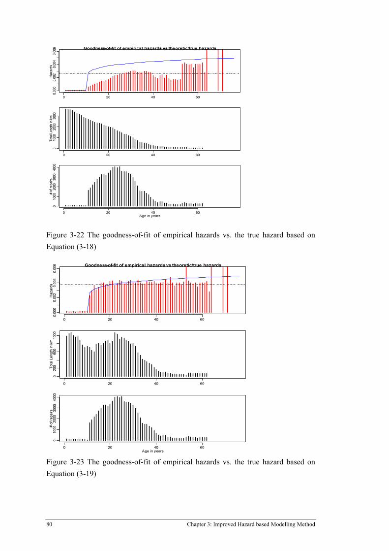
80 Chapter 3: Improved Hazard based Modelling Method
Figure 3-22 The goodness-of-fit of empirical hazards vs. the true hazard based on Equation (3-18)
Figure 3-23 The goodness-of-fit of empirical hazards vs. the true hazard based on Equation (3-19)
0 20 40 60
0.00
00.
002
0.00
40.
006
Haza
rds
Goodness-of-fit of empirical hazards vs theoretic/true hazards
0 20 40 60
010
0020
0030
00To
tal L
engt
h in
km
0 20 40 60
010
0020
0030
0040
00
Age in years
# of
repa
irs
0 20 40 60
0.00
00.
002
0.00
40.
006
Haz
ards
Goodness-of-fit of empirical hazards vs theoretic/true hazards
0 20 40 60
020
060
010
00To
tal L
engt
h in
km
0 20 40 60
010
0020
0030
0040
00
Age in years
# of
repa
irs

Chapter 3: Improved Hazard based Modelling Method 81
In Example 3, the number of failures generated by the simulation is about 88,000. In
practice, this great number of failures is a pretty ‘bad’ case, which is hardly
happened in real life. Compared with the hazard plots in Figure 3-22 and Figure 3-23,
Equation (3-19) still can handle well, compared with Equation (3-18). Therefore, the
calculated empirical hazards based on Equation (3-10) and (3-19) are good
estimations of the true hazards based on the simulation experiments, which can be
applied for most of the failure scenarios for water pipes.
3.5.5 Hazard distribution fitting method for the piece-wise hazard model
Parameters of the piece-wise hazard model can be estimated by non-linear regression.
However, there is a limitation that the wear-out point needs to be estimated by expert
knowledge; Therefore, in this section, a hazard distribution fitting method is
developed.
To automatically estimate the optimal wear-out point (tw), an equation to calculate
the error between the empirical hazard and the fitted hazard of a given 𝑡𝑤 is given
as:
𝑅!" = ℎ 𝑡 − ℎ!"# 𝑡, 𝑡𝑤!"#(!)!!! , (3-20)
where ℎ 𝑡 indicates the empirical hazard at age t, and ℎ!"# 𝑡, 𝑡𝑤 indicates the
fitted hazard at age t with a value of 𝑡𝑤. ℎ!"# 𝑡, 𝑡𝑤 is calculated by the non-linear
regression introduced in Section 3.2, based on a given 𝑡𝑤. 𝑡𝑤 = 1,2,…max (𝑡),
where the max (𝑡) is normally lower than 100.
In the fitting method, 𝑡𝑤 is given from 1 to the max (𝑡). For each given 𝑡𝑤, the
non-linear regression is used to estimate the parameters of 𝜆, 𝛽, and 𝛼 in Equation
(3-1). Then the objective is to find the optimal 𝑡𝑤, which let the 𝑅!" have a
minimum value, so that the optimal wear-out point (𝑡𝑤) is estimated.
This fitting method is verified by the simulation samples in Example 1 applied in
Section 3.5.4. In Figure 3-24, the blue line is the true hazard function values; the
vertical bars are the medians of the empirical hazard function values calculated from
100 bootstrap samples; the two black dashed lines are the approximate 95%
confidence band; the red circle points are the medians of the fitted hazard values
connected by a fine solid line, which is calculated from 100 bootstrap samples; the
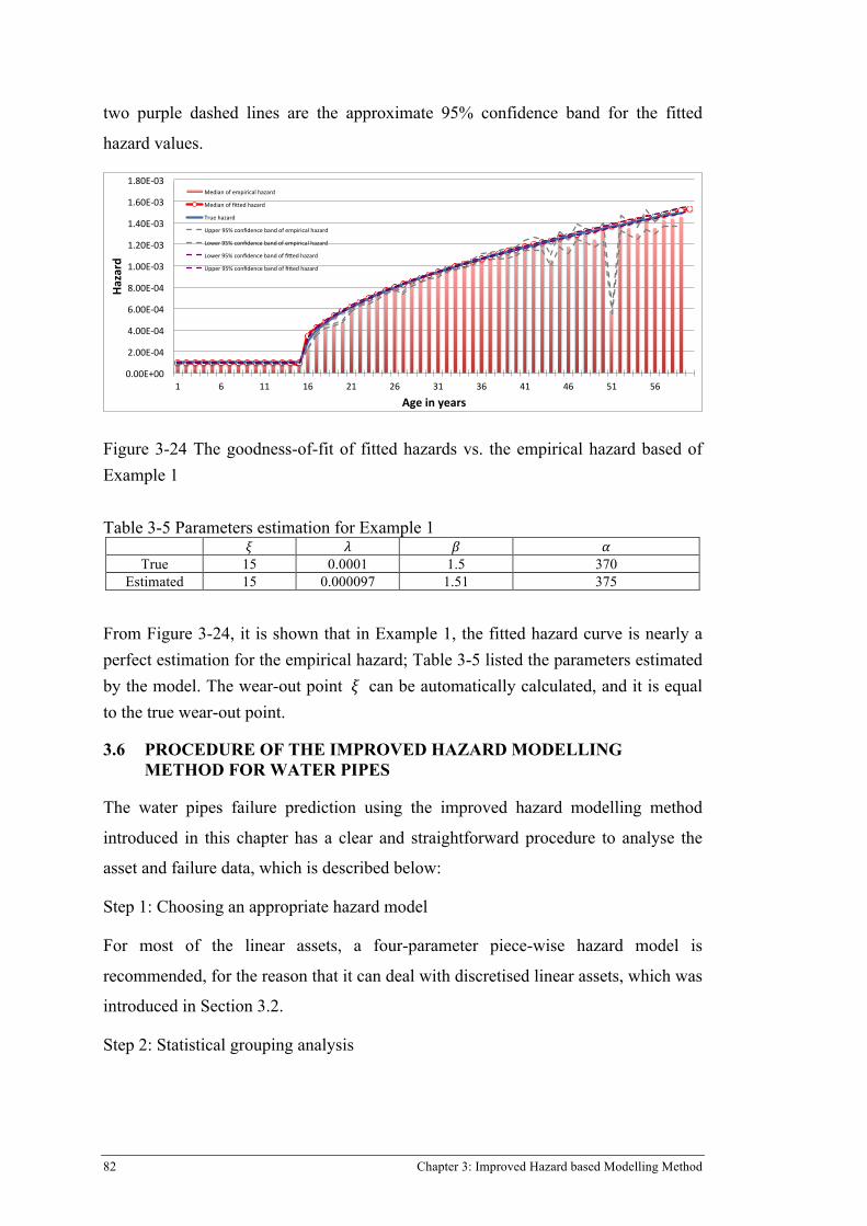
82 Chapter 3: Improved Hazard based Modelling Method
two purple dashed lines are the approximate 95% confidence band for the fitted
hazard values.
Figure 3-24 The goodness-of-fit of fitted hazards vs. the empirical hazard based of Example 1 Table 3-5 Parameters estimation for Example 1
𝜉 𝜆 𝛽 𝛼 True 15 0.0001 1.5 370
Estimated 15 0.000097 1.51 375
From Figure 3-24, it is shown that in Example 1, the fitted hazard curve is nearly a perfect estimation for the empirical hazard; Table 3-5 listed the parameters estimated by the model. The wear-out point 𝜉 can be automatically calculated, and it is equal to the true wear-out point.
3.6 PROCEDURE OF THE IMPROVED HAZARD MODELLING METHOD FOR WATER PIPES
The water pipes failure prediction using the improved hazard modelling method
introduced in this chapter has a clear and straightforward procedure to analyse the
asset and failure data, which is described below:
Step 1: Choosing an appropriate hazard model
For most of the linear assets, a four-parameter piece-wise hazard model is
recommended, for the reason that it can deal with discretised linear assets, which was
introduced in Section 3.2.
Step 2: Statistical grouping analysis
0.00E+00%
2.00E'04%
4.00E'04%
6.00E'04%
8.00E'04%
1.00E'03%
1.20E'03%
1.40E'03%
1.60E'03%
1.80E'03%
1% 6% 11% 16% 21% 26% 31% 36% 41% 46% 51% 56%
Hazard�
Age)in)years�
Median%of%empirical%hazard%
Median%of%fi>ed%hazard%
True%hazard%
Upper%95%%confidence%band%of%empirical%hazard%
Lower%95%%confidence%band%of%empirical%hazard%
Lower%95%%confidence%band%of%fi>ed%hazard%
Upper%95%%confidence%band%of%fi>ed%hazard%

Chapter 3: Improved Hazard based Modelling Method 83
Pipe data should be partitioned based on their characteristic features using the
statistical grouping algorithm. The four-step grouping procedure should be followed
for partitioning pipes, which was developed in Section 3.3. Then the final groups and
the grouping criteria can be acquired.
Step 3: Choosing empirical hazard function
The empirical hazard function of Equation (3-10) is recommended for all
circumstances. However, if the failure rate is less than 0.1, both Equation (3-9) and
Equation (3-10) will be appropriate for calculating empirical hazard.
Step 4: Calculating empirical hazard values based on the modified empirical hazard
model
For real life data, Equation (3-19) combined with Equation (3-10) is recommended
for calculating empirical hazard values in order to reduce the underestimation effects.
Step 5: Estimating the model parameters based on empirical hazard values
To estimate the model parameters, MLE or regression methods can be used based on
the hazard models. For the piece-wise hazard model, the non-linear regression
method can be applied to calculate the four parameters.
3.7 SUMMARY
This chapter described an improved hazard modelling method for water pipes. The
development of this model includes three components. The first component is a
statistical grouping algorithm using a four-step procedure, which combines age
specific material analysis, length related pre-grouping, regression tree analysis, and
grouping criteria adjustment based on knowledge rules. The result of a case study
showed that, by applying this procedure, pipe data can be partitioned into more
homogeneous groups, and sufficient sample size of failure data for each group can be
guaranteed.
The second component is a comparison study of two commonly used empirical
hazard formulas ℎ1! and ℎ2! (Equations (3-9) and (3-10)) for investigating their
differences of application impacts. The differences were tested using simulation
samples from exponential and Weibull distributions. The investigation of the
empirical hazard formulas for linear assets draws the following conclusions: (1) ℎ1!
is a finite approximation of the instantaneous failure rate, and it underestimates the
84 Chapter 3: Improved Hazard based Modelling Method
true hazard function values in most cases and the underestimation is substantial; and
the underestimation of ℎ1! is much more sensitive to the change of time interval ∆𝑡;
(2) ℎ2! is a finite approximation of average failure rate (AFR), and it gives a much
less biased estimation of the true hazard function than ℎ1! ; ℎ2! is almost not
affected by the change of time interval ∆𝑡. (3) For calculating empirical hazard
function of continuous-time failure data, if the maximum failure rate over the time
interval periods is less than 0.1, both formulas are good estimators of the true hazard
function values. Otherwise, ℎ2! has more accuracy of result than ℎ1! for
calculating the empirical hazard function.
The third component is a modified empirical hazard function to deal with the
underestimation effects due to interval truncated lifetime data by considering three
types of pipe segments: survived segments, repaired segments and new segments. A
Monte Carlo simulation framework has been developed in order to generate test-bed
sample data sets in terms of the main features of the real data of a water utility.
Based on the simulation results, the modified empirical hazard function can
effectively reduce the underestimation effects caused by the interval truncation of
lifetime data.
By applying the improved hazard modelling method for water pipe reliability
analysis, the hazard curves between groups can be clearly distinctive from each other;
and the underestimation effects caused by interval truncated lifetime data can be
reduced; hence, more accurate hazard prediction results for each group of pipes can
be calculated.

Chapter 4: Optimization Model of Group Replacement Schedules for Water Pipelines 85
Chapter 4: Optimization Model of Group Replacement Schedules for Water Pipelines
4.1 INTRODUCTION
Replacement of water pipeline is crucial to water utilities due to the deterioration of
water pipes, especially those that are aged. Not only does replacement contribute to
the service with quality, but also enriches all the company experience surrounding
the service provided[119]. Huge investment pressures of water pipe maintenance has
led to the improvements of replacement efficiency and cost effectiveness.
Researchers have provided various replacement decision support models [6, 8, 11,
12].
In current practice, replacement activities are usually scheduled into groups manually.
However, this practice fails to provide an optimal solution because it relies on users’
experiences. Optimal group scheduling needs to take into consideration of multiple
criteria such as costs, impact of service interruptions, pipe specifications, the type of
technology employed and geographical information. However, replacement group
scheduling for individual water pipes considering multiple criteria has so far not
received enough attention in literature.
To improve the existing replacement scheduling, an innovative decision model,
Replacement Decision Optimization Model for Group Scheduling (RDOM-GS), is
proposed in this chapter. This model provides planners unambiguous information for
optimizing group replacement scheduling for groups of water pipelines. This model
enables planners to develop group replacement schedules against three criteria:
shortest geographic distance, maximum replacement equipment utilization, and
minimum service interruption. The RDOM-GS integrates cost analysis, service
interruption analysis, and optimization analysis to deliver schedules that limit service
interruptions and minimize total life-cycle cost.
The rest of the chapter starts with water pipeline maintenance with the economics of
repair and replacement in Section 4.2. Then, in Section 4.3, cost functions for water
pipeline repair and replacement are introduced and developed, based on the hazard

86 Chapter 4: Optimization Model of Group Replacement Schedules for Water Pipelines
model developed in Chapter 3. In Section 4.4, replacement group scheduling criteria
are introduced, followed by a judgment matrix and three integrated models for
replacement group scheduling. A new replacement cost function for group
scheduling is developed in Section 4.5, followed by a customer service interruption
model in Section 4.6. The objectives and constrains for RDOM-GS are summarized
in Section 4.7. Finally, the structure of the RDOM-GS is summarised in Section 4.8.
4.2 MAINTENANCE ON WATER PIPELINES
4.2.1 Repair and replacement of water pipeline
Maintenance plays an essential role in asset management to improve the reliability of
system. There are two basic categories of maintenance [33], corrective maintenance
and preventive maintenance. Corrective maintenance follows in-service failures to
restore the system to its operational state through corrective action, and nothing is
done before the system fails, while preventive maintenance is performed at an
interval of time, to control the deterioration process, which leads to the failure of a
system, even if the system is still working satisfactorily.
The maintenance for water pipelines can be described as two categories:
1. Repair (corrective maintenance)
In practice, corrective maintenance of water pipes is carried out after a failure
(break/rupture/leak). A small segment of pipe near a failure rather than the whole
pipe is replaced. Corrective maintenance is considered as a ‘repair’ in this thesis.
2. Replacement (predictive maintenance)
To improve the network reliability and to prevent the occurrence of failures, aged
water pipes with high probability of failures are replaced by all-new ones (the
whole pipes, not only a number of pipe segments). The condition of the replaced
pipe is as “good as new”. New types of material might alternate the old ones, for
example, AC pipes are often substituted by PVC pipes and CICL pipes are often
substituted by DICL pipes. Several reasons result in the material alternation: (1)
the improvement of durability in operation, (2) low in price, and (3) easy to
install and transport, (4) availability of the pipe material.

Chapter 4: Optimization Model of Group Replacement Schedules for Water Pipelines 87
For linear assets, Sun [120] made some assumptions for repair and replacement.
Based on his assumptions, in this research, a number of assumptions are made for
repair and replacement of water pipelines:
The repair pre-supposes a number of conditions:
a) Each repair is conducted after and only after each failure;
b) Each repair only treats one segment of pipes, which is assumed to be one metre
long;
c) The duration of repair after each failure is assumed to have deterministic values,
which is determined by expert knowledge;
d) After each repair, the segment of pipe is restored to an “as good as new”
condition, and this repaired segment will function until the whole pipe is
replaced;
e) Since for each repair, only one segment is replaced in the whole pipe, the
condition of the whole pipe is assumed to be “as bad as old”.
The replacement pre-supposes four conditions as well:
a) Replacement means renewal of the whole pipe and the condition of the replaced
pipe becomes “as good as new”;
b) Replacement activities are scheduled in a planning period T (planning horizon).
T in this research is much smaller than the average life of a water pipe (normally
more than 100 years), therefore, it is assumed that one pipe can only be replaced
one time during the planning period T;
4.2.2 Economics of pipeline failure and pipeline replacement
Water pipeline failure is associated with undesirable consequences, which may be
interpreted in economic terms. These economic terms include monetary and
non-monetary items. The classification is shown below:
1. Monetary items of water pipeline failure include direct monetary cost, and
indirect monetary cost:
Direct monetary cost indicates the cost that is directly caused by the water
pipeline failure, for example, the loss of fresh water, the material for repairing
the failure.

88 Chapter 4: Optimization Model of Group Replacement Schedules for Water Pipelines
Indirect monetary cost indicates the loss indirectly caused by pipeline failure,
for example, labour cost of repair, property damages (due to flood), possible
penalty due to service interruption.
2. Non-monetary items of water pipeline failure indicate the items, which cannot
be interpreted into monetary value, but the effects of which couldn’t be ignored.
The most important one in economic terms is the effect of service interruption.
If a pipe ruptures, the pipe will need to be isolated from the rest of the water
network to allow a repair. Those customers, whose services are interrupted, will
lose water supply. Other non-monetary items include blocking roads, the loss of
reputation, environmental contamination.
Some non-monetary items could be translated as monetary equivalent items, for
example, Zhang [121] established a monetary equivalent relationship between
service interruption and the cost of substitute bottles of water.
The cost of water pipeline replacement, which is associated with planned activities,
contains monetary and non-monetary items as well. The monetary cost includes cost
of manpower, cost of material and spares, cost of tools and equipment needed for
carrying out maintenance actions [107]. The non-monetary cost is similar to the cost
of failure that contains service interruption, blocking road, environmental
contamination.
Generally, increasing the frequency of replacement can reduce the frequency of
failure and improve the network reliability, so as to decrease the repair cost.
However, the increasing frequency of replacement leads to an increase in the total
replacement cost. Reducing replacement frequency often leads to an increase in
repair costs, because longer replacement intervals normally mean more failures. It is
almost impossible to minimize all these costs simultaneously. Similarly with the
monetary items, the more frequent the replacement is, the more interruption is caused
by replacement, but less is the undesirable interruption due to water pipeline failures.
Therefore, it is reasonable to find an optimal point to balance both replacement and
repair activities.

Chapter 4: Optimization Model of Group Replacement Schedules for Water Pipelines 89
4.3 COST FUNCTIONS FOR WATER PIPELINE REPLACEMENT PLANNING
4.3.1 Age specified cost functions of water pipeline failure
A practical approach to deciding the optimal replacement time for an economizer
tubing system was developed by Sun and Lin [120], their approach considered the
failure rate of the tubing system to deal with repair cost, replacement cost and
production loss. The economizer tubing system contains tubes with a group of
segments, which are treated as linear assets. As described previously, water pipelines
are linear assets, but they have longer lifetime, and are distributed in a very large area,
therefore, optimal replacement time for water pipeline can be calculated based on
modified cost approaches.
Failure cost increases with the increasing failure frequency or the probability of
failure if the replacement is delayed, due to the aging and deterioration of a pipe. The
Failure cost rate based on the probability of failure in age 𝜏 for each pipe is given as:
𝑅!"#$ =!!"#$∙!"#$∙ !!"# ! !"!
!!
, (4-1)
where Nseg is the number of segments repaired of pipe i, 𝐶!"#$ stands for the cost
incurred due to a pipe segment failure, and 𝑓!"# 𝜏 indicates an age specific failure
probability of pipe i, which can be calculated using the improved hazard model
proposed in Chapter 3.
The failure cost function 𝐶!"#$ presented in this research focuses on unit operations,
where one pipe repair activity by trench is regarded as one unit. Based on the
definition of repair, each repair is only for a one-metre pipe segment, therefore, the
repair cost is not related to the pipe length.
There are some factors, which impact the repair cost. These factors include the
diameter of the repaired pipe and the pipe’s material. Practically, the larger the
diameter of pipe, the larger and deeper the trench is necessary for digging, therefore,
the more costly the repair is. Moreover, there is no apparent relationship between
repair cost and material. Therefore, in this research, 𝐶!"#$ is assumed to follow the
following non-linear pattern:

90 Chapter 4: Optimization Model of Group Replacement Schedules for Water Pipelines
𝐶!"#$ = 𝑎 + 𝑏 ∙ 𝐷!! , (4-2)
where 𝐷! is the diameter of pipe i, and a, b, and c are the coefficients, which can be
estimated using the nonlinear regression. The details are introduced in Section 6.4.1.
Considering the replacement activity at age 𝜏∗, after each replacement activity, a
pipe (all segments) is replaced as an all-new one, and the reliability of the new pipe
is as “good as new”, therefore, the failure cost rate based on the probability of failure
will be reduced to the statue as new pipe. Figure 4-1 shows the failure cost rate
considering the replacement at age 𝜏∗ . The repair cost during age 𝜏 is the
summation of the cost from 0 to 𝜏:
𝐶!"#$,!∗ = 𝐶!"#$ ∙ 𝑁𝑠𝑒𝑔 ∙ 𝑓!"# 𝜏 𝑑𝜏!∗
! + 𝑓!"# 𝜏 − 𝜏∗ 𝑑𝜏!!∗ , (4-3)
which is the sum of the area with slashes showed in Figure 4-1. The lower limit of
the repair cost rate function (dash line in figure 4-1) indicates the repair cost rate is
larger than 0, and considering the development of new maintenance technologies, the
repair cost rate of new pipes will remain a slight decreasing trend.
Figure 4-1 Failure cost rate with replacement at 𝜏
4.3.2 Function of total cost in a planning period T
Replacement decision-making is usually conducted for a planning period T, for the
reason that replacement budgets are usually produced for one fixed period, for
example, 20 years. Water pipeline is a long life asset, its age can last over 50 years,
which is far longer than the planning period T in most cases. Therefore, the
!
!!"#$
age!∗

Chapter 4: Optimization Model of Group Replacement Schedules for Water Pipelines 91
researcher assumes that one pipe can be replaced no more than one time during the
planning period T.
Failure cost over a planning period T
Based on the assumption above, the failure cost during a planning period T is shown
in Figure 4-2. The vertical dot line indicates the age boundary of the planning period
T. A replacement activity is conducted at 𝜏∗, and 𝜏! means another replacement
activity, which is outside the planning period T.
Figure 4-2 Repair cost rate during a planning period T
The total failure cost during a planning period T with one replacement at 𝜏∗ is given
by:
𝐶!"#$,!∗ = 𝐶!"#$ ∙ 𝑁𝑠𝑒𝑔 ∙ 𝑓!"# 𝜏 𝑑𝜏!∗
! + 𝑓!"# 𝜏 − 𝜏∗ 𝑑𝜏!!∗ . (4-4)
Total cost during a planning period T
The total cost of one pipe with a replacement at 𝜏∗ during a planning period T, is the
summation of failure cost and replacement cost, shown as
T ! !!
!!"#$
age!∗

92 Chapter 4: Optimization Model of Group Replacement Schedules for Water Pipelines
𝐶!"!,!∗ = 𝐶!"#$ + 𝐶!"#$ ∙ 𝑁𝑠𝑒𝑔 ∙ 𝑓!"# 𝜏 𝑑𝜏!∗
!
+𝐶!"#$ ∙ 𝑁𝑠𝑒𝑔 ∙ 𝑓!"# 𝜏 − 𝜏∗ 𝑑𝜏!!∗ , (4-5)
where 𝐶!"#$ is the replacement cost, which will be introduced in detail in Section
4.5. Equation (4-5) contains three parts:
(1) 𝐶!"#$ is replacement cost, which may or may not happen during a given period T;
(2) 𝐶!"#$ ∙ 𝑁𝑠𝑒𝑔 ∙ 𝑓!"# 𝜏 𝑑𝜏!∗
! illustrates the failure cost before the replacement
activity at age 𝜏∗;
(3) 𝐶!"#$ ∙ 𝑁𝑠𝑒𝑔 ∙ 𝑓!"# 𝜏 − 𝜏∗ 𝑑𝜏!!∗ indicates the failure cost after the replacement
activity, where from the beginning of 𝜏∗, the reliability follows a decreasing
trend with age increasing from the “as good as new” condition.
Discretised cost formulas
Practically, the repaired time is commonly recorded in date or in year. Therefore, the
age of water pipes is a discrete variable. The corresponding formulas need to be
discretised. The total cost during a planning year T is given as:
𝐶!"#$ + 𝐶!"#$ ∙ 𝑁𝑠𝑒𝑔 ∙ 𝑓!"# 𝜏!∗!!! + 𝐶!"#$ ∙ 𝑁𝑠𝑒𝑔 ∙ 𝑓!"# 𝜏 − 𝜏∗!!!∗
! , (4-6)
where 𝜏 is a discretised age in year, 𝜏 = 1,2,…T.
Cost function based on planning year t
Replacement planning is usually based on a calendar year, rather than on age.
Therefore, it is necessary to transfer the age specific total cost with 𝜏 to a calendar
year specific total cost with t of planning year. Let 𝑖𝑛𝑠𝑡𝐷! be the installed date of
each pipe i, and 𝑐𝑢𝑟𝑟𝐷 be the current date. The units of 𝑐𝑢𝑟𝑟𝐷 and 𝑖𝑛𝑠𝑡𝐷! are
years.
The failure cost for replacing pipe i at its calendar year 𝑡∗ (𝑡∗ = 1,2,… ,𝑇) during
the planning horizon T is given as:
𝐶!"#$,!,!∗ = 𝑓!"#,! 𝑡 + 𝑐𝑢𝑟𝑟𝐷 − 𝑖𝑛𝑠𝑡𝐷! ∙ 𝐶!"#$,! ∙ 𝑁𝑠𝑒𝑔!!∗!!!
+ 𝑓!"#,! 𝑡 ∙ 𝐶!"#$,! ∙ 𝑁𝑠𝑒𝑔!!!!∗!!! , (𝑡 = 1,2,… ,𝑇) (4-7)
where 𝑁𝑠𝑒𝑔! indicates the number of segments of pipe i.
Chapter 4: Optimization Model of Group Replacement Schedules for Water Pipelines 93
Based on the assumption that only one replacement activity can be enacted during
the planning horizon T, the total replacement cost for replacing pipe i at its calendar
year 𝑡∗ during the planning horizon T:
𝐶!"#$,!,!∗ = 𝐶!"#$,!. (4-8)
Then the total cost for replacing pipe i at its calendar year 𝑡∗ during the planning
horizon T is given by:
𝐶!,!∗ = 𝐶!"#$,!,!∗ + 𝐶!"#$,!,!∗ (4-9)
Net present value of the total cost
In practice, the economic objective in making a replacement decision is to minimize
the net present value of the total system cost, which can be calculated by the
summation of the total cost of each pipe i. Replacement investments usually span
long periods of times. Therefore, the net present value of the asset should be
calculated.
The net present value for total repair cost of replacing pipe i at its calendar year 𝑡∗,
during the planning horizon T is given by:
𝑃𝑉!"#$,!,!∗ =!!"#,! !!!"##$!!"#$%! ∙!!"#$,!∙!"#$!
!!! !!∗!!!
+ !!"#,! ! ∙!!"#$,!∙!"#$!!!! !!!∗
!!!∗!!! (4-10)
The net present value for total replacement cost of replacing pipe i at its calendar
year 𝑡∗, during the planning horizon T:
𝑃𝑉!"#$,!,!∗ =!!"#$,!!!! !∗ (4-11)
The net present value for total cost of replacing pipe i at its calendar year t, during
the planning horizon T:
𝑃𝑉!,! = 𝑃𝑉!"#$,!,! + 𝑃𝑉!"#$,!,! (4-12)
Total system cost indicates the total net present value of replacement planning cost
(replacement cost and failure cost) of all the pipes in a water pipeline network. Total
system cost is given as
94 Chapter 4: Optimization Model of Group Replacement Schedules for Water Pipelines
𝐶!"! = 𝑃𝑉!,!!"!!!!!∀!,!!!,…,! , (4-13)
which indicates the net present values of the total system cost, where each pipe i will
be replaced in calendar year t, where 𝑖 = 1,… ,𝑛, and 𝑡 = 1,… ,𝑇.
4.4 REPLACEMENT GROUP SCHEDULING
Practically, when a single water pipe is selected to be replaced based on some
decision making methods, the planners usually combine some other pipes, which are
located near the selected one, to group as one replacement activity, because it is an
efficient way to reduce the replacement cost.
If replacement planning considers all the replacement activities into groups for the
whole network during a long planning period, this overall activity is defined as
replacement group scheduling.
The problem of replacement group scheduling addressed in this research is generally
expressed as follows, ‘Given a water pipeline network with N individual pipes and an
inventory of their information (length, diameter, material, soil type, zone area,
geographic information system (GIS) information, and maintenance history
information), as well as given a replacement planning period of T years, how should
the pipes or pipe segments be scheduled into groups of replacement activities to
maximise economic utility and minimise service interruption?’.
Replacement activities are usually scheduled in groups manually based on expert
experience case-by-case in order to improve work efficiency, so as to reduce costs.
This practice fails to provide an optimal solution, because replacement optimisation
of water pipelines considering group scheduling needs to consider multiple criteria,
where the optimised replacement solutions can hardly be determined only by expert
experience. This section introduced the description of the three proposed
group-scheduling criteria in this research, and the methodology for modelling the
multiple criteria.
4.4.1 Criteria of the replacement group scheduling
Pipeline replacement activities can be grouped based on multiple criteria. However,
three most critical criteria are (1) replaced pipes should be located in adjacent
geographic areas; (2) they should share the same unique replacement methods or

Chapter 4: Optimization Model of Group Replacement Schedules for Water Pipelines 95
machinery, or (3) they cause interruption of services for the same customers. These
three group-scheduling criteria are introduced as follows:
Criterion 1: Shortest geographic distance
Normally, water pipes are distributed in a large geographical area from more than
one thousand km² (a small town) to more than one million km² (a state), constructed
in different years. As a result, replacement activities are located in a vast
geographical area and widely distributed. The cost of transportation is hardly
ignorable. More widely distributed pipes cause higher cost in transportation of
replacement teams and machinery. The notion of the criterion of the shortest
geographic distance is that, if two pipes are adjacent to each other geographically,
they will be grouped as one replacement activity to avoid unnecessary transportation
cost, so as to reduce replacement cost.
Criterion 2: Maximum replacement equipment utilization
Replacing water pipes requires various pieces unique equipment and machinery,
especially for the pipes with larger diameters (greater than 610mm). For instance,
open-trench technology is usually employed in replacing a MSCL pipe with diameter
of more than one metre. Heavy load machines such as backhoe, large crane,
bulldozer, heavy load trucks, and trench boxes need to be utilised due to the large
diameter and the heavy weight of pipes. Labours with special skills are also
necessary for using these special machines. The costs of both the machines and the
skilled labourers account for a considerable proportion of replacement cost. As a
result, grouping pipeline replacement activities on account of sharing the same
unique replacement machinery can enhance the machinery utilization. Maximizing
the utilization of machines and skilled labours can reduce machinery utilization cost,
so as to reduce replacement cost.
Criterion 3: Minimum service interruption
Replacing water pipelines in most areas requires shutting down the water supply and
causing service interruption for customers. The water supply continuity is a key
criterion for assessing service quality and reputation, and therefore reducing the
service interruption is crucial for water utilities. If the two replacement activities
cause an overlap area with service interruption, they might be conducted jointly, so
that the total service interruption can be reduced.

96 Chapter 4: Optimization Model of Group Replacement Schedules for Water Pipelines
4.4.2 Judgment matrix
Based on the three group scheduling criteria, the following judgment matrix J is
defined to model the group scheduling:
𝐉 =
𝜀!!⋮𝜀!!⋮𝜀!!
⋯⋱⋯⋱⋯
𝜀!!⋮𝜀!"⋮𝜀!"
⋯⋱⋯⋱⋯
𝜀!!⋮𝜀!"⋮𝜀!!
, 𝑖, 𝑗 = 1⋯𝑛
where 𝜀!" ∈ [0,1], and
𝜀!" = min 𝜀!"!" , 𝜀!"!" , 𝜀!"!" (4-14)
where 𝑖, 𝑗 = 1,2,… ,𝑛, and i, j, are the indexes of pipes, n is the total number of
pipes in the network. 𝜀!"!" , 𝜀!"!", and 𝜀!"!"are the group-scheduling factors of the three
group scheduling criteria, which indicate the shortest geographic distance, the
maximum replacement equipment utilization and the minimum service interruption,
respectively.
4.4.3 The calculation of geographical distance
The geographical information of water pipeline networks contains the geographical
coordinates for each pipe, which is captured by GIS.
As water pipes are linear assets, they are represented by series of continuous
geographical coordinates. A massive continuous data can exaggerate the computing
complexity. In order to simplify the computation, the coordinates of the centre point
of each pipe substitute the massive continuous data.
To determine which pipes are close to a target pipe i, and how close they are, two
indicators 𝛾!" and 𝛾∗ are introduced, where 𝛾!" is the geographic distance (km)
from pipe i to pipe j, and 𝛾∗ is a user-defined maximum geographic distance (km).
If 𝛾!" ≤ 𝛾∗, then pipe j belongs to the set of Gi, where Gi means the replacement
activity group for pipe i. Reflecting in the judgment matrix J, 𝜀!"!" is equal to:
𝜀!"!" =!!"!∗, 𝛾!" < 𝛾∗
1, 𝛾!" ≥ 𝛾∗, (4-15)

Chapter 4: Optimization Model of Group Replacement Schedules for Water Pipelines 97
4.4.4 Determination of equipment utilization
Replacement is defined as installing a new pipe to replace the existing pipe by either
open-cut or trenchless technology. The answer to the question of “which types of
machinery and skilled labours are suitable for particular pipes?” relies on the expert
knowledge from water utilities and replacement contractors.
If the replacement activities of pipe i and j can employ the same machinery and
skilled labourers, the replacement activities of pipe i and j will be grouped together.
In this research, it is assumed that the machinery utilisation is based on a pipe’s
diameters and materials; the relationship is given in Table 4-1
Table 4-1 Machinery utilisation based on materials and diameters Material Diameter
Concrete, cement <=125mm
>125mm
Metal <=220mm
>220mm
Plastic <=220mm
>220mm
It means that replacement of pipes in the same material and diameter group can use
the same machinery. Therefore, pipe i and pipe j in the same hazard group, 𝜀!"!" = 0,
otherwise, 𝜀!"!" = 1.
This assumption may be alternated by specific rules of machinery utilisation based
on expert knowledge.
4.4.5 Service interruption for group scheduling criteria
Hydraulic calculation can be applied to estimate the customers, who are interrupted
by replacing each pipe i. A well-known hydraulic software EPANET2[122] can be
used to estimate the customers interrupted by each replacement activity. This
software requires a number of hydraulic design parameters of water networks such as
the level of the tanks and reservoirs, the curves of pumps; structural design
parameters of each pipe such as length, diameter, material, and the number of
customers that are directly connected to each pipe.

98 Chapter 4: Optimization Model of Group Replacement Schedules for Water Pipelines
The numbers of customers interrupted by replacing pipe i and pipe j are denoted by
𝑁!,! and 𝑁!,!, and their overlap number is denoted by 𝑁!,!,!.
Reflecting on the judgment matrix J, 𝜀!"!" is equal to:
𝜀!"!" =!!,!!!!,!!!!,!,!
!!,!!!!,! (4-16)
However, for water utilities, especially those small ones, there is no hydraulic
information utilised in their systems. The number of customers interrupted 𝑁!,! is
calculated based on the information provided by utilities, while the overlapping
numbers, 𝑁!,!,! cannot be calculated without hydraulic information. Therefore an
assumption is made that if pipe i and pipe j share the same node (for example,
valves), 𝑁!,!,! = min (𝑁!,! ,𝑁!,!), otherwise 𝑁!,!,! = 0.
4.5 GROUP SCHEDULING BASED REPLACEMENT COST FUNCTION
The cost of pipe replacement is subject to its length, diameter and location, as well as
the replacement technologies, machinery, skilled labours, and transportation. A
replacement cost function associated with two components, fixed component and
variable component, was developed by Kleiner [75], where fixed component is
mobilization cost, and the variable component is the length-related cost. To fit for
group scheduling, an enhanced replacement cost function is developed in this
research, which contains three components, (1) length-related cost of pipe i, 𝐶!,!,
which depends on a pipe’s length, diameter and material; (2) machinery and labour
cost 𝐶!,! , and (3) transportation cost 𝐶!,!. The replacement cost function is given by:
𝐶!"#$,! = 𝐶!,! + 𝐶!,! + 𝐶!,! . (4-17)
Each item in Equation (4-19) is given by:
𝐶!,! = 𝐶𝐿! ∙ 𝑙! , (4-18)
𝐶!,! = 𝐶𝑀! + 𝐶𝑆𝐿! , (4-19)
and
𝐶!,! = 𝐶𝑣! ∙ 𝑑𝑖𝑠! , (4-20)
where CLi represents length cost rate ($ per metre), which is usually given by water
utilities; li is the length of the pipe i; CMi and CSLi are the unit cost of machinery and
skilled labour for replacing pipe i, respectively; Cvi is a unit cost for transportation,

Chapter 4: Optimization Model of Group Replacement Schedules for Water Pipelines 99
usually defined as dollars per km; and disi is the transportation distance for replacing
pipe i, which can be calculated using the same method of Section 4.4.3.
Defined 𝑔 = 1,… ,𝑛, where 𝑔 is an index of each group, and 𝑥!" is a judgment
value, which
𝑥!" =1, 𝑖𝑓 pipe 𝑖 is in group 𝑔0, 𝑜𝑡ℎ𝑒𝑟𝑤𝑖𝑠𝑒 , (4-21)
Considering the Judgment matrix (Equation (4-14)) described in Section 4.4, a
relationship between 𝑥!" and 𝜀!" is given as:
𝑥!" = 1 or 𝑥!" = 1 ⟺ 𝜀!" ∈ (0,1) 𝑥!" = 0 or 𝑥!" = 0 ⟺ 𝜀!" = 1 .
For each group 𝑔, 𝜀!" ∈ (0,1) can be interpreted to 𝑥!" = 1 or 𝑥!" = 1, which
means that the pipes i and j are combined in one group; 𝜀!" = 1 can be interpreted
to 𝑥!" = 0 𝑜𝑟 𝑥!" = 0, where pipes i and j cannot be combined in one group.
Two assumptions were made for formulating group scheduling, similar to those
made by Kleiner[75]:
Only one machine and labour team will be levied if a number of pipes fall into one
group of replacement activities.
Then, the machinery and labour cost for pipes in group g is given by:
𝐶!,! =!"!!!"#! ∙!!"
!!!!
!!"!!!!
, ( 𝑥!"!!!! ≠ 0) (4-22)
where 𝑥!"!
!!! represents the number of pipes in group g;
If a number of pipes fall into the same group of replacement activities, the
transportation cost of this one group is given by:
𝐶!,! =!"!∙!"#!∙!!"
!!!!
!!"!!!!
, ( 𝑥!"!!!! ≠ 0) (4-23)
Therefore, based on these two assumptions, the replacement cost function for pipe i
can be transferred to:
If 𝑥!"!!!! = 0

100 Chapter 4: Optimization Model of Group Replacement Schedules for Water Pipelines
𝐶!"#$,! = 𝐶!,! + 𝐶!,! + 𝐶!,! .𝐶!"#$,!
If 𝑥!"!!!! ≠ 0
𝐶𝐿! ∙ 𝑙! +!"!!!"#! ∙!!"
!!!!
( !!"!!!! )!
+ !"!∙!"#!∙!!"!!!!( !!"!
!!! )!. (4-24)
Therefore, Equation (4-24) and Equation (4-13) is used for calculating the total
system cost considering group scheduling.
4.6 IMPACT OF SERVICE INTERRUPTION
It is necessary to shut down water supplies temporarily in particular areas for water
pipeline replacement. Generally the shutdown of water supply will lead to service
interruption for customers. The impacts of service interruption can be categorized
into three different aspects, (1) the type of interrupted customers, (2) the number of
interrupted customers, and (3) the duration of the interruption.
All customers are divided into four categories based on the feature and impacts of
water supply discontinuation, which are residential, industrial, commercial, and
agricultural. To deal with the difference of impacts of each category, an impact factor
fC,i is defined by water utilities; the details will be introduced in the case study of
Section 6.4.1. To simplify the calculation, it is assumed that the customers affected
by one pipe can only be included in one type of impact factor.
The number of interrupted customers of the replacement for each pipe i, NC,i, has
been introduced in Section 4.4.5. NC,i is a key factor, because it is not only related to
alternative water arrangement cost, but also ruins social reputation, where the social
reputation has significant impact and takes a long time to rebuild.
The duration of the interruption 𝐷𝑟!,! for replacing pipe i is introduced to calculate
the impacts of service interruption. Zhang’s [121] research showed that accumulated
cost per customer per hour of water discontinuation can be dramatically increased by
the duration of water discontinuation after six hours. Optimized replacement
schedule needs to consider reducing the total duration of replacement activities or
keeping all replacement activities within a specific acceptable duration. In this
research, 𝐷𝑟!,! is a length related variable, which is affected by other factors such as
material and diameter. 𝐷𝑟!,! is given as:
Chapter 4: Optimization Model of Group Replacement Schedules for Water Pipelines 101
𝐷𝑟!,! = 𝐷𝑟∗ ∙ 𝑙! , (4-25)
where 𝐷𝑟∗ indicates the duration of replacing one pipe segment, which can be
defined by users, and 𝑙! is the length of pipe i.
The impact of service interruption for each failure of pipe i, 𝐼𝑐!"#,! is given as:
𝐼𝑐!"#,! = 𝑓!,! ∙ 𝑁!,! ∙ 𝐷𝑟∗, (4-26)
and the impact of service interruption for each replaced pipe i, 𝐼𝑐!"#$,! is given as:
𝐼𝑐!"#$,! = 𝑓!,! ∙ 𝑁!,! ∙ 𝐷𝑟!,! , (4-27)
where 𝑓!,! is a user-defined value based on the significance of each pipe, and 𝑁!,!
is the number of customers interrupted for each replacement pipe i, and 𝐷𝑟!,! is the
duration of the service interruption.
Considering group scheduling, Equation (4-27) is modified as:
𝐼𝑐!"#$,! =!!,!∙ !!,!!!!,!",! ∙!!"
!!!!
!!"!!!!
∙ 𝐷𝑟!,! (4-28)
where 𝑖 and 𝑔 = 1,2, ,… ,𝑛 . 𝑁!,!",! is the interactive number caused by
replacement pipe i and pipe j, which can be calculated using the method introduced
in Section 4.4.5.
The total impact of service interruption for each replaced pipe i, at each year t*, 𝐼𝑐!,!
is given as:
𝐼𝑐!,!∗ = 𝐼𝑐!"#$,! + 𝑓!"#,! 𝑡 + 𝑐𝑢𝑟𝑟𝐷 − 𝑖𝑛𝑠𝑡𝐷! ∙ 𝐼𝑐!"#,!!∗!!!
+ 𝑓!"#,! 𝑡 ∙ 𝐼𝑐!"#,!!!!∗!!! , (4-29)
Therefore, the total system impact of service interruption for the whole network is
given as:
𝐼𝑐!"! = 𝐼𝑐!!"!!!∀!,!!!,…,! , (4-30)
which indicates the total equivalent service interruption duration for all replacement
activities of the whole water pipeline network during the planning period.
4.7 OBJECTIVES AND CONSTRAINS FOR THE RDOM-GS
For the system point of view, the total system cost contains those costs associated
with the scheduled pipe replacements and the costs to repair pipe breaks for both the
102 Chapter 4: Optimization Model of Group Replacement Schedules for Water Pipelines
existing pipes and the new pipes. The net present value of the cost of pipe
replacement decreases as its implementation is delayed due to time discounting.
Conversely, the failure frequency or the probability of failure increases if the
replacement is delayed, due to the aging and deterioration of the pipe. Therefore, the
total system cost forms a convex curve, whose minimum point is determined by the
replacement year t for each pipe i.
Two circumstances can be found, in that, 1) if the pipe is replaced too early, there is
an economic loss due to money being spent sooner than necessary, since the service
life of the pipe has not expired; 2) however, if the replacement of the pipe is delayed
too long, there is an economic loss when additional money is spent for emergency
repairs.
The total system impact of service interruption has a similar convex trend
considering replacement and repair. The probability of failure increases if the
replacement is delayed, so as to increase the number of customers interrupted by
repair, on the contrary, more frequency of replacement may lead to more duration of
interruption due to replacement of the whole pipe rather than the pipe segment.
Therefore, two objectives (1) minimizing total system cost and (2) minimizing total
system impact of service interruption are introduced. The two objective functions are
given as:
(4-31)
(4-32)
subject to the following constraints:
1. , where BT is the total budget in the planning horizon T;
2. , and , therefore, , where Nis the
number of pipes, Sis the number of pipes in one group of replacement activities,
Smax is the maximum number of pipes in one group of replacement activities,
and G is the total number of groups of replacement activities.
( )1 ,1
Ntot tot
i tt T i
Minimize f x C C∀ ∈ =
= = ∑∑
( )21
Ntot tot
it T i
Minimize f x Ic Ic∀ ∈ =
= = ∑∑
,1
0N
toti t T
t T iC B
∀ ∈ =
≤ ≤∑∑
max1 S S≤ ≤ /G N S≤ max/ /N S G N S N≤ ≤ ≤
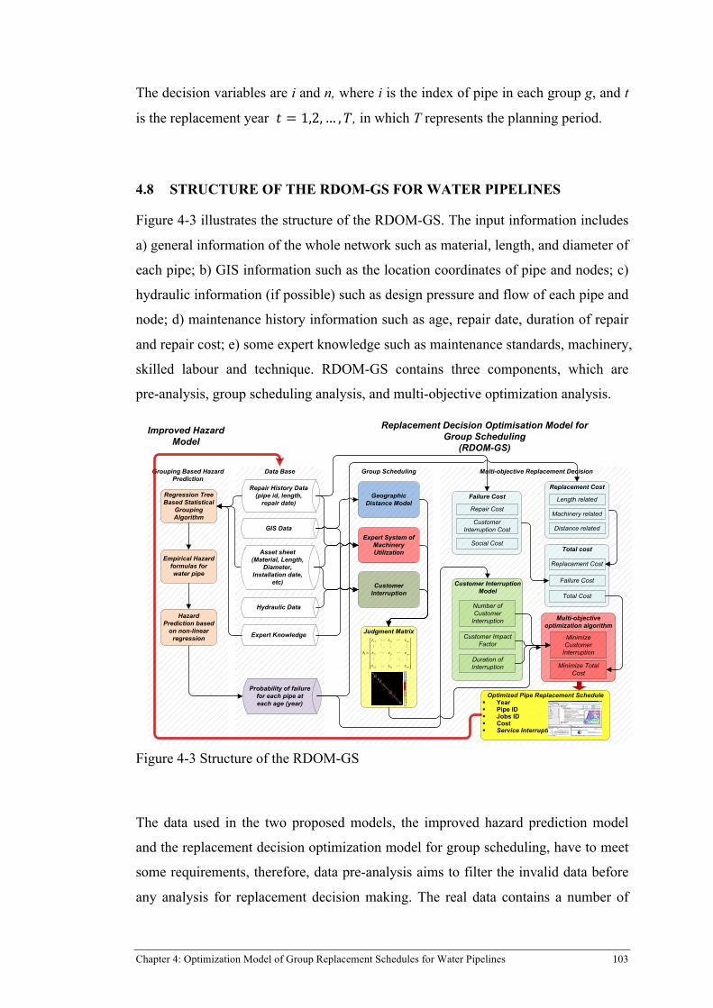
Chapter 4: Optimization Model of Group Replacement Schedules for Water Pipelines 103
The decision variables are i and n, where i is the index of pipe in each group g, and t
is the replacement year 𝑡 = 1,2,… ,𝑇, in which T represents the planning period.
4.8 STRUCTURE OF THE RDOM-GS FOR WATER PIPELINES
Figure 4-3 illustrates the structure of the RDOM-GS. The input information includes
a) general information of the whole network such as material, length, and diameter of
each pipe; b) GIS information such as the location coordinates of pipe and nodes; c)
hydraulic information (if possible) such as design pressure and flow of each pipe and
node; d) maintenance history information such as age, repair date, duration of repair
and repair cost; e) some expert knowledge such as maintenance standards, machinery,
skilled labour and technique. RDOM-GS contains three components, which are
pre-analysis, group scheduling analysis, and multi-objective optimization analysis.
Figure 4-3 Structure of the RDOM-GS
The data used in the two proposed models, the improved hazard prediction model
and the replacement decision optimization model for group scheduling, have to meet
some requirements, therefore, data pre-analysis aims to filter the invalid data before
any analysis for replacement decision making. The real data contains a number of
Multi-objective Replacement Decision
Failure Cost
Customer Interruption Cost
Social Cost
Repair Cost
Replacement Cost
Machinery related
Distance related
Length related
Total cost
Failure Cost
Replacement Cost
Total Cost
Grouping Based Hazard Prediction
Regression Tree Based Statistical
Grouping Algorithm
Empirical Hazard formulas for water pipe
Multi-objective optimization algorithm
Minimize Customer
Interruption
Minimize Total Cost
Customer Interruption Model
Customer Impact Factor
Number of Customer
Interruption
Duration of Interruption
Data Base
Repair History Data(pipe id, length,
repair date)
GIS Data
Asset sheet (Material, Length,
Diameter, Installation date,
etc)
Hydraulic Data
Expert Knowledge
Group Scheduling
Customer Interruption
Expert System of Machinery Utilization
Geographic Distance Model
Judgment Matrix
0.2
0.4
0.6
0.8
1
1.2
1.4
1.6
1.8
2
11 1 1
1
1
j n
i ij in
n nj nn
ε ε ε
ε ε ε
ε ε ε
⎡ ⎤⎢ ⎥⎢ ⎥⎢ ⎥Λ =⎢ ⎥⎢ ⎥⎢ ⎥⎣ ⎦
! !" # " "! !
" " # "! !
Probability of failure for each pipe at each age (year)
Optimized Pipe Replacement Schedule§ Year§ Pipe ID§ Jobs ID§ Cost§ Service Interruption
2010 2015 2020 2025 2030
1.2M
1.4M
1.6M
1.8M
2.0M
2.2M
2.4M
2.6M
2.8M
3.0M Annual Budget Annual Expanse of Non-group Scheduling Mean Value of Non-group Scheduling Annual Expance of Group Scheduling Mean Value of Group Scheduling
Million AU
$ per yea
r
Planning year
Replacement Decision Optimisation Model for Group Scheduling
(RDOM-GS)
Hazard Prediction based
on non-linear regression
Improved Hazard Model
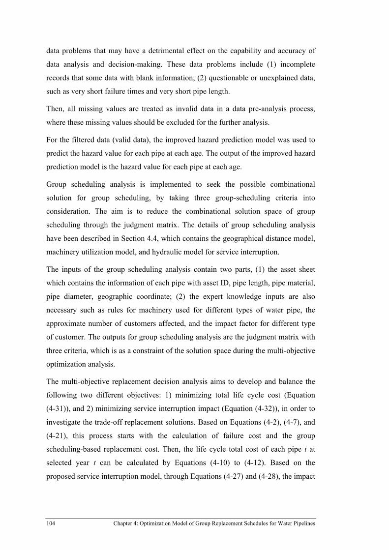
104 Chapter 4: Optimization Model of Group Replacement Schedules for Water Pipelines
data problems that may have a detrimental effect on the capability and accuracy of
data analysis and decision-making. These data problems include (1) incomplete
records that some data with blank information; (2) questionable or unexplained data,
such as very short failure times and very short pipe length.
Then, all missing values are treated as invalid data in a data pre-analysis process,
where these missing values should be excluded for the further analysis.
For the filtered data (valid data), the improved hazard prediction model was used to
predict the hazard value for each pipe at each age. The output of the improved hazard
prediction model is the hazard value for each pipe at each age.
Group scheduling analysis is implemented to seek the possible combinational
solution for group scheduling, by taking three group-scheduling criteria into
consideration. The aim is to reduce the combinational solution space of group
scheduling through the judgment matrix. The details of group scheduling analysis
have been described in Section 4.4, which contains the geographical distance model,
machinery utilization model, and hydraulic model for service interruption.
The inputs of the group scheduling analysis contain two parts, (1) the asset sheet
which contains the information of each pipe with asset ID, pipe length, pipe material,
pipe diameter, geographic coordinate; (2) the expert knowledge inputs are also
necessary such as rules for machinery used for different types of water pipe, the
approximate number of customers affected, and the impact factor for different type
of customer. The outputs for group scheduling analysis are the judgment matrix with
three criteria, which is as a constraint of the solution space during the multi-objective
optimization analysis.
The multi-objective replacement decision analysis aims to develop and balance the
following two different objectives: 1) minimizing total life cycle cost (Equation
(4-31)), and 2) minimizing service interruption impact (Equation (4-32)), in order to
investigate the trade-off replacement solutions. Based on Equations (4-2), (4-7), and
(4-21), this process starts with the calculation of failure cost and the group
scheduling-based replacement cost. Then, the life cycle total cost of each pipe i at
selected year t can be calculated by Equations (4-10) to (4-12). Based on the
proposed service interruption model, through Equations (4-27) and (4-28), the impact
Chapter 4: Optimization Model of Group Replacement Schedules for Water Pipelines 105
of customer interruption for each replacement pipe i at selected year t can be
calculated.
The inputs of the multi-objective replacement decision process contains four parts, (1)
the asset sheet which contains the information of each pipe with asset id, pipe length,
pipe material, pipe diameter, Soil type, installation date, geographic coordinate; (2)
repair notification sheet for all repair history records, which contains the information
of each recorded repair with asset id, pipe length, diameter, material, date of repair,
date of installation; (3) repair cost records with asset id, pipe length, diameter,
material, and repair cost; and (4) expert knowledge of the estimation of replacement
cost. The outputs of the multi-objective replacement decision process are the values
of the two objective functions for each possible group scheduling option.
Then a modified NSGA-II (developed in Chapter 5) as a multi-objective optimisation
algorithm aims to investigate the trade-off solution between the two objectives of
replacement group scheduling. The modified NSGA-II searches the possible group
combinations iteratively with pipe ID, group ID, and replacement year, then
calculates the two objective values and selects the winning combinations, just as the
genes improved in evolution, cross over and mutate to find the optimised solutions.
The inputs are all the inputs in the multi-objective replacement decision analysis, and
the pipe ID group ID and replacement year are coded in the optimisation algorithm.
The outputs are the Pareto front for the two objectives with the total cost and the total
service interruption impact. In the Pareto front, each point contains the information
about which pipes should be due for replacement in each year, and which pipes can
be scheduled as groups, with the information of replacement year, pipe id, group id,
total cost and total service interruption impact during the planning period. This
information will provide the guidance for operators to make replacement decisions.
4.9 SUMMARY
This chapter introduced a multi-objective replacement decision optimisation model
for group scheduling (RDOM-GS) for water pipelines to give planners unambiguous
information for optimizing their water pipeline replacement planning. Two objective
functions were developed, based on cost functions and service interruption function.
This model allowed planners to develop group replacement schedules against three
criteria: shortest geographic distance, maximum replacement equipment utilization,

106 Chapter 4: Optimization Model of Group Replacement Schedules for Water Pipelines
and minimum service interruption, which were modelled by the Judgment matrix.
The RDOM-GS integrated cost analysis, service interruption analysis, and
optimization analysis, to deliver schedules that limit service interruptions and
minimize total life-cycle cost.
Replacement group scheduling optimisation problem (GSOP) is considered as one of
the multi-objective combinatorial optimisation, but it is different from any of the
classic combinatorial optimisation problems. A modified evolutionary optimisation
algorithm is developed and introduced in Chapter 5 to deal with the proposed
multi-objective replacement decision optimisation for water pipelines.
Chapter 5: An Improved Multi-objective Optimisation Algorithm for Group Scheduling 107
Chapter 5: An Improved Multi-objective Optimisation Algorithm for Group Scheduling
5.1 INTRODUCTION
Group scheduling for water pipeline replacement optimisation is complex, because it
contains multiple criteria, multiple objectives, and its decision variables are in both
time and space domains. However, the description of this problem can hardly be
found in the literature. Therefore a mathematical modelling of the group scheduling
optimisation problem (GSOP) and its computational complexity are discussed in
Section 5.2. A modified NSGA-II to deal with GSOP is developed, and its procedure
is introduced in Section 5.3, followed by the modified NSGA-II operators in Section
5.4. A comparison study for the modified NSGA-II and original NSGA-II based on
two simplified objective functions is conducted in Section 5.5.
5.2 GROUP SCHEDULING OPTIMISATION PROBLEM (GSOP)
Optimisation problems can be divided into two categories: those with continuous
variables and those with discrete variables, which are called the combinatorial
problems [123]. Combinatorial optimization problems are characterized by their
well-structured problem definition as well as by their huge number of solution spaces
in practical application areas. Especially in areas like routing, task allocation, or
scheduling, such kinds of problems often occur [124].
A multi-objective optimisation problem with m objectives and n parameters is
usually described as a nonlinear programming problem, which is given as:
minimize: 𝑓! 𝑋 , 𝑋 = 𝑥!, 𝑥!,… , 𝑥! ,𝑋 ∈ 𝑆
subject to: 𝑔! 𝑋 = 0, 𝑖 = 1,2,… ,𝑝
𝑘! 𝑋 ≥ 0, 𝑗 = 1,2,… , 𝑞,
where 𝑓! 𝑋 indicates the m objective functions, and 𝑔! 𝑋 and 𝑘! 𝑋 indicate
the constrains.

108 Chapter 5: An Improved Multi-objective Optimisation Algorithm for Group Scheduling
The group scheduling optimisation problem (GSOP) can be considered as one of the
multi-objective combinatorial optimisation, which is addressed as below:
Given a water pipelines network with n individual pipes, with index of i, i = 1,2,…,n,
𝑁𝑂𝑃! is defined as the number of pipes in each group 𝑔, where 𝑔 is the index of
each group, 𝑔 = 1, 2,…, NOG. NOG is the total number of groups in the whole water
pipelines network. Given a replacement planning horizon of T years, and given a
maximum number of pipes in each group 𝑁𝑂𝑃∗ , 𝑁𝑂𝑃∗ = max(𝑁𝑂𝑃!) , the
objective of GSOP is to find the best group index 𝑔, and the best year 𝑡, 𝑡 =
1,2,… ,𝑇, for each pipe i, in order to minimise the total system cost (Equation (4-31)),
and to minimise the total system impact of service interruption(Equation (4-32)).
Two infinite situations are considered: (1) for all group 𝑔, 𝑁𝑂𝑃! equals to 1, which
means that there is no pipe combined together, then NOG = n; (2) for all group 𝑔,
𝑁𝑂𝑃! = 𝑁𝑂𝑃∗, which means that combined pipes in each group reach the maximum
number 𝑁𝑂𝑃∗, then the NOG = n/𝑁𝑂𝑃∗, where it has:
!!"#∗
≤ 𝑁𝑂𝐺 ≤ 𝑛.
Therefore, using the judgment value, 𝑥!" , defined in Equation (4-21), 𝑁𝑂𝑃! is
given as:
𝑁𝑂𝑃! = 𝑥!"!!!! . (5-1)
Based on that, there exists
𝑥!"!!!!
!!!! = 𝑛, (5-2)
where the sum of all pipes in all groups is equal to the total number of pipes.
The possible numbers of the combinational solutions have an exponential
relationship with the total number of pipes. There will be 𝑁𝑂𝐺^𝑁 ∗ 𝑇^𝑁 numbers
of combinational options, if there are the number of N pipes and NOG number of
replacement activity groups, and the planning period is T years, where “^” means the
power operator. Normally, one water pipeline network contains at least thousands of
pipes, and the replacement-planning period is usually more than 20 years, thus,
Chapter 5: An Improved Multi-objective Optimisation Algorithm for Group Scheduling 109
searching from the corresponding huge solution space of the combinational options
occupies huge computational memory.
A number of classical mathematical programming-based techniques such as the
Newton method, linear programing, dynamic programming, nonlinear programming,
had been developed to handle the combinatorial optimization problem [123].
However, GSOP is a complex combinatorial optimization problem involving
multiple nonlinear objective functions, nonlinear constraints, and discrete variables.
Therefore, in practice, heuristics such as evolutionary optimization technologies are
commonly used even if they are unable to guarantee an optimal solution.
According to the literature review in Chapter 2, a number of contributions on
evolutionary optimization algorithms had previously been developed. Since the
multi-objective GSOP is hardly found at all in the literature, a well-known
evolutionary optimization algorithm, Non-dominated sorting genetic algorithm-II
(NSGA-II) is modified in order to solve the multi-objective GSOP. Several NSGA-II
operators are redesigned or modified, and the details will be described in the
following sections.
5.3 PROCEDURE OF THE MODIFIED NSGA-II
In this research, the modified NSGA-II contains a number of operators. Some of
them are redesigned or modified for better performance. These include: a new
designed coding method, an initialization method, a multi-point crossover operator, a
modified non-dominated sorted mutation operator (considering keeping pipe in the
same group replaced at the same year), non-dominated sort operator, a modified
crowding distance operator, and a modified rank based selection operator.
The overall structure of the modified NSGA-II is illustrated in Figure 5-1. From the
beginning, a set of initial population is generated based on the new coding and
initialisation methods, indicated as Pgen, where gen means generation, and equals “0”
in this step. Then, the population Pgen is sorted with respect to its Pareto rank. By
new individuals competed with the parent population Pgen, temporary population Qgen
is achieved with the selection, crossover, and mutation operator. By combining the
Pgen and Qgen, Rgen is created. Then Rgen is sorted by non-dominated sorting to produce
a series of non-dominated set Ft ={F1, F2, ..., Fm}. Due to F1 including the best

110 Chapter 5: An Improved Multi-objective Optimisation Algorithm for Group Scheduling
individuals of Rgen, F1 is added into the new parent population Pgen+1. If the size of F1
less than Pop (number of individuals), then continue to add F2 to Pgen+1, until add F3.
If the size of the population is beyond Pop, the individuals in F3 are based on the
crowding distance operation to reduce population size to Pop. Then repeat the circle
again, until the number of generation is equal to the maximum generation. The
outputs are a Pareto-set of solutions with the individuals with the information of
group number g and the replacement year t, followed by the values of the two
objective functions.
The procedure is shown in Figure 5-1. In the next section, the details of each operator
will be introduced.
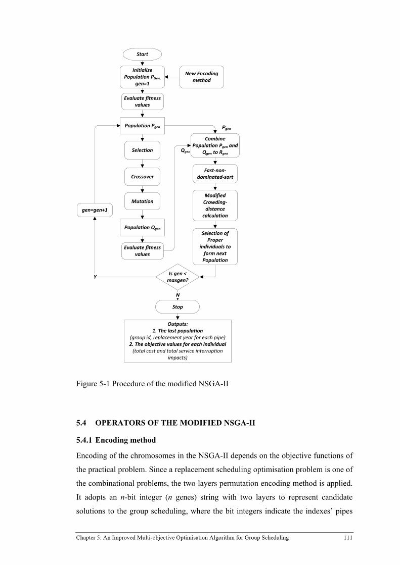
Chapter 5: An Improved Multi-objective Optimisation Algorithm for Group Scheduling 111
Figure 5-1 Procedure of the modified NSGA-II
5.4 OPERATORS OF THE MODIFIED NSGA-II
5.4.1 Encoding method
Encoding of the chromosomes in the NSGA-II depends on the objective functions of
the practical problem. Since a replacement scheduling optimisation problem is one of
the combinational problems, the two layers permutation encoding method is applied.
It adopts an n-bit integer (n genes) string with two layers to represent candidate
solutions to the group scheduling, where the bit integers indicate the indexes’ pipes
Start
Initialize Population PGen,
gen=1
Combine Population Pgen and
Qgen to Rgen
gen=gen+1
Y
Population Qgen
Crossover
Mutation
Selection
Pgen
Qgen
Is gen < maxgen?
Stop
Fast-‐non-‐dominated-‐sort
Modified Crowding-‐distance
calculation
Selection of Proper
individuals to form next Population
N
Population Pgen
Evaluate fitness values
Evaluate fitness values
Outputs:1. The last population
(group id, replacement year for each pipe)2. The objective values for each individual(total cost and total service interruption
impacts)
New Encoding method
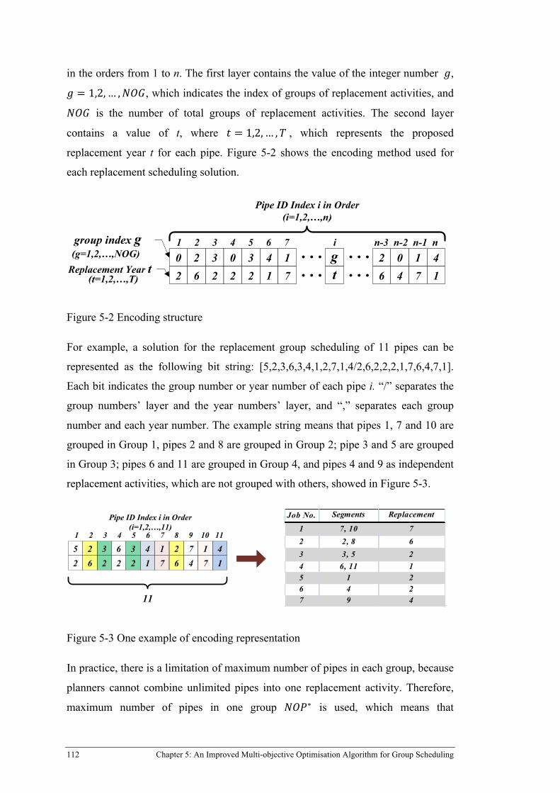
112 Chapter 5: An Improved Multi-objective Optimisation Algorithm for Group Scheduling
in the orders from 1 to n. The first layer contains the value of the integer number 𝑔,
𝑔 = 1,2,… ,𝑁𝑂𝐺, which indicates the index of groups of replacement activities, and
𝑁𝑂𝐺 is the number of total groups of replacement activities. The second layer
contains a value of t, where 𝑡 = 1,2,… ,𝑇 , which represents the proposed
replacement year t for each pipe. Figure 5-2 shows the encoding method used for
each replacement scheduling solution.
Figure 5-2 Encoding structure
For example, a solution for the replacement group scheduling of 11 pipes can be
represented as the following bit string: [5,2,3,6,3,4,1,2,7,1,4/2,6,2,2,2,1,7,6,4,7,1].
Each bit indicates the group number or year number of each pipe i. “/” separates the
group numbers’ layer and the year numbers’ layer, and “,” separates each group
number and each year number. The example string means that pipes 1, 7 and 10 are
grouped in Group 1, pipes 2 and 8 are grouped in Group 2; pipe 3 and 5 are grouped
in Group 3; pipes 6 and 11 are grouped in Group 4, and pipes 4 and 9 as independent
replacement activities, which are not grouped with others, showed in Figure 5-3.
Figure 5-3 One example of encoding representation
In practice, there is a limitation of maximum number of pipes in each group, because
planners cannot combine unlimited pipes into one replacement activity. Therefore,
maximum number of pipes in one group 𝑁𝑂𝑃∗ is used, which means that
2 3 3 40 0 1g6 2 2 12 4t 7
02
17
26
41
Pipe ID Index i in Order(i=1,2,…,n)
group index g
Replacement Year t
1 2 3 4 5 6 7 i n-3 n-2 n-1 n (g=1,2,…,NOG)
(t=1,2,…,T)
11
Job No. Segments Index
Replacement Year1 7, 10 7
2 2, 8 63 3, 5 24 6, 11 15 1 26 4 27 9 4
2 3 3 456 2 2 12
62
17
7 14 7
26
41
1 2 3 4 5 6 7 8 9 10 11
Pipe ID Index i in Order(i=1,2,…,11)
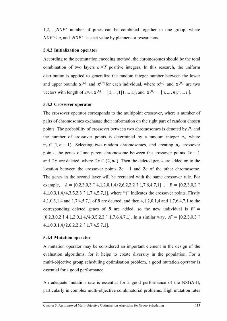
Chapter 5: An Improved Multi-objective Optimisation Algorithm for Group Scheduling 113
1,2,…,𝑁𝑂𝑃∗ number of pipes can be combined together in one group, where
𝑁𝑂𝑃∗< n, and 𝑁𝑂𝑃∗ is a set value by planners or researchers.
5.4.2 Initialization operator
According to the permutation encoding method, the chromosomes should be the total
combination of two layers n×T positive integers. In this research, the uniform
distribution is applied to generalize the random integer number between the lower
and upper bounds 𝐱(!) and 𝐱(!)for each individual, where 𝐱(!) and 𝐱(!) are two
vectors with length of 2×n,𝐱(!) = 1,… ,1|1,… ,1 , and 𝐱(!) = 𝑛,… ,𝑛|𝑇,…𝑇 .
5.4.3 Crossover operator
The crossover operator corresponds to the multipoint crossover, where a number of
pairs of chromosomes exchange their information on the right part of random chosen
points. The probability of crossover between two chromosomes is denoted by Pc and
the number of crossover points is determined by a random integer nc, where
𝑛! ∈ [1,𝑛 − 1). Selecting two random chromosomes, and creating 𝑛! crossover
points, the genes of one parent chromosome between the crossover points 2𝑐 − 1
and 2𝑐 are deleted, where 2𝑐 ∈ (2,𝑛𝑐). Then the deleted genes are added on to the
location between the crossover points 2𝑐 − 1 and 2𝑐 of the other chromosome.
The genes in the second layer will be recreated with the same crossover rule. For
example, 𝐴 = [0,2,3,0,3 ↑ 4,1,2,0,1,4/2,6,2,2,2 ↑ 1,7,6,4,7,1] , 𝐵 = [0,2,3,0,2 ↑
4,1,0,3,1,4/4,3,5,2,3 ↑ 1,7,4,5,7,1], where “↑” indicates the crossover points. Firstly
4,1,0,3,1,4 and 1,7,4,5,7,1 of B are deleted, and then 4,1,2,0,1,4 and 1,7,6,4,7,1 to the
corresponding deleted genes of B are added, so the new individual is 𝐵” =
[0,2,3,0,2 ↑ 4,1,2,0,1,4/4,3,5,2,3 ↑ 1,7,6,4,7,1]. In a similar way, 𝐴” = [0,2,3,0,3 ↑
4,1,0,3,1,4/2,6,2,2,2 ↑ 1,7,4,5,7,1].
5.4.4 Mutation operator
A mutation operator may be considered an important element in the design of the
evaluation algorithms, for it helps to create diversity in the population. For a
multi-objective group scheduling optimisation problem, a good mutation operator is
essential for a good performance.
An adequate mutation rate is essential for a good performance of the NSGA-II,
particularly in complex multi-objective combinatorial problems. High mutation rates

114 Chapter 5: An Improved Multi-objective Optimisation Algorithm for Group Scheduling
lead to a random search throughout the search space, while low mutation rates
present very small rates of progress towards the Pareto front, leading to time
consuming and ineffective procedures.
In general, a fix value for the mutation probability may be adequate in the initial
phase of the search but may become very ineffective, when the population is near the
Pareto front. Moreover, another rule for mutation is that the worse the value of the
objective function, the greater the mutation probability and vice versa [125].
Therefore, to improve the mutation operator for a group scheduling optimisation
problem, the dynamic mutation operator based on the non-dominated fitness is
introduced, where it has considered the influence of the mutation probability from
the non-dominated fitness values.
The new established non-dominated fitness based Gaussian mutation operator is
given as:
𝐱(!!!) = 𝐱(!) + 𝑃!,!(!) ∙ 𝐱(!) − 𝐱(!) ∙ 𝜹, (5-3)
where 𝐱𝒋(!) indicates each individual j, j=1,…Pop, Pop indicates the population size,
and 𝐱𝒋(!) = (𝑥!,!! ,… , 𝑥!,!
(!)) belongs to the tth generation. 𝐱(!) and 𝐱(!) are the upper
and lower bounds vectors for each 𝑥!,!! , 𝑘 = 1,… ,𝑛. 𝜹 is a vector of normally
distributed random numbers, 𝑁(1,𝜎!), where the mean is 0, and the standard
deviation is 𝜎!. 𝑃!,!(!) is the mutation probability for individual j at tth generation,
which is given as:
𝑃!,!(!) = 𝜎! ∙ 1− 𝜌 ∙
!!"# !
∙ 𝑓𝑖𝑡𝑛𝑒𝑠𝑠! , (5-4)
where t represents current evolution generation, max t indicates the largest evolution
generation, and 𝑓𝑖𝑡𝑛𝑒𝑠𝑠! represents the non-dominated fitness value for individual j.
Parameter 𝜌 is in the scalar between 0 and 1, 𝜌 ∈ [0,1].
At the beginning generation, the individuals are at a far distance from the Pareto
front, therefore, large probability can maintain the diversity of the population, and
the greater probability can deal with the non-good individuals (whose non-dominated
fitness values are higher than others). In the end generation, the whole population has

Chapter 5: An Improved Multi-objective Optimisation Algorithm for Group Scheduling 115
been basically close to the front, mutation rate decreases, therefore, it prevents the
population degenerating earlier.
For optimisation of group replacement schedules, pipes combined in one group g
should be replaced at the same year t. However, this cannot be guaranteed by the
permutation encoding of the second layer. For example, in Figure 5-3, for pipe 2 and
pipe 8, they are both grouped in group 2, but, initially, 𝑡! and 𝑡! may not be equal,
where 𝑡! indicates the replacement year for pipe i, and i = [1,n]. Therefore, a
reformation step is introduced in the mutation operator to keep the year t correct for
each pipe i in each group g.
The reformation step is defined to keep 𝑡! identical in each group g, which is given
as:
𝑡!∗ =!!∙!!"
!!!!
!!"!!!!
, (5-5)
where 𝑡!∗ is the new replacement year t for each pipe in group 𝑔, and 𝑥!" is a
judgment value introduced in Equation (4-21). The reformation step is shown as
below:
Reformation step of mutation Set 𝑖, 𝑗, 𝑘 , 𝑘 = 1,… ,𝑃𝑜𝑝, 𝑖 = 1,… , 𝑛, 𝑗,𝑔 = 1,… ,𝑁𝑂𝐺
k is the index of individuals, i is the index of gene(pipe), j is the index of group number 𝑔
for each individual k, for each group number 𝑔
find all the index i, where 𝑗 = 𝑔
for all the index i, find all 𝑡! 𝑡! is the replacement year value of each gene i Let 𝑡!∗ =
!"# !" !"" !!! !!!"#$%& !" !"" !!! !!
New 𝑡! = 𝑡!∗
5.4.5 Crowding distance operator
Crowding distance for a member of a non-dominated set tries to approximate the perimeter of a cuboid formed using the nearest neighbors of the member, which can easily handle the Case 1 problem showed in Figure 5-4. However, a main problem of
crowding distance has been illustrated in Figure 5-4 that, individual i and i+1 are located very close to each other in the left figure (Case 2), but they are far from the other individuals.

116 Chapter 5: An Improved Multi-objective Optimisation Algorithm for Group Scheduling
Figure 5-4 Illustration of the original crowding distance method
In Case 2, the values of individual i and i+1 may be quite close, and both of them will be removed or reserved in crowding distance measurement. Obviously, it doesn’t benefit the distribution of the non-dominated set. A better solution would be keeping one of the individuals, either individual i or i+1 and removing the other individual. A minimum spanning tree [85] is used to deal with this problem. However, this method has a drawback in that it must calculate the minimum spinning tree every time, and it seems unclear for a solution if one node has two more edges connected. Based on these concerns, a simple modified crowding distance is proposed in this research to handle both situations in Case 1 and Case 2.
Based on the definition of crowding distance[83], the crowding distance for solution i is given as:
𝐼[𝑖]!"#$%&'( = 𝐼[𝑖]!"#$%&'( +! !!! .!!! !!! .!
!!!"#!!!!"# . (5-6)
and the modified crowding distance is given as:
𝐼 𝑖 !"#$%&'( = 𝐼 𝑖 !"#$%&'(
+ ! !!! .!!! !!! .!!!!"#!!!!"# ∙ 1+ !"# ! !!! .!!! ! .! , ! ! .!!! !!! .!
!"# ! !!! .!!! ! .! , ! ! .!!! !!! .!, (5-7)
where ! !!! .!!! ! .!! ! .!!! !!! .!
indicates the crowding deviation of i between solution i-1 and
i+1, which is shown in Figure 5-5.
f1
f2
I(i-1)
i
i+1
I(i+1)
i-1 I(i)
f1
f2
I(i)
i
i+1I(i+1)
Case 1 Case 2

Chapter 5: An Improved Multi-objective Optimisation Algorithm for Group Scheduling 117
Figure 5-5 Modified crowding distance
Therefore, the procedure of the modified crowding distance is as below:
Modified-crowding-distance-assignment (I) 𝑙 = |𝐼| number of solutions in I
for each i, set 𝐼[𝑖]!"#$%&'( = 0 initialize distance for each objective m
𝐼 = 𝑠𝑜𝑟𝑡(𝐼,𝑚)
if i = 1 or i = l:
Sorting based on each objective value,
𝐼[1]!"#$%&'( = 𝐼[𝑙]!"#$%&'( = ∞ so that boundary points are always selected
otherwise: for i = 2 to (l-1)
for all other points
𝐼[𝑖]!"#$%&'( = 𝐼[𝑖]!"#$%&'( +𝐼 𝑖 + 1 .𝑚 − 𝐼 𝑖 − 1 .𝑚
𝑓!!"# − 𝑓!!"#∙𝐼 𝑖 + 1 .𝑚 − 𝐼 𝑖 .𝑚𝐼 𝑖 .𝑚 − 𝐼 𝑖 − 1 .𝑚
5.4.6 Selection Operator
The selection operator aims to ensure that better members of individuals in the
current generation can be selected with higher probability of reproducing offspring in
the hopes of acquiring higher fitness values in the next generation. At the same time,
to ensure finding the global optimum, and to avoid converging to local optimum, the
worse members of population have a smaller probability of being selected. Three
often-used selection operators are tournament selection, roulette wheel selection and
rank-based roulette wheel selection. The rank-based roulette wheel selection with its
advantages of avoiding premature convergence and eliminating the need to scale
f1
f2I(i).m1 i
i+1
i-1
I(i+1).m1
I(i-1).m1
ii-1 i+1
! ! + 1 .! − ! ! − 1 .!
! ! + 1 .! − ! ! .!
! ! .! − ! ! − 1 .!
118 Chapter 5: An Improved Multi-objective Optimisation Algorithm for Group Scheduling
fitness values is used in this research. The probability of an individual being selected
is based on its fitness rank:
𝑅𝑎𝑛𝑘 𝑃𝑜𝑠 = 2− 𝑆𝑃 + 2 ∙ 𝑆𝑃 − 1 ∙ !"#!!!!!
, (5-8)
where SP is the selective pressure, 𝑆𝑃 ∈ [1,2], Pos indicates the position of an
individual in the sorted population, where 𝑃𝑜𝑠 = 1,… ,𝑃𝑜𝑝, Pop is the population
size.
5.5 COMPARATIVE STUDY
In order to test the proposed modified NSGA-II for GSOP, and to compare its
performance with the original NSGA-II, the modified NSGA-II is used to solution a
simplified GSOP. Commercial software Matlab R2012a is used to program the
optimisation algorithms.
5.5.1 Simplified objective functions
Since the actual objective functions Equation(4-31) and Equation(4-32) are very
complex, two simplified objective functions are designed for testing the performance
of the modified NSGA-II for GSOP.
In Equation(4-7), the failure probability for each pipe i at each year t was assumed to
be a constant value 𝑓!"#=0.001. Repair cost equals to $500/unit, replacement cost
assume to be $500/meter.
Equation(4-28) is simplified as that 𝐼𝑐!"#$,! follows a normal distribution with mean
equal to the diameter of pipe i, and the standard deviation assumed to be 1/4 of mean.
It is reasonable that the larger diameter pipe has higher water flow, which supplies
water to more customers.
One hundred pipes were randomly selected from a water pipe data set introduced in
Section 3.3.2.
5.5.2 Parameter settings
NSGA-II and the modified NSGA-II are given integer-valued decision variables. The
population size, pop, is 100, the maximum generation equals 100. One hundred pipes
are considered (n = 100), therefore, there are 100 design variables. Maximum
number of pipes in each group is equal to 5, therefore the lower and upper bounds

Chapter 5: An Improved Multi-objective Optimisation Algorithm for Group Scheduling 119
are 𝐱(!) = 1,… ,1 , and 𝐱(!) = 100,… ,100 . The number of objective function is
2.
A crossover probability of pc = 0.8 and in the mutation operator, the standard
deviation 𝜎! = 2, 𝜌 = 0.3 . In the selection operator, the selective pressure,
𝑆𝑃 = 1.1.
5.5.3 Results comparison
The multi-objective optimization has two goals to measure its performance, the
convergence to the Pareto-optimal set and the maintenance of diversity in the
solutions of the Pareto-optimal set.
Figure 5-6 shows the Pareto-fronts of the optimisation results for two optimisation
methods. The blue solid square and the red dot indicate the Pareto-fronts calculated
by NSGA-II and the modified NSGA-II respectively. During the same generation
(gen = 100), the modified NSGA-II got better results, where its Pareto-front has a
lower position compared with the NSGA-II one, which shows that the modified
NSGA-II has better optimisation results in the same generation, for getting
replacement schedules subject to lower total cost and lower service interruption.

120 Chapter 5: An Improved Multi-objective Optimisation Algorithm for Group Scheduling
Figure 5-6 Pareto-fronts of the optimisation results for NSGA-II and the modified NSGA-II
To measure the diversity in the solutions of the Pareto-optimal set, 𝜟 metric was
introduced [83], where a set of good solutions is necessary to be spanned over the
entire Pareto-optimal region, and the Δ is to measure how the solutions are spanned,
see equation below,
Δ = !!!!!! |!!!!|!!!!!!
!!!!!!(!!!)!, (5-9)
where 𝑑! is the Euclidean distance between consecutive solutions in the obtained
non-dominated set of solutions, 𝑑 is the average value of 𝑑!, 𝑑! and 𝑑! are the
Euclidean distances between the extreme solutions and the boundary solutions of the
obtained non-dominated set, and N is the total number of the solutions.
Δ! for NSGA-II equals to 1.16, and Δ! for the modified NSGA-II equals to 1.07,
where Δ! > Δ!. The smaller the Δ is, the better the distribution of the solution is,
6.0E+04
8.0E+04
1.0E+05
1.2E+05
1.4E+05
1.6E+05
1.8E+05
9.1E+06 9.2E+06 9.3E+06 9.4E+06 9.5E+06 9.6E+06 9.7E+06 9.8E+06
Objective 1
Objective 2
NSGA-‐II
Modi6ied NSGAII
Chapter 5: An Improved Multi-objective Optimisation Algorithm for Group Scheduling 121
therefore, the modified NSGA-II has made a better diversity in the solutions of the
Pareto-optimal set than the NSGA-II.
5.6 SUMMARY
In this chapter, the candidate firstly described the group scheduling optimisation
problem (GSOP) and its computational complexity, followed by the development of
a modified NSGA-II to deal with the GSOP, which includes the introduction of the
procedure and the operators for the modified NSGA-II. Finally, a comparison study
was conducted based on the original NSGA-II and modified NSGA-II. The results
showed that the modified NSGA-II has a better convergence to the Pareto-optimal
set and results in better diversity in the solutions of the Pareto-optimal set.
A case study for a water utility is described in Chapter 6 to show the application of
the improved hazard model (Chapter 3) and the RDOM-GS (Chapter 4 and Chapter
5).

Chapter 6: A Case Study 123
Chapter 6: A Case Study
6.1 INTRODUCTION
This chapter introduces a real case study from a water utility in Queensland to test
and validate the proposed two models, (1) the improved hazard model for water
pipes, and (2) the RDOM-GS. This water utility is one of the participants of the
Cooperative Research Centre for Infrastructure and Engineering Asset Management
(CIEAM), and provides water and wastewater services to more than 850,000
consumers. To support the study, the water utility provided a number of sets of data,
including pipeline network data and work order data (in Excel spread sheets) and
GIS data (in MapInfo files), described as follows:
Pipeline network data indicates the general information of the water pipes, which has
71,571 sets of raw data with the information of pipe ID (an unique identification for
each pipe), pipe length (metres), pipe material types, pipe diameters (millimetres),
construction date, and sub area ID (an identification for particular area defined by the
water utility).
Work order data is the repair history data, which has 6,459 sets of raw data with
information of pipe ID (a unique identification for each pipe), repair work order ID
(an unique identification for each repair activity), repair start date, repair end date,
activity description (to describe the activity in details), street name (where the pipe is
located), and suburb name (where the pipe is located).
GIS data includes all the geographical information in MapInfo files for the water
network, which includes geographic coordinates of water pipes, nodes, valves, pump
stations and reservoirs.
The three files, the pipeline network data file, the work order data file, and GIS data
files, can be linked by the pipe ID, so that all general information such as pipe length,
diameter, material, location can be shared within the three files.
This case study includes a three-steps process: (1) data pre-analysis to investigate the
provided data, to exclude invalid data, and to analyse the general characteristics; (2)

124 Chapter 6: A Case Study
statistical-based hazard prediction analysis using the proposed improved hazard
model, which has partitioned data into different subgroup based on their
homogeneity, calculate empirical hazard for each subgroup, generate fitted hazard
curve for failure prediction; (3) replacement decision optimisation for group
scheduling using the proposed RDOM-GS, which gives an optimised replacement
planning taking total cost and customer interruption into consideration, followed by a
comparison analysis to show how well the replacement planning is working,
compared with the method that does not consider the group scheduling.
6.2 DATA PRE-ANALYSIS
6.2.1 Overview of the water pipeline network
This water pipeline network services a community in Queensland, Australia, and
comprises 66,405 pipes (total length of 3,640km, at an average length of pipe of
54.79m), with diameters from 20mm to 1440mm, in 11 different materials, installed
between 1937 and 2012. It services a population of more than 850,000 inhabitants.
Based on the pipeline network data file, an overview of the network was presented in
Table 6-1.
Table 6-1 Overview of the water pipeline network
Item Description Pipe’s Diameter
20mm, 32mm, 40mm, 45mm, 50mm, 63mm, 75mm, 80mm, 90mm, 100mm, 110mm, 150mm, 200mm, 220mm, 250mm, 300mm, 375mm, 411mm, 450mm, 500mm, 510mm, 525mm, 565mm, 590mm, 600mm, 660mm, 700mm, 750mm, 800mm, 850mm, 900mm, 915mm, 960mm, 965mm, 1050mm, 1125mm, 1290mm, 1440mm
Pipe’s Material (11 types)
Asbestos Cement(AC), Cast Iron Cement Lined(CICL), Concrete(CONC), Copper(CU), Fibre Reinforced Pipe(FRR), Galvanised Steel(GAL), Glass Reinforced Plastic(GRP), Glass Reinforced Plastic(HOBAS), Ductile Iron Cement Lined(DICL), Mild Steel Concrete Lined(MSCL), Unplasticised Poly Vinyl Chloride(UPVC)
Pipe’s Length
From 0.1m to 1363.9m
Zone area types
RURAL (RUR), URBAN (URB), HIGH DENSITY URBAN (HDU), CBD
Population More than 850,000 inhabitants
6.2.2 Age Profile of the Water Pipeline Network
The oldest water pipes in the network date back to 1937. Around 102km of the total
length of pipes now in operation were installed before 1960. The construction history
and the cumulative length of pipe being installed for each calendar year are shown in
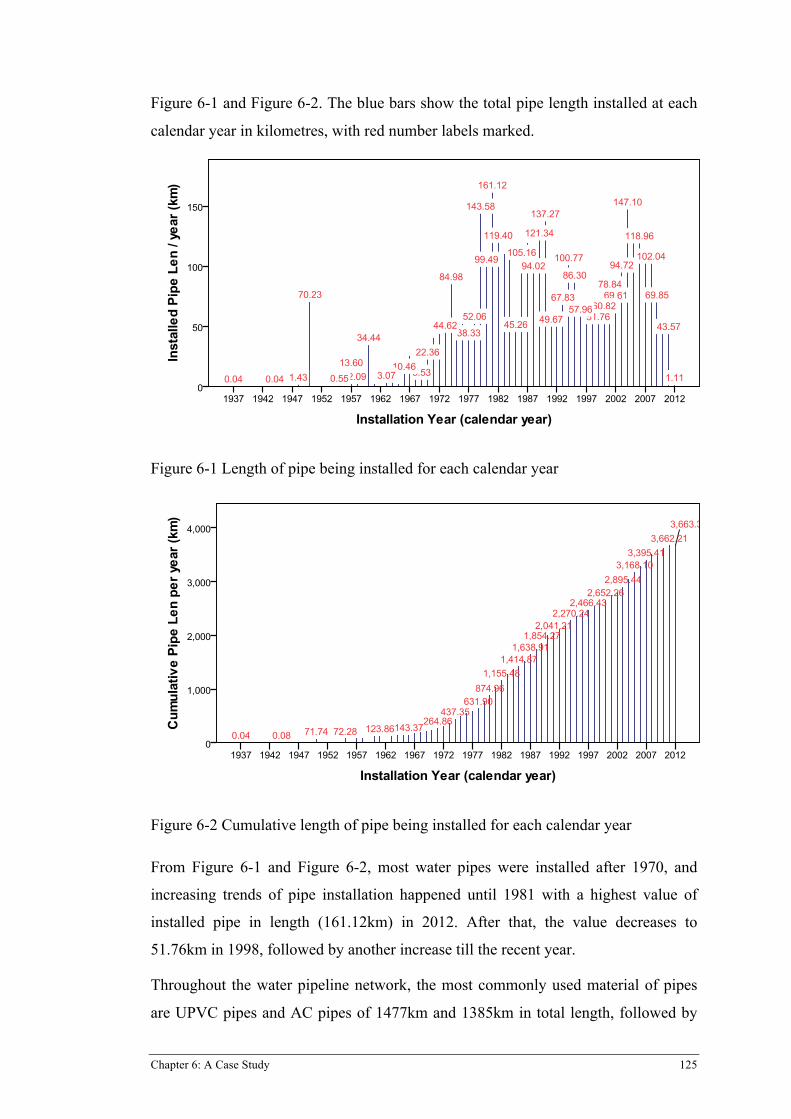
Chapter 6: A Case Study 125
Figure 6-1 and Figure 6-2. The blue bars show the total pipe length installed at each
calendar year in kilometres, with red number labels marked.
Figure 6-1 Length of pipe being installed for each calendar year
Figure 6-2 Cumulative length of pipe being installed for each calendar year From Figure 6-1 and Figure 6-2, most water pipes were installed after 1970, and
increasing trends of pipe installation happened until 1981 with a highest value of
installed pipe in length (161.12km) in 2012. After that, the value decreases to
51.76km in 1998, followed by another increase till the recent year.
Throughout the water pipeline network, the most commonly used material of pipes
are UPVC pipes and AC pipes of 1477km and 1385km in total length, followed by

126 Chapter 6: A Case Study
DICL, MICL, and CICL. Other material includes CU, FRR, GAL, GRP, and pipes
marked as NOINF, which means the pipes lacking material information. Figure 6-3
shows the total length of pipe with different material types.
Figure 6-3 Total length of pipe by material type
Figure 6-4 compares the six material types for diameters, which shows that material
type has a significant relationship with diameter. Most UPVC and AC pipes have
small diameters around 150mm; DICL and CICL has larger range of diameters;
MSCL pipe has largest average diameter of around 700mm, where, in general, most
of the water mains with diameter larger than 500mm are MSCL pipes.

Chapter 6: A Case Study 127
Figure 6-4 Box plot for different material types of diameter
Figure 6-5 compared six material types for the installation date. Almost all concrete
or cement pipes were installed before 1960. During the years from 1961 to 1990, a
significant increase of water pipe installations can be seen. Nearly half the numbers
of the total pipes (3/5 of total length) were constructed in this period. The most
commonly used materials in that period were ductile iron, grey cast iron and mild
steel. In 1960, the first PVC pipes were installed and have become the preferred pipe
material for replacements and expansions after 1970s. CICL pipes were constructed
in the early years around 1950 and most of them were alternated by DICL in recent
years.

128 Chapter 6: A Case Study
Figure 6-5 Box plot for different material types of installation date
6.2.3 Repair history of water pipe
The observation period over which the repair history records were collected and kept
is just more than 10 complete years from 2002 to 2012. The water company
conducted 6,459 repair jobs for unexpected breaks. Some of these data were found to
be missing for various reasons, only 4,635 sets of valid records are with complete
information of ID, length, material, diameter, installed date, repair date and repair
cost, which includes 2,926 pipes, which indicates that a number of pipes were
repaired two or more times. Over 10 years, the water utility spent around AUD$4
million to repair the water pipes. Figure 6-6 shows that the repair cost correlated with
the number of breaks, where the repair cost rose from 2000 to 2010, and decreased
slightly in 2005, and then peaked at AU$0.86 million in 2010.

Chapter 6: A Case Study 129
Figure 6-6 Repair history from 2000 to 2010
The repair records corresponded to six different pipe materials. Figure 6-7 showed
the number of failures by material type, and that AC pipe has the highest number of
failures (1,458), followed by UPVC (574). CICL, DICL and MSCL had 123, 80 and
23 failures respectively. Other pipe materials had a total of 16 failures during the
10-year observation period.
Figure 6-7 Number of breaks by material types In practice, water pipe should be treated as a combination of a number of pipe
segments. Repair activities are only for pipe segments rather than the whole water
pipe, which is introduced in Chapter 4. Therefore, to illustrate the situation of water
2000 2002 2004 2006 2008 2010
100k
200k
300k
400k
500k
600k
700k
800k
900k
150
200
250
300
350
400
450
500
Num
ber o
f bre
aks a
t yea
r rou
nd
Rep
air c
ost a
t yea
r rou
nd (A
U$)
Calendar year
Repair cost Number of breaks

130 Chapter 6: A Case Study
pipe failures in the network, the number of breaks pre 100km by material types are
introduced and shown in Figure 6-8. Most failures happened in AC pipes at its early
installed date. CICL has more failures pre 100km than DICL, which explains the
reason of the substitution of DICL with CICL.
Figure 6-8 Number of breaks per 100km by material types
Table 6-2 is a summary of pipes based on types of material. It illustrates that the
water network consists mainly of AC (29.6%), DICL (20.3%), and UPVC (42.0%)
pipes. From the failure record point of view, AC and UPVC take 66.3% and 25.2%
of the total failure records, which means 10% of AC pipes and 1.02% of UPVC pipes
had failure records from 2000 to 2012.
Table 6-2 Summary of pipes based on types of material
Material No. of pipes
% of total pipes
No. of failures
% of total failures
No. of failures/ No. of pipes (%)
AC 20,359 29.6 3,072 66.3 10.00 CICL 1,374 2.0 128 2.8 0.26 DICL 13,953 20.3 195 4.2 0.06 MSCL 1,269 1.8 47 1.1 0.04 UPVC 28,870 44.1 1,168 25.2 1.02 Other* 1,488 2.2 25 0.5 0.01 Total 67,313 100 4,635 100
* Other includes: MS, HDPE, GRP, STEEL, MDPE, POLY and PP
Chapter 6: A Case Study 131
6.2.4 Repair history of service interruption
There were a total of 6,687 sets of valid repair records for service interruption with
the following structure with work order, asset ID, statues, number of properties
affected. The asset ID can be linked with the information of pipe length, material,
and diameter.
A total of 776 sets of repair were planned, compared with 3463 unplanned repairs
and 2447 sets of repair records without this information. All repair activities affected
totally 256,843 houses, 86 factories, and 2 shopping centres. Within this number,
unplanned repair and repair without planned information caused service interruption
to a majority of houses and factories with 221,451 houses and all 86 factories and 2
shopping centres, while planned repair caused only disruption to 35,392 houses.
6.3 HAZARD CALCULATION AND PREDICTION
6.3.1 Statistical grouping analysis
Based on the procedure proposed in Section 3.3, the hazard calculation starts at the
statistical grouping analysis.
The data for statistical grouping are given in two files:
3. Work order sheet: work order sheet recorded the failure/repair date of each
repair activity, and there are 2,926 valid sets of failure/repair records totally
from 2002 to 2012;
4. Asset sheet: asset sheet recorded the general information of each pipe with pipe
length in metres, pipe diameter in millimetres, pipe materials, and pipe installed
date. That contains 71,282 sets of valid records.
Application Results
Step 1 outputs Pipe’s material type is a major factor or parameter in terms of statistical grouping.
Figure 6-9 shows a significant positive linear correlation between the average failure
rates and the average age for each material type, except AC and MSCL, which is
considered an outlier. In Step 1, the number of failures/repairs per 100 metres is
applied as the response variable for fitting the regression model. From Figure 6-9,
most plastic pipes have lower average ages while CICL has the longest average life.
AC and MSCL are considered as an outlier because it has shown a higher and lower
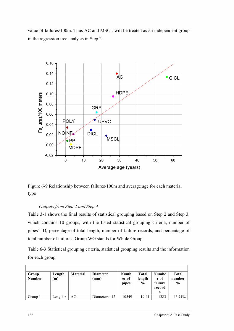
132 Chapter 6: A Case Study
value of failures/100m. Thus AC and MSCL will be treated as an independent group
in the regression tree analysis in Step 2.
Figure 6-9 Relationship between failures/100m and average age for each material type
Outputs from Step 2 and Step 4 Table 3-1 shows the final results of statistical grouping based on Step 2 and Step 3,
which contains 10 groups, with the listed statistical grouping criteria, number of
pipes’ ID, percentage of total length, number of failure records, and percentage of
total number of failures. Group WG stands for Whole Group.
Table 6-3 Statistical grouping criteria, statistical grouping results and the information
for each group
Group Number
Length (m)
Material Diameter (mm)
Number of pipes
Total length
%
Number of
failure record
s
Total number
%
Group 1 Length> AC Diameter<=12 10549 19.41 1383 46.71%
0 10 20 30 40 50 60-0.02
0.00
0.02
0.04
0.06
0.08
0.10
0.12
0.14
0.16
Fajlu
res/
100
met
ers
Average age (years)
CICLAC
HDPE
GRP
MSCLDICL
UPVC
MDPE
POLY
PPNOINF

Chapter 6: A Case Study 133
1 5 Group 2 Length>
1 AC Diameter>125 8106 18.38 532 17.97%
Group 3 Length>1
MSCL All range 1216 3.96 27 0.91%
Group 4 Length>1
CICL, DICL, GRP
Diameter <=105
4838 2.60 84 2.84%
Group 5 Length>1
CICL, DICL, GRP
Diameter >105
9199 12.33 152 5.13%
Group 6 Length>1
UPVC, NOINF
Diameter <=212.5
23516 34.19 613 20.70%
Group 7 Length>1
UPVC, NOINF
Diameter>212.5
3413 6.66 124 4.19%
All pipes All range
All materials
All range 71282 100.00 2960 100.00%
6.3.2 Empirical hazards for each group
Table 6-4 showed the parameters of the fitted hazard curve for each group. The
selected wear-out point, and the estimated parameters for each group, are also shown
on each line. The wear-out point is the point from which the subgroup pipes are
assumed to start aging. For the estimated parameters, ‘lamda’ gives the estimated
exponential rate; ‘Scale’ and ‘shape’ indicate the scale parameter and shape
parameter for the piecewise hazard, respectively.
Note that the determination of the wear-out point and the curve fitting results should
only be considered as one of the many possible reasonable solutions to the grouping
issue because of the complexity of real life data and the limitation of the optimisation
procedure. Therefore, cautions are needed in interpretation and application wherever
these results do not match engineering experience.
Table 6-4 Hazard model parameters for each group Group Number Wear-out point lamda (*10^-5) Scale Shape Group 1 19 9.30 266.93 2.6601 Group 2 35 5.80 1011.45 1.7456 Group 3 25 4.45 5901.17 1.1946 Group 4 25 7.81 6263.19 1.0529 Group 5 52 3.91 208.79 2.2912 Group 6 13 2.90 1514.10 1.4769 Group 7 13 2.30 1806.59 1.2715
Figure 6-10 to Figure 6-16 shows the calculated hazard for each group, the empirical
hazard (blue bar) with fitted piecewise hazard model curve (red line) for each group.

134 Chapter 6: A Case Study
Figure 6-10 Hazard curve for group 1
Figure 6-11Hazard curve for group 2
Figure 6-12 Hazard curve for group 3
0 0.0005 0.001 0.0015 0.002 0.0025 0.003
1 6 11 16 21 26 31 36 41 46 51 56 61 66 71
Hazard
Age (year)
0 5E-‐05 0.0001 0.00015 0.0002 0.00025 0.0003 0.00035 0.0004 0.00045
1 6 11 16 21 26 31 36 41 46 51 56 61 66 71
Hazard
Age (year)
0
5E-‐05
0.0001
0.00015
1 6 11 16 21 26 31 36 41 46 51 56 61 66 71
Hazard
Age (year)

Chapter 6: A Case Study 135
Figure 6-13 Hazard curve for group 4
Figure 6-14 Hazard curve for group 5
Figure 6-15 Hazard curve for group 6
0
0.0002
0.0004
0.0006
0.0008
0.001
0.0012
1 6 11 16 21 26 31 36 41 46 51 56 61 66 71
Hazard
Age (year)
0.00E+00 5.00E-‐05 1.00E-‐04 1.50E-‐04 2.00E-‐04 2.50E-‐04 3.00E-‐04 3.50E-‐04 4.00E-‐04 4.50E-‐04 5.00E-‐04
1 6 11 16 21 26 31 36 41 46 51 56 61 66 71
Hazard
Age (year)
0.00E+00
2.00E-‐04
4.00E-‐04
6.00E-‐04
8.00E-‐04
1.00E-‐03
1.20E-‐03
1 6 11 16 21 26 31 36 41 46 51 56 61 66 71
Hazard
Age (year)
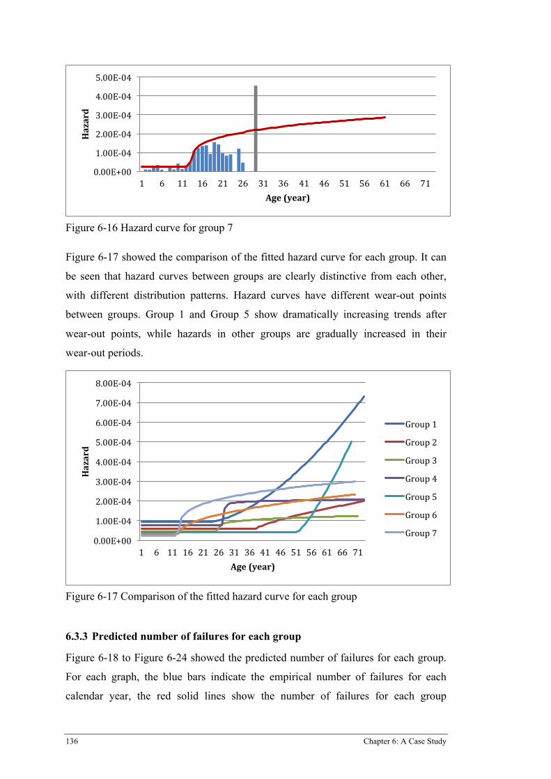
136 Chapter 6: A Case Study
Figure 6-16 Hazard curve for group 7 Figure 6-17 showed the comparison of the fitted hazard curve for each group. It can
be seen that hazard curves between groups are clearly distinctive from each other,
with different distribution patterns. Hazard curves have different wear-out points
between groups. Group 1 and Group 5 show dramatically increasing trends after
wear-out points, while hazards in other groups are gradually increased in their
wear-out periods.
Figure 6-17 Comparison of the fitted hazard curve for each group
6.3.3 Predicted number of failures for each group
Figure 6-18 to Figure 6-24 showed the predicted number of failures for each group.
For each graph, the blue bars indicate the empirical number of failures for each
calendar year, the red solid lines show the number of failures for each group
0.00E+00
1.00E-‐04
2.00E-‐04
3.00E-‐04
4.00E-‐04
5.00E-‐04
1 6 11 16 21 26 31 36 41 46 51 56 61 66 71
Hazard
Age (year)
0.00E+00
1.00E-‐04
2.00E-‐04
3.00E-‐04
4.00E-‐04
5.00E-‐04
6.00E-‐04
7.00E-‐04
8.00E-‐04
1 6 11 16 21 26 31 36 41 46 51 56 61 66 71
Hazard
Age (year)
Group 1
Group 2
Group 3
Group 4
Group 5
Group 6
Group 7

Chapter 6: A Case Study 137
calculated based on the hazard calculated previously and the total pipe length in each
calendar year, and the red dot lines indicates the predicted number of failures for
each group. Since the failure records only have less than ten years failure observation,
which started from 31/06/2002 and ended at 31/06/2012, the number of failures in
2002 and 2012 were only a half year’s observation, therefore, lower values of the
number of failures can be noted at the blue bars at 2002 and 2012.
Figure 6-18 Predicted number of failures for group 1
Figure 6-19 Predicted number of failures for group 2
0
50
100
150
200
2000
2001
2002
2003
2004
2005
2006
2007
2008
2009
2010
2011
2012
2013
2014
2015
2016
2017
2018
2019
2020
Num
ber of failures
Calendar year
0 10 20 30 40 50 60 70
2000
2001
2002
2003
2004
2005
2006
2007
2008
2009
2010
2011
2012
2013
2014
2015
2016
2017
2018
2019
2020
Num
ber of failures
Calendar year

138 Chapter 6: A Case Study
Figure 6-20 Predicted number of failures for group 3
Figure 6-21 Predicted number of failures for group 4
Figure 6-22 Predicted number of failures for group 5
0 1 2 3 4 5 6 7
Num
ber of failures
Calendar year
0 2 4 6 8 10 12 14 16
2000
2001
2002
2003
2004
2005
2006
2007
2008
2009
2010
2011
2012
2013
2014
2015
2016
2017
2018
2019
2020
Num
ber of failures
Calendar year
0 5 10 15 20 25 30 35 40
2000
2001
2002
2003
2004
2005
2006
2007
2008
2009
2010
2011
2012
2013
2014
2015
2016
2017
2018
2019
2020
Num
ber of failures
Calendar year
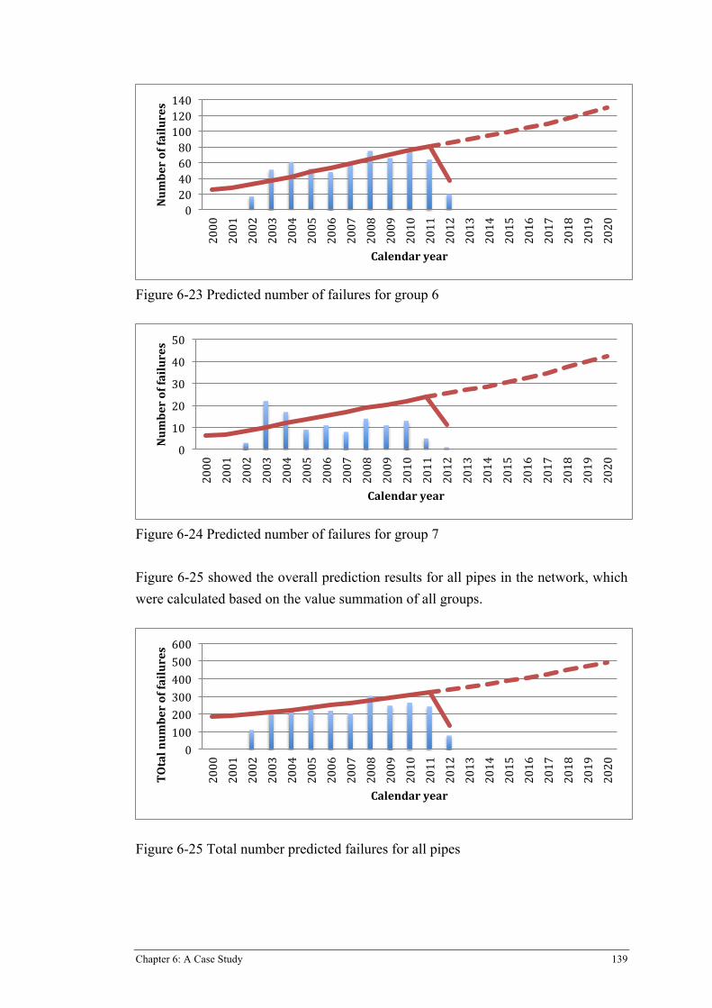
Chapter 6: A Case Study 139
Figure 6-23 Predicted number of failures for group 6
Figure 6-24 Predicted number of failures for group 7 Figure 6-25 showed the overall prediction results for all pipes in the network, which were calculated based on the value summation of all groups.
Figure 6-25 Total number predicted failures for all pipes
0 20 40 60 80 100 120 140
2000
2001
2002
2003
2004
2005
2006
2007
2008
2009
2010
2011
2012
2013
2014
2015
2016
2017
2018
2019
2020
Num
ber of failures
Calendar year
0
10
20
30
40
50
2000
2001
2002
2003
2004
2005
2006
2007
2008
2009
2010
2011
2012
2013
2014
2015
2016
2017
2018
2019
2020
Num
ber of failures
Calendar year
0 100 200 300 400 500 600
2000
2001
2002
2003
2004
2005
2006
2007
2008
2009
2010
2011
2012
2013
2014
2015
2016
2017
2018
2019
2020
TOtal num
ber of failures
Calendar year

140 Chapter 6: A Case Study
Based on the fitted hazard curves for each group, the probability of failures for each
individual pipe at each age can be calculated.
Due to the computational capacity issue, this case study made a reasonable
simplification. Only the pipes, whose probability of failures are higher than 0.01
during next 20 years, are considered in this case study. Therefore, only 2,344 pipes
are left, and those pipes are used for the replacement decision optimisation analysis
in the next section.
6.4 REPLACEMENT DECISION OPTIMISATION FOR GROUP SCHEDULING
6.4.1 Parameters for cost function and service interruption
Parameters of Repair cost 𝑪𝒇𝒂𝒊𝒍
For some types of failure, costs such as direct damage cost, water loss cost, indirect
damage cost and social cost, were not accessible at this stage; in this case study, it is
assumed that the failure cost is equal to repair cost.
The repair cost calculation relied on the repair history records, which was discussed
in section 6.2.3. The pipe segments repair cost records had ten years of observation,
with five different pipe materials, which were AC, CICL, DICL, MSCL, and UPVC.
A statistical analysis was conducted to analyse the relationships between the repair
cost and materials as well as repair cost and diameter. Two box plots are illustrated
in Figure 6-26 and Figure 6-27 to show different materials and diameters of repair
cost data through the smallest cost, lower quartile, mean value, upper quartile, and
the largest cost observation. Figure 6-26 illustrated that the repair cost shows
dramatic differences between MSCL and the other materials. Three reasons caused
the high repair cost of MSCL pipes: 1) the price of this material on its own was much
higher than the other materials; 2) the repair methods and procedure utilized in
MSCL pipes were more complicated than for the other pipes; 3) Most MSCL pipes
are of larger diameters in the (>300mm), which induce higher cost. Moreover, the
other materials showed a similar repair cost in this case, so that one can treat these
four materials as one group, when the impact of material is taken into account.

Chapter 6: A Case Study 141
Figure 6-26 Repair cost by materials
Figure 6-27 Repair cost by pipe diameter Figure 6-27 showed that the repair cost increased with the increase in diameter, the
similar trend shown in other research[65, 126]. Based on the repair data in this case,
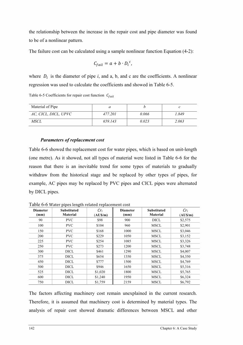
142 Chapter 6: A Case Study
the relationship between the increase in the repair cost and pipe diameter was found
to be of a nonlinear pattern.
The failure cost can be calculated using a sample nonlinear function Equation (4-2):
𝐶!"#$ = 𝑎 + 𝑏 ∙ 𝐷!! ,
where 𝐷! is the diameter of pipe i, and a, b, and c are the coefficients. A nonlinear
regression was used to calculate the coefficients and showed in Table 6-5.
Table 6-5 Coefficients for repair cost function 𝐶!"#$
Material of Pipe a b c
AC, CICL, DICL, UPVC 477.201 0.066 1.849
MSCL 659.143 0.023 2.063
Parameters of replacement cost
Table 6-6 showed the replacement cost for water pipes, which is based on unit-length
(one metre). As it showed, not all types of material were listed in Table 6-6 for the
reason that there is an inevitable trend for some types of materials to gradually
withdraw from the historical stage and be replaced by other types of pipes, for
example, AC pipes may be replaced by PVC pipes and CICL pipes were alternated
by DICL pipes.
Table 6-6 Water pipes length related replacement cost Diameter
(mm) Substituted
Material Cri
(AU$/m) Diameter
(mm) Substituted
Material Cri
(AU$/m) 90 PVC $98 900 DICL $2,575
100 PVC $104 960 MSCL $2,901 150 PVC $168 1000 MSCL $3,046 200 PVC $229 1050 MSCL $3,152 225 PVC $254 1085 MSCL $3,326 250 PVC $273 1200 MSCL $3,748 300 DICL $461 1290 MSCL $4,007 375 DICL $654 1350 MSCL $4,350 450 DICL $777 1500 MSCL $4,769 500 DICL $946 1650 MSCL $5,316 525 DICL $1,020 1800 MSCL $5,765 600 DICL $1,240 1950 MSCL $6,324 750 DICL $1,759 2159 MSCL $6,792
The factors affecting machinery cost remain unexplained in the current research.
Therefore, it is assumed that machinery cost is determined by material types. The
analysis of repair cost showed dramatic differences between MSCL and other

Chapter 6: A Case Study 143
materials. Considering these dramatic differences, the machinery cost was taken as
M=AU$4,000/unit for MSCL and M=AU$2,000/unit for other materials. The
distance-unit cost, Cvi, was set to AU$100/km. The total budget for replacement of
the whole water distribution network was AU$40 million for the next 20 years. Users
based on their circumstances can change all these cost values.
Customer interruption
Customer interruption is a key factor, which is a concern for water utilities for their
repair and replacement activities. In this case study, the water utility provided the
information for customer interruption with Pipe ID, number of customers affected,
NC,i, customer types for each pipe, and the impact factors for customer types.
The classification of customer types was based on the population data from the water
utility, which contained four types, CBD, High Density Urban, Urban and Rural. The
category-specific impact factor fC,i is shown in Table 6-7.
Table 6-7 Category-specific Impact Factor
Category CBD HIGH DENSITY URBAN URBAN RURAL
fiC 4.43 3.43 2.26 1.00
The duration of service interruption of each replacement pipe i, DrC,i, depends on the
workload and work efficiency. In practice, the workload and efficiency is not only
related to the machinery and skilled labour, but also relies on the diameter and length
of pipes. In this case study, the duration per metre replacement DrC is assumed and
listed in Table 6-8.
Table 6-8 Service Interruption Duration
Diameter (mm) <300 300-900 >900 DrC hour/meter 1 2 3
6.4.2 Judgment matrix
In this case, the maximum geographic distance γ* was determined through
calculating the distance between the nine maintenance centres. The minimum
distance among the nine maintenance centres was 8.6km. Replacement of one group
of pipes is assumed be accomplished by only one maintenance team from only one

144 Chapter 6: A Case Study
maintenance centre. Therefore, the maximum geographic distance γ* was assumed to
be 4.3km.
The answers to the question, “which types of machinery are suitable for particular
pipes?” rely on the expert knowledge of the engineers from water utilities and
replacement contractors. All replacement activities, in this case study, are assumed
be open trench replacement, so that the machinery utilised for each pipe relies on the
pipe’s diameter and material. To simplify this relationship, the machinery utilisation
is treated following the hazard statistical grouping results calculated in section 6.3,
which means that replacement pipes in the same hazard group can use the same
machinery. Therefore, if pipe i and pipe j in the same hazard group, 𝜀!"!" = 0,
otherwise, 𝜀!"!" = 1.
Since the water utility in this case study cannot provide any hydraulic information,
therefore, if pipe i and pipe j share the same node (for example, valves), 𝑁!,!,! =
max (𝑁!,! ,𝑁!,!), otherwise 𝑁!,!,! = 0.
Based on the group scheduling analysis, the judgment matrix for the 2,344 pipes,
which is a “2344 by 2344” matrix with square matrix with values between 0 and 1,
which showed in Figure 6-28 with colours, black indicated “0” and red indicated “1”.
Figure 6-28 Judgment matrix
0
0.1
0.2
0.3
0.4
0.5
0.6
0.7
0.8
0.9
1

Chapter 6: A Case Study 145
6.4.3 Parameters for the modified NSGA-II
The modified NSGA-II was given integer-valued decision variables. The population
size, pop, is set as 100, the maximum generation is set as 500. 2,344 pipes are
considered (𝑛 = 2,344), therefore, there are 2,344 design variables. Maximum
number of pipes in each group, 𝑔𝑚𝑎𝑥 = 5. Therefore the lower and upper bounds
are 𝐱(!) = 1,… ,1 , and 𝐱(!) = 2,344,… ,2,344 . The number of objective
function is 2.
A crossover probability of pc = 0.8 and in the mutation operator, the standard
deviation 𝜎! = 2, 𝜌 = 0.3 . In the selection operator, the selective pressure,
𝑆𝑃 = 1.1.
6.4.4 Results and discussions
Figure 6-29 provided the Pareto-front of the optimized solution for group scheduling
replacement. Vertical and horizontal axes indicate the values of the two objectives,
minimizing total life-cycle cost and minimizing service interruption impact,
respectively. The AU$40 million budget is marked with red solid line. The area
inside the Pareto-front and the total budget line is the feasible solution area, which
means that all solutions located outside of this area are impossible or unacceptable.
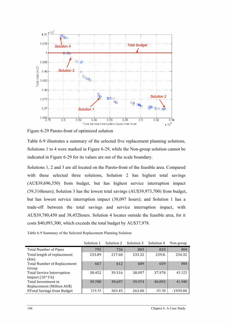
146 Chapter 6: A Case Study
Figure 6-29 Pareto-front of optimized solution
Table 6-9 illustrates a summary of the selected five replacement planning solutions,
Solutions 1 to 4 were marked in Figure 6-29, while the Non-group solution cannot be
indicated in Figure 6-29 for its values are out of the scale boundary.
Solutions 1, 2 and 3 are all located on the Pareto-front of the feasible area. Compared
with these selected three solutions, Solution 2 has highest total savings
(AU$39,696,550) from budget, but has highest service interruption impact
(39,316hours); Solution 3 has the lowest total savings (AU$39,973,700) from budget,
but has lowest service interruption impact (38,097 hours); and Solution 1 has a
trade-off between the total savings and service interruption impact, with
AU$39,780,450 and 38,452hours. Solution 4 locates outside the feasible area, for it
costs $40,093,300, which exceeds the total budget by AU$37,978.
Table 6-9 Summary of the Selected Replacement Planning Solution
Solution 1 Solution 2 Solution 3 Solution 4 Non-group
Total Number of Pipes 795 736 803 810 804 Total length of replacement (km)
233.89 217.60 233.32 239.8. 234.32
Total Number of Replacement Group
667 612 689 659 804
Total Service Interruption Impact (10^3 h)
38.452 39.316 38.097 37.978 43.325
Total Investment in Replacement (Million AU$)
39.780 39.697 39.974 40.093 41.940
0Total Savings from Budget 219.55 303.45 263.00 -93.30 -‐1939.00

Chapter 6: A Case Study 147
(10^3 AU$) An optimization of replacement planning without considering grouping schedule
(non-group schedule) was also conducted for comparing the results of the group
scheduling replacement planning. The lowest expected total investment of non-group
schedule was AU$41,939,000, which is AU$1,939,909 greater than the total budget
(AU$40 million). Moreover, for non-group schedules, the total service interruption
impact can be as high as 43325hours.
Table 6-10 provides the details of the replacement planning of Solution 1 from 1st to 20th year.
Table 6-10 Summary of the replacement planning of Solution 1
Y
Total Number of Pipe
Total length of
replacement (m)
Total length of
replacement
Total Number of
Replacement Groups
Total Service Interruption Impact (h)
Total Investment in Replacement
(AU$)
1 7 2614 1.12% 7 338.6 444,593 2 12 3526 1.51% 12 580.4 599,707 3 11 2875 1.23% 11 532.0 488,984 4 26 8307 3.55% 25 1,257.5 1,412,866 5 25 7224 3.09% 21 1,209.2 1,228,668 6 30 8627 3.69% 30 1,451.0 1,467,292 7 39 12278 5.25% 31 1,886.3 2,088,260 8 65 18649 7.97% 52 3,143.9 3,171,848 9 63 19987 8.55% 55 3,047.1 3,399,417
10 67 17031 7.28% 55 3,240.6 2,896,656 11 90 26809 11.46% 67 4,353.1 4,559,712 12 70 19697 8.42% 48 3,385.7 3,350,093 13 67 19212 8.21% 57 3,240.6 3,267,604 14 64 17764 7.60% 51 3,095.5 3,021,326 15 52 17041 7.29% 46 2,515.1 2,898,357 16 41 11317 4.84% 36 1,983.1 1,924,811 17 32 11247 4.81% 30 1,547.8 1,912,906 18 17 5260 2.25% 17 822.2 894,628 19 17 4423 1.89% 16 822.2 752,270
Total 795 233888 100% 667 38,452 39,780,450
Table 6-11 shows the details of the first year replacement planning of Solution 1. 7
pipes should be replaced in seven grouped replacement activities, which means that
the seven pipes should be replaced individually.
Table 6-11 Details of the first year replacement planning of Solution 1 Group No. Asset key (Pipe ID) Length of pipe 1 530589 325.44 2 519636 238.99 3 525748 732.63

148 Chapter 6: A Case Study
4 1091733 239.58 5 500010 278.16 6 533172 172.63 7 500237 626.52
For the seventh year replacement planning, a greater value of pipe numbers
compared with group number can be noticed, which means some pipes should be
grouped together as one replacement activity. Table 6-12 listed 11 pipes at the
seventh year of Solution 1. For example, pipes with asset keys “507185” and
“512619” should be treated in one group, and pipes with asset keys “512183” and
“513351” and “529450” should be grouped as well.
Table 6-12 Examples of the seventh year replacement planning of Solution 1 Group No. Construction Date Material Diameter Pipe Length 1 01/07/1997 UPVC 100 172.1153 1 01/07/1979 AC 100 144.9601 2 01/07/1980 AC 100 469.2863 3 01/07/1974 AC 100 193.6723 3 01/07/1984 AC 100 96.2167 3 01/07/1968 AC 225 92.8967 4 01/07/1995 UPVC 150 208.6306 4 01/07/1987 AC 100 381.8578 5 01/07/1988 AC 225 1094.0596 6 01/07/1992 UPVC 100 300.8922 7 01/07/1957 AC 100 416.1085 … … … … …
6.5 DISCUSSIONS
This case study followed the three-step process: (1) a data pre-analysis to investigate
the provided data, to exclude invalid data, and to analyse the general characteristics;
(2) a statistical grouping-based hazard prediction analysis to partition data into
different subgroup based on their homogeneity, to calculate empirical hazard for
each subgroup, and to fit hazard curve for failure prediction; (3) a replacement
decision optimisation for group scheduling that gives an optimised replacement
planning, taking total cost and customer interruption into consideration.
The first part, data pre-analysis, filtered the real data from the water utility and
discarded the invalid data. A summary of the water pipe network was delivered. In
the second part, seven pipe groups for hazard calculation were developed based on
the statistical grouping analysis, followed by the hazard prediction for the seven

Chapter 6: A Case Study 149
groups. The probability of failure for each individual pipe was predicted. Then to
simplify the computation, pipes with high probability of failures were retained for the
replacement optimisation analysis.
The third part, replacement optimisation analysis, provided a graph (Figure 6-29) of
Pareto-front of the optimized solution for replacement planning of group scheduling.
Figure 6-29 showed a feasible solution area, which considered the trade-offs between
the two objectives. Replacement operators can make decisions based on their own
requirements by selecting one solution located in the Pareto-front, from which the
five representative solutions were listed in Table 6-9 for comparison. The results
illustrated that the group scheduling solutions (Solution 1, 2 and 3) can reduce the
total life-cycle cost for approximately 5% compared with the non-group scheduling
solution. Moreover, replacement group scheduling also contributes to dealing with
overlapping water discontinuity areas. As a result, the total service interruption
impact can dramatically shrink approximately 11.25%.

Chapter 6: A Case Study 150
Chapter 7: Conclusions and Future Work 151
Chapter 7: Conclusions and Future Work
Water pipeline replacement plays a vital role in controlling water pipe failures,
infrastructure budgeting, and the level of services to the community. Reliability
analysis and replacement optimisation lead to better replacement scheduling of water
pipelines. This candidature has developed practical models and methodologies for
water pipelines to provide advanced economic replacement schedules to meet the
requirements of reduced costs and service interruptions.
After an extensive literature review, the candidate identified the following limitations
in the work conducted to date:
(1) From a thorough literature review, it appears that the optimisation of group
replacement scheduling of water pipelines has not been modelled previously.
Existing models and methodologies have primarily focused on individual/single
pipes to provide replacement schedules, which deliver an optimal replacement
time. These methodologies do not satisfy the requirements of group replacement
schedules of pipelines that would improve replacement efficiency and reduce
replacement costs.
(2) Sometimes, evolutionary algorithms are applied to optimise replacement
scheduling. However, these algorithms do not cater for group scheduling of pipes.
They are only valid for individual/single pipes. The optimisation of scheduling
groups of pipes needs to consider both time and space domains, while the work
involving evolutionary algorithms have only focused on the time domain.
(3) In reliability prediction, existing hazard-based modelling methods have
limitations when applied to real-world water pipes. They are limited when it
comes to handling multiple failure characteristics, mixed failure distributions as
well as lifetime data that would be truncated.
In this thesis, the candidate endeavoured to overcome these limitations and
developed the following new methodologies/models:
(1) An optimization model for group replacement schedules of water pipelines -
referred to as RDOM-GS. RDOM-GS integrates reliability analysis, cost
152 Chapter 7: Conclusions and Future Work
analysis, service interruption analysis, and optimization analysis to deliver
optimal water pipes group replacement schedules, in terms of reduced service
interruptions and total life-cycle costs.
(2) A modified NSGA-II to deal with the challenges of the allocations of pipelines
for group replacement scheduling.
(3) An improved hazard-based modelling method for predicting the reliability of
water pipelines taking into account multiple failure characteristics, mixture of
failure distributions, and truncated lifetime data.
This chapter summarises the candidate’s work and highlights its contributions to the
knowledge in reliability analysis and replacement decision optimisation of water
pipelines. Future research directions are also discussed.
7.1 SUMMARY OF RESEARCH
This candidature developed an optimization model for group replacement schedules
of water pipelines, known as RDOM-GS with the following components:
• Three criteria of group scheduling which considers geographic distance,
machinery utilisation and service interruptions a judgment matrix is used to
quantify these three criteria.
• A cost model including repair cost, replacement cost and the net present value
of total cost that considers the effects of group scheduling.
• A model of service interruption, which calculates customer impact due to
each replacement activity. The impact is derived using the number of
customers, the type of customers and the duration of the interruption.
• A modified NSGA-II, which deals with multi-objective replacement
optimisation considering group scheduling. The modification contains a new
designed encoding method to present the group number and replacement year
of each pipe, a crowding distance operator to enhance the diversity in the
solutions of the Pareto-optimal set, a mutation operator to keep pipes
scheduled in one group that can be replaced in the same year.
This candidature also developed an improved hazard-based modelling method for
water pipe reliability analysis, which comprises three components.

Chapter 7: Conclusions and Future Work 153
• The first component is a grouping algorithm using regression trees and expert
rules, which partitioned the total number of water pipes into relatively
homogeneous groups. This algorithm was validated using a case study based
on selected water pipes data sets from a water utility.
• The second component is a suitable empirical hazard formula for water pipes
derived from one of two different hazard formulas. The appropriate function
was selected by the investigation of their different application impacts based
on theoretical analysis and simulation experiments.
• The third component is a modified empirical hazard function to deal with the
underestimation effects due to truncated lifetime data, which was validated
using a Monte Carlo simulation framework developed in the candidature and
which was based on a real water utility. Test-bed sample data sets were
generated based on the main features of the real data of a water utility to test
and validate the proposed improved empirical hazard function.
Both RDOM-GS and the improved hazard-based model was evaluated using a
case study based on the maintenance of a local water utility responsible for almost
3,000 km of underground water pipes to test and apply the two models. The case
study started with a data pre-analysis to ensure the quality of data, and analysed the
age profile as well as repair history of the water pipes. A grouping analysis was
presented using the grouping algorithm to partition pipes into seven groups. The
empirical hazards were calculated followed by the parameters estimation for each
partitioned group. RDOM-GS was utilised to optimise the replacement decision
based on group scheduling.
7.2 RESEARCH CONTRIBUTIONS
This thesis presents several contributions in the field of optimisation for replacement
scheduling of water pipelines and hazard modelling for reliability prediction. Three
of these major contributions are summarised in the following subsections.
7.2.1 Multi-objective multi-criteria optimisation for group replacement schedules
This candidature developed RDOM-GS, which considered multiple optimisation
objectives and multiple scheduling criteria. RDOM-GS has the following four
characteristics:

154 Chapter 7: Conclusions and Future Work
Multi-criteria group scheduling for water pipeline replacement
Water pipeline replacement is usually scheduled in groups manually in order to
reduce cost. However, research into group scheduling for water pipeline replacement
considering multiple criteria for optimisation appears to be absent in the literature.
The proposed RDOM-GS fills this gap by considering three criteria: geographic
distance, machinery utilisation and service interruption, which are quantified by the
judgment matrix.
Cost model for groups of pipelines
The new cost model considers the trade-off between repair costs and replacement
costs. The Repair cost function was developed through the analysis of real repair cost
data using nonlinear regression, while the Replacement cost function was developed
considering length related cost, machinery cost and transportation cost. Each
component can be altered with different group scheduling solutions. The total cost is
the sum of repair costs and replacement costs considering failure probability and Net
Present Value (NPV) – the latter, which is applied as one of the objectives of the
replacement optimisation.
Customer interruption model for groups of pipelines
Similar to the cost model, despite a thorough literature search that evidence of
research work on customer interruption factors for group scheduling is missing. In
this candidature, a new customer interruption model, which considered the number of
customers interrupted, the type of customers and the duration of interruption was
developed as part of RDOM-GS. This service interruption model integrates failure
probability and the customer impact caused by groups of pipes.
Optimisation algorithm for scheduling groups of pipelines
Group scheduling for water pipeline replacement optimisation is complex, as it needs
to consider a large number of decision variables, which are in both time and space
domains. Existing optimisation methods cannot be applied directly to deliver optimal
solutions. RDOM-GS integrates a modified NSGA-II to deal with this multiple
criteria and multiple objective optimisation problems. The modified NSGA-II
enables RDOM-GS to deliver schedules in order to limit service interruptions and to
minimize total life-cycle cost. Results from a comparison study showed that the
modified NSGA-II produced better optimised replacement schedules, with lower
Chapter 7: Conclusions and Future Work 155
total cost, lower service interruption and greater diversity in the solutions of the
Pareto-optimal set.
7.2.2 Improved Hazard modelling methods for water pipelines
The improved hazard modelling method, developed in this candidature, contributes
to the knowledge of reliability prediction for water pipelines in three aspects:
A systematic grouping algorithm for water pipes
The grouping algorithm developed in this candidature can effectively analyse water
pipe data with multiple failure distributions. The four-step procedure of the statistical
grouping algorithm consists of (1) an age-specific material analysis to calculate the
number of failures per unit-length over average age for each material type; (2) length
related pre-grouping; (3) regression tree analysis to partition pipe data considering
material type, diameter and length; and (4) grouping criteria adjustment based on
knowledge rules.
Using this procedure, pipe data can be partitioned into relatively homogeneous
groups, and sufficient sample size of failure data for each group can be guaranteed.
Based on the grouping algorithm, the hazard curves between groups can be clearly
distinctive from each other; hence, more accurate hazard prediction results for each
group of pipes can be derived.
Critical evaluation of two frequently used empirical hazard formulas
The differences of application impacts between two commonly used empirical
hazard formulas ℎ1! and ℎ2! (Equations (3-9) and (3-10)) have not been clearly
reported in the literature. Overlooking this difference may result in inaccuracies in
the calculations. This candidature conducted a comprehensive evaluation on
estimated performance of the two formulas against true hazard function values
through theoretical analysis and simulations, with the following conclusions:
1) ℎ2! is a finite approximation of average failure rate (AFR), whereas ℎ1! is
a finite approximation of the instantaneous failure rate. However, when time
interval ∆𝑡 approaches zero, both ℎ1! and ℎ2! converge to the true
hazard function;
2) Theoretically, the difference between formulas ℎ1! and ℎ2! is significant.
ℎ1! underestimates the true hazard function values in most cases and the

156 Chapter 7: Conclusions and Future Work
underestimation is substantial, while ℎ2! gives much less biased estimation
of the true hazard function than ℎ1!;
3) For data analysis purposes, the underestimation of ℎ1! is much more
sensitive to the change of time interval ∆𝑡, while ℎ2! is almost not affected.
Therefore, for calculating empirical hazard function of continuous-time
failure data, if the maximum failure rate over the time interval periods is less
than 0.1, both formulas are good estimators of the true hazard function
values. Otherwise, ℎ2! has a higher accuracy result than ℎ1! for
calculating the empirical hazard function.
Modified empirical hazard model considering truncated lifetime data
The field lifetime data for water pipes is often truncated. This truncation results in
the underestimation of the true hazard when calculating the empirical hazard. The
modified empirical hazard function based on pipe segmentation considers three types
of pipe segments: survived pipe segments, repaired pipe segments and new pipe
segments. The Monte Carlo simulation framework developed in this candidature
enables to generate test-bed sample data sets in terms of the main features of the real
data of a water utility. By applying this simulation framework to generate test-bed
sample data, the modified empirical hazard function has been verified that it can
effectively reduce the underestimation effects caused by truncated lifetime data, by
can effectively reduce the underestimation effects caused by the interval truncation
of lifetime data.
7.2.3 Application of the proposed models in a real case study
The real case study involved the application of the proposed improved hazard model
and RDOM-GS to a water utility responsible for almost 3,000 km of water pipelines.
All pipelines were partitioned into seven groups using the grouping algorithm. For
each group, the calculated empirical hazards were calculated in specific patterns. The
real values of the number of failure in each calendar year showed that the proposed
improved hazard-based modelling method provided good estimation results for water
pipe failure prediction.
Application of the RDOM-GS resulted in a Pareto-optimal set and a set of scheduled
replacement activities, which included the information of the water pipe’s unique ID,
group number, replacement year, total cost and total service interruption.

Chapter 7: Conclusions and Future Work 157
Additionally, total life-cycle costs reduced by AU$ 2.16 million (approximately 5%)
compared with the non-group scheduling solution, and total service interruptions
shrunk by11.25%.
7.3 FUTURE RESEARCH DIRECTIONS
The RDOM-GS and the improved hazard modelling method can be further improved
or extended as follows:
7.3.1 Extension of multi-objective RDOM-GS
This candidature provides a model of optimisation for group replacement schedules
of water pipelines. Two objectives were considered as minimum the total life cycle
costs and service interruption impacts. However, there are some other important
issues for water utilities that need to be considered for replacement scheduling, for
example, the leakage of water pipeline caused high levels of non-revenue water
(NRW). High levels of NRW are detrimental to the financial viability of water
utilities, as well to the quality of water itself. Therefore, the RDOM-GS can be
further extended considering improvement of water quality or hydraulic
performance.
Moreover, current RDOM-GS considered pipeline replacement as replacing the
whole length of pipeline. However, for some pipelines, especially those of long
length, replacement of one part of the pipe rather than the whole length seems more
reasonable, because failures may only happen in a small area rather than being
distributed over the whole length. This improvement requires the failure records to
be more precise in positions and locations.
7.3.2 Extension of hazard modelling method for water pipes
The candidate developed an improved hazard modelling method to improve the
existing hazard model [13] in satisfying three aspects: the requirement for
partitioning pipe into relatively homogeneous groups based on specific features of
water pipes, the requirement for dealing with underestimation effects caused by
truncated lifetime data, and the requirement for differentiating two commonly used
empirical hazard formulas. However, failure, in this candidature, is only considered
as general failure, which is not categorised based on different specific failure modes.
Different failure modes might be caused by different reasons, that may lead to

158 Chapter 7: Conclusions and Future Work
different types of works, e.g. repair, inspection, condition monitoring. Therefore,
hazard-modelling methods can be further extended to predict the reliability of a
water pipe system in the following scenarios:
• Hazard modelling method considering multiple failure modes (e.g. break,
rupture, leakage, corrosion)
• Hazard modelling method with multiple types of works (e.g. repair, inspection)
Moreover, the generation of the simulation samples based on the proposed Monte
Carlo simulation framework is efficient for practical data analysis purpose. However,
this simulation has only considered pipe length as pipe’s feature. This simulation
sample generation algorithm may be further developed for testing the impact of
possible covariates e.g. material types, diameter and soil types on the asset failure
patterns in the future.
7.3.3 Application to other linear assets
Water pipelines are linear infrastructure assets. All linear infrastructure assets have
similar features, such as being spanned in long distances, various working
environments, having different failure rates, and replacement considering group
scheduling. These features lead to similar methods for all linear assets to deal with
hazard calculation and replacement optimization, compared with the methods for
water pipelines. Therefore, the proposed improved hazard model and the RDOM-GS
have the potential to optimize maintenance planning in other linear asset networks
such as electricity distribution, railway networks and road networks.
7.4 FINAL REMARKS
In today’s market, water utilities strive to operate under ever-increasing cost
pressures. Water pipelines are the largest investment for water utilities. The majority
of water utilities today focus their operations on optimizing water pipeline
maintenance to reduce costs. As mentioned in the introductory chapter of this thesis,
maintenance costs have increased dramatically to a level that utilities can no longer
absorb.
Optimisation for group replacement schedules of water pipelines should consider a
multitude of criteria and factors including risk, service interruption, network

Chapter 7: Conclusions and Future Work 159
reliability, resource availability and costs, pipe specifications, and technology to be
employed.
The methodologies and models reported in this thesis would enable maintenance
planners to develop group replacement schedules of groups of pipelines based on
multiple group scheduling criteria considering multiple objectives.
The outputs of this candidature have the potential to optimise replacement planning
in other linear asset networks such as electricity distribution, railway networks and
road networks, resulting in bottom-line benefits for end users and communities.


Bibliography 161
Bibliography
1. Uni-Bell PVC Pipe Association. watermainbreakclock. 2012. 2. AWWA, Dawn of the Replacement Era: Reinvesting in Drinking Water
Infrastructure, 2001, American Water Works Association: Denver, CO. 3. AWWA, Buried No Longer: Confronting America’s Water Infrastructure
Challenge, 2012, American Water Works Association: Denver, CO. 4. Jowitt, P.W. and C. Xu, Predicting pipe failure effects in water distribution
networks. Journal of Water Resources Planning and Management Division, 1993. 119(1): p. 18-31.
5. Li, D. and Y.Y. Haimes, Optimal maintenance related decision making for deteriorating water distribution systems - 2 Multilevel decomposition approach. Water Resources Research, 1992b. 28(4): p. 1053-1061.
6. Dandy, G.C. and M.O. Engelhardt, Multi-Objective Trade-Offs between Cost and Reliability in the Replacement of Water Mains. Journal of Water Resources Planning and Management, 2006. 132(2): p. 79-88.
7. Lansey, K.E., et al., Optimal maintenance scheduling for water distribution systems. Civil Engineering Systems, 1992. 9(211-226).
8. Kleiner, Y. and B.J. Adams, WATER DISTRIBUTION NETWORK RENEWAL PLANNING. Journal of Computing in Civil Engineering, 2001. 15(1): p. 15.
9. Zhang, D. Risk Based Replacement Model of Critical Water Mains. in ICOMS Asset Management Conference. 2010. Adelaide, Australia.
10. Halhal, D., et al., Water network rehabilitation with a structured messy genetic algorithm. Journal of Water Resources Planning and Management Division, 1997. 123(3): p. 137-146.
11. Moglia, M., S. Burn, and S. Meddings, Decision Support System for Water Pipeline Renewal Prioritisation. ITcon Special Issue Decision Support Systems for Infrastructure Management 2006. 11: p. 237-256.
12. Elsinore, M. and F. Jeffery. Optimized Pipe Renewal Programs Ensure Cost-Effective Asset Management. 2011. ASCE.
13. Sun, Y., F. Colin, and L. Ma. Reliability Prediction of Long-lived Linear Assets with Incomplete Failure Data. in ICQRMS2011. 2011. Xian China.
14. Davison, A.C., Statistical Models. 2003: Cambridge University Press. 15. Elsayed, E.A., Reliability Engineering. 1996: Reading, Massachusetts:
Addison Wesley Longman, Inc. 16. Rai, B. and N. Singh, Hazard rate estimation from incomplete and unclean
warranty data. Reliability Engineering & System Safety, 2003. 81: p. 79-92. 17. Conlin, T. Three burst water mains in less than 24 hours has sparked fresh
calls for better maintenance of Adelaide's ageing infrastructure. 2012. 18. Calligeros, M. Water pipe ruptures, splitting city street. 2010. 19. Chisholm, A. Two burst water mains create a water shortage in Brisbane's
north eastern suburbs 2011. 20. ABC news. Burst water main floods Adelaide main road. 2012. 21. ABC news. Burst main in King William Street. 2012.

162 Bibliography
22. Yamine, E. Sydney street turned into river. 2012. 23. ABC news. Burst main shoots water 50 metres high. 2012. 24. WSAA, Common Failure Modes in Pressurised Pipeline Systems, 2003,
Water Services Association of Australia: Melbourne. 25. Røstum, J., STATISTICAL MODELLING OF PIPE FAILURES IN WATER
NETWORKS, in Department of Hydraulic and Environmental Engineering2000, Norwegian University of Science and Technology NTNU: Trondheim, Norway.
26. Hu, Y. and D.W. Hubble, Factors contributing to the failure of asbestos cement water mains. Canadian Journal of Civil Engineering, 2007. 34(5): p. 608-621.
27. Davis, P., et al., A physical probabilistic model to predict failure rates in buried PVC pipelines. Reliability Engineering & System Safety, 2007. 92(9): p. 1258-1266.
28. Millette, L. and D.S. Mavinic, The Effect of pH on the Internal Corrosion Rate of Residential Cast-Iron and Copper Water Distribution Pipes. Canadian Journal of Civil Engineering, 1988. 15: p. 79-90.
29. Stewart, L., Alaskan Pipeline Embraces Prevention. Construction Equipment, 2005. 108(6): p. 58-59.
30. Insituform awarded contracts for pipeline projects. Underground Construction, 2009. 64(9): p. 66-66.
31. Durban water pipe replacement project nears completion, in Trenchless International2010.
32. WaterWorld. Pipe replacement project in Russell, KS, gets EPA funding. 2011.
33. Ramakumar, R., Engineering reliability: fundamentals and applications. 1993: Prentice Hall.
34. Kleiner, Y. and B. Rajani, Comprehensive review of structural deterioration of water mains: statistical models. Urban Water, 2001. 3(3): p. 131-150.
35. Park, S., et al., Modeling of Water Main Failure Rates Using the Log-linear ROCOF and the Power Law Process. Water Resources Management, 2008. 22(9): p. 1311-1324.
36. Wang, Y., T. Zayed, and O. Moselhi, Prediction Models for Annual Break Rates of Water Mains. Journal of Performance of Constructed Facilities, 2009. 23(1): p. 47-54.
37. Fahmy, M. and O. Moselhi, Forecasting the Remaining Useful Life of Cast Iron Water Mains. Journal of Performance of Constructed Facilities, 2009. 23(4): p. 269-275.
38. Jafar, R., I. Shahrour, and I. Juran, Application of Artificial Neural Networks (ANN) to model the failure of urban water mains. Mathematical and Computer Modelling, 2010. 51(9–10): p. 1170-1180.
39. Syachrani, S., H. Jeong, and C. Chung, Dynamic Deterioration Models for Sewer Pipe Network. Journal of Pipeline Systems Engineering and Practice, 2011. 2(4): p. 123-131.
40. Kleiner, Y. and B.B. Rajani, I-WARP: Individual Water Main Renewal Planner. Drinking Water Engineering, 2010. 3: p. 71-77.
41. Sun, Y., et al. Renewal Decision Support for Linear Assets. in Proceedings of the 5th World Congress on Engineering Asset Management (WCEAM2010). 2010. Brisbane, Australia: Springer.

Bibliography 163
42. Jonkergouw, P.M.R., et al., Infrastructure Risk Management: A Probabilistic Approach to Asset Management. 2012.
43. Kleiner, Y. and B.B. Rajani, Using limited data to assess future needs. Journal (American Water Works Association), 1999. 91(7): p. 47-61.
44. Alfelor, R., W. Hyman, and G. Niemi, Customer-Oriented Maintenance Decision Support System: Developing a Prototype. Transportation Research Record, 1999. 1672(1): p. 1-10.
45. Sun, Y., L. Ma, and J. Morris, A practical approach for reliability prediction of pipeline systems. European Journal of Operational Research, 2009. 198(1): p. 210-214.
46. Tan, C.M. and N. Raghavan, A framework to practical predictive maintenance modeling for multi-state systems. Reliability Engineering & System Safety, 2008. 93(8): p. 1138-1150.
47. Bishop, T.N., FRP-LOSS-PREVENTION THROUGH PREDICTIVE MAINTENANCE ENGINEERING. Pulp & Paper-Canada, 1992. 93(6): p. 62-65.
48. Liu, Z. and Y. Kleiner, State of the art review of inspection technologies for condition assessment of water pipes. Measurement, 2013. 46(1): p. 1-15.
49. Shamir, U. and C.D.D. Howard, An Analytical Approach to Scheduling Pipe Replacement. Journal of American Water Works Association, 1979. 71(5): p. 248-258.
50. Li, D. and Y.Y. Haimes, Optimal maintenance related decision making for deteriorating water distribution systems 2 Multilevel decomposition approach. Water Resources Research, 1992b. 28(1).
51. Kim, J.H. and L.W. Mays, Optimal rehabilitation model for water distribution systems. Journal of Water Resources Planning and Management Division ASCE, 1994. 120(5).
52. Kleiner, Y., B.J. Adams, and J.S. Rogers, Selection and scheduling of rehabilitation alternatives for water distribution systems. Water Resources Research, 1998. 34(8).
53. Engelhardt, M.O., Development of A Strategy for the Optimum Replacement of Water Mains, in Department of Civil and Environmental Engineering1999, University of Adelaide. p. 514.
54. Lansey, K.E., et al., Optimal Maintenance Scheduling For Water Distribution Systems. Civil Engineering Systems, 1992. 9(3): p. 211-226.
55. De Schaetzen, W., et al. A genetic algorithm approach for rehabilitation in water supply systems. in Proceedings of the international conference on rehabilitation technology for the water industry. 1998. Lille, France.
56. Deb, A.K., et al., Quantifying Future Rehabilitation and Replacement Needs of Water Mains. AWWA Research Foundation, 1998: p. 156.
57. Ramirez-Rosado, I.J. and J.L. Bernal-Agustin, Reliability and costs optimization for distribution networks expansion using an evolutionary algorithm. IEEE Transactions on Power Systems, 2001. 16(1): p. 111-118.
58. Hastak, M., S. Gokhale, and V. Thakkallapalli, Decision model for assessment of underground pipeline rehabilitation options. Urban Water Journal, 2004. 1(1): p. 27-37.
59. Halhal, D., et al., Water network rehabilitation with a structured messy genetic algorithm. Journal of Water Resources Planning and Management Division ASCE, 1997. 123(137): p. 146.

164 Bibliography
60. Farmani, R., D.A. Savic, and G.A. Walters, Evolutionary multi-objective optimization in water distribution network design. Engineering Optimization, 2005. 37(2): p. 167-183.
61. Raziyeh, F., A.W. Godfrey, and A.S. Dragan, Trade-off between Total Cost and Reliability for Anytown Water Distribution Network. Journal of Water Resources Planning and Management, 2005. 131(3): p. 161-171.
62. Alvisi, S. and M. Franchini, Near-optimal rehabilitation scheduling of water distribution systems based on a multi-objective genetic algorithm. Civil Engineering and Environmental Systems, 2006. 23(3): p. 143 - 160.
63. Atiquzzaman, M., L. Shie-Yui, and Y. Xinying, Alternative Decision Making in Water Distribution Network with NSGA-II. Journal of Water Resources Planning & Management, 2006. 132(2): p. 122-126.
64. Giustolisi, O., D. Laucelli, and A. Savic Dragan, Development of rehabilitation plans for water mains replacement considering risk and cost-benefit assessment. Civil Engineering and Environmental Systems, 2006. 23(3): p. 175 - 190.
65. Werey, C., P. Llerena, and A. Nafi, Water pipe renewal using a multiobjective optimization approach. Canadian Journal of Civil Engineering, 2008. 35(1): p. 87-94.
66. Zarghami, M., A. Abrishamchi, and R. Ardakanian, Multi-criteria Decision Making for Integrated Urban Water Management. Water Resources Management, 2008. 22(8): p. 1017-1029.
67. di Pierro, F., et al., Efficient multi-objective optimal design of water distribution networks on a budget of simulations using hybrid algorithms. Environmental Modelling & Software, 2009. 24(2): p. 202-213.
68. Nafi, A. and Y. Kleiner, Scheduling Renewal of Water Pipes While Considering Adjacency of Infrastructure Works and Economies of Scale. Journal of Water Resources Planning & Management, 2010. 136(5): p. 519-530.
69. Engelhardt, M.O., et al., Rehabilitation strategies for water distribution networks: a literature review with a UK perspective. Urban Water, 2000. 2(2): p. 153-170.
70. Rajani, B. and Y. Kleiner, Comprehensive review of structural deterioration of water mains: physically based models. Urban Water, 2001. 3(3): p. 177-190.
71. Saegrov, S., CARE-W : Computer Aided Rehabilitation for Water Networks. 2005, London: IWA Publ.
72. Jarrett, R., O. Hussain, and J.V.D. Touw. Reliability assessment of water pipelines using limited data. in OzWater. 2003. Perth, Australia.
73. Halfawy, M.R., L. Dridi, and S. Baker, Integrated Decision Support System for Optimal Renewal Planning of Sewer Networks. Journal of Computing in Civil Engineering, 2008. 22(6): p. 360-372.
74. Sun, Y., L. Ma, and J. Morris, A practical appraoch for reliability prediction of repairable systems. European Journal of Operational Research, 2009. 198(1): p. 210-214.
75. Kleiner, Y., A. Nafi, and B. Rajani, Planning Renewal of Water Mains While Considering Deterioration, Economies of Scale and Adjacent Infrastructure, in Proceedings of 2nd International Conference on Water Economics, Statistics and Finance, IWA Specialist Group Statistics and Economics2009: Alexandroupolis, Greece.

Bibliography 165
76. Ehrgott, M., Multicriteria optimization. 2005, Berlin; New York: Springer. 77. Schaffer, J.D., Multiple Objective Optimization with Vector Evaluated
Genetic Algorithms, in Proceedings of the 1st International Conference on Genetic Algorithms1985, L. Erlbaum Associates Inc. p. 93-100.
78. N.Srinivas and K. Deb, Multi-objective Optimization Using Nondominated Sorting in Genetic Algorithms. Evolutionary Computation, 1994. 2(3).
79. Horn, J., N. Nafpliotis, and D.E. Goldberg. A niched Pareto genetic algorithm for multiobjective optimization. in Evolutionary Computation, 1994. IEEE World Congress on Computational Intelligence., Proceedings of the First IEEE Conference on. 1994.
80. Dewri, R. Multi-Objective Optimization Using Evolutionary Algorithms. 2007.
81. Zitzler, E., M. Laumanns, and L. Thiele, SPEA2: Improving the Performance of the Strength Pareto Evolutionary Algorithm, in Technical Report 103, Computer Engineering and Communication Networks Lab (TIK)2001, Swiss Federal Institute of Technology (ETH): Zurich.
82. Kim, M., et al., SPEA2+: Improving the Performance of the Strength Pareto Evolutionary Algorithm 2 Parallel Problem Solving from Nature - PPSN VIII. 2004, Springer Berlin / Heidelberg. p. 742-751.
83. Deb, K., et al., A Fast and Elitist Multiobjective Genetic Algorithm: NSGA-II. Evolutionary Computation, IEEE Transactions on, 2002. 6(2): p. 182-197.
84. Robič, T. and B. Filipič, DEMO: Differential Evolution for Multiobjective Optimization, in Evolutionary Multi-Criterion Optimization, C. Coello Coello, A. Hernández Aguirre, and E. Zitzler, Editors. 2005, Springer Berlin Heidelberg. p. 520-533.
85. Li, M., J. Zheng, and J. Wu, Improving NSGA-II Algorithm Based on Minimum Spanning Tree, in Proceedings of the 7th International Conference on Simulated Evolution and Learning2008, Springer-Verlag: Melbourne, Australia. p. 170-179.
86. Zhang, H. and G.P. Rangaiah, An efficient constraint handling method with integrated differential evolution for numerical and engineering optimization. Computers & Chemical Engineering, 2012. 37(0): p. 74-88.
87. Mallipeddi, R., et al., Efficient constraint handling for optimal reactive power dispatch problems. Swarm and Evolutionary Computation, 2012. 5(0): p. 28-36.
88. Kheawhom, S., Efficient constraint handling scheme for differential evolutionary algorithm in solving chemical engineering optimization problem. Journal of Industrial and Engineering Chemistry, 2010. 16(4): p. 620-628.
89. Miranda, V., J.V. Ranito, and L.M. Proenca. GENETIC ALGORITHMS IN OPTIMAL MULTISTAGE DISTRIBUTION NETWORK PLANNING. 1994. Ieee-Inst Electrical Electronics Engineers Inc.
90. Ramirez-Rosado, I.J. and J.L. Bernal-Agustin, Genetic algorithms applied to the design of large power distribution systems. IEEE Transactions on Power Systems, 1998. 13(2): p. 696-703.
91. Espie, P., et al., Multiple criteria decision making techniques applied to electricity distribution system planning. IEE Proceedings - Generation, Transmission and Distribution, 2003. 150(5): p. 527-535.
92. Chan, F.T.S. and S.H. Chung, Multi-criteria genetic optimization for distribution network problems. The International Journal of Advanced Manufacturing Technology, 2004. 24(7-8): p. 517-532.
166 Bibliography
93. Kandil, A. and K. El-Rayes, MACROS: Multiobjective automated construction resource optimization system. Journal of Management in Engineering, 2006. 22(3): p. 126-134.
94. Carrano, E.G., et al., Electric distribution network multiobjective design using a problem-specific genetic algorithm. IEEE Transactions on Power Delivery, 2006. 21(2): p. 995-1005.
95. Maji, A. and M.K. Jha, Modeling highway infrastructure maintenance schedules with budget constraints. Transportation Research Record, 2007(1991): p. 19-26.
96. Bernardon, D.P., et al., Electric distribution network reconfiguration based on a fuzzy multi-criteria decision making algorithm. Electric Power Systems Research, 2009. 79(10): p. 1400-1407.
97. Zimmermann, H.J., Fuzzy set theory-and its applications. 2001: Springer. 98. Bellman, R.E. and L.A. Zadeh, Decision-making in a fuzzy environment.
Management science, 1970. 17(4): p. B-141-B-164. 99. Hegazy, T., A. Elhakeem, and E. Elbeltagi, Distributed Scheduling Model for
Infrastructure Networks. Journal of Construction Engineering and Management, 2004. 130(2): p. 160-167.
100. Hegazy, T., Computerized system for efficient delivery of infrastructure maintenance/repair programs. Journal of Construction Engineering and Management-Asce, 2006. 132(1): p. 26-34.
101. Hegazy, T. and Trb, Computerized system for efficient scheduling of highway construction. Transportation Research record Journal of the Transportation Research Board, 2005. 1907(1): p. 8-14.
102. Elhakeem, A. and T. Hegazy, Graphical Approach for Manpower Planning in Infrastructure Networks. Journal of Construction Engineering and Management, 2005. 131(2): p. 168-175.
103. Elbehairy, H., T. Hegazy, and K. Soudki, Integrated Multiple-Element Bridge Management System. Journal of Bridge Engineering, 2009. 14(3): p. 179-187.
104. Yong, S., F. Colin, and L. Ma. Reliability Prediction of Long-lived Linear Assets with Incomplete Failure Data. in ICQRMS2011. 2011. Xian China.
105. Dhillon, B.S., Design reliability : fundamentals and applications. 1999, Boca Raton, FL: CRC Press.
106. Lawless, J.F., Statistical models and methods for lifetime data. 1982, New York: Wiley.
107. Blischke, W.R. and D.N.P. Murthy, Reliability : modeling, prediction, and optimization. 2000, New York: J. Wiley.
108. Evans, M., N.A.J. Hastings, and J.B. Peacock, Statistical distributions. 1993, New York: J. Wiley.
109. Martinez, W.L. and A.R. Martinez, Computational statistics handbook with MATLAB. 2002, Boca Raton: Chapman & Hall/CRC.
110. Breiman, L., Classification and regression trees. 1984, Belmont, Calif.: Wadsworth International Group.
111. Selecting Pipe Materials, in Water for the World, Technical Note No. RWS. 4.P.31982.
112. Savitzky, A. and M.J.E. Golay, Smoothing and Differentiation of Data by Simplified Least Squares Procedures. Analytical Chemistry, 1964. 36(8): p. 1627–1639.
113. Xie, G., et al., Hazard Function, Failure Rate, and A Rule of Thumb for Calculating Empirical Hazard Function of Continuous-time Failure Data, in

Bibliography 167
The 7th World Congress on Engineering Asset Management2012: Daejeon, Korea.
114. Meeker, W.Q. and L.A. Escobar, Statistical Method for Reliability Data. 1998: JOHN WILEY & SONS, INC.
115. Venables, W.N. and B.D. Ripley, Modern Applied Statistics with S-Plus. Vol. corrected fourth printing. 1996: Springer-Verlag New York, Inc.
116. Chung, K.L. and F. AitSahlia, Elementary Probability Theory with Stochastic Process and an Introduction to Mathematical Finance. Fourth Edition ed. 2003: Springer-Verlag New York Berlin Heidelberg.
117. Efron, B. and R.J. Tibshirani, An Introduction to the Bootstrap. 1993: Chapman & Hall/CRC.
118. Xie, G., et al., A Monte Carlo Test Bed for Experimental Reliability Modelling, in 2013 Prognostics and System Health Management Conference PHM-20132013: Milan.
119. Küssel, R., et al., TeleService a customer-oriented and efficient service? Journal of Materials Processing Technology, 2000. 107(1): p. 363-371.
120. Sun, Y., L. Ma, and C. Fidge. Optimization of Economizer Tubing System Renewal Decisions. in Infrastructure Systems and Services: Building Networks for a Brighter Future (INFRA). 2008.
121. Zhang, D. and S. Baxter, Application of a Quantified Risk Management Approach to the Renewal of Critical Water Mains in Sydney, in AWA Conference - Sustainable Infrastructure and Asset Management2010: Sydney, Australia.
122. Rossman, L.A., EPANET 2 USERS MANUAL, in Water Supply and Water Resources Division National Risk Management Research Laboratory, U.S.E.P. AGENCY, Editor 2000: Cincinnati, OH.
123. Papadimitriou, C.H. and K. Steiglitz, Combinatorial optimization. 1982, Englewood Cliffs, N.J.: Prentice Hall.
124. Chang, P.-C. and S.-H. Chen, The development of a sub-population genetic algorithm II (SPGA II) for multi-objective combinatorial problems. Applied Soft Computing, 2009. 9: p. 173-181.
125. Gomes, A., C.H. Antunes, and A.G. Martins, Design of an adaptive mutation operator in an electrical load management case study. Comput. Oper. Res., 2008. 35(9): p. 2925-2936.
126. Christodoulou, S., C. Charalambous, and A. Adamou, Rehabilitation and maintenance of water distribution network assets. Water Science and Technology: Water Supply, 2008. 8(2): p. 231-237.
Related Documents