Multi-Core Solver for Discrete Finite-Domain Constraint ...

UNIVERSITY OF GRONINGEN

BACHELOR THESIS

Multi-Core Solver for DiscreteFinite-Domain Constraint

Satisfaction Problems

Author:Erblin IBRAHIMI

Supervisor:dr. Arnold MEIJSTER

dr. Malvin GATTINGER

A thesis submitted in fulfilment of the requirementsfor the Bachelor degree in Computing Science

iii

UNIVERSITY OF GRONINGEN

AbstractFaculty of Science and Engineering

Computing Science

Bachelor of Science

Multi-Core Solver for Discrete Finite-Domain Constraint SatisfactionProblems

by Erblin IBRAHIMI

This thesis presents an implementation of a general-purpose, multi-core solver forfinite-domain Constraint Satisfaction Problems (CSPs) that runs efficiently on allmulti-core machines, including personal computers. This solver reads input CSPsfrom a small, custom-designed specification language that provides the user a flexibleway of specifying CSPs. The first part of the thesis covers some of the most popularexample CSPs and how the backtracking search algorithm, including heuristics andinferences, can be used to solve CSPs. Next, we look at how this algorithm canbe parallelized by starting the searching process on multiple threads, each startingat a different variable. This approach leads to duplicate searches between threads,however. We discuss how custom search trees can be used to store partial states thathave already been covered to avoid these duplicate searches, and what the drawbacksare of using these trees. We then look at the specification language itself and whatfeatures are implemented. We will show how the aforementioned example CSPs canbe represented in this language, followed by a section on how the CSP solver worksunder the hood. Lastly, we analyse the performance of the solver, using differentsettings for each example CSP, and conclude that there is a speed-up for the majorityof these CSPs.

iv

Contents

Abstract iii

1 Introduction 11.1 Definition of a CSP . . . . . . . . . . . . . . . . . . . . . . . . . . 11.2 Examples CSPs . . . . . . . . . . . . . . . . . . . . . . . . . . . . 1

1.2.1 N-queens problem . . . . . . . . . . . . . . . . . . . . . . 11.2.2 Map-colouring problem . . . . . . . . . . . . . . . . . . . 21.2.3 Sudoku . . . . . . . . . . . . . . . . . . . . . . . . . . . . 31.2.4 Magic square . . . . . . . . . . . . . . . . . . . . . . . . . 51.2.5 Crypt-arithmetic puzzle . . . . . . . . . . . . . . . . . . . 51.2.6 Boolean satisfiability problem . . . . . . . . . . . . . . . . 6

1.3 Solving CSPs using a backtracking search . . . . . . . . . . . . . . 61.3.1 Heuristics . . . . . . . . . . . . . . . . . . . . . . . . . . . 81.3.2 Inference . . . . . . . . . . . . . . . . . . . . . . . . . . . 9

1.4 Literature review . . . . . . . . . . . . . . . . . . . . . . . . . . . 101.4.1 History . . . . . . . . . . . . . . . . . . . . . . . . . . . . 101.4.2 Multi-core CSP solvers . . . . . . . . . . . . . . . . . . . . 111.4.3 Parallelization . . . . . . . . . . . . . . . . . . . . . . . . 11

2 Parallelization 122.1 Parallelizing the Search Algorithm . . . . . . . . . . . . . . . . . . 12

2.1.1 Processing Variables Independently . . . . . . . . . . . . . 122.2 Master-slave Parallelization . . . . . . . . . . . . . . . . . . . . . . 12

2.2.1 Tasks . . . . . . . . . . . . . . . . . . . . . . . . . . . . . 13

3 Search tree 153.1 Tree for Partial States . . . . . . . . . . . . . . . . . . . . . . . . . 153.2 Operations . . . . . . . . . . . . . . . . . . . . . . . . . . . . . . . 16

3.2.1 Search . . . . . . . . . . . . . . . . . . . . . . . . . . . . . 163.2.2 Insert . . . . . . . . . . . . . . . . . . . . . . . . . . . . . 20

3.3 Access . . . . . . . . . . . . . . . . . . . . . . . . . . . . . . . . . 223.3.1 Operations . . . . . . . . . . . . . . . . . . . . . . . . . . 223.3.2 Data Race . . . . . . . . . . . . . . . . . . . . . . . . . . . 23

4 CSP specification language 244.1 Constants . . . . . . . . . . . . . . . . . . . . . . . . . . . . . . . 254.2 Types . . . . . . . . . . . . . . . . . . . . . . . . . . . . . . . . . 254.3 CSPs . . . . . . . . . . . . . . . . . . . . . . . . . . . . . . . . . . 25

4.3.1 Solutions . . . . . . . . . . . . . . . . . . . . . . . . . . . 274.3.2 Variables . . . . . . . . . . . . . . . . . . . . . . . . . . . 27

v

4.3.3 Constraints . . . . . . . . . . . . . . . . . . . . . . . . . . 284.3.4 Miscellaneous . . . . . . . . . . . . . . . . . . . . . . . . 29

4.4 Further Examples . . . . . . . . . . . . . . . . . . . . . . . . . . . 29

5 Workflow 305.1 Reading and parsing . . . . . . . . . . . . . . . . . . . . . . . . . 30

5.1.1 Setting program scope . . . . . . . . . . . . . . . . . . . . 315.2 Reduced Form . . . . . . . . . . . . . . . . . . . . . . . . . . . . . 31

5.2.1 Preparing CSP . . . . . . . . . . . . . . . . . . . . . . . . 335.3 Parallelization . . . . . . . . . . . . . . . . . . . . . . . . . . . . . 34

5.3.1 Load balancing . . . . . . . . . . . . . . . . . . . . . . . . 345.3.2 Master Thread . . . . . . . . . . . . . . . . . . . . . . . . 355.3.3 Slave Thread . . . . . . . . . . . . . . . . . . . . . . . . . 35

5.4 Solving . . . . . . . . . . . . . . . . . . . . . . . . . . . . . . . . 37

6 Performance 406.1 8 queens problem . . . . . . . . . . . . . . . . . . . . . . . . . . . 416.2 Map-colouring problem . . . . . . . . . . . . . . . . . . . . . . . . 416.3 Sudoku puzzle . . . . . . . . . . . . . . . . . . . . . . . . . . . . . 426.4 Magic square puzzle . . . . . . . . . . . . . . . . . . . . . . . . . 426.5 Crypt-arithmetic puzzle . . . . . . . . . . . . . . . . . . . . . . . . 436.6 Pythagorean triples (extra) . . . . . . . . . . . . . . . . . . . . . . 436.7 Evaluation . . . . . . . . . . . . . . . . . . . . . . . . . . . . . . . 44

7 Conclusion 467.1 Future work . . . . . . . . . . . . . . . . . . . . . . . . . . . . . . 46

A Specification language examples 48A.1 Input CSPs . . . . . . . . . . . . . . . . . . . . . . . . . . . . . . 48

A.1.1 8 queens problem . . . . . . . . . . . . . . . . . . . . . . . 48A.1.2 Map colouring problem . . . . . . . . . . . . . . . . . . . . 48A.1.3 Sudoku puzzle . . . . . . . . . . . . . . . . . . . . . . . . 49A.1.4 Magic square puzzle . . . . . . . . . . . . . . . . . . . . . 50A.1.5 Crypt-arithmetic puzzle . . . . . . . . . . . . . . . . . . . 51A.1.6 Boolean SAT problem . . . . . . . . . . . . . . . . . . . . 51A.1.7 Pythagorean Triples . . . . . . . . . . . . . . . . . . . . . 52

Bibliography 53

1

Chapter 1

Introduction

We implemented a multi-core solver for finite-domain Constraint Satisfaction Prob-lems. We designed a small specification language that allows the user to specifythese problems in a flexible way. This research results in a general-purpose solverthat will run efficiently on all multi-core machines, including personal computers.

1.1 Definition of a CSPA discrete finite domain Constraint Satisfaction Problem is a tuple (X,D,C) where:

• X is a finite set of variables, {X1, . . . , Xn}.

• D is a set of discrete finite domains, {D1, . . . , Dn}, one for each variable. Theset Di consists of a set of permissible values for variable Xi.

• C is a set of constraints on the variables of X , where each constraint is a logicalexpression, or a built-in constraint.

A solution of a CSP is an assignment of a value taken from Di for each variableXi ∈ X such that all the constraints in C are satisfied.

We define a state as a set of assignments of values to some or all of the variablesof the CSP. A partial state is a state in which some variables have not been assigned avalue (yet), while a complete state is a state in which all variables have been assigneda value. A state S is a substate of a state T if the set of variables of S is a subsetof the variables of T , and each of the overlapping variables in S and T has beenassigned the same value. A state, either partial or complete, that does not violate anyof the constraints is called a consistent state, otherwise, it is called an inconsistentstate. Therefore, we can also define a solution as a complete state that is consistent.

1.2 Examples CSPsIn this section, we give a few concrete examples of CSPs. They are given to makethe reader familiar with the concept of a CSP, but they are also used as referenceexamples later in this document.

1.2.1 N-queens problemA famous CSP is the eight-queens puzzle, which was first published in 1848 by chesscomposer Max Bezzel [2].

2 Chapter 1. Introduction

The objective is to place eight queens on a chessboard such that no queen attacksany other queen. Later this puzzle was generalised to n× n chessboards, and is nowknown as the n-queens problem. It can be formulated as a CSP as follows:

• X = {X1, . . . , Xn}, where each Xi is the column of the queen that is placedon row i of the chessboard.

• For each Xi we have Di = {1, . . . , n} (i.e. column numbers).

• C = AllDiff (X1, . . . , Xn) ∪ {j − i 6= abs(Xi −Xj) | 1 ≤ i < j ≤ n}.

Here abs(x) denotes the absolute value of x. Moreover, we also made use of theAllDiff constraint here, which is a constraint that takes an arbitrary number of vari-ables. This constraint says that all variables involved must have a different value,and is helpful in specifying multiple constraints as a single expression. For example,AllDiff (X1, X2, X3, X4) is a compact notation for the set of constraints{X1 6= X2, X1 6= X3, X1 6= X4, X2 6= X3, X2 6= X4, X3 6= X4}.

A solution of the eight-queens problem is [X1, .., X8] = [5, 7, 2, 6, 3, 1, 4, 8],which is shown in Figure 1.1.

FIGURE 1.1: An example solution of the eight-queens puzzle.

1.2.2 Map-colouring problemThe map-colouring problem (also known as the four-colour map problem) is thetask of trying to assign one of four given colours to each area in a map such thatno neighbouring areas have the same colour. As an example, in Figure 1.2a wesee the provinces of the Netherlands. Using the four colours red, green, blue,and yellow, each province can be assigned a colour such that no neighbouringprovinces have the same colour, as shown in Figure 1.2b.

1.2. Examples CSPs 3

(a) (b)

FIGURE 1.2: (a) A map of the Netherlands, showing the provinces.(b) A solution to the map-colouring problem applied to the map of

(A).

Formally, we can define this as the following CSP:

• X = {GR,FR,DR,OV,GE, FL,NH,ZH,UT, ZE,NB,LI}

• For each Xi we have Di = {red,green,blue,yellow}

• C = CGR ∪CFR ∪CDR ∪COV ∪CGE ∪CFL ∪CNH ∪CZH ∪CUT ∪CZE ∪CNB ∪CLI ,

whereCGR = {GR 6= FR,GR 6= DR}CFR = {FR 6= GR,FR 6= DR,FR 6= OV, FR 6= FL, FR 6= NH}CDR = {DR 6= GR,DR 6= FR,DR 6= OV }COV = {OV 6= DR,OV 6= FL,OV 6= GE}CFL = {FL 6= FR,FL 6= OV, FL 6= GE,FL 6= UT, FL 6= NH}CNH = {NH 6= FR,NH 6= FL,NH 6= UT,NH 6= ZH}CGE = {GE 6= OV,GE 6= FL,GE 6= UT,GE 6= NB,GE 6= LI}CUT = {UT 6= FL,UT 6= GE,UT 6= NB,UT 6= ZH,UT 6= NH}CZH = {ZH 6= NH,ZH 6= UT,ZH 6= GE,ZH 6= NB,ZH 6= ZE}CZE = {ZE 6= ZH,ZE 6= NB}CNB = {NB 6= ZE,NB 6= ZH,NB 6= GE,NB 6= LI}CLI = {LI 6= NB,LI 6= GE}

1.2.3 SudokuAnother well-known CSP is the 9x9 Sudoku puzzle, such as the one shown in Fig-ure 1.3. The objective is to fill all the empty cells in the grid with digits such that

4 Chapter 1. Introduction

there are no duplicates in each row, column, or 3× 3 block. More formally, the rulesof the puzzle can be specified as constraints as follows (where ai,j denotes the valuein the ith row of the jth column of the Sudoku puzzle):

• for 1 ≤ i ≤ 9: AllDiff (ai,1, ai,2, ai,3, ai,4, ai,5, ai,6, ai,7, ai,8, ai,9)

• for 1 ≤ j ≤ 9: AllDiff (a1,j, a2,j, a3,j, a4,j, a5,j, a6,j, a7,j, a8,j, a9,j)

• for 0 ≤ i ≤ 2, 0 ≤ j ≤ 2:

AllDiff ( a3i+1,3j+1, a3i+1,3j+2, a3i+1,3j+3,

a3i+1,3j+1, a3i+1,3j+2, a3i+1,3j+3,

a3i+1,3j+1, a3i+1,3j+2, a3i+1,3j+3 )

Now, for a specific sudoku puzzle, all that is needed are constraints that specify thegiven grid cells. For example, the sudoku in 1.3(a) is defined by the following extraconstraints:

1 = a1,4 = a2,9 = a3,1 = a4,5 = a8,6 = a9,3

2 = a2,6 = a3,8

3 = a1,2 = a2,5 = a3,9 = a5,3 = a6,4

4 = a1,3 = a3,4 = a8,2

5 = a1,6 = a3,3 = a4,4 = a5,9 = a6,2 = a9,5

6 = a1,7 = a2,4 = a3,2 = a4,6 = a5,8 = a7,9

7 = a6,6

8 = a4,2 = a5,4 = a9,6

9 = a1,9 = a2,2 = a3,6 = a5,5 = a6,1

(a) (b)

FIGURE 1.3: (a) A 9x9 Sudoku puzzle. (b) The solution to (A).

1.2. Examples CSPs 5

1.2.4 Magic squareA magic square is an n × n grid where the sum of each row, column, and bothdiagonals must be the same. Unlike the Sudoku puzzle, the grid is initially emptyand the player is tasked to fill in the grid such that these requirements are met. In thecontext of this project, we restrict the domains of the grid cells to a predefined finitedomain. For example, for a 4 × 4 magic square it suffices to restrict the domains tothe range [0, . . . ,m), where m ≥ 26 (as can be seen from Figure 1.4).

(a) (b)

FIGURE 1.4: (a) An empty 4x4 grid. (b) A 4x4 magic square.

Solving a magic square puzzle as shown in 1.4a can be done by solving CSP with thefollowing constraints (where ai,j denotes the value in the ith row of the jth columnof the magic square puzzle):

• for 1 ≤ i ≤ 4: sum(ai,1, ai,2, ai,3, ai,4) = S

• for 1 ≤ j ≤ 4: sum(a1,j, a2,j, a3,j, a4,j) = S

• sum(a1,1, a2,2, a3,3, a4,4) = S

• sum(a1,4, a2,3, a3,2, a4,1) = S

Here, sum(x0, . . . , xn) denotes∑n

i=0 xi. A solution of the above CSP yields themagic square shown in Figure 1.4b.

1.2.5 Crypt-arithmetic puzzleA crypt-arithmetic puzzle is a mathematical puzzle where individual digits of num-bers in a mathematical expression are replaced by letters or symbols. Each letter inthese puzzles represents a unique digit and there are no leading zeros in the num-bers. The task is to assign to each letter a unique digit such that the mathematicalexpression is valid. While there are many different kinds of crypt-arithmetic puzzlesavailable, the most common ones are only concerned with addition. An example ofsuch a crypt-arithmetic puzzle can be seen in Fig. 1.5.

6 Chapter 1. Introduction

FIGURE 1.5: A simple crypt-arithmetic puzzle.

This puzzle can be formulated as a CSP as follows:

• X = {F, T,O,W,U,R, c10, c100, c1000}.

• The domain of c10, c100, and c1000 is {0, 1}. For all other variables the domainis D = {0, . . . , 9}.

• C = AllDiff (F, T,O,W,U,R) ∪ {O + O = R + 10 ∗ c10, c10 +W +W =U + 10 ∗ C100, c100 + T + T = O + 10 ∗ c1000, c1000 = F, F 6= 0, T 6= 0}.

Note that the augmented variables c10, c100, and c1000 are introduced. They playthe role of the carry (either 0 or 1) in the tens, hundreds, and thousands columnrespectively. Several solutions for this puzzle exist. An example solution is F =1, T = 8, O = 6, W = 4, U = 9, R = 2, which corresponds to 846+846 = 1692.Moreover, c10 = 1, c100 = 0, c1000 = 1, but these are helper variables, so theirvalues in the solutions are not relevant.

1.2.6 Boolean satisfiability problemA Boolean satisfiability problem, or SAT, is a problem in which you are given aBoolean formula and are tasked with determining whether there exists an interpre-tation that satisfies the given formula by incrementally replacing the variables in theformula with a Boolean value, true or false. A simple example of a Booleanformula is (x∧ y)∨ (¬x∧ z). The interpretation x = true, y = true, z = truesatisfies the aforementioned Boolean formula.

This SAT can be formulated as a CSP as follows:

• X = {x, y, z}

• For each Xi we have Di = {true, false}

• C = (x ∧ y) ∨ (¬x ∧ z)

1.3 Solving CSPs using a backtracking searchBacktracking search is a depth-first search that incrementally assigns values to thegiven variables and backtracks when there are no more legal values left (in otherwords, when the state becomes inconsistent). Algorithm 1 shows a pseudo-code thatimplements this technique [20, p. 215].

1.3. Solving CSPs using a backtracking search 7

Algorithm 1 Pseudocode for the backtracking search algorithm1: function BACKTRACKING-SEARCH(csp) returns a solution, or failure2: return Backtrack({ }, csp)3: end function4:5: function BACKTRACK(state, csp) returns a solution, or failure6: if state is complete then return state7: end if8: var ← SELECT-UNASSIGNED-VARIABLE(csp)9: for all value in ORDER-DOMAIN-VALUES(var, state, csp) do

10: if value is consistent with state then11: add {var = value} to state12: inferences← INFERENCE(csp, var, value)13: if inferences 6= failure then14: add inferences to state15: result← BACKTRACK(state, csp)16: if result 6= failure then return result17: end if18: end if19: end if20: remove {var = value} and inferences from state21: end for22: return failure23: end function

The introduction of states allows us to look upon solving a given CSP as a back-tracking state search problem. A solution to a CSP is a leaf node of the correspondingsearch tree in which a consistent value has been assigned to each variable of the CSP.An example of a partial search tree that is traversed by the backtracking search algo-rithm for the map-colouring problem is shown in Figure 1.6.

FIGURE 1.6: A (partial) search tree for the map-colouring problemdescribed in Chapter 1.2.2

8 Chapter 1. Introduction

1.3.1 HeuristicsIn each step of the backtracking search algorithm, we must select an unassignedvariable in the CSP and assign a legal value to it such that no constraints are violated.The straightforward approach of selecting the next variable is to simply select thenext unassigned variable in the list, although this can lead to nodes with a very largebranching factor. In order to optimise the search, we can make use of heuristics tointelligently select the next variable to be assigned. Many different types of heuristicshave been published, but we will resort to the most common ones.

Minimum-remaining-values (MRV) heuristic

In Figure 1.2b, we see that a partial state that the solving algorithm may reach is:

NH = yellow

UT = green

GE = blue

Since ZH is a neighbour to NH,UT and GE, we know that ZH must be redin order for CZH = AllDiff (ZH,ZE,NH,NH,UT,GE,NB) to hold.

The process of choosing the variable with the fewest legal values is called theminimum-remaining-values heuristic. It selects the variable that has the highest prob-ability of leading to an inconsistent state soon. If a partial state is inconsistent, thenthe entire sub-tree of which this state is the root node can be pruned. Hence, thistechnique is likely to yield a smaller search tree than random variable selection. Inthe literature, this heuristic is also called the most constrained variable heuristic orthe fail-first heuristic.

Degree heuristic

The MRV heuristic does not help at all in the case that all variables have an equalnumber of available values. In that case, the degree heuristic can be used. Thisheuristic attempts to reduce the branching factor of a search tree by looking at whichvariable is involved in the most constraints and assigning a value to this variable. Ifwe take Figure 1.2b again as an example, we see that GE has the most neighbours(and therefore constraints) in the map of the Netherlands. If we decide to assignblue to GE, the branching factor will be reduced for all of GE’s neighbouringnodes, as LI,NB,ZH,UT, FL,OV 6= blue.

Least-constraining-value heuristic

Unlike the aforementioned heuristics, the least-constraining-value (LCV) heuristic isused to improve the performance of the backtracking search by examining in whichorder the values should be assigned to the selected, unassigned variable. UnlikeMRV, LCV chooses values for a variable xi that occur in the lowest number of do-mains of all variables that occur in constraints that xi also occurs in. In other words,LCV selects values that eliminate the fewest choices for the neighbouring variablesin the constraint graph, which allows for flexibility for subsequent assignments [20,p. 217].

1.3. Solving CSPs using a backtracking search 9

1.3.2 InferenceIn Algorithm 1 we saw the following line:

1: inferences← INFERENCE(csp, var, value)

This type of inference is called constraint propagation. Constraint propagation usesthe constraints to reduce the domains of the variables in the CSP. Once the domainof a variable xi is reduced, this could, in turn, also reduce the domain for anothervariable xj , et cetera. We will look at two kinds of constraint propagation; nodeconsistency, and arc consistency.

Node consistency

A CSP is said to be node consistent when for each unary constraint Cx on a variablex, all values in its domain respect Cx.

For example, if x has a domain of {1, 2, 3, 4, 5} and Cx = {x | x < 3}, we canremove the values {3, 4, 5} from the domain of x and reduce it to {1, 2}. Makinga CSP node consistent may result in great reduction of the execution time of thebacktracking algorithm.

Arc consistency

A binary constraint Cxy on variables x, y is said to be arc consistent if for each valuefor x (taken from the domain of x) there exists a value for y (in the domain of y) suchthat Cxy holds. A CSP is said to be arc consistent if all its binary constraints are arcconsistent.

As an example, let us take a look at the following CSP:

• X = {a, b, c}

• For each Xi, we have Di = {1, 2, 3}

• C = {a > b, b = c}

This CSP is clearly not arc consistent, as there is no value for b if a = 1. There-fore, we remove the value 1 from the domain of a:

• X = {a, b, c}

• Da = {2, 3}, Db = {1, 2, 3}, Dc = {1, 2, 3}

• C = {a > b, b = c}

This CSP is still not arc consistent, as there is no value for a if b = 3 (becausea > 3 fails). Therefore, we remove the value 3 from the domain of b:

• X = {a, b, c}

• Da = {2, 3}, Db = {1, 2}, Dc = {1, 2, 3}

10 Chapter 1. Introduction

• C = {a > b, b = c}

This still leaves us with a CSP that is not arc consistent. If c = 3, there is nomatching value for b. Hence, we remove 3 from the domain of c, which (finally)leaves us with an arc consistent CSP:

• X = {a, b, c}

• Da = {2, 3}, Db = {1, 2}, Dc = {1, 2}

• C = {a > b, b = c}

In this example, we have reduced the domain of each variable by one-third! Mak-ing a CSP arc consistent may speed up the backtracking solving process significantly,since the number of states visited by this brute force process may be as large as theproduct of the sizes of the domains.

1.4 Literature review

1.4.1 HistoryProlog [14] was the first logic programming language. A Prolog program essentiallyconsists of a set of Boolean equations (constraints) that declaratively specify a prob-lem. Hence, Prolog can be seen as the first Constraint Logic Programming (CLP)programming language [3], and a Prolog implementation can be seen as a solver forBoolean CSPs.

Soon after Prolog’s release in 1972, research started to appear on the theory be-hind efficiently solving CSPs. This started with the introduction of minimal graphsfor the representation and handling of constraints by Montari in 1974 [18]. Soon af-ter, a paper was published in 1977 [16] that extended Montari’s work and introduceda number of problem reduction strategies and algorithms [22].

Researchers began experimenting with the idea of using backtrack-free searchalgorithms [7] and backtrack-bound searches [10]. The focus, however, shifted to-wards standard backtracking search algorithms again [15, 17], which are used to thisday.

Following the research on search algorithms, heuristics started to get developed tooptimise the search process for solving CSPs [11]. This ranged from using network-based heuristics [7] to using evolutionary algorithms [5, 9], which greatly improvedthe performance of solvers on a subset of CSPs.

Research on concurrent CLP started to appear [13] in the 1980s, followed by re-search on general Concurrent Constraint Programming [21]. This research on generalConcurrent Constraint Programming inspired the addition of constrained reasoninginto multi-paradigm languages, notably Mozart [6] in 1991. As an example, Mozarthas been used to create a program verification system [8]. Mozart eventually droppedthe support for constraints in the first release of Mozart 2 due to the complexity ofthe ongoing developments in efficient constraint solving; it is still possible to do con-straint solving in Mozart, but this will have to go through the library Gecode [12].

1.4. Literature review 11

Over the years, many CSP solvers have been made and released, but there arestill very few (efficient) general-purpose CSP solvers [1, 19].

1.4.2 Multi-core CSP solversMulti-core processing has become the new standard in modern computing [4]. Manycomputing science (related) fields have benefited from using multi-core processingby adapting algorithms such that they can run concurrently using the shared memorythreading model. The field concerned with solving CSPs, however, appears to lagbehind in this respect. While there are currently many CSP solvers that are highlyoptimised for specific CSPs, there appears to be very little focus on developing effi-cient multi-core general-purpose CSP solvers.

1.4.3 ParallelizationWe will implement a concurrent CSP solver based on a parallelization of the back-tracking search algorithm which is commonly used for solving CSPs [20]. Addition-ally, we need to implement some concurrent data structures for performing book-keeping.

We will use a search tree data structure to keep track of the history of all partialstates that have been covered by the search algorithm to avoid duplicate searches bymultiple threads. Since we only need to know whether a substate of the state thatis currently being inspected has been covered in the past, it does not matter whetherthe (partial) states that are stored in the tree previously yielded a solution or not.Therefore, we can safely store both inconsistent as well as consistent partial states inthe same search tree. Note that because of this property, we only need to store partialstates in the tree and the solutions (which are complete states). We do not need tostore complete states that are not a solution, as these states must have been coveredearlier on by other threads in the program.

12

Chapter 2

Parallelization

2.1 Parallelizing the Search AlgorithmIn Algorithm 1, we saw that a CSP is solved by first selecting an unassigned variable,followed by iterating over the values in that variable its domain. This was shown inthe following lines:

1: var ← SELECT-UNASSIGNED-VARIABLE(csp)2: for all value in ORDER-DOMAIN-VALUES(var, state, csp) do

This algorithm, therefore, tries to solve for one variable at a time, while the other(unassigned) variables are simply waiting until it is their turn to be processed. Thisapproach of consecutively solving the unassigned variables is therefore quite ineffi-cient on a multi-core computer, as other variables could be processed in the meantime.

2.1.1 Processing Variables IndependentlySince Algorithm 1 does not depend on the order of the unassigned variables that arepicked (it does not matter which variable SELECT-UNASSIGNED-VARIABLE(csp)returns), we could start the searching process from any unassigned variable. Thisobservation naturally allows for this algorithm to be parallelized.

Idea A better approach to solving a CSP using the backtracking search algorithmshown in Algorithm 1 is to assign a thread to each variable and start solving the CSPfrom that variable. This way, all variables will be processed concurrently, rather thanconsecutively, which will save time as the variables are no longer ‘waiting’ on othervariables.

2.2 Master-slave ParallelizationThere are different approaches that one could take to implement this parallelizationidea, but the most natural approach that comes to mind is making use of the master-slave parallelization (or MSP) paradigm. In MSP, one thread (the so-called masterthread) is assigned a problem to solve. It does this by splitting the problem intosmaller tasks, which are distributed and assigned to (multiple) slave threads. These

2.2. Master-slave Parallelization 13

slave threads are each responsible for their own tasks. Once they receive a task, theywill perform the task and request a new one once they are done with their currenttask. This process continues until there are no more tasks left.

2.2.1 TasksOne idea that was briefly mentioned in Chapter 2.1.1 is to assign one slave thread pervariable. Although this solution might speed up the solving process, there are somecomplications with this approach;

• What happens if some variable Xi has a large domain, whereas the other vari-ables have relatively small domains? Processing variable Xi will take muchlonger than the other variables, because trying all elements of its domain takeslonger than trying all elements of the other smaller domains. This means thatprocessing this variable will lead to a load-balancing bottleneck.

• Perhaps more importantly; what happens if there are more slave threads avail-able than variables? If there are two unassigned variables and we have eightslave threads available, six slave threads will remain idle. This leads to anunnecessary waste of resources.

Idea Rather than assigning one slave thread per variable, we could split the vari-ables and their domains into smaller tasks. In this case, a task consists of a variableand a subset of its original domain. If the original domain is sufficiently small, wemay use the entire domain in a task as well.

The two aforementioned issues are now no longer present. It does not matterwhether there are variables with large domains anymore, as they are split into smallertasks anyway. Moreover, since a variable can now be split over multiple tasks, wecan now assign multiple slave threads to different subsets of a domain of a variable.This means that all slave threads will be active in solving a CSP and will have an(approximately) equally sized task. Consequently, this approach leads to load bal-ancing amongst the slave threads which can be seen in Figure 2.1.

14 Chapter 2. Parallelization

(a)

(b)

FIGURE 2.1: Master-slave parallelization without (a) and with (b)load balancing.

The implementation of the master-slave parallelization is discussed in Chapter 5.3.

15

Chapter 3

Search tree

Let us consider the following CSP:

• X = {w, x, y, z}

• For each Xi, Di = {1, . . . , 100}

where C can be any set of constraints. Suppose that we would like to solve such aCSP with two threads T1 and T2. Thread T1 starts the solving process with variablex and T2 starts with variable y. Now, at some point, T1 may process the partialstate {x = 1, y = 2} whereas T2 has processed similar partial state in the past,namely {y = 2, x = 1}. From this point onward, the search for assignments for theremaining variables (w and z) in T1 will yield an identical search tree as the one thatwas already generated by T2 because the partial states are identical (albeit they werereached with a different order of variables)! This means that T1 will be searchingfor solutions in a subspace that has already been searched before, which is clearlyvery inefficient. It would be much better to store these “covered” (partial) states in ashared data structure to avoid duplicate searches by different threads. For this shareddata structure we invented a kind of search tree.

3.1 Tree for Partial StatesThis search tree data structure and its operations are best explained by looking atan example, such as the one shown in Figure 3.1a. The nodes in this tree consistof a variable together with a set of values. A branch in this search tree representsa (partial) state. The branch starting at node x2 = {1} represents the partial state{x2 = 1, x4 = 1}, for example. In the case that a node has multiple values in its set,such as x1 = {2, 3}, the branches (and therefore (partial) states) are defined as allpossible branches that can be generated with the values in this set. In this case, thebranches that are stored starting at node x1 = {2, 3} are:

• {x1 = 2, x2 = 3, x3 = 1}

• {x1 = 3, x2 = 3, x3 = 1}

• {x1 = 2, x3 = 4}

• {x1 = 3, x3 = 4}

16 Chapter 3. Search tree

The full table of all partial states that are stored in the search tree of Figure 3.1acan be found in the Figure 3.1b.

(a)

x1 = 2 x2 = 3 x3 = 1 −x1 = 3 x2 = 3 x3 = 1 −x1 = 2 − x3 = 4 −x1 = 3 − x3 = 4 −− x2 = 1 − x4 = 1− x2 = 2 x3 = 0 −− − − x4 = 0

(b)

FIGURE 3.1: (a) A search tree. (b) A table depicting all the branchesstored in (a).

Now that we have an overview of the structure of this search tree, let us take alook at how (and which) operations work on these trees.

3.2 OperationsSince we will be using these search trees to look up (partial) states of previous at-tempts, we only need a search and an insert operation. We do not need to deletepartial states from these trees, as we are interested in all previous attempts.

A crucial precondition for these operations is that the (partial) states must besorted alphabetically (i.e. lexicographically) on the variable names. We will explainlater why this is important. For now, let us first take a look at these operations andlook at some examples.

3.2.1 SearchIdea To find (parts of) an input state in this search tree, we traverse the children ofthe root node until we find a node that contains a variable that is also present in theinput state. Moreover, the value of the variable in the input state must be in the set ofvalues of the variable in the node. If such a match is found, we continue the searchprocess by making this node the new root node and iterating over all its children untilanother match is found. An input state is (partially) present in the search tree if thereexists a branch (up until a leaf) such that all nodes match with the correspondingvariables in the state. If there exists no such branch, the input state is not present inthe search tree.

Earlier, we mentioned that one of the preconditions for the operations on thissearch tree is that the input state must be sorted alphabetically on the variable names.The reason why this is important is to avoid duplicate branches in the tree. If we donot have this precondition, then we would have two (completely separate) branches

3.2. Operations 17

for the partial states {x2 = 1, x4 = 1} and {x4 = 1, x2 = 1}, even though theyrepresent the same partial states.

Let us now take a look at an example. Note that in these examples a green noderepresents a match between the node and a variable in the (partial) state, whereas ared node represents a mismatch.

Example 1 We would like to know whether (parts of) the state {x1 = 1, x2 =2, x3 = 0, x4 = 1} exists in the search tree shown in Figure 3.1a.

FIGURE 3.2: x1 = 1 in our state, so no match for the node x1 ={2, 3}.

18 Chapter 3. Search tree

FIGURE 3.3: x2 = 2 in our state, so no match for the node x2 = {1}.

FIGURE 3.4: x2 = 2 in our state, so a match for the node x2 = {2}.

3.2. Operations 19

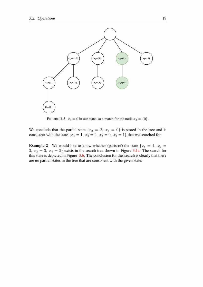
FIGURE 3.5: x3 = 0 in our state, so a match for the node x3 = {0}.

We conclude that the partial state {x2 = 2, x3 = 0} is stored in the tree and isconsistent with the state {x1 = 1, x2 = 2, x3 = 0, x4 = 1} that we searched for.

Example 2 We would like to know whether (parts of) the state {x1 = 1, x2 =3, x3 = 3, x4 = 3} exists in the search tree shown in Figure 3.1a. The search forthis state is depicted in Figure 3.6. The conclusion for this search is clearly that thereare no partial states in the tree that are consistent with the given state.

20 Chapter 3. Search tree

(a) x1 = 1 in our state, so no match for the nodex1 = {2, 3}.

(b) x2 = 3 in our state, so no match for the nodex2 = {1}.

(c) x2 = 3 in our state, so no match for the nodex2 = {2}.

(d) x4 = 3 in our state, so no match for the nodex4 = {0}.

FIGURE 3.6: Searching for {x1 = 1, x2 = 3, x3 = 3, x4 = 3} inthe search tree shown in Figure 3.1a.

3.2.2 InsertIdea Inserting in this search tree is relatively simple; we follow existing branchesas much as possible, and as soon as a node does not exist in a certain place in thesearch tree, we create a new sub-branch at that point. Let us now take a look at someexamples. Note that in these examples a green node represents a newly added node,whereas an orange node represents an existing node that has changed (in other words,the set of values in that node has changed).

Example 1 We would like to insert the partial state {x2 = 1, x3 = 0} in the searchtree shown in Figure 3.1a. The insert operation is shown in Figure 3.7. The partialstate {x2 = 1} was already present, and its branch is extended with a new child-node{x3 = 0}.

3.2. Operations 21

FIGURE 3.7: Inserting the partial state {x2 = 1, x3 = 0} into thesearch tree shown in Figure 3.1a.

Example 2 Suppose we would now like to add the partial state {x2 = 2, x4 = 1}to the tree that is shown in Figure 3.7. A naive way of doing this is displayed inFigure 3.8; the partial state x2 = 2 was already present,and its branch is extendedwith a new child-node x4 = {1}.

FIGURE 3.8: Inefficient insertion of {x2 = 2, x4 = 1} into the treethat is shown in Figure 3.7.

This yields, however, a tree with two (nearly) identical sub-trees: ({x2 = 1} and{x2 = 2}). The only difference between these branches is the values in their parentnode x2. This means that we are storing the same sub-trees twice, with a minordifference. It would be much more efficient to merge these overlapping sub-treesinto one by simply merging the values of the x2 nodes, as can be seen in Figure 3.9.

22 Chapter 3. Search tree

FIGURE 3.9: Efficient insertion of {x2 = 2, x4 = 1} into the treethat is shown in Figure 3.7.

This compact notation saves a lot of memory. This is especially the case when theCSP consists of many variables with large domains since this would result in manyextra branches if stored naively.

3.3 AccessWe now have a data structure that can be used to avoid duplicate searches amongstall threads. In practice, we will only need one instance of this tree to store both thesolutions and the partial states that have been covered before. However, the followingquestion naturally arises; what should the access rights of the threads on these searchtrees be? Are there any complications when we allow all threads to insert and searchin the search trees? Moreover, what happens if a thread wants to insert a new (partial)state while another thread is searching for another (partial) state?

3.3.1 OperationsSearch Since each slave thread must be able to prematurely abort a search if (a partof) the current state has been covered before, it is crucial that the slave threads haveat least search access to the tree. Otherwise, the benefits of storing previous attemptsin the search trees to avoid duplicate searches would cease to exist.

Insert Since the master thread is used as a middle man to get new tasks, it can alsobe used as a middle man for inserting a new (partial) state in the search trees. Thisapproach ensures that all states are inserted consecutively, which is crucial as we donot want to insert multiple states at the same time. Therefore, only the master threadhas insert access to the tree and the slave threads will have to signal the master threadto request insertions in the tree.

The access rights of the threads on the search trees are shown in Figure 3.10.

3.3. Access 23

FIGURE 3.10: A diagram showing the access rights of the threads tothe search tree.

3.3.2 Data RaceA common problem that may occur in a parallelized application is when multiplethreads try to access the same shared memory simultaneously, while (at least) oneof the threads is trying to modify the data stored in this memory location. Thisphenomenon is called a data race and can lead to unintended behaviour (when theoperations are executed in the wrong order, for example). In the case of the searchtrees, a data race may occur when the master thread is inserting a (partial) state intothe search tree, while a slave thread is trying to search for a (partial) state in the samebranches. Luckily, data races can be solved by making use of objects called mutexes.A mutex serves as a lock on shared memory and allows only one thread access to thismemory at a time. If a thread would like to access this shared memory, it will firstrequest to lock the corresponding mutex. If the mutex is already locked, however,the thread will be blocked until the mutex is unlocked by another thread. Once thisis the case, the thread now locks the mutex and can continue its work.

In our solver, we have one mutex for the entire search tree. Now, whenever a threadtries to read a node in a branch that is currently being processed by an insert operation(performed by the master), it will be blocked until the insert operation has finished.

24

Chapter 4

CSP specification language

In order to be able to specify CSPs in a compact manner, we designed a simplespecification language. We will first take a look at an example CSP defined in thislanguage, before covering the details of the language.

Recall that the 8-queens problem can be specified as a formal CSP as follows:

• X = {X1, . . . , Xn}, where each Xi is the column of the queen that is placedon row i of the chess board.

• For each Xi we have Di = {1, . . . , 8} (i.e. column numbers).

• C = AllDiff (X1, . . . , Xn) ∪ {j − i 6= abs(Xi −Xj) | 1 ≤ i < j ≤ n}.

In our specification language, this would be represented as follows:# Find all solutions for the N queens problem. In this case, N = 8const N = 8;

typecolumn = {0..N-1};

csp diagonalCheck(board[0..N-1] : column) beginconstraint{forall (i in [0..N-1]:forall (j in [i+1..N-1]:j - i != abs(board[i] - board[j]);

))

}end

csp main() beginsolutions all;

varboard[0..N-1] : column;

constraint{alldiff(board);diagonalCheck(board);

}end

We will use this example to explain the details of the specification language.

4.1. Constants 25

4.1 ConstantsThe first line of code is const N = 8;. As one might expect, this defines a globalconstant. Global constants are declared at the very top of the file and their scopeis the entire file, including sub-CSPs. Their names must start with a capital letter,followed by numbers or lowercase letters. Moreover, their values must be constant(either an integer, a Boolean value, or an enumeration value).

4.2 TypesThis (optional) section can be used to define types, which can be used to reuse do-mains that are used for multiple variables. Types (and therefore domains) are eithersets of integers or sets of enumerable values:

• Integers contains only integers, ranges or constants. This is present in the8 queens problem CSP: column = {0..N-1}. The type column nowrepresents the set {0, 1, . . . , N − 2, N − 1}.

• Enumeration contains strings of options that a variable can be. An exam-ple of this can be found in the implementation of the map-colouring prob-lem in this specification language (found in Appendix A.1.2). In there, wehave colour = {red, green, blue, yellow}. This is more user-friendly than having a type colour = {0, 1, 2, 3}, where each num-ber would represent a colour.

Types defined in this section can be used in all CSPs.

4.3 CSPsThe specification language supports multiple (sub-)CSPs in one file, as can be seenin the example. There must be at least one CSP, though, named main with no pa-rameters. The solver will always start by solving this CSP. All other sub-CSPs arethen only solved if there is a path between the main CSP and the given sub-CSP. Asan example, let us take a look at the following input file:

csp d(x) beginconstraint{x != 5;

}end

csp c(x) beginconstraint{x != 4;d(x);

26 Chapter 4. CSP specification language

}end

csp b(x) beginconstraint{x != 3;

}end

csp a(x) beginconstraint{x != 2;b(x);

}end

csp main() beginvarx : {1..10};

constraint{a(x);

}end

The CSP c is never solved, as there is no reference to it. The CSP d does have a ref-erence from c, but since c ixtself cannot be reached from main, d is consequentlyalso never solved, as it is only referenced in c.

A CSP declaration starts with its name and its (optional) parameters. Only the nameof the parameters is provided (including the size if a parameter is an array). Anexample of a sub CSP with parameters:

csp diagonalCheck(board[0..N-1]) beginconstraint{forall (i in [0..N-1]:

forall (j in [i+1..N-1]:j - i != abs(board[i] - board[j]);

))

}end

Aside from its heading, a (sub-)CSP also has a body. The body (may) contain threesections, each of which we will cover next.

4.3. CSPs 27

4.3.1 SolutionsThis (optional) section can be used to define the number of solutions that are re-quested. The options are solutions all, solutions single and solutionsn, for some natural number n. If no option is declared, the default option will be used,which is solutions all. Moreover, if there are only m solutions, with m < n,then the system will only show those m solutions (in other words, n is an upperbound).

4.3.2 VariablesIn this section, the user can declare the variables that are used in the constraints. Avariable declaration has one of the following forms:

• variable : type

• variable : boolean (note that {boolean} is a built-in type)

• variable : set (for example, variable : {0..N})

Moreover, a variable can also be an array. The syntax for arrays is similar to theformats above;

• variable[0..N] : type

• variable[0..N] : boolean

• variable[0..N] : set

In the case of the 8-queens problem, we find the declaration board[0..N-1] :column, which is equivalent to board[0..7] : {0..7}. Arrays of higherdimensions are also supported by separating the indices by commas. An example ofthis can be seen in the sudoku implementation (found in Appendix A.1.3):

sudoku[1..9, 1..9] : {1..9}

Note that the user is free to choose the starting and ending indices of arrays. Thisallows the user to start indexing at any non-zero value, should they want to do this.Additionally, the specification language supports declaring multiple variables of thesame type in a single line as follows:

variable1, variable2 : type

Accessing Array Elements

Apart from directly accessing elements from an array by using indices, the specifi-cation language also allows the user to access section(s) of an array. For the variablesudoku[1..9, 1..9] and board[1..8], we may do the following:

max(board) = n;

alldiff(sudoku[1, 1..9]);

sum(sudoku[1..3, 1..3]) = m;

28 Chapter 4. CSP specification language

which, respectively, correspond to:

max(board[1], board[2], board[3], board[4],board[5], board[6], board[7], board[8]) = n;

alldiff(sudoku[1,1], sudoku[1,2], sudoku[1,3],sudoku[1,4], sudoku[1,5], sudoku[1,6],sudoku[1,7], sudoku[1,8], sudoku[1,9]);

sum(sudoku[1,1], sudoku[1,2], sudoku[1,3],sudoku[2,1], sudoku[2,2], sudoku[2,3],sudoku[3,1], sudoku[3,2], sudoku[3,3]) = m;

4.3.3 ConstraintsA constraint can consist of several options:

• Binary comparison: a binary comparison of the form Expression operatorExpression, where operator∈ {=, !=, <, <=, >, >=}. An Expressioncan either be a Boolean expression, or a numeric expression. An example of abinary comparison using numeric expressions is

j - i != abs(board[i] - board[j]);

There are a few built-in mathematical functions available; abs, min, max andsum. For these functions, you can also pass ranges of variables (as discussedin Chapter 4.3.2):

sum(square[i, 0..SIZE-1]) = RESULT;

which is equivalent to:

sum(square[0,0], square[0,1],square[0,2], square[0,3]) = 34;

for i=0, SIZE=4 and RESULT=34.

• CSP call a call to a sub-CSP, including its parameters. An example that wehave seen already is alldiff(board).

• Forall statement a for-loop alike construct that allows the user to iterativelydefine (parts of) a constraint. The syntax is:

forall (iterVar in [start..end]:constraint;

)

where start and end are numeric expressions. An example of such a forallstatement can be found in the 8 queens problem:

4.4. Further Examples 29

forall (i in [0..N]:forall (j in [i+1..N]:

j - i != abs(board[i] - board[j]);)

)

which represents the set of constraints {j−i 6= abs(Xi−Xj) | 1 ≤ i < j ≤ n},where Xi = board[i-1].

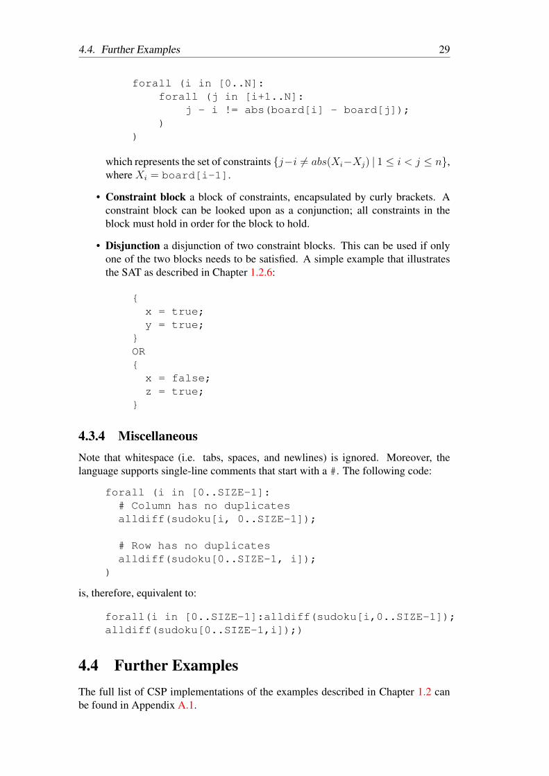
• Constraint block a block of constraints, encapsulated by curly brackets. Aconstraint block can be looked upon as a conjunction; all constraints in theblock must hold in order for the block to hold.

• Disjunction a disjunction of two constraint blocks. This can be used if onlyone of the two blocks needs to be satisfied. A simple example that illustratesthe SAT as described in Chapter 1.2.6:

{x = true;y = true;

}OR{x = false;z = true;

}

4.3.4 MiscellaneousNote that whitespace (i.e. tabs, spaces, and newlines) is ignored. Moreover, thelanguage supports single-line comments that start with a #. The following code:

forall (i in [0..SIZE-1]:# Column has no duplicatesalldiff(sudoku[i, 0..SIZE-1]);

# Row has no duplicatesalldiff(sudoku[0..SIZE-1, i]);

)

is, therefore, equivalent to:

forall(i in [0..SIZE-1]:alldiff(sudoku[i,0..SIZE-1]);alldiff(sudoku[0..SIZE-1,i]);)

4.4 Further ExamplesThe full list of CSP implementations of the examples described in Chapter 1.2 canbe found in Appendix A.1.

30

Chapter 5

Workflow

5.1 Reading and parsingTo read and parse CSP specification files, we make use of the parser generator Bi-son in combination with the lexical analyser generator Flex. Loosely speaking, Flextokenizes the input text and provides these tokens to a parser that was generated byBison. This parser determines whether the sequence of tokens is according to thespecified grammar. If this is the case then the parser returns an array of structsthat is constructed (in so-called grammar action rules) during the parsing process. Ifthe input does not follow the specified grammar, however, the parser will throw anerror and let the user know which token resulted in an error. In addition to the regularerror reporting provided by Bison, we have extended this to also show in which linenumber the incorrect token is found. This, of course, takes into account white spaceand comment lines.

On success, the parser returns a struct Program which was built while parsingthe input. This struct is a data type that contains all the data of the CSP specificationfile and we may proceed to the next step of the program, which is parsing the pro-gram arguments.

We have added support for the following run-time flags:

• -t=n: the flag -t allows the user to specify how many slave threads maybe used by the solver. Note that in the case that -t=1 is specified, then theprogram will run sequentially;

• -st=n: the flag -st allows the user to specify whether they want to use thesearch trees to store intermediate, partial states in, and n ∈ {0, 1};

• -a=n: the flag -a allows the user to specify whether they want to use arcconsistency inference, and n ∈ {0, 1};

• -n=n: the flag -n allows the user to specify whether they want to use nodeconsistency inference, and n ∈ {0, 1};

• -p=n: the flag -p allows the user to specify whether they want to solver toprint the solutions, and n ∈ {0, 1}.

Note that these program arguments may be given in any order, and if duplicatearguments exist, the last ones will be used. If some program arguments are notprovided, however, their default values will be used;

5.2. Reduced Form 31

• -t=numAvailableThreads for Linux, and -t=8 for macOS;

• -st=0, -a=0, -n=1, and -p=1 for all operating systems.

5.1.1 Setting program scopeLastly, we set the scopes in the Program accordingly. A scope is a struct thatcontains a list of all constants, sub-CSPs, variables, and parameters that can be calledor accessed at a certain location in the code. Each CSP has its own scope containingall parameters and variables that are locally declared. These parameters and vari-ables should not be accessible to other CSPs, and should, therefore, only occur in thescope of the corresponding CSP. Aside from these scopes, the Program also con-tains a global scope that contains a list of all constants and sub-CSPs defined in a file.

The next step is generating a reduced (simplified) variant of the CSP and solving thisvariant.

5.2 Reduced FormSo far, we have seen what a CSP looks like in the specification language. The actualsolver, however, does not directly solve CSPs defined in this language. Instead, itfirst translates the input into a reduced variant of the specification language. Thislanguage is a simpler version of the original language and is used as a normal formby the solver. This intermediate, reduced form is never seen by the user, and thesimplifications in this reduced form make the solving process significantly easier.

The following changes have been made in the reduced specification language (withrespect to the original language):

• There is only one (large) CSP, namely main. All CSP calls are (recursively)replaced by the constraints defined in the corresponding CSPs, and the vari-ables in these sub-CSPs are also copied into main. In order to avoid duplicatevariable names in main, we prefix all variables with the CSP identifier theywere defined and an underscore symbol (’_’). Note that underscores are notallowed in the original specification language. For example, a local variablex in sub-CSP sub is renamed into sub_x. For the solutions of the CSP, weonly print the variables defined in the original main CSP, since we are notinterested in the values for local variables and intermediate variables.

• Constants have been removed and all occurrences are simply replaced by theirvalues.

• Arrays have been removed. An array of size n is expanded into n separatevariables. For example, an array variable x[1,2] from the main CSP istranslated into main_x_1_2. Note that when a solution is printed, all vari-ables will be displayed in their original form (i.e. main_x_1_2 is printed asx[1,2]).

32 Chapter 5. Workflow

• Domain type sections have been removed and all domains (sets) are writtenexplicitly in the variable declarations.

• Domains are expanded to an array of values, rather than an array of ranges andvalues. Moreover, if there were any duplicates before, they are removed.

In the reduced format, constraints are also expanded as much as possible:

• Array ranges are expanded into n binary comparisons, where n is the numberof elements in the array range.

• All forall statements are replaced by n copies of the body, where n =end-start.

• alldiff is expanded into n binary comparisons, where n is the number ofelements in the parameter variable(s).

Example Given the implementation of the 8 queens problem in the regular speci-fication language, the reduced form variant would be as follows:csp main() beginsolutions all;

varmain_board_0 : {0,1,2,3,4,5,6,7};main_board_1 : {0,1,2,3,4,5,6,7};main_board_2 : {0,1,2,3,4,5,6,7};main_board_3 : {0,1,2,3,4,5,6,7};main_board_4 : {0,1,2,3,4,5,6,7};main_board_5 : {0,1,2,3,4,5,6,7};main_board_6 : {0,1,2,3,4,5,6,7};main_board_7 : {0,1,2,3,4,5,6,7};

constraint{main_board_0 != main_board_1;main_board_0 != main_board_2;main_board_0 != main_board_3;main_board_0 != main_board_4;main_board_0 != main_board_5;main_board_0 != main_board_6;main_board_0 != main_board_7;main_board_1 != main_board_2;main_board_1 != main_board_3;main_board_1 != main_board_4;main_board_1 != main_board_5;main_board_1 != main_board_6;main_board_1 != main_board_7;main_board_2 != main_board_3;main_board_2 != main_board_4;main_board_2 != main_board_5;main_board_2 != main_board_6;main_board_2 != main_board_7;main_board_3 != main_board_4;main_board_3 != main_board_5;main_board_3 != main_board_6;main_board_3 != main_board_7;main_board_4 != main_board_5;main_board_4 != main_board_6;main_board_4 != main_board_7;main_board_5 != main_board_6;main_board_5 != main_board_7;main_board_6 != main_board_7;((1)-(0)) != abs(((main_board_0)-(main_board_1)));((2)-(0)) != abs(((main_board_0)-(main_board_2)));

5.2. Reduced Form 33

((3)-(0)) != abs(((main_board_0)-(main_board_3)));((4)-(0)) != abs(((main_board_0)-(main_board_4)));((5)-(0)) != abs(((main_board_0)-(main_board_5)));((6)-(0)) != abs(((main_board_0)-(main_board_6)));((7)-(0)) != abs(((main_board_0)-(main_board_7)));((2)-(1)) != abs(((main_board_1)-(main_board_2)));((3)-(1)) != abs(((main_board_1)-(main_board_3)));((4)-(1)) != abs(((main_board_1)-(main_board_4)));((5)-(1)) != abs(((main_board_1)-(main_board_5)));((6)-(1)) != abs(((main_board_1)-(main_board_6)));((7)-(1)) != abs(((main_board_1)-(main_board_7)));((3)-(2)) != abs(((main_board_2)-(main_board_3)));((4)-(2)) != abs(((main_board_2)-(main_board_4)));((5)-(2)) != abs(((main_board_2)-(main_board_5)));((6)-(2)) != abs(((main_board_2)-(main_board_6)));((7)-(2)) != abs(((main_board_2)-(main_board_7)));((4)-(3)) != abs(((main_board_3)-(main_board_4)));((5)-(3)) != abs(((main_board_3)-(main_board_5)));((6)-(3)) != abs(((main_board_3)-(main_board_6)));((7)-(3)) != abs(((main_board_3)-(main_board_7)));((5)-(4)) != abs(((main_board_4)-(main_board_5)));((6)-(4)) != abs(((main_board_4)-(main_board_6)));((7)-(4)) != abs(((main_board_4)-(main_board_7)));((6)-(5)) != abs(((main_board_5)-(main_board_6)));((7)-(5)) != abs(((main_board_5)-(main_board_7)));((7)-(6)) != abs(((main_board_6)-(main_board_7)));

}

end

5.2.1 Preparing CSPBefore we can start solving the CSP main, we first need to make some preparations,as the CSP is not ready to be solved straight after having been parsed. We do this byperforming the following actions:

Setting scope We set the scope for the CSP in this step in a similar way as discussedin Chapter 5.1.1. Since the reduced specification language only consists of one CSPmain with no parameters, and constants are removed, the scope simply consists ofall the variables that are defined in main.

Infer variable types Next, we iterate over all variables and infer the type of thevariable by looking at the values in its domain. Based on these values, we assign oneof the following types to the variable: INT_TYPE, BOOL_TYPE, or ENUM_TYPE.Moreover, if a variable is of type BOOL_TYPE, we assign the domain {0, 1} to it.Note that we could also assign the enum domain {true,false} to it, but since aBOOL_TYPE is treated as an INT_TYPE, it is simply easier to assign the set {0, 1}to it.

Set assignments The following step is to look at all the constraints and checkwhether there are any assignments present, that are not part of any disjunctions, ofthe form variable = constant or constant = variable, where a con-stant value is either a Boolean value, an integer, or an enumeration value (string). Ifthis is the case, we assign this constant value to this variable and disable this con-straint such that it will not be inspected anymore in the future, to avoid unnecessarilylooking at these constraints and thereby increasing the performance.

34 Chapter 5. Workflow

Remove duplicates Since the types were removed and replaced by sets, it maybe the case that there are overlapping numbers in the set. For example, the typetType : {1..9, 7} will be translated into {1,2,3,4,5,6,7,8,9,7}, inwhich 7 occurs twice. Therefore, we must get rid of all duplicates values in thedomains of the variables to avoid (unnecessary) duplicate searches. After the removalof duplicates, the domains are simple arrays containing values (and no ranges), suchthat we can iterate over the values in domains.

Link constraints In this step, we visit all constraints. If there is a constraint inwhich a variable name occurs, we find the corresponding variable that is stored inthe scope and assign it to the variable in the constraint. We can now directly use thevariables stored in the constraints, rather than searching it in the scope every time weneed to access it.

Simplify constraints The constraints that are given in the reduced form can (some-times) be simplified. For example, in the following (reduced) constraint from the8-queens problem

((1)-(0)) != abs(((board_0)-(board_1)))

the term ((1)-(0)) can clearly be simplified to 1. Since all constraints are binarycomparisons in their core, we iterate over all these binary comparisons and checkwhether the expressions on the left-hand side and right-hand side can be simplified.If this is the case, we replace the expressions with these simplifications.

5.3 ParallelizationFor the parallelization of the solver, we use the POSIX pthreads library. We willspawn the slave threads from the master thread using pthread_create and startthe solving process on each thread separately. As mentioned in Chapter 3.3.2, we usemutexes to ensure that multiple pthreads do not cause a data race. We only havetwo mutexes; one for the search tree, and one for the array of tasks that is generatedby the master thread, which will be discussed in Chapter 5.3.2.

5.3.1 Load balancingLet us take a look at a CSP with the following variables:

vara : {1..10}b : {1..10}c : {1..1000000}

If we would like to solve this in parallel, with each thread starting at a differentvariable, we see that the threads that start solving at variables a and b (Ta and Tb,respectively) will likely be done relatively quickly compared to the thread that startssolving at variable c (Tc). Once Ta and Tb are done, they will have to wait for Tc tofinish, without being able to help spread the workload. In this case, Tc might take

5.3. Parallelization 35

a long time to terminate and the resources of Ta and Tb will go to waste, as theyare not helping Tc. Instead, we can create tasks for the slave threads to start solvingfrom, rather than entire variables. A task consists of a variable with a (sub) domainof the original variable. This approach allows multiple threads to be able to start thesolving process for the same variable, but at a different part of its original domain.This means that the load will be equally balanced amongst all available threads.

5.3.2 Master ThreadThe master thread (which is the thread that starts the program) will first create anarray of all the tasks for the slave threads, beforehand. This array is created by firstdetermining a sufficient task size taskSize such that load balancing is feasible.

int stateSpaceSize = getTotalDomainSize(mainCSP);int taskSize = (stateSpaceSize / n) / 100;

We do this by dividing the total state space size (in other words, the product of thesizes of all domains) by n, the number of threads available. This is, in its turn,divided by a modifier to ensure that there will be enough tasks to distribute amongstall threads. We found 100 to be a good modifier in practice.

Once taskSize has been determined, the solver iterates over all variables inmain. Each variable is split into multiple variables with domains of (at most) sizetaskSize. If a variable has a domain that is smaller than taskSize, it is simplyadded to the array of tasks without getting split.

As an example, let a be a variable with domain {1..10}. If taskSize=3, thearray of tasks will consist of the following four elements:

a : {1..3}a : {4..6}a : {7..9}a : {10}

Once the array of tasks has been made, we will spawn n slave pthreads and startthe solving process. We only spawn these threads if n > 1. If n = 1, we run thesequential version of the program.

5.3.3 Slave ThreadEach slave thread first creates a copy of the main CSP to make sure that the changesthat they make remain local and do not affect the global main CSP. Once this is done,the slave thread starts grabbing tasks that the master thread pre-computed. In orderto avoid multiple threads taking the same tasks, we use a mutex task_mutex tolimit access to the array of tasks. Once the slave thread is able to lock the mutex, itgrabs the next task and assigns it to a local variable. We then look for the variablein the main CSP that matches the name of the task variable and make a copy of thismatching variable. We need this copy in order to reset the CSP back to its originalstate after returning from the recursive solving procedure.

36 Chapter 5. Workflow

After we have made the copy, we look for the index of the variable in the CSP thatmatches the identifier (name) of the task variable. Once this match has been found,we replace the variable at this index with the task variable and start the solving pro-cess. Once the slave thread is done trying to find solutions for this task, we reset thevariable in the CSP back to the original variable and move onto the next task in thetask array. We continue this process until either the task array is empty (there are nomore tasks left), or until a global, atomic boolean variable isDone is set to true.This variable is set to true when the solver has found the desired number of solutions.This is only the case when solutions single or solutions n, of course.

Note that isDone is of type atomic_bool. Therefore, we can safely assign avalue to this variable and inspect the variable without explicitly using mutexes forthis, as C provides this functionality for us already.

The code for the slave threads is as follows:/// Slave thread which grabs tasks and starts solving the CSPs using those variables

as starting pointsvoid *consumer(void *arg) {

Program program = (Program)arg;

// Make a backup of the mainCSPpthread_mutex_lock(&program->mainCSP.mutex);CSP mainCSP = copyCSP(program->mainCSP);pthread_mutex_unlock(&program->mainCSP.mutex);

// Continue until either all solutions have been found, or there are no moretasks left

while (!isDone) {// If there are no more tasks left, we are donepthread_mutex_lock(&task_mutex);if (taskArrayPos == taskArraySize) {

pthread_mutex_unlock(&task_mutex);break;

}

// Select the next task as the starting variableVariable startVar = taskArray[taskArrayPos];taskArrayPos++;pthread_mutex_unlock(&task_mutex);

// Get the index of the identifier of the starting variable in the CSPint i;for (i = 0; i < mainCSP.body.variables.size; i++) {

if (strcmp(mainCSP.body.variables.vars[i]->ident, startVar->ident) == 0) {break;

}}

// Make a copy of the variable at this index and reset the state of the CSPVariable copy = copyVariable(mainCSP.body.variables.vars[i]);mainCSP.body.variables.vars[i] = startVar;mainCSP.body.variables.vars[i]->hasVal = true;mainCSP.state = makeState();mainCSP.state = initialiseState(mainCSP);

// Remove the starting variable from the list of unassigned variablesmainCSP.state->unassigned = removeVarNode(mainCSP.body.variables.vars[i],

mainCSP.state->unassigned);

// Start solving!backtrackingSearch(program, mainCSP, startVar);

// Reset the values backmainCSP.body.variables.vars[i] = copy;

5.4. Solving 37

mainCSP.body.variables.vars[i]->hasVal = false;freeState(mainCSP.state);mainCSP.state = NULL;

}

// Clean up the copy that was createdfreeCSP(mainCSP);

return NULL;}

5.4 SolvingThe actual solving part of the program is rather straightforward. We have a functioncalled solve which implements the backtracking search algorithm as shown in Al-gorithm 1. We select an unassigned variable from the CSP and start iterating over allthe values in its domain. If the user wants to use inferences such as arc consistencyand node-consistency, the solver will first perform the specified inferences. In orderto make the variables in a CSP arc consistent, we apply the AC-3 algorithm [16].To make the variables node-consistent (which is a simpler task), we iterate over allunary constraints and update the domains of the variables accordingly.

Once this is done, we check whether the CSP does not contain any variables thathave an empty domain. If this is the case, we do not even need to check whether theCSP is consistent, as there are no possible values for this variable.

Once we find a value for which the state remains consistent, we move onto the nextvariable in the CSP by recursively calling the solve function again. We continuedoing this until we are either at the base case (in which we have found a solution), oruntil we have run out of values.

The code for this function can be found below:/// Finds all solutions of a CSP using backtrackingvoid solve(Program program, CSP csp, Variable startVar, bool isFirst) {

// If sufficient solutions have been found, we are doneif (isDone) {

return;}

// If the CSP is complete (no more unassigned variables left), we have a solution.

// If the state of assigned variables already exists in the search tree, however,we simply skip this solution as it has been found by another thread before.

// Else, we print the solution and insert it into the stateif (isComplete(csp)) {

pthread_mutex_lock(&tree_mutex);if (!treeContainsState(csp.state->assigned, program->history)) {

insertState(csp.state->assigned, program->history);pthread_mutex_unlock(&tree_mutex);

// Atomic variable, so can safely incrementprogram->solNum++;

if (printSolutionsFlag) {pthread_mutex_lock(&program->print_mutex);printSolutionWrapper(csp.state->assigned, program->solNum);pthread_mutex_unlock(&program->print_mutex);

}

38 Chapter 5. Workflow

if (program->solNum == program->solTotal) {isDone = true;

}} else {

pthread_mutex_unlock(&tree_mutex);}return;

}

// If it is the first iteration, we assign the starting variable to startVar,which will be one of the tasks. Else, we simply select the first unassignedvariable

Variable var;if (isFirst && startVar != NULL) {

var = startVar;} else {

var = selectUnassignedVariable(csp);}

csp.state->assigned = addVarItem(var, csp.state->assigned);

// Iterate over all the elements in the setfor (int i = 0; i < var->decl.set->size; i++) {

// If sufficient solutions have been found, we are doneif (isDone) {

return;}

SetElement se = var->decl.set->elements[i];assignVariable(var, se);

// Make a backup of the variables and initialise the CSP’s stateVariableSection backupVariables = copyVariableSection(csp.body.variables);csp.state = initialiseState(csp);

// Use the tree to store intermediate results inif (useTreeFlag) {

pthread_mutex_lock(&tree_mutex);if (treeContainsState(csp.state->assigned, program->history)) {

pthread_mutex_unlock(&tree_mutex);resetCSP(csp, var, backupVariables);continue;

}pthread_mutex_unlock(&tree_mutex);

}

// Make CSP node-consistentif (makeNodeConsistentFlag) {

makeNodeConsistent(csp.body.variables, csp.body.constraints.start);

if (containsEmptyDomains(csp.state)) {resetCSP(csp, var, backupVariables);continue;

}}

// Make CSP arc-consistent. Uses the AC-3 algorithmif (makeArcConsistentFlag) {

makeArcConsistent(csp.body.variables, csp.body.constraints.start);

if (containsEmptyDomains(csp.state)) {resetCSP(csp, var, backupVariables);continue;

}}

// If the assignment leads to a consistent CSP, we go into recursion and tryto solve other variables

if (isConsistent(csp.state, csp.body.constraints.start)) {solve(program, csp, startVar, false);

}

5.4. Solving 39

// Use the tree to store intermediate, partial states inif (useTreeFlag) {

if (!isDone && csp.state->unassigned != NULL) {pthread_mutex_lock(&tree_mutex);if (!treeContainsState(csp.state->assigned, program->history)) {

insertState(csp.state->assigned, program->history);}pthread_mutex_unlock(&tree_mutex);

}}

// Reset the value and domain of the setresetCSP(csp, var, backupVariables);

}}

40

Chapter 6

Performance

We now take a look at the performance of the solver on the example CSPs. Forevery CSP (except the Boolean SAT problem, as this CSP was too small), we ran thesolver multiple times with different settings on a personal computer with an Intel(R)Core(TM) i9-9880H CPU @ 2.30GHz. We turned off printing the actual solutions tonot include I/O time in the timings. The used settings are shown in the tables belowand are as follows:

• n denotes the number of slave threads used by the solver

• T denotes whether the tree was used for the intermediate partial states (insteadof just using it to store the solutions in).

• A denotes whether the inference arc consistency was used.

• N denotes whether the inference node consistency was used.

The run-time was measured by making use of the timer.c/timer.h files,which store a start and stop, expressed as elapsed time since Unix Epoch. Therun-time is then calculated by subtracting these two times from each other.

6.1. 8 queens problem 41

6.1 8 queens problem

n

1 2 4 8 16

T = 0, A = 0, N = 0 0.090 0.405 0.209 0.124 0.105

T = 0, A = 0, N = 1 0.090 0.435 0.224 0.124 0.109

T = 0, A = 1, N = 0 0.091 0.751 0.402 0.227 0.190

T = 0, A = 1, N = 1 0.091 0.774 0.406 0.226 0.186

T = 1, A = 0, N = 0 0.090 0.473 0.364 0.351 0.456

T = 1, A = 0, N = 1 0.092 0.478 0.356 0.335 0.438

T = 1, A = 1, N = 0 0.091 0.602 0.395 0.363 0.483

T = 1, A = 1, N = 1 0.091 0.597 0.388 0.350 0.459

TABLE 6.1: Run-time (in seconds) for solving the 8 queens problemfrom Appendix A.1.1.

6.2 Map-colouring problem

n

1 2 4 8 16

T = 0, A = 0, N = 0 0.484 3.097 1.600 0.922 0.841

T = 0, A = 0, N = 1 0.483 0.984 0.501 0.291 0.280

T = 0, A = 1, N = 0 0.487 4.969 2.604 1.495 1.376

T = 0, A = 1, N = 1 0.488 1.374 0.708 0.413 0.381

T = 1, A = 0, N = 0 0.482 3.352 2.186 2.065 2.888

T = 1, A = 0, N = 1 0.480 1.110 0.737 0.671 0.828

T = 1, A = 1, N = 0 0.486 4.330 2.591 2.203 3.065

T = 1, A = 1, N = 1 0.487 1.335 0.770 0.608 0.723

TABLE 6.2: Run-time (in seconds) for solving the map-colouringproblem from Appendix A.1.2.

42 Chapter 6. Performance

6.3 Sudoku puzzle

n

1 2 4 8 16

T = 0, A = 0, N = 0 2.418 71.967 38.656 23.962 21.190s

T = 0, A = 0, N = 1 2.446 76.149 39.842 27.539 25.579s

T = 0, A = 1, N = 0 2.416 335.261 176.947 115.590 103.580s

T = 0, A = 1, N = 1 2.456 244.926 131.865 82.668 77.387s

T = 1, A = 0, N = 0 2.463 10.866 5.876 5.255 19.371s

T = 1, A = 0, N = 1 2.479 1.943 1.787 1.855 2.971s

T = 1, A = 1, N = 0 2.421 25.930 13.484 12.441 51.955s

T = 1, A = 1, N = 1 2.403 5.264 4.901 5.093 7.393s

TABLE 6.3: Run-time (in seconds) for solving the Sudoku puzzlefrom Appendix A.1.3.

6.4 Magic square puzzle

n

1 2 4 8 16

T = 0, A = 0, N = 0 73.199 73.804 41.479 42.539 36.733s

T = 0, A = 0, N = 1 73.169 86.087 47.780 47.372 41.376s

T = 0, A = 1, N = 0 72.984 152.656 86.694 88.591 72.666s

T = 0, A = 1, N = 1 73.426 168.106 98.429 103.492 80.920s

T = 1, A = 0, N = 0 74.378 145.711 155.162 311.193 301.956s

T = 1, A = 0, N = 1 73.161 154.292 151.786 311.955 302.320s

T = 1, A = 1, N = 0 73.015 205.445 156.898 320.637 320.181s

T = 1, A = 1, N = 1 75.301 221.518 165.780 322.486 322.039s

TABLE 6.4: Run-time (in seconds) for solving the magic square puz-zle from Appendix A.1.4.

6.5. Crypt-arithmetic puzzle 43

6.5 Crypt-arithmetic puzzle

n

1 2 4 8 16

T = 0, A = 0, N = 0 0.647 8.337 4.340 2.405 2.278s

T = 0, A = 0, N = 1 0.647 8.444 4.257 2.329 2.257s

T = 0, A = 1, N = 0 0.646 0.789 0.409 0.217 0.216s

T = 0, A = 1, N = 1 0.651 0.622 0.322 0.174 0.167s

T = 1, A = 0, N = 0 0.646 10.185 7.868 7.847 10.635s

T = 1, A = 0, N = 1 0.646 10.567 8.667 15.167 11.293s

T = 1, A = 1, N = 0 0.647 0.757 0.399 0.231 0.220s

T = 1, A = 1, N = 1 0.654 0.611 0.318 0.181 0.174s

TABLE 6.5: Run-time (in seconds) for solving the crypt-arithmeticpuzzle from Appendix A.1.5.

6.6 Pythagorean triples (extra)

n

1 2 4 8 16

T = 0, A = 0, N = 0 2.595 3.627 1.867 1.016 0.884s

T = 0, A = 0, N = 1 2.584 3.640 1.854 1.006 0.895s

T = 0, A = 1, N = 0 2.593 1.487 0.743 0.420 0.371s

T = 0, A = 1, N = 1 2.600 1.491 0.749 0.405 0.375s

T = 1, A = 0, N = 0 2.590 5.812 6.465 6.608 7.060s

T = 1, A = 0, N = 1 2.623 5.823 6.491 6.614 7.231s

T = 1, A = 1, N = 0 2.600 1.917 1.719 1.879 2.215s

T = 1, A = 1, N = 1 2.607 1.944 1.661 1.880 2.198s

TABLE 6.6: Run-time (in seconds) for finding all Pythagorean triplesa, b, c such that a2 + b2 = c2 with a, b, c ∈ {1, . . . , 100}, from Ap-pendix A.1.7 (but the domains of a, b, c : {1, . . . , 100} in this case).

44 Chapter 6. Performance

n

1 2 4 8 16

T = 0, A = 0, N = 0 53.540 70.236 35.542 19.598 18.632s

T = 0, A = 0, N = 1 53.568 70.309 35.948 20.516 19.173s

T = 0, A = 1, N = 0 53.713 27.890 14.169 8.215 7.250s

T = 0, A = 1, N = 1 53.867 27.313 13.874 7.921 6.550s

T = 1, A = 0, N = 0 53.855 183.501 165.553 178.496 187.053s

T = 1, A = 0, N = 1 53.645 183.076 171.349 180.851 185.382s

T = 1, A = 1, N = 0 53.497 43.456 44.963 46.592 48.839s

T = 1, A = 1, N = 1 52.967 43.461 44.998 47.807 49.054s

TABLE 6.7: Run-time (in seconds) for finding all Pythagorean triplesa, b, c such that a2 + b2 = c2 with a, b, c ∈ {1, . . . , 250}, from Ap-

pendix A.1.7.

6.7 EvaluationBased on the tables shown above in Chapter 6, we can construct the following table:

n T A N Total speed up

8 queens problem 16 0 0 0 0.86

Map-colouring problem 16 0 0 1 1.72

Sudoku puzzle 4 1 0 1 1.39

Magic square puzzle 16 0 0 0 1.99

Crypt-arithmetic puzzle 16 0 1 1 3.89

Pythagorean Triples {1,. . . ,100} 16 0 1 0 6.98

Pythagorean Triples {1,. . . ,250} 16 0 1 1 8.22

TABLE 6.8: Solver settings with the largest speed-ups for each CSPand the total speed up, compared to 1 thread.

In Table 6.8, we see that the run-time for nearly all CSPs already improved for 4threads on the best settings! The only exception to this rule is the 8 queens problem,but this is expected as this CSP has a small number of variables, a small domain, andvery “basic" constraints that are easily satisfied. Moreover, we observe that nearlyall CSPs had the fastest run-time at 16 threads, which is the number of threads thatour CPU has. We did not have access to servers with more threads to test whetherthe performance would have improved even more, unfortunately.

6.7. Evaluation 45

Additionally, it has come to our attention that the majority of these optimal settingsmake use of node consistency. This was also expected, given that most constraintsin the reduced form are binary constraints. This means that as soon as a variable isassigned a value, this binary constraint turns into a unary constraint, and since mostvariables occur in multiple of these (originally) binary constraints, making the CSPnode consistent yields in much smaller domains for many variables.

Similarly, we see that arc consistency only had a positive influence on the CSPs thathad constraints that involved three (or more) variables. As soon as one variable isassigned a value, these constraints are turned into binary constraints, which are theconstraints that can highly benefit from becoming arc consistent. The reason whythis is not the case for constraints that are “originally" binary constraints is simplythat the probability of one of the variables getting assigned a value (and thereforereducing the constraint to a unary constraint) is much higher.

Lastly, we see that using the search tree to store intermediate partial states loweredthe performance for most CSPs. This can be explained by the fact that most of theexample CSPs do not contain many variables with large domains. In these cases,searching in (and inserting into) the search tree is not worth the overhead causedby these operations, as the height of the tree is simply not that significant. For theSudoku puzzle, however, we see that using the search trees did in fact improve theperformance (which also happened to be the only option that leads to an improve-ment). This makes sense, as a Sudoku puzzle 9 × 9 = 81 variables, each with adomain of {1, . . . , 9}.

In short, we can conclude that the solver benefited from the parallelization and,in some cases, also benefited from the usage of the search trees on larger CSPs (suchas the Sudoku puzzle). The real performance gains can be seen in the larger, morecomplex CSPs, such as the crypt-arithmetic puzzle and the two Pythagorean triplesCSPs (with domains {1, . . . , 100} and {1, . . . , 250}, respectively).

46

Chapter 7

Conclusion

The goal of this bachelor thesis was to write an efficient, multi-core solver for Con-straint Satisfaction Problems (CSPs). Solving CSPs is still a relevant task to this day,and having a solver that can efficiently run on commodity hardware can be useful inseveral fields (like computer science, artificial intelligence, economics, operationalresearch, mathematics, etc.).

As we have seen in Chapter 6.7, our solver is able to solve relatively large CSPsquite quickly. We ran the solver on the example CSPs in Appendix A.1 with differ-ent options. We saw that for nearly all CSPs, there was a configuration of optionsand threads that led to a significant speed-up compared to only using one thread withno options. We noticed that the solver already started to show improvements formost CSPs when 4 threads were assigned, which is available in the vast majorityof commodity hardware. The only exceptions to this are the relatively small CSPs,for which the overhead of initiating the parallelization resulted in slightly slower runtimes, as is expected. Moreover, we saw that assigning more threads to the solveryielded better performance for the majority of the CSPs (with an exception of themap-colouring problem, the sudoku puzzle, and the magic square puzzle).

We can therefore conclude that our solver successfully met the requirements thatwe initially had and is able to offer a speed-up for the vast majority of ConstraintSatisfaction Problems on commodity hardware.

7.1 Future workEven though the solver fulfils our requirements, there is still room for improvement.Concerning usability, the main limitation is the fact that the solver only does verybasic semantic checking on the user input. It simply assumes that the input is of thecorrect form. If this is not the case, the solver might crash. Moreover, the programcurrently consists of two separate executable files; one for translating the user inputinto the reduced form, and the second one for solving this reduced variant.

Aside from this, there are also some changes that can be made to improve the effi-ciency of the solver. Currently, we have not implemented the heuristics described inChapter 1.3.1. The solver simply picks the next available variable in its list of unas-signed variables, regardless of their properties. Implementing these heuristics maylead to significant improvement in performance.

7.1. Future work 47

Moreover, we currently make a deep copy of all variables in a CSP in the recur-sive step, whereas it is only necessary to make a copy of the variables that have beenaffected by the inferences. This implementation can lead to worse performance if theinferences hardly affect the variables since they will be reset in each iteration of thealgorithm.

Another optimization that can be made is to disable the unary and binary con-straints after having made a CSP node consistent and arc consistent, respectively.These constraints can be enabled again after we move onto the next value of thedomain of the current variable, and will likely improve the performance as someconstraints are not evaluated at all.

Lastly, as discussed in Chapter 3.3.2, we only use one mutex to lock the entirehistory tree. This is may be inefficient, however, as we only need to lock downthe branches that are being inserted, not the entire search tree. Other branches mayremain intact during an insertion. Therefore, the solver may perform better if it hada mutex on every node of the tree, rather than having just one global mutex.

48

Appendix A

Specification language examples

A.1 Input CSPs

A.1.1 8 queens problem

# Find all solutions for the N queens problem. In this case, N = 8const N = 8;

typecolumn = {0..N-1};

csp diagonalCheck(board[0..N-1] : column) beginconstraint{forall (i in [0..N-1]:forall (j in [i+1..N-1]:j - i != abs(board[i] - board[j]);

))

}end

csp main() beginsolutions all;

varboard[0..N-1] : column;

constraint{alldiff(board);diagonalCheck(board);

}end

A.1.2 Map colouring problem

# Find one solution to the map-colouring problem for the provinces of theNetherlands

typecolours = {red, green, blue, yellow};

csp main() begin# no solutions-section, showcase that this is optional

vargr, fr, dr, ov, ge, fl: colours;nh, zh, ut, ze, nb, li: colours;

constraint

A.1. Input CSPs 49

{# Groningen’s neighboursgr != fr; gr != dr;

# Friesland’s neighboursfr != gr; fr != dr; fr != ov; fr != fl; fr != nh;

# Drenthe’s neighboursdr != gr; dr != fr; dr != ov;

# Overijssel’s neighboursov != dr; ov != fl; ov != ge;

# Flevoland’s neighboursfl != fr; fl != ov; fl != ge; fl != ut; fl != nh;

# Noord-Holland’s neighboursnh != fr; nh != fl; nh != ut; nh != zh;

# Gelderland’s neighboursge != ov; ge != fl; ge != ut; ge != nb; ge != li;

# Utrecht’s neighboursut != fl; ut != ge; ut != nb; ut != zh; ut != nh;

# Zuid-Holland’s neighbourszh != nh; zh != ut; zh != ge; zh != nb; zh != ze;

# Zeeland’s neighboursze != zh; ze != nb;

# Noord-Brabant’s neighboursnb != ze; nb != zh; nb != ge; nb != li;

# Limburg’s neighboursli != nb; li != ge;

}end

A.1.3 Sudoku puzzle

# Find all solutions for a given sudoku

const SIZE = 9;const BLOCKSIZE = 3;

typesType = {1..SIZE};

csp blockCheck (sudoku[0..SIZE-1, 0..SIZE-1] : sType) beginconstraint{forall (j in [0..BLOCKSIZE-1]:forall (k in [0..BLOCKSIZE-1]:alldiff(sudoku[3*j, 3*k], sudoku[3*j, 3*k+1],sudoku[3*j, 3*k+2], sudoku[3*j+1, 3*k],sudoku[3*j+1, 3*k+1], sudoku[3*j+1, 3*k+2],sudoku[3*j+2, 3*k], sudoku[3*j+2, 3*k+1],sudoku[3*j+2, 3*k+2]

);)

)}

end

csp main() beginsolutions all;

50 Appendix A. Specification language examples

varsudoku[0..SIZE-1, 0..SIZE-1] : sType;

constraint{sudoku[0,1] = 3; sudoku[0,2] = 4; sudoku[0,3] = 1;sudoku[0,5] = 5; sudoku[0,6] = 6; sudoku[0,8] = 9;

sudoku[1,1] = 9; sudoku[1,3] = 6; sudoku[1,4] = 3;sudoku[1,5] = 2; sudoku[1,8] = 1;

sudoku[2,0] = 1; sudoku[2,1] = 6; sudoku[2,2] = 5;sudoku[2,3] = 4; sudoku[2,5] = 9; sudoku[2,7] = 2;sudoku[2,8] = 3;

sudoku[3,1] = 8; sudoku[3,3] = 5; sudoku[3,4] = 1;sudoku[3,5] = 6;

sudoku[4,2] = 3; sudoku[4,3] = 8; sudoku[4,4] = 9;sudoku[4,7] = 6; sudoku[4,8] = 5;

sudoku[5,0] = 9; sudoku[5,1] = 5; sudoku[5,3] = 3;sudoku[5,5] = 7;

sudoku[6,8] = 6;

sudoku[7,1] = 4; sudoku[7,5] = 1;

sudoku[8,2] = 1; sudoku[8,4] = 5; sudoku[8,5] = 8;

forall (i in [0..SIZE-1]:# Column has no duplicatesalldiff(sudoku[i, 0..SIZE-1]);

# Row has no duplicatesalldiff(sudoku[0..SIZE-1, i]);

)# Blocks have no duplicatesblockCheck(sudoku);

}end

A.1.4 Magic square puzzle

# Find a solution for a 4x4 magic square whose columns, rows and diagonals have asum of 34 each

const SIZE = 4;const RESULT = 34;

typemgrid = {1..16};

csp main() beginsolutions single;

varsquare[0..SIZE-1, 0..SIZE-1] : mgrid;

constraint{alldiff(square);

forall (i in [0..SIZE-1]:sum(square[i, 0..SIZE-1]) = RESULT;sum(square[0..SIZE-1, i]) = RESULT;

)

sum(square[0,0], square[1,1], square[2,2], square[3,3]) = RESULT;

A.1. Input CSPs 51

sum(square[0,3], square[1,2], square[2,1], square[3,0]) = RESULT;}

end

A.1.5 Crypt-arithmetic puzzle

# Solves crypt-arithmetic puzzle TWO + TWO = FOUR

typeletter = {0..9};

csp checkCarry(f : letter, t : letter, o : letter, w : letter, u : letter, r :letter) begin

varc10, c100, c1000 : letter;

constraint{2*o = r + 10*c10;c10 + 2*w = u + 10*c100;c100 + 2*t = o + 10*c1000;c1000 = f;

}end

csp main() beginsolutions all;

varf, t, o, w, u, r : letter;

constraint{alldiff(f, t, o, w, u, r);f != 0;t != 0;checkCarry(f, t, o, w, u, r);

}end

A.1.6 Boolean SAT problem

# Find all the solutions for the logical expression (x and y) or (not(x) and z)

csp main() beginsolutions all;

varx, y, z : boolean;

constraint{{x = true;y = true;

}OR{x = false;z = true;

}}

end

52 Appendix A. Specification language examples

A.1.7 Pythagorean Triples

# Finds all Pythagorean triples in domain {1..N}. In this case, N = 250const N = 250;

typepType = {1..N};

csp main() beginsolutions all;

vara, b, c : pType;

constraint{a^2 + b^2 = c^2;

}

end

53

Bibliography

[1] J. Bakker. “A generic solver for Constraint Satisfaction Problems”. Gronin-gen: University of Groningen, 2015. URL: http://fse.studenttheses.ub.rug.nl/13059/.

[2] P. J. Campbell. “Gauss and the eight queens problem: A study in miniatureof the propagation of historical error”. In: Historia Mathematica 4.4 (1977),pp. 397–404. ISSN: 0315-0860. DOI: 10.1016/0315-0860(77)90076-3.

[3] J. Cohen. “Constraint Logic Programming Languages”. In: Commun. ACM33.7 (July 1990), pp. 52–68. ISSN: 0001-0782. DOI: 10.1145/79204.79209.

[4] K. D. Cooper. “Making Effective Use of Multicore Systems A Software Per-spective: The Multicore Transformation (Ubiquity Symposium)”. In: Ubiquity2014.September (Sept. 2014). DOI: 10.1145/2618407.

[5] B. Craenen. “Solving Constraint Satisfaction Problems with Evolutionary Al-gorithms”. PhD thesis. Nov. 2005.

[6] R. De Landtsheer. “Solving CSP Including a Universal Quantification”. In:Multiparadigm Programming in Mozart/Oz. Ed. by P. Van Roy. Berlin, Hei-delberg: Springer Berlin Heidelberg, 2005, pp. 200–210. ISBN: 978-3-540-31845-3.

[7] R. Dechter and J. Pearl. “Network-Based Heuristics for Constraint-SatisfactionProblems”. In: Search in Artificial Intelligence. Ed. by L. Kanal and V. Kumar.New York, NY: Springer New York, 1988, pp. 370–425. ISBN: 978-1-4613-8788-6. DOI: 10.1007/978-1-4613-8788-6_11.

[8] I. Dony and B. Le Charlier. “A Program Verification System Based on Oz”.In: Multiparadigm Programming in Mozart/Oz. Ed. by P. Van Roy. Berlin,Heidelberg: Springer Berlin Heidelberg, 2005, pp. 41–52. ISBN: 978-3-540-31845-3.

[9] A. E. Eiben et al. “Solving binary constraint satisfaction problems using evo-lutionary algorithms with an adaptive fitness function”. In: Parallel ProblemSolving from Nature — PPSN V. Ed. by A. E. Eiben et al. Berlin, Heidelberg:Springer Berlin Heidelberg, 1998, pp. 201–210. ISBN: 978-3-540-49672-4.

[10] E. C. Freuder. “A Sufficient Condition for Backtrack-Bounded Search”. In:J. ACM 32.4 (Oct. 1985), pp. 755–761. ISSN: 0004-5411. DOI: 10.1145/4221.4225.

[11] D. H. Frost and R. Dechter. “Algorithms and Heuristics for Constraint Satis-faction Problems”. AAI9811432. PhD thesis. 1997. ISBN: 0591621274.

54 Bibliography

[12] I. P. Gent et al. “A review of literature on parallel constraint solving”. In:Theory and Practice of Logic Programming 18.5-6 (2018), pp. 725–758. DOI:10.1017/S1471068418000340.

[13] J. Jaffar and M. J. Maher. “Constraint logic programming: a survey”. In: TheJournal of Logic Programming 19-20 (1994). Special Issue: Ten Years ofLogic Programming, pp. 503–581. ISSN: 0743-1066. DOI: 10.1016/0743-1066(94)90033-7.

[14] R. Kowalski. “The Early Years of Logic Programming.” In: Commun. ACM31 (Jan. 1988), pp. 38–43. DOI: 10.1145/35043.35046.

[15] V. Kumar. “Algorithms for Constraint Satisfaction Problems: A Survey”. In:A.I. Mag 13 (Oct. 1998).

[16] A. K. Mackworth. “Consistency in Networks of Relations”. In: Artif. Intell. 8(1977), pp. 99–118.

[17] P. Meseguer. “Constraint Satisfaction Problems: An Overview”. In: AI Com-mun. 2.1 (Jan. 1989), pp. 3–17. ISSN: 0921-7126.

[18] U. Montanari. “Networks of constraints: Fundamental properties and applica-tions to picture processing”. In: Inf. Sci. 7 (1974), pp. 95–132.

[19] C. C. Rolf and K. Kuchcinski. “Distributed Constraint Programming withAgents”. In: Adaptive and Intelligent Systems. Ed. by A. Bouchachia. Berlin,Heidelberg: Springer Berlin Heidelberg, 2011, pp. 320–331. ISBN: 978-3-642-23857-4.

[20] S. Russell and P. Norvig. Artificial Intelligence: A Modern Approach. 3rd.USA: Prentice Hall Press, 2009. ISBN: 0136042597. URL: https://dl.acm.org/doi/10.5555/1671238.

[21] V. A. Saraswat and M. Rinard. “Concurrent Constraint Programming”. In:Proceedings of the 17th ACM SIGPLAN-SIGACT Symposium on Principlesof Programming Languages. POPL ’90. San Francisco, California, USA: As-sociation for Computing Machinery, 1989, pp. 232–245. ISBN: 0897913434.DOI: 10.1145/96709.96733.

[22] E. P. K. Tsang. Foundations of constraint satisfaction. Computation in cog-nitive science. Academic Press, 1993, pp. I–XVIII, 1–421. ISBN: 978-0-12-701610-8.