Muli-Frequency Cable Vibration Experiments

Muli-Frequency Cable Vibration Experiments

by

Andrew Wiggins

Submitted to the Department of Ocean Engineeringin partial fulfillment of the requirements for the degree of

Master of Science in Ocean Engineering

at the

MASSACHUSETTS INSTITUTE OF TECHNOLOGY

June 2005

@ Massachusetts Institute of Technology 2005. All rights reserved.

A uthor .......... ..............Department of Ocean Engineering

May 18, 2005

Certified by ........ . .. . .-.-..-.. ..Michael S. Triantafyllou

Professor, Department of Mechanical and Ocean EngineeringThesis Supervisor

Accepted by................. .Michael S. Triantafyllou

Director of the Center for Ocean EngineeringMASSACHUSETTS INSTITUTE

OF TECHNOLOGY

SERA ES .20 *t

2

Muli-Frequency Cable Vibration Experiments

by

Andrew Wiggins

Submitted to the Department of Ocean Engineeringon May 18, 2005, in partial fulfillment of the

requirements for the degree of

Master of Science in Ocean Engineering

Abstract

A series of Multi-Frequency cable vibration experiments at Reynolds number 7600were carried out at the MIT Tow Tank using the Virtual Cable Towing Apparatus(VCTA). Motions observed in a Direct Numerical Simulation of a flexible cylinderin a shear current were imposed on the VCTA and force measurements taken. Re-sults showed a good agreement between the RMS lift coefficients of experiment andsimulation. Complex Demodulation Analysis revealed significant lift force phase mod-ulations. This analysis also showed that to a large extent the 3-dimensional behaviorof the DNS was captured by the 2-d experiment in regions of low inflow, and to alesser extent in regions of high inflow. Applications of results to future vortex inducedvibration force models are discussed.

Thesis Supervisor: Michael S. Triantafyllou

Title: Professor, Department of Mechanical and Ocean Engineering

3

4

Acknowledgments

First of all I would like to thank my sponsor for the opportunity to explore the rich

problem of cable vibrations. Secondly, I'd like to thank my supervisors Professor

Michael S. Triantafyllou and Dr. Franz. Hover. They have been exceedingly patient

with this project and have served as a veritable fountain of ideas. I'd also like to ac-

knowledge my predecessors at the tow tank who helped develop and refine the VCTA

apparatus. Without their work, this thesis would not have been possible. Lastly, I'd

like to thank fellow students Jason Dahl and Didier Lucor and my supportive parents.

5

6

Contents

Nomenclature 15

1 Introduction 17

1.1 M otivation . . . . . . . . . . . . . . . . . . . . . . . . . . . . . . . . . 17

1.2 The VIV Phenomenon . . . . . . . . . . . . . . . . . . . . . . . . . . 19

1.2.1 Stationary Cylinder . . . . . . . . . . . . . . . . . . . . . . . . 19

1.2.2 Flexible Cylinder . . . . . . . . . . . . . . . . . . . . . . . . . 20

1.2.3 A Long Flexible Cylinder in Shear Flow Conditions . . . . . . 25

1.3 Strip Theory Approach to the Shear Flow Problem . . . . . . . . . . 28

1.4 Previous Research at MIT and the VCTA Apparatus . . . . . . . . . 31

2 Preparation of Experiments 35

2.1 Experimental Matrix . . . . . . . . . . . . . . . . . . . . . . . . . . . 35

2.2 From DNS results to Experiment . . . . . . . . . . . . . . . . . . . . 36

2.2.1 Signal Concatenation . . . . . . . . . . . . . . . . . . . . . . . 38

2.3 Control Code and System Validation . . . . . . . . . . . . . . . . . . 44

3 Experimental Data Analysis 49

3.1 Properties of the Commanded motions . . . . . . . . . . . . . . . . . 49

3.1.1 The importance of lift force phase . . . . . . . . . . . . . . . . 50

3.1.2 CLV, CLA and CM . . . . . . . . .. . . . .. . . . . . . .50

3.2 CLV,CLA and CM, as a function of frequency . . . . . . . . . . . . . . 51

3.3 Fourier A nalysis . . . . . . . . . . . . . . . . . . . . . . . . . . . . . . 52

7

3.4 Complex Demodulation . . . . . . . . . . . . . . . . . . . . . . . . . . 57

3.5 The Hilbert Transform and related methods . . . . . . . . . . . . . . 59

3.6 Time Domain analysis . . . . . . . . . . . . . . . . . . . . . . . . . . 64

4 Results of Experiments 67

4.1 B ase C ases . . . . . . . . . . . . . . . . . . . . . . . . . . . . . . . . . 68

4.1.1 Previous multi-frequency studies . . . . . . . . . . . . . . . . . 68

4.1.2 Mono-Component vibrations . . . . . . . . . . . . . . . . . . . 72

4.1.3 DNS vs. Experiment for Flexible Cylinder in Uniform inflow . 76

4.2 Linear Shear Current Profile . . . . . . . . . . . . . . . . . . . . . . . 80

4.2.1 Low Inflow Test Location . . . . . . . . . . . . . . . . . . . . 81

4.2.2 High Inflow Test Location . . . . . . . . . . . . . . . . . . . . 83

4.3 Summary of Results . . . . . . . . . . . . . . . . . . . . . . . . . . . 85

4.4 Hydrodynamic Force Modeling . . . . . . . . . . . . . . . . . . . . . . 92

5 Future Work 97

8

List of Figures

1-1 Flow Separation[25] . . . . . . . . . . . . . . . . . . . . . . . . . . . . 19

1-2 Fixed Cylinder Wake Patterns at various Flow Conditions . . . . . . 21

1-3 Strouhal Number as a function of Reynold Number . . . . . . . . . . 22

1-4 Transition in Shedding Patterns . . . . . . . . . . . . . . . . . . . . . 22

1-5 Resonance of a rigid circular cylinder with vortex shedding . . . . . . 24

1-6 Gulf of Mexico Shear Profile . . . . . . . . . . . . . . . . . . . . . . . 25

1-7 Locked In Regions . . . . . . . . . . . . . . . . . . . . . . . . . . . . 26

1-8 Vortex W ake [8] . . . . . . . . . . . . . . . . . . . . . . . . . . . . . . 27

1-9 Typical Cylinder Motion History(Exponential Case) . . . . . . . . . . 28

1-10 Spatio-temporal cylinder crossflow displacement (Uniform Inflow) . . 29

1-11 Spatio-temporal cylinder crossflow displacement (Exponential Inflow) 29

1-12 CLV varying with spanwise position . . . . . . . . . . . . . . . . . . . 30

1-13 Strip Theory Approach . . . . . . . . . . . . . . . . . . . . . . . . . . 31

1-14 CLV contours for sinusoidal oscillations [9, pp. 78] . . . . . . . . . . . 32

1-15 VCTA Apparatus . . . . . . . . . . . . . . . . . . . . . . . . . . . . . 33

2-1 Mean frequency vs. span . . . . . . . . . . . . . . . . . . . . . . . . . 37

2-2 "Shift and Blend" type signal concatenation . . . . . . . . . . . . . . 39

2-3 Effect of model order on data-extension . . . . . . . . . . . . . . . . . 42

2-4 Backward and Forward Data Extension via AR Method . . . . . . . . 43

2-5 Cross-Fading of Signals . . . . . . . . . . . . . . . . . . . . . . . . . . 44

2-6 Typical Phase Loss between commanded and actual position . . . . . 45

2-7 Typical Commanded and Actual Position Spectra . . . . . . . . . . . 46

9

2-8 Typical Force Sensor Calibration . . . . . . . . . . . . . . . . . . . . 47

3-1 Effect of Number of Runs on 75% Confidence Intervals . . . . . . . . 54

3-2 Effect of Cosine Taper on 75 % Confidence Intervals . . . . . . . . . . 56

3-3 Frequency Resolution loss with windowing . . . . . . . . . . . . . . . 57

3-4 ICLI, |Y , and CLV from Complex Demodulation Analysis of a Purely

Sinusoidal Input M otion . . . . . . . . . . . . . . . . . . . . . . . . . 60

3-5 Instantantaneous Reduced Frequency of Input Motion via Hilbert Trans-

form . . . . . . . . . . . . . . . . . . . . . . . . . . . . . . . . . . . . 63

3-6 First 3 IMFs of a typical input motion . . . . . . . . . . . . . . . . . 63

3-7 EMD Hilbert Spectrum of Input Motion, Darker = higher amplitude 64

4-1 Wake Spectra as a function of frequency modulation ratio f/fe . . . 69

4-2 Near Wake States, from Nakano and Rockwell [17] . . . . . . . . . . . 70

4-3 Wake response state diagram for 1:20 beats [9] . . . . . . . . . . . . . 72

4-4 Wake response state diagram for 1:3 beats . . . . . . . . . . . . . . . 73

4-5 Gopalkrishnan CLV for A/D = .5, RE = 9500 . . . . . . . . . . . . . 74

4-6 CM0 from Port and Starboard Sensors, A/D = .5, RE = 9500 . . . . 74

4-7 |CLI, IYI, and CLV from Complex Demodulation Analysis of A/D =

.5, fr,RE = 9500 . . . . . . . . . . . . . . . . . . . . . . . . . . . . . 75

4-8 Time Series and Spectra for Uniform case, n = 120 . . . . . . . . . . 77

4-9 Uniform Case, Test Location . . . . . . . . . . . . . . . . . . . . . . . 79

4-10 Amplitude of motion and CL for top two frequencies, DNS and Exp.,

U niform Case . . . . . . . . . . . . . . . . . . . . . . . . . . . . . . . 80

4-11 CLv(t) and CLA(t) for top two frequencies, DNS and Exp., Uniform Case 81

4-12 Added Mass CM0 for the top two frequencies, DNS and Exp., Uniform

C ase . . . . . . . . . . . . . . . . . . . . . . . . . . . . . . . . . . . . 8 1

4-13 EMD Hilbert Spectrum of Y/D and CL, DNS and Exp.,Uniform Case 82

4-14 Time Series and Spectra for Linear case, Low Inflow . . . . . . . . . . 85

4-15 Linear Case, Low Inflow, Test Location . . . . . . . . . . . . . . . . . 86

10

4-16 Amplitude of motion and CL for top two frequencies, DNS and Exp.,

Linear Case, Low Inflow . . . . . . . . . . . . . . . . . . . . . . . . . 87

4-17 CLV(t) and CLA(t) for top two frequencies, DNS and Exp., Linear Case,

Low Inflow . . . . . . . . . . . . . . . . . . . . . . . . . . . . . . . . . 88

4-18 Added Mass Cmo for the top two frequencies, DNS and Exp., Linear

Case, Low Inflow . . . . . . . . . . . . . . . . . . . . . . . . . . . . . 88

4-19 Time Series and Spectra for Linear case, High Inflow . . . . . . . . . 89

4-20 Test Location, Linear Case, Low Inflow . . . . . . . . . . . . . . . . . 89

4-21 Amplitude of motion and CL for top two frequencies, DNS and Exp.,

Linear Case, High Inflow . . . . . . . . . . . . . . . . . . . . . . . . . 91

4-22 CLv(t) and CLA(t) for top two frequencies, DNS and Exp., Linear Case,

H igh Inflow . . . . . . . . . . . . . . . . . . . . . . . . . . . . . . . . 91

4-23 Added Mass CMo for the top two frequencies, DNS and Exp., Linear

Case, High Inflow . . . . . . . . . . . . . . . . . . . . . . . . . . . . . 92

4-24 EMD Hilbert Spectrum of Y/D and CL, DNS and Exp., Linear Case,

H igh Inflow . . . . . . . . . . . . . . . . . . . . . . . . . . . . . . . . 92

4-25 RMS values of Y and CL, 2 Cycle moving window, DNS and Exp.,

U niform Case . . . . . . . . . . . . . . . . . . . . . . . . . . . . . . . 95

11

12

List of Tables

4.1 Run Particulars, Uniform Case . . . . . . . . . . . . . . . . . . . . . 78

4.2 CLV and Cm at Peak Frequencies, Uniform Case . . . . . . . . . . . . 80

4.3 Run Particulars for Linear Case, Low Inflow . . . . . . . . . . . . . . 86

4.4 CLV and CM at Peak Frequencies, Linear Case, Low Inflow . . . . . . 87

4.5 Run Particulars for Linear Case,high Inflow . . . . . . . . . . . . . . 90

4.6 CLV and CM at Peak Frequencies, Linear Case, High Inflow . . . . . 90

4.7 Uniform Case, RMS values of lift and motion for a four frequency model 94

4.8 Linear Case, Low Inflow, RMS values of lift and motion for a four

frequency m odel . . . . . . . . . . . . . . . . . . . . . . . . . . . . . . 94

4.9 Linear Case, High Inflow, RMS values of lift and motion for a four

frequency m odel . . . . . . . . . . . . . . . . . . . . . . . . . . . . . . 94

13

14

Nomenclature

D Cylinder diameter

FL Lift force

Fd Drag force

fe Forcing frequency

L Cylinder length

p Fluid Density

Uexp Carriage Velocity

Ux Local Inflow Velocity in Simulation

Y Heave Position

z Spanwise Position

Phase between force and motion

V Volume of cylinder

(j) Amplitude Ratio

a Standard Deviation

CD = .5pULD Drag force coefficient

CL = .5pU ,LD Lift force coefficient

CLV Lift force coefficient in phase with velocity, defined in chapter 3

CLA Lift force coefficient in phase with acceleration, defined in chapter 3

Cm Added mass coefficient

f,= D Reduced Frequency

VT = f Reduced velocity

15

16

Chapter 1

Introduction

1.1 Motivation

The ability to accurately model the vortex-induced vibration (VIV) of structures is

of a practical interest to engineers in a variety of fields. In structures diverse as heat

exchanger tubes, chimney stacks and suspension bridges, VIV can govern fatigue life,

global loads and affect performance. Perhaps the most important cases of VIV occur

in the ocean, where vortex shedding regularly causes high frequency oscillations of

riser tubes and marine cables. Exposed to highly sheared flows, these high-aspect

ratio structures are particularly susceptible to VIV and pose unique challenges for

the engineer.

The phenomenon of VIV itself has been observed for centuries. Harnessing the

power of VIV, King David for instance would place his guitar above his bed such that

the breeze would excite the strings [1, pp. 11]. It was actually Leonardo Da Vinci

who first identified the physical mechanism behind VIV when he sketched the vortex

wake pattern he observed behind a bluff body in a river [1, pp. 11]. However, it isn't

until the early twentieth century with the work of Benard that these vibrations are

linked to vortex shedding [9, pp. 15].

The years surrounding the turn of the century was a particularly formative period

for VIV research. It was in this period that Strouhal discovered the fundamental

relation between the vortex shedding frequency, a body's characteristic diameter and

17

the free stream velocity (see Figure 1-3). A little later, while working on cylindrical

biplane spars, Theodore von Karman would discover the alternating vortex pattern

that now bears his name (see Figure 1-4).

VIV is a complex problem, where structural properties, the inflow velocity profile,

roughness, and viscosity all come into play in a fundamentally nonlinear manner.

This complexity leads to difficult experiments and very high computational costs at

the scales of interest. Progress has been made in solving the fully nonlinear problem,

both by experiment and simulation (see [14]-[13]),but for the majority of practical

applications simplifying assumptions have to be made.

One of simplifying assumptions often made is that the the flow is locally two-

dimensional and that the forces on the cylinder may be approximated by a strip

theory approach. The aim of this thesis is to see to what extent the true three-

dimensional behavior is captured in a two-dimensional approximation. To accomplish

this, experiments were conducted in the MIT Tow Tank and compared with the the

non-linear DNS studies of Didier and Karniadakis [14]. In addition, the sensitivity of

the response to Reynolds number was also examined.

This introduction continues with a discussion of the VIV response in various flow

regimes.

Chapter two describes the methodology used in these experiments.

Chapter three presents some of the novel post processing techniques used in the

study.

Chapter four summarizes the results of the experiments and offers conclusions and

recommendations for future work.

18

1.2 The VIV Phenomenon

1.2.1 Stationary Cylinder

As pointed out by Leonardo, the wake of a bluff body 1 is characterized by vortex

shedding. Unlike the potential flow solution to the flow around a cylinder, the pressure

distribution around a bluff body such as cylinder in real fluid is not fore/aft symmetric

and full pressure recovery does not take place. Consequently, there is a net drag force

on the object. Additionally, the boundary layer is no longer being forced onto the

body and detaches, forming a shear layer. On a cylinder, or around a sphere as in

Figure 1-1 the separation occurs near the widest part of the body. The exact location

of separation, like the wake pattern itself, is a function of the Reynolds number.

Figure 1-1 also clearly shows the shear layers rolling inward.

Figure 1-1: Flow Separation[25]

Figure 1-2 charts the effect of viscosity on the wake pattern behind a stationary

A "bluff body" is any body where the flow separates from a "large" potion of the surface

19

cylinder. At a Reynold number (RE) of around 40, vortices start to appear. These

are caused by the velocity gradient and instability in the wake. Above RE = 40,

the celebrated von Karman vortex street is formed. Two opposite signed vortice are

generated and convected downstream. Accompanying the von Karman street is a

periodic force on the cylinder. This is caused by the fact that induced velocities

from the vortices in the near wake alter the pressure distribution on the cylinder.

Integrating the pressure, it is found that there is both an alternating drag force and

lift force: the drag force occurring at a frequency twice that of the lift force. The

induced velocity due to near wake vortex also influences boundary layer development

and nearby vortices. More detailed descriptions of the vortex shedding process can

be found in Sarpkaya [19] and Williamson & Roshko[26].

The experiments in this study were performed at 1000 < RE < 20000, placing

them in the so-called "subcritical" regime. In this regime, the wake is fairly organized

and the frequency of shedding is surprisingly well-defined. The boundary is laminar up

till the separation point. Figure 1-3 shows that the Strouhal number is approximately

0.2 for the Reynolds number range of the experiment. Strouhal Number is defined in

Nomenclature section.

In the "transition" regime, at RE above 3x105 , the wake becomes less organized,

drag decreases and the shedding frequency becomes variable and sensitive to surface

roughness. The wake width also decreases.

Moving to RE beyond the transition region, Roshko [26] has found that the wake

returns to a fully turbulent von Karman street type wake. The drag coefficient in-

creases.

1.2.2 Flexible Cylinder

Thus far, only the case of a stationary cylinder has been considered. It isn't too much

of a stretch however to envision a case where the periodic forces due to the vortices are

sufficient to excite the structure. The problem then becomes one of fluid/structure

interaction, the velocity at the body no longer being simply the free stream velocity

but the vector sum of the free stream and the body motion.

20

Re < 5 REGIME OF UNSEPARATED FLOW

5 TO 15 < Re < 40 A FIXED PAIR OF FOPPLVORTICES IN WAKE

4O < Re < 90 AND 90 < Re < 1500 0 TWO REGIMES IN WHICH VORTEX

STREET IS LAMINAR

150 < Re < 300 TRANSITION RANGE TO TURBU-LENCE IN VORTEX

300 < Re Z 3 X 105 VORTEX STREET IS FULLYTURBULENT

3 X 105 Z Re < 3.5 X 106 ,

-LAMINAR BOUNDARY LAYER HAS UNDERGONETURBULENT TRANSITION AND WAKE ISNARROWER AND DISORGANIZED

3.5 X 106 < Re0 RE-ESTABLISHMENT OF TURBU-

LENT VORTEX STREET

Figure 1-2: Fixed Cylinder Wake Patterns at various Flow Conditions

In addition to being a function of Reynolds number, the wake pattern for the

compliant cylinder is also a function the motion amplitude and vibration frequency.

This can be seen in Figure 1-4. The abscissa of this graph is the reduced velocity, and

the ordinate is the motion amplitude divided by the diameter The "2S" of this chart

represents the same von Karman type street wake seen for the stationary cylinder.

The "2P" wake pattern however is something altogether different. The "2P" pattern

is characterized by two pairs of vortices being shed with each motion reversal. The

presence of unstable vortex shedding patterns such as "P+S" indicates that the ob-

servations of 1-4 were made from a forced vibration experiment, as vortex shedding

21

0.47

V;cc

CU

0.4

0.3

0.2

0.1

00 102 10

REYNOLDS NUMBER (UD/v)

Figure 1-3: Strouhal Number as a function of Reynold Number

1 -8

1-6

1-4

1-2

1.0

0.8

0.6

0-4

0-2

0 1 2 3 4 5 6 7 8 9 10X /D

Figure 1-4: Transition in Shedding Patterns

patterns such as "P+S" have not been observed to induce free vibration. The bounds

of stable wake patterns indicate that VIV motions for a symmetric body such as a

cylinder are self-limiting. [1, pp. 22].

Near a VRN = 5 (corresponding to a Strouhal Number of 0.2), there is a distinct

22

SMOOTH SURFACE/

-

P+S

-(P+S)2P

nCoaescence of

-ea -ae

- -S

change of shedding modes. This change of modes is one of the defining defining

features of flexible cylinder vibrations. "Lock-in", as it is known, occurs when the

vortex shedding frequency synchronizes with the frequency of the vibrating cylinder.

"Lock-in" is characterized by a wide peak in the response spectra. Oscillations, in

excess of 1.4 diameters have been observed in the lock-in region.

The classic results of Feng [1, 24] illustrate the lock-in phenomenon well. We see

that the frequency of shedding satisfies the Strouhal relation up until Vn = 5, at

which point the frequency of shedding collapses onto the natural frequency of the

structure. This collapse arises from the competition between the natural Strouhal

shedding mode and the one introduced with the body motion.

There are two distinct regions within the lock-in band of frequencies. In the lower

reduced velocity half of the lock-in region, energy from the near wake is input into

the structure, indicated by a positive value of CLV(see Nomenclature and the section

on Post processing for more explanation of CLV). The vortex shedding frequency is

lower than the natural stationary cylinder shedding frequency. The added mass is

usually larger than the potential flow value of one in this region.

As the reduced velocity is increased, a critical V,, is eventually reached. Recent

work by Krishanmoorthy [12] has shown that at this at the critical velocity the wake

is bistable and will change states almost periodically between 2S and 2P type vortex

formations over a couple of cycles. The phase between fluid force and motion will

behave in a similarly erratic manner. Above the critical reduced velocity, damping

occurs as the shedding process is driven by the structure. The added mass coefficient

is usually less than one in this region.

Experiments have shown that the shape of the motion response curve (shows below

in Figure 1-5) is determined by structural properties. The width of the lock-in band

is heavily influenced by the structural damping[15]. The peak amplitude of motion is

dependent on the structural damping and the cylinder mass ratio (see Nomenclature).

There are a number of interesting effects accompanying lock-in. Gopalkrishnan[9]

and others[15] have discovered the fluctuating and mean drag force is amplified at

lock-in. Flow visualization and other studies [15] have shown that at lock-in the wake

23

a,0a+ fuuw

10 I

a

1~75;

I-s

'a

on

ohIn

aa.'&

a 4 * i&a

G a I

VriU/f*D4

U'U

p

0a

.3

Figure 1-5: Resonance of a rigid circular cylinder with vortex shedding

becomes much more organized and the spanwise correlation of the wake increases.

One interesting side-effect of importance to our analysis is the observation by

Bishop and Hassan in 1964[25] that the critical transition frequency depends on

whether the frequency is being increased or decreasing. This hysteritic property

could have implications in our experiments where the frequency of oscillation is a

function of time.

24

1 ~ * 9 U .39w Y ii

1AW- . .PI

10

00

0

0*

0A

al

4

V q

0

M

4

01 a Whow" Wo *9 9 9

0.198

1.2.3 A Long Flexible Cylinder in Shear Flow Conditions

Up to this point the discussion has focused on nominally two-dimensional flows, where

the span of the cylinder is subjected to a uniform inflow velocity Uo. In actuality, more

often than not the inflow varies with the span and transverse position, U = f(y, z),

where y is the transverse position and z is the spanwise coordinate. This is case of

any riser in deep water waves, where the orbital velocities decay exponentially. The

shear flow profile is even more extreme is places such as the Gulf of Mexico, where the

orbital decay and the Gulf Stream Current combine to create highly sheared profiles

such as shown in Figure 1-6.

GoM-Gasel0

* Realdata0 Modified data

-200 64 Fourier modes fit

-400-

-600

-800-

0Z-1000

-1200

z-1400-

-1600-0 0.2 0.4 0.6 0.8 1 1.2

Non-dimensional infw velocity

Figure 1-6: Gulf of Mexico Shear Profile

Using the insight gained in the 2-dimensional discussion of Sections 1.2.1 and

1.2.2, one can reason that given a shear profile such as Figure 1-6, different regions of

the the cable may/must be locked in to different structural modes (see Figure 1-7).

The wake pattern and cylinder motion for such a case will be complicated. With

varying motion frequencies, it is improbable that the entire span of a long cylinder

will be correlated. Instead it is likely that correlated vortex "cells" will be shed. The

interaction of these "cells" with the body and other vortices is not-trivial and requires

a sophisticated coupling of the structure and fluid interactions[8]. Figure 1-8 shows

25

L rnx11

V 5 UrII

4UT

Figure 1-7: Locked In Regions

the vortex wake of one such simulation performed by George Karniadakis and Didier

Lucor [14] of Brown University.

The cylinder motion under sheared flow condition will be similarly complicated.

At the outset, it is unclear whether all modes that can be excited by a given shear flow

will participate simultaneously. It is probable that particular modes will dominate

and that transitions and interaction between modes will take place. Hydrodynamic

and structural damping will play an important role in the motion evolution, causing

spanwise waves to decay. Analysis shown in [14] and Chapter 3 shows that the cylinder

response is often very weakly stationary.

Performing a Direct Numerical Simulation (DNS) of a long flexible cylinder in a

shear flow, Karniadakis et al ([14]-[13]) observed very rich wake patterns and cable

motions. The hybrid shedding mode 2S+SP and vortex splitting was seen. Their

simulation also captured behavior such as the existence of standing waves, and waves

traveling along the cylinder span. Being DNS, their model did not resort to a turbu-

lence model, but was limited by computational cost/Reynolds number, as the mesh

size required to resolve all energy scales in three dimensional DNS is proportional to

26

Figure 1-8: Vortex Wake [8]

Re9 /4 [6]. Thus, the simulation was carried out at moderate Reynolds Numbers be-

tween 1000-3000 using parallel processing techniques to reduce computational time.

Recently, Karniadakis et. al. has done simulations of a flexible cylinder at an RE of

10000[6].

Figure 1-9 shows a typical motion history at a point along the cylinder span.

This particular time series is from a point mid-span of a cylinder in an exponential

inflow. The bottom velocity of the inflow is equal to 30% of the free-stream velocity.

Notice the intricate nature of the motion. The simulation of Karniadakis was able

to capture the presence of multi-frequency and beating patterns reported in full-scale

experiments[11].

Reproduced in Figure 1-10 and 1-11 are plots of the cross-flow displacement for

the whole span as a function of time. While both these cases exhibit a mixed type re-

sponse, the response to a uniform inflow 1-10 is dominated by standing wave patterns.

On the hand, the response to the exponential inflow, Figure 1-11 is distinguished by

traveling wave (chevron patterns). It is perhaps more useful to think of the cylinder

response more as a combination of standing and traveling waves than a superposition

of modes 1-7.

Figure 1-12 shows the lift in phase with velocity as a function of span for a number

of different shear profiles[14] (see Appendix A for the shear profiles of each case). As

will be described in more detail in Chapter 3, the lift in phase with velocity is an

indicator of the power flow of the system. A positive CLV value indicates that power is

27

Motion History, exp4, n = 64

0.5

0.4

0.3

0.2

0.1

-0.1

-0.2

-0.3

-0 A

-0.5

500

TV\ ~ t

1000 1500Sample(n)

Figure 1-9: Typical Cylinder Motion History(Exponential Case)

being transferred from the fluid to the structure. As one would expect, the structure

absorbs energy from the fluid at the side of the high inflow and viscous damping takes

place at the side of the low inflow.

1.3 Strip Theory Approach to the Shear Flow Prob-

lem

Despite recent advances in CFD tools, the prediction of VIV response is typically

carried out using semi-empirical programs such as Shear 7 and VIVA Array. These

programs aim to solve the structural wave equation given hydrodynamic forcing terms.

To evaluate these hydrodynamic terms, the programs usually have to rely on empirical

databases of hydrodynamic coefficients such as those compiled by Gopalkrishnan [9];

the result of forced vibration tests on rigid cylinders. Figure 1-14 is a contour plot of

hydrodynamic coefficients, like those used by these programs.

28

Ii(N/l

"Jul'~

i/vF

II

Ii I'W\ IJv~ II'SJill

\j

2000

iii

I AI J3~

i/'iV25000

Uniform-Re=2000

20001.5

1800 A

1600 4 0

0 W

100

800

600 O

400 -0.5

1550 1555 1560 1565 1570 1575tU/d

Figure 1-10: Spatio-temporal cylinder crossflow displacement (Uniform Inflow)

Exp-Case 1-3

2000

1800

1600

1400

1200

1000

800

600

400

200

0L1390

0.6

0.4

0.2

0

-0.2

-0.4

-0.6

1400 1410 1420 1430 1440 1450 1460 1470tU/d

Figure 1-11: Spatio-temporal cylinder crossflow displacement (Exponential Inflow)

29

Total CIv distrbution along the span

0.4- GoM-Casel

0.35 - Exp-Casel- Lin-Case2

0.3 - - -

0 .2 - - .--- --- ------- ---

0.15-

0.1 -

0.05-

0 - - - - - - --- -- - - -- - . - -

-0.05-

-0.1

0 200 400 600 800 1000 1200 1400 1600 1800z/d

Figure 1-12: CLV varying with spanwise position

Typically the structural problem is solved mode by mode in the frequency domain.

Figure 1-13 from [4] shows the loading for the second mode of a riser. Similar to Figure

1-12 a certain region of the riser is excited/locked-in while damping occurs everywhere

else. As the hydrodynamics coefficients are non-linear functions of amplitude and

frequency, and the motion amplitudes are functions of the hydrodynamic coefficients,

the problem must be solved iteratively. In this sense, the solution method the reflects

the true hydroelastic nature of the VIV problem.

While each of these programs employ structural models of varying sophistication,

they are all based on two key assumptions.

1. Motions in the inline direction can be neglected.

2. Fluid forces can be described locally as a non-linear oscillators

It is the validity of this second assumption that will be explored in this thesis. The

first assumption is currently being examined by Jason Dahl of the MIT Tow Tank.

30

II

T

-- ;00

second modeexciting region

second modedamping region

777

T T

i-p

0/

-p-p-F

-p

-0-F

-F

-F-p

-F00

-F-F

00

Figure 1-13: Strip Theory Approach

1.4 Previous Research at MIT and the VCTA Ap-

paratus

There has been a great deal of experimental research done in the area of VIV at MIT.

In addition to the standard run of forced and free vibration experiments [15],[5], re-

searchers in the tow tank have investigated the behavior of tapered cylinders [23],[24],

oscillating foils and various VIV suppressing devices [9].

There are two principal platforms for VIV testing in the tow tank, the Virtual

31

sheared flow profile

second modedamping region

1 .2 . ...... .... ..

00

.

0.2

0.4 A

010 0.05 0.1 0.15 0.2 0.25 0.3 0.35 0.4

nondimensional frequency

Figure 1-14: CLV contours for sinusoidal oscillations [9, pp. 78]

Cable Towing Apparatus (VCTA) and the Spring Cylinder Rig (SCR). A variation

on the original apparatus used by Gopalkrishnan [9] the VCTA is a versatile platform

for performing VIV tests. Running a real-time simulation of free cylinder vibration,

one is able to the alter the virtual structural properties of the system, achieving an

almost limitless set of test configurations. A substantial upgrade of the control code

on this apparatus was carried out by Oyvind Smogeli in 2002 [22].

The set-up of the VCTA can be seen in Figure 1-15, [15]. It consists of a linear

table and servo drive mounted on an A-frame, capable of heaving the test cylinder

at frequency up to 3 hz. The apparatus can handle test cylinders of up to 2 meters

in length. Lift and drag Force measurements are obtained through piezoelectric force

sensors. The amplifiers for these sensors as well as the motion control computer

are located on the carriage. The vertical position of the cylinder is measured by a

linear variable differential transformer (LVDT). It is this apparatus, used in the forced

vibration mode that is used to carry out the experiments in this study.

The SCR is a relatively new addition to the VIV lineup at the towtank. This

32

apparatus give us the capability to perform 2 DOF cylinder motion studies.

sSaw-motor

end plateae N

test cylinder -\

test cylindeforce transducer

Figure 1-15: VCTA Apparatus

33

34

Chapter 2

Preparation of Experiments

2.1 Experimental Matrix

The experiments consisted of a series of tests where the the multi-frequency cylinder

motion recorded by the Karniadakis et. al. [14] was imposed on the VCTA for a set

shear flow profiles. A total of nine different inflow profiles were considered. For the

linear and exponential profile cases three bottom velocites were investigated. We also

looked at the response to shear profiles such as those found in the Gulf of Mexico

(GOM), Figure 1-6.

As seen in Figure 1-9 and in the Brown group's work [8], the resulting cylinder

motion in these currents is quite complicated, comprised of a number of dominant

and subdominant frequencies. In this respect, the tests differed from the systematic

dual-frequency experiments of Gopalkrishnan[9]. The motions imposed on the VCTA

represent the "actual" motion at a single location on a flexible cylinder undergoing

VIV in all but two respects. One, the Reynolds number of the simulation was lower

than lower than typically experienced in the field. Secondly, the cylinder was con-

strained to move in cross-flow direction only. Because of this, whenever the results of

the experiment are to be compared directly to the DNS, we try to get the Reynolds

number as low as possible. By design a cylinder mounted on the VCTA can only

heave in the cross-flow direction, and thus provided a good basis for comparison.

To go from the raw data from the simulation, a number of operations had to

35

performed.

Proper frequency/amplitude scaling: As seen in the next section, scaling from

non-dimensional time to real time has very real effects on the feasibility of

carrying out experiments in the low inflow region.

Signal Blending and Concatenation: In order to maximize the effective run length

and minimize transient effects in the lift measurements, a scheme for concate-

nating and blending the motion signals had to be developed.

Motion Control: Accurate tracking of the prescribed motion was necessary for suc-

cesful experiments. To do this, a motion program was written for the VCTA

and validated.

2.2 From DNS results to Experiment

The results of the direct-numerical simulation are provided in columnar form, with

non-dimensional heave position (A/d), lift and drag coefficients given as a function

of non-dimensional time. (lift and drag coefficient are defined in the Nomeclature

secton). Non-dimensional time t' is given in a form similar to the Strouhal number.

t = max (2.1)D

where t is the dimensional time,Umax is the maximum inflow velocity and D is the

cylinder diameter.

Solving for t in 2.1 does not yield the time step needed for the experiment, instead

a local non-dimensional time t',using the local inflow velocity needs to be defined,

Since velocities for the simulation range from 0 to 1, where Umax = 1, the expression

for the non-dimensional time at location x is simply:

36

t- tU tU (2.2)D X

Ux is the local inflow velocity from the simulation, UO is the tow speed and Dexp

is the diameter of the test cylinder.

The implication of 2.2 for our tests is significant; for a set tow speed and test

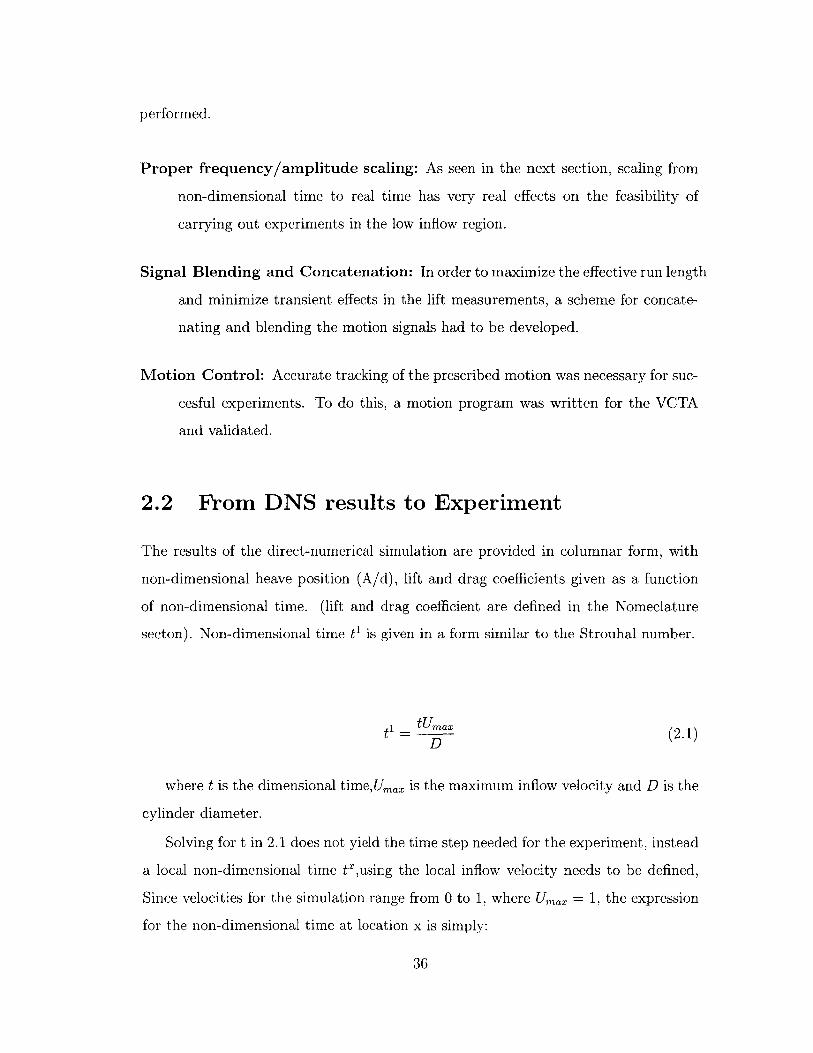
cylinder, the commanded frequency for tests in regions of low inflow has to be sig-

nificantly higher than in regions of high inflow. Logically, this makes sense since the

frequency of oscillation is largely controlled by the energetic high side. This can be

seen in Figure 2-1, where in terms of t1 , the mean excitation frequency along the span

is a relatively constant .11, with a slight decrease due to damping in the low inflow

region. Recalling 2.2, one realizes that for this shear profile where Umin = .lUma,

the frequency in Figure 2-1 would have decrease ten fold from high to low inflow for

the commanded frequency to stay the same. The upper limit of the VCTA heave

frequency is around 2 hz.

Spanwise Variation in frequency0.2

0.18 -

0.16-

30.14-E

0.12 -

C0.1 / I_ /,V/\ v

0.08-

0.06-

0.04-

0.02-

00 500 1000 1500

Spanwise Position in Diameters

Figure 2-1: Mean frequency vs. span

37

Frequency scaling issues also affect the range of Reynolds numbers that can be

acheived. Keeping the same test cylinder and test location, it follows from 2.2 that

doubling the Reynolds number requires a doubling of the commanded frequency of

motion. This means that Reynolds numbers changes are best approached by chang-

ing the cylinder diameter. Equation 2.2 poses major problems for performing high

reynolds number test at location of low inflow with the current VCTA apparatus.

Correction for the local inflow velocity also have to made to the lift and drag

coefficients.

2.2.1 Signal Concatenation

One result of the high computational cost of the DNS and the frequency scaling issue

discussed in Section 2.2 is that in real time the commanded signals are very short.

They range in length anywhere from a couple seconds for a high Reynolds number

test at a low inflow velocity location to 40 seconds in length for a moderate Reynolds

number test at a high-inflow velocity location. Given the short signal lengths and

capabilities of the MIT tank tank, we could greatly reduce the time required for

testing if we could string runs together. The only problem is that signals such as

in Figure 1-9 do not naturally flow from head to tail. To overcome this, a careful

blending technique was developed to ensure smooth transition between the end of one

signal and the beginning of the next.

The transition from rest to motion is also important for maximizing the useful

data length. The experiments showed that it takes at least a cycle for the lift signal

of a cylinder starting at rest to match that of a cylinder already in motion 1. As

the signals are already very short, it is to our advantage to minimize such transient

responses. Data length is especially crucial for spectral analysis where the data length

influences the frequency resolution.

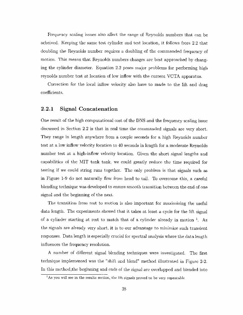
A number of different signal blending techniques were investigated. The first

technique implemented was the "shift and blend" method illustrated in Figure 2-2.

In this method,the beginning and ends of the signal are overlapped and blended into

'As you will see in the results section, the lift signals proved to be very repeatable

38

each other using a hyperbolic tangent blending window. While effective, this method

has three key disadvantages. The useful length of the parent signal is reduced, and

there is no control of the spectral content of the blending region. The method also

has an unfortunate tradeoff between the smoothness of transition and the useful data

length. If only a small portion of the signals are overlapped and the beginning and

ends of the signal are dissimilar, the transition is abrupt.

Position Blending for n 23, Usable run length = 15.9694

3-

2-

-2 -

0 10 20 340 50 60

t"m(s)

Figure 2-2: "Shift and Blend" type signal concatenation

The "shift and blend" method was eventually discarded in favor of band-limited

data extension techniques borrowed from audio and image reconstruction. Two main

classes of data-extension techiques were considered: non-iterative auto-regressive(AR)

modelling based methods[7] and iterative Papoulis-Gerchberg type algorithims[18].

The AR modelling based approach was adopted after analysis showed it to be the

most stable for a variety of gap lengths and signal phases. This method has a number

of advantages over the "shift and blend" technique. Most importantly, the original

signal is preserved in its entirety. Also, the blended region has a spectral content

similar to the parent signal.

39

Per [7] the steps needed to implement the blending are as follows:

1. Estimate a high order AR model of the signal

2. Forward Extrapolate the signal across the gap by exciting the model with zero

padded excitation

3. Backward Extrapolate the signal that succeeds the gap

4. Cross Fade

Each of the steps are discussed in the next section.

Model Estimation

The first step is to estimate a high order autoregressive model of the signal. An

autoregressive model of a process is one where the present value of the system

is the sum of P past values of X, multiplied by P filter coefficients a,, plus zero

mean white noise excitation with variance v and some forward prediction error

Et 2.3.

Xt = V + aXt_1 +...+ apXt_ + Et (2.3)

If the transfer function of the system were represented as a ratio of laplace

polynomials, it would contain only poles.

There are a number of detailed descriptions(Wu[27] and Roth[7]) of how the

filter coefficients can be easily calculated. The approach taken (known as Burg's

algorithim) is a minimization of the sum of the least squares prediction errors

under a constraint on the filter coefficients. The least squares error used is the

sum of the forward and backward and prediction errors. Matlab contains a

number of routines for the efficient calculation of these coefficients.

Nailong Wu [27] provides us another, perhaps more insightful way of looking at

the data extension technique. Rather than viewing the method as applying an

autoregressive model to a process that is not generally autoregressive, Wu proves

40

that using Burg's algorithim is equivalent to an extension by the Maximum

Entropy Method(MEM) [27, pp. 69-72]. The maximum entropy method states

of all possible data extensions the one using Burg's algoritim is the that has the

maximum entropy. Entropy is defined by equation 2.4

1

HI= f log(S(f)) df (2.4)

2

S(f) is the power spectrum and the limits of integration are from -nyquist to

+nyquist.

The determination of model order is left largely to rule of thumb. Research on

audio reconstruction by Roth et. al. indicates that the model order for data

extension should be quite high, much higher than used for spectral analysis using

Burg's method.2 . Their results showed that if the model is not high enough a

vanishing effect will occur near the center of the gap due to the minimization of

the least squares error [7, pp. 4]. We tried to reproduce this effect for one of the

DNS heave motions in Figure 2-3. Instead of the vanishing effect observed by

Roth [7], the data extension behaves erratically for lower model orders. Roth

recommends model orders of around 1000 to avoid problems. Figure 2-3 shows

that for a model order of 1000, the data extension is reasonable.

Forward Extrapolation

The AR modelling blending method is easily implement using Matlab. The

procedure consists of calculating the filter coefficients, initializing the filter with

P past values and feeding a vector of length W to the filter.

a = arburg(y,P);

2 Z = filtic(1,a,y(end-(O:(P-1))));

3 ye = filter(1,a,zeros(1,W)),Z);

2high order models are not typically used for MEM spectral analysis due to problems with linesplitting and peak shifting

41

Effect of model order on data extension14 - I I I I II I I

- Model order = 100012- 100

10-

8-

6--

0

-46--

500 1000 1500 2000 2500 3000 3500 4000 4500sample(n)

Figure 2-3: Effect of model order on data-extension

where P is the model order, y is the position and W is the length of the extension.

Backward Extrapolation The Burg algorithim is ideally suited for backward extrap-

olation since the least squared error is minimized with respect to the backwards

error in addition to the forward error. To perform backwards extrapolation the

signal is simply flipped and passed through the filter. Figure 2-4 shows the of

the forward and backward extrapolation for a typical signal.

Cross-Fading The backward and forward extrapolation are then cross-faded into each

other as shown in Figure 2-5. The gap length is chosen by the slopes at the

beginning and end of the signal and the mean frequency, such that the fit does

not produce an abrupt transition. The window used for the blending window

is defined by 2.5.

fI - (2u(n))', if u(n) 1w(n) = 2 (2.5)

1(2u(n))a, if u(n) > 1

42

Figure 2-4: Backward and Forward Data Extension via AR Method

where u(n) = (n - ns)/(ne - n,), n(s) is the starting sample, n(e) is the ending

sample, and n is the current sample. The parameter a can be varied to increase

the steepness of the window. Following the work of Roth [7], an a of 3 was used

for all blendings.

An interesting way of looking at the the effect of the blending on the response

would be to remove part of a known signal and replace it with the blended signal'.

Obviously, the the phases and amplitudes of the blended section are going to be dif-

ferent than the actual signal, but the spectra of the lift signal should be similar. This

raises the question, if the blended region are short in length compared to the overall

run, is one justified in including them as part of the signal in the spectral analy-

sis? Doing so could significantly improve the spectral resolution and/or confidence

intervals of the spectral estimates.

Once the signal has been properly concatenated, the position signal is resampled

to the desired control rate using an FFT based method, differentiated, and written

3 This is going to be tried in the next round of testing

43

S

-1

Figure 2-5: Cross-Fading of Signals

to an ASCII file to be read by the control code.

2.3 Control Code and System Validation

The control code used for the experiments is a modification of the code developed by

Smogeli [22] in 2002. To tailor the code for the needs of these particular experiments,

the capability to read a file of commanded velocities to a buffer was added. Like

previous VCTA experiments, velocity control was chosen chosen over position or

torque control in order to improve the smoothness of motion.

Velocity control does have a number of idiosyncracies that had to be addressed.

The integration of the velocity errors tends to cause the position to drift slightly

over the course of the run. For a typical run, this drift amounts to around 5% of a

diameter over 4 concatenated signals. The effect of this slowly varying drift on the

hydrodynamics however should be minimal as it is the velocity and accelation that

influence the fluid forces. The position would only come into play if there were shallow

44

*1I

7

/

I

I

- - - A 9 X-*: -M _Z* _,

I

water or free surface effects taking place. To ensure that all the tests being carried

out at roughly the same starting depth, the test cylinder is recentered regularly.

Phase loss between commanded and actual position

2.5

1.5 /

0O.5-

-1 -- commanded-2 Vactual

-2.51 I 1 2 3 4 5 6 7 8

Time(s)

Figure 2-6: Typical Phase Loss between commanded and actual position

As seen in Figure 2-6, phase loss occurs when the VCTA is run in tracking mode.

This phase loss is typically around a degree or two over the course of a run. The

phase loss is consistent with what was reported by Miller [15, pp.34] for similar

frequency forced vibrations. While this seems pretty minor, it could heavily influence

CLV if the commanded motion were used instead of the actual measured motion in

the calculation. For this reason the measured motion is always used in lift phase

calculations. Using the MEI motion exerciser, the motor is tuned with quite a bit of

velocity feed forward to try and minimize phase loss.

The overall tracking performance for a typical run can be summarized, a is the

standard deviation of the signal

45

PSD of commanded and actual position

commandedactual

1 1.2Frequency(hz)

1.4 1.6 1.8 2

Figure 2-7: Typical Commanded and Actual Position Spectra

Figure 2-7 is a comparison of the commanded and actual motion spectra as mea-

sured by the LVDT. There is good coherence at the dominant and subdominant

frequencies.

The position of the cylinder is measured both by the LVDT and a vane encoder

attached directly to the tailshaft of the servo motor. Both these devices give com-

plimentary position measurements. Using the gain for the LVDT colibration and the

motion exerciser, it was determined that conversion from meters to encoder counts is

159345 counts/meter, this factor is within 1/10 of a percent of the value used in the

Smogeli's control code header files [22, pp. 10].

The lift and drag forces are measured at the support points of the cylinder using 3-

component piezoelectric force sensors. These sensors emit a charge signal proportional

46

Coherence at top 3 Dominant Frequencies 99%

Mean position error as percent of signal o- < 1.5%

Position repeatability as percent of o- < .5%

Phase Loss over signal length ~ 1 - 2 deg

2

1.5NE

0.5~

00.2 0.4 0.6 0.8

to the shear force on the sensor. The signal is sent to the charge amplifier where it

is converted a voltage to be used either in a feedback loop or acquired. The sensors

are calibrated with the cylinder in place so that the reaction forces do not need be

considered. The calibration procedure consists of adding and removing known weights

by means of a pulley system. Figure 2-8 contains an example calibration curve. They

are typically very linear with R2 values from .99 to .999. Calibration is repeated

before and after each set of tests. Learning from Smogeli's experiments [22] steps

are taken to properly preload the force element, prevent cable flexure, and minimize

amplifier drift.

La

IiftCalibratian. m -37732NIN

10

0 L-4 -3.5 -3 -2.6 -2

Volts-1,6 -1 -0.6

Figure 2-8: Typical Force Sensor Calibration

47

48

Chapter 3

Experimental Data Analysis

3.1 Properties of the Commanded motions

When developing tools to analyze the force data and cylinder motions from the exper-

iments, two principal types of questions have to be addressed: Type 1) What is the

internal structure of the data? Type 2) What is the joint structure, or dependence

between data sets?

Recalling Figure 1-9, we see that the heave motions to be imposed on the VCTA

are intricate, often comprised of many frequencies evolving in time. A natural way of

handling Type 1 questions on irregular time series such as Figure 1-9 is to decompose

the data set into its periodic components through Fourier analysis. In the frequency

domain, one can tell which frequencies contribute prominently to the overall signal

power. Fourier analysis, however has to be applied carefully since these time series

are only weakly stationary. The motions of freely vibrating bodies such as the flexible

cylinder in the simulation are never truly constant in amplitude and frequency.[20,

pp. 395]. To determine the extent of the modulations, tools from Time/Frequency

analysis such as the Short-Time Fourier Transform (STFT),Complex Demodulation

[2, pp. 97-132] and Empirical Mode Decomposition(EMD) [10] were explored and

adopted. These methods are discussed in the following sections.

49

3.1.1 The importance of lift force phase

One of the key Type 2 questions in VIV research is the interdependence of the fluid

forcing and cylinder motion. A revealing quantity in looking at this relationship is the

phase between the the lift force and the cylinder motion. Positive #0 (force leading

motion), indicates that power (related to the sine of #0 ) is flowing from the fluid to the

body, which in turn responds by moving with a lag. The phase is a good indicator

of the vortex patterns near lock-in, where very small changes in motion frequency

can produce very large changes in phase. Lift force phase has also been shown to

be an important quantity when comparing the results of forced and free vibration

experiments [20, pp.395].

3.1.2 CLV, CLA and CMo

The phase angle is used in the typical decomposition of the lift force into an inertial

component in phase with the acceleration of the motion and a viscous/ negative

damping component in phase with the velocity of the motion. The form of lift force

is given in Equation 3.1 for a single mono-component input motion at fex:

CL(t) = (-CLocos(0o))sin(27rfet) + (CLosin(co))cos(27rfest) (3.1)

where CLo is the total measured lift coefficient, and 0 is the phase angle. The

term (-CLocos(No)) is aptly called the "lift in phase with acceleration" or CLa- It

is related to the added mass by Equation 3.2. The term in phase with the velocity,

(-CLosin(o)) is represented by the symbol CL,. These coefficients are very non-

linear functions of motion amplitude and frequency.

CM 0 = e 0 La (3.2)

27r3AYofe2x

The added mass is a non-linear function of frequency and amplitude and only

approaches its potential flow value when the frequencies of oscillation that are much

higher than the shedding frequency.

50

Since the input motion is composed of many frequencies of various amplitudes, it

is guaranteed that these coefficients will assume different values for each frequency.

If amplitude and frequency modulation occurs, the coefficients will change in time as

well. To deal with both these cases an efficient formulation of CLV, CLa, and CMo for

each component frequency was developed and is presented in the following section.

Derived in Section 3.4 are equivalent expressions for use with complex demodulation.

It is also of interest to be able to quantify the degree of similarity between the

DNS and the experimental force measurements. This is accomplished in the time

domain by means of moving windows and in the frequency domain by the coherence

function. Similar methods are used to look at the repeatability of runs and end force

correlation.

3.2 CLV,CLA and CMo as a function of frequency

The natural first step in extending the single component equations for CLV and CLA

(Equation 3.1) to ones where the force and motions are sums of sinusoids is to find

an expression for the relative phase between the time series.

Recognizing that the Fourier transforms of the motion and lift coefficient, X(f)

and CL(f) can be written in polar form, IX(f)e 27irx(f) and ICL(f)e27irCL(f), the

relative phase can be found by multiplying CL(f) by the complex conjugate of X(f),

that is

ICL,X = CL(f)X(f) = ICL(f)IIX(f)e 2xi(+cCL(f)-9x(f)) (3.3)

The lift force angle is given by Pc,x = tan-1 ( )CLX'WICL ,X

In many cases the CLA and CLV values as a function of frequency are of primary

interest. Returning to Equation 3.1, CLV can be written as

CLv(f) = CL Isir(&CL,X) - CLfXf (3-4)IX(f)I

The last form of CLV is arrived at by solving 3.3 for the second term in 3.4.

51

As a practical matter, the fast fourier transform is normally used to compute

these coefficients. To properly scale CLv(f) , Equation 3.4 needs to be divided by

the length of the fast fourier transform (FFT), N. Equation 3.5 is in the FFT ready

form.

Another practical matter involves the use smoothed estimates of 'CL,X and IX(f) |.

Smoothed estimates are made by finding the 'CL,x and |X(f)I of segments of a signal

and bin averaging. This process while seemingly beneficial tends to under predict

the CLv(f) due to the fact that the magnitude of the smoothed estimate IIcLXI is

; IX(f)IICL(f) (inequality shown in Bloomfield [2, pp.206]). Because of this, the

CLV are calculated for each segment and then averaged.

FFT ready forms of the equations for CLV(f),CLA(f) and CMo(f) are shown

below.

= 2CL(f)X(f) (3.5)N|X(f||

C~vf) C Isri~cLx)-2!NCL(f)Xf

CLA(f) = -ICLICos( cL,X) = -2RCLfXf (3.6)NIX(f)|

Cm (f) = " A(f)N (3.7)41r 3(f) 2|X(f)|DeXP

3.3 Fourier Analysis

As seen in the previous section, Fourier analysis is a valuable tool for our analysis,

allowing the computation of @CL,X simply from the cross-spectrum of the motion

and lift coefficient (Equation 3.3). Fourier analysis is also useful for quantifying

the correlation between the DNS and experiment at each frequency and in visualizing

the frequency and amplitude modulations of the signal. To estimate the modulations,

spectral analysis is applied to small segments of the signal. These Short-Time Fourier

Transforms (STFT) are calculated at a number of time steps and then plotted to

create what is known as a spectrogram.

The preliminary steps for carrying out each of these tasks are nearly identical.

52

The goal of these first steps is to create auto and cross periodiograms, or single

observations of the spectra to be estimated, for segments of the time series. The

segment lengths and data windows are chosen to achieve the required frequency and

time resolution.

To summarize, the steps taken are

1. Low-Pass Filter if necessary

2. Remove mass-inertial component of lift force

3. Separate the time series into segments

4. Detrend the time series

5. Window the series using a cosine taper

6. Zero Pad for spectral interpolation

7. compute periodogram

Time Series Segmentation: The frequency resolution of a spectral estimate, or

the ability to discern between two nearby peaks, is determined by a number of

factors. The two main factors that influence the resolution, fe, are the length

of the time series, N and the sampling rate, fe, f, = f/N is the upper bound

of the resolution. Because the sampling rate is set by the experimental set-up

(typically 250hz) or by the time resolution of the DNS, the frequency resolution

is tuned with the data length. Other operations such as windowing and bin

averaging tend to reduce frequency resolution. In cases like the power spectrum

of the lift or motion, where the regularity between segments of the signal is of

interest, the segment length is typically set fairly large, so as to get the non-

dimensional frequency resolution below .015. Examination of a number spectra

obtained by using the maximum available data length has shown that this is

sufficient to resolve almost all of the dominant frequencies in the DNS. In order

to obtain the best estimate of the underlying spectrum, the run length isn't

53

increased to its maximum. Increasing data length will no have no effect on the

confidence intervals for the spectra, because a long record only provides a single

observed value of the spectra. It is for this reason that repeat runs are also

performed. This can be clearly seen in Figure 3-1. As expected, the confidence

in the power spectrum estimate increases with the number of runs/number

of segments. In order to maximize the number of segments, they are chosen

such that they overlap(Welch's method). For details on how the approximate

confidence intervals shown in Figure 3-1 are calculated and the assumptions

involved, please see Bloomfield [2].

The effect of the number of tests on spectrum 75% confidence intervals, segment length = 1024 pt, 3 segments/run

1.8-

1.6-

+

1.2 - + + + + +

0.8- + + + + + + + + + + + + + +

0 2 6 8 10 12 14 16Number of Runs Performed

Figure 3-1: Effect of Number of Runs on 75% Confidence Intervals

The factors governing the segment length choices for the spectrogram are some-

what different from those influencing spectrum estimates. In the spectrogram

the aim is to be able to show the evolution of the frequency and amplitude

with time. This requires the data segments be chosen short enough to show

the changes in time, and long enough to resolve the frequencies of interest. A

good to think of this trade off between time and frequency resolution is to think

54

of a dirac function. A dirac function in the time domain is perfectly localized,

yet in the frequency domain spans all frequencies. Conversely, a dirac in the

frequency domain spans all time. With the spectrogram = ISTFT1.2 1, local-

ization in time and frequency is not possible and a compromise has to be made.

However, with proper segment length choice, it can yield results similar to the

methods such Wigner-Ville transform and wavelets without some of their draw-

backs. Experiments showed that a segment length of 2 cycles was sufficient to

capture the general behavior of the signal. This segment length corresponds

to a non-dimensional frequency resolution of around .04 or better. Because

of the close proximity of dominant frequencies in VIV, this but enough to re-

solve everything of interest, but is good enough to notice trends in the mean

frequency. The variation of the mean frequency displayed in the the Results

section and the Appendices was calculated using this method.

Effect of Windowing A signal of finite duration can be viewed as the multiplication

of an infinite time series by a rectangular window. In the frequency domain this

corresponds to a convolution of the fourier transform of the boxcar (a sinc) with

the true spectrum. This convolution produces spurious sidelobes that can be

misinterpreted. One of the most common ways of reducing these sidelobes is to

multiply the signal by something more periodic than the boxcar. Data windows

that are variations on a cosine bell are often used.

The windowing process also introduces less desirable effects. As can be seen

in the curve for the Hanning window in Figure 3-3, the peaks of the power

spectrum for the windowed time series are broader than for the nonwindowed

spectrum and the amplitude has been reduced. It can also be shown that the

variance of the estimate increases when windows are used [2]. This increase

shown in Figure 3-2 is fairly minor though, as the confidence intervals are more

heavily influenced by the number of segments. Due to the need to preserve

high frequency resolution, a 20% cosine taper was chosen. The 20 % refers to

'this is simply the power spectrum, a STFT is the Fourier transform of the signal after it hasbeen windowed to leave only the segment of interest

55

the total percentage of the segment that is tapered. On a 20 % cosine taper

window, the first and last 10 % is tapered. The peak of the untapered spectrum

in Figure 3-3 is matched almost perfectly by the one using the 20 % taper, we

can also see that some of the side lobes in the low frequency range are reduced.

The effect of tapering on Confidence intervals, given a set number of segments1.4

1.3- + + +

0.8- + +

0. 1 02 0.3 0.4 0.5 0.6 0.7 0.8 0.9Percent of taper, p =I is a hanning window

Figure 3-2: Effect of Cosine Taper on 75 % Confidence Intervals

Once the time series have been segmented, detrended and windowed, the pe-

riodograms are calculated. This calculation is usually carried out with the FFT,

making sure to properly normalize by the power of the of the data window.

If CLv or Cm, are to be calculated Equations 3.7,3.7,3.7 are used. As described

earlier, the values are first calculated and then averaged.

If power spectral density estimates are to be made, the periodograms are bin

averaged, made one sided and scaled by the sampling frequency. The amplitudes of

motion at the dominant frequencies are often recorded.

In the case of the periodograms used for the spectrogram, they are left alone and

plotted vs. time. To find the approximate variance in frequency, the mean frequencies

at each time step are found from the spectral moments.

56

Effect of taper length on one-sided spectrum estimate

No Taper-. 20% Taper

o Hanning

5 -

00

00

0- 0 a0

0 0 00 0

0 0

0 000

00

1.1 1.15 1.2 1.25 1.3 1.35 104 1.45 1.5 1.5Commanded Frequency (hz)

Figure 3-3: Frequency Resolution loss with windowing

3.4 Complex Demodulation

An alternate, equally valid approach to analyzing the force and motion data is to view

the signals as being composed of sinusoids of form 3.8. Unlike in Fourier analysis,

where the amplitude and phase of a given harmonic are constant, the amplitude and

phase in 3.8 are allowed to change slowly over time. This type of decomposition is

well-suited for the non-linear, history dependent nature of free vibrations [20]. As

was shown by Krishnamoorthy [12], even at the critical lock-in frequency, where the

wake structure transitions from 2S to 2P, the lift force phase oscillates and doesn't

change abruptly. Much can be learned from this approach, even when it fails. Qual-

itative knowledge that the phase isn't slowly varying, may may indicate a change in

frequency, or other phenomena. This type of an analysis can help describe features

of the response that may be missed by harmonic analysis, and can be used to better

interpret the results from harmonic analysis.

The goal of complex demodulation[2] is to extract approximations for R(t) and

#(t). This is accomplished by forming the series 3.9 by multiplying x(t) by a complex

57

sinusoid of frequency fO, the frequency of interest. This demodulation acts to zero the

frequency scale to fO. As can be seen in Equation 3.9 this creates a term from which

R(t) and 0(t) can be extracted. The process also introduces a complex sinusoid of

frequency -2f0 with varying phase. R(t)is simply the twice the modulus of the first

term, and 0(t) is the argument(Equation 3.10). The second term has to be filtered

out.

The main problem in complex demodulation is then one of filtering. In the case

of a sum of sinusoids with varying phase and amplitude in the presence of noise,

the filter has to carefully designed such that it rejects noise and sinusoids of other

frequencies(all shifted by -f0 in the demodulation). The filter used in the analysis is a

5th order low pass Butterworth filter with a cutoff frequency set at half the frequency

separation between dominant frequencies. The filter is implemented using the acausal

function filtfilt in Matlab to ensure zero phase. The use of filtfilt is equivalent to two

passes of the filter and doubles the order.

One of the most revealing applications of complex demodulation is in estimating

the time varying relative phase between force and motion. To do this, one demod-

ulates both the force and motion signal at the same frequency and computes the

difference of #CL(t) and #y(t). Care must be tken to properly unwrap the phase.

Once the relative phase is computed, Equations 3.1 and 3.2 can be applied to find the

lift in phase with velocity and added mass using the slowly varying lift amplitude.

The frequencies on which to demodulate are usually chosen from the peaks of the in-

put motion power spectrum. In these experiments the top four dominant frequencies

are analyzed. Figure 3-4 is the complex demodulation of a mono-component fixed

vibration experiment. As expected the magnitude of the motion is constant, being a

pure sinusoid, while the ICLI and CLV from the relative phase, varies over the course

of the run. Another comparison possible with complex demodulation is the relation

between the time varying amplitudes of the lift and motion. In strip theory these

should be close to linearly related for constant f, as the velocity and acceleration are

functions of R(t). However, as will be seen in the next section, this is often not the

case for the simulation.

58

Complex demodulation is closely related to the power spectrum. In a sense it is

a type of local harmonic analysis that sacrifices some frequency resolution for time

resolution. The relation between the value of R(t)(fO) and a power spectrum at

the same frequency is given in Equation 3.13. It can be shown [2] that this power

spectrum is of the same type as one produced by bin averaging. The variables a in

the denominator are the coefficients of the low pass filter.

x(t) = R(t)cos(27r(fo(t) + #(t))) = 0.5R(t) (e 2 i(fot+O(t)) + e-2i(fot+O(t))) (3.8)

y(t) = x(t)e-2"i(fot) = 0.5R(t)e2riO(t) + 0.5e-2i(2fot+O(t)) (3.9)

z(t) = O.5R(t)e27iO(t) = u(t) + iv(t) (3.10)

R(t) = 2 u(t)2 + v(t)2 (3.11)

#(t) tan-1(v(t)/u(t)) (3.12)

SX (f0) = Rt(f) 2 (3.13)N E a2

3.5 The Hilbert Transform and related methods

Very often when the time series are demodulated, a linear trend in the time varying

phase is present. Following Equation 3.8 this trend can be interpreted as a shift

in frequency. It also indicates that the frequency chosen for demodulation is not

dominant for the whole stretch of data, even though it may represent a peak in

the power spectrum. To better understand these frequency changes, time frequency

59

Complex Demodulation of Y and CL at Fr = .175, CLV computed from relative phase

2-

- Position (cm)CL

1.5 - -- C

0.5-

10 15 20 25 30time(s)

Figure 3-4: lCLl, IYI, and CLV from Complex Demodulation Analysis of a PurelySinusoidal Input Motion

tools such as the spectrogram were investigated. However, as mentioned before, the

spectrogram is not without it's limitations. To try overcome some of these limitations,

another relatively new class methods based on the Hilbert Transform was explored.

These tools can provide a very rough estimate of the instantaneous frequencies (IF)

for a multi-component signal. These too have their own severe limitations, but it is

hoped that in conjunction with other methods discussed, we may shed light on the

frequency variations in the data.

The instantaneous frequency for a mono-component signal is most often found

from the Hilbert transform. Recalling Equation 3.8, we observe that a real signal

such as a sum of sinusoids consists of both positive and negative frequencies, and

that the information contained in the negative frequencies is redundant. The Hilbert

transform is used to construct a version of the signal that contains only positive

frequencies, and maintains the signal power. One of the main advantages of doing

this is that the average frequency of the signal becomes positive.

60

Equation 3.15 shows the method in which the analytic signal, z(t) is created from

x(t). To ensure that z(t) contains only positive frequencies, the imaginary part of this

signal has to be the Hilbert transform of x(t), given in Equation 3.14. Calculation

of the Hilbert transform is straightforward and can be carried out by the function

Hilbert.m in Matlab.2 . It consists of taking the Fourier transform of x(t), multiplying

the transform X(f) by -i for negative frequencies, +i for positive frequencies, and

taking the inverse transform. For more information on the Hilbert Transform, see

Time Frequency Signal Analysis by Boualem Boashash [3].

H(x(t)) = F-'f{(-isgn(f))Ftf (x(t)} (3.14)

z(t) = x(t) + iH(x(t)) = a(t)eO(t) (3.15)

1*fi(t) = -#(t) (3.16)

2 g

To find the instantaneous frequency of the signal from the analytic signal, we

write z(t) in polar form and take the derivative of the the argument. For narrow band

signals, the IF from the Hilbert transform may be interpreted as a mean frequency.

It can be shown [3, pp. 25] however, that for wider band signals or ones where

the envelope gets small, the instantaneous frequency can give erratic results such as

infinite or negative frequencies. Figure 3-5 shows the instantaneous frequency for one

the input motions. Smoothing of the signal may reduce the variability a little, but

in general the method of finding the IF from the Hilbert transform is not directly

applicable to the results from these experiments.

If, however we could decompose our signal into a sum of narrow band functions

with near constant envelopes, the Hilbert transform could give meaningful results.

One novel method of performing such a task is known as empirical mode decompo-

sition (EMD), proposed by Huang in 1998[10]. The method seeks to break a non-

2 the function Hilbert.m in Matlab returns the complete analytic signal, not just the Hilberttransform

61

stationary signal into what are known as intrinsic mode functions (IMF) using an

iterative process. The result of this process are functions that generally satisfy the

necessary conditions for finding the instantaneous frequency via the Hilbert trans-

form. The conditions on the IMF's includes properties such as no inflection points

between extrema and zero mean'. Due to the algorithmic/data-driven nature of the

solution, EMD sometimes produces modes that are not truly IMF's. Additionally,

performance quantities such as confidence intervals are difficult to estimate. Most

importantly, it must be stressed that these intrinsic modes are not physical modes

of the system the and are only loosely orthogonal. Even, so this technique has been

successfully applied to problems in a number of fields, particularly in nonlinear wave

mechanics and metereology.

Once the IMF's are found, the instantaneous frequency and amplitude can be

computed for each mode by forming analytic associates of the modes. These can be

presented in a distribution of frequency and amplitude vs. time known as the Hilbert

Spectrum. It has been shown that the decomposition can yield similar results to

wavelets but with potentially better time/frequency resolution.

The algorithm used for EMD is described below. In the literature, the process is

known as sifting for mode functions.

1. Determine the mean of the upper and lower envelopes of the signal, mi(t). This

is usually done by a cubic spline interpolation of local maxima and minima.

2. Remove mi(t) from the data, forming hi, hi(t) = x(t) - mi(t)

3. Repeats steps 1 and 2, using hi(t) as x(t) until convergence hl,(k- 1)(t) - mli,k

hik

4. Set aside hl,k, this is the first IMF

5. Subtract hl,k from x(t) and repeat steps 1-5, to findhl..,,k

6. Stop when the result of the process produces something with a nonzero mean,

or inflection points between extrema.

62

Instantaneous Reduced Frequency of Input Motion via Hilbert transform

5 10time(s

15 20 25

Figure 3-5: Instantantaneous Reduced Frequency of Input Motion via Hilbert Trans-form

First Three IMFs of a Typical Input Motion

-.........--...........-......IMFiIMF2IMF3

-

10time(s

15 20 25

Figure 3-6: First 3 IMFs of a typical input motion

63

0.5-

0.4

4)

LI. 0.3k

0.2

0.1k

0

1.5

1

0.5

0

-0.5

0

-1

-20 5I I I I I

2r

-1.5

V

EMD Hilbert Spectrum, Position, darker = higher amplitude, log scaled amplitudeA.

0.1 II1

0.2 I I~I

-d 0.3-

0.4-

0.5-

0.6 5 10 15 20 25time(s)

Figure 3-7: EMD Hilbert Spectrum of Input Motion, Darker higher amplitude

Shown in Figure 3-6 are the IMF's of an input motion signal. The input motion

signals typically can be broken down into less than 10 IMFs, of these only three

or four contain significant energy. Figure 3-7 contains the Hilbert spectrum created

from these IMFs. The ridges provide a rough estimate of the average frequency, and

amplitude as a function of time. Again, the "modes" themselves have little or no

physical meaning.

3.6 Time Domain analysis

In addition to the frequency and time/frequency methods discussed above, a number

of statistics are computed directly from the time series from each run. These can be

useful in quantifying the correlation between DNS and experiment, identifying key

events and validating experimental methods.

The workhorse of the time domain analysis is the correlation coefficient, defined

3 Interestingly, there is an ever growing number of constraints on the definition of an IMF

64

in Equation 3.17. In an inequality related to the one mentioned in Section 3.2, the

magnitude of the covariance of two signals must be less than product of the individual

signal magnitudes. The correlation coefficient provides a number between -1 and 1

that gives us information about the phase between signals. The x(t)2 term in the

denominator is the inner product of x(t) with itself, or the autocorrelation at zero

lag. To compare the magnitudes of two signals, different statistics such as RMS values

and the coherence are computed.

Gopalkrishnan[9] and others have used an equation similar to that the correlation

coefficient for calculating CLV and CLV. The "Inner Product" forms of CLV and CLA

are given in Equation 3.18. These are calculated for each run and provide a kind

of global value for these coefficients. For pure sinusoidal cases, this result of 3.18 is

equivalent to that in equation 3.1. For a beating oscillation, 3.18 may be interpreted

as the coefficients that "when applied to a sinusoidal waveform at a carrier frequency

f, and of the same RMS amplitude, yield the same RMS output power". We also

try and approximate the global CLV and CLA as a function of time using moving

windows of approximately two cycles in length. These provide a good check for the

values from complex demodulation.

CXY = O ~) (3.17)(x(t)2, y(t)2 )

CL~i = 2(CL(t), y(t))

CLvip - 2 (CL ())(3-18)(2y(t), y(t))

CLAip - 2 (C )(3-19)

The correlation statistic is also used to look at end force correlation. In previous

work this statistic has been shown to be a good indicator of three dimensionality and

lock-in (see [5]). To look at the correlation between the DNS and the experiment,

a process similar to the one used to construct a spectrogram is used. We compute

the correlation in a moving window of approximately two cycles in length. Other

65

statistics such length of time that the correlation is above a certain limit are also

calculated. In most case signals with correlation above .5 are considered correlated.

66

Chapter 4

Results of Experiments

To validate the experimental set-up, tests were first carried out using monocomponent

input motions. Tests such as these have been studied extensively by researchers at

MIT and elsewhere[9],[25],[20]. The results of these experiments compared favorably

with past results and motivated further research. The sinusoidal motions were also a

proving ground for the post processing techniques described in the previous chapter

The second set of tests consisted of imposing the motions observed on a flexible

cylinder in uniform inflow. This set of experiments was vital in establishing a basis

of comparison for the gross lift force magnitudes of the DNS and Experiment, as the

uniform inflow case did not require the time/frequency scaling described in Chapter

2.

Finally, tests were performed at various locations along the span of a cylinder in

sheared conditions. Complex demodulation analysis showed that locally, the results

from these experiments were very similar to 2-d studies done on beating cylinders by

Gopalkrishnan and others [9],[16],[21].

Having a grasp on the response of a cylinder to 2-d beating and random oscil-

lations, we could then begin to gage to what extent the actual 3-d behavior (DNS)

was captured in the 2-d experiments. This chapter will present some representative

results from the shear flow cases and discuss implications for future modeling

67

4.1 Base Cases

4.1.1 Previous multi-frequency studies

Beginning with Bishop and Hassan[25], there has been extensive work on cylinders

forced at fixed frequency. Researchers such as Sarpkaya [20], Williamson and Roshko

[25] and Gopalkrishnan[9] have mapped the cylinder forces and characteristic vortex

patterns for a wide range of motions.

Motivated by the presence of beating patterns in marine cables, this work has

been extended to include multi-frequency tests. Systematic tests by Schargel [21],

Nakano and Rockwell [16], Gopalkrishnan have distilled many of the key attributes

of the cylinder response to multi-frequency forced vibrations.

Schargel in his Master's thesis entitled "Drag Forces on a Randomly Vibrating

Cylinder in Uniform Flow", performed a series of tests based on the the pseudo-

random vibration model developed by Kim Vandiver at MIT using an electromagnetic

shaker in the water tunnel. These tests showed a distinct broadening of the response

region, both for the oscillating and mean drag coefficients. When compared to re-

sults from a mono-component tests with the same input power, Schargel observed a

decrease in the mean drag force, and increase in the fluctuating drag force on the

randomly vibrating cylinder.

Nakano and Rockwell at Lehigh University have carried out a number of test series

of interest to us. These tests were all done at relatively low Reynolds number (100),

but allow for interesting qualitative comparisons.

In the first test series,[16] they looked at the effect of frequency modulation on

the wake structure. Equation 4.1 gives the form of the input motion y(t). fe is the

nominal excitation frequency, detuned to 95% of the natural shedding frequency for

a stationary cylinder. fm is the modulating frequency and 6fe is the deviation from

the excitation frequency, set at 50% for all tests. Varying the ratio fm/fe, they found

the wake to have a very rich spectral. As seen in Figure 4-1, for rapidly frequency

modulated signals, two significant sideband spectral peaks were present. These peaks

68

correspond exactly to locations of the first harmonics of the spectrum of 4.1. 1 At

slower frequency modulations they discovered that they could excite a wake that is

periodic over a period of 2/fm . This mode does not follow directly from the input

spectrum, and is a case where the force is not entirely "in phase" with the motion. As

the modulating frequency was further decreased, the wake destabilized and a broad

peak was present. The peak amplitude of the velocity for the slowly modulating case

was less than that for the purely sinusoidal case. The interpretation of a frequency

modulated signal as a series of sinuoids, will be important when reconciling the results

of the EMD analysis and the power spectrum.

y(t) = -Yesin{27rfet + 6fe/fmsin(27rfet)} (4.1)

10

ir

1 ~f-f

' a

Figure 4-1: Wake Spectra as a function of frequency modulation ratio fm/fe

'The spectrum of a frequency modulated signal consists of a component at fe and an infinitenumber of lines at fe nfm whose amplitudes are given by Bessel functions.

69

The second test series by Nakano and Rockwell [17] examines the effect of ampli-

tude modulation on the wake pattern. Their tests showed distinct vortex shedding

regimes based on the amplitude of the oscillation and the length of the modulating

period compared to the period of excitation. Figure 4-2 shows the states of response

of the near-wake reported by Nakano and Rockwell.

0.5

0.4

0.

0.2

0

f--periodic(fe lock-in)

fa'periodic

2fm-periodic lock-in)(non-fe lock-in) [mode n I

rm-periodic(non-fe lock-in)

mode n+1 0 /_ *__ .95

I I * I'll

0 0.57 /D

1.0

Figure 4-2: Near Wake States, from Nakano and Rockwell [17]

They identified four principal response states

* fm periodic with fe lock-in: In this structure, the instantaneous phase of the

force/vortex shedding is the same for each fe cycle. Since this is the case, the

wake is also fm periodic

* fm periodic with fe nonlock-in: In this pattern, the instantaneous phase is

different from one f, cycle to the next. However the pattern repeats itself with

each envelope.

70

3

* 2fm periodic with fe nonlock-in: Like the above except that the pattern repeats

itself everyother 1/fm period

* f m periodic with f, nonlock-in (n+1): Differs from pattern two in that an extra

pair of vortices are shed with each beat packet.

The equation of amplitude modulated input motion used by Nakano and Rockwell

was y(t) = -(Y/2)[1-cos(27rfm)]sin(27fet) 2. Like in the frequency modulated set of

experiments, Nakano and Rockwell fixed fe at 95% of the natural shedding frequency

and Ye/D and fmI/fe was varied. Their principal conclusion was that amplitude

modulated motion can produce modulations in the phase angle at which the vortex is

shed. States 2-4 are cases where the phase changes from with each 1/fe period. They

found that slow beating tended to cause destabilization in the wake, accompanied by

a broadening of the wake spectra and decreased peak velocities. On the other hand,

phase-locking was observed for fast beating at high A/D's. For fast beats, a model

based on the linear superposition of purely sinusoidal results might apply, except that

the prescence of the other frequency alters both the phase and amplitude of the forces.

Perhaps the most extensive series of tests on cylinder subjected to beating motions

was conducted by Gopalkrishnan at the MIT tow tank. For a variety of modulation

ratios and carrier frequencies, Gopalkrishnan looked at the lift forces and phases.

These tests pioneered the use of the inner product versions of CLV and CLA. These

coefficients are different than CLV and CLA defined at each input frequency, because

they do not imply that vortex shedding occurs at the component frequencies, and

preserve system power. As seen in Nakano and Rockwell, period doubling and broad

band type response can occur due to the amplitude/frequency nature of the oscilla-

tion.

Like Nakano and Rockwell Gopalkrishnan observed distinct vortex shedding regimes

for both the fast and slow beats. These are shown for beating ratio's of 1:20 and 1:3 in

the Figures 4-3 and 4-4. In the modulation ratio 1:N, N refers to the number of exci-

tation cycles per beat packet. Unlike Nakano and Rockwell, Gopalkrishnan witnessed

2equivalent to a sum of three sinusoids, one at fe, and at fe fm

71

at least some phase modulation for all combinations of modulation ratios and carrier

frequencies. In addition periodic phase modulations, where damping and excitation

occurs with the envelope of motion, and period doubling, he also observed instances

of random phase modulation and frequency switching. In his thesis, Gopalkrishnan

also performed an exhaustive series of tests on sinusoidal motions. A comparison of

his results to ours is found in the next section.

0.05 0.1 0.15 0.2 0.25

nondimensional carrier frequency

0.3 0.35 0.4

Figure 4-3: Wake response state diagram for 1:20 beats [9]

4.1.2 Mono-Component vibrations

To validate the experimental setup single frequency forced vibration tests were per-

formed. The tests were designed such that we could reproduce to the largest extent

possible Gopalkrishnan's results. The tests spanned a reduced frequency range of

.05 to .30 at a Reynolds number of 9500. The aspect ratio of the cylinder was 26,

compared to 24 for Gopalkrishnan. The principal difference, besides a different ap-

paratus was the use of force sensors at both cylinder supports. The amplitude ratio

72

CL

1.4

1.2

1

0.6

0.4

0.21

........ - -.-k-

(2) - frequency switching

4) periodic phase modulation

(3)

(2)(4)

((3)

0

1.4((2) - frequency switching

.2 (k- rndomphas nioulation(4) - periodic phase modulation

(2)(4)

0.6

.. ..(. .....

0

0 0.05 01 0.15 0.2 0.25 0.3 0.35 0.4

nondimensioal carrier frequency

Figure 4-4: Wake response state diagram for 1:3 beats

was chosen to be a moderate .5, which represents the typical maximum A/D ratio

seen in the simulations.

Shown in Figure 4-5 is a comparison of the CLV values from the experiment

and Gopalkrishnan. These show very similar trends, although there are some marked

differences. The peak CLV reached at a f, = .175 is noticeably less than that recorded

by Gopalkrishnan. This could be due to a number of factors. As pointed out by

Gopalkrishnan, the calculation of CLV is sensitive to the length of the segment over

which it is calculated. It is also sensitive to very slight lags in the system, CLV being

a linear function at small values of the phase angle. To give an idea of how this

translates into real time, for a 1.5hz waveform, a .5 degree shift at 1.5 hz could be

caused by less than 1/1000 of a second lag. To avoid amplification of the possible

phase lag, we designed our experiments to avoid high frequency oscillations using

the VCTA. Per Chapter 2, this meant that testing in the low inflow regions was

problematic. Also shown on Figure 4-5 is the CLV computed using the inner product

method 3.18. As expected, for a mono-component signal this yields exactly the same

73

0.5

0.4-

0.3 -

0.2 -

0.1 -

0

-0.1 k

-0.2 1

0 0.05 0.1 0.15 0.2Non-dimensional Frequency

0.25 0.3 0.35

Figure 4-5: Gopalkrishnan CLV for A/D = .5, RE = 9500

result as the CSD method, 3.5.

Added Mass Coefficients, C. vs. Reduced Frequency

0.1 0.15 0.2Non-dimensional Frequency

Figure 4-6: CM, from Port and Starboard Sensors, A/D = .5, RE = 9500

74

Comparison of CLV with Gopalkrishnan, A/D = .5,RE = 9500

+ + GopalSCLV -P

L CLV CSD

00

+-

-+ +-

0

2

1.5

a1Q

L via Port Sensor00 Stbd Sensor

0.5 -

0.05 0.25 0.3

1

Figure 4-6 contains added mass values calculated separately for the port and

starboard force sensors, assuming that each sensor see half the load on the cylinder.

We see that the added mass values are virtually identical for the two sensors. The

results were also consistent with previous work [15] that showed that correlation

between the two ends increases near lock-in.

Complex Demodulation of Y and C at Fr = .175 CLV computed from relative phase

2

E1.5

0.5

010 15

time(s)20 25 30

Figure 4-7: ICLI,f,,RE = 9500

IYI, and CLV from Complex Demodulation Analysis of A/D = .5,

Figure 4-7 is the result of the complex demodulation analysis at a reduced fre-

quency of .175. As expected the amplitude from the complex demodulation of the

fixed frequency input motion is a constant. Notice that the magnitude of the lift

coefficient changes over the course of a run given a fixed input frequency. In addition,

notice that CLV fluctuates dramatically and that for portions of the run, it matches

the level reported by Gopalkrishnan. One can see clearly that segment choice can

influence the value of CLV.

75

- Position (cm)C

-CV

4.1.3 DNS vs. Experiment for Flexible Cylinder in Uniform

inflow

Having shown that the experimental set-up can produce results consistent with past

experiments, we proceeded with the testing matrix. For the first set of tests, we

subjected the cylinder to motions observed at 12 locations along the span of a flexible

cylinder in Uniform inflow. The Uniform case was tested first because it didn't require

the time/frequency scaling described and thus we could test at locations all along the

span. In this sense, the Uniform case was a simple base case. On the other hand, the

Uniform case exhibited the most complex response of all the shear flow cases. This

was due to the fact that the same structural mode could be excited everywhere along

the span. The damping of the energetic modes that typically takes place in the low

inflow region could not take place, and waves reflected from the boundaries, setting

up standing wave-like patterns in the DNS.

Using the same cylinder as for the mono-component tests, a series a tests were

performed at Reynolds Number 7620. The particulars for one of the runs is given in

Table 4.1. The position of this test location relative to the boundaries is shown in

Figure 4.1.3. The experiment showed high repeatability of the lift force phase. This

is consistent with the results of Nakano, that showed that the phase, even if it varied

from fe cycle to fe cycle, repeated itself for every beat or every other beat. The end

force correlation was similarly high. This is consistent with the dominant frequency

of the input motion being near the natural shedding frequency.

The input motion and spectra are shown in Figure 4-8. The input spectra contains

a narrow peak at a non-dimensional frequency of 0.20, as well as a prominent peak

at f, = .283. Table 4.2 contains the values of these peaks as well as the sidelobes of

the main peak. It was found that the standard deviation of the position calculated

using only the top four frequency was roughly 70% of the actual. Picking out more

than 4 peaks, can be problematic as many of them are quite small in amplitude and

are often artifacts of the finite data length.

Referring to Figure 4-8, we observe that the magnitude of the DNS CL (dark

76

ft 0

00 0.1 0.2 0.3 0.4 0 2 4 a 10 12 14 16

C04-

.22

U)

F0ur 0.4028:30. 0ie e 2e 4n pcr 6r U 10r 1as2 14= 120

OLL20

0

U

0 0.2 0.4 0.0 0.6 0 2 4 is 8 10 12 14 18

Reduced frequency Time (s)

Figure 4-8: Time Series and Spectra for Uniform case, n =120

line) is slightly greater than the experiment up until 8 seconds, at which point there

is a dramatic shift in the peak frequency of the input motion. After this frequency

shift, CLexp dominates for 3 or 4 cycles before the force traces converge again. At the

frequency shift the experimental lift leads the DNS by around 10 degrees.

These trends are seen more clearly through complex demodulation in Figure 4.1.3

and in the Hilbert Spectrum 4.1.3. In 4.1.3, we see that the magnitude of CL at

the dominant frequency tapers off for both the experiment and DNS, while at the

subdominant frequency it increases as the run progresses, reaching a peak at around

11 seconds. It is interesting to note that ICLI, for the subdominant frequency is

almost a linear function of the Y for the experiment. This is to be expected since

the acceleration and velocity of the motion, functions of Y, drive the fluid forces.

The exact cause of this increase in frequency and the decrease in CLdns is unclear.

Complex demodulation is not well suited to capture such a rapid change in phase.

The EMD plot, Figure 4.1.3 shows the jump in frequency, however phase information

is lost in this representation. The rms CL is 1.42 for the DNS and 1.49 for the

experiment.

77

Table 4.1: Run Particulars, Uniform Case

CLV and CLA from the relative phase between force and motion are presented

in Figure 4.1.3. The trends mimic those seen in the complex demodulation analysis

(CDA) of JY and ICLI. The motion at the dominant frequency is damped for the

experiment and marginally damped for the simulation. This is not unreasonable con-

sidering that we're comparing forced and free vibrations. The CLV for the dominant

frequency is slowly varying/periodic, which is consistent for the Gopalkrishnan's wake

state of a slowly beating waveform at a carrier frequency of 0.2. The values CLV at

the subdominant frequency are similar in form away from the frequency shift at 8

seconds. At the frequency shift CLVexp stays relatively constant. Perhaps this can be

explained by considering the jump to be both a rapid change in frequency and ampli-

tude. Recalling Nakano and Rockwell, Figure 4-1, we see that the wake for a rapidly

frequency modulated cylinder has distinct frequency components and is nearly phase

locked. Gopalkrishnan showed that fast beats at f, > .25 may cause a well behaved

modulating phase. Gopalkrishnan surmised that the reason for this may be that the

rapid beats don't allow the wake enough time to adjust to the envelope.

The values of CLV from (CDA) agree well with those calculated using the cross-

spectrum (see Table 4.2) and the inner product method. The values from the CSD

seem to be an average of the value from CDA. Another interesting comparison is to

78

Run Particulars

Shear Profile: unifiUmin: 1.000 Umax

Spanwise Postion: 1901.0 DNum. of Repeat Tests: 4Reynolds Number 7620DNS-Exp. Corr. Score: 90 %CL Repeatability: 93.54 %End Force Corr: 97.19 %o of Mean Frequency: 30.66 %Frequency Resolution: 0.0606 HzExp. CLV via I.P. 0.0282DNS CLV via I.P. -0.240675 % C.I. ICLI, Lower 0.8486Upper 1.2546

view the fluctuation in the amplitude from CDA as a amplitude modulated motion.

Harmonic Analysis shows that for the subdominant frequency this is equivalent to

beating at a 1:4.5 modulation ratio. Choosing the peak amplitude ratio to be twice

the rms amplitude from CDA, we see that for an equivalent beating waveform at a

modulation ration of 1:3, Gopalkrishnan found the CLVip to be around -0.1. This is

almost the exact same value as found by the CSD method (Table 4.2, Subdominant

1) or the mean of the CDA time series(Figure 4.1.3).

The added mass values from CDA are shown in 4.1.3. The values of CMO for DNS

and Experiment at the dominant frequency are surprisingly similar toward the end

of the run, topping out at around 2. An added mass of 2 at a f, = 0.2, and A/D =

0.23 is slightly lower than the value reported by Gopalkrishnan for a purely sinusoidal

experiment. Near the frequency jump the DNS added mass at the subdominant drops

to near zero before rising to around 1.25. The added mass from the experiment stays

a near constant 1.5 across the frequency shift. The DNS and Experiment values near

the end of the run, span the Cm of 1.35 from the contours in Gopalkrishnan's thesis.

0r

507

1014

1521

20280 0.5 1

U /Ux max

Figure 4-9: Uniform Case, Test Location

79

CLVCm, at Peak Frequencies

Frequency L A/D CL Coherence Experiment Simulation

CLV Cm CLV 0 m

Dominant 0.2018 0.2303 0.5814 -0.1883 1.2759 -0.2075 1.6911Subdominant 1 0.2826 0.1342 0.9020 -0.1174 1.6550 -0.2863 1.1470Subdominant 2 0.1730 0.1115 0.5142 0.0512 0.8621 -0.0134 1.0017Subdominant 3 0.2163 0.0985 0.6167 -0.2471 0.9854 -0.2240 0.3754

Table 4.2: CLV and CM at Peak Frequencies, Uniform Case

Complex Modulation Am pi itude P lots of ICL(t)1 and [Yft)/D for the top 2 fregrs.0.7

0.6

0.5

0.4

0.3

0 .2

0 2 4 a 8 10 12 14 16 18

3

M

2

2

0 2 4 6 8 10 12 14 16 18

Figure 4-10: Amplitude of motion and CL for top two frequencies, DNS and Exp.,Uniform Case

4.2 Linear Shear Current Profile

The second multi-frequency case tested was for a linear profile with bottom velocity

equal to 30% of the maximum velocity. The gradual slope of the profile allowed us

to test at equally spaced intervals along 3/4 of the cable's span without exceeding

.YA) 2

VCTA's capabilities. Results for a low inflow location at 1268 diameters from the

upper boundary, and a high inflow location at 317 diameters the are presented.

80

/ ex \CL

/4

' .DNS a

C i) via complex demodulation for the top 2 freqo. DNS and exp

2 4 8 8 10 12 14 18 1time(s)

C (t) via complex demodulation tor the top 2 freqs. DNS and exp

,R) 2

0 2 4 6 8 10 12 14 18 18time(s)

Figure 4-11:Case

CLv(t) and CLA(t) for top two frequencies, DNS and Exp., Uniform

Added mass CMS(t) via complex demodulation for the top 2 freqe, DNS

3

2.5

2

0.5

0

2

5. 1.5

0.5

0

FigureCase

2 4 8 8 10 12 14 16time(s)

Added MassG, (t) via complex demodulation for the tcp 2 iregl, exp.

0 2 4 6 8 10 12 14 18

4-12: Added Mass CM, for the top two frequencies, DNS and Exp., Uniform

4.2.1 Low Inflow Test Location

Particulars for the low inflow case are given in Table 4.5 . The frequency variation

in the low inflow region was much lower than that of the Uniform case (on the order

81

~ic~ ~ -~

0

-0.5

-1

-1.5

0-1

0~

-2

-3

- /

/ -~P 9~til 2 -

- DNSC

7

lSa Wf 112

PC l112

.pC~l1

3

, * xf 2

EMD Hilbert Spectrum, Position, darker higher amplitude, log scaled amplitude

0

03

0.4'

0 2 4 6 a 10 12 14 10GLdna

0.1

0 2 4 8 8 10 12 14 10CLexp0]

a 2 4 a a 10 12 14 18lime(a)

Figure 4-13: EMD Hilbert Spectrum of Y/D and CL, DNS and Exp.,Uniform Case

of .05% of the mean frequency). Because of this we can infer that fluctuations in the

phase and peak broadening are due mostly to amplitude modulation. If we look at

the form of the input spectra, it consists of a principal peak at f, = 0.38 and two

almost equal sidelobes. This type spectrum is typical of a beating motion, where

the frequency of beating is determined by the separation of the sidelobes. This is

confirmed upon examination motion time history, where a fast-beating type response

is present.

The spectra of the lift force response shows three distinct peaks. The response

seems to be almost a linear superposition of the response at each of the compo-

nent peaks. This behavior is very similar to the "Dual Peak" type response seen by

Gopalkrishnan for the fast beating case. If we were to estimate the modulation ratio

for this run it would be around 1:6, or between the fast and medium beating cases of

Gopalkrishnan. The coherence between the DNS and experiment is high at each of

these peaks (see Table 4.4) , meaning that no peak shifts took place.

The lift force time series tells a similar story. The frequency content of the the

DNS and the experiment is nearly identical, though the peak magnitude of the lift

force is visibly greater. The rms value of the DNS at this location is 2.5 compared

82

Z; - 1 3 - ___ - - - - __ _ __=9jW

to 3 for the experiment. Turning to the complex demodulation plots, Figures 4.2.2

and 4.2.2, We notice that ICLI for both the experiment and DNS is a nearly a linear

function of the motion amplitude. This is a two-dimensional type response. The CDA

of CLV shows that damping occurs at the dominant modes, as is expected since the

cable is being excited in the high inflow region. This may be one the reasons for the

similarities between the forced experiment and free vibration experiment; the cylinder

in the DNS is essentially being forced by the structure at this location. The CLV for

both modes is slowly varying and scaling with the motion amplitude. More significant

damping occurs near the middle of the run in the DNS, resulting in slightly lower

CSD values of CLV for the DNS (see Table 4.4). One should be careful in interpreting

the first 3 seconds of the CDA as a little ringing occurs due to the low pass filter's

initial condition.

The CDA of CLA shows trends similar to those observed for CLV. Namely, the

the shape of the curves is are nearly identical, with an offset due to the difference in

lift force magnitude. Likewise the Cm, for the DNS and Experiment are very similar,

with a higher added mass for the subdominant frequency near the middle of the run.

The mean values of Cmo for both modes in the experiment is around 1.5. The mean

value for the DNS is 1.2. The difference between the two is equal to the difference in

the rms values. The same values are found in Table 4.4, using the CSD method. At

this location, the 2-d experiment closely captures the 3-d behavior of the DNS.

4.2.2 High Inflow Test Location

Results from the same set of tests but at a region of high inflow region are given below.

In this test the inflow velocity represented about 90% of maximum inflow velocity

as compared to 55% for the case previously discussed. Like the uniform case, the

cylinder in the linear current at high inflow exhibit very intricate motions. Looking

at Figure 4-19 we see that there is a low frequency component to the motion as well

as a series of beats of irregular length. The motion spectra is comprised of two narrow

peaks just above the natural shedding frequency, and a peak at an fr = .26.

The lift force traces show that there are distinct regions where the phases and

83

magnitudes of the lift coefficients are similar and regions where they diverge. Using

a moving window it was estimated that the DNS and experiment show higher than

50% correlation for 70% of the run. We can also see that for the first half of the run,

the experimental lift force is significantly greater than the DNS, while between t =

15-20 the DNS lift exceeds the experimental values. This results in rms values of 1.34

for the DNS lift coefficient and 1.63 for the experiment. The spectrum of the lift force

is slightly broader than the input spectrum, as indicated by Nakano and Rockwell,

and Gopalkrishnan, this is due to the destabilizing effect of the slow amplitude mod-

ulations seen in the IYI from CDA (Figure 4.2.2) and in the modulations of motion

frequency seen in the Hilbert Spectrum (Figure 4.2.2).

Around 10 seconds, we can see that the DNS lift force leads the experimental

lift by around 10 degrees. If we look at the CDA of the CLV, we see that there

is a substantial positive CLV for both modes at this instance. Like the frequency

shift in the Uniform case, this jump is most likely due to three-dimensional effects,

but is difficult to pinpoint the cause. A clue is given in the EMD analysis (Figure

4.2.2) where the mean frequency of oscillation decreases to f, = .15 before t = 10

and then increases to a f, = .3 before decreasing again to a f, of .21. A possible

explanation might be that if the decrease in frequency was caused by the surrounding

structure, and the wake were still tuned to the dominant frequency then we would see

a substantial positive CLV. This CLV could excite the structure leading to an increase

in frequency. However at some point the wake structure would catch up and significant

damping would occur at the higher frequency, at which point the frequency would

decrease and return to a state near the natural frequency of shedding. Questions such

as this arise in almost every high inflow case and are difficult/impossible to answer

without wake visualization.

On the whole, we see fairly extreme changes in CLV occurring in the 3-dimensional

case, while for the experiment there is a slightly negative CLV for its duration. Viewing

the amplitude from CDA at the peak frequency as a beating waveform with modula-

tion ratio 1:12, we see that a marginally damped response is what we'd expect given

the experiments of Gopalkrishnan.

84

Away from the region with the phase shift, the CLA values from Experiment and

DNS show similar trends, though they only approach similar values toward the end

of the run. At the end of the run, the added mass values for the dominant mode is

around 2.1 for DNS and 1.8 for the experiment. The added mass at the subdominant

frequency is around 1.7 both the experiment and DNS. Near the phase shift the added

mass of the DNS behaves erratically.

41

.5

2 EXP SIN AVG

1.5

0 1516

0 0.5 1 0Reduced frequency

2 4 6 a 10 12 14

2 4 6 8Time (s)

10 12 14

Figure 4-14: Time Series and Spectra for Linear case, Low Inflow

4.3 Summary of Results

The results from representative cases are mirrored to a large extent in all the shear

flow profiles tested. Moving along the cylinder span, the correlation between the 2-

d experiment and the DNS typically increases as the local inflow velocity decreases

relative to the maximum inflow velocity. Figure 1-12, shows the cross-over between

fluid forcing for a number of shear cases. After the mean CLV changes from positive to

negative, we begin to see less frequent frequency shifts such as described in subsections

4.1.3 and 4.2.2. For convenience the region from the maximum velocity to the cross-

85

C

C

0

CL

0

0

00

2 4 6 8i1i1 14I

Run Particulars

Table 4.3: Run Particulars for Linear Case, Low Inflow

0

507

1014

1521-

2028'220 0.5 1

U /Ux max

Figure 4-15: Linear Case, Low Inflow, Test Location

over we'll denote "High Inflow" and from the cross-over onward "Low Inflow".

High Inflow The high inflow region is characterized by vibration at or slightly above

the local natural shedding frequency. In this region the response can be both

frequency and amplitude modulated. In all the cases tested, the RMS 2-d lift

force was equal to or greater than the RMS of the 3-dimensional DNS, so in one

sense, the 2-d Lift force is conservative. However, we found that instantaneously

the CLV can vary wildly in the DNS, and assume values far exceeding the exper-

86

Shear Profile:Umin:

Spanwise Postion:Num. of Repeat Tests:Reynolds NumberDNS-Exp. Corr. Score:CL Repeatability:End Force Corr:o- of Mean Frequency:Frequency Resolution:Exp. CLV via I.P.DNS CLV via I.P.75 % C.I. ICLI, LowerUpper

lin20.522 Um,,1268.0 D4762098.00 %97.59 %97.86 %0.03 %0.0684 Hz-0.2359-0.42720.84861.2546

CLV,Cm, at Peak Frequencies

Experiment SimulationFrequency LD A/D CL Coherence

CLV CM CLV 0 m

Dominant 0.3893 0.1391 0.9664 -0.1470 1.4916 -0.2873 1.2014

Subdominant 1 0.3749 0.1329 0.9709 -0.1042 1.5182 -0.1049 1.2016

Subdominant 2 0.3518 0.1241 0.9760 -0.0927 1.6312 -0.0182 1.1019

Subdominant 3 0.4210 0.0961 0.9444 -0.0639 1.5040 -0.1062 1.1109

Table 4.4: CLV and CM at Peak Frequencies, Linear Case, Low Inflow

Complex Modulation Amplitude Plota of |C (t)I and [Y(t)j/D tor the top 2 freql.

0.35

0.3

0.25

0.2

0.15

0.1

0.05

4

3

2

0 5 10 15

F;1

CItime(s)

100

YD 2

SCL2

Figure 4-16: Amplitude of motion and CL for top two frequencies, DNS and Exp.,Linear Case, Low Inflow

imental values or values from equivalent beating waveforms in Gopalkrishnan.

Luckily, this behavior seems to be self-regulating, and often instances of high

excitation are followed by high damping. Furthermore, the DNS lift coefficient

at these instances was observed to be less than the 2-dimensional experiment.

Further study of the mechanisms behind these phase variations is required.

Away from segments of the time series where these rapid phase changes take

place, the 2-dimensional experiment captured the 3-d behavior reasonably well.

It was seen that the added mass values are often very close, with the experi-

87

VXR Cl: .

4-4N

-a i

I

CG1 ) via complex demcdulation tor the top 2 freqs. DNS and expnr,.

0-

-0.5

-1

-1

-1

-2

-3

-4

0 5 10 1time(s)

C (t) via complex demodulaltion for the top2 freqs, DNS and exp

time(s)10

Figure 4-17: CLv(t) and CLA(t) for top two frequencies, DNS and Exp., Linear Case,Low Inflow

Added mass CMtt) via complex demodulation for the top 2 freqs, DNS

3-

2.5-

2-

05.5

0 5 10 15time(s)

Added Mas C t) via complex demodulation lor the tcp 2 treqa, exp.3.5

3-2.5-

2-

0.5 -

1015

Figure 4-18: Added Mass CMo for the top two frequencies, DNS and Exp., LinearCase, Low Inflow

ment tending to produce slightly higher values. However, these differences may

be the results of a a bias in the experiment. For if we compare Figure 4-6 to

88

- -.

~ J~~~ - - -A,

/$1

DNS CIO1 2

DNSCfi 2

15

0M~ fill

I -

r2oxp.r~it(

.- IjSC l(12

5

0 10

1.5

0 10 1:5

10 1.5

o o.i 0.2 0. 0.4 0 10 15 20 25

ao 1. . . 3 " 0 1 o 0

C0

141

-0.5

2

202

0 0.1 0.2 0.3 0.4 0 5 10 15 20 25

C030.0

0 0.1 0.4 0.3 0.4 0 5 10 15 20 25

Figurer419:-Tim Seres LadStra Lfoer LieaCase, Hih Inflow

s fm Gour Od a As

3/

;2 1 1 A A/

this dunertidy The reec sTedsrpnimes)i h L ewe h N

Findr 4experimee ad frpmtrapfridnae chanes. Mire Ifowtnta

1521 /

2028'0 0.5 1

U /UX max

Figure 4-20: Test Location, Linear Case, Low Inflow

values from Gopalkrishnan for the same force vibration experiment, we see that

our added mass values are about 20% higher. Further testing would alleviate

this uncertainty. There were some discrepancies in the CLV between the DNS

and experiment, even away from the rapid phase changes. More often than

89

Run Particulars

Shear Profile: lin2Umin: 0.885 Umax

Spanwise Postion: 317.0 DNum. of Repeat Tests: 3Reynolds Number 7620DNS-Exp. Corr. Score: 70 %CL Repeatability: 98.42 %End Force Corr: 94.97 %o- of Mean Frequency: 13.79 %Frequency Resolution: 0.0379 HzExp. CLV via I.P. -0.0748DNS CLV via I.P. 0.021375 % C.I. ICL I, Lower 0.8332Upper 1.3014

Table 4.5: Run Particulars for Linear Case,high Inflow

CLV,Cm, at Peak Frequencies

Frequency Lf A/D CL Coherence Experiment Simulation

CLV CM CLV Cm

Dominant 0.2191 0.2132 0.6354 -0.0220 2.0061 -0.4757 0.8871Subdominant 1 0.2307 0.1944 0.6528 -0.0421 1.8923 -0.0071 0.9477Subdominant 2 0.2408 0.1121 0.6501 -0.0024 1.9273 0.2994 1.3611Subdominant 3 0.2696 0.0900 0.5470 -0.1155 1.7051 -0.0717 1.0573

Table 4.6: CLV and CM at Peak Frequencies, Linear Case, High Inflow

not, the trend was for the experimental lift force to dampen the motion. These

discrepancies are probably attributable to differences between a forced and free

vibration experiment.

Low Inflow The low inflow region is characterized by vibration above the natural

shedding frequency based on the local inflow velocity. In this region we saw a

high correlation between the DNS and experimental lift forces. Time frequency

analysis showed that in this region the signal is more stationary and often forms

coherent beat packets. For these cases, CLV and Cm were found to modulate

slowly over the course of the run. This is consistent with the phase modulation

observed by Gopalkrishnan for beating waveform with f, > .2.

90

Complex Modulation Ampiitude Plots of 0GL(t' and JY()PD for the top 2 tres.

-- M2

0 5 10 15 20 25 3

5 10 15 20 25 30time(s)

Figure 4-21: Amplitude of motion and CL for top two frequencies, DNS and Exp.,Linear Case, High Inflow

C L) via complex demodulation for the top 2 treqs, DNS and exp1.51

time(s)CLA(i) via complex demodulation for the top 2 trecls, DNS and exp

~e~p i~j \ --.. XP .1t) 2

- - ~UNS II-

A-

5 10 15time(s)

20 25 30

Figure 4-22: CLV(t) and CLA(t) for top two frequencies, DNS and Exp., Linear Case,High Inflow

91

0.7

0.5

0.5

0.4

0.3

02

0.1

0

-uat

0

2.5

2

1.5

0.5

EXP. LL

0

0

0.

-0.

5

0

5-

0 10 15 20 25 30

0

-2

0

Added mass CM)(t) via complex demodulation tar the top 2 freqs, DNS

3

2.5

2-

1 Nfz C it) I

0.5

0

0 5 10 15 20 25time(s)

Added Mass Gm (t) via complex demodulaton for the tcp 2 tregl, exp.

3

2.5

2

1.5

1

0.5

0

5 10 15 20 25

Figure 4-23: AddedCase, High Inflow

Mass CMo for the top two frequencies, DNS and Exp., Linear

EMO Hilbert Spectrum. Position, darker =higher amplit~de. log scaled amnpltude

0.2

0.3

0510 15 20 25GLdns

0

0.3

0.i:.0 510 15 20 25

ti me(s)

Figure 4-24:High Inflow

EMD Hilbert Spectrum of Y/D and CL, DNS and Exp., Linear Case,

4.4 Hydrodynamic Force Modeling

A logical approach to modeling the hydrodynamic force is to consider the forcing to

be a sum of N sinusoids in the form of Equation 3.1. Using the CSD method or

92

C-,

iC (Ij 2

10 15 20 25Cl.exp

0

0

the average of the values from CDA we can easily find the amplitude and phase of

each of the sinusoids. For our experiments it was found that we could usually only

distinguish four physical peaks containing significant energy. Peaks below this level

were often artifacts from windowing. Tables 4.7, 4.8 and 4.9, column 1, contains the

RMS value of the input motion if we consider only frequency component 1:i, divided

by the actual RMS value of the motion, for the three cases discussed. We see that a

model considering only the dominant frequency captures only 0.50 of the rms value

of the input motion( or 0.25 of the energy). A model considering the top four would

contain around 0.42 of the total signal energy. The same thing can be done with the

components of the lift force at the peak input frequencies. A four frequency model's

based on the experiment and the DNS captures about 0.50. As seen in Table 4.8 at

low inflow locations, these models do a little better. However for all finite frequency

models, some energy is lost due to the fairly wide band nature of the input motion

and the spreading effect that frequency and amplitude modulation has on the lift

spectrum.

It was for this reason that Gopalkrishnan adopted the inner product forms of CLV

and CLA for these preserve signal energy. The difficulty arises however in determining

a characteristic amplitude and motion to describe the coefficient. The simplest option

is to look at the modulation of the motion amplitude as seen in Figure 4.4 and

from harmonic analysis find the mean frequency of the modulation. In this case

the modulation ratio of mean frequency modulation frequency to the mean excitation

frequency is around 1:4, or rather rapidly modulated. As a comparison, we calculated

a CLV of roughly 0 for the Uniform case, with a equivalent peak amplitude ratio of

0.66 (for a waveform RMS matched with Gopalkrishnan, the peak amplitude ratio is

twice the RMS value). For this RMS matched waveform, Gopalkrishnan found a CLV

of .3 and a CLA of 1.5, giving a rms of value of 1.53 for CL. This compares favorably

to the value of 1.49 computed for the waveform. However, its utility is diminished

considerably since the power transfer was incorrectly predicted.

Another option would be look at the amplitude from complex demodulation at

the peak frequencies to find the equivalent beating motion. The difficulty in this, or

93

Frequency f(i) 0 y. /(Ty OCLdns1:i /UCLdns UCLexp1 ~ /'CLexp

based on Yf(1:) based on CLdnsf(1:j) based on CLexpf(1:j)

Dominant 0.2018 0.4889 0.3574 0.5081Subdominant 1 0.2826 0.5659 0.6831 0.6716Subdominant 2 0.1730 0.6134 0.6928 0.6783Subdominant 3 0.2163 0.6481 0.7093 0.6956

Table 4.7: Uniform Case, RMS values of lift and motion for a four frequency model

Frequency f(i) OY1 .i /UY UCLdnslwi /UCLdns UCLexp1:i /CLexp

based on Y(1:i) based on CLdnsf( 1 :j) based on CLexpf(1:i)

Dominant 0.3893 0.3189 0.3683 0.4505Subdominant 1 0.3749 0.4410 0.5294 0.6132Subdominant 2 0.3518 0.5248 0.6527 0.6887Subdominant 3 0.4210 0.5692 0.7602 0.7625

Table 4.8: Linear Case, Low Inflow, RMS values of lift and motion for a four frequencymodel

any linear superposition type of model is that the presence of the other frequency

component influences the lift and phase of the other frequency components. To be

able to use this kind of method you would need to have a way of determining the

sensitivity of one frequency component to another.

Assigning an semi-arbitrary beating waveform to a complex signal might be fool-

hardy, for as we saw in the complex demodulation plots for the high inflow case, the

beating patterns are rarely periodic. To properly account for the effect of multiple

frequency components might will require additional work. These experiments and the

DNS simulations constitute a first step.

Frequency f(i) Uy,, I/JY 0CLdns1., /UCLdns UCLexpl:J /CLexp

based on Yf(l:i) based on CLdnsJ(,:i) based on CLexpf(:i)

Dominant 0.2191 0.4602 0.5101 0.4144Subdominant 1 0.2307 0.6228 0.7049 0.5344Subdominant 2 0.2408 0.6682 0.7649 0.6414Subdominant 3 0.2696 0.6959 0.8176 0.6792

Table 4.9: Linear Case, High Inflow, RMS values of lift and motion for a four frequencymodel

94

3 -2 -

rt

-1

0 F:!-2 -

o4

RMS values of Y/D (normalized bya), CLdns and CLexp, 2 cycle moving window

0 2 4 6 8 10 12 14 16

Figure 4-25: RMS values of Y and CL,Uniform Case

2 Cycle moving window, DNS and Exp.,

95

-- Y l *1

10 2 4 6 B 10 12 14Mean Inner product values of CLv, 2 cycle moving wincow, DNS and exp

- CLvdnsCLvex

t0 2 4 6 8 10 12 14 16

Mean Inner product values of CLa, 2 cycle moving window, DNS and exp

-- CLadna- Laexp

A

1

0

96

Chapter 5

Future Work

In addition to additional testing and thorough analysis of the drag, there are a number

of natural "next steps" in furthering our understanding of multi-frequency cylinder

vibrations.

* Extend capabilities in the tow tank or propeller tunnel to higher Reynolds num-

ber. To reach full-scale type Reynolds numbers (100,000+) this would require an

electro-hydraulic system to meet the high frequency/long stroke programmable

requirements.

" Perform flow visualization comparisons between the DNS and the experiment.

" Development of a set of parameters that could indicate where, and when strip

theory won't apply.

" Perform a critical review of Time/Frequency tools such as wavelets, EMD and

the Wigner distributions such that we may be able to accurately quantify the

non-stationary behavior in the high inflow region.

" Once we have an understanding of the frequency modulations present in the

DNS, perform a set of experiments with frequency modulation at higher Reynolds

number than Nakano and Rockwell. This coupled with the beating results given

in Gopalkrishnan could provide a good basis for a hydrodynamics force model.

97

* Synthesize the results of the DNS, these experiments, and ones on frequency

modulation into an improved hydrodynamic force model for VIV.

98

Bibliography

[1] R. Blevins. Flow-Induced Vibration. Van Nostrand Reinhold Company, New

York, New York, second edition, 1990.

[2] P. Bloomfield. Fourier Analysis of Time Series: An Introduction. Wiley Series in

Probability and Statistics. John Wiley and Sons, New York, NY, second edition,

2000.

[3] B. Boashash, editor. Time Frequency Signal Analysis and Processing: A Com-

prehensive Reference. Elvesier, Oxford,UK, first edition, 2003.

[4] T. Y. Chung. Vortex-Induced Vibration of Cylinders in Sheared Flows. PhD

dissertation, Massachusetts Institute of Technology, Department of Ocean Engi-

neering, 1987.

[5] J. Davis, F. Hover, and M. S. Triantafyllou. Three-dimensionality of mode tran-

sition in vortex-induced vibrations of a circular cylinder. European Journal of

Mechanics - B/Fluids, 23:29-40, 2004.

[6] S. Dong and G. E. Karniadakis. DNS of flow past a stationary and oscillating

rigid cylinder at RE = 10,000. In Proceedings Flow Induced Vibrations, Ecole

Polytechnique, Paris, July 2004.

[7] P. Esquef, V. Vlimki, K. Roth, and I. Kauppinen. Interpolation of long gaps in

audio signals using the warped burg's method. In Proc. 6th Int. Conf. Digital

Audio Effects (DAFx-03), pages 18-23, London,UK, September 2003.

99

[8] C. Evangelinos, D. Lucor, L. Imas, and G. E. Karniadakis. Flow-induced vi-

brations of non-linear cables. Part 2: Simulations. International Journal for

Numerical Methods in Engineering, 55(5):557-571, 2002.

[9] R. Gopalkrishnan. Vortex Induced Forces on Oscillating Bluff Cylinders. PhD

dissertation, Massachusetts Institute of Technology, Department of Ocean Engi-

neering, 1993.

[10] N. E. Huang, Z. Shen, S. R. Long, M. C. Wu, and E. H. Shih. The empirical

mode decomposition method and the hilbert spectrum for non-stationary time

series analysis. Proc. Roy. Soc. London, A454:903-995, 1998.

[11] K. E. Kaasen, H. Lie, F. Solaas, K. Vandiver, and J. Kim. Analysis of vortex-

induced vibrations of marine risers based on full-scale measurements. In Offshore

Technology Conference, Houston, Texas, April 2000.

[12] S. Krishnanmoorthy, S. J. Price, and M. P. Paidoussis. Cross-flow past and os-

cillating circular cylinder: synchronization phenomena in the near wake. Journal

of Fluids and Structures, 15:955-980, October 2001.

[13] D. Lucor, L. Imas, and G. Karniadakis. Vortex dislocations and force distribu-

tion of long flexible cylinders subjected to sheared flows. Journal of Fluids and

Structures, 15:641-650, April 2001.

[14] D. Lucor, X. Ma, M. S. Triantafyllou, and G. E. Karniadakis. Vortex-induced

vibrations on long marine risers in sheared flows: DNS studies. In Proc.

4th ASME/JSME Joint Fluids Engineering Conference, Honolulu, Hawaii, July

2003. ASME/JSME.

[15] S. Miller, F. Hover, and M. S. Triantafyllou. Vortex-induced vibration of marine

cables: experiments using force feedback. Journal of Fluids and Structures,

11:307-326, April 1997.

[16] M. Nakano and D. Rockwell. Destabilization of the karman vortex street by

frequency-modulated excitation. Physics of Fluids, 3:723-725, 1991.

100

[17] M. Nakano and D. Rockwell. The wake from a cylinder subjected to amplitude-

modulated excitation. Journal of Fluid Mechanics, 247:79-110, 1993.

[18] A. Papoulis. A new algorithm in spectra analysis and band-limited signal ex-

trapolation. IEEE trans. Circuits Syst, CAS-22:735-742, Sept. 1975.

[19] T. Sarpkaya. Force on a circular cylinder in viscous oscillatory flow at low

keulegan-carpenter numbers. Journal of Fluids Mechanics, 195:61-71, 1986.

[20] T. Sarpkaya. A critical review of the intrinsic nature of vortex-induced vibrations.

Journal of Fluids and Structures, 19:389-447, May 2004.

[21] R. Schargel. The drag coefficient for a randomnly oscillating cylinder in a uniform

flow. Master's thesis, Massachusetts Institute of Technology, Department of

Ocean Engineering, 1980.

[22] 0. Smogeli. Design and evaluation of a force-feedback control system for viv

experiments. Master's thesis, Massachusetts Institute of Technology, Department

of Ocean Engineering, 2002.

[23] A. Techet, F. Hover, and M. S. Triantafyllou. Forces on oscillating uniform and

tapered cylinders in crossflow. Journal of Fluids Mechanics, 363:97-114, May

1998.

[24] A. Techet, F. Hover, and M. S. Triantafyllou. Vortical patterns behind a tapered

cylinder oscillating transversely to a uniform flow. Journal of Fluids Mechanics,

363:79-96, May 1998.

[25] C. Williamson and R. Govardhan. Vortex-induced vibrations. Annual Review of

Fluid Mechanics, 36(1):413-455, 2004.

[26] C. Williamson and A. Roshko. Vortex-formation in the wake of an oscillating

cylinder. Journal of Fluids and Structures, 2:355-381, 1988.

[27] N. Wu. The Maximum Entropy Method. Springer Series in Information Sciences.

Springer-Verlag, Berlin, first edition, 1997.

101