MUI,IDBCIPLINARY OPTIMIZATION METHODS FOR AIRCRAFT PRhWMINARY … · MUI,"IDBCIPLINARY OPTIMIZATION METHODS FOR AIRCRAFT PRhWMINARY DESIGN by Ilan Kroo, Steve Altus, Robert Braun,

AJAA-94-4325-c~

MUI,"IDBCIPLINARY OPTIMIZATION METHODS FOR AIRCRAFT PRhWMINARY DESIGN

by Ilan Kroo, Steve Altus, Robert Braun, Peter Gage, and Ian Sobieski*

Stanford University, Stanford, California

Abstract This paper describes a research program aimed at improved

largGscaleacmauh 'cal systems. ' he research involves new approaches to system decomposition, interdisciplinary communication, and methods of exploiting coarse-grained parallelism for analysis and optimization. A new architecture. that involves a tight coupling between optimization and analysis, is intended to improve efficiency while simplifying the structure of multidisciplinary, computation-intensive design problems involving many analysis disciplines and perhaps hundreds of design variables. Work in two areas is described here: system decomposition using compatibility constraints to simplify the analysis structure and take advantage of coarse-grained parallelism; and collaborative optimization, a decomposition of the optimization process to permit parallel design and to simplify interdisciplinary communication requirements.

methods for multidisciplinary &sign and optimization of

Intmductiw Thc design of complex systems often involves the work of many special@ in various disciplines, each dependent on the work of other groups. When a single chief designer or core team is able to develop and apply design tods in all disciplines, difficulties in communication and organization are minimized. As design problems become more complex, the role of disciplinary specialists increases and it be- ann@ more difficult for acentral group to msnage thepro- cess. As the analysis and'design task becomes more decentralized,communicationsrequirementsbecomemore severe. These dimculties with multidisciplinary design are particularly evident in the design ofaempek vehicles, a pocess that involves complex analyses, many disciplines, and a large design space. Advances in disciplinary analyses in the last two decades have only aggravated these problems, inmasing the amount of shared infamation and outpacing developments in interdisciplinary communications and system design methods.

Aerospace design methods W o n the model of a central designer havebetn widely used in aircraft conceptual design for decades and have p v m very effective when restricted to simple problems with very approximate analyses. These large, monolithic, analysis and design codes are truly multidisciplinary, but as analyses have become more complex such codes have grown so large as to be incom- prehensible and difficult to maintain.

Department of Aeronautics and Astronautics 0 1994 by Ilan Kroo. Published by the American Institute of Aeronautics and Astronautics, Inc. with peamission. 697

Since few know what is included in the code,rcsultsan hard to explain and not credible. when simplified to be manageable, dre analysis becomes simplistic and agah poduc# rtsults that are incredible. Mofe~va , complex in- ' s between disciplines, even in simpler pro- grams make modification or extension of existing analyses difficult. Thc problems are evidenced by the use of very SimplifKd aerodynamics in synthesis codes that deal with hundreds of different analyses. Discussions in the litera- ture of multidisciplinary design problems involving more complex analyses are almost invariably restricted to two or (rarely) three des. The difficulties involved in dealing with large multidisciplinary problems lead to such results as limited design "cycling", cruisedesigned wings with offdesign "fues". and an inability to efficiently consider innovative configurations. A need exists, not simply to increase the speed of the analyses, but rather to change the structure of such design problems to simultaneously improve pedormance and reduce complexity.

This peptr introduces new mhitcctures forthe &sign of

ezed here include, first, the simplifiaion and decomposi-

complex systems and ckscrii tools that may aidin the implemenmion of these schemes. The epproeches consid-

tion of analyses using nume;rical optimization and, next, the transformation of the design problem itself into pad- lel, collaborative tasks. A decomposition tool based on a genaic algorithm is introduced to aid in poblem formulation.

summarv Although ane often thinks of multidisciplinary opimization of an aircraft configmtion as pceeding logically from geometrical description to disciplinary analyses to performance constraint evaluation, the actual structure of analysesin an aircraft conceptualdesign method is much more complex. Figure 1 shows the connections between just some of the subroutines in one such program (Ref. 1).

Figure 1. Connections between analyses inanaircraftdesignproblem.

https://ntrs.nasa.gov/search.jsp?R=20040161122 2019-04-28T04:38:20+00:00Z

Figure 2 illusbratts thc connections anxmg analyses $1 a more smK!tundfomratas&saibcd in reference2 Hat, it is assumed that routines are exauted serially, from the upperlcfttothctowaright Linesconneca 'ngoneroutine to another on the uppa right si& thusrepresemt feed- fma& while lines totbc left orbelow represent an h a - tive feedback.

Figure 2. Connections among analyses as viewed in a de- pen-ydiagram.

Planningprosramssuchas DeMaid(Ref. 2)canbeUsed to re-orderandammgeanalyses to minimize the extent of feed-- tietween groups, but, in general, leave an iterative system. The desirability of removing largescale im- ation h m such systems has been described in Refs. 34, which cite increased function SmOOthneSS and system comprehensibility BS advantages. One to treat- ing DAGS (directed acyclic graphs) hm complex, iterative analysis strucmes is to use opimization to dm the convergence constraint explicitly. That is, an illlxiliary variable representing b e starting "guess" for the itemtion is added to the list of optimization design variables along with an d t i o a a ~ "compatiiiitty" constraint that repre sents the convergence criterion. Such an approach leads to 'smoother functions for the optimizer and is often more robust than conventional fixed-point iteration. The resulting analysis structure is shown on the left side of figure 3.

when one applies the same concept to tile feed-fmvard connections as well, the structure on the right side of the figure is produced. This strikingly simple system represents a decomposition of the ariginal problem that is not only free of iteration, but also parallel. The optimization process enforces the requirement that the results of one computation match the inputs to another, permitting serial tasks tobe parallelized in atransparent manner. As the optimization proceeds, the discrepancy between assumed inputs (auxiliary design variables) and computed values is reduced to a specified feasibility tolerance.

To

Figure 3. Decomposition using compatibility constraints

Through the compatibility constraints, the optimizer enforces the requirement that the various subproblems are using consistent data, as the auxiliary variables are driven toward their computed counterparts. This allows the sub problems to be run in parallel even though they form an overall serial task. While this can improve computational efficiency in some cases, it may have even greater impact in the development, maintenance, and extension of analyses for multidisciplinary optimization, since each subpmb- lem (which may correspond to one discipline) communi- cates with other groups only through the optimizer.

Decomposition with compatibility constraints was studied in an aircraft design problem using the pgram, PASS (Ref. 5). PASS is an aircraft synthesis code with dozens of disciplinary analysis routines, combined with NPSOL, a numerical optimizer based on a sequential quadratic pro- gramming algorithm. (Ref. 6). The problem studied here involves minimization of direct operating cost for a medi- um-range commercial transport, with 13 design variables and nine constraints. Design variables included: maximum take-off weight, initial and final cruise altitudes, wing area, sweep, aspect ratio, avg. t/c, wing position on fuselage, tail aspect ratio, takeoff flap deflection, sea- level static thrust, max. zero fuel weight, and actual takeoff weight. Constraints included: range, climb rates and gradients, field lengths, stability, surface maximum CL'S, and maximum weights.

llreanaiysis wasdecomposed into three pamas shown in figure 4. Each part contains several analysis routines, with the resulting groups representing (roughly) structures, high-speed aerodynamics, and low-speed performance. The decomposition introduces five auxiliary design variables and their five associated compatibility constraints represented by the dashed lines in the figure.

698

Figure 4. Decomposition of an aircraft design problem into three subproblems.

Despite the increased size of the decomposed problem, the computation time for a converged solution is actually re duced by 26%. A more interesting measure of cmputa- tional efficiency is the number of calls to various analysis subroutines. PASS routines are relatively simple, and the overhead involved in the optimization can be significant compared to the actual analyses. Since the present method of decomposition is intended for analyses that are more complex, the efficiency of the scheme is best measured by the number of calls to analysis subroutines. The tMal numberofsubroutintcalls is shown in figure5 Not only is therea299b decreaseinccnnputation forthe simple,sequential execusion of the decomposed problem, but pard- le1 execution of the three subproblems decreases the can- putation time by 69%.

+ 1 s m u ~ u 4 0 0

4 .a $ w o o

v) lcaoo

i - mo z

BedhPASS Seqw8ialW.n IhDpnCdPdldWmt

Figure 5. Results of 3-part decomposition of a h a f t de sign problem. Solved using PASS and NPSOL on an IBM RS/6000.

The aircraft design problem has been solved on a heten geneous distributed network as shown in figure 6. The three analysis groups wait for the communication subroutine to write the latest values of the design variables to a file. They then compute the constraints (or objective) for which they are responsible, and write the results to another file. The communications subroutine reads the results and sends them to NPSOL, which returns a new set of design

variable valucs. This filesharing technique is simple but computationally expensive, and is intended not to show gains in computational efficiency. but rather to demon- strate the feasibilityofpeFallelexecutMn oftheduxm- Pasedsystem-

Figure 6. Aircraft design problem solved on a heterogene- ous distributed network.

The simplitication of the analysis by decompogitian was evident in the size of the database required far each subproblem, averaging about half the size of that for the inte- grated problem. This makes it easier for a user to write, maintain, and modify that set of analyses without detailed knowledge of other disciplines.

The Compatibility constraint, y = y', may be posed in S ~ V -

eral forms. Sincenumerid optimizers can be sensitive to such details of problem fornulation, a systematic study of the effect of changing the form of compatibility constraints was undertaken. The following examples were considered: 1. y - y' I * E 1

2 . ( y - y ' P s E2 3. y/y' = 1 + & 3 4 . ln(y /y ' ) = 1 f e4

The limits el - ~4 were adjusted to demand a consistent level of accuracy, but the compatibility constraint scaling is not easily established and so the optimization was nm with a variety of scaling. The data shown in Table 1 is thus a measure not only of the relative computation times associated with the various forms of the compatibility constraints, but also of the sensitivity of each to scaling. The convergence rates are high enough for each form that it may be assumed that a "good" scaling can be found for any of the forms. The results show that differences of squares are faster than the other forns, possibly because it avoids switching of active constraint sets.

699

Total %Converged CPU CPD Form Run8 Avg . Min . ----- ,-----_----_------_-_^________________

Y-Y' 86 87 22.0 17.5 (y-y' 27 89.3 18.1 13.6 YIY * 20 100 21.0 18.3 ln(y/y') 36 88.9 20.7 17.4

Table 1. Results with different forms of consttaints

Summzw Although the decomposition of analyses using compatibility constraints simplifies the complex analysis structure in MDO problems and can be used to parallelize the process, it is still subject to the following criticism: 1. The individual disciplines provide analysis results but do not have a clear mechanism for changing the design. The actual design work is relegated to a c e n t d authority (the single op

design expertise to satis@ discipline-specific problems.

tion on aUconstraintsand gradients must be passed to the system level optimizer. 3. All design variables, constraints, and analysis interconnections must be established Q priori and described to the system optimizer.

thizer) and the disciplinesarenotpermiaed toapply their

2.~communicacionrequiremartsm~vexe. Infama-

Especially in cases that involve weak interdisciplinary coupling and a large number of discipline specific constraints, this centralized design approach is not approPri- ate. Incertainspecialcasesahierarchicadeumnposition is possible. Such cases involve local variables that have no effect on other disciplines and have been widely reported (Refs. 7-8). Unfortunately most problems do involve substantial interdisciplinary coupling and non-hierarchical decomposition schemes (Ref. 9) similar to the method described in the previous section are suggested.

One may, however, extend the idea of compatibility constraints to produce a two-level decomposition from an ar- bitrarily connected set of analyses. This section describes how this m y be done soas to decompose, not just the analyses, but the design process itself. "%e basic structure is illustrated in figure 7. Individual disciplines involve both analysis and design responsibilities, communicating (directly in a single program, or over a network) with a system-level coordination routine.

I y h J Figure 7. Basic structure for collaborative Optimization.

The basic approach requires that the decentralized groups satisfy their local constraints so that discipline-specific information need not be communicated to other groups. In order toassure that the local groupscan succeed in this task, they are permitted to disagree with other &roups during the course of the design p e s . The objective of the subspace qtimizers is to minimize these interdisciplinary discrepancies while satisfying the specified constraints. The system level coordination optimizer is responsible for ensuring that these discrepancies are made to vanish. More specifically, the system level optimizer provides tar- getvalnesforthoseparmems tbataresharedbetween

get values to the extent permitted by local amstraints. groups. Tbegoalofeachgroupistomatchthesystemta-

?his approach, termed collaborative optimization, has several desirable features. Domain-specific design variables, constraints, and sensitivities remain associated with a specific discipline and do not need to be passed among all groups. This permits disciplinary problems to be ad- dressed by experts who understimd the physical si@- came of the variable or constraint as well as how bestto solve the local problem. Subspace optimization pmblms may be changed (e.g. adding constraints or local variables) without affecting the system-level problem. The method provides a general means by which the design process may be decomposed and parallelized, and in some imple- mentations does not depend on the use of gradient-based optimization.

Several versions of the basic collaborative optimization scheme have been investigated and the specific approach is perhaps best described by example. Ihe subsequent sections provide both a very simple example, intended to fLrther &scribe the methodology, and a more realistic multidisciplinary aircraft design problem.

700

As 0 firot aumplc d celtaboraa ‘veapimization,consider minimization of Rosenbrock’s valley function:

min: J(XlJ2) = 100 ( ~ 2 - xl2P + (1 - x ~ P solution of this two-variable, l m c m s m d *

lem with Variousoptimization techniqpes ispresentbdin Ref. 1. In the present analysis, all q t h h t t b isper- f~withthesequentialquadraticprogrammingslgo- rithm, NPSOL. From a stiirhg point of [O.O, 0.01, usiag analytic gradients, NPSOL reached the the solution in 13 iterations. For demonstration purpose% assume that we are dealing with a mOre complex, multidisciplinary optimization problem than the RosenbrocL valley in which the design components are computed by different groups. Al- though this mputat ional ly-di~butcd problem may be reassembled and solved by a single optimizer, one of the significant advantages of coilabcmtive optimization is that this inegration is not necessary. For example, suppose computation of the Roseribrock objective function is decomposed among two groups as,

mix J = J 1 + J2 where: J1 (XI& = 100 ( ~ 2 - ~ 1 ~ ) ~ and: Jz(x1) = (1 - ~ 1 ) 2

Let one analysis grwp be responsible for compnting J1 andamtherJ2 SinCethecomputationisdiseibuted,~~I- labcmuion is required to ensure that the gmups have a consistent description of the design space. Among numerow strategies which achieve the necessary coordination, two example approaches are illustrated in figure 8. In both cases, the system-level optimizer is used to orchessate the o v e d optimization process through selec: tion of system- level met variables. A system-level target is needed for each miable which is usedby more than one analysis group (e%., y1 which is computed in analysis group 1 and input to analysis group 2). The subspace optimizers have as design variables all inputs required by their analysis group. Note that for analysis group 1, this includes the local -le x~ which is natusedinanalysisgrwp2. Thc goal of each subspace optimizer is to minimize the discrepancy between the local versions of each system-level target variable and the target variable itself. Treaunent of this discrepancy minimization is the source of the differences between the two co-ve strategies. In the fust approach (left si& of figure! 8), a summed square discrep ancy is minimized and the collaborative framework does not introduce any additional umstral ‘nts to the analysis group. Note that this subspace objective function is at least quadratic but is generally more nonlinear. In the approach depicted on the right, a constraint is added for each system-level target needed by the analysis group (Ref. 10). If the system-level target is represented locally as an input, this added constraint is l h , otherwise, the added con- saaint is nonlinear. In this formulation, an extra design variable ( x 3 is required and the objective is linear.

Figure 8. Two collaborative optimization approaches for Rosenbmcks valley function

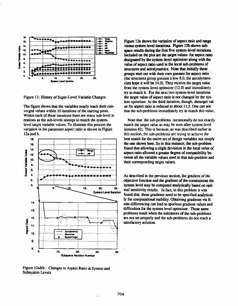
sdulicm strategy 1

701

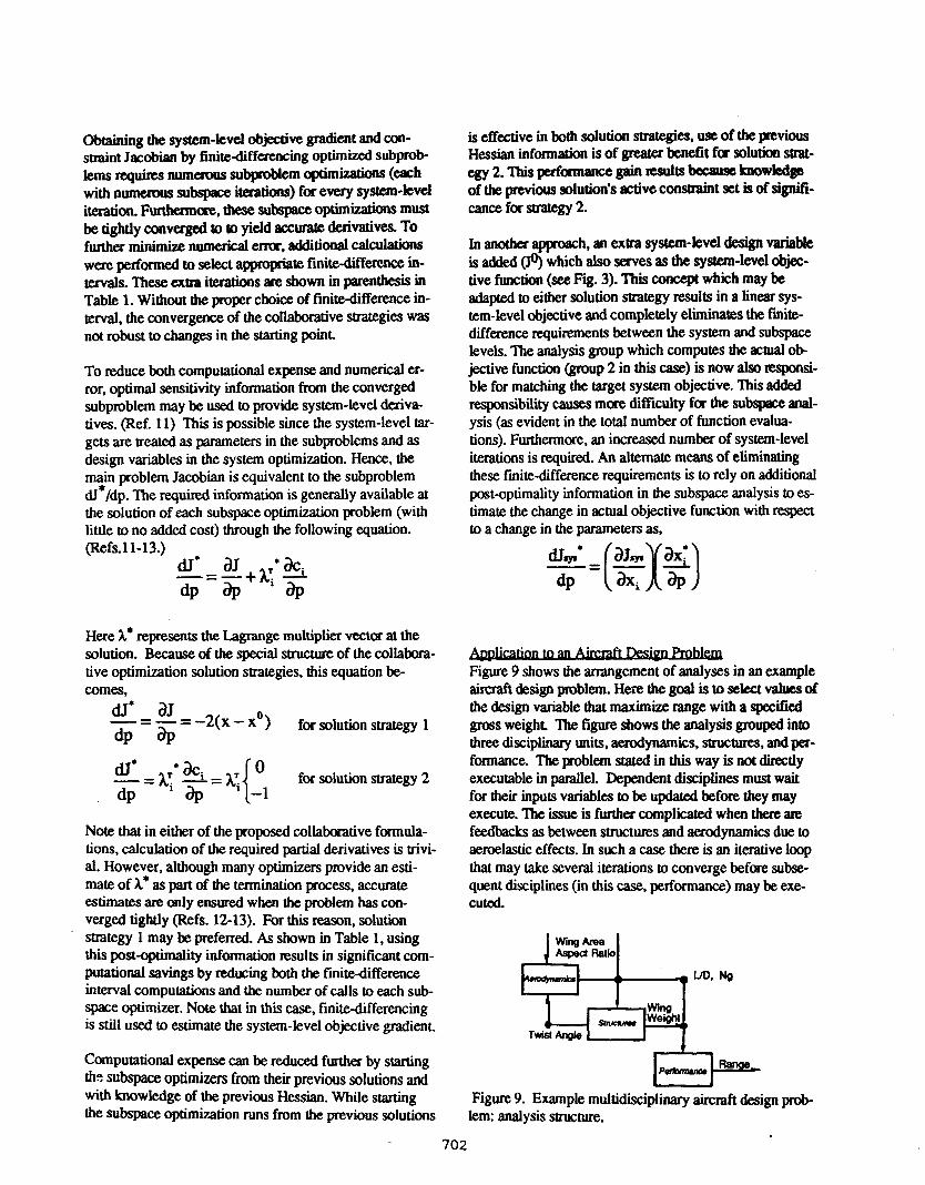
Obtaining the system-kvel objective gradient and constraint Jacobian by finitedifferencing optimized subproblems requires numemu subproblem optimizations (each with numerous subspace iterations) forevery system-kvcl iteration. Fur&hexmcce, these subspace optimizations must be tightly converged to to yield accurate derivatives. To furthet minimize numerical m, additional calculations were performed to s e k t appropriate finitedifference in- tervals. Thw extra iterations are shown in patenthesis in Table 1. Without the proper choice of finitedifference interval, the convergence of the collaborative strategies was not robust to changes in the starting point.

To reduce both computational expense and numerical er- ror, optimal sensitivity information from the converged subproblem may be used to provide system-level derivatives. (Ref. 11) This is possible since the system-level tar- gets are trated as parameters in the subproblems and as design variables in the system optimization. Hence, the ":in problem Jacobian is equivalent to the subproblem dJ /dp. The required information is generally available at the solution of each subspace optimization problem (with little to no added cost) through the following equation. (Refs. 1 1 - 13.)

-=- dP aP

Here A* represents the Lagrange multiplier vector at the solution. Because of the special structure of the collabom- tive optimization solution strategies, this equation becomes,

dJ' aJ 0 - = -= -2(x- x ) dP aP for solution strategy 1

for solution strategy 2 ---+ dJ' -=q aci dP aP

Note that in either of the proposed collaborative formulations, calculation of the required partial derivatives is trivi- al. However, although many optimizers provide an estimate of X* as part of the mination process, accurate estimates are only ensured when the problem has converged tightly (Refs. 12-13). For this reason, solution strategy 1 may be preferred. As shown in Table 1, using this post-optimality information results in significant computational savings by reducing both the finitedifference interval computations and the number of calls to each subspace optimizer. Note that in this case, finitedifferencing is still used to estimate the system-level objective gradient.

is effective in both solution strategies, usc of the pvim Hessian information is of greatex benefit for Soluticm strat-

of the pviow solution's active constraint set is of signifi- egy2. This perfarancegain Fesults~knowwgc

cance for strategy 2.

In another appoach, an extra system-level design variable is added (lo) which also serves as the system-level objective function (see Fig. 3). This concept which may be adapted to either solution strategy results in a linear system-level objective and completely eliminates the fmite- difference requirements between the system and subspace levels. The analysis group which computes the actual ob jective function @roup 2 in this case) is now also responsible for matching the target system objective. n i s added responsibility causes mOre difficulty far the subspace analysis (as evident in the total number of function evalua- tions). Furthermore. an increased number of system-level iterations is required. An alternate means of eliminating these finitedifference requirements is to rely on additional post-optimality information in the subspace analysis to estimate the change in actual objective function with respect to a change in the parameters as,

Figure 9 shows the arrangement of analyses in an example aircraft design problem. Here the goal is to select values af the design variable that maximize range with a specified gross weight. The figure shows the analysis grouped into three disciplinary units, aerodynamics, structures, and performance. The problem stated in this way is not directly executable in parallel. Dependent disciplines must wait for their inputs variables to be updated before they may execute. The issue is further complicated when there axe feedbacks as between structures and aerodynamics due to aeroelastic effects. In such a case there is an iterative loop that may take several iterations to converge before subsequent disciplines (in this case, performance) may be executed.

Computational expense can be reduced furtha by stamng th= subspace optimizers from their previous solutions and with knowledge of the previous Hessian. While starting the subspace optimization runs from the previous solutions

Figure 9. Example multidisciplinary aircraft design problem: analysis structure.

702

As 0 firot aumplc d celtaboraa ‘veapimization,consider minimization of Rosenbrock’s valley function:

min: J(XlJ2) = 100 ( ~ 2 - xl2P + (1 - x ~ P solution of this two-variable, l m c m s m d *

lem with Variousoptimization techniqpes ispresentbdin Ref. 1. In the present analysis, all q t h h t t b isper- f~withthesequentialquadraticprogrammingslgo- rithm, NPSOL. From a stiirhg point of [O.O, 0.01, usiag analytic gradients, NPSOL reached the the solution in 13 iterations. For demonstration purpose% assume that we are dealing with a mOre complex, multidisciplinary optimization problem than the RosenbrocL valley in which the design components are computed by different groups. Al- though this mputat ional ly-di~butcd problem may be reassembled and solved by a single optimizer, one of the significant advantages of coilabcmtive optimization is that this inegration is not necessary. For example, suppose computation of the Roseribrock objective function is decomposed among two groups as,

mix J = J 1 + J2 where: J1 (XI& = 100 ( ~ 2 - ~ 1 ~ ) ~ and: Jz(x1) = (1 - ~ 1 ) 2

Let one analysis grwp be responsible for compnting J1 andamtherJ2 SinCethecomputationisdiseibuted,~~I- labcmuion is required to ensure that the gmups have a consistent description of the design space. Among numerow strategies which achieve the necessary coordination, two example approaches are illustrated in figure 8. In both cases, the system-level optimizer is used to orchessate the o v e d optimization process through selec: tion of system- level met variables. A system-level target is needed for each miable which is usedby more than one analysis group (e%., y1 which is computed in analysis group 1 and input to analysis group 2). The subspace optimizers have as design variables all inputs required by their analysis group. Note that for analysis group 1, this includes the local -le x~ which is natusedinanalysisgrwp2. Thc goal of each subspace optimizer is to minimize the discrepancy between the local versions of each system-level target variable and the target variable itself. Treaunent of this discrepancy minimization is the source of the differences between the two co-ve strategies. In the fust approach (left si& of figure! 8), a summed square discrep ancy is minimized and the collaborative framework does not introduce any additional umstral ‘nts to the analysis group. Note that this subspace objective function is at least quadratic but is generally more nonlinear. In the approach depicted on the right, a constraint is added for each system-level target needed by the analysis group (Ref. 10). If the system-level target is represented locally as an input, this added constraint is l h , otherwise, the added con- saaint is nonlinear. In this formulation, an extra design variable ( x 3 is required and the objective is linear.

Figure 8. Two collaborative optimization approaches for Rosenbmcks valley function

sdulicm strategy 1

701

Obtaining the system-kvel objective gradient and constraint Jacobian by finitedifferencing optimized subproblems requires numemu subproblem optimizations (each with numerous subspace iterations) forevery system-kvcl iteration. Fur&hexmcce, these subspace optimizations must be tightly converged to to yield accurate derivatives. To furthet minimize numerical m, additional calculations were performed to s e k t appropriate finitedifference in- tervals. Thw extra iterations are shown in patenthesis in Table 1. Without the proper choice of finitedifference interval, the convergence of the collaborative strategies was not robust to changes in the starting point.

To reduce both computational expense and numerical er- ror, optimal sensitivity information from the converged subproblem may be used to provide system-level derivatives. (Ref. 11) This is possible since the system-level tar- gets are trated as parameters in the subproblems and as design variables in the system optimization. Hence, the ":in problem Jacobian is equivalent to the subproblem dJ /dp. The required information is generally available at the solution of each subspace optimization problem (with little to no added cost) through the following equation. (Refs. 1 1 - 13.)

-=- dP aP

Here A* represents the Lagrange multiplier vector at the solution. Because of the special structure of the collabom- tive optimization solution strategies, this equation becomes,

dJ' aJ 0 - = -= -2(x- x ) dP aP for solution strategy 1

for solution strategy 2 ---+ dJ' -=q aci dP aP

Note that in either of the proposed collaborative formulations, calculation of the required partial derivatives is trivi- al. However, although many optimizers provide an estimate of X* as part of the mination process, accurate estimates are only ensured when the problem has converged tightly (Refs. 12-13). For this reason, solution strategy 1 may be preferred. As shown in Table 1, using this post-optimality information results in significant computational savings by reducing both the finitedifference interval computations and the number of calls to each subspace optimizer. Note that in this case, finitedifferencing is still used to estimate the system-level objective gradient.

is effective in both solution strategies, use of the pvious Hessian information is of greatex benefit for Soluticm strat-

of the pvious solution's active constraint set is of signifi- egy2. This perfarancegain Fesults~knowwgc

cance for strategy 2.

In another appoach, an extra system-level design variable is added (lo) which also serves as the system-level objective function (see Fig. 3). This concept which may be adapted to either solution strategy results in a linear system-level objective and completely eliminates the fmite- difference requirements between the system and subspace levels. The analysis group which computes the actual ob jective function @up 2 in this case) is now also responsible for matching the target system objective. n i s added responsibility causes mOre difficulty far the subspace analysis (as evident in the total number of function evalua- tions). Furthermore. an increased number of system-level iterations is required. An alternate means of eliminating these finitedifference requirements is to rely on additional post-optimality information in the subspace analysis to estimate the change in actual objective function with respect to a change in the parameters as,

Figure 9 shows the arrangement of analyses in an example aircraft design problem. Here the goal is to select values af the design variable that maximize range with a specified gross weight. The figure shows the analysis grouped into three disciplinary units, aerodynamics, structures, and performance. The problem stated in this way is not directly executable in parallel. Dependent disciplines must wait for their inputs variables to be updated before they may execute. The issue is further complicated when there axe feedbacks as between structures and aerodynamics due to aeroelastic effects. In such a case there is an iterative loop that may take several iterations to converge before subsequent disciplines (in this case, performance) may be executed.

Computational expense can be reduced furtha by stamng th= subspace optimizers from their previous solutions and with knowledge of the previous Hessian. While starting the subspace optimization runs from the previous solutions

Figure 9. Example multidisciplinary aircraft design problem: analysis structure.

702

Posed as a collaborative optimization problem, the design task is decomposedas shown in figure 10. Each ofthedis- ciplinary units becomes an iadependent subproblem. Ehch sub-jmblem cmsisrs of two parts: a subspace optimiza andananalysisroutine. Theoptimizermodifies the input values for the sub-problem analysis and uses the analysis output values to fonn the constraints and objective. The optimizer also accepts a set of target values for these variables. The goal of the subspatx optimization is to adjust the local design variables to minimize the difference between local variable values (both inputs to, and results from, the sub-problem analysis) and the target values passed to the subspace optimizer. To designate these target values the CO methodology adds a system-level optimizer. This optimizer specifies the target values of the design parameters and passes them to each of the subproblems. The system-level optimizer's goal is to adjust the parameter values so that the objective function (in this case, range) is maximized while the system-level constraints are satisfied.

In this problem there are three system-level constraints. Note from the figure that these constraints are simply the values of the objective function of each of the subproblems. Thus, the scheme allows the subproblems to temporarily disagree with each other but the equality constraints (Ji=J2=J3=O) at the system-level qu i r e that in the end, they all agree. So at the end of the optimization all local variable values will be the same as the target values (those with the "0" subscript) designated by the system-level (i.e. Q = R).

xo - & *. A h . phb M o ns.nn*o

For example, assume that the system-level optimizer chooses M initial set of design parameters, %. Each of the sub-lev& will then attempt m match this set Howev- et, if rhe super-level asks for a physically impossible com- bination, then the sub-pmblem will only be able toreturn a m-m value of its objective function J1. This non-zero value is then recognized by the sysem-level and a more feasible choice of target panuneters (X,,) is selected. This next set allows the sub-problem to obtain a minimum objective function (J 1) lower than with the previous set. It is through such a mechanism that the sub-pblems influence the progress of the design optimization.

Via a similar mechanism, constraints that exist at the sub-pblem level may influence the target (system-level) variable values, and, through this, the value used in another discipline. In this way, constraints that affect one discipline may implicitly affect another without the need for an explicit transfer of information concerning the constraint to a foreign discipline.

One of the primary advantages of this arrangement is that the system is now executable in parallel. In fact, this architecture minimizes the interdiscipinary communication requirements, making it ideal for network implementa- tions. This example problem has been run both on a single workstation and on a system of three ne€wded com- puters.

Results Figure 11 shows the optimization history of the design

variables. Range was computed by the performance analysis using the B r e w range equation. Wing weight was computed using statistically-based equations for typical weights of transport aimraft wings given maximum load factor, aircraft weights, and wing geometry. The twist an- gle was also calculated by the structures discipline. It rep resents the maximum structural twist of a wing under cer- tain aerodynamic loads. These twists are computed for a given maximum gust loading which is calculated in the aerodynamics discipline. The twist itself feeds back into the aerodynamics discipline and changes aerodynamic loading on the wing. The aerodynamics discipline uses simple relations to produce the aerodynamic loading and the lift-todrag ratio (used in calculating range).

Figure 10. Collaborative form of aircraft design problem.

703

f le. ia 14.

12

1 0.

2 0.

i .....

0. 5. 10. 15. 2Q. sv*wnLmlnudion

Figure 11: History of Sup-Level Variable Changes

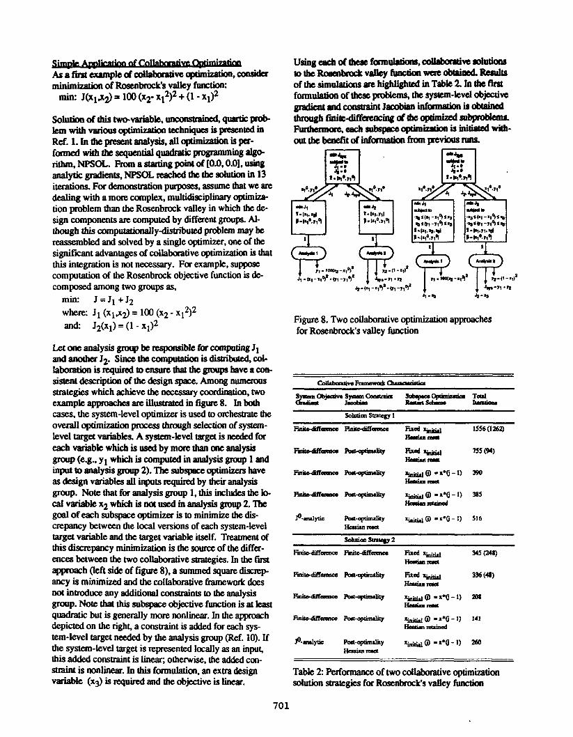
The figure shows that the variables nearly reach theit converged values within 10 iterations of the starting point Within each of these iterations there are many sublevel iterations as the sublevels attempt to match the system- level target variable values. To illustrate this prccess the variation in the parameter aspect ratio is shown in Figure 12a and b.

18.

16.

14.

B: 2.

0.

14.

I ............ .................... ........... .. ............ ............................... .................... 1 1

4 5.-

.......................... .......................... ..... .................. + .......................... i i

12.

E ::: 9.

. . . . . . , : i , . . I . . ....... ... i.. ...,.. . ,.-... L.; - .......................... ....... :. - ;'

- . : I - . - -. :

...... c .................. .......................... .......................... ................. i ..... :.r.--

:' Y .................... .......................... ...... ; ............. .......

.......................... ..... 1 I ......-..-..........+..........................+.......................... I 1 . 8. ' I

0. 10. 20. 30. 40. subspace Heration Number

Figure 12a shows the variation of aspect mtio and range

space nsults during the first five system-level iterations. s~&em-level itarations. Fig~r! 12b shows sub

Included on the plot an the targu values for aspect ratio

value of aspect ratio used in the bcal sub-@lms of designated by t h ~ ~ystem-levcl OpimiZer along With the

structures and acmdynamics. Note that mitially these groups start out with their own guesses for aspect ratio (the structures group guesses a low 8.0, the aerodynami- cists hope it will be 14.0). They receive the target value from the system-level optimizer (12.0) and immediately try to match it. For the next two system-level iterations the targa value of aspect ratio is not changed by the system optimizer. At the third iteration, though, themget value for aspect ratio is red& to about 11.5. One can see that the sub-problems immediately try to match this value.

Note that the subproblems occasionally do not exactly match the target value as may be seen after system-level iteration #2;. This is because, as was described earlier in this section, the subproblems are trying to achieve the best match far the entire set of design variables not simply the one shown here. So in this instance, the sub-problem found that allowing a slight deviation in the local value of aspect ratio allowed a greates degree of Compatibility between all the variable values used in that sub-problem and their corresponding target values.

As describexi in the previous section, the gradient of the objective function and the gradient of the COllstraJn *tsatthe system level may be computed analytically based on optimal sensitivity results. In fact, in this problem it was found that these gmdients need to be specified analytically for computational stability. Obtaining gradients via finitedifferencing can lead to spurious gradient values and difficulties for the system level optimizer. These same problems result when the tolerances of the sub-problems are not set properly and the sub-problems do not reach a satisfactory solution.

Figure 12a&b : Changes in Aspect Ratio at System and Subsystem Levels

704

whether the analysis is decomposed using compatibility constraints, artbe design poMem is dccoarposed using collaborativeopimization,thesaucturedthedccomposi- tiondetenninestheefficiencyofthedecomposedsyslem For example, consider two subroutines with wmputath timesA andB,withn hputstoA,andm intermediate values computed by A which m inputs to B. To compute gradients of quantities computed by B with respect to the inputs of A , the computational time using finite differences is n(A+B). If we use decomposition. the computation time for all the gradients becomes nA + mB. When n is much larger than m (contraction), decomposition will generally reduce computation time. If, however, m is larger than n, decomposition may increase computation time. Such ideas were considered in the decomposition of the aircraft design problem in figure 4, but only in a qualita- tive fashion. Moreover. the ad hoc procedure was quite time-consuming. To exploit contraction, avoid expansion, and assign analyses to subproblems efficiently, an automatic tool is desirable. Such a program is described here. It uses a genetic algorithm to find a decomposition that minimizes the estimated computational time of a gradient- based optimization of the resulting decomposed system.

Given a list of analyses and the global variables which are inputs and outputs to each, the program creates ahpea- dence matrix of integers. The element Dep(ij) corre sponds to the number of outputs fnnn routine i which are inputs to routine j . If the routines are executed sequential- ly, entries in Dep which are below the main diagonal are feedbacks, and entries above the main diagonal im feed- forwards. As theordersoftheroutinesarechanged, the structures of the dependence matrix changes. By includ- ing infomation about where in the ordering there are "breaks" between subpmblems, various objective functions can be evaluated from the dependence matrix.

Several methods for task-ordering have been developed previously, but not with the objective of scheduling the optimization of a decomposed system. The Design Man- ager's Aid, DeIvfaid (Ref. 2). for example, uses a heuristic approach to order tasks into a system of subproblems. One of the results of the DeMaid heuristic is that feedback loops, particularly long loops, are removed. Figure 13 il- lustrates the ordering of tasks, as described in reference 2, that minimizes a m u r e of feedback extent, J. The objective function used here is:

n i -1 -- J = A 2 Dep (i j) (i-j)

i = l j = l

and reflects the "total length of feedback" in the system. The solution shown in Figure 13, was obtained by the

present SChtQling algorithm using this objc€tivc. It is nearly identical to theoneobtakdby DeMaid, which does not employ an explicit objective function. Although the subppobkmsare in adiffereat ordet, cach Consists of

second,which is aunionof twosubproblems from t h e b Maid solutioh

I " I I I I I

thcsamcanal~as m the DeMaidpoblem,exceptthe

Figure 13. Solution of the DeMaid example problem us- mg extent of feedback as objective function.

Minimizing feedback exm is not the goal for a system

timization. The difference between feedback and feedfor-

Therefore the length of an individual feedback is unimpor- tant, and some feedback benveen the subproblems is not disadvantageous. Conversely, the number of feedforwads between subproblems is important. Thus, a rather different objective is used for the optimal decomposition formulation. The objective used here is an explicit estimate of the computation time for optimization of the decomposed designproblem.

that is decomposed using compatibility constraints and op-

ward disappeafs, since the subproblems run in parallel.

The time estimate assumes the following about the optimization of the system: gradients are estimated by finitedifferencing, no secondderivatives are computed (the estimated Hessian is updated); and gradient calculations dominate the computation time. These assumptions are consistent with aircraft sizing problems and with the use of NPSOL, a commonly used optimization package. In addition, it is assumed that the subproblems can be executed in parallel. Finally,we assume that gradients for a subproblem depend on all routines within that subproblem.

The objective function is then: = Toptimiation = @he searches) * peach line search)

N h e -,.hes is proportional to the total number of vari-

705

abies. Therdore the numbex of line searches varies as: %ne searches =%esign vars + Nauxiliary design vars

For a typical gradient-based optimization each line search requires that each subroutine be executed once for cach independent variable (for gradients) and then an averaw of twice more for the line search itself. Ihe taal numbex of calls tothemtinesineachgroup is the= N* = * + Ndesign vars(sub i) + Nauxiliary var (sub i)

where N~Q.,, vars (sub i) is the number of design variables that are inputs to routines in the i h subpr~blem. Since the subproblems are run in parallel, the time for each line search is determined by the slowest subproblem: T b e i = max (Ncalls, * X(execution times of routines in subproblem i))

12

BIUL

Subroutine 9

Subroutine 6 Subroutine 4

BlUk

Subroutine 5 Subroutine 8

Genetic Independent String Subtasks

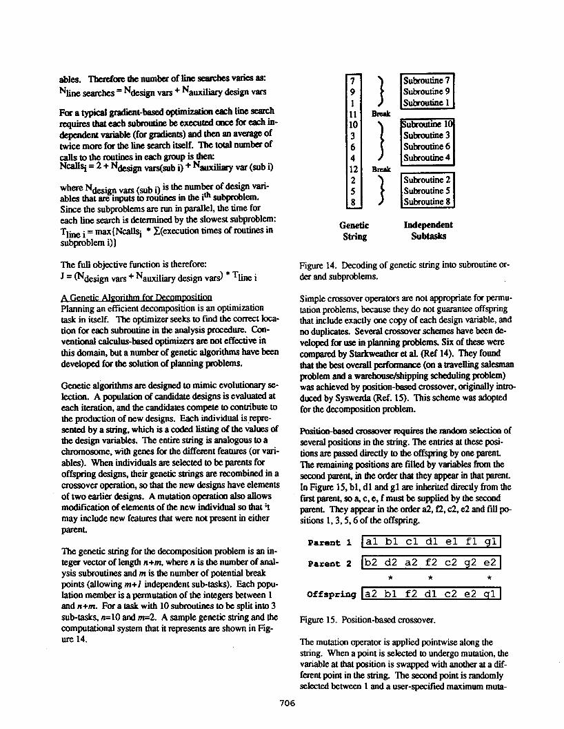
The full objective function is therefore: Figure 14. Decoding of genetic string into subroutine order and subproblems. = mdesign v a n + Nauxiliary design vars) * i

Planning an efficient decomposition is an optimization task in itself. The optimizer seeks to find the correct loca- tion for each subroutine in the analysis procedure. Con- ventional calculus-based optimizers are not effective in this domain, but a number of genetic algorithms have been developed for the solution of planning problems.

Genetic algorithms are designed to mimic evolutionary selection. A population of candidate designs is evaluated at each iteration, and the candidates compete to contribute to the production of new designs. Each individual is represented by a String. which is a coded listing of the values of the design variables. The entire string is analogous to a chromosome. with genes for the different features (or variables). When individuals am selected to be parents for offspring designs, their genetic strings are recombined in a crossover operation, so that the new designs have elements of two earlier designs. A mutation operatian also allows modification of elements of the new individual so that ;t may include new features that were not present in either parent.

The genetic smng for the decomposition problem is an in- teger vector of length n+m. where n is the number of analysis subroutines and m is the number of potential break points (allowing m+l independent subtasks). Each population member is a permutation of the integers between 1 and n+m. For a task with 10 subroutines to be split into 3 sub-tasks, n=10 and -2. A sample genetic string and the computational system that it represents are shown in Fig- ure 14.

Simple crossover operators are not appropriate for permutation problems, because they do not guarantee offspring that include exactly one copy of each design variable, and no duplicates. Several crossover schemes have been developed for use in planning problems. Six of these were compared by Starkweather et al. (Ref 14). They found that the best overall performance (on a travelling salesman problem and a warehouse./shipping scheduling problem) was achieved by position-based crossover, originally introduced by Syswexda (Ref. 15). This scheme was adopted for the decomposition problem.

position-based cmssovef requires the randoin selection of several positions in the string. The entries at these positions are passed directly to the offspring by one parent. The remaining positions are filled by variables from the second parent, in the order that they appear in that parent. In Figure 15, bl, dl and gl are inherited directly from the firs parent, so a, c,e, f must be supplied by the second parent. They appear in the order a2, f2, c2, e2 and fill positions l, 3,5,6 of the offspring.

Parent 1 t a l b l e l d l e l f l gll

Parent 2 lb2 d2 a2 f2 c2 92 e21 * * *

Offspring [a2 b l f 2 d l c 2 e2 gl1

Figure 15. Position-based crossover.

'Ihe mutation operator is applied pointwise along the string. When a point is selected to undergo mutation, the variable at that position is swapped with another at a different point in the string. ' he second point is randomly selected between 1 and a user-specified maximum muta-

706

tion range. Thc gcndic algorithm use8 twrnament Seh- tion to choose p n o to participate in repductirn into the next generation. Each time a patent is needed, two membea of the carrent population am selected at random. Their fitness is competed, and the individual with greata f i ~ b e ! c ~ t h e ~ t .

'Ihe following parametex settings were used in studies re-

wise mutation probability is 0.01: and maximum muration range is half the total string length, or (n+m)/2.

ported here: CTOSSOVW probslbility i~ fixed Bt o.% p ~ h t -

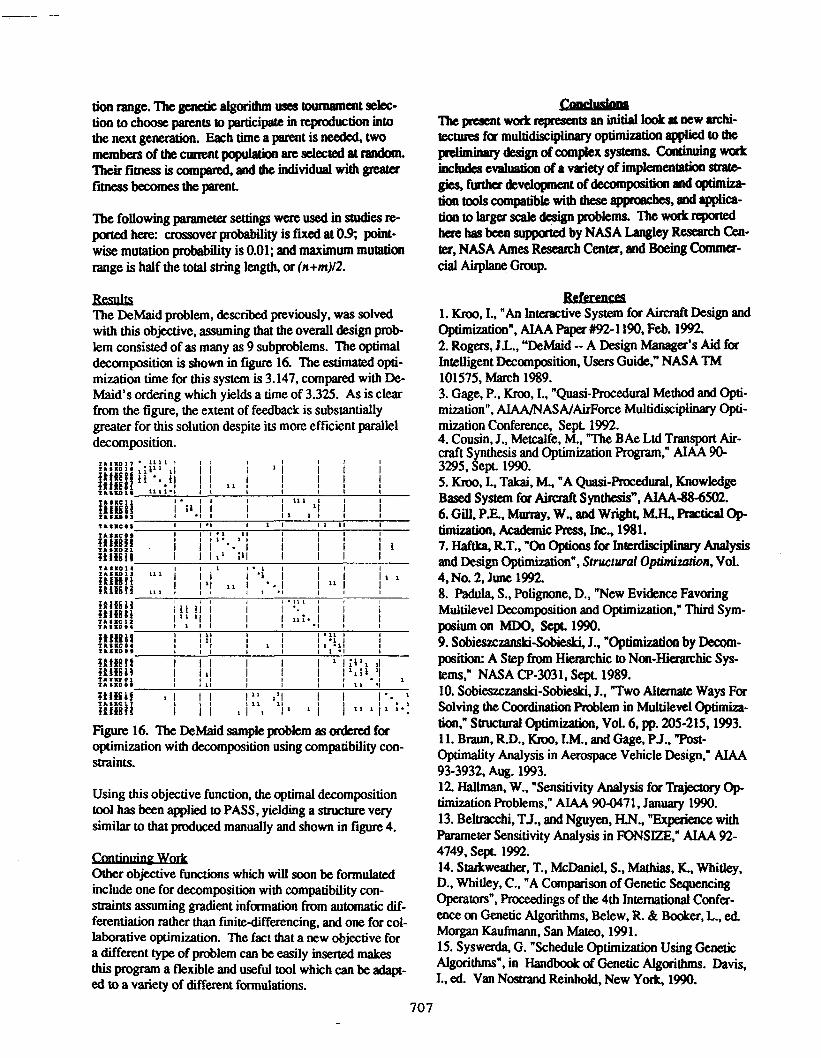
Results The DeMaid problem, described previously, was solved with this objective, assuming that the overall design problem consisted of as many as 9 subproblems. The Optimal decomposition is shown in figure 16. The estimated optimization time for this system is 3.147, compared with De- Maid's ordering which yields a time of 3.325. As is clear from the figure, the extent of feedback is substantially greater for this solution despite its more efficient parallel decomposition.

figure 16. 'Ihe DeMaid sample problem as ordered for optimization with decomposition using compatibility constraints.

Using this objective function, the optimal decomposition tool has been applied to PASS, yielding a structure very similar to that produced manually and shown in figure 4.

Other objective functions which will soon be formulated include one for decomposition with compatibility constraints assuming gradient information from automatic dif- ferentiation rather than fmite-differencing, and one for collaborative optimization. The fact that a new objective for a different type of problem can be easily inserted makes this program a flexible and useful tool which can be adapted to a variety of different formulations.

cmdJukm

peliminerydesignofcomplexsystems. ContirmingWorL

gits,fiathadevtlapnentof~positionandapimiza-

tion to hgex scale dcsign probkms. m work reported

'Ihe present work repnsenar an initial look at new archi- ttctures far multidisciplinary optimization applied to the

includes evaluation of a variety of implementation strate

th tools compatible with dKse appoaches, and appiiCa-

here has betn supparted by NASA Langley Research Cen-

cial Airplane Group. ter, NASA A m e ~ R-h Cater, and Boeing COmmer-

Relerenees 1. h, 1.. "An Interxtive System for Aimaft Design and Optimization", AIAA Paper #92-1190, Feb. 1992. 2. Rogers, JL., "&Maid -- A Design Manager's Aid for Intelligent Decomposition, Users Guide," NASA TM 101575, March 1989. 3. Gage, P., Kroo, I., "Quasi-F'rocedural Method and Opti- mization", AIAAJNASA/AirForce Multidisciplinary Oph- mization Conference, Sept 1992. 4. Cousin, J., Metcalfe, M., "The BAe Ltd Transport Air- craft S thesis and Optimization Rogram," AIAA 90-

Based System for Airaaft Synthesis", AIAA-88-6502. 6. Gill. PL, Murray, W., and Wright, M.H., practical Op hmnatmn, Academic Press, Inc., 1981. 7. Haftka, RT., "On Options for Interdisciplinaty Analysis and Design Optimization", Srructural Optimitnrion, Vol. 4, No. 2, June 1992. 8. Padula, S., Polignone, D., "New Evidence Favoring Multilevel Decomposition and Optimization," Third Sym- posium on MDO, Sep. 1990. 9. Sobieszczanski-S, J., "Optimization by Decgm- position: A Step from Hienuchic to Non-Hierarchic Sys-

10. Sobieszczanslu '-Sobieski, J., "Two Alternate Ways For

3295, !g.& 1990. 5. h, I., Takai, M., "A Quasi-procedural, Knowled@

. . .

tem~." NASA CP-3031, S q t . 1989.

Solving the Coordination problem in Multilevel O p t i d - tion," StrUchn;il opbmization, Vol. 6, p ~ . 205-215,1993. 11. Braun, R.D., KIUO, I.M.. and Gage, PJ., "Post- Optimality Analysis in Aerospace Vehicle Design," AIAA

12 Hallman, W., "Sensitivity Analysis for Trajectoxy Op timization Problems," AIAA 90047 1, January 1990. 13. Beltracchi, TJ., and Nguyen, HN., "Experience with F'arameter Sensitivity Analysis in FONSIZE," AIAA 92- 4749, Sep. 1992. 14. Starkweather. T., McDaniel, S., Mathias, K, Whitley. D., Whitley, C., "A Comparison of Genetic Sequencing Operators", proceedings of the 4th International Confer- ence on Genetic Algorithms, Belew, R. & Booker, L., ed Morgan Kaufmann, San Mateo, 1991. 15. Syswetda. G. "Schedule Optimization Using Genetic Algorithms", in Handbook of Genetic Algorithms. Davis, I., ed. Van Nosaand Reinhold, New Yorlr, 1990.

93-3932, AUg. 1993.

70 7

MUI,IDBCIPLINARY OPTIMIZATION METHODS FOR AIRCRAFT PRhWMINARY … · MUI,"IDBCIPLINARY OPTIMIZATION METHODS FOR AIRCRAFT PRhWMINARY DESIGN by Ilan Kroo, Steve Altus, Robert Braun,

Documents