arXiv:physics/0603035v1 [physics.bio-ph] 6 Mar 2006 SIMULATIONS IN STATISTICAL PHYSICS AND BIOLOGY: SOME APPLICATIONS María del Pilar Monsiváis-Alonso M.Sc. Thesis Supervisors: Dr. Román López-Sandoval Dr. Haret-Codratian Rosu Division of Advanced Materials for Modern Technology DMATM -IPICyT San Luis Potosí, S.L.P., Mexico January 20, 2006

Welcome message from author
This document is posted to help you gain knowledge. Please leave a comment to let me know what you think about it! Share it to your friends and learn new things together.
Transcript
arX
iv:p
hysi
cs/0
6030
35v1
[ph
ysic
s.bi
o-ph
] 6
Mar
200
6
SIMULATIONS IN STATISTICAL PHYSICS
AND BIOLOGY: SOME APPLICATIONS
María del Pilar Monsiváis-Alonso
M.Sc. Thesis
Supervisors:
Dr. Román López-Sandoval
Dr. Haret-Codratian Rosu
Division of Advanced Materials
for Modern Technology
DMATM -IPICyT
San Luis Potosí, S.L.P., MexicoJanuary 20, 2006
INSTITUTO POTOSINO DE INVESTIGACIÓN
CIENTÍFICA Y TECNOLÓGICA, A.C.
POSGRADO EN CIENCIAS APLICADAS
SIMULATIONS IN STATISTICAL PHYSICS
AND BIOLOGY: SOME APPLICATIONS
Tesis que presenta
María del Pilar Monsiváis-Alonso
Para obtener el grado de
Maestro en Ciencias Aplicadas
En la opción de
Nanociencias y Nanotecnología
Codirectores de la Tesis:
Dr. Román López-Sandoval
Dr. Haret-Codratian Rosu Barbus
San Luis Potosí, S.L.P., 20 de Enero de 2006

Acknowledgments
First of all, I would like to thank my advisor Dr. Román López Sandoval for his dedication, guidance andconstant support during the development of this thesis. In the same spirit, I would like to thank my advisor Dr.Haret Codratian Rosu Barbus for his suggestions.
I also want to acknowledge the PhD student Vrani Ibarra for his important collaboration referring to chapter 3of this thesis and I am also grateful to Dr. José Luis Rodríguez, Dra. Yadira Vega and Dr. Raúl Balderas, whoread the document and provided helpful corrections.
I would like to thank in a special way to my parents, who alwayshave been a support for me in everything,as well as, to Jorge and all my friends, in particular José Miguel, Víctor Hugo, Andrea, Gerardo, Pedro andVianney.
My final thanks go to CONACyT for the master fellowship (no. 182493) during the years 2003-2005.
THANKS ALL OF YOU!
Pily Monsiváis
iii

Contents
Acknowledgments iii
Abstract vi
Introduction 1
Introduction 1
1 Monte Carlo Simulations in Statistical Physics 31.1 Brief History of the Monte Carlo Method . . . . . . . . . . . . . . .. . . . . . . . . . . . . 41.2 Basics of the Monte Carlo Method . . . . . . . . . . . . . . . . . . . . .. . . . . . . . . . . 61.3 Measurements Using the Monte Carlo Method . . . . . . . . . . . .. . . . . . . . . . . . . . 81.4 Ising and Potts Models . . . . . . . . . . . . . . . . . . . . . . . . . . . . .. . . . . . . . . 91.5 Some Monte Carlo Algorithms: Metropolis, Swendsen-Wang and Wolff . . . . . . . . . . . . 101.6 Phase Transitions and Critical Exponents . . . . . . . . . . . .. . . . . . . . . . . . . . . . 131.7 The Histogram Method . . . . . . . . . . . . . . . . . . . . . . . . . . . . . .. . . . . . . . 161.8 Identifying the Nature of Transitions and Finite Size Scaling . . . . . . . . . . . . . . . . . . 181.9 Monte Carlo Simulations on the Betts Lattice . . . . . . . . . .. . . . . . . . . . . . . . . . 21
1.9.1 q= 3, J < 0: Antiferromagnetic Case . . . . . . . . . . . . . . . . . . . . . . . . . . 221.9.2 q= 3, J > 0: Ferromagnetic Case . . . . . . . . . . . . . . . . . . . . . . . . . . . . 251.9.3 q= 4, J > 0: Ferromagnetic Case . . . . . . . . . . . . . . . . . . . . . . . . . . . . 291.9.4 q= 5, J > 0: Ferromagnetic Case . . . . . . . . . . . . . . . . . . . . . . . . . . . . 321.9.5 Conclusion . . . . . . . . . . . . . . . . . . . . . . . . . . . . . . . . . . . .. . . . 35
2 Monte Carlo Simulations in Biology 362.1 Proteins, DNA and Gene Expression . . . . . . . . . . . . . . . . . . .. . . . . . . . . . . . 372.2 DNA Microarrays . . . . . . . . . . . . . . . . . . . . . . . . . . . . . . . . . .. . . . . . . 382.3 Gene Clustering . . . . . . . . . . . . . . . . . . . . . . . . . . . . . . . . . .. . . . . . . . 39
2.3.1 Hierarchical Clustering . . . . . . . . . . . . . . . . . . . . . . . .. . . . . . . . . . 412.3.2 K-Means Clustering . . . . . . . . . . . . . . . . . . . . . . . . . . . . .. . . . . . 422.3.3 Self-Organizing Maps . . . . . . . . . . . . . . . . . . . . . . . . . . .. . . . . . . 422.3.4 Self-Organizing Tree Algorithm . . . . . . . . . . . . . . . . . .. . . . . . . . . . . 422.3.5 Model Based Clustering . . . . . . . . . . . . . . . . . . . . . . . . . .. . . . . . . 432.3.6 Quality-Based Algorithms . . . . . . . . . . . . . . . . . . . . . . .. . . . . . . . . 442.3.7 Adaptive Quality-Based Clustering . . . . . . . . . . . . . . .. . . . . . . . . . . . 452.3.8 Biclustering and Some Physics Related Algorithms . . .. . . . . . . . . . . . . . . . 45
2.4 Superparamagnetic Gene Clustering: Monte Carlo Simulations . . . . . . . . . . . . . . . . . 462.4.1 Detailed Description of SPC . . . . . . . . . . . . . . . . . . . . . .. . . . . . . . . 472.4.2 Future Directions . . . . . . . . . . . . . . . . . . . . . . . . . . . . . .. . . . . . . 48
iv

3 Gompertz Equation 493.1 History of Gompertz Equation . . . . . . . . . . . . . . . . . . . . . . .. . . . . . . . . . . 503.2 Tumour Growth Equations . . . . . . . . . . . . . . . . . . . . . . . . . . .. . . . . . . . . 54
3.2.1 Exponential Growth . . . . . . . . . . . . . . . . . . . . . . . . . . . . .. . . . . . 553.2.2 Logistic Growth . . . . . . . . . . . . . . . . . . . . . . . . . . . . . . . .. . . . . 573.2.3 Von Bertalanffy Growth . . . . . . . . . . . . . . . . . . . . . . . . . .. . . . . . . 593.2.4 Gompertz-Makeham Growth . . . . . . . . . . . . . . . . . . . . . . . .. . . . . . . 603.2.5 Mathematical Properties and Comparison Between Logistic and Gompertz Growth . . 61
Appendix A: Control Theory Fundamentals 63
Bibliography of Chapter 1 65
Bibliography of Chapter 2 71
Bibliography of Chapter 3 75

Abstract
One of the most active areas of physics in the last decades hasbeen that of critical phenomena, and Monte Carlosimulations have played an important role as a guide for the validation and prediction of system properties closeto the critical points. The kind of phase transitions occurring for the Betts lattice (lattice constructed removing1/7 of the sites from the triangular lattice) have been studiedbefore with the Potts model for the valuesq= 3, ferromagnetic and antiferromagnetic regime. Here, we add up to this research line the ferromagneticcase forq = 4 and 5. In the first case, the critical exponents are estimated for the second order transition,whereas for the latter case the histogram method is applied for the occurring first order transition. Additionally,Domany’s Monte Carlo based clustering technique mainly used to group genes similar in their expression levelsis reviewed. Finally, a control theory tool –an adaptive observer– is applied to estimate the exponent parameterinvolved in the well-known Gompertz curve. By treating all these subjects our aim is to stress the importanceof cooperation between distinct disciplines in addressingthe complex problems arising in biology.
vi

Introduction
“Minerals grow, plants grow and live,animals grow, live and have feeling.”Linnaeus, “Systema Naturae”, 1735
Monte Carlo simulations have been used for many years to study the properties of physical models, and havealso played a significant role in statistics, biology, computer science and other fields, demonstrating its versalityand powerful approach. Furthermore, many advances in computation algorithms and computer technologyhave made possible to study systems which would be impossible to examine only a few years ago. Thefirst part of this thesis aims to give a brief explanation of the Monte Carlo method, a review of the principalalgorithms used, the study of phase transitions, finite sizescaling theory and finally, some results obtained withthe Potts model for a recently proposed lattice named Betts or Maple Leaf lattice.
Since the discovery of the helical structure of DNA and various complete genome sequences, biology has seenalso an enormous advance. However, it seems that the only wayto solve the complex problems raised in thestudy of biological systems is to share the challenge with other scientific disciplines such as chemistry, physics,and computer science. Research on cancer is one of the most important and interesting subjects in Biology.This terrible disease has received tremendous attention inthe last part of the XX century, because of the hugeamount of cases and the technological advances in analysis and medical treatment of tumours. Despite theefforts of the international scientific community, there are many unanswered questions related to the evolutionof the cancer diseases, the causes that trigger them, the prediction of drugs and treatments effects, and thedevelopment of an effective cure. The introduction of the Monte Carlo method into biological problems hasbrought interesting results including the modeling of the structure and evolution of a epidermis cell nuclei,reproducing cancer growth.
The second chapter reviews the clustering techniques commonly used to group genes with similar behaviour intheir expressions across various experiments, which helpsin the construction of genetic networks and targetingof genes involved in diseases like cancer. The superparamagnetic gene clustering algorithm is also explainedas an example of a clustering technique that employs the Monte Carlo method and is based on a physicalphenomenom, leaving the subject to future implementation.
On the other hand, mathematical procedures, in particular models based on differential equations whose termscan represent not only the growth rate of a tumour, but also the growth or inhibition rates of substances existingin the medium or cell-cell interactions, provide an excellent tool to describe biological processes. There alsoexist empirical models that have proved to be very useful in fitting the experimental growth curves of tumours.The Gompertz model is a famous one, although there is not a convincing explanation of why it works so well.The Gompertz growth law has been introduced by Benjamin Gompertz in 1825 in his demographical studies,and in mathematical terms is written:
λ (a) = h0eγa, (1)
whereλ (a) is the mortality rate.
The main problem is that the biological interpretation of its characteristic parameters is not very well settled.A link of these parameters with the biological phenomenology, if found, would make the Gompertz model
1

extremely valuable as a predictive tool. The third part of this thesis discusses some of the most importantmodels based on differential equations and gives a more complete idea about the formulation and applicationsof the Gompertz model, and finally presents a method based on control theory capable of accurately predictthe first stages of Gompertz growth.
The main purpose of this work is to emphasize the importance of an interdisciplinary research. Nowadays, it isclear that many problems inherent to the biology field need tobe adressed with tools coming from areas suchas computational physics and applied mathematics.

Chapter 1
Monte Carlo Simulations in StatisticalPhysics
Contents
1.1 Brief History of the Monte Carlo Method . . . . . . . . . . . . . . . . . . . . . . . . . . 4
1.2 Basics of the Monte Carlo Method . . . . . . . . . . . . . . . . . . . . .. . . . . . . . . 6
1.3 Measurements Using the Monte Carlo Method . . . . . . . . . . . .. . . . . . . . . . . 8
1.4 Ising and Potts Models . . . . . . . . . . . . . . . . . . . . . . . . . . . . .. . . . . . . 9
1.5 Some Monte Carlo Algorithms: Metropolis, Swendsen-Wang and Wolff . . . . . . . . . 10
1.6 Phase Transitions and Critical Exponents . . . . . . . . . . . .. . . . . . . . . . . . . . 13
1.7 The Histogram Method . . . . . . . . . . . . . . . . . . . . . . . . . . . . . .. . . . . . 16
1.8 Identifying the Nature of Transitions and Finite Size Scaling . . . . . . . . . . . . . . . 18
1.9 Monte Carlo Simulations on the Betts Lattice . . . . . . . . . .. . . . . . . . . . . . . . 21
1.9.1 q= 3, J < 0: Antiferromagnetic Case . . . . . . . . . . . . . . . . . . . . . . . . . 22
1.9.2 q= 3, J > 0: Ferromagnetic Case . . . . . . . . . . . . . . . . . . . . . . . . . . . 25
1.9.3 q= 4, J > 0: Ferromagnetic Case . . . . . . . . . . . . . . . . . . . . . . . . . . . 29
1.9.4 q= 5, J > 0: Ferromagnetic Case . . . . . . . . . . . . . . . . . . . . . . . . . . . 32
1.9.5 Conclusion . . . . . . . . . . . . . . . . . . . . . . . . . . . . . . . . . . . .. . . 35
3

1.1 Brief History of the Monte Carlo Method
The first electronic computer, ENIAC, was developed during the World War II period by a group of scientistsworking at the University of Pennsylvania in Philadelphia.They had realized that if electronic circuits could bemade to count, then they could do arithmetic and hence, solvedifference equations at incredible speeds. Thiswould lead to a scientific revolution because it would give the possibility to study problems unsolved beforedue to the large amount of calculations needed.
In 1946, Stanislaw Ulam, a mathematician working in Los Alamos, attended a conference about a preliminarycomputational model of a thermonuclear reaction probed in ENIAC as a test for the computer. Like otherscientists, he was impressed by the speed and versatility ofthe ENIAC. Additionally, Ulam’s extensivemathematical background made him aware that statistical sampling techniques that had fallen into disusebecause of tediousness of calculations, could be resuscitated with ENIAC. The basis of the Monte Carlo methodhas been proposed later by him as a consequence of his interest in random processes. As Stan Ulam mentionedin 1983, his first thoughts and attempts to practice the MonteCarlo method were suggested by a question thatoccurred to him in 1946 as he was playing solitaires. The question was what were the chances that a Canfieldsolitaire laid out with 52 cards will come out succcessfully? 1. After spending a lot of time trying to estimatethem by pure combinatorial calculations, he wondered whether a more practical method might not be to layit out say one hundred times and simply observe and count the number of successful plays. He immediatelythought about how to change processes described by certain differential equations into an equivalent forminterpretable as a succession of random operations [1]. Ulam discussed his ideas with John von Neumann,Professor of Mathematics at the Institute for Advanced Study at Princeton, who was also a consultant to LosAlamos and one of the principals participating in the ENIAC probe conference in 1946. Von Neumann sawthe importance of Ulam’s approach and thought that it seemedespecially suitable for exploring the behaviourof neutron chain reactions in fission devices. In March 1947,von Neumann wrote to Robert Richtmyer, theLeader of the Theoretical Division at Los Alamos, describing a possible statistical method to solve the problemof neutron diffusion in fissionable material using the newlydeveloped electronic computing techniques. It wasat that time when Nicholas Metropolis suggested the name Monte Carlo for this statistical method. It wasrelated to the fact that Stan had an uncle who would borrow money from relatives because he “just had to go toMonte Carlo” [2] and also because of the similarities between the method and the games of chance abundantin the capital of Monaco, the european center of gambling.
Very similar methods, not fully developed, had been used earlier. An example is Buffon’s needle problem, anexperiment performed in the of the eighteenth century, which represents one of the first problems in geometricprobability. It consists in throwing a needle randomly on a board with parallel lines, and inferring the value ofπ from the number of times the needle intersects a line [3]; nowadays, Buffon’s needle problem is practicallysolved by Monte Carlo integration. Descriptions of severalmodern Monte Carlo techniques appear in a paperby Kelvin [4], written nearly one hundred years ago, in the context of a discussion on the Boltzmann equation.In the 1940’s, Enrico Fermi also used Monte Carlo in the calculation of neutron diffusion, and later designedthe Fermiac, a Monte Carlo mechanical device used in the calculation of criticality in nuclear reactors [5].Ulam’s contribution was to recognize the potential for the newly invented electronic computer to automatesuch sampling.
The approach proposed by von Neumann in his letter was the first formulation of a Monte Carlo computationfor an electronic machine. Von Neumann considered a spherical core of fissionable material surrounded bya shell of normal material, and the idea was to trace out the development of neutrons using random digits toselect the outcomes of the various interactions along the way, such as scattering, absorption and fission. Forexample, once a neutron is selected to have an initial position with certain velocity, you have to decide theposition of the first collision and the nature of the collision. If you select a fission to occur, then the numberof emerging neutrons must be chosen, and each of the new neutrons is followed too. On the other hand, if youdecide that the outcome of the collision is scattering, the new momentum of the neutron must be determined.
1Today is quite well known that the chance of winning is low: 3.3% (www.games.solitaire.com)
If the neutron crosses a material boundary, the characteristics of the new medium must be taken into account.At the end, a genealogical history of a neutron emerges. The same procedure is carried out for other neutronsuntil a statistically valid picture is obtained. Each neutron history is analogous to a single game of solitaire,and the use of random numbers to make the choices along the wayis analogous to the random turn of the card.
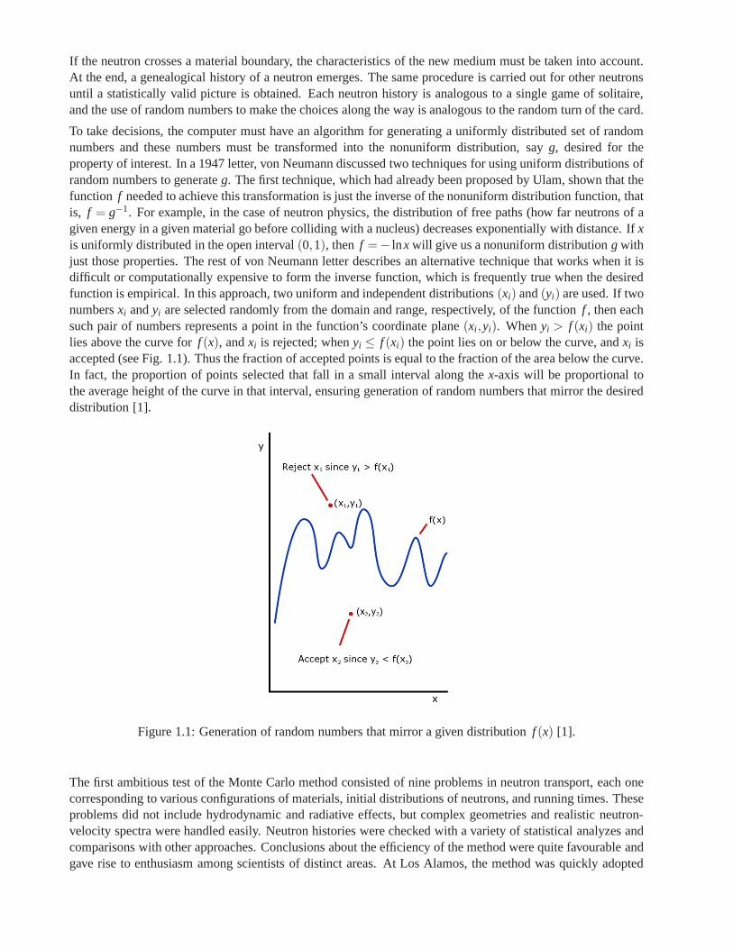
To take decisions, the computer must have an algorithm for generating a uniformly distributed set of randomnumbers and these numbers must be transformed into the nonuniform distribution, sayg, desired for theproperty of interest. In a 1947 letter, von Neumann discussed two techniques for using uniform distributions ofrandom numbers to generateg. The first technique, which had already been proposed by Ulam, shown that thefunction f needed to achieve this transformation is just the inverse ofthe nonuniform distribution function, thatis, f = g−1. For example, in the case of neutron physics, the distribution of free paths (how far neutrons of agiven energy in a given material go before colliding with a nucleus) decreases exponentially with distance. Ifxis uniformly distributed in the open interval(0,1), then f =− lnx will give us a nonuniform distributiong withjust those properties. The rest of von Neumann letter describes an alternative technique that works when it isdifficult or computationally expensive to form the inverse function, which is frequently true when the desiredfunction is empirical. In this approach, two uniform and independent distributions(xi) and(yi) are used. If twonumbersxi andyi are selected randomly from the domain and range, respectively, of the function f , then eachsuch pair of numbers represents a point in the function’s coordinate plane(xi ,yi). Whenyi > f (xi) the pointlies above the curve forf (x), andxi is rejected; whenyi ≤ f (xi) the point lies on or below the curve, andxi isaccepted (see Fig. 1.1). Thus the fraction of accepted points is equal to the fraction of the area below the curve.In fact, the proportion of points selected that fall in a small interval along thex-axis will be proportional tothe average height of the curve in that interval, ensuring generation of random numbers that mirror the desireddistribution [1].
Figure 1.1: Generation of random numbers that mirror a givendistribution f (x) [1].
The first ambitious test of the Monte Carlo method consisted of nine problems in neutron transport, each onecorresponding to various configurations of materials, initial distributions of neutrons, and running times. Theseproblems did not include hydrodynamic and radiative effects, but complex geometries and realistic neutron-velocity spectra were handled easily. Neutron histories were checked with a variety of statistical analyzes andcomparisons with other approaches. Conclusions about the efficiency of the method were quite favourable andgave rise to enthusiasm among scientists of distinct areas.At Los Alamos, the method was quickly adopted
to study problems of thermonuclear and fission devices. Already in 1948, Ulam was able to report to theAtomic Energy Commission about the applicability of the method for cosmic rays and in the area of theHamilton Jacobi partial differential equation. Other laboratory staff members started to run Monte Carlo codesin ENIAC. Among them, J. Calkin, C. Evans and F. Evans studiedthermonuclear problems, and B. Suydamand R. Stark tested the concept of artificial viscosity for time-dependent shocks. By midyear 1949, Ulam andMetropolis published a paper describing the Monte Carlo method and its application to integro-differentialequations [6] and the first symposium on the method was held inLos Angeles.
The construction of a new machine began later and N. Metropolis was the leader of the group in charge of it.He called the new machine MANIAC wishing to stop the use of acronyms for machine names, but contraryto what he sought, it only stimulated it. In early 1952, the MANIAC became operational at Los Alamos andsoon after, Anthony Turkevich led a study of the nuclear cascades resulting from the collision of acceleratedparticles with atomic nuclei. Another computational problem run on the MANIAC was a study of equations ofstate based on the two-dimensional motion of hard spheres. The results were published in a famous paper in1953 [7] and describes a strategy leading to greater computational efficiency for equilibrium systems obeyingthe Boltzmann distribution function. The idea developed inthat is that if a move of a particle in the systemcauses a decrease in the total energy, the new configuration should be accepted. On the other hand, if there isan increase in energy, the new configuration is accepted onlyif it passes through a game of chances biased bya Boltzmann factor, otherwise, the old configuration is kept.
Since then, the Monte Carlo method has been proved to be a verypowerful and useful tool. For example,deterministic methods for numerical integration of functions with many variables are very inefficient becausewith every additional dimension or variable, an exponential time increase takes place. The alternative wayprovided by the Monte Carlo method is the following: the function in question can be estimated by randomlyselecting points in the many dimensional space and taking some kind of average of the values of the function atthese points. This method will display 1/
√N convergence, i.e. quadrupling the number of sampled pointswill
halve the error, regardless of the number of dimensions. Theuse of Monte Carlo methods to model physicalproblems allows us to examine more complex systems that otherwise we are not able to handle. Solvingequations which describe the interactions between two atoms is fairly simple but solving the same equationsfor hundreds or thousands of atoms is impossible. With MonteCarlo methods, a large system can be sampledin a number of random configurations, and those data can be used to describe the system as a whole. There arecurrently many applications of the Monte Carlo method: stellar evolution [8], reactor design [9], cancer therapy[10], traffic flow [11], finance [12], simulations of various systems of interacting particles (e.g. ferromagneticmaterials), grain growth modeling in metallic alloys [13, 14], the behaviour of nanostructures and polymers[15], and protein structure predictions [16].
1.2 Basics of the Monte Carlo Method
In statistical mechanics, the partition functionZ(H,T) contains all the necessary information to calculate thethermodynamic properties of a system. The difficulty arise when the size of the system and the number ofdegrees of freedom for each particle is large, something that occurs in almost all cases. Then, summing overthe large number of possible states to calculateZ(H,T) is extremely expensive and almost impossible even ina computational way. The result is that, in general, the partition function can not be evaluated exactly [17].
The Monte Carlo approach consists of generating a series of possible states or configurationsX1,X2, ...,XN ofa system (Xi = {x1,x2...} with xi being the position of the particles in the system), so that the probabilityPXi
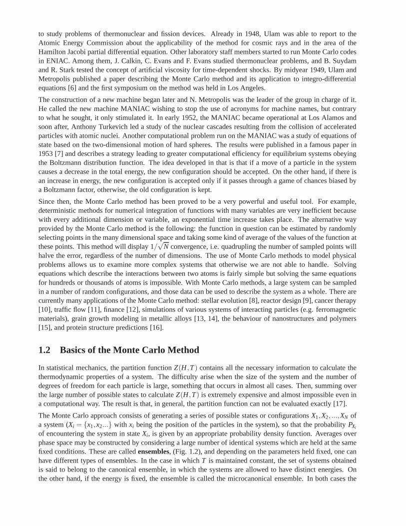
of encountering the system in stateXi, is given by an appropriate probability density function. Averages overphase space may be constructed by considering a large numberof identical systems which are held at the samefixed conditions. These are calledensembles, (Fig. 1.2), and depending on the parameters held fixed, one canhave different types of ensembles. In the case in whichT is maintained constant, the set of systems obtainedis said to belong to the canonical ensemble, in which the systems are allowed to have distinct energies. Onthe other hand, if the energy is fixed, the ensemble is called the microcanonical ensemble. In both cases the
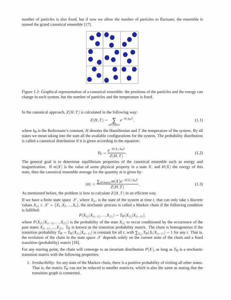
number of particles is also fixed, but if now we allow the number of particles to fluctuate, the ensemble isnamed the grand canonical ensemble [17].
Figure 1.2: Graphical representation of a canonical ensemble: the positions of the particles and the energy canchange in each system, but the number of particles and the temperature is fixed.
In the canonical approach,Z(H,T) is calculated in the following way:
Z(H,T) = ∑all states
e−H/kBT , (1.1)
wherekB is the Boltzmann’s constant,H denotes the Hamiltonian andT the temperature of the system. By allstates we mean taking into the sum all the available configurations for the system. The probability distributionis called a canonical distribution if it is given according to the equation:
PX =e−H(X)/kBT
Z(H,T). (1.2)
The general goal is to determine equilibrium properties of the canonical ensemble such as energy andmagnetization. Ifm(X) is the value of some physical property in a stateX, andH(X) the energy of thisstate, then the canonical ensemble average for the quantitym is given by:
〈m〉= ∑all statesm(X)e−H(X)/kBT
Z(H,T). (1.3)
As mentioned before, the problem is how to calculateZ(H,T) in an efficient way.
If we have a finite state spaceX , whereX(t) is the state of the system at timet, that can only takes discretevaluesX(i) ∈ X = {X1,X2, ...,Xs}, the stochastic process is called a Markov chain if the following conditionis fulfilled:
P(X(t)|X(t−1), ...,X(1)) = TM(X(t)|X(t−1)),
whereP(X(t)|X(t−1), ...,X(1)) is the probability of the stateX(t) to occur conditioned by the occurrence of thepast statesX(t−1), ...,X(1). TM is known as the transition probability matrix. The chain is homogeneous if thetransition probabilityTM = TM(X(t)|X(t−1)) is constant for allt, with ∑X(t)
TM(Xt |X(t−1)) = 1 for anyt. That is,the evolution of the chain in the state spaceX depends solely on the current state of the chain and a fixedtransition (probability) matrix [18].
For any starting point, the chain will converge to an invariant distributionP(X), as long asTM is a stochastictransition matrix with the following properties:
1. Irreducibility: for any state of the Markov chain, there is a positive probability of visiting all other states.That is, the matrixTM can not be reduced to smaller matrices, which is also the sameas stating that thetransition graph is connected.
2. Aperiodicity: the chain should not get trapped in cycles [18], i.e., the system should not be limited to asubchain of states.
Consider now a large collection of copies of the same system in equilibrium. We allow each copy to evolve intime and, at any instant, we will find each different copy in one possible configuration, an all the copies willgive a probability distribution over the configuration space. For each pointXi in the configuration space, theprobabilityP of finding a copy inX at timet satisfies the equation:
ddt
P(X, t) = ∑i
[P(Xi, t)TM(Xi → X)−P(X, t)TM(X → Xi)]. (1.4)
TM(X → Xi) andTM(Xi → X) are the probabilities of making a transition from the configuration X to Xi andviceversa. Because the collection is in equilibrium, the probability distribution is time invariant, and in the lastequation we must havedP(X, t)/dt = 0 for all t. At any instant, there is an equal number of transitions to andfrom the configurationX. In fact, there exists an equation like (1.4) for each point in the configuration space,and the set of all such equations forms the master equation [19].
A sufficient (but not necessary) condition for an equilibrium (time independent) probability distribution neededto simulate equilibrium systems is the so-calleddetailed balance conditionfor the master equation that relatesthe transition between two configurations,Xn−1 andXn through:
P(Xn)TM(X(n−1)|X(n)) = P(X(n−1))TM(X(n)|X(n−1)). (1.5)
This method can be used for any probability distribution of configurations. If we choose the Boltzmanndistribution, for which the probability of finding a configuration X with energyH at equilibrium is givenby (1.2), and substitute it into (1.5), we get:
TM(X(n−1)|X(n))
TM(X(n)|X(n−1))=
e−H(n−1)/kBT
e−H(n)/kBT= e∆E/kBT . (1.6)
This is the detailed balance condition on the transition probabilities. It is very important to note thatZ(H,T)does not appear in this expression; it only involves quantities that we know(kBT) or that can be easilycalculated(E).
Thus, we have a valid Monte Carlo algorithm if we generate a new configurationX(n) from a previous oneX(n−1) such that the transition probability satisfies the detailedbalance condition, and the generation procedureis ergodic, i.e. every configuration can be reached from every other configuration in a finite number of iterations[20].
1.3 Measurements Using the Monte Carlo Method
Systems generated using a valid Monte Carlo algorithm are often held at fixed values of intensive variables,such as temperature, pressure, and so on. The correspondingconjugate extensive variables (energy, volume,etc.) will fluctuate in time; indeed these fluctuations will actually be observed during the Monte Carlosimulations and will help us to measure quantities of interest such as:
Specific heat
CV =1V
(
∂E∂T
)
V= 〈(E−〈E〉)2〉= 〈E2〉− 〈E〉2. (1.7)
Susceptibility
χ =1V
(
∂M∂T
)
V= 〈(M−〈M〉)2〉= 〈M2〉− 〈M〉2. (1.8)
These and other similar quantities are measured for each configuration and the averages and statistical errorscalculated [17].
Summarizing, the idea of Monte Carlo simulations is to create an independently and identically distributed setof N samples from a target densityP(X) distribution function defined on a high dimensional state spaceX
(e.g., the set of possible configurations of a system). TheseN samples can be used to approximateP(X) [18].
WhenP(X) has a standard form, e.g., Gaussian, it is straightforward to sample from it using easily availableroutines. However, when this is not the case, we need to introduce more sophisticated techniques such asMarkov Chain Monte Carlo (MCMC) briefly presented above, which is a strategy of generating samples usinga Markov chain mechanism while exploring the state spaceX . This mechanism is constructed with thecondition that the chain spends more time in the most important regions. In particular, it is constructed so thatthe samples mimic samples drawn from the target density distribution P(X) [18].
1.4 Ising and Potts Models
The Ising model was proposed in 1925, in the doctoral thesis of Ernst Ising, a student of Wilhelm Lenz [21].Using a model proposed by Lenz in 1920 [22], Ising tried to explain certain empirically observed facts aboutferromagnetic materials in his thesis. The model was referred to in a paper by Heisenberg of 1928 in whichhe used the exchange mechanism to describe ferromagnetism [23]. After the publication of a paper by Peierls(1936) [24], in which he gave a non-rigorous proof that spontaneous magnetization must exist, the Ising modelbecame a well-established paradigm. In 1941, Kramers and Wannier calculated the Curie temperature using atwo-dimensional Ising model [25] and three years later Onsager gave a complete analytic solution of the model[26].
As a paradigm of statistical mechanics, the Ising model tries to imitate systems in which individual elements(e.g., atoms, animals, protein folds, biological membrane, social behaviour, etc.) modify their behaviour so asto conform to the dynamics of other elements in their neighbourhood [27].
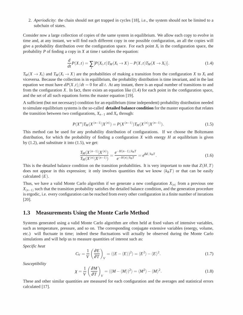
In most specific terms, the Ising model in statistical mechanics considers a system with spins located at thesites of a D-dimensional lattice, where each spin can take the value +1, corresponding to spin up, or the value-1, corresponding to spin down. The Hamiltonian of such a spin lattice system is given by:
HI =−J ∑〈i, j〉
σiσ j −B∑i
σi , (1.9)
whereJ is the exchange constant, andσi andσ j are the spins of theith and jth sites respectively. The sites areusually a pair of nearest neighbours, though calculations for more distant neighbours can also be carried out.B is an externally applied magnetic field with whom each spin interacts.
Figure 1.3: Lattice representations of Ising and Potts models. The red site interacts with his first neighbours(in yellow). Notice that in the Potts model, being a generalization of the Ising model, more than two possibledirections for the spin are available.

WhenJ > 0, the model describes a ferromagnetic system where parallel spins are favoured and antiparallelspins are discouraged.
In the case ofJ < 0, an antiferromagnetic system is modeled.
If J is randomly chosen to be 1 or -1 for each pair of nearest neighbours and remain fixed during the course ofobservation, we obtain a model of a spin glass [28].
The energy associated with each state depends then on the exchange energy of the particles and the interactionof the particles with the external magnetic field. However, in the absence of the external field, the energy ofthe system depends only on the spin exchange energy:
HI =−J ∑〈i, j〉
σiσ j . (1.10)
The Potts model is a generalization of the Ising model, in which spins can choose its value from a discrete setof states (see Fig. 1.3). In 1952, C. Domb proposed it as a doctoral thesis for his student R. Potts [29]. Withoutthe presence of an external field the Potts model is defined through the Hamiltonian:
HP =−J ∑〈i, j〉
δσi ,σ j σiσ j , (1.11)
whereJ denotes again the interaction exchange constant between nearest neighbours and the valuesσi arecharacterized by an integerσi = 1,2, ...,q. If two spins are parallel they contribute with energyJ, otherwisetheir energy contribution is null.
1.5 Some Monte Carlo Algorithms: Metropolis, Swendsen-Wang and Wolff
The Metropolis [7], Swendsen-Wang [30] and Wolff [31] algorithms satisfy the master equation and thedetailed balance condition for the Boltzmann distribution. Consequently, when the system reaches equilibrium,the probability distribution of all possible configurations will be the Boltzmann distribution.
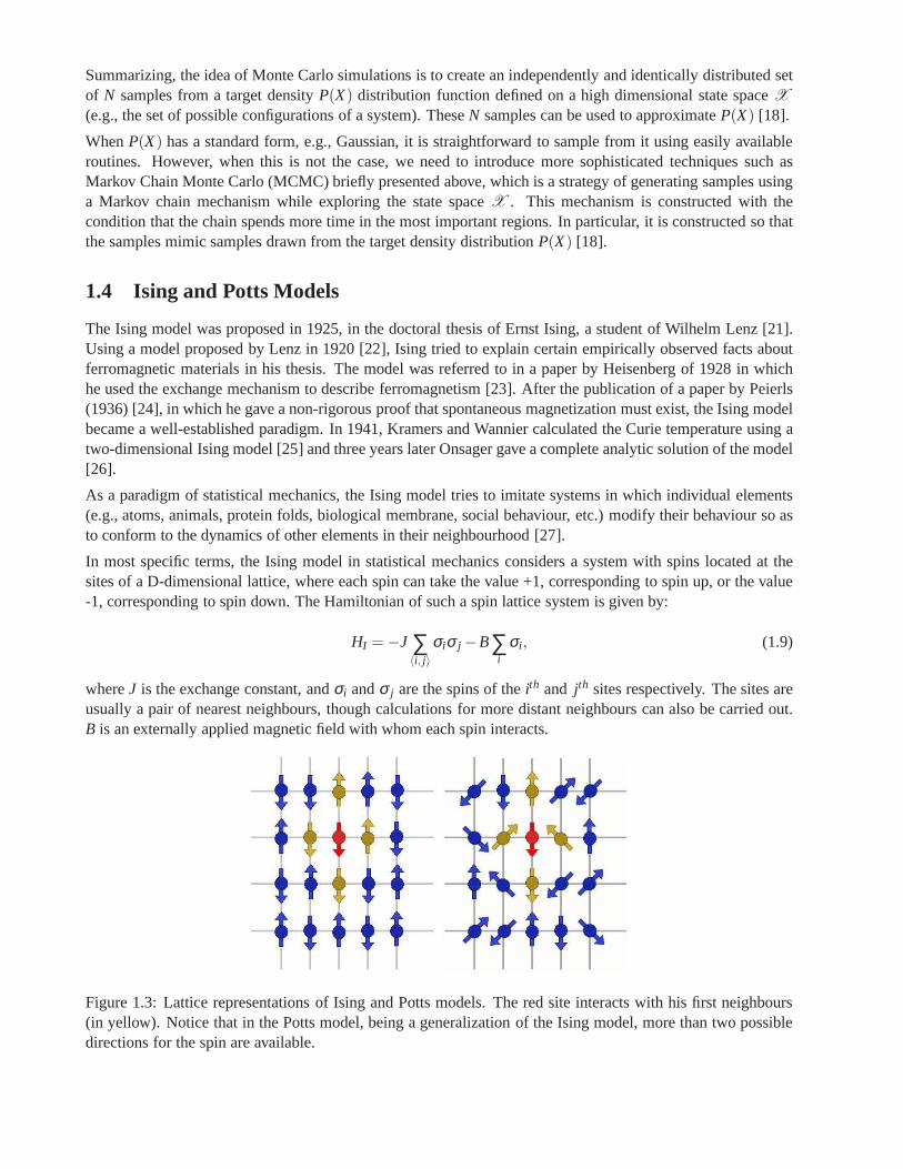
The steps of the Metropolis algorithm for an Ising model are graphically represented in Fig. 1.7 and are thefollowing:
1. Start with an arbitrary spin configurationC0 of a lattice withN sites.
2. Select a spin randomly and independently, and flip it.
3. Calculate the energy change∆E which results if the spin is turned.
4. Generate a random numberr such that 0< r < 1.
5. If ∆E ≤ 0, accept the change; if∆E > 0, the configuration is accepted with a probabilitye−∆E/kBT . Thisis resumed as: ifr < e−∆E/kBT the spin is flipped. If not, the new configuration is rejected,and the systemreturns to the initial configurationC0.
6. Choose randomly another spin to flip and go to (3).
It is important to discard some configurations at the beginning of the chain of configurations to ensure thatthe system forgetsC0 and that the configurations taken into account form a canonical ensemble. Then, aftera considerable number of spins have been updated, the properties of the system are determined and added tothe statistical average which is stored. The random numberr must be chosen uniformly in the interval[0,1]and all the successive random numbers should be uncorrelated. Note that if a spin trial is rejected, the oldstate is counted again for the averages. For aq state Potts model, the new value for the chosen spin is selectedrandomly among the otherq−1 spin values [17].
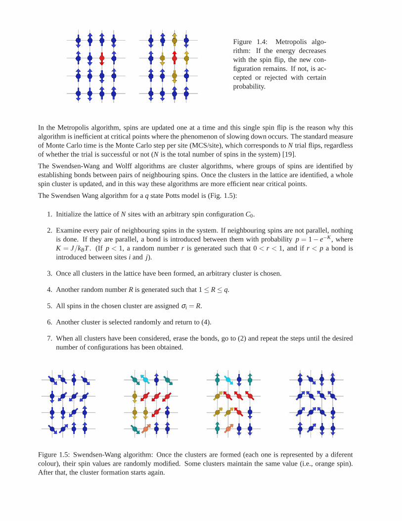
Figure 1.4: Metropolis algo-rithm: If the energy decreaseswith the spin flip, the new con-figuration remains. If not, is ac-cepted or rejected with certainprobability.
In the Metropolis algorithm, spins are updated one at a time and this single spin flip is the reason why thisalgorithm is inefficient at critical points where the phenomenon of slowing down occurs. The standard measureof Monte Carlo time is the Monte Carlo step per site (MCS/site), which corresponds toN trial flips, regardlessof whether the trial is successful or not (N is the total number of spins in the system) [19].
The Swendsen-Wang and Wolff algorithms are cluster algorithms, where groups of spins are identified byestablishing bonds between pairs of neighbouring spins. Once the clusters in the lattice are identified, a wholespin cluster is updated, and in this way these algorithms aremore efficient near critical points.
The Swendsen Wang algorithm for aq state Potts model is (Fig. 1.5):
1. Initialize the lattice ofN sites with an arbitrary spin configurationC0.
2. Examine every pair of neighbouring spins in the system. Ifneighbouring spins are not parallel, nothingis done. If they are parallel, a bond is introduced between them with probabilityp = 1− e−K , whereK = J/kBT. (If p < 1, a random numberr is generated such that 0< r < 1, and if r < p a bond isintroduced between sitesi and j).
3. Once all clusters in the lattice have been formed, an arbitrary cluster is chosen.
4. Another random numberR is generated such that 1≤ R≤ q.
5. All spins in the chosen cluster are assignedσi = R.
6. Another cluster is selected randomly and return to (4).
7. When all clusters have been considered, erase the bonds, go to (2) and repeat the steps until the desirednumber of configurations has been obtained.
Figure 1.5: Swendsen-Wang algorithm: Once the clusters areformed (each one is represented by a diferentcolour), their spin values are randomly modified. Some clusters maintain the same value (i.e., orange spin).After that, the cluster formation starts again.
One Monte Carlo cycle in the Swendsen-Wang algorithm is accomplished when all clusters have been updated(steps 2-6), and is equivalent to one Monte Carlo step per site (MCS/site) in the Metropolis algorithm [19].
The probability to set a bond between two sites depends on thetemperature, which affects the resultant clusterdistribution. At very high temperature, the clusters will tend to be quite small, whereas at very low temperaturevirtually all sites with nearest neighbours in the same state will belong to the same cluster and therefore therewill be a tendency for the system to oscillate back and forth between quite structures. However, near a criticalpoint, a quite rich array of clusters is produced and the net result is that each configuration differs substantiallyfrom its previous one. That is the main reason why the critical slowing down is reduced [17].
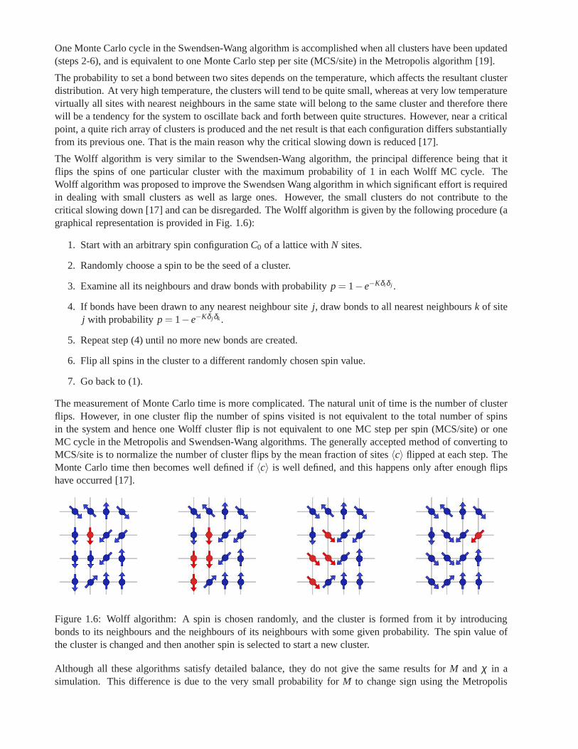
The Wolff algorithm is very similar to the Swendsen-Wang algorithm, the principal difference being that itflips the spins of one particular cluster with the maximum probability of 1 in each Wolff MC cycle. TheWolff algorithm was proposed to improve the Swendsen Wang algorithm in which significant effort is requiredin dealing with small clusters as well as large ones. However, the small clusters do not contribute to thecritical slowing down [17] and can be disregarded. The Wolffalgorithm is given by the following procedure (agraphical representation is provided in Fig. 1.6):
1. Start with an arbitrary spin configurationC0 of a lattice withN sites.
2. Randomly choose a spin to be the seed of a cluster.
3. Examine all its neighbours and draw bonds with probability p= 1−e−Kδi δ j .
4. If bonds have been drawn to any nearest neighbour sitej, draw bonds to all nearest neighboursk of sitej with probability p= 1−e−Kδ j δk.
5. Repeat step (4) until no more new bonds are created.
6. Flip all spins in the cluster to a different randomly chosen spin value.
7. Go back to (1).
The measurement of Monte Carlo time is more complicated. Thenatural unit of time is the number of clusterflips. However, in one cluster flip the number of spins visitedis not equivalent to the total number of spinsin the system and hence one Wolff cluster flip is not equivalent to one MC step per spin (MCS/site) or oneMC cycle in the Metropolis and Swendsen-Wang algorithms. The generally accepted method of converting toMCS/site is to normalize the number of cluster flips by the mean fraction of sites〈c〉 flipped at each step. TheMonte Carlo time then becomes well defined if〈c〉 is well defined, and this happens only after enough flipshave occurred [17].
Figure 1.6: Wolff algorithm: A spin is chosen randomly, and the cluster is formed from it by introducingbonds to its neighbours and the neighbours of its neighbourswith some given probability. The spin value ofthe cluster is changed and then another spin is selected to start a new cluster.
Although all these algorithms satisfy detailed balance, they do not give the same results forM and χ in asimulation. This difference is due to the very small probability for M to change sign using the Metropolis
algorithm for large systems, at low temperatures. This corresponds to a physical situation, and one cancalculate〈M〉 andχ and obtain meaningful results. However in cluster algorithms, the clusters become verylarge at low temperatures, and by flipping them, we effectively flip the whole system, yielding〈M〉 = 0; thevariance inM is then simply〈M2〉, a constant at low temperatures, which in turn gives a diverging χM asT → 0. The solution is to use|M| instead ofM, and defineχ|M| just as we definedχ earlier. In this way, allthree algorithms give the same results for〈M〉 andχ|M| at all temperatures [19].
Notice that cluster algorithms become inefficient at low temperatures, because in that situation, nearly allspins in the system are flipped when we flip the largest cluster, which is not helpful in achieving statisticallyindependent configurations. In comparison, the Metropolisalgorithm will be much more efficient [19].
Once an appropiate algorithm has been selected, one of the goals of Monte Carlo simulations is the study ofthe behaviour of systems in phase transitions.
1.6 Phase Transitions and Critical Exponents
One of the most common physical problems studied in simulations are phase transitions. A phase transitionoccurs when a thermodynamic system passes from one phase to another one with the change of some externalvariable, such as temperature or pressure. Some examples are the transitions between solid, liquid, and gaseousphases, the transition between the ferromagnetic and paramagnetic phases of magnetic materials, and theemergence superconductivity in certain metals when they are cooled below a critical temperature [32].
When a system goes from one phase to another, there will be in general a stage where the free energy is notanalytic. Due to this, the free energies on either side of thetransition are two different functions, so one ormore thermodynamic properties will behave very differently after the transition. A system near or at the criticalpoint of a phase transition presents peculiar behaviours that are universal, like divergence of some quantitiesand critical slowing down phenomena, which will be explained later. The most commonly examined propertyin this context is the heat capacity that in the transition region may become infinite, jump abruptly to a differentvalue, or exhibit a discontinuity in its derivative [33]. This non-analytic behaviour stems generally from theinteractions of an extremely large number of particles in a system, and does not show up with the same strengthin systems that are too small [32].
Phase transitions are generally classified into first or second order transitions. A second order, or continuousphase transition, can be defined as a point at which a system changes from one state to another one without adiscontinuity or jump in its density, internal energy, magnetization, or similar properties. In the case of a firstorder transition, the above mentioned properties jump discontinuously as the temperature or pressure passesthrough the transition point [34]. The name of different kind of phase transitions comes precisely from thenumber of derivatives of the free energy that we have to countbefore we can see a discontinuous behaviour. Ifthe first derivative is discontinuous, we have a first order transition, if not, it is a second order one [17].The first-order phase transitions involve a latent heat. During such transition, a system either absorbs or releasesa fixed (typically large) amount of energy. Because energy can not be instantaneously transferred between thesystem and its environment, first-order transitions are associated with “mixed-phase regimes” in which someparts of the system have completed the transition and othershave not. Continuous phase transitions, in manycases, are associated with a change of symmetry of the systemand are easier to study than first-order transitionsdue to the absence of latent heat. They have shown many interesting properties. The phenomena associatedwith continuous phase transitions are called critical phenomena, because of their occurrence near critical pointsand because it turns out that continuous phase transitions can be characterized by parameters known as criticalexponents [32].
In the case of many phase transitions a non-zero value of an order parameter appears, i.e., some property of thesystem which is non zero in one phase (usually called the ordered phase) but identically zero in the other phase(disordered phase). Thus, the order parameter can not be an analytic function at the transition point. The orderparameter is defined differently in various kinds of physical systems [17]. For systems such as the ferromagnet,
where there is a broken symmetry below critical temperatureTc, the order parameter is the magnetization. Forsystems without broken symmetry, one chooses some quantitythat is very sensitive to the difference betweenthe two phases, and measures the difference of this quantityfrom its value at the critical point and below it.For the liquid-vapor critical point, we may choose the orderparameter as the difference between the actualdensity of the fluid and the density at the critical point. Forliquid crystals the degree of orientational order isconsidered as the order parameter [34].
Another quantity of interest near a phase transition is the correlation function. In general, there will bemicroscopic regions in which the characteristics of the material are correlated. This is generally measuredthrough the determination of atwo point correlation function, which is the probability of finding that two sitesseparated by a distancer have the same value of a certain given quantityρ [17]:
Γρ(r) = 〈ρ(0)ρ(r)〉. (1.12)
In the case of magnetic systems, the correlation function can be measured in neutron scattering experiments,whereas near the liquid vapour transition it can be measuredby light scattering or small angle X-ray-scatteringexperiments [34].
If the correlation for the appropriate quantity decays to zero as the distance goes to infinity, then the orderparameter is zero [17]. Close to the critical point, the correlation lengthξ , which tells us how far correlationsare still present, becomes extremely large. This is directly related to the large amount of long-wavelengthfluctuations that occur in the system at the criticality [34]. The time taken for the system to changeconfiguration near the critical point also increase significantly because of the divergence of the correlationlength ξ . This phenomenon is called critical slowing down. For example, in the case of the Ising model,spins tend to align with their neighbours due to the exchangeinteraction, and regions or clusters of spinspointing in the same direction appear. These spins are said to be correlated, and, generally, there are clustersof various sizes. The span of the largest one is the correlation lengthξ , while the time it takes to break up theexisting conformation of spins and form another arrangement of clusters is called the decorrelation timeτ . Atthe critical point, there is a low probability for a spin in the middle of a spin cluster to change its direction,therefore spin regions are altered only at the boundary. This gives rise to a long decorrelation time which isrelated to the correlation length by a power law:
τ ∝ ξ z, (1.13)
wherez is the dynamical critical exponent [19]. For simulations ofa finite lattice of linear dimensionL, ξ isnaturally bounded byL and then the basic assumption is that:
τ ∝ Lz. (1.14)
These two equations describe the critical slowing down. In an infinite system, as the critical point isapproached, the correlation length diverges (its value is∞), and from (1.13), we see that the decorrelationtime also diverges. In finite systemsξ does not diverge as the critical point is approached, however, it reachesits peak with a sharp slope. Due to the power law dependence ofτ onξ , τ will also display a peak with a sharpslope, exhibiting critical slowing down [19].
Near the transition points, the critical slowing down phenomenon produces important effects that complicatethe implementation of the Monte Carlo method. This is the main reason why the scientists introducedalternative approaches besides canonical Metropolis algorithm, such as Wolff and Swendsen-Wang algorithms.The computational effect of critical slowing down near a critical point can be understood in the followingmanner: when we simulate finite systems at the critical point, the decorrelation time depends on the lineardimensionL through a power law asL approaches infinity. Take, for example, the 2D Ising model. Thedynamical critical exponentz is known to be approximately 2 using the Metropolis algorithm. If the time ittakes to obtain 100 statistically independent configurations ist in a system withL = 32, then ifL is increasedby a factor of 2 to 64, the computational time needed to obtain100 statistically independent configurations will
increase to 42 t. A factor of 4 is introduced because the number of spins is increased by 4, and another factorof 4 is due to the fact thatτ ∝ L2. In general, the amount of CPU time required to obtain a fixed number ofstatistically independent configurations for a system withlinear dimensionL is proportional toLd+z, wheredis the spatial dimension of the model, andz is the corresponding dynamical critical exponent [19].
Data from experiments, as well as results for a number of exactly solvable models, show that in the vicinity ofthe critical pointTc, the thermodynamical properties can be described by a set ofsimple power laws [17]. Forexample, for the determination of the way which the magnitude of the order parameter approaches zero as thecritical point is reached, we may write (according to the classical theories of phase transitions such as the vander Waals or mean field theories):
M = M0εβ , (1.15)
whereM is the order parameter (i.e., the magnetization for a ferromagnet),M0 is a constant that will vary fromone system to another,ε = |1−T/Tc|, and the exponentβ is called critical exponent [34].
The temperature variation of the order parameter is very important but not the only quantity of interest. Anotherkey quantity is the specific heat, defined as the derivative ofthe internal energy with respect to the temperature.The specific heat is found to become infinite at the critical point in some systems but also one can have casesin which the specific heat is finite with only a sharp cusplike maximum at the critical point [34]. In either case,one may define an exponentα that characterizes the anomalous behaviour of the specific heat at the criticalpoint:
CV =C0ε−α . (1.16)
Susceptibilityχ is another quantity of interest. It is defined as the derivative of the order parameter with respectto the applied field to which it is coupled, under constant temperature condition. For a magnetic system, thisquantity is precisely the magnetic susceptibility. This quantity becomes extremely large near the critical point,and we may write the zero field magnetic susceptibility as [34]:
χ = χ0 ε−γ . (1.17)
Finally, the correlation lengthξ varies as:
ξ = ξ0 ε−ν , (1.18)
where, again,ν is termed as critical exponent.
Note that the last equations represent asymptotic expressions which are only valid ifε → 0 and more completeforms would include additional corrections to scaling terms which describe the deviations from the asymptoticbehaviour. The exact values of these critical exponents areknown exactly only for a small number of models,most notably for the 2D Ising square lattice [26], whose exact solution shows thatα = 0, β = 1/8, andγ = 7/4.Here,α = 0 corresponds to a logarithmic divergence of the specific heat [17].
The power law behaviour near critical points is very generaland many systems share the same criticalexponents. In particular, the Ising universality class refers to the class of critical phenomena that share thesame critical exponents as the Ising model [19].
Although the critical exponents,α , β , andγ defined above may be independent in principle, they were foundempirically, in the 1960’s, to be connected by the relationship:
α = 2− γ −2β . (1.19)
This equality is known as the Rushbrooke relation, and the following three relations are also known [17], whereη andδ are two additional critical exponents:
Josephson: νD = 2−α ,Widom: γ = β (δ −1) ,Fisher: γ = ν(2−η) .
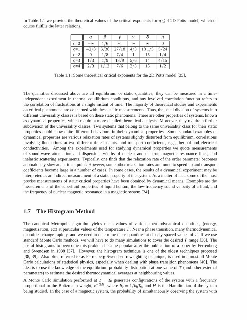
In Table 1.1 we provide the theoretical values of the critical exponents forq ≤ 4 2D Potts model, which ofcourse fulfills the latter relations.
α β γ ν δ ηq=0 −∞ 1/6 ∞ ∞ ∞ 0q=1 −2/3 5/36 27/18 4/3 18 1/5 5/24q=2 0 1/8 7/4 1 15 1/4q=3 1/3 1/9 13/9 5/6 14 4/15q=4 2/3 1/12 7/6 2/3 15 1/2
Table 1.1: Some theoretical critical exponents for the 2D Potts model [35].
The quantities discussed above are all equilibrium or static quantities; they can be measured in a time-independent experiment in thermal equilibrium conditions, and any involved correlation function refers tothe correlation of fluctuations at a single instant of time. The majority of theoretical studies and experimentson critical phenomena are concerned with these static measurements. Thus, the usual division of systems intodifferent universality classes is based on these static phenomena. There are other properties of systems, knownas dynamical properties, which require a more detailed theoretical analysis. Moreover, they require a furthersubdivision of the universality classes. Two systems that belong to the same universality class for their staticproperties could show quite different behaviours in their dynamical properties. Some standard examples ofdynamical properties are various relaxation rates of systems slightly disturbed from equilibrium, correlationsinvolving fluctuations at two different time instants, and transport coefficients, e.g., thermal and electricalconductivities. Among the experiments used for studying dynamical properties we quote measurementsof sound-wave attenuation and dispersion, widths of nuclear and electron magnetic resonance lines, andinelastic scattering experiments. Typically, one finds that the relaxation rate of the order parameter becomesanomalously slow at a critical point. However, some other relaxation rates are found to speed up and transportcoefficients become large in a number of cases. In some cases,the results of a dynamical experiment may beinterpreted as an indirect measurement of a static propertyof the system. As a matter of fact, some of the mostprecise measurements of static critical properties have been obtained by dynamical means. Examples are themeasurements of the superfluid properties of liquid helium,the low-frequency sound velocity of a fluid, andthe frequency of nuclear magnetic resonance in a magnetic system [34].
1.7 The Histogram Method
The canonical Metropolis algorithm yields mean values of various thermodynamical quantities, (energy,magnetization, etc) at particular values of the temperature T. Near a phase transition, many thermodynamicalquantities change rapidly, and we need to determine these quantities at closely spaced values ofT. If we usestandard Monte Carlo methods, we will have to do many simulations to cover the desiredT range [36]. Theuse of histograms to overcome this problem became popular after the publication of a paper by Ferrenbergand Swendsen in 1988 [37]. However, the histogram techniqueis one of the oldest techniques proposed[38, 39]. Also often referred to as Ferrenberg-Swendsen reweighting technique, is used in almost all MonteCarlo calculations of statistical physics, especially when dealing with phase transition phenomena [40]. Theidea is to use the knowledge of the equilibrium probability distribution at one value ofT (and other externalparameters) to estimate the desired thermodynamical averages at neighbouring values.
A Monte Carlo simulation performed atT = T0 generates configurations of the system with a frequencyproportional to the Boltzmann weight,e−β0H , whereβ0 = 1/kBT0, andH is the Hamiltonian of the systembeing studied. In the case of a magnetic system, the probability of simultaneously observing the system with
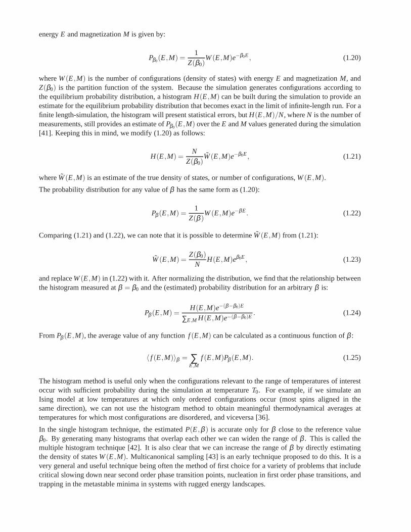
energyE and magnetizationM is given by:
Pβ0(E,M) =
1Z(β0)
W(E,M)e−β0E, (1.20)
whereW(E,M) is the number of configurations (density of states) with energy E and magnetizationM, andZ(β0) is the partition function of the system. Because the simulation generates configurations according tothe equilibrium probability distribution, a histogramH(E,M) can be built during the simulation to provide anestimate for the equilibrium probability distribution that becomes exact in the limit of infinite-length run. For afinite length-simulation, the histogram will present statistical errors, butH(E,M)/N, whereN is the number ofmeasurements, still provides an estimate ofPβ0
(E,M) over theE andM values generated during the simulation[41]. Keeping this in mind, we modify (1.20) as follows:
H(E,M) =N
Z(β0)W(E,M)e−β0E, (1.21)
whereW(E,M) is an estimate of the true density of states, or number of configurations,W(E,M).
The probability distribution for any value ofβ has the same form as (1.20):
Pβ (E,M) =1
Z(β )W(E,M)e−βE. (1.22)
Comparing (1.21) and (1.22), we can note that it is possible to determineW(E,M) from (1.21):
W(E,M) =Z(β0)
NH(E,M)eβ0E, (1.23)
and replaceW(E,M) in (1.22) with it. After normalizing the distribution, we find that the relationship betweenthe histogram measured atβ = β0 and the (estimated) probability distribution for an arbitrary β is:
Pβ (E,M) =H(E,M)e−(β−β0)E
∑E,M H(E,M)e−(β−β0)E. (1.24)
FromPβ (E,M), the average value of any functionf (E,M) can be calculated as a continuous function ofβ :
〈 f (E,M)〉β = ∑E,M
f (E,M)Pβ (E,M). (1.25)
The histogram method is useful only when the configurations relevant to the range of temperatures of interestoccur with sufficient probability during the simulation at temperatureT0. For example, if we simulate anIsing model at low temperatures at which only ordered configurations occur (most spins aligned in thesame direction), we can not use the histogram method to obtain meaningful thermodynamical averages attemperatures for which most configurations are disordered,and viceversa [36].
In the single histogram technique, the estimatedP(E,β ) is accurate only forβ close to the reference valueβ0. By generating many histograms that overlap each other we can widen the range ofβ . This is called themultiple histogram technique [42]. It is also clear that we can increase the range ofβ by directly estimatingthe density of statesW(E,M). Multicanonical sampling [43] is an early technique proposed to do this. It is avery general and useful technique being often the method of first choice for a variety of problems that includecritical slowing down near second order phase transition points, nucleation in first order phase transitions, andtrapping in the metastable minima in systems with rugged energy landscapes.
1.8 Identifying the Nature of Transitions and Finite Size Scaling
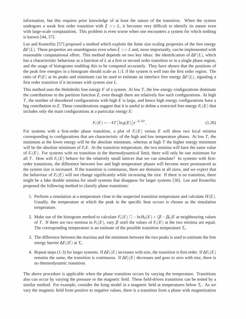
The behaviour near phase transitions has been one of the mainobjectives of studies focusing on the propertiesof physical systems but a correlation lengthξ greater than the accessible sizeL of the system may lead tomany difficulties [44]. For systems close to a second order phase transition, finite-size scaling is routinelyused to extract thermodynamic information from similar systems of fairly small size. An equivalent theory forfirst order phase transitions is clearly also of interest. A useful theory of finite-size scaling should allow us toextract the couplings at which the transition occurs, as well as other dimensional quantities like latent heat (orspontaneous magnetization) and specific heat (or magnetic susceptibility) [45].
First order transitions are characterized by a discontinuity in the order parameter and thermodynamicquantities, with an associated delta-peak behaviour in thesusceptibility. As a matter of fact, the jump in theenergy density is equivalent to the latent heat. However, atfinite size, thermodynamic quantities becomecontinuous and rounded. Instead of delta function behaviour in susceptibility there is only a hump. Insimulations, this behaviour is visible only if the simulation time τs is larger than the decorrelation timeτat the transition point.τs is typically very large sinceτ ∝ e−σ2LD−1
, whereσ is the surface tension of theinterface between the low temperature and high temperaturephases [47]. It is the dimensionD that now playsthe key role rather than the critical exponents as in the caseof second order phase transitions [17].
At the transition temperature of a first-order phase transition, a mixed state can exist where two different bulkphases are separated by an interface. The free energy densities of the two bulk phases are equal and the freeenergy of the mixed state is higher than any of the coexistingpure phases by an amountFs = σA, whereAis the area of the interface andσ is the interface tension [48]. In first order phase transitions, the correlationlength remains finite in both the ordered and disordered phases, i.e., the correlation length does not diverge.Thus, a different approach to finite size scaling must be used[17].
From fairly general arguments about the nature of discontinuities at a first-order phase transition, Fisher andBerker [49] obtained the infinite volume limit approached bymeasurements performed at finite volumes. Thisconventional scenario is based on a smooth behaviour of the renormalization group flow and the existence of adiscontinuity fixed point whose attraction domain containsthe transition surface and has relevant exponents ofthe formy= D [49]. The singularities associated with first order transitions are generated by infinite iterationsof renormalization group transformations in the thermodynamic limit. Correction terms were later calculated ina particular phenomenological model called the double-Gaussian model, in which the peaks in the probabilitydistribution for the coexisting phases were approximated by Gaussians [50, 51]. This model correctly predictsthe first term in a series of corrections in inverse powers of the volumeV, around the leading term obtained byFisher and Berker [49].
More recent developments are due to Borgs, Kotecký and Miracle-Solé [52, 53]. The basic idea is todecompose the partition function into a sum of the contributions, each due to one of the coexisting phases, andto neglect contributions due to phase mixtures. Each of these contributions to the total partition function thenyield quantities related to free energies in the pure phases. The analysis proceeds by power series expansionsof these partial partition functions around the phase transition point, leading to moments expressed in inversepowers of the volume [45]. According to this theory, for periodic boundary conditions, the specific heats andBinder cumulants at the transition temperature can be represented by polynomials in 1/LD. If the L >> ξ ,the contribution of the higher order terms are negligible [54, 55]. The difficulty arises whenξ ≥ L. In thiscase, higher order corrections are necessary and deciding the order of the transition becomes difficult. Evenwhen large lattices are used, higher order terms may create difficulties during the fitting procedure to thesimulation data. Such difficulties may be reduced by choosing the quantities for which the correction termsplay less important role. A good example for such quantity isthe average energy measured at the infinite latticetransition point, which has exponentially small correction term enabling one to determine the infinite latticecritical point with great accuracy [53, 54, 56].
Finite size scaling ideas for first or second order transitions help to extract critical exponents and other
information, but this requires prior knowledge of at least the nature of the transition. When the systemundergoes a weak first order transition withξ >> L, it becomes very difficult to identify its nature evenwith large-scale computations. This problem is even worse when one encounters a system for which nothingis known [44, 57].
Lee and Kosterlitz [57] proposed a method which exploits thefinite size scaling properties of the free energy∆F(L). These properties are unambiguous even whenξ >> L and, more importantly, can be implemented withreasonable computational effort. This method depends on two key ideas: the identification of∆F(L), whichhas a characteristic behaviour as a function ofL at a first or second order transition or in a single phase region,and the usage of histograms enabling this to be computed accurately. They have shown that the positions ofthe peak free energies in a histogram should scale as 1/L if the system is well into the first order region. Theratio of P(E) at its peaks and minimum can be used to estimate an interface free energy∆F(L), signaling afirst order transition if it increases with system sizeL.
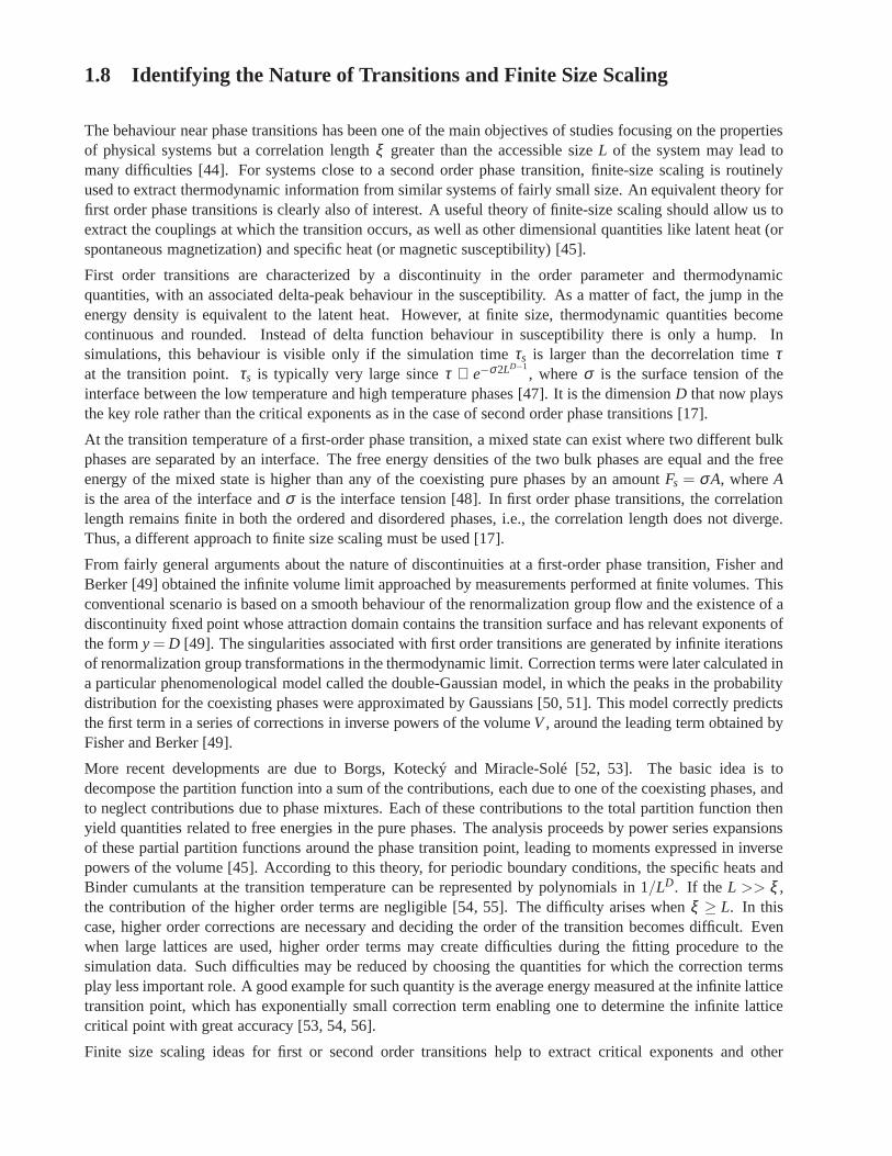
This method uses the Helmholtz free energyF of a system. At lowT, the low energy configurations dominatethe contributions to the partition functionZ, even though there are relatively few such configurations. At highT, the number of disordered configurations with highE is large, and hence high energy configurations have abig contribution toZ. These considerations suggest that it is useful to define a restricted free energyFr(E) thatincludes only the main configurations at a particular energyE:
Fr(E) =−kT[
lng(E)]
e−E/kT. (1.26)
For systems with a first-order phase transition, a plot ofFr(E) versusE will show two local minimacorresponding to configurations that are characteristic ofthe high and low temperature phases. At lowT, theminimum at the lower energy will be the absolute minimum, whereas at high T the higher energy minimumwill be the absolute minimum ofFrE. At the transition temperature, the two minima will have thesame valueof Fr(E). For systems with no transition in the thermodynamical limit, there will only be one minimum forall T. How will Fr(E) behave for the relatively small lattices that we can simulate? In systems with first-order transitions, the difference between low and high temperature phases will become more pronounced asthe system size is increased. If the transition is continuous, there are domains at all sizes, and we expect thatthe behaviour ofFr(E) will not change significantly while increasing the size. If there is no transition, theremight be a fake double minima for small systems that disappear for larger systems [36]. Lee and Kosterlitzproposed the following method to classify phase transitions:
1. Perform a simulation at a temperature close to the suspected transition temperature and calculateH(E).Usually, the temperature at which the peak in the specific heat occurs is chosen as the simulationtemperature.
2. Make use of the histogram method to calculateFr(E) ∝ − lnH0(E)+ (β −β0)E at neighbouring valuesof T. If there are two minima inFr(E), vary β until the values ofFr(E) at the two minima are equal.The corresponding temperature is an estimate of the possible transition temperatureTc.
3. The difference between the maxima and the minimum betweenthe two peaks is used to estimate the freeenergy barrier∆Fr(E) atTc.
4. Repeat steps (1-3) for larger systems. If∆Fr(E) increases with size, the transition is first order. If∆Fr(E)remains the same, the transition is continuous. If∆Fr(E) decreases and goes to zero with size, there isno thermodynamic transition.
The above procedure is applicable when the phase transitionoccurs by varying the temperature. Transitionsalso can occur by varying the pressure or the magnetic field. These field-driven transitions can be tested by asimilar method. For example, consider the Ising model in a magnetic field at temperatures belowTc. As wevary the magnetic field from positive to negative values, there is a transition from a phase with magnetization
M > 0 to a phase withM < 0. Is this a first-order or continuous transition? To answer this question, we canuse the Lee-Kosterlitz method with a histogramH(E,M) generated at zero magnetic field, and calculateFr(M)instead ofFr(E). The quantityFr(M) is proportional to− ln∑E H(E,M)e−(β−β0)E. Because the states withpositive and negative magnetization are equally likely to occur for zero magnetic field, we should see a doubleminima structure forFr(M) with equal minima. As we increase the size of the system,∆Fr should increase fora first order transition and remain the same for a continuous transition [36].
Another way to determine the nature of a first order phase transition is to use the Binder cumulant of energydefined by [58]:
UL = 1− 〈E4〉3〈E2〉2 . (1.27)
If various cumulants (each one corresponding to different lattice sizes) are plot in the same graph, a behaviourcharacteristic of a first order transition appears as will bediscussed in the next section.It can be shown that the minimum value ofUL is
UL,min =23− 1
3
(E2+−E2
−2E+E−
)2+O(L−d), (1.28)
whereE+ andE− are the energies of the two phases in a first order transition.These results are derived byconsidering the distribution of energy values to be a sum of Gaussians about each phase at the transition point,which become sharper and sharper asL → ∞ [36].
On the other hand, equations (1.15) to (1.18) for second order transitions are valid only for infinite systemsand, as a matter of fact, we can simulate only finite systems. Quantities that diverge in the infinite case nowpresent peaks in the finite system. Furthermore, the peaks occur at a valueTc(L), for a given linear dimensionL, slightly different from the infinite-lattice critical temperatureTc. However, at a second order phase change,the critical behaviour of a system in the thermodynamical limit can be extracted from the properties of finitesystems by examining the size dependence of the singular part of the free energy density. This finite sizescaling approach was first developed by Fisher [59]. According to his theory, the free energy of a system oflinear dimensionL is described by the scaling ansatz:
F(L,T,h) = L−(2−α)/νF0(tL1/ν , hL(γ+β)/ν), (1.29)
wheret = (T −Tc)/Tc, h is the magnetic field andF0 is a scaling function. The critical exponentsα , β , γ , andν all correspond to the values for the infinite system. Appropriate differentiation of the free energy yields thevarious thermodynamic properties with their corresponding scaling forms:
m= L−β/ν m0xt ,
C = Lα/ν C0 xt ,
χ = Lγ/ν χ0xt ,
(1.30)
wherext = tL1/ν is the temperature scaling variable [41].
To determine the transition temperature accurately one find the location of the peak in a thermodynamicderivative, for example, specific heat. For a finite lattice the peak occurs at the temperature where the scalingfunctionZ0(xt) is maximum, i.e., when
dZ0(xt)
dxt
∣
∣
∣
∣
∣
xt=x∗t
= 0.
This temperature is the finite lattice (or effective) transition temperatureTc(L), defined through the conditionxt = x∗t to vary with the lattice size, asymptotically, as:
Tc(L) = Tc+Tcx∗t L−1/ν .

These results for the scaling of thermodynamic quantities and Tc(L) are valid only for sufficiently largeLand temperatures close toTc. Corrections to finite size scaling must be taken into account for smaller systems.These are introduced as power law corrections with an exponent−w, such that, for example, the magnetizationat Tc would scale with system size likeL−β/ν(1+ cL−w). As we move away fromTc, corrections to scalingdue to irrelevant scaling fields, or nonlinearities in the scaling variables must be introduced. Corrections dueto irrelevant fields are expressed in terms of an exponentθ leading to additional terms likea1tθ +a2t2θ + ...,while nonlinearities in the scaling variables give rise to corrections terms of the formb1t1+b2t2+ ..., [41].
If we take one correction term into account, the estimate forTc(L) is then modified in terms of the couplingK = J/kBT as follows:
Kc(L) = Kc+λL−1/ν(1+bL−w).
Before this equation can be used to determineKc, it is necessary to have an accurate estimate forν and accuratevalues forKc(L).
It has traditionally been difficult to determineν from Monte Carlo simulation data because of a lack ofquantities which provide a direct measurement. This situation was greatly improved by Binder’s introductionof the fourth order magnetization cumulantU [58] defined by:
U = 1− 〈m4〉3〈m2〉2 , (1.31)
wherem is the magnetization per spin. Binder showed that the slope of the cumulant atKc, or anywhere inthe finite size scaling region, varies with system size likeL1/ν . In particular, the maximum value of the slopescales asL1/ν . If we take into account a correction to scaling term, the size dependence of the peak becomes:
dUdK
|max= aL1/ν(1+bL−w).
The location of the maximum slope ofU also serves as an estimate for an effective transition coupling whichcan be used to determineKc. In the same paper, Binder introduced the cumulant crossingmethod which extractsa transition temperature by examining the behaviour of the magnetization cumulant for different lattice sizes.
Additional estimates forν can also be obtained by considering the logarithmic derivative of any power of themagnetization, which has the same scaling properties as thecumulant slope. The location of the maximumslope also provides an additionalKc(L):
∂∂K ln〈mn〉 = 1
〈mn〉∂
∂K 〈mn〉= 〈mnE〉
〈mn〉 −〈E〉. (1.32)
To this end, the methods of finite size scaling are very helpful to determine the behaviour of infinite systemsfrom data obtained on finite systems.
1.9 Monte Carlo Simulations on the Betts Lattice
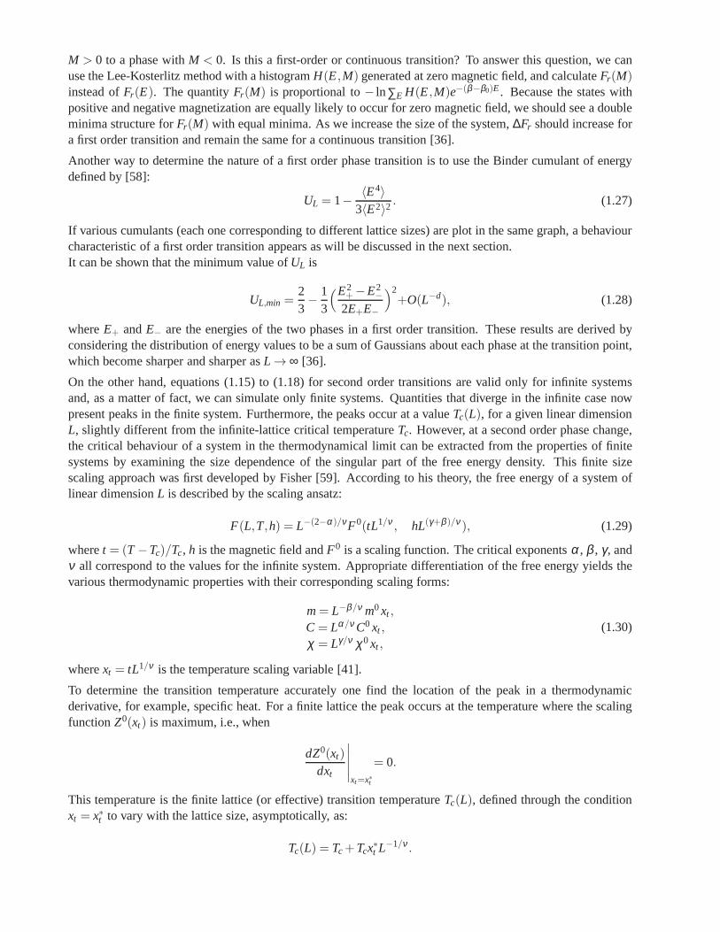
Research of properties of lattices distinct from the commonly studied ones (square, triangular lattice) is akey step in the development and prediction of the behaviour of possible new materials. A different latticeproposed by Donald Betts is constructed removing 1\7 of the sites in a two dimensional triangular lattice [65],accomplishing that each vertex has a coordination number offive and yielding another translationally invariantlattice (see Fig.1.7). This structure is known as Betts or Maple Leaf lattice, and lies between the kagomé andtriangular ones, which have coordination numbers of four and six, respectively. It has a hexagonal unit cell ofsix sites and fifteen bonds, it is invariant under rotations through multiples of 60◦, and, contrary to the kagoméand honeycomb lattices, it has no inversion symmetry [66]. To study the critical behaviour of this lattice, we
performed Monte Carlo simulations using the Potts model forq= 3, q= 4 andq= 5.
Figure 1.7: Maple Leaf lattice
For the q-Potts model, the magnetization is defined as follows:
m=Nmax−1/q
1−1/q, (1.33)
whereNmax is the maximum number of equally oriented spins for certain configuration. We denote the linealsize of the system studied asL, and this is related to the number of sites asnsit = L× L× 6. Earlier workhas been already done on this lattice forq= 3, using the Metropolis algorithm, by Wang and Southern [67].We applied Wolff algorithm instead, due to its proved betterperformance, and obtained similar results forferromagnetic and antiferromagnetic cases. As predicted,calculations shown a second order transition for theferromagnetic case and a first order transition for the antiferromagnetic case. Forq= 4 andq= 5 there is nopublished work. We focus on the ferromagnetic regime in which the transition is found to be of second orderfor q= 4 and of first order forq= 5. In the latter case, the transition is very weak and more calculations areneeded to obtain better results.
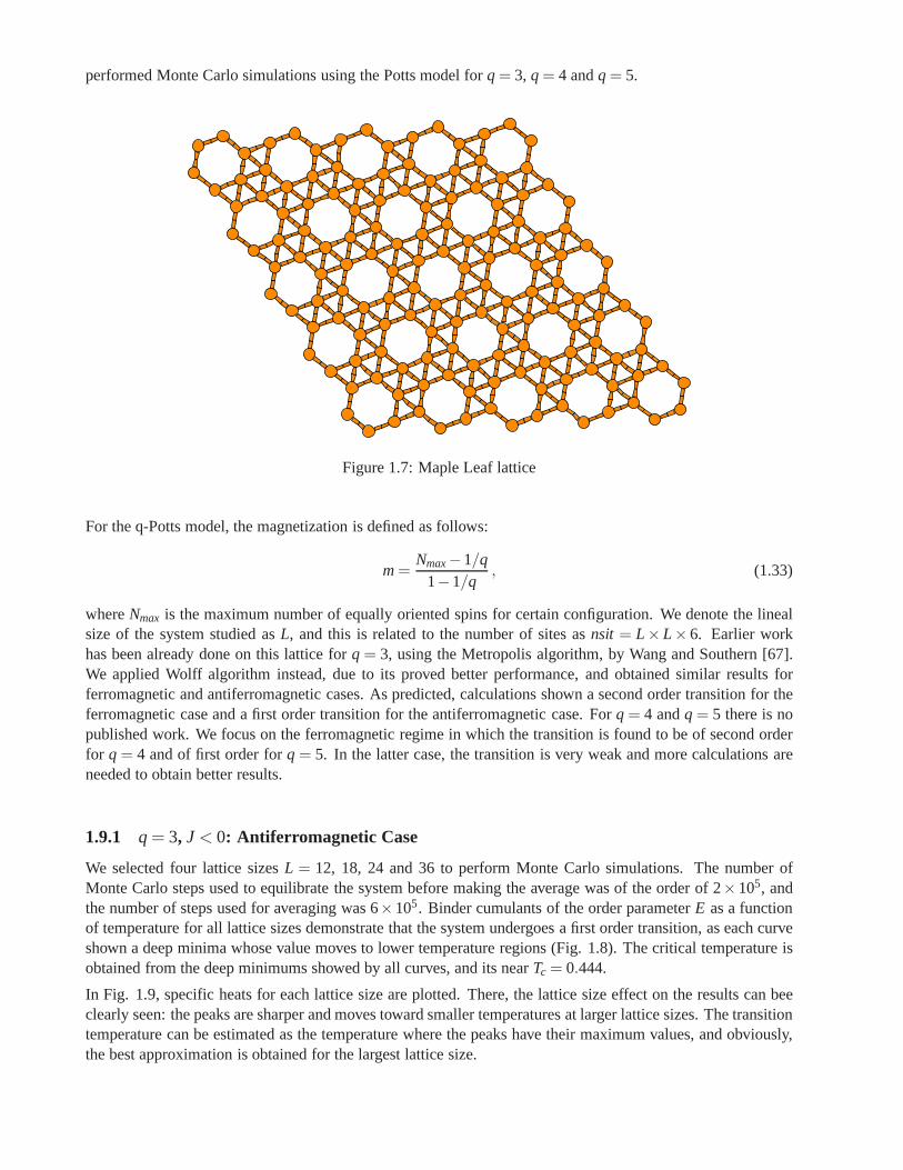
1.9.1 q= 3, J < 0: Antiferromagnetic Case
We selected four lattice sizesL = 12, 18, 24 and 36 to perform Monte Carlo simulations. The number ofMonte Carlo steps used to equilibrate the system before making the average was of the order of 2×10⁵, andthe number of steps used for averaging was 6×10⁵. Binder cumulants of the order parameterE as a functionof temperature for all lattice sizes demonstrate that the system undergoes a first order transition, as each curveshown a deep minima whose value moves to lower temperature regions (Fig. 1.8). The critical temperature isobtained from the deep minimums showed by all curves, and itsnearTc = 0.444.
In Fig. 1.9, specific heats for each lattice size are plotted. There, the lattice size effect on the results can beeclearly seen: the peaks are sharper and moves toward smallertemperatures at larger lattice sizes. The transitiontemperature can be estimated as the temperature where the peaks have their maximum values, and obviously,the best approximation is obtained for the largest lattice size.
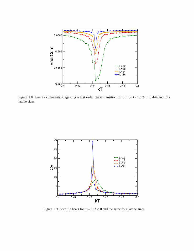
0.4 0.42 0.44 0.46 0.48 0.5
kT0.665
0.6655
0.666
0.6665
Ene
rCum
L=12L=18L=24L=36
Figure 1.8: Energy cumulants suggesting a first order phase transition forq= 3, J < 0, Tc = 0.444 and fourlattice sizes.
0.4 0.42 0.44 0.46 0.48 0.5
kT
5
10
15
20
25
30
Cv
L=12L=18L=24L=36
Figure 1.9: Specific heats forq= 3, J < 0 and the same four lattice sizes.
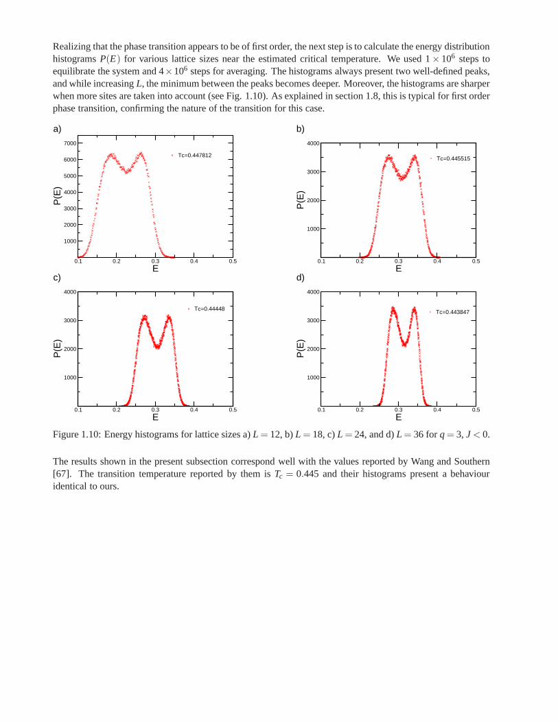
Realizing that the phase transition appears to be of first order, the next step is to calculate the energy distributionhistogramsP(E) for various lattice sizes near the estimated critical temperature. We used 1× 10⁶ steps toequilibrate the system and 4×10⁶ steps for averaging. The histograms always present two well-defined peaks,and while increasingL, the minimum between the peaks becomes deeper. Moreover, the histograms are sharperwhen more sites are taken into account (see Fig. 1.10). As explained in section 1.8, this is typical for first orderphase transition, confirming the nature of the transition for this case.
0.1 0.2 0.3 0.4 0.5
E
1000
2000
3000
4000
5000
6000
7000
P(E
)
Tc=0.447812
a)
0.1 0.2 0.3 0.4 0.5
E
1000
2000
3000
4000
P(E
)
Tc=0.445515
b)
0.1 0.2 0.3 0.4 0.5
E
1000
2000
3000
4000
P(E
)
Tc=0.44448
c)
0.1 0.2 0.3 0.4 0.5
E
1000
2000
3000
4000
P(E
)Tc=0.443847
d)
Figure 1.10: Energy histograms for lattice sizes a)L = 12, b)L = 18, c)L = 24, and d)L= 36 forq= 3, J< 0.
The results shown in the present subsection correspond wellwith the values reported by Wang and Southern[67]. The transition temperature reported by them isTc = 0.445 and their histograms present a behaviouridentical to ours.
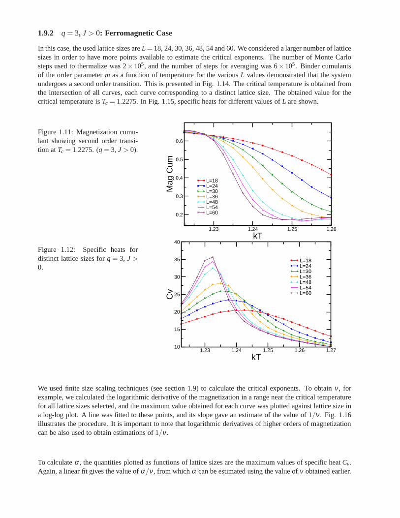
1.9.2 q= 3, J > 0: Ferromagnetic Case
In this case, the used lattice sizes areL= 18, 24, 30, 36, 48, 54 and 60. We considered a larger number of latticesizes in order to have more points available to estimate the critical exponents. The number of Monte Carlosteps used to thermalize was 2×10⁵, and the number of steps for averaging was 6×10⁵. Binder cumulantsof the order parameterm as a function of temperature for the variousL values demonstrated that the systemundergoes a second order transition. This is presented in Fig. 1.14. The critical temperature is obtained fromthe intersection of all curves, each curve corresponding toa distinct lattice size. The obtained value for thecritical temperature isTc = 1.2275. In Fig. 1.15, specific heats for different values ofL are shown.
Figure 1.11: Magnetization cumu-lant showing second order transi-tion atTc = 1.2275. (q= 3, J > 0).
1.23 1.24 1.25 1.26
kT
0.2
0.3
0.4
0.5
0.6
Mag
Cum
L=18L=24L=30L=36L=48L=54L=60
Figure 1.12: Specific heats fordistinct lattice sizes forq= 3, J >0.
1.23 1.24 1.25 1.26 1.27
kT10
15
20
25
30
35
40
Cv
L=18L=24L=30L=36L=48L=54L=60
We used finite size scaling techniques (see section 1.9) to calculate the critical exponents. To obtainν , forexample, we calculated the logarithmic derivative of the magnetization in a range near the critical temperaturefor all lattice sizes selected, and the maximum value obtained for each curve was plotted against lattice size ina log-log plot. A line was fitted to these points, and its slopegave an estimate of the value of 1/ν . Fig. 1.16illustrates the procedure. It is important to note that logarithmic derivatives of higher orders of magnetizationcan be also used to obtain estimations of 1/ν .
To calculateα , the quantities plotted as functions of lattice sizes are the maximum values of specific heatCv.Again, a linear fit gives the value ofα/ν , from whichα can be estimated using the value ofν obtained earlier.
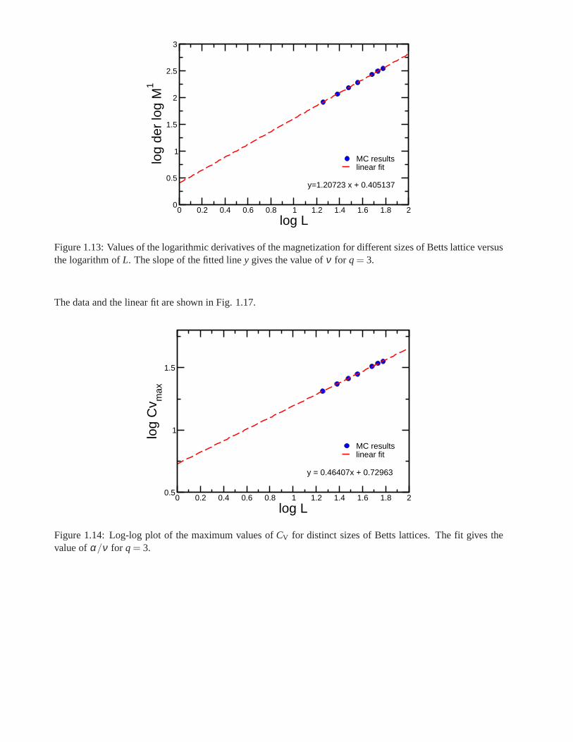
0 0.2 0.4 0.6 0.8 1 1.2 1.4 1.6 1.8 2
log L0
0.5
1
1.5
2
2.5
3
log
der
log
M1
MC results linear fit
y=1.20723 x + 0.405137
Figure 1.13: Values of the logarithmic derivatives of the magnetization for different sizes of Betts lattice versusthe logarithm ofL. The slope of the fitted liney gives the value ofν for q= 3.
The data and the linear fit are shown in Fig. 1.17.
0 0.2 0.4 0.6 0.8 1 1.2 1.4 1.6 1.8 2
log L0.5
1
1.5
log
Cv m
ax
MC resultslinear fit
y = 0.46407x + 0.72963
Figure 1.14: Log-log plot of the maximum values ofCV for distinct sizes of Betts lattices. The fit gives thevalue ofα/ν for q= 3.
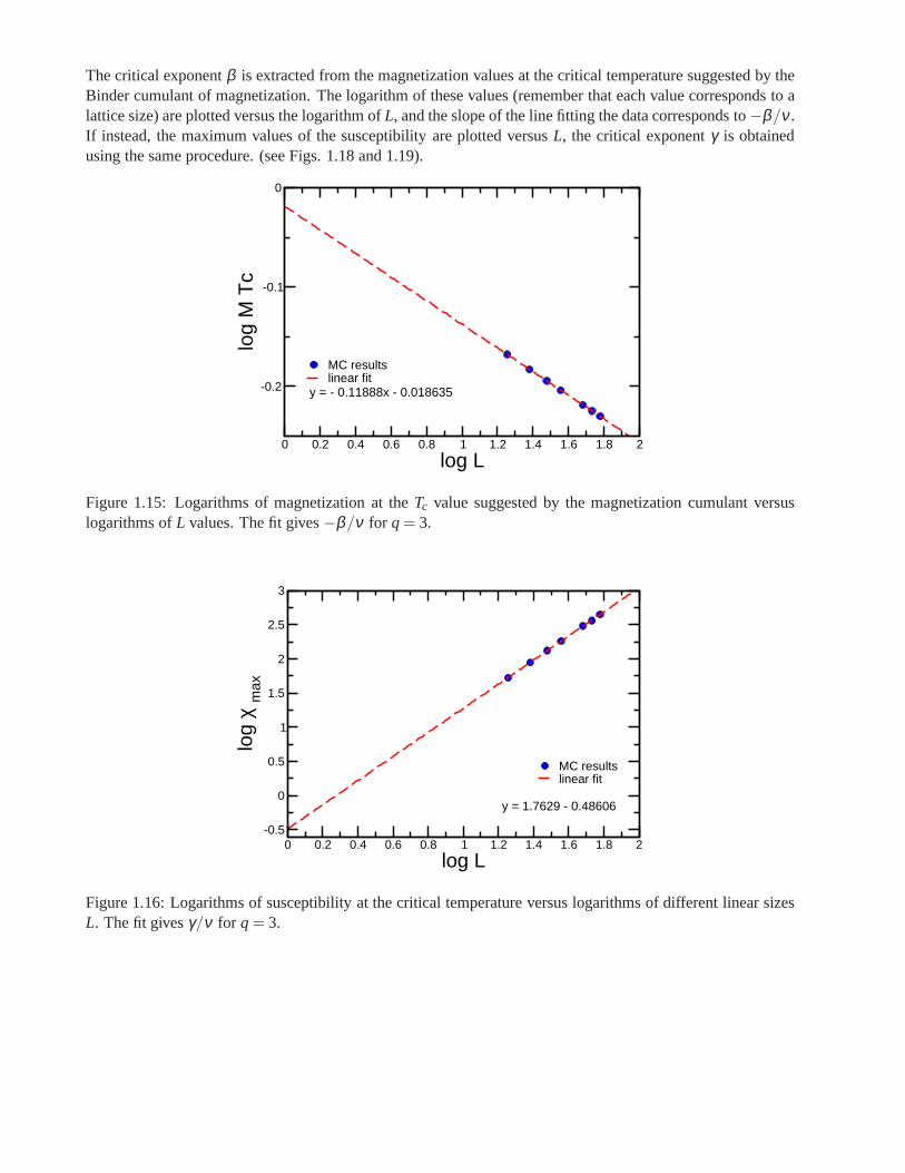
The critical exponentβ is extracted from the magnetization values at the critical temperature suggested by theBinder cumulant of magnetization. The logarithm of these values (remember that each value corresponds to alattice size) are plotted versus the logarithm ofL, and the slope of the line fitting the data corresponds to−β/ν .If instead, the maximum values of the susceptibility are plotted versusL, the critical exponentγ is obtainedusing the same procedure. (see Figs. 1.18 and 1.19).
0 0.2 0.4 0.6 0.8 1 1.2 1.4 1.6 1.8 2
log L
-0.2
-0.1
0
log
M T
c
MC resultslinear fit
y = - 0.11888x - 0.018635
Figure 1.15: Logarithms of magnetization at theTc value suggested by the magnetization cumulant versuslogarithms ofL values. The fit gives−β/ν for q= 3.
0 0.2 0.4 0.6 0.8 1 1.2 1.4 1.6 1.8 2
log L
-0.5
0
0.5
1
1.5
2
2.5
3
log
χ m
ax
MC resultslinear fit
y = 1.7629 - 0.48606
Figure 1.16: Logarithms of susceptibility at the critical temperature versus logarithms of different linear sizesL. The fit givesγ/ν for q= 3.
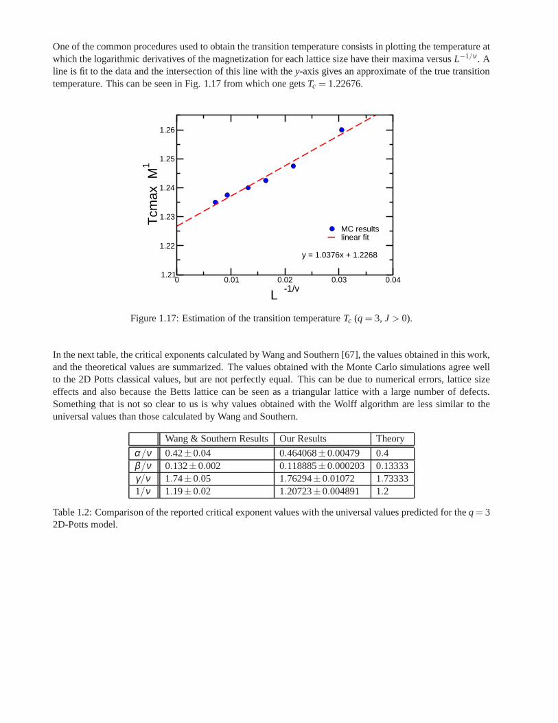
One of the common procedures used to obtain the transition temperature consists in plotting the temperature atwhich the logarithmic derivatives of the magnetization foreach lattice size have their maxima versusL−1/ν . Aline is fit to the data and the intersection of this line with the y-axis gives an approximate of the true transitiontemperature. This can be seen in Fig. 1.17 from which one getsTc = 1.22676.
0 0.01 0.02 0.03 0.04
L -1/v
1.21
1.22
1.23
1.24
1.25
1.26
Tcm
ax M
1
MC resultslinear fit
y = 1.0376x + 1.2268
Figure 1.17: Estimation of the transition temperatureTc (q= 3, J > 0).
In the next table, the critical exponents calculated by Wangand Southern [67], the values obtained in this work,and the theoretical values are summarized. The values obtained with the Monte Carlo simulations agree wellto the 2D Potts classical values, but are not perfectly equal. This can be due to numerical errors, lattice sizeeffects and also because the Betts lattice can be seen as a triangular lattice with a large number of defects.Something that is not so clear to us is why values obtained with the Wolff algorithm are less similar to theuniversal values than those calculated by Wang and Southern.
Wang & Southern Results Our Results Theory
α/ν 0.42±0.04 0.464068±0.00479 0.4β/ν 0.132±0.002 0.118885±0.000203 0.13333γ/ν 1.74±0.05 1.76294±0.01072 1.733331/ν 1.19±0.02 1.20723±0.004891 1.2
Table 1.2: Comparison of the reported critical exponent values with the universal values predicted for theq= 32D-Potts model.
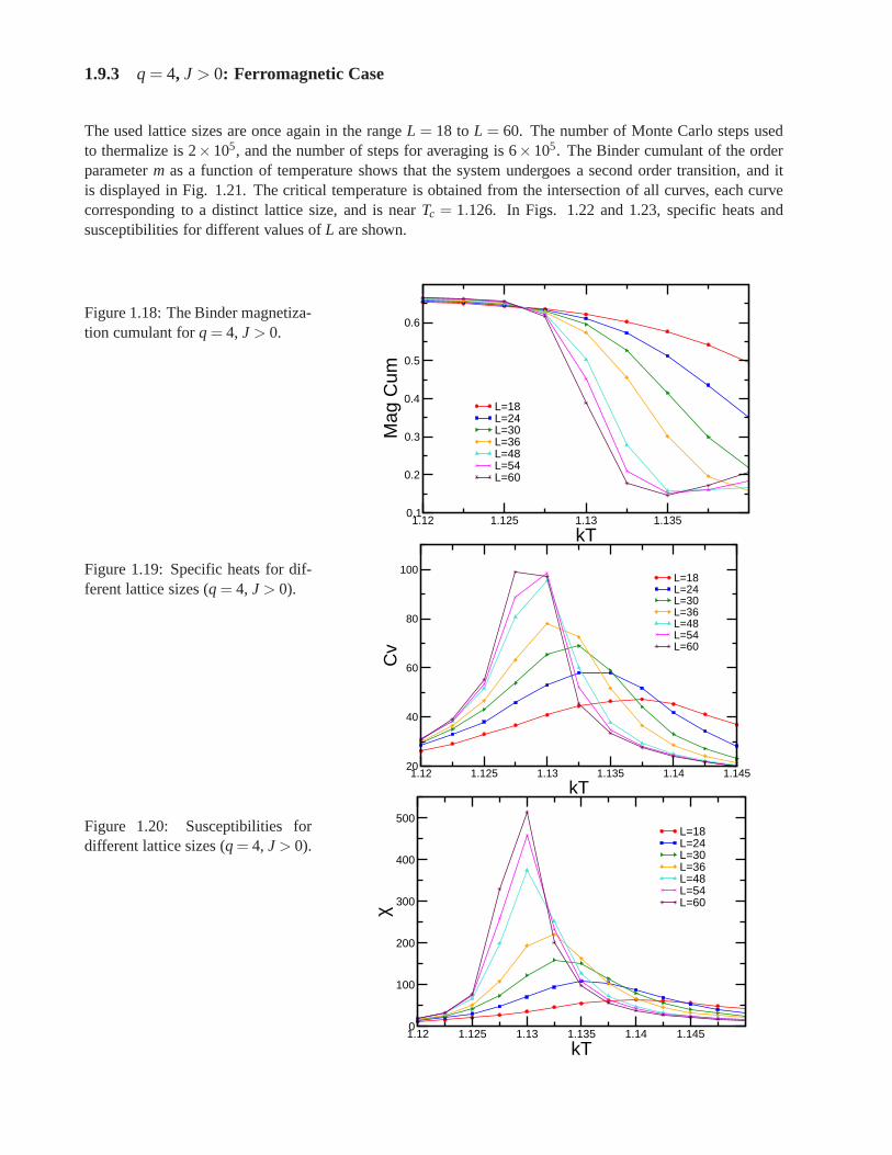
1.9.3 q= 4, J > 0: Ferromagnetic Case
The used lattice sizes are once again in the rangeL = 18 toL = 60. The number of Monte Carlo steps usedto thermalize is 2×10⁵, and the number of steps for averaging is 6×10⁵. The Binder cumulant of the orderparameterm as a function of temperature shows that the system undergoesa second order transition, and itis displayed in Fig. 1.21. The critical temperature is obtained from the intersection of all curves, each curvecorresponding to a distinct lattice size, and is nearTc = 1.126. In Figs. 1.22 and 1.23, specific heats andsusceptibilities for different values ofL are shown.
Figure 1.18: The Binder magnetiza-tion cumulant forq= 4, J > 0.
1.12 1.125 1.13 1.135
kT0.1
0.2
0.3
0.4
0.5
0.6
Mag
Cum
L=18L=24L=30L=36L=48L=54L=60
Figure 1.19: Specific heats for dif-ferent lattice sizes (q= 4, J > 0).
1.12 1.125 1.13 1.135 1.14 1.145
kT20
40
60
80
100
Cv
L=18L=24L=30L=36L=48L=54L=60
Figure 1.20: Susceptibilities fordifferent lattice sizes (q= 4, J> 0).
1.12 1.125 1.13 1.135 1.14 1.145
kT0
100
200
300
400
500
χ
L=18L=24L=30L=36L=48L=54L=60
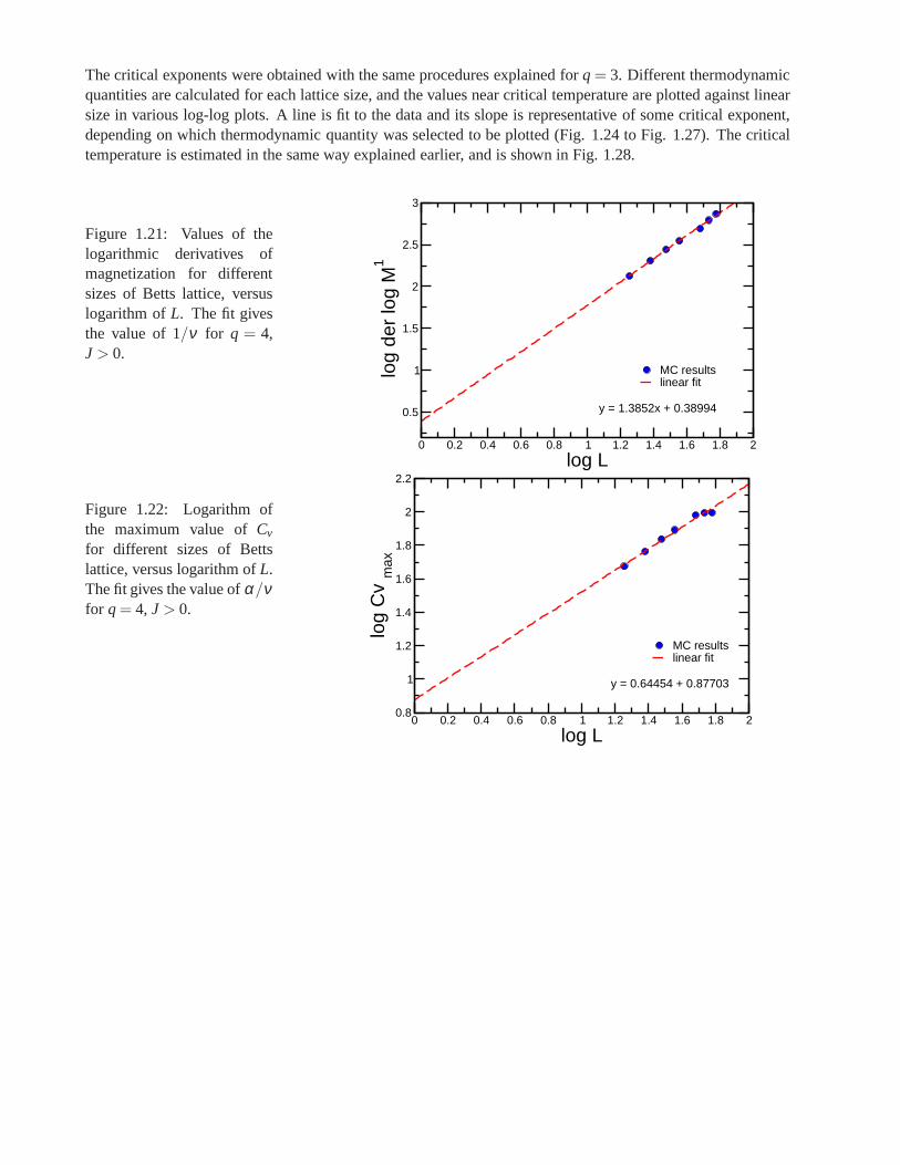
The critical exponents were obtained with the same procedures explained forq= 3. Different thermodynamicquantities are calculated for each lattice size, and the values near critical temperature are plotted against linearsize in various log-log plots. A line is fit to the data and its slope is representative of some critical exponent,depending on which thermodynamic quantity was selected to be plotted (Fig. 1.24 to Fig. 1.27). The criticaltemperature is estimated in the same way explained earlier,and is shown in Fig. 1.28.
Figure 1.21: Values of thelogarithmic derivatives ofmagnetization for differentsizes of Betts lattice, versuslogarithm ofL. The fit givesthe value of 1/ν for q = 4,J > 0.
0 0.2 0.4 0.6 0.8 1 1.2 1.4 1.6 1.8 2
log L
0.5
1
1.5
2
2.5
3
log
der
log
M1
MC resultslinear fit
y = 1.3852x + 0.38994
Figure 1.22: Logarithm ofthe maximum value ofCv
for different sizes of Bettslattice, versus logarithm ofL.The fit gives the value ofα/νfor q= 4, J > 0.
0 0.2 0.4 0.6 0.8 1 1.2 1.4 1.6 1.8 2
log L0.8
1
1.2
1.4
1.6
1.8
2
2.2
log
Cv
max
MC resultslinear fit
y = 0.64454 + 0.87703
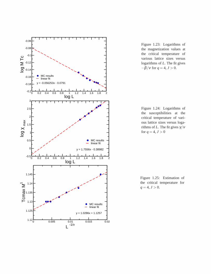
0 0.2 0.4 0.6 0.8 1 1.2 1.4 1.6 1.8 2
log L-0.2
-0.18
-0.16
-0.14
-0.12
-0.1
-0.08
-0.06
log
M T
c
MC resultslinear fit
y = -0.056253x - 0.0791
Figure 1.23: Logarithms ofthe magnetization values atthe critical temperature ofvarious lattice sizes versuslogarithms ofL. The fit gives−β/ν for q= 4, J > 0.
0 0.2 0.4 0.6 0.8 1 1.2 1.4 1.6 1.8 2
log L-0.5
0
0.5
1
1.5
2
2.5
3
log
χ m
ax
MC resultslinear fit
y = 1.7556x - 0.38982
Figure 1.24: Logarithms ofthe susceptibilities at thecritical temperature of vari-ous lattice sizes versus loga-rithms ofL. The fit givesγ/νfor q= 4, J > 0
0 0.005 0.01 0.015 0.02
L -1/v
1.12
1.125
1.13
1.135
1.14
1.145
Tcm
ax M
1
MC resultslinear fit
y = 1.0286x + 1.1257
Figure 1.25: Estimation ofthe critical temperature forq= 4, J > 0.
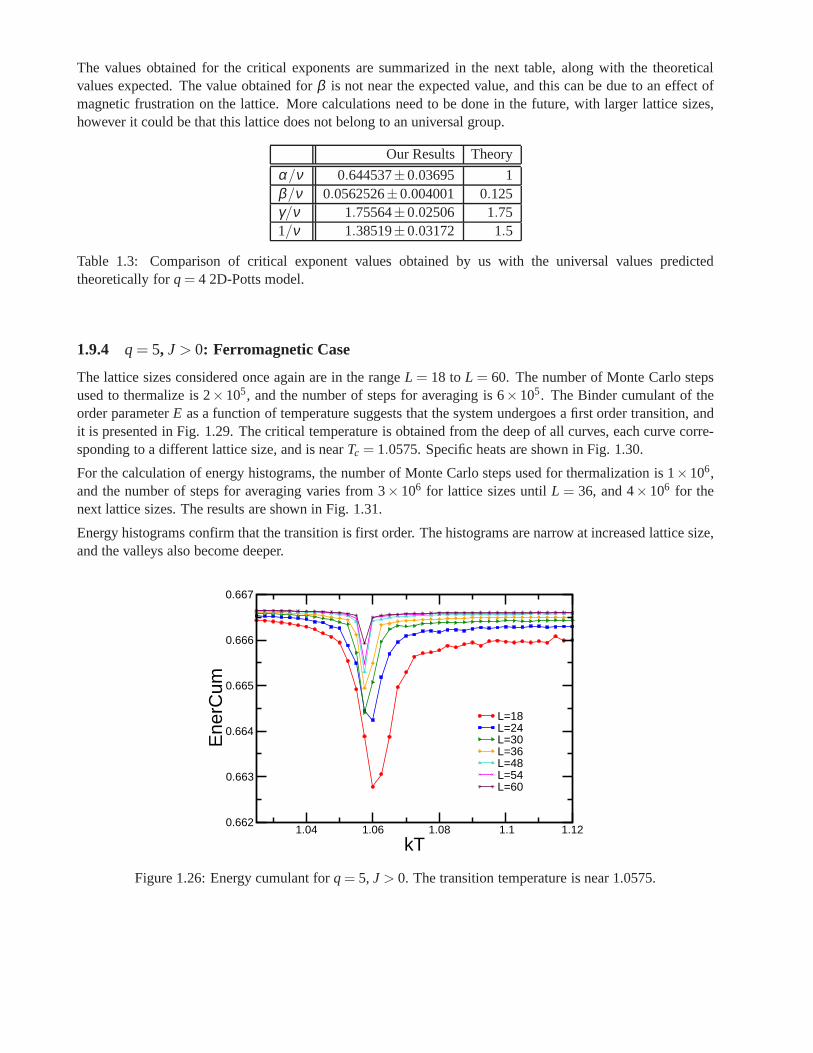
The values obtained for the critical exponents are summarized in the next table, along with the theoreticalvalues expected. The value obtained forβ is not near the expected value, and this can be due to an effectofmagnetic frustration on the lattice. More calculations need to be done in the future, with larger lattice sizes,however it could be that this lattice does not belong to an universal group.
Our Results Theory
α/ν 0.644537±0.03695 1β/ν 0.0562526±0.004001 0.125γ/ν 1.75564±0.02506 1.751/ν 1.38519±0.03172 1.5
Table 1.3: Comparison of critical exponent values obtainedby us with the universal values predictedtheoretically forq= 4 2D-Potts model.
1.9.4 q= 5, J > 0: Ferromagnetic Case
The lattice sizes considered once again are in the rangeL = 18 toL = 60. The number of Monte Carlo stepsused to thermalize is 2×10⁵, and the number of steps for averaging is 6×10⁵. The Binder cumulant of theorder parameterE as a function of temperature suggests that the system undergoes a first order transition, andit is presented in Fig. 1.29. The critical temperature is obtained from the deep of all curves, each curve corre-sponding to a different lattice size, and is nearTc = 1.0575. Specific heats are shown in Fig. 1.30.
For the calculation of energy histograms, the number of Monte Carlo steps used for thermalization is 1×10⁶,and the number of steps for averaging varies from 3× 10⁶ for lattice sizes untilL = 36, and 4× 10⁶ for thenext lattice sizes. The results are shown in Fig. 1.31.
Energy histograms confirm that the transition is first order. The histograms are narrow at increased lattice size,and the valleys also become deeper.
1.04 1.06 1.08 1.1 1.12
kT0.662
0.663
0.664
0.665
0.666
0.667
Ene
rCum
L=18L=24L=30L=36L=48L=54L=60
Figure 1.26: Energy cumulant forq= 5, J > 0. The transition temperature is near 1.0575.
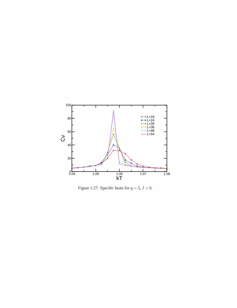
1.04 1.05 1.06 1.07 1.08
kT0
20
40
60
80
100
Cv
L=18L=24L=30L=36L=48L=54
Figure 1.27: Specific heats forq= 5, J > 0.
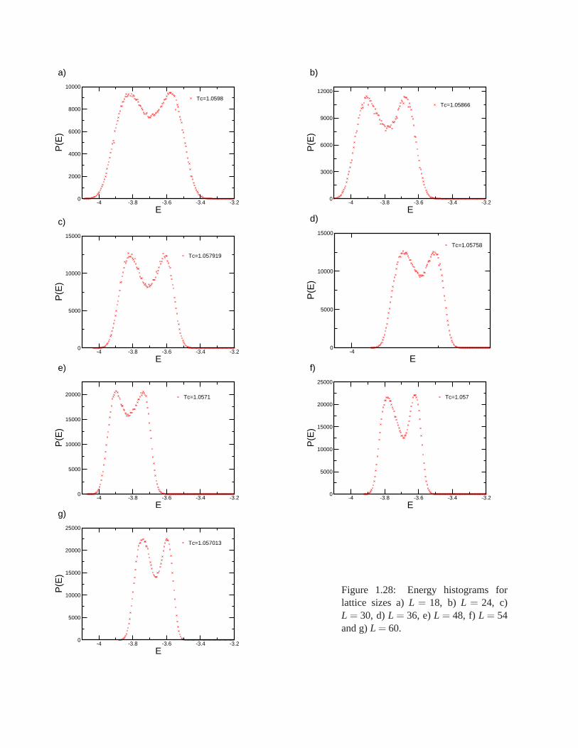
-4 -3.8 -3.6 -3.4 -3.2
E0
2000
4000
6000
8000
10000
P(E
)
Tc=1.0598
a)
-4 -3.8 -3.6 -3.4 -3.2
E0
3000
6000
9000
12000
P(E
)
Tc=1.05866
b)
-4 -3.8 -3.6 -3.4 -3.2
E0
5000
10000
15000
P(E
)
Tc=1.057919
c)
-4
E0
5000
10000
15000
P(E
)
Tc=1.05758
d)
-4 -3.8 -3.6 -3.4 -3.2
E0
5000
10000
15000
20000
P(E
)
Tc=1.0571
e)
-4 -3.8 -3.6 -3.4 -3.2
E0
5000
10000
15000
20000
25000
P(E
)
Tc=1.057
f)
-4 -3.8 -3.6 -3.4 -3.2
E0
5000
10000
15000
20000
25000
P(E
)
Tc=1.057013
g)
Figure 1.28: Energy histograms forlattice sizes a)L = 18, b) L = 24, c)L = 30, d)L = 36, e)L = 48, f) L = 54and g)L = 60.

1.9.5 Conclusion
The results obtained with Monte Carlo simulations and finitesize scaling techniques show clearly the kind oftransition for each of the cases presented. The calculated critical exponents were near the theoretical valuesfor second order phase transitions, except for the exponentβ in the caseq= 4 that requires a more detailedanalysis. Remember that forJ > 0 the transition is supposed to be of second order forq≤ 4 and of first orderfor q> 4. As it lies at the border between the two, the caseq = 4 is difficult to assess. Another aspect thatmust be taken into account for further analysis is the type oflattice, because it is quite probable that magneticfrustration effects could modify the magnetization-related critical coefficients. For first order transitions, thevalues of the free energy barriers could be estimated from the difference between the two peaks and the valley.
As we mentioned at the end of section 1.1, Monte Carlo simulations are a helpful tool in other areas. Thus,in the next chapter we will move on and review a cluster identification technique that involves Monte Carlocalculations for the analysis of biological data.

Chapter 2
Monte Carlo Simulations in Biology
Contents
2.1 Proteins, DNA and Gene Expression . . . . . . . . . . . . . . . . . . .. . . . . . . . . . 37
2.2 DNA Microarrays . . . . . . . . . . . . . . . . . . . . . . . . . . . . . . . . . .. . . . . 38
2.3 Gene Clustering . . . . . . . . . . . . . . . . . . . . . . . . . . . . . . . . . .. . . . . . 39
2.3.1 Hierarchical Clustering . . . . . . . . . . . . . . . . . . . . . . . .. . . . . . . . . 41
2.3.2 K-Means Clustering . . . . . . . . . . . . . . . . . . . . . . . . . . . . .. . . . . 42
2.3.3 Self-Organizing Maps . . . . . . . . . . . . . . . . . . . . . . . . . . .. . . . . . 42
2.3.4 Self-Organizing Tree Algorithm . . . . . . . . . . . . . . . . . .. . . . . . . . . . 42
2.3.5 Model Based Clustering . . . . . . . . . . . . . . . . . . . . . . . . . .. . . . . . 43
2.3.6 Quality-Based Algorithms . . . . . . . . . . . . . . . . . . . . . . .. . . . . . . . 44
2.3.7 Adaptive Quality-Based Clustering . . . . . . . . . . . . . . .. . . . . . . . . . . 45
2.3.8 Biclustering and Some Physics Related Algorithms . . .. . . . . . . . . . . . . . . 45
2.4 Superparamagnetic Gene Clustering: Monte Carlo Simulations . . . . . . . . . . . . . 46
2.4.1 Detailed Description of SPC . . . . . . . . . . . . . . . . . . . . . .. . . . . . . . 47
2.4.2 Future Directions . . . . . . . . . . . . . . . . . . . . . . . . . . . . . .. . . . . . 48
36
2.1 Proteins, DNA and Gene Expression
Proteins are the complex molecules that make life possible.Keratin, essential in the structural conformationof our hair and nails, is one among the many proteins used as supporting materials in biology. Cells are alsomade of proteins, and enzymes, which are responsible for allchemical reactions inside living organisms, areproteins too. The information to produce the sequence of amino acids conforming certain protein resides inthe DNA molecule, making it of great importance for life.
A single strand of DNA is formed by unities named nucleotides. Each nucleotide is composed by deoxyribose(a sugar formed by five carbons), a phosphate group, and one ofthe four possible nitrogenous bases: adenine(A), cytosine (C), guanine (G) and thymine (G). Phosphodiester bridges link the phosphate group of anucleotide and the sugar of the next one, building in this waya chain of nucleotides. The DNA moleculeis formed when two of these linear chains are joined by hydrogen bonds connecting the nitrogenous basesstanding out of the sugar-phosphate backbone of each chain.All this chemical construction has a double helixstructure envisioned in 1952 by Cricks and Watson [1]. The diameter of the helix is of 2 nm, and adjacentbases are separated by 0.34 nm along the helix axis. Hence, the helix repeats itself every 10 residues on eachchain at intervals of 3.4 nm. Only specific pairs of bases can form hydrogen bonds: the purine base A alwayspairs with the pyrimidine base T through two hydrogen bonds,and the other pyrimidine base C always pairswith the purine base G this time by three hydrogen bonds [2]. Apossible explanation for this situation is thattwo purines require more than 2 nm for connection, which doesnot fit within the diameter of the helix. On theother hand, there is too much space for two pyrimidines to getclose enough to form hydrogen bonds betweenthem [3]. The rules of base pairing tell us that if we can “read” the sequence of nucleotides on one strandof DNA, we can immediately infer the complementary sequenceon the other strand. Thus, DNA looks likea chemical code based on four letters, each one corresponding to the four nitrogenous bases, aligned along adouble-helicoidal chain. At the same time, the genetic codeis a universal translation table formed by three-bases words called codons. Each codon codifies for a specific amino acid, so different sequences of codonsbuild distinct proteins, and they can also build RNA molecules with a functional role. One can obtain 64distinct combinations mixing the four nitrogenous bases inclusters of three letters. This quantity is enough tocode for the 20 amino acids forming all proteins, and, as a matter of fact, almost all amino acids have morethan one codon to codify them. Three of these triplets are left apart to code for chain termination to releaseproteins at the end of their production process. Moreover, one triplet is left as a signal to start the synthesisprocess. A segment of DNA sequence with the instructions to codify for a functional product, protein or RNA,is named a gene, and the genome is the collection of all the “recipes” for the products that an organism needs.The genome of a simple organism such as yeast has around 7,000genes and the latest estimate for the humangenome is of 25,000 genes [4]. It is important to stress that not all chain segments codify for proteins or RNAmolecules: an overwhelming majority of human DNA (98%) contains non-coding regions (introns) that do notrepresent any particular functional product [5], althoughit is believed that they help to protect the genes.
Every cell of multicellular organisms has the entire set of information needed, but only some genes areexpressed depending on the function of the cell. For example, cells in our retina need photosensitive molecules,whereas our liver do not.A gene is expressed in a cell when the protein or RNA it codes for is synthesized.The large majority of abundantly expressed genes are associated with common functions, such as metabolism,and hence are expressed in all cells. However, there will be differences in the expression profiles of differentcells, and even in a single cell, expression will vary with time, in a manner dictated by external and internalsignals that reflect the state of the organism and the cell itself [5].
Although DNA molecule contains all the instructions to makea huge amount of diverse proteins, DNA is notable to come out of the eucaryotic cell nucleus. Therefore, when certain protein is needed, another moleculecalled messenger RNA (m-RNA) is formed from DNA in a fundamental process called transcription, and isthis molecule who travels outside the nucleus carrying the information. RNA is also a nucleic acid but isformed by a single of nucleotides, and its sugar (ribose) is slightly different from deoxyribose. Besides, RNAhas uracil U instead of the base thymine T. In cells, one can find three important types of RNA: messenger
RNA (m-RNA), which transports the instructions to make a protein from the nucleus to the ribosomes, transferRNA (t-RNA) which carries the amino acids to the ribosomes where the proteins are assembled and is foundin the cytoplasm, and, finally, the r-RNA, or ribosomal RNA, which is one of the substances from what theribosomes are made out [6].
In the transcription process, the portion of DNA containingthe sequence for the needed product splits off, andthen the free RNA nucleotides existing in the nucleus are attached to the exposed DNA nucleotides forminga complementary chain of RNA. This m-RNA chain comes out of the nucleus carrying a complementarysequence and arrives finally to the ribosome, where the sequence is translated into a protein(translationprocess). A cell may need a large number of some proteins and asmall number of others, i.e. every genemay be expressed at a different level. The manner in which theinstructions to start and stop transcription aregiven for a certain gene is governed by regulatory networks.Transcription is regulated by special proteins,called transcription factors, which bind to specific locations on the DNA, upstream from the coding region.Their presence at the right site initiates or suppresses transcription. The basic paradigm of gene expressionanalysis states that the biological state of a cell is reflected by its expression profile: the expression levels ofall the genes of the genome. These in turn are reflected by the concentrations of the corresponding m-RNAmolecules [5].
Several genomes of diverse organisms have been completed inthe last years, the human genome, published on2002, among them. Now, the main focus is to understand the underlying function and mechanisms behind thesegenomes. Some of the questions that remain unanswered included what are the functional roles of differentgenes, how genes are regulated, how do genes and gene products interact, how does gene expression leveldiffer in various cell types and states, and how is gene expression changed by various diseases or compoundtreatments[7].
2.2 DNA Microarrays
Although m-RNA is not the ultimate product of a gene, transcription is the first step in gene regulation,and information about the transcript levels is needed as a first approach for understanding gene regulatorynetworks. DNA microarrays or DNA chips are one of the latest breakthroughs in experimental molecularbiology precisely because they allow to monitor the expression of thousands of genes at the same time.The potential this technology is tremendous: monitoring gene expression levels in different developmentalstages, tissue types, clinical conditions and different organisms can help understanding gene function and genenetworks, assist in the diagnosis of disease conditions andreveal effects of medical treatments.
There are currently two main technologies that generate large-scale gene expression data: cDNA andoligonucleotide microarrays. CDNA microarrays contain large sets of complementary DNA sequences severalhundred bases long, each set representing a gene, immobilized on a solid substrate. In oligonucleotidemicroarrays, each gene is represented on the array by a set of15-20 different oligonucleotide probes designedto hybridize perfectly to some particular sequence, and some mismatch control oligonucleotides, identical tothe perfect match probes except for a single base-pair mismatch. These mismatch control oligonucleotidesallow estimation of cross-hybridization, improving reproducibility and accuracy of RNA quantification, andreducing the rate of false-positives. In general, oligonucleotides used consist about 20-25 nucleotides, and aresynthesized in situ with photolithography techniques [8],[9]. In brief, functioning of microarrays is based onthe preferential binding of complementary single strandednucleic acid sequences, and a single microarray maycontain tens of thousands of spots. One of the most popular experiments involving cDNA microarrays consistsin compare m-RNA abundance in two samples. The m-RNA molecules are extracted from cells taken from twotissues of interest (e.g. tumour and normal tissues) [10]. They are reverse transcribed from RNA to DNA andtheir concentration is enhanced. The resulting DNA is transcribed back into fluorescently marked single strandRNA. For example, tumour tissue is labeled with a red dye and normal tissue with a green one. The solutionof marked and enhanced m-RNA molecules (“targets”) that arecopies of the m-RNA molecules originallyextracted from the tissue, is placed on the chip and diffusesover the collection of single strand DNA probes.
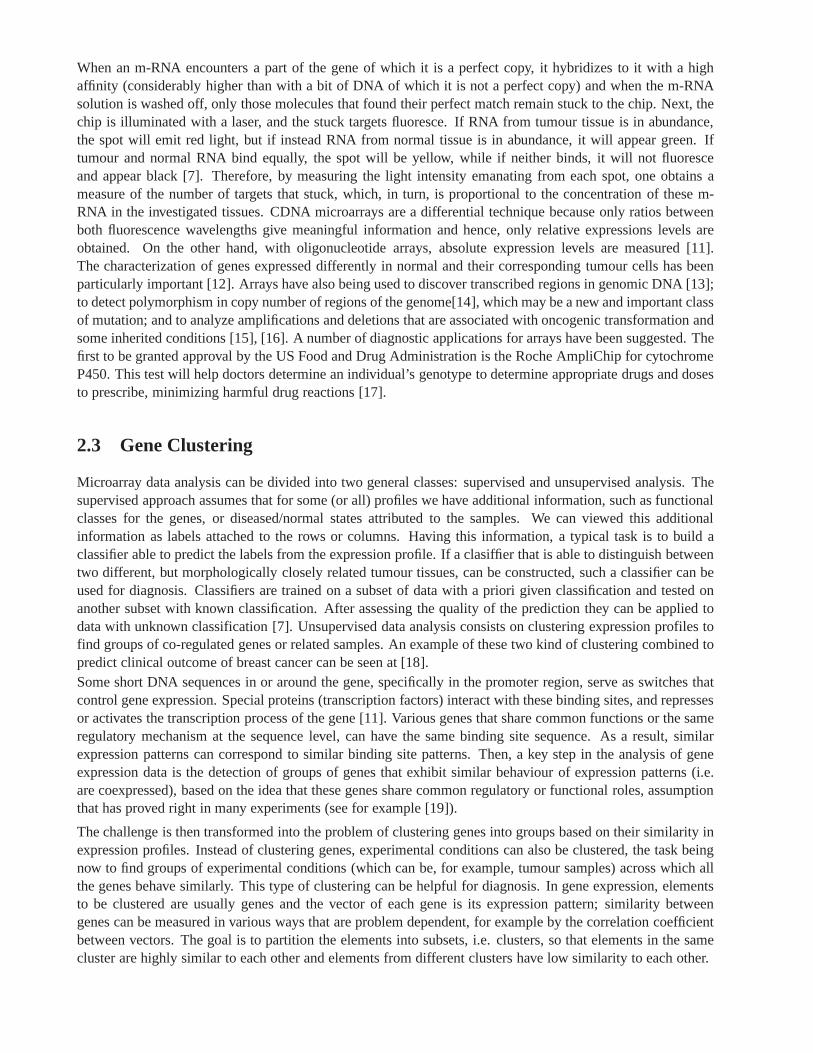
When an m-RNA encounters a part of the gene of which it is a perfect copy, it hybridizes to it with a highaffinity (considerably higher than with a bit of DNA of which it is not a perfect copy) and when the m-RNAsolution is washed off, only those molecules that found their perfect match remain stuck to the chip. Next, thechip is illuminated with a laser, and the stuck targets fluoresce. If RNA from tumour tissue is in abundance,the spot will emit red light, but if instead RNA from normal tissue is in abundance, it will appear green. Iftumour and normal RNA bind equally, the spot will be yellow, while if neither binds, it will not fluoresceand appear black [7]. Therefore, by measuring the light intensity emanating from each spot, one obtains ameasure of the number of targets that stuck, which, in turn, is proportional to the concentration of these m-RNA in the investigated tissues. CDNA microarrays are a differential technique because only ratios betweenboth fluorescence wavelengths give meaningful informationand hence, only relative expressions levels areobtained. On the other hand, with oligonucleotide arrays, absolute expression levels are measured [11].The characterization of genes expressed differently in normal and their corresponding tumour cells has beenparticularly important [12]. Arrays have also being used todiscover transcribed regions in genomic DNA [13];to detect polymorphism in copy number of regions of the genome[14], which may be a new and important classof mutation; and to analyze amplifications and deletions that are associated with oncogenic transformation andsome inherited conditions [15], [16]. A number of diagnostic applications for arrays have been suggested. Thefirst to be granted approval by the US Food and Drug Administration is the Roche AmpliChip for cytochromeP450. This test will help doctors determine an individual’sgenotype to determine appropriate drugs and dosesto prescribe, minimizing harmful drug reactions [17].
2.3 Gene Clustering
Microarray data analysis can be divided into two general classes: supervised and unsupervised analysis. Thesupervised approach assumes that for some (or all) profiles we have additional information, such as functionalclasses for the genes, or diseased/normal states attributed to the samples. We can viewed this additionalinformation as labels attached to the rows or columns. Having this information, a typical task is to build aclassifier able to predict the labels from the expression profile. If a clasiffier that is able to distinguish betweentwo different, but morphologically closely related tumourtissues, can be constructed, such a classifier can beused for diagnosis. Classifiers are trained on a subset of data with a priori given classification and tested onanother subset with known classification. After assessing the quality of the prediction they can be applied todata with unknown classification [7]. Unsupervised data analysis consists on clustering expression profiles tofind groups of co-regulated genes or related samples. An example of these two kind of clustering combined topredict clinical outcome of breast cancer can be seen at [18].Some short DNA sequences in or around the gene, specifically in the promoter region, serve as switches thatcontrol gene expression. Special proteins (transcriptionfactors) interact with these binding sites, and repressesor activates the transcription process of the gene [11]. Various genes that share common functions or the sameregulatory mechanism at the sequence level, can have the same binding site sequence. As a result, similarexpression patterns can correspond to similar binding sitepatterns. Then, a key step in the analysis of geneexpression data is the detection of groups of genes that exhibit similar behaviour of expression patterns (i.e.are coexpressed), based on the idea that these genes share common regulatory or functional roles, assumptionthat has proved right in many experiments (see for example [19]).
The challenge is then transformed into the problem of clustering genes into groups based on their similarity inexpression profiles. Instead of clustering genes, experimental conditions can also be clustered, the task beingnow to find groups of experimental conditions (which can be, for example, tumour samples) across which allthe genes behave similarly. This type of clustering can be helpful for diagnosis. In gene expression, elementsto be clustered are usually genes and the vector of each gene is its expression pattern; similarity betweengenes can be measured in various ways that are problem dependent, for example by the correlation coefficientbetween vectors. The goal is to partition the elements into subsets, i.e. clusters, so that elements in the samecluster are highly similar to each other and elements from different clusters have low similarity to each other.
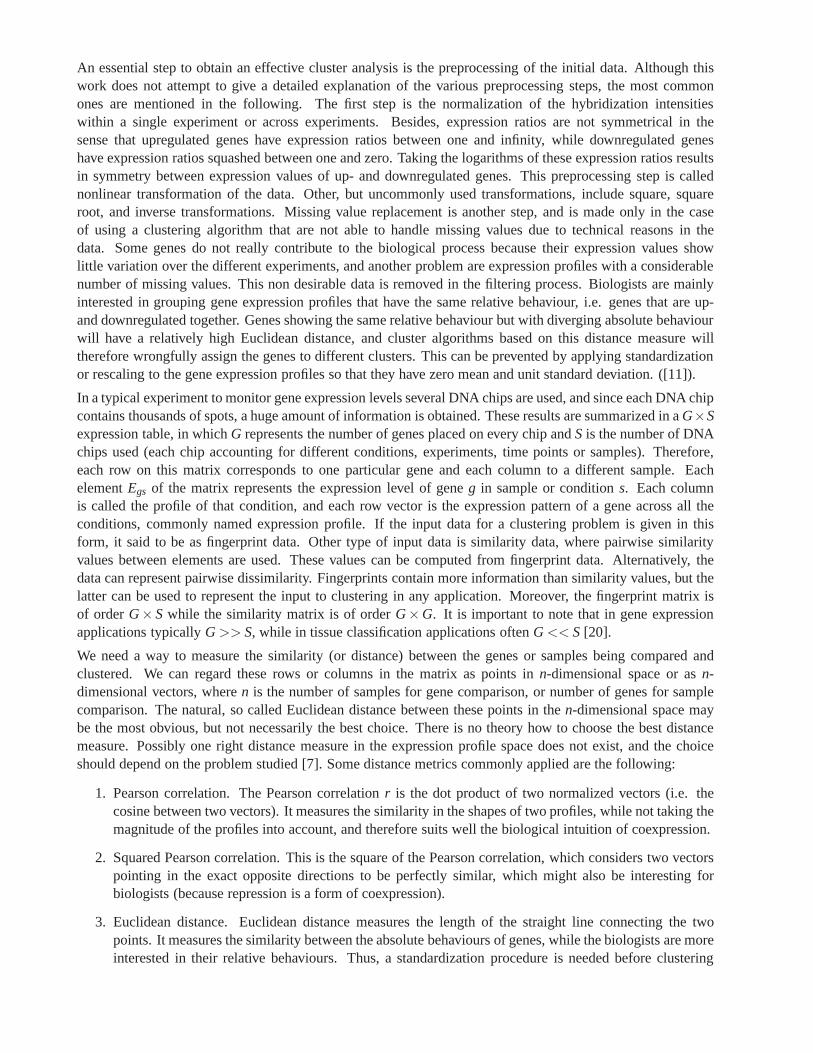
An essential step to obtain an effective cluster analysis isthe preprocessing of the initial data. Although thiswork does not attempt to give a detailed explanation of the various preprocessing steps, the most commonones are mentioned in the following. The first step is the normalization of the hybridization intensitieswithin a single experiment or across experiments. Besides,expression ratios are not symmetrical in thesense that upregulated genes have expression ratios between one and infinity, while downregulated geneshave expression ratios squashed between one and zero. Taking the logarithms of these expression ratios resultsin symmetry between expression values of up- and downregulated genes. This preprocessing step is callednonlinear transformation of the data. Other, but uncommonly used transformations, include square, squareroot, and inverse transformations. Missing value replacement is another step, and is made only in the caseof using a clustering algorithm that are not able to handle missing values due to technical reasons in thedata. Some genes do not really contribute to the biological process because their expression values showlittle variation over the different experiments, and another problem are expression profiles with a considerablenumber of missing values. This non desirable data is removedin the filtering process. Biologists are mainlyinterested in grouping gene expression profiles that have the same relative behaviour, i.e. genes that are up-and downregulated together. Genes showing the same relative behaviour but with diverging absolute behaviourwill have a relatively high Euclidean distance, and clusteralgorithms based on this distance measure willtherefore wrongfully assign the genes to different clusters. This can be prevented by applying standardizationor rescaling to the gene expression profiles so that they havezero mean and unit standard deviation. ([11]).
In a typical experiment to monitor gene expression levels several DNA chips are used, and since each DNA chipcontains thousands of spots, a huge amount of information isobtained. These results are summarized in aG×Sexpression table, in whichG represents the number of genes placed on every chip andS is the number of DNAchips used (each chip accounting for different conditions,experiments, time points or samples). Therefore,each row on this matrix corresponds to one particular gene and each column to a different sample. EachelementEgs of the matrix represents the expression level of geneg in sample or conditions. Each columnis called the profile of that condition, and each row vector isthe expression pattern of a gene across all theconditions, commonly named expression profile. If the inputdata for a clustering problem is given in thisform, it said to be as fingerprint data. Other type of input data is similarity data, where pairwise similarityvalues between elements are used. These values can be computed from fingerprint data. Alternatively, thedata can represent pairwise dissimilarity. Fingerprints contain more information than similarity values, but thelatter can be used to represent the input to clustering in anyapplication. Moreover, the fingerprint matrix isof orderG×S while the similarity matrix is of orderG×G. It is important to note that in gene expressionapplications typicallyG>> S, while in tissue classification applications oftenG<< S [20].
We need a way to measure the similarity (or distance) betweenthe genes or samples being compared andclustered. We can regard these rows or columns in the matrix as points inn-dimensional space or asn-dimensional vectors, wheren is the number of samples for gene comparison, or number of genes for samplecomparison. The natural, so called Euclidean distance between these points in then-dimensional space maybe the most obvious, but not necessarily the best choice. There is no theory how to choose the best distancemeasure. Possibly one right distance measure in the expression profile space does not exist, and the choiceshould depend on the problem studied [7]. Some distance metrics commonly applied are the following:
1. Pearson correlation. The Pearson correlationr is the dot product of two normalized vectors (i.e. thecosine between two vectors). It measures the similarity in the shapes of two profiles, while not taking themagnitude of the profiles into account, and therefore suits well the biological intuition of coexpression.
2. Squared Pearson correlation. This is the square of the Pearson correlation, which considers two vectorspointing in the exact opposite directions to be perfectly similar, which might also be interesting forbiologists (because repression is a form of coexpression).
3. Euclidean distance. Euclidean distance measures the length of the straight line connecting the twopoints. It measures the similarity between the absolute behaviours of genes, while the biologists are moreinterested in their relative behaviours. Thus, a standardization procedure is needed before clustering
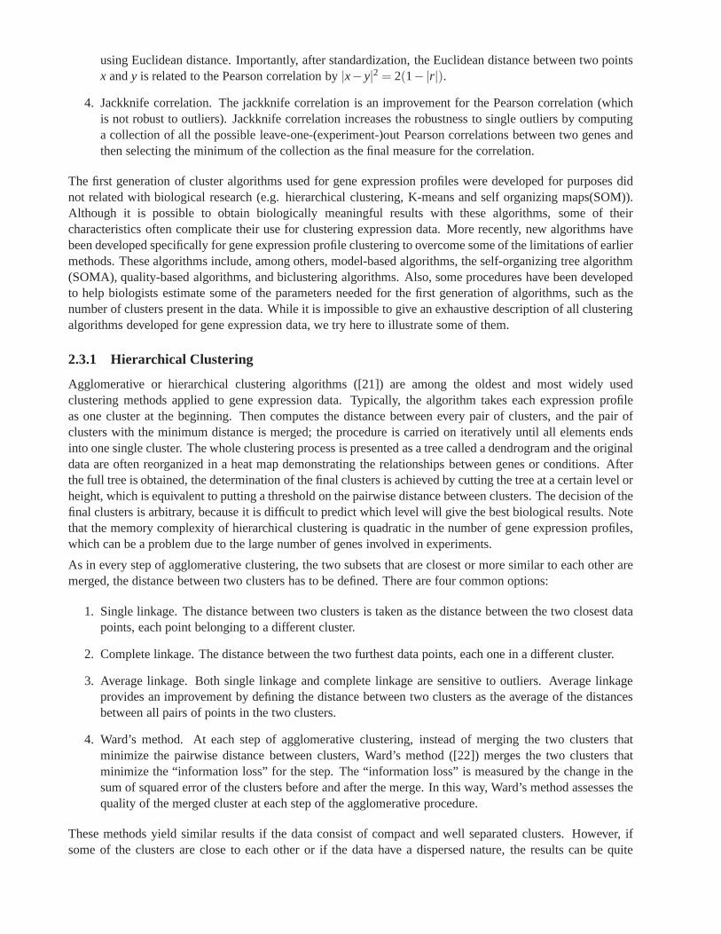
using Euclidean distance. Importantly, after standardization, the Euclidean distance between two pointsx andy is related to the Pearson correlation by|x−y|2 = 2(1−|r|).
4. Jackknife correlation. The jackknife correlation is an improvement for the Pearson correlation (whichis not robust to outliers). Jackknife correlation increases the robustness to single outliers by computinga collection of all the possible leave-one-(experiment-)out Pearson correlations between two genes andthen selecting the minimum of the collection as the final measure for the correlation.
The first generation of cluster algorithms used for gene expression profiles were developed for purposes didnot related with biological research (e.g. hierarchical clustering, K-means and self organizing maps(SOM)).Although it is possible to obtain biologically meaningful results with these algorithms, some of theircharacteristics often complicate their use for clusteringexpression data. More recently, new algorithms havebeen developed specifically for gene expression profile clustering to overcome some of the limitations of earliermethods. These algorithms include, among others, model-based algorithms, the self-organizing tree algorithm(SOMA), quality-based algorithms, and biclustering algorithms. Also, some procedures have been developedto help biologists estimate some of the parameters needed for the first generation of algorithms, such as thenumber of clusters present in the data. While it is impossible to give an exhaustive description of all clusteringalgorithms developed for gene expression data, we try here to illustrate some of them.
2.3.1 Hierarchical Clustering
Agglomerative or hierarchical clustering algorithms ([21]) are among the oldest and most widely usedclustering methods applied to gene expression data. Typically, the algorithm takes each expression profileas one cluster at the beginning. Then computes the distance between every pair of clusters, and the pair ofclusters with the minimum distance is merged; the procedureis carried on iteratively until all elements endsinto one single cluster. The whole clustering process is presented as a tree called a dendrogram and the originaldata are often reorganized in a heat map demonstrating the relationships between genes or conditions. Afterthe full tree is obtained, the determination of the final clusters is achieved by cutting the tree at a certain level orheight, which is equivalent to putting a threshold on the pairwise distance between clusters. The decision of thefinal clusters is arbitrary, because it is difficult to predict which level will give the best biological results. Notethat the memory complexity of hierarchical clustering is quadratic in the number of gene expression profiles,which can be a problem due to the large number of genes involved in experiments.
As in every step of agglomerative clustering, the two subsets that are closest or more similar to each other aremerged, the distance between two clusters has to be defined. There are four common options:
1. Single linkage. The distance between two clusters is taken as the distance between the two closest datapoints, each point belonging to a different cluster.
2. Complete linkage. The distance between the two furthest data points, each one in a different cluster.
3. Average linkage. Both single linkage and complete linkage are sensitive to outliers. Average linkageprovides an improvement by defining the distance between twoclusters as the average of the distancesbetween all pairs of points in the two clusters.
4. Ward’s method. At each step of agglomerative clustering,instead of merging the two clusters thatminimize the pairwise distance between clusters, Ward’s method ([22]) merges the two clusters thatminimize the “information loss” for the step. The “information loss” is measured by the change in thesum of squared error of the clusters before and after the merge. In this way, Ward’s method assesses thequality of the merged cluster at each step of the agglomerative procedure.
These methods yield similar results if the data consist of compact and well separated clusters. However, ifsome of the clusters are close to each other or if the data havea dispersed nature, the results can be quite
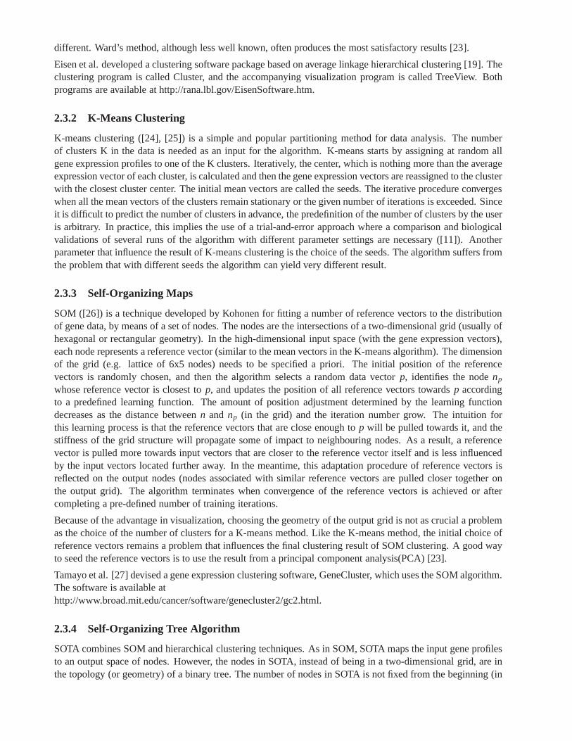
different. Ward’s method, although less well known, often produces the most satisfactory results [23].
Eisen et al. developed a clustering software package based on average linkage hierarchical clustering [19]. Theclustering program is called Cluster, and the accompanyingvisualization program is called TreeView. Bothprograms are available at http://rana.lbl.gov/EisenSoftware.htm.
2.3.2 K-Means Clustering
K-means clustering ([24], [25]) is a simple and popular partitioning method for data analysis. The numberof clusters K in the data is needed as an input for the algorithm. K-means starts by assigning at random allgene expression profiles to one of the K clusters. Iteratively, the center, which is nothing more than the averageexpression vector of each cluster, is calculated and then the gene expression vectors are reassigned to the clusterwith the closest cluster center. The initial mean vectors are called the seeds. The iterative procedure convergeswhen all the mean vectors of the clusters remain stationary or the given number of iterations is exceeded. Sinceit is difficult to predict the number of clusters in advance, the predefinition of the number of clusters by the useris arbitrary. In practice, this implies the use of a trial-and-error approach where a comparison and biologicalvalidations of several runs of the algorithm with differentparameter settings are necessary ([11]). Anotherparameter that influence the result of K-means clustering isthe choice of the seeds. The algorithm suffers fromthe problem that with different seeds the algorithm can yield very different result.
2.3.3 Self-Organizing Maps
SOM ([26]) is a technique developed by Kohonen for fitting a number of reference vectors to the distributionof gene data, by means of a set of nodes. The nodes are the intersections of a two-dimensional grid (usually ofhexagonal or rectangular geometry). In the high-dimensional input space (with the gene expression vectors),each node represents a reference vector (similar to the meanvectors in the K-means algorithm). The dimensionof the grid (e.g. lattice of 6x5 nodes) needs to be specified a priori. The initial position of the referencevectors is randomly chosen, and then the algorithm selects arandom data vectorp, identifies the nodenp
whose reference vector is closest top, and updates the position of all reference vectors towardsp accordingto a predefined learning function. The amount of position adjustment determined by the learning functiondecreases as the distance betweenn and np (in the grid) and the iteration number grow. The intuition forthis learning process is that the reference vectors that areclose enough top will be pulled towards it, and thestiffness of the grid structure will propagate some of impact to neighbouring nodes. As a result, a referencevector is pulled more towards input vectors that are closer to the reference vector itself and is less influencedby the input vectors located further away. In the meantime, this adaptation procedure of reference vectors isreflected on the output nodes (nodes associated with similarreference vectors are pulled closer together onthe output grid). The algorithm terminates when convergence of the reference vectors is achieved or aftercompleting a pre-defined number of training iterations.
Because of the advantage in visualization, choosing the geometry of the output grid is not as crucial a problemas the choice of the number of clusters for a K-means method. Like the K-means method, the initial choice ofreference vectors remains a problem that influences the finalclustering result of SOM clustering. A good wayto seed the reference vectors is to use the result from a principal component analysis(PCA) [23].
Tamayo et al. [27] devised a gene expression clustering software, GeneCluster, which uses the SOM algorithm.The software is available athttp://www.broad.mit.edu/cancer/software/genecluster2/gc2.html.
2.3.4 Self-Organizing Tree Algorithm
SOTA combines SOM and hierarchical clustering techniques.As in SOM, SOTA maps the input gene profilesto an output space of nodes. However, the nodes in SOTA, instead of being in a two-dimensional grid, are inthe topology (or geometry) of a binary tree. The number of nodes in SOTA is not fixed from the beginning (in
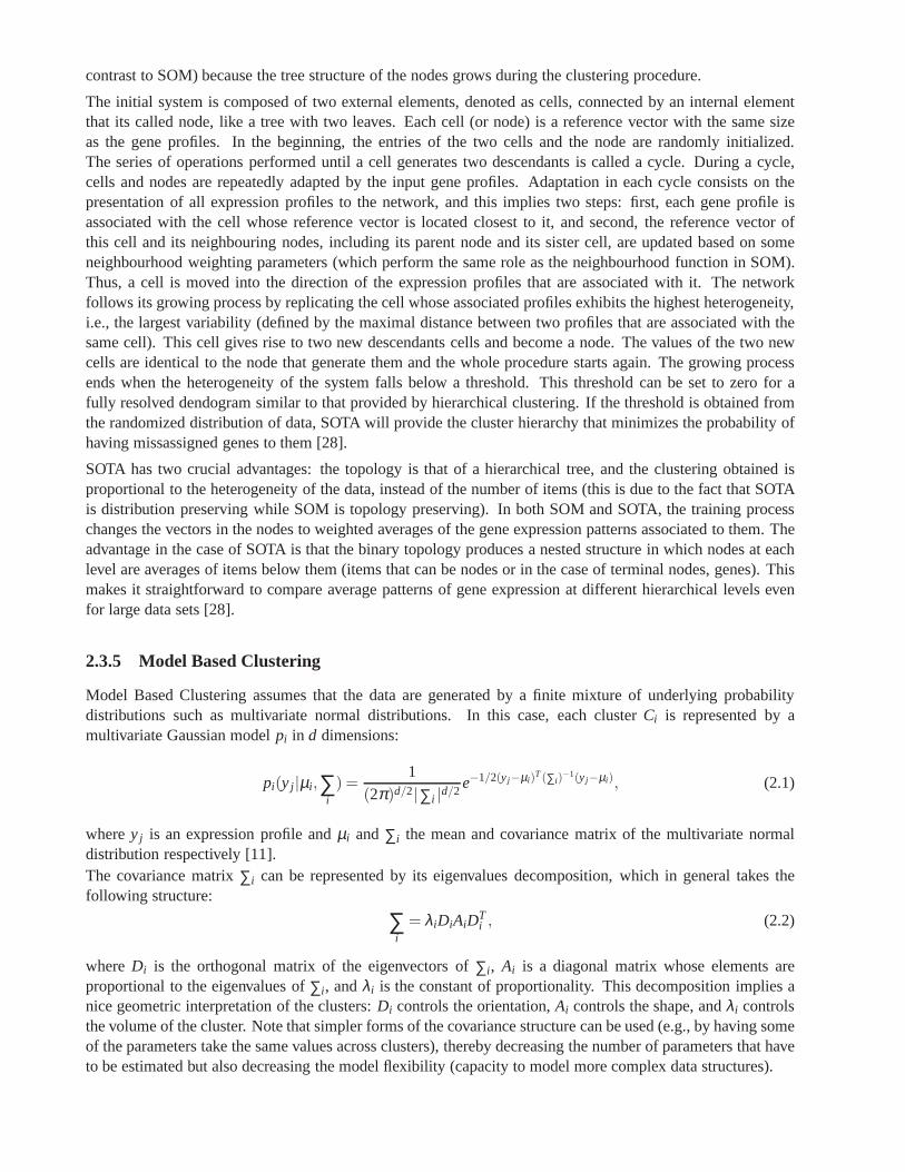
contrast to SOM) because the tree structure of the nodes grows during the clustering procedure.
The initial system is composed of two external elements, denoted as cells, connected by an internal elementthat its called node, like a tree with two leaves. Each cell (or node) is a reference vector with the same sizeas the gene profiles. In the beginning, the entries of the two cells and the node are randomly initialized.The series of operations performed until a cell generates two descendants is called a cycle. During a cycle,cells and nodes are repeatedly adapted by the input gene profiles. Adaptation in each cycle consists on thepresentation of all expression profiles to the network, and this implies two steps: first, each gene profile isassociated with the cell whose reference vector is located closest to it, and second, the reference vector ofthis cell and its neighbouring nodes, including its parent node and its sister cell, are updated based on someneighbourhood weighting parameters (which perform the same role as the neighbourhood function in SOM).Thus, a cell is moved into the direction of the expression profiles that are associated with it. The networkfollows its growing process by replicating the cell whose associated profiles exhibits the highest heterogeneity,i.e., the largest variability (defined by the maximal distance between two profiles that are associated with thesame cell). This cell gives rise to two new descendants cellsand become a node. The values of the two newcells are identical to the node that generate them and the whole procedure starts again. The growing processends when the heterogeneity of the system falls below a threshold. This threshold can be set to zero for afully resolved dendogram similar to that provided by hierarchical clustering. If the threshold is obtained fromthe randomized distribution of data, SOTA will provide the cluster hierarchy that minimizes the probability ofhaving missassigned genes to them [28].
SOTA has two crucial advantages: the topology is that of a hierarchical tree, and the clustering obtained isproportional to the heterogeneity of the data, instead of the number of items (this is due to the fact that SOTAis distribution preserving while SOM is topology preserving). In both SOM and SOTA, the training processchanges the vectors in the nodes to weighted averages of the gene expression patterns associated to them. Theadvantage in the case of SOTA is that the binary topology produces a nested structure in which nodes at eachlevel are averages of items below them (items that can be nodes or in the case of terminal nodes, genes). Thismakes it straightforward to compare average patterns of gene expression at different hierarchical levels evenfor large data sets [28].
2.3.5 Model Based Clustering
Model Based Clustering assumes that the data are generated by a finite mixture of underlying probabilitydistributions such as multivariate normal distributions.In this case, each clusterCi is represented by amultivariate Gaussian modelpi in d dimensions:
pi(y j |µi ,∑i) =
1
(2π)d/2|∑i |d/2e−1/2(yj−µi)
T(∑i)−1(yj−µi), (2.1)
wherey j is an expression profile andµi and∑i the mean and covariance matrix of the multivariate normaldistribution respectively [11].The covariance matrix∑i can be represented by its eigenvalues decomposition, whichin general takes thefollowing structure:
∑i
= λiDiAiDTi , (2.2)
whereDi is the orthogonal matrix of the eigenvectors of∑i , Ai is a diagonal matrix whose elements areproportional to the eigenvalues of∑i , andλi is the constant of proportionality. This decomposition implies anice geometric interpretation of the clusters:Di controls the orientation,Ai controls the shape, andλi controlsthe volume of the cluster. Note that simpler forms of the covariance structure can be used (e.g., by having someof the parameters take the same values across clusters), thereby decreasing the number of parameters that haveto be estimated but also decreasing the model flexibility (capacity to model more complex data structures).
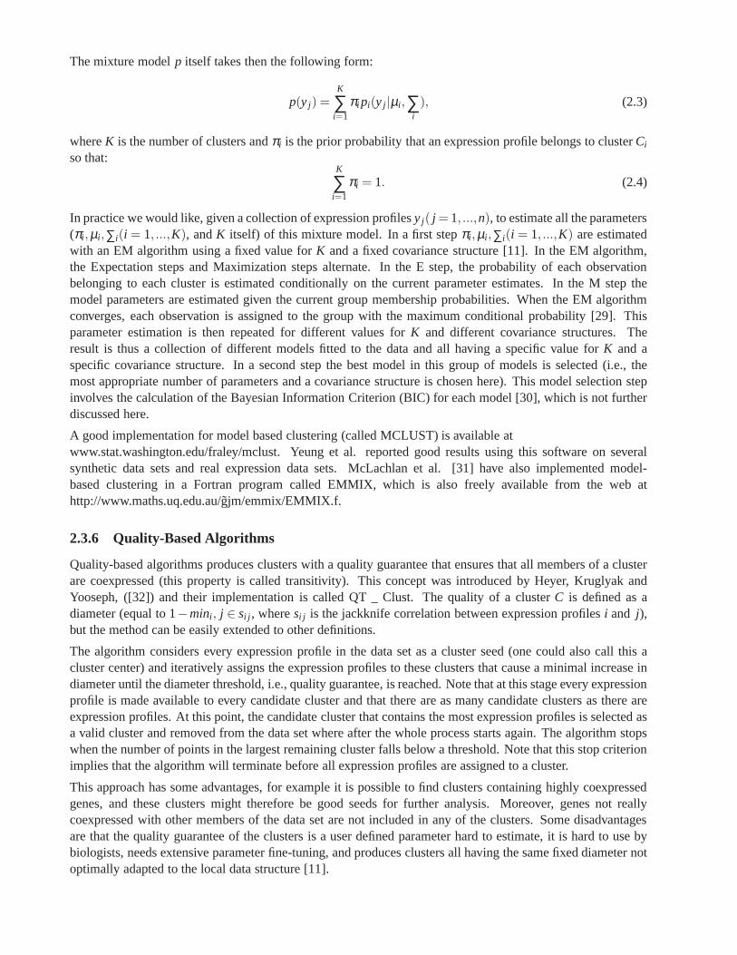
The mixture modelp itself takes then the following form:
p(y j) =K
∑i=1
πi pi(y j |µi ,∑i
), (2.3)
whereK is the number of clusters andπi is the prior probability that an expression profile belongs to clusterCi
so that:K
∑i=1
πi = 1. (2.4)
In practice we would like, given a collection of expression profilesy j( j = 1, ...,n), to estimate all the parameters(πi ,µi ,∑i(i = 1, ...,K), andK itself) of this mixture model. In a first stepπi ,µi ,∑i(i = 1, ...,K) are estimatedwith an EM algorithm using a fixed value forK and a fixed covariance structure [11]. In the EM algorithm,the Expectation steps and Maximization steps alternate. Inthe E step, the probability of each observationbelonging to each cluster is estimated conditionally on thecurrent parameter estimates. In the M step themodel parameters are estimated given the current group membership probabilities. When the EM algorithmconverges, each observation is assigned to the group with the maximum conditional probability [29]. Thisparameter estimation is then repeated for different valuesfor K and different covariance structures. Theresult is thus a collection of different models fitted to the data and all having a specific value forK and aspecific covariance structure. In a second step the best model in this group of models is selected (i.e., themost appropriate number of parameters and a covariance structure is chosen here). This model selection stepinvolves the calculation of the Bayesian Information Criterion (BIC) for each model [30], which is not furtherdiscussed here.
A good implementation for model based clustering (called MCLUST) is available atwww.stat.washington.edu/fraley/mclust. Yeung et al. reported good results using this software on severalsynthetic data sets and real expression data sets. McLachlan et al. [31] have also implemented model-based clustering in a Fortran program called EMMIX, which isalso freely available from the web athttp://www.maths.uq.edu.au/gjm/emmix/EMMIX.f.
2.3.6 Quality-Based Algorithms
Quality-based algorithms produces clusters with a qualityguarantee that ensures that all members of a clusterare coexpressed (this property is called transitivity). This concept was introduced by Heyer, Kruglyak andYooseph, ([32]) and their implementation is called QT _ Clust. The quality of a clusterC is defined as adiameter (equal to 1−mini , j ∈ si j , wheresi j is the jackknife correlation between expression profilesi and j),but the method can be easily extended to other definitions.
The algorithm considers every expression profile in the dataset as a cluster seed (one could also call this acluster center) and iteratively assigns the expression profiles to these clusters that cause a minimal increase indiameter until the diameter threshold, i.e., quality guarantee, is reached. Note that at this stage every expressionprofile is made available to every candidate cluster and thatthere are as many candidate clusters as there areexpression profiles. At this point, the candidate cluster that contains the most expression profiles is selected asa valid cluster and removed from the data set where after the whole process starts again. The algorithm stopswhen the number of points in the largest remaining cluster falls below a threshold. Note that this stop criterionimplies that the algorithm will terminate before all expression profiles are assigned to a cluster.
This approach has some advantages, for example it is possible to find clusters containing highly coexpressedgenes, and these clusters might therefore be good seeds for further analysis. Moreover, genes not reallycoexpressed with other members of the data set are not included in any of the clusters. Some disadvantagesare that the quality guarantee of the clusters is a user defined parameter hard to estimate, it is hard to use bybiologists, needs extensive parameter fine-tuning, and produces clusters all having the same fixed diameter notoptimally adapted to the local data structure [11].

2.3.7 Adaptive Quality-Based Clustering
Adaptive quality-based clustering ([33]) consist of a two-step approach. In the first step, a quality-basedapproach is performed to locate a cluster center in an area where the density of gene expression profiles islocally maximal using a preliminary estimate of the radius (i.e. the quality) of the cluster. In the secondstep, called adaptive step, the algorithm re-estimates theradius of the cluster so that the genes belonging to itare, in a statistical sense, significantly coexpressed. To this end, a bimodal and one-dimensional probabilitydistribution (the distribution consists of two terms: one for the cluster and one for the rest of the data) describingthe Euclidean distance between the data points and the cluster center is fitted to the data using an expectation-maximization (EM) algorithm.
Finally, step one and two are repeated, using the re-estimation of the quality as the initial estimate needed inthe first step, until the relative difference between the initial and re-estimated quality is sufficiently small. Thecluster is subsequently removed from the data and the whole procedure is restarted. Note that only clusterswhose size exceeds a predefined number are presented to the user.
In adaptive quality-based clustering, users have to specify a threshold for quality control. This parameter hasa strict statistical meaning and is therefore much less arbitrary (in contrast to the case in QT_Clust). It can bechosen independently of a specific data set or cluster and it allows for a meaningful default value (95%) thatin general gives good results. This makes the approach user friendly without the need for extensive parameterfine-tuning. Furthermore, with the ability to allow the clusters to have different radius, adaptive quality-basedclustering produces clusters adapted to the local data structure[11]. An application of Adaptive Quality- BasedClustering to nervous system is found in [34].
However, the method has some limitations like it does not converge in every situation. A server running theprogram is available at http://homes.esat.kuleuven.be/thijs/Work/Clustering.html
2.3.8 Biclustering and Some Physics Related Algorithms
Clustering can be applied to either the rows or the columns ofthe data matrix, separately. Biclustering, on theother hand, performs clustering in these two dimensions simultaneously. This means that clustering derives aglobal model while biclustering produces a local model[35]. The term biclustering was first used by Cheng andChurch [36] in gene expression data analysis. It refers to a distinct class of clustering algorithms that performsimultaneous row-column clustering. One of the earliest biclustering formulations is the direct clusteringalgorithm introduced by Hartigan [24], also known as block clustering.
The goal of biclustering techniques is thus to identify subgroups of genes and subgroups of conditions,by performing simultaneous clustering of both rows and columns of the gene expression matrix, insteadof clustering these two dimensions separately. We can then conclude that, unlike clustering algorithms,biclustering algorithms identify groups of genes that showsimilar activity patterns under a specific subsetof experimental conditions [35].
There are also several physics related clustering algorithms, e.g. Deterministic Annealing [37] and CoupledMass [38]. Deterministic Annealing uses the same cost function as K-means, but rather than minimizing itfor a fixed value of clusters K, it performs a statistical mechanics type analysis, using a maximum entropyprinciple as its starting point. The resulting free energy is a complex function of the number of centroids andtheir locations, which are calculated by a minimization process. This minimization is done by lowering thetemperature variable slowly and following minima that moveand every now and then split (corresponding toa second order phase transition). Since it has been proven [39] that in the generic case the free energy functionexhibits first order phase transitions, the deterministic annealing procedure is likely to follow one of its localminima [5].
Finally, it is important to stress that clustering methods have been used in a large variety of scientific disciplinesand applications that include pattern recognition [40], learning theory [41], astrophysics [42], medical imagesand data processing [43], machine translation of text [44],satellite data analysis [45], as well as speech
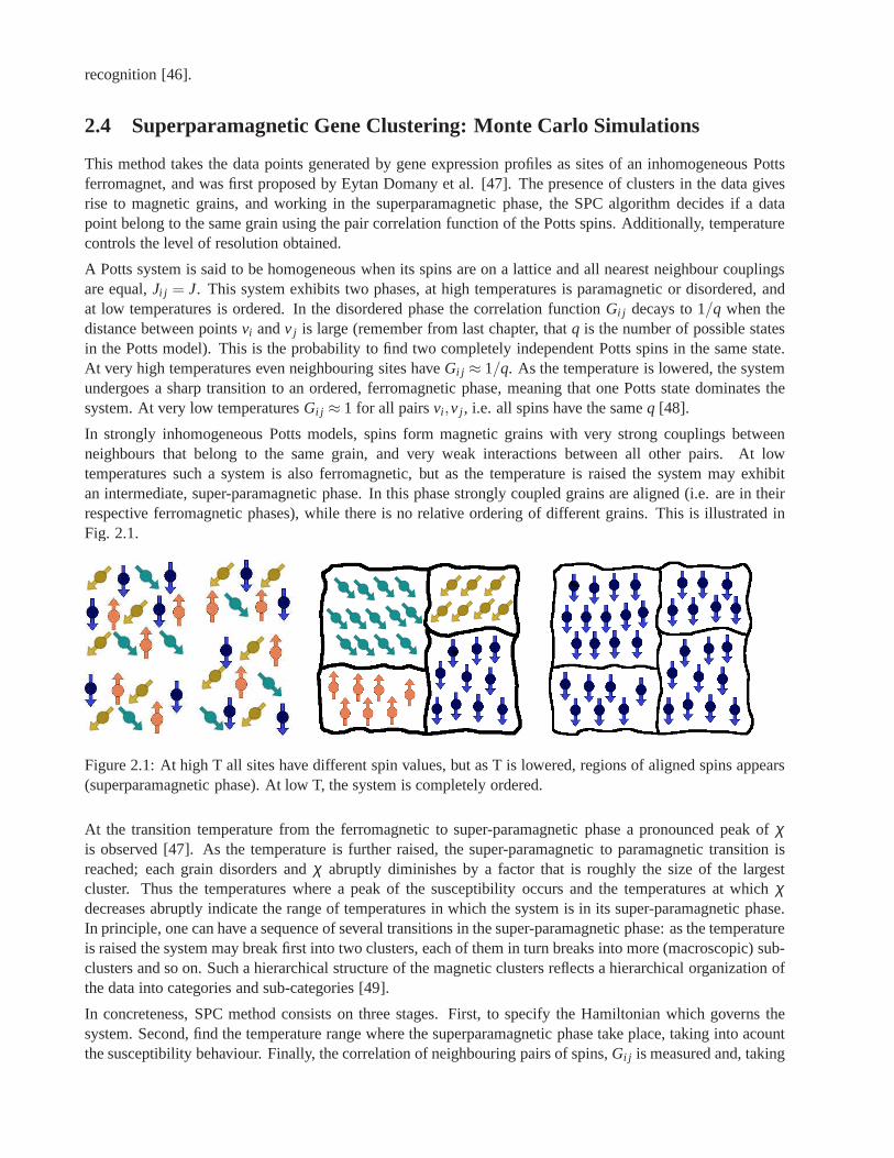
recognition [46].
2.4 Superparamagnetic Gene Clustering: Monte Carlo Simulations
This method takes the data points generated by gene expression profiles as sites of an inhomogeneous Pottsferromagnet, and was first proposed by Eytan Domany et al. [47]. The presence of clusters in the data givesrise to magnetic grains, and working in the superparamagnetic phase, the SPC algorithm decides if a datapoint belong to the same grain using the pair correlation function of the Potts spins. Additionally, temperaturecontrols the level of resolution obtained.
A Potts system is said to be homogeneous when its spins are on alattice and all nearest neighbour couplingsare equal,Ji j = J. This system exhibits two phases, at high temperatures is paramagnetic or disordered, andat low temperatures is ordered. In the disordered phase the correlation functionGi j decays to 1/q when thedistance between pointsvi andv j is large (remember from last chapter, thatq is the number of possible statesin the Potts model). This is the probability to find two completely independent Potts spins in the same state.At very high temperatures even neighbouring sites haveGi j ≈ 1/q. As the temperature is lowered, the systemundergoes a sharp transition to an ordered, ferromagnetic phase, meaning that one Potts state dominates thesystem. At very low temperaturesGi j ≈ 1 for all pairsvi ,v j , i.e. all spins have the sameq [48].
In strongly inhomogeneous Potts models, spins form magnetic grains with very strong couplings betweenneighbours that belong to the same grain, and very weak interactions between all other pairs. At lowtemperatures such a system is also ferromagnetic, but as thetemperature is raised the system may exhibitan intermediate, super-paramagnetic phase. In this phase strongly coupled grains are aligned (i.e. are in theirrespective ferromagnetic phases), while there is no relative ordering of different grains. This is illustrated inFig. 2.1.
Figure 2.1: At high T all sites have different spin values, but as T is lowered, regions of aligned spins appears(superparamagnetic phase). At low T, the system is completely ordered.
At the transition temperature from the ferromagnetic to super-paramagnetic phase a pronounced peak ofχis observed [47]. As the temperature is further raised, the super-paramagnetic to paramagnetic transition isreached; each grain disorders andχ abruptly diminishes by a factor that is roughly the size of the largestcluster. Thus the temperatures where a peak of the susceptibility occurs and the temperatures at whichχdecreases abruptly indicate the range of temperatures in which the system is in its super-paramagnetic phase.In principle, one can have a sequence of several transitionsin the super-paramagnetic phase: as the temperatureis raised the system may break first into two clusters, each ofthem in turn breaks into more (macroscopic) sub-clusters and so on. Such a hierarchical structure of the magnetic clusters reflects a hierarchical organization ofthe data into categories and sub-categories [49].
In concreteness, SPC method consists on three stages. First, to specify the Hamiltonian which governs thesystem. Second, find the temperature range where the superparamagnetic phase take place, taking into acountthe susceptibility behaviour. Finally, the correlation ofneighbouring pairs of spins,Gi j is measured and, taking
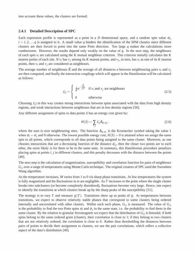
into account these values, the clusters are formed.
2.4.1 Detailed Description of SPC
Each expression profile is represented as a point in aD dimensional space, and a random spin valueσi,i = 1,2, ...,q is assigned to it. A small valueq hinders the identification of the SPM clusters since differentclusters are then forced to point into the same Potts direction. Too largeq makes the calculations morecumbersome. However, the results depend only weakly on the value ofq. In the next step, the neighboursof each spinvi are calculated using theK mutual neighbour criterion. This criterion initially calculates theKnearest points of each site. Ifvi hasv j among itsK nearest points, andv j , in turn, hasvi as one of itsK nearestpoints, thenvi andv j are considered as neighbours.
The average number of neighboursK and the average of all distancesa between neighbouring pairsvi andv j
are then computed, and finally the interaction couplings which will appear in the Hamiltonian will be calculatedas follows:
Ji j =
1K
e−d2i j
2a2 if vi andv j are neighbours
0 otherwise
(2.5)
ChoosingJi j in this way creates strong interactions between spins associated with the data from high densityregions, and weak interactions between neighbours that arein low density regions [50].
Any different assignment of spins to data pointsShas an energy cost given by:
H(S) = ∑i, j
Ji j δσi ,σ j , (2.6)
where the sum is over neighbouring sites. The functionδσi ,σ j is the Kroenecker symbol taking the value 1whenσi = σ j and 0 otherwise. The lowest possible energy cost,H(S) = 0 is attained when we assign the samespin to all points, which corresponds to all data points being assigned to the same cluster. Moreover, as onechooses interactions that are a decreasing function of the distancedi j , then the closer two points are to eachother, the more likely is for them to be in the same state. In summary, this Hamiltonian procedure penalizesplacing spins at pointsi, j in different clusters, and this penalty decreases with the distance between the points[49].
The next step is the calculation of magnetization, susceptibility and correlation function for pairs of neighboursGi j over a range of temperatures using Monte Carlo technique. The original creators of SPC used the SwendsenWang algorithm.
As the temperature increases,M varies from 1 to 0 via sharp phase transitions. At low temperatures the systemis fully magnetized and the fluctuations inmare negligible. AsT increases to the point where the single clusterbreaks into subclusters (or become completely disordered), fluctuations become very large. Hence, one expectto identify the transitions at which clusters break up by thesharp peaks of the susceptibility [51].
The strategy is to varyT and measureχ(T). Transitions show up as peaks ofχ . At temperatures betweentransitions, we expect to observe relatively stable phasesthat correspond to some clusters being orderedinternally and uncorrelated with other clusters. Within each such phase,Gi j is measured. The value ofGi j
is the probability to find the two Potts spinsσi andσ j in the same state, i.e. the probability to find them in thesame cluster. By the relation to granular ferromagnets we expect that the distribution ofGi j is bimodal; if bothspins belong to the same ordered grain (cluster), their correlation is close to 1; if they belong to two clustersthat are not relatively ordered, the correlation is close to0. Rather than thresholding the distances betweenpairs of points to decide their assignment to clusters, we use the pair correlations, which reflect a collectiveaspect of the data’s distribution [49].

Clusters are identified in three steps:
1. Build the cores of the clusters using a thresholding procedure. If Gi j > 0.5, a link is set between theneighbour data pointsvi andv j . The resulting connected graph depends weakly in the value used in thisthresholding, as long as it is bigger than 1/q and less than 1−2/q [49]. The reason is that the distributionof the correlations between two neighbouring spins peaks strongly at these two values and is very smallbetween them.
2. Capture points lying in the periphery by linking each point to its neighbour of maximal correlation. Ofcourse, some points were already linked in step one.
3. Data clusters are identified as the linked components of the graph obtained in the previous steps.
The temperature controls the resolution at which the data are clustered.It is intuitively clear that if a set of data points form a dense cloud, isolated from the rest of the data,the corresponding spins will form a ferromagnetic domain atsome low temperature, which will becomeparamagnetic and lose its correlations only at a high temperature. Hence the size of the temperature intervaldT in which such a ferromagnetic domain exists can be used as a measure of the stability and significance ofthe corresponding data cluster.Some of the demonstrated useful properties of SPC are the following: (a) the number of clusters is determinedby the algorithm itself and not externally prescribed (as isdone by SOM and K-means); (b) presents stabilityagainst noise; (c) generates a hierarchy (dendrogram) and provides a mechanism to identify in it robust, stableclusters (by the value of dT ); (d) ability to identify a denseset of points forming a cloud of an irregular (non-spherical shape) as a cluster [5].
The SPC method has been used in various contexts, like computer vision [52], speech recognition [49] andidentification of clusters of companies in stock indices [53]. Its first direct application to gene expression datahas been for analysis of the temporal dependence of the expression levels in a synchronized yeast culture [54],identifying gene clusters whose variation reflects the cellcycle. Subsequently, the SPC was used to identifyprimary targets of p53 [55], the most important tumour suppressor that acts as a transcription factor of centralimportance in human cancer. SPC has been used also to clusterprotein sequences [56], and to classify oridentify new genes associated with colon and skin cancer [57].
2.4.2 Future Directions
The location of the superparamagnetic phase in the SPC algorithm is closely related to the phase transitionsoccurring in the system. The introduction of the Wolff algorithm instead of the originally used Swendsen-Wang algorithm will probably improve the efficiency of the method, and this is left for future investigations,as well as a comparison of different methods with the SPC algorithm.

Chapter 3
Gompertz Equation
Contents
3.1 History of Gompertz Equation . . . . . . . . . . . . . . . . . . . . . . .. . . . . . . . . 50
3.2 Tumour Growth Equations . . . . . . . . . . . . . . . . . . . . . . . . . . .. . . . . . . 54
3.2.1 Exponential Growth . . . . . . . . . . . . . . . . . . . . . . . . . . . . .. . . . . 55
3.2.2 Logistic Growth . . . . . . . . . . . . . . . . . . . . . . . . . . . . . . . .. . . . 57
3.2.3 Von Bertalanffy Growth . . . . . . . . . . . . . . . . . . . . . . . . . .. . . . . . 59
3.2.4 Gompertz-Makeham Growth . . . . . . . . . . . . . . . . . . . . . . . .. . . . . . 60
3.2.5 Mathematical Properties and Comparison Between Logistic and Gompertz Growth . 61
49
3.1 History of Gompertz Equation
In 1724 Moivre presented his hypothesis of uniform decrement, summarized in the expressiony(x) =K(w−x),wherey(x) represents the surviving persons with agex, K is the slope or velocity with which the populationdiminishes in the mortality table, andw is the maximum survival age for the population. The Moivre straightline was recommended for an age range between 12 and 86, in which it adjusted better. This linear hypothesiswas exceeded by Benjamin Gompertz, who believed in the existence of two general causes of mortality: chanceand the increasing inability of men to avoid death. Gompertztook into account only the biological causes, andhis hypothesis was based on the following idea: “Men resistance to death diminish with time in a proportionalrate” [1].
Benjamin Gompertz was a British mathematician interested,besides other subjects as astronomy, in theproblem of life insurances and mortality rates in the nineteenth century. He worked with death and populationrecords of people in England, Sweden and France between ages20 and 60 and noted that the arithmeticincreases in age were consistently accompanied by geometric increases in mortality, and that this law ofgeometrical progression appeared in large portions of the different tables of mortality. Nowadays, the simpleformula describing the exponential rise in death rates between sexual maturity and extreme old age,γ(t) = eγt
is better known as Gompertz equation. In his first paper aboutthis subject published in 1820 [2], Gompertzidentified this peculiar pattern among different european populations for a limited portion of the age range. Forhis second paper, Gompertz used equal intervals of longer periods of time than in his previous work and found,for example, that the differences in the natural logarithm between successive 10 year age intervals betweenages 15 and 55 in a mortality table for Deparceaux, France, were all nearly identical. Gompertz believedhe had discovered a general law of mortality after observingsimilar patterns of geometrical progression inother tables of mortality, and published it in 1825 in the Philosophical Transactions of the Royal Society, ina paper whose title was “On the Nature of the Function Expressive of the Law of Human Mortality” [3]. Inhis third paper he improved his original notation and finallypresented the last one in 1860, published after hisdeath, where he noted that in his primary equation for geometric progression, the parameters were supposed torepresent constant quantities for a very long term of years [4].
From 1825 to 1862 Gompertz was involved on the subject of whatwas calledvital statistics in an effortto understand why there were consistent age patterns of death among people. Gompertz assumed that humanbeings have certain powers of integration and that those powers could be divided into a principal or fundamentalpart and an auxiliary part responsible for the maintenance of the principal power of integration. This auxilarforce is some kind of recuperative force, a power to oppose destruction that the organisms lose in equalproportions in equal small intervals of time. Gompertz alsobelieved on the presence of powers destroyingthis auxiliary force and multiplied this hypothetical force against life by the population alive to estimate thenumber of deaths in the age interval. Gompertz realized thatif the force to destroy life operated equally oneveryone, then all individuals should have the same length of life, something he knew could not be true. As apossible explanation, Gompertz emphasized the importanceof chance in the timing with which death occurs.At that time the concept of genetic heterogeneity was not known, instead, Gompertz invoked chance to explainwhy members of a presumed homogeneous cohort die at different times [5].
After Gompertz death, the subject remained mostly unknown in the scientific community. In 1860, W. M.Makeham improved Gompertz law of mortality incorporating aterm due to chance in the equation. He notedthat the logarithms of the probabilities of living from Gompertz’s formula increased at a faster pace at higherage than at younger ages, so he developed a theory of partial forces of mortality that intended to explain this.Makeham linked the diseases associated with the diminutionof the vital power to specific organ systems -thelungs, heart, kidneys, stomach and liver, and brain. These diseases represented a significant portion of totalmortality at that time and worked well in solving the observed problem of greater increased forces of mortalityat older ages than at younger ages. His formula accurately portrayed the mortality experience of various humanpopulations between ages 10 and 95 [6].
Gompertz and Makeham recognized that the original Gompertzequation did not apply to the entire age range,

the formula was intended to apply only between the ages of 20 and 60. In fact, Gompertz suggested in his lastpaper that there are four distinct periods in the life span between which separate laws of mortality apply: birthto 12 months, 12 months to 20 years, 20 years to 60 years, and 60years to 100 years. Even within this rangehe recognized that his formula worked best “provided the intervals be not greater than certain limits.” Theapplicability of the Gompertz function to only a specified range within the life span have been recognized bymany researchers but still nowadays some researchers reject the entire Gompertz paradigm after finding that itdoes not apply to older ages for some organisms [5].
Scientists started searching biological explanations forGompertz’s law of mortality until the first years ofthe twentieth century, motivated in part by the fact that increases in mortality among nonhuman species alsofollowed Gompertz’s law for a large portion of their life span. Differences among species were assumed to bejust a matter of scale.
Brownlee (1919) suggested that mortality due to senescent causes should be expressed first at about age 12,become the dominant force of total mortality by age 30, and advance at an exponential rate from ages 12 to85. He also recognized that a law of mortality was likely to beobscured by nonsenescent mortality. Brownleeidentified a formula that accurately describes the rate of decay of substances subject to the action of organicferments (i.e., bacteria exposed to a disinfecting solution) which he believed produced a time dependent decayanalogous to the loss of vital power. He found that his formula corresponded to Makeham’s adjustment ofGompertz’s equation, leading him to the conclusion that life depends on the energy of certain substances in thebody, an energy which is gradually being destroyed throughout life [7].
Wright (1926) [8] appears to have first suggested the use of the Gompertz curve for biological growth.Following Wright, Davidson (1928) used the Gompertz curve to represent the growth in body weight of cattle[10]. Weymouth, McMillin and Rich (1931) used the Gompertz curve to represent the growth in shell size ofthe razor clam [9]. They stated that the curve also gives goodfits for the guinea pig and the rat. It must benoted that they have found necessary in their most extensiveseries, the use of two different curves to graduatethe first and second halves of their data. Weymouth and Thompson (1931) also applied the Gompertz curve tothe growth of the Pacific cockle [11]. Since then, a number of authors fitted Gompertz formula to growth datafor animals and organisms with remarkable success.
Already in 1934, Casey fitted the Gompertz model to tumour growth data and was followed by numerousauthors [12]. The general conclusion has been that the Gompertz law very well describes tumor growth, but abiological explanation for this success has not been found.
The first person who attempted to perform an interspecies comparison of mortality, in this case, the mortalityschedules ofDrosophila and humans, was Raymond Pearl. Pearl (1921) plotted the survival curves of USmales in 1910 on a scale with those of the longwinged maleDrosophila [13]. Although Pearl acknowledgedthe arbitrary nature of this comparison, particularly in the choice of the beginning age interval for both species,he demonstrated a remarkable similarity in the curves. In his second study (1922), Pearl refined his interspeciesapproach and found that the form of the distributions was fundamentally the same [14]. In addition, he foundthat humans had a higher life expectancy at every age relative to theDrosophila, a discovery that he attributed tohumans’ control over their environment. Pearl was the first to manipulate experimentally the living conditionsof his study populations to test the importance of accidental deaths on the survival curves. He was convincedthat his research would reveal a “fundamental biological law” of mortality for more than one species, but aftertwo decades of research using this scaling approach on an expanded repertoire of species, Pearl and Minor[15] emphatically declared that a universal law of mortality did not exist. Pearl and Minor identified whatMakeham had identified 68 years before as the main problem -the inability to partition total mortality into itsintrinsic and extrinsic causes of death.
In the 50’s, researchers turned to the use of radiation, which they thought was a method to acceleratesenescence, for understanding aging and making interspecies extrapolation of mortality risks. George Sacher(1950), a pioneer in this field, assumed that the effects of radiation combined additively with natural aging,without introducing new pathology [16]. Under this assumption, the Sacher model accounted for natural aging

by the inclusion of a simple linear time dependent term to theintegral lethality function for radiation injury. Heobserved that at low daily dose rates, the reciprocal difference in mean survival times for a control and for anirradiated population was proportional to the intensity ofexposure. In 1952 Austin Brues and George Sacherenvisioned injury as a process that disrupts the normal physiological oscillations about a mean homeostaticstate within an organism, and that there were lethal injuries that an organism could not tolerate. Brues andSacher noted that this biological model of injury and failure lead directly to the formulation Gompertz derivedto describe his law of human mortality [17]. Using mean survival times, Sacher estimated cumulant lethalityfunctions to compare empirically the similarities and differences in species’ responses to radiation injury withinphases of the injury process. Sacher and Trucco, however, noted that they had insufficient knowledge about thefluctuation process in real systems and that the very fact of performing an observation introduced a disturbancein the study [18].
Like Brody before him, Failla (1958) definedvitality as the reciprocal of the age specific mortality rate [19].After expressing the Gompertz function in terms of vitality, he suggested that the resulting equation describedthe loss of vitality from a one hit random process acting on the cell population. Failla concluded that thevitality curve must describe a deterioration in the function of cells with age. He attributed the deterioration offunction to somatic mutations, and interpreted the Gompertz aging parameter (derived from mortality data)as an estimate of the spontaneous somatic gene mutation rateper cell per year. With some assumptionsabout generation length and the number of genes in diploid cells, Failla (1960) calculations suggested thatthe mutation rate per generation was similar across species[20]. This would imply that the somatic mutationrate per unit time is higher in short-lived animals than in animals with longer life span.
Szilard (1959) also developed a theory on the nature of the aging process based on the concept of accumulatedsomatic damage [21]. Inherited mutations in somatic genes whose function is critical late in the life spanwas viewed as the major explanation for the different lengths of human beings’ life. Like Sacher’s lethalbound, Szilard envisioned death occurring when the fraction of somatic cells unaffected by mutation reacheda critical threshold. He suggested that the magnitude of life shortening following exposure to radiation shouldbe inversely related to the square root of the number of chromosomes of a species. As such, mice and humansshould experience a similar radiation-induced life shortening when expressed as a fraction of the life span.
The quantitative as well as the biological importance of theGompertz distribution was further enhanced bythe work of Bernard Strehler and Albert Mildvan (1960) [22],these investigators presented a Gompertz-basedtheory of mortality and aging that was based on disruptions of the homeostatic state of an organism. Theirapproach differed from that of Sacher in the functional formof the equations used to describe the disturbancesof the “ energetic environment” of an organism challenged bystress. Strehler also made several importantobservations of the biological effects of radiation compared to the effects of aging. He noted that (1) agingeffects are typically associated with post-mitotic cell whereas radiation primarily affects dividing cells; (2)radiation damage is primarily genetic whereas the effects of aging appear to be more broad spectrum; (3) somespecies (e.g., Drosophila) do not exhibit life shortening even after large doses of radiation; and (4) the doserequired to double the mortality rate (i.e., Gompertz slope) produces a much larger increase in the mutationrate. Based on this observations, Strehler rejected the notion that radiation acts through a general accelerationof the normal aging process.
Studies of radiation effects continued to make extensive use of the Gompertz distribution throughout the1960’s. Like Greenwood (1928) before him [23], Grahn (1970)proposed to use the ratio of Gompertz slopes toadjust for life span differences when making mortality comparison between species [24]. Grahn successfullyused this scaling approach to predict reductions in human life expectancy following radiation exposure fromdoses response relationships observed in mice.
It seems that within the field of radiation, extrapolation between species had some success, but this differs fromPearl’s conclusion that a fundamental law of mortality applying to various species does not exist. The reasonlies on the environmental conditions of the animals being compared, because Pearl’s studies were based on thecomparison with species that experienced high levels of exogenous mortality, and the laboratory animals used

in radiation studies came from controlled environments without predation and where infectious diseases wereminimized. These environmental conditions are far more similar to the sheltered environment and medicalattention received by humans, leading to a better comparison between species [5].
The modern development of biodemography originated with a series of articles published by Weiss andcolleagues [25]. Weiss (1990) recognized that the field of genetic epidemiology could provide insights intothe biological constraints influencing the shape of the mortality function in populations. Weiss’s merging ofthe fields of demography and genetics and his subsequent elaboration using principles of evolutionary biologyserved as a launching point for the latest developments in the field of biodemography.
For most species survival beyond the age of reproduction is an extremely rare event with most deaths for acohort occurring just after birth. At these ages the vast majority of deaths result from forces of mortality thatare unrelated with senescence (e.g., predation or diseases). In this hostile environments, early reproductionhas become an essential element in species’ reproductive strategies ([26]). Consistent patterns of growth anddevelopment observed within species suggest that the reproductive biology of organisms alive today representsa genetic legacy of responses to environmental conditions that prevailed during early evolutionary history ofeach species. The modern evolutionary theory of senescenceis based on the premise that selection is effectivein altering gene frequencies until the time before the end ofthe reproductive period. When the normally highforce of external mortality is controlled and survival beyond the end of reproductive period becomes a commonoccurrence, senescence and senescent-related diseases and disorders have the opportunity to be expressed.Because there are common forces (i.e., extrinsic mortality) responsible for molding species’reproductivestrategies, a common pattern of intrinsic mortality, an evolutionary imprint, may become visible when speciesare compared on a biologically comparable time scale. Carnes et al. [27] have argued that the timing ofgenetically determined processes such as growth and development are driven by a reproductive biology, moldedby the necessity of early reproduction, which in turn is driven by the normally high external force of mortality.If individual senescence is an inadvertent consequence of these developmental processes as predicted fromthe evolutionary theory of senescence, then age patterns ofintrinsic mortality in a population should also becalibrated to some element(s) of a species’s reproductive biology. These ideas have been introduced in variouscomputational models.
Recent mortality schedules reveal a morepure biological influence because the external causes of deathhave been dramatically reduced by medical and technological advances and almost everyone now lives tohis biological potential. At the same time, a greater understanding of biological processes has also allowed themodification of intrinsic mortality (e.g. medicine, treatments and operations) altering the survival trajectoriesof individuals whose intrinsic diseases have already been expressed. From this perspective, the biologicallife span of a specie is one based on a mortality schedule thatwould prevail in the absence of survival timemanufactured by medical or pharmaceutical intervention ofany kind - a view consistent with that of RaymondPearl. When enough members of a population benefit from thesemedical interventions, it is possible that thelife span of the population will exceed its biologically based limits. All past research on mortality suggeststhat Gompertz was right all along: there are biological reasons for why death occurs when it does, and a lawof mortality for many species may very well exists. Which is the limit imposed by this law of mortality forhumans, and the degree to which these limits can be manipulated is still subject of great interest [5].
The Gompertz equation was developed exclusively for human beings both as an empirical tool to describe theage pattern of death from all causes during a limited time frame, and as representing a law of mortality thatarises from inherent biological processes. Gompertz neverimagined that his equation would become a toolused in the analysis not only of failure time of organisms butalso of failure time of mechanical devices and inthe description of biological and tumour growth.
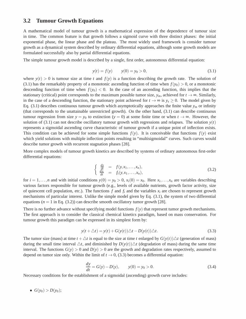
3.2 Tumour Growth Equations
A mathematical model of tumour growth is a mathematical expression of the dependence of tumour sizein time. The common feature is that growth follows a sigmoid curve with three distinct phases: the initialexponential phase, the linear phase and the plateau. The most widely used framework is consider tumourgrowth as a dynamical system described by ordinary differential equations, although some growth models areformulated successfully also by partial differential equations.
The simple tumour growth model is described by a single, firstorder, autonomous differential equation:
y(t) = f (y) y(0) = y0 > 0, (3.1)
wherey(t) > 0 is tumour size at timet and f (y) is a function describing the growth rate. The solution of(3.1) has the remarkably property of a monotonic ascending function of time whenf (y0)> 0, or a monotonicdescending function of time whenf (y0) < 0. In the case of an ascending function, this implies that thestationary (critical) point corresponds to the maximum possible tumor size,ym, achieved fort → ∞. Similarly,in the case of a descending function, the stationary point achieved fort → ∞ is ys ≥ 0. The model given byEq. (3.1) describes continuous tumour growth which asymptotically approaches the finite valueym or infinity(that corresponds to the unattainable unrestricted growth). On the other hand, (3.1) can describe continuoustumour regression from sizey = y0 to extinction (y = 0) at some finite time or whent → ∞. However, thesolution of (3.1) can not describe oscillatory tumour growth with regressions and relapses. The solutiony(t)represents a sigmoidal ascending curve characteristic of tumour growth if a unique point of inflection exists.This condition can be achieved for some simple functionsf (y). It is conceivable that functionsf (y) existwhich yield solutions with multiple inflection points resulting in “multisigmoidal” curves. Such curves woulddescribe tumor growth with recurrent stagnation phases [28].
More complex models of tumour growth kinetics are describedby systems of ordinary autonomous first-orderdifferential equations:
{ dydt = f (y,x1, . . . ,xn),
dxidt = fi(y,x1, . . . ,xn),
(3.2)
for i = 1, . . . ,n and with initial conditionsy(0) = y0 > 0, xi(0) = x0. Herexi , . . . ,xn are variables describingvarious factors responsible for tumour growth (e.g., levels of available nutrients, growth factor activity, sizeof quiescent cell population, etc.). The functionsf and fi and the variablesxi are chosen to represent growthmechanisms of particular interest. Unlike the simple modelgiven by Eq. (3.1), the system of two differentialequations (n= 1 in Eq. (3.2)) can describe smooth oscillatory tumor growth[28].
There is no further advance without specifying model functions f (y) that represent tumor growth mechanisms.The first approach is to consider the classical chemical kinetics paradigm, based on mass conservation. Fortumour growth this paradigm can be expressed in its simplestform by:
y(t +△t) = y(t)+G(y(t))△t −D(y(t))△t. (3.3)
The tumor size (mass) at timet +△t is equal to the size at timet enlarged byG(y(t))△t (generation of mass)during the small time interval△t, and diminished byD(y(t))△t (degradation of mass) during the same timeinterval. The functionsG(y) > 0 andD(y) > 0 are the growth and degradation rates respectively, assumed todepend on tumor size only. Within the limit oft → 0, (3.3) becomes a differential equation:
dydt
= G(y)−D(y), y(0) = y0 > 0. (3.4)
Necessary conditions for the establishment of a sigmoidal (ascending) growth curve includes:
• G(y0)> D(y0);
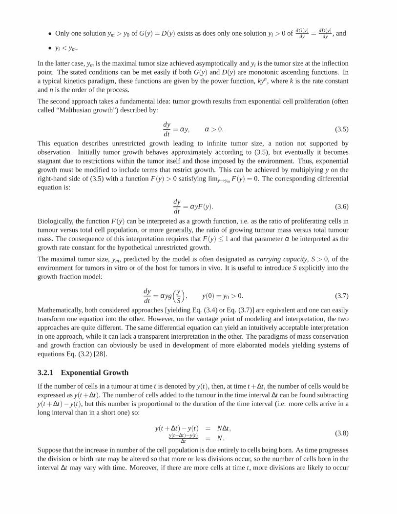
• Only one solutionym > y0 of G(y) = D(y) exists as does only one solutionyi > 0 of dG(y)dy = dD(y)
dy , and
• yi < ym.
In the latter case,ym is the maximal tumor size achieved asymptotically andyi is the tumor size at the inflectionpoint. The stated conditions can be met easily if bothG(y) andD(y) are monotonic ascending functions. Ina typical kinetics paradigm, these functions are given by the power function,kyn, wherek is the rate constantandn is the order of the process.
The second approach takes a fundamental idea: tumor growth results from exponential cell proliferation (oftencalled “Malthusian growth”) described by:
dydt
= αy, α > 0. (3.5)
This equation describes unrestricted growth leading to infinite tumor size, a notion not supported byobservation. Initially tumor growth behaves approximately according to (3.5), but eventually it becomesstagnant due to restrictions within the tumor itself and those imposed by the environment. Thus, exponentialgrowth must be modified to include terms that restrict growth. This can be achieved by multiplyingy on theright-hand side of (3.5) with a functionF(y) > 0 satisfying limy→ym F(y) = 0. The corresponding differentialequation is:
dydt
= αyF(y). (3.6)
Biologically, the functionF(y) can be interpreted as a growth function, i.e. as the ratio of proliferating cells intumour versus total cell population, or more generally, theratio of growing tumour mass versus total tumourmass. The consequence of this interpretation requires thatF(y)≤ 1 and that parameterα be interpreted as thegrowth rate constant for the hypothetical unrestricted growth.
The maximal tumor size,ym, predicted by the model is often designated ascarrying capacity, S> 0, of theenvironment for tumors in vitro or of the host for tumors in vivo. It is useful to introduceSexplicitly into thegrowth fraction model:
dydt
= αyg( y
S
)
, y(0) = y0 > 0. (3.7)
Mathematically, both considered approaches [yielding Eq.(3.4) or Eq. (3.7)] are equivalent and one can easilytransform one equation into the other. However, on the vantage point of modeling and interpretation, the twoapproaches are quite different. The same differential equation can yield an intuitively acceptable interpretationin one approach, while it can lack a transparent interpretation in the other. The paradigms of mass conservationand growth fraction can obviously be used in development of more elaborated models yielding systems ofequations Eq. (3.2) [28].
3.2.1 Exponential Growth
If the number of cells in a tumour at timet is denoted byy(t), then, at timet+∆t, the number of cells would beexpressed asy(t+∆t). The number of cells added to the tumour in the time interval∆t can be found subtractingy(t +∆t)−y(t), but this number is proportional to the duration of the time interval (i.e. more cells arrive in along interval than in a short one) so:
y(t +∆t)−y(t) = N∆t,y(t+∆t)−y(t)
∆t = N.(3.8)
Suppose that the increase in number of the cell population isdue entirely to cells being born. As time progressesthe division or birth rate may be altered so that more or less divisions occur, so the number of cells born in theinterval∆t may vary with time. Moreover, if there are more cells at timet, more divisions are likely to occur
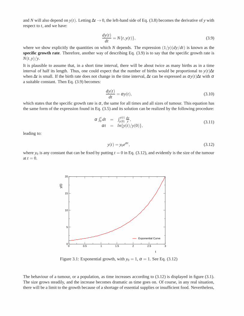
andN will also depend ony(t). Letting∆t → 0, the left-hand side of Eq. (3.8) becomes the derivative ofy withrespect tot, and we have:
dy(t)dt
= N{t,y(t)}, (3.9)
where we show explicitly the quantities on whichN depends. The expression(1/y)(dy/dt) is known as thespecific growth rate. Therefore, another way of describing Eq. (3.9) is to say that the specific growth rate isN(t,y)/y.
It is plausible to assume that, in a short time interval, there will be about twice as many births as in a timeinterval of half its length. Thus, one could expect that the number of births would be proportional toy(t)∆twhen∆t is small. If the birth rate does not change in the time interval, ∆t can be expressed asαy(t)∆t with αa suitable constant. Then Eq. (3.9) becomes:
dy(t)dt
= αy(t), (3.10)
which states that the specific growth rate isα , the same for all times and all sizes of tumour. This equationhasthe same form of the expression found in Eq. (3.5) and its solution can be realized by the following procedure:
α∫ t
0 dt =∫ y(t)
y(0)dyy ,
αt = ln{y(t)/y(0)},(3.11)
leading to:
y(t) = y0eαt , (3.12)
wherey0 is any constant that can be fixed by puttingt = 0 in Eq. (3.12), and evidently is the size of the tumourat t = 0.
0 0.5 1 1.5 2 2.5 3
t
0
5
10
15
20
y(t)
Exponential Curve
Figure 3.1: Exponential growth, withy0 = 1, α = 1. See Eq. (3.12)
The behaviour of a tumour, or a population, as time increasesaccording to (3.12) is displayed in figure (3.1).The size grows steadily, and the increase becomes dramatic as time goes on. Of course, in any real situation,there will be a limit to the growth because of a shortage of essential supplies or insufficient food. Nevertheless,
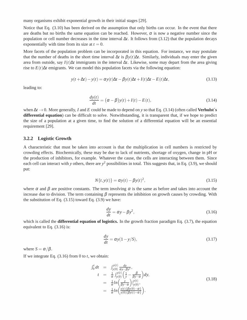
many organisms exhibit exponential growth in their initialstages [29].
Notice that Eq. (3.10) has been derived on the assumption that only births can occur. In the event that thereare deaths but no births the same equation can be reached. However,α is now a negative number since thepopulation or cell number decreases in the time interval∆t. It follows from (3.12) that the population decaysexponentially with time from its size att = 0.
More facets of the population problem can be incorporated inthis equation. For instance, we may postulatethat the number of deaths in the short time interval∆t is βy(t)∆t. Similarly, individuals may enter the givenarea from outside, sayI(t)∆t immigrants in the interval∆t. Likewise, some may depart from the area givingrise toE(t)∆t emigrants. We can model this population facets via the following equation:
y(t +∆t)−y(t) = αy(t)∆t −βy(t)∆t + I(t)∆t −E(t)∆t, (3.13)
leading to:
dy(t)dt
=(
α −β)
y(t)+ I(t)−E(t), (3.14)
when∆t → 0. More generally,I andE could be made to depend ony so that Eq. (3.14) (often calledVerhulst´sdifferential equation) can be difficult to solve. Notwithstanding, it is transparent that, if we hope to predictthe size of a population at a given time, to find the solution ofa differential equation will be an essentialrequirement [29].
3.2.2 Logistic Growth
A characteristic that must be taken into account is that the multiplication in cell numbers is restricted bycrowding effects. Biochemically, these may be due to lack ofnutrients, shortage of oxygen, change in pH orthe production of inhibitors, for example. Whatever the cause, the cells are interacting between them. Sinceeach cell can interact withy others, there arey2 possibilities in total. This suggests that, in Eq. (3.9), weshouldput:
N{t,y(t)} = αy(t)−βy(t)2, (3.15)
whereα andβ are positive constants. The term involvingα is the same as before and takes into account theincrease due to division. The term containingβ represents the inhibition on growth causes by crowding. Withthe substitution of Eq. (3.15) toward Eq. (3.9) we have:
dydt
= αy−βy2, (3.16)
which is called thedifferential equation of logistics. In the growth fraction paradigm Eq. (3.7), the equationequivalent to Eq. (3.16) is:
dydt
= αy(1−y/S), (3.17)
whereS= α/β .
If we integrate Eq. (3.16) from 0 tot, we obtain:
∫ t0 dt =
∫ y(t)y(0)
dyαy−βy2 ,
t = 1α∫ y(t)
y(0)
(
1y −
ββy−α
)
dy,
= 1α ln
(
yβy−α
)
|y(t)y(0),
= 1α ln
(
y(t){βy(0)−α}y(0){βy(t)−α}
)
.
(3.18)
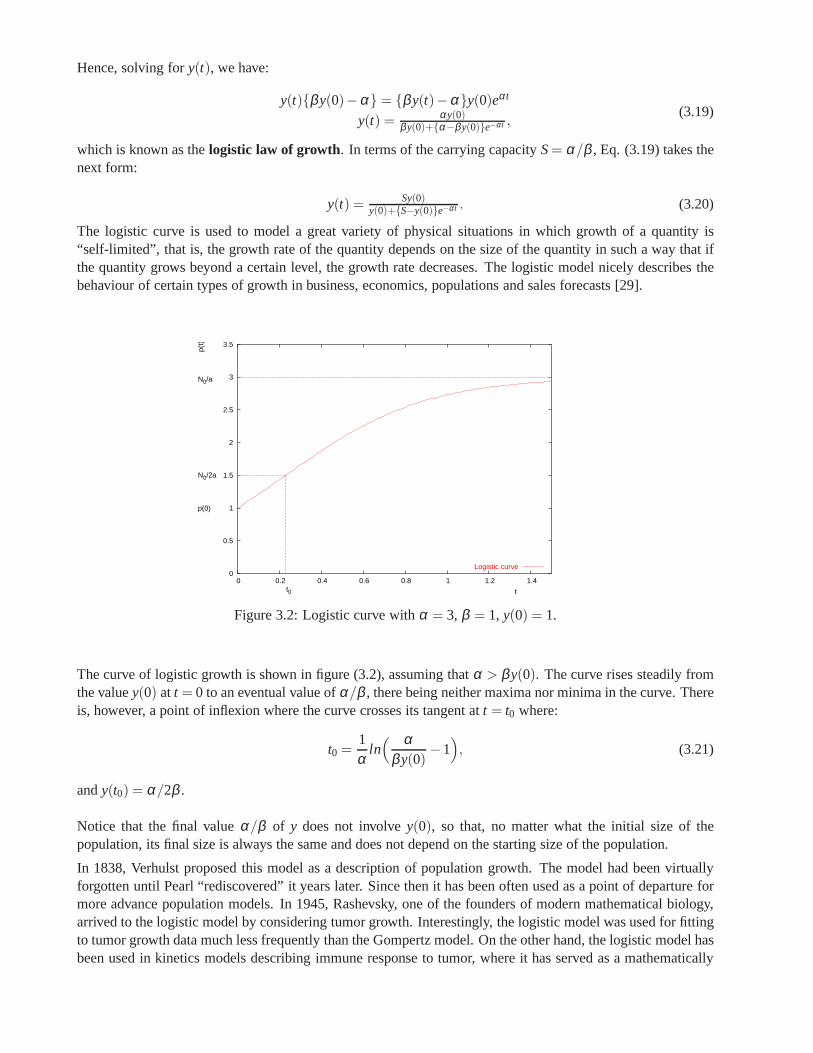
Hence, solving fory(t), we have:
y(t){βy(0)−α} = {βy(t)−α}y(0)eαt
y(t) = αy(0)βy(0)+{α−βy(0)}e−αt ,
(3.19)
which is known as thelogistic law of growth. In terms of the carrying capacityS= α/β , Eq. (3.19) takes thenext form:
y(t) = Sy(0)y(0)+{S−y(0)}e−αt . (3.20)
The logistic curve is used to model a great variety of physical situations in which growth of a quantity is“self-limited”, that is, the growth rate of the quantity depends on the size of the quantity in such a way that ifthe quantity grows beyond a certain level, the growth rate decreases. The logistic model nicely describes thebehaviour of certain types of growth in business, economics, populations and sales forecasts [29].
0
0.5
1
1.5
2
2.5
3
3.5
0 0.2 0.4 0.6 0.8 1 1.2 1.4
p(t)
t
N0/a
N0/2a
p(0)
t0
Logistic curve
Figure 3.2: Logistic curve withα = 3, β = 1, y(0) = 1.
The curve of logistic growth is shown in figure (3.2), assuming thatα > βy(0). The curve rises steadily fromthe valuey(0) at t = 0 to an eventual value ofα/β , there being neither maxima nor minima in the curve. Thereis, however, a point of inflexion where the curve crosses its tangent att = t0 where:
t0 =1α
ln( α
βy(0)−1
)
, (3.21)
andy(t0) = α/2β .
Notice that the final valueα/β of y does not involvey(0), so that, no matter what the initial size of thepopulation, its final size is always the same and does not depend on the starting size of the population.
In 1838, Verhulst proposed this model as a description of population growth. The model had been virtuallyforgotten until Pearl “rediscovered” it years later. Sincethen it has been often used as a point of departure formore advance population models. In 1945, Rashevsky, one of the founders of modern mathematical biology,arrived to the logistic model by considering tumor growth. Interestingly, the logistic model was used for fittingto tumor growth data much less frequently than the Gompertz model. On the other hand, the logistic model hasbeen used in kinetics models describing immune response to tumor, where it has served as a mathematically
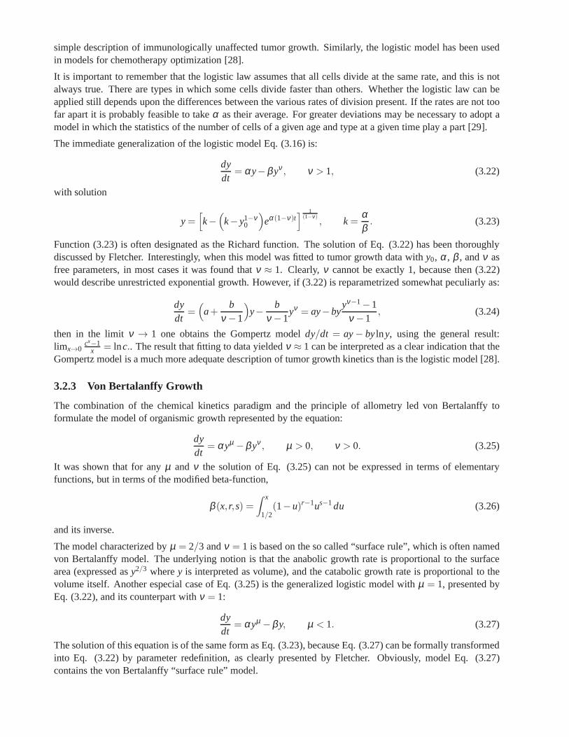
simple description of immunologically unaffected tumor growth. Similarly, the logistic model has been usedin models for chemotherapy optimization [28].
It is important to remember that the logistic law assumes that all cells divide at the same rate, and this is notalways true. There are types in which some cells divide faster than others. Whether the logistic law can beapplied still depends upon the differences between the various rates of division present. If the rates are not toofar apart it is probably feasible to takeα as their average. For greater deviations may be necessary toadopt amodel in which the statistics of the number of cells of a givenage and type at a given time play a part [29].
The immediate generalization of the logistic model Eq. (3.16) is:
dydt
= αy−βyν , ν > 1, (3.22)
with solution
y=[
k−(
k−y1−ν0
)
eα(1−ν)t]
1(1−ν)
, k=αβ. (3.23)
Function (3.23) is often designated as the Richard function. The solution of Eq. (3.22) has been thoroughlydiscussed by Fletcher. Interestingly, when this model was fitted to tumor growth data withy0, α , β , andν asfree parameters, in most cases it was found thatν ≈ 1. Clearly,ν cannot be exactly 1, because then (3.22)would describe unrestricted exponential growth. However,if (3.22) is reparametrized somewhat peculiarly as:
dydt
=(
a+b
ν −1
)
y− bν −1
yν = ay−byyν−1−1
ν −1, (3.24)
then in the limit ν → 1 one obtains the Gompertz modeldy/dt = ay− bylny, using the general result:limx→0
cx−1x = lnc.. The result that fitting to data yieldedν ≈ 1 can be interpreted as a clear indication that the
Gompertz model is a much more adequate description of tumor growth kinetics than is the logistic model [28].
3.2.3 Von Bertalanffy Growth
The combination of the chemical kinetics paradigm and the principle of allometry led von Bertalanffy toformulate the model of organismic growth represented by theequation:
dydt
= αyµ −βyν , µ > 0, ν > 0. (3.25)
It was shown that for anyµ and ν the solution of Eq. (3.25) can not be expressed in terms of elementaryfunctions, but in terms of the modified beta-function,
β (x, r,s) =∫ x
1/2(1−u)r−1us−1du (3.26)
and its inverse.
The model characterized byµ = 2/3 andν = 1 is based on the so called “surface rule”, which is often namedvon Bertalanffy model. The underlying notion is that the anabolic growth rate is proportional to the surfacearea (expressed asy2/3 wherey is interpreted as volume), and the catabolic growth rate is proportional to thevolume itself. Another especial case of Eq. (3.25) is the generalized logistic model withµ = 1, presented byEq. (3.22), and its counterpart withν = 1:
dydt
= αyµ −βy, µ < 1. (3.27)
The solution of this equation is of the same form as Eq. (3.23), because Eq. (3.27) can be formally transformedinto Eq. (3.22) by parameter redefinition, as clearly presented by Fletcher. Obviously, model Eq. (3.27)contains the von Bertalanffy “surface rule” model.
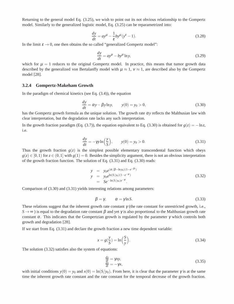
Returning to the general model Eq. (3.25), we wish to point out its not obvious relationship to the Gompertzmodel. Similarly to the generalized logistic model, Eq. (3.25) can be reparametrized into:
dydt
= ayµ − 1ε
byµ (yε −1). (3.28)
In the limit ε → 0, one then obtains the so called “generalized Gompertz model”:
dydt
= ayµ −byµ lny, (3.29)
which for µ = 1 reduces to the original Gompertz model. In practice, this means that tumor growth datadescribed by the generalized von Bertalanffy model withµ ≈ 1, ν ≈ 1, are described also by the Gompertzmodel [28].
3.2.4 Gompertz-Makeham Growth
In the paradigm of chemical kinetics (see Eq. (3.4)), the equation
dydt
= αy−βylny, y(0) = y0 > 0, (3.30)
has the Gompertz growth formula as the unique solution. The growth rateαy reflects the Malthusian law withclear interpretation, but the degradation rate lacks any such interpretation.
In the growth fraction paradigm (Eq. (3.7)), the equation equivalent to Eq. (3.30) is obtained forg(z) =− lnz,i.e.
dydt
=−γyln(y
S
)
, y(0) = y0 > 0. (3.31)
Thus the growth fractiong(z) is the simplest possible elementary transcendental function which obeysg(z) ∈ [0,1) for z∈ (0,1] with g(1) = 0. Besides the simplicity argument, there is not an obvious interpretationof the growth fraction function. The solution of Eq. (3.31) and Eq. (3.30) reads:
y = y0e(α/β−lny0)(1−e−β t)
y = y0eln(S/y0)(1−e−γt )
= Se− ln(S/y0)e−γt.
(3.32)
Comparison of (3.30) and (3.31) yields interesting relations among parameters:
β = γ , α = γ lnS. (3.33)
These relations suggest that the inherent growth rate constant γ (the rate constant for unrestricted growth, i.e.,S→ ∞ ) is equal to the degradation rate constantβ and yetγ is also proportional to the Malthusian growth rateconstantα . This indicates that the Gompertzian growth is regulated bythe parameterγ which controls bothgrowth and degradation [28].
If we start from Eq. (3.31) and declare the growth fraction a new time dependent variable:
x= g(yS) = ln
(Sy
)
. (3.34)
The solution (3.32) satisfies also the system of equations:
dydt = γxy,dxdt =−γx,
(3.35)
with initial conditionsy(0) = y0 andx(0) = ln(S/y0). From here, it is clear that the parameterγ is at the sametime the inherent growth rate constant and the rate constantfor the temporal decrease of the growth fraction.
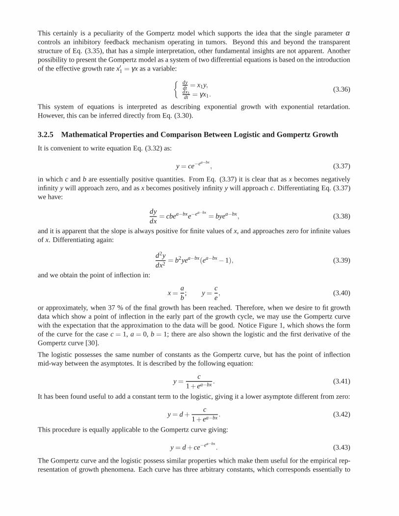
This certainly is a peculiarity of the Gompertz model which supports the idea that the single parameterαcontrols an inhibitory feedback mechanism operating in tumors. Beyond this and beyond the transparentstructure of Eq. (3.35), that has a simple interpretation, other fundamental insights are not apparent. Anotherpossibility to present the Gompertz model as a system of two differential equations is based on the introductionof the effective growth ratex′1 = γx as a variable:
{ dydt = x1y,dx1dt = γx1.
(3.36)
This system of equations is interpreted as describing exponential growth with exponential retardation.However, this can be inferred directly from Eq. (3.30).
3.2.5 Mathematical Properties and Comparison Between Logistic and Gompertz Growth
It is convenient to write equation Eq. (3.32) as:
y= ce−ea−bx, (3.37)
in which c andb are essentially positive quantities. From Eq. (3.37) it is clear that asx becomes negativelyinfinity y will approach zero, and asx becomes positively infinityy will approachc. Differentiating Eq. (3.37)we have:
dydx
= cbea−bxe−ea−bx= byea−bx, (3.38)
and it is apparent that the slope is always positive for finitevalues ofx, and approaches zero for infinite valuesof x. Differentiating again:
d2ydx2 = b2yea−bx(ea−bx−1), (3.39)
and we obtain the point of inflection in:
x=ab
; y=ce, (3.40)
or approximately, when 37 % of the final growth has been reached. Therefore, when we desire to fit growthdata which show a point of inflection in the early part of the growth cycle, we may use the Gompertz curvewith the expectation that the approximation to the data willbe good. Notice Figure 1, which shows the formof the curve for the casec = 1, a= 0, b = 1; there are also shown the logistic and the first derivative of theGompertz curve [30].
The logistic possesses the same number of constants as the Gompertz curve, but has the point of inflectionmid-way between the asymptotes. It is described by the following equation:
y=c
1+ea−bx. (3.41)
It has been found useful to add a constant term to the logistic, giving it a lower asymptote different from zero:
y= d+c
1+ea−bx. (3.42)
This procedure is equally applicable to the Gompertz curve giving:
y= d+ce−ea−bx. (3.43)
The Gompertz curve and the logistic possess similar properties which make them useful for the empirical rep-resentation of growth phenomena. Each curve has three arbitrary constants, which corresponds essentially to
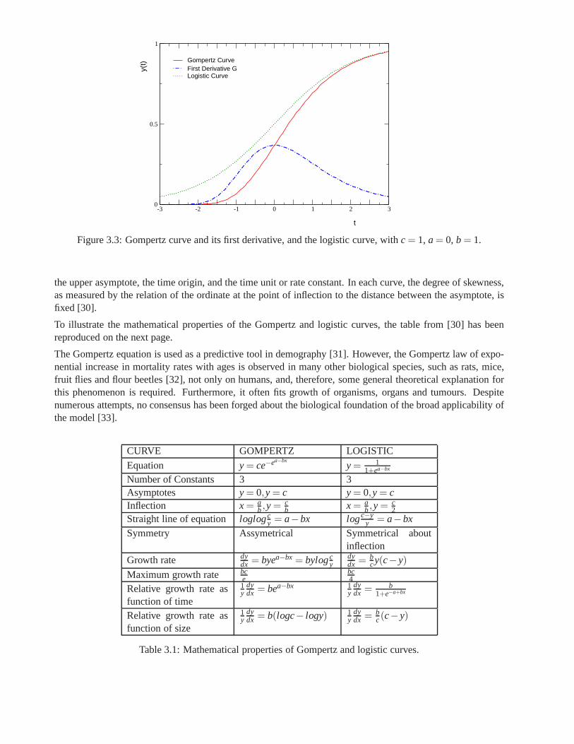
-3 -2 -1 0 1 2 3
t
0
0.5
1
y(t) Gompertz Curve
First Derivative GLogistic Curve
Figure 3.3: Gompertz curve and its first derivative, and the logistic curve, withc= 1, a= 0, b= 1.
the upper asymptote, the time origin, and the time unit or rate constant. In each curve, the degree of skewness,as measured by the relation of the ordinate at the point of inflection to the distance between the asymptote, isfixed [30].
To illustrate the mathematical properties of the Gompertz and logistic curves, the table from [30] has beenreproduced on the next page.
The Gompertz equation is used as a predictive tool in demography [31]. However, the Gompertz law of expo-nential increase in mortality rates with ages is observed inmany other biological species, such as rats, mice,fruit flies and flour beetles [32], not only on humans, and, therefore, some general theoretical explanation forthis phenomenon is required. Furthermore, it often fits growth of organisms, organs and tumours. Despitenumerous attempts, no consensus has been forged about the biological foundation of the broad applicability ofthe model [33].
CURVE GOMPERTZ LOGISTIC
Equation y= ce−ea−bxy= 1
1+ea−bx
Number of Constants 3 3Asymptotes y= 0,y= c y= 0,y= cInflection x= a
b,y=cb x= a
b,y=c2
Straight line of equation loglogcy = a−bx logc−y
y = a−bx
Symmetry Assymetrical Symmetrical aboutinflection
Growth rate dydx = byea−bx = bylogc
ydydx =
bcy(c−y)
Maximum growth rate bce
bc4
Relative growth rate asfunction of time
1y
dydx = bea−bx 1
ydydx =
b1+e−a+bx
Relative growth rate asfunction of size
1y
dydx = b(logc− logy) 1
ydydx =
bc(c−y)
Table 3.1: Mathematical properties of Gompertz and logistic curves.

Figure 3.4: A simple feedback control loop.
Appendix A: Control Theory Fundamentals
Control theory deals with the behaviour of dynamical systems over time. In a few words, is the mathematicalstudy of how to manipulate the parameters affecting the behaviour of a system to produce the desired or op-timal outcome. Control theory plays an important role in thedesign of manufacturing processes in industry,robotics, transportation, and biology, among other applications. Some of its basic concepts are the following:
System: set of elements that act in coordination to perform some objective.
Plant, P: is the physical element that one desires to control. Some examples are motors, ovens, navigationsystems, bioreactors, etc.
Output signal, y(t): is the variable that one wishes to control (position, velocity, pressure, temperature, etc).Is also called control variable.
Reference Signal,r(t): is the desired value for the output signal to reach.
Error, e(t): the difference between the reference signal and the real output signal.
Control signal, c(t): is the signal produced by the controllerC in order to modify the control variable in sucha way that the error decreases.
Process: steps that drive us to certain result.
Perturbation : a signal affecting the output of the system, deviating it from the desired value.
Sensor: device that turns the value of certain physical quantity (pressure, temperature, flow, etc.) into anelectrical signal codified in analogic or digital forms.
Closed-loop controller: the output of the systemy(t) is compared to the reference valuer(t), through themeasurement performed by a sensor. The controller then takes the difference between the reference and theoutput, the errore(t), to change the inputsu(t) to the system under control. Is known as feedback control.
Open-loop controller: the output signaly(t) is not monitored to generate a control signalc(t). There is nodirect connection between the output of the system and its input u(t). One of the main disadvantages of thistype of controller is the lack of sensitivity to the dynamicsof the system under control.
Stability : means that for any bounded input over any amount of time, theoutput will also be bounded. This isknown as BIBO stability. If a system is BIBO stable then the output cannot diverge if the input remains finite.
The most simple closed-loop controller is a so-called single-input-single-output (SISO) control system, andis presented in Fig. 3.4. Examples where one or more variables can contain more than a value (MIMO, i.e.Multi-Input-Multi-Output - for example when outputs to be controlled are two or more) are frequent. In suchcases variables are represented through vectors instead ofsimple scalar values.
If we assume the controllerC and the plantP are linear and time-invariant (i.e.: elements of their transferfunctionC(s) andP(s) do not depend on time), we can analyze the system shown in the Fig. 3.4 by using the
Laplace transform on the variables. This gives us the following relations:
Y(s) = P(s)U(s) (3.44)
U(s) =C(s)E(s) (3.45)
E(s) = R(s)−Y(s) (3.46)
Solving for Y(s) in terms of R(s), we obtain:
Y(s) =
(
P(s)C(s)1+P(s)C(s)
)
R(s) (3.47)
The term P(s)C(s)1+P(s)C(s) is referred to as the transfer function of the system. If we can ensureP(s)C(s)>> 1, i.e. it
has very great norm with each value ofs, thenY(s) is approximately equal toR(s). This means we control theoutput by simply setting the reference.
Controllability and observability are main issues in the analysis of system before decide the best controlstrategy to be applied.Controllability is related to the possibility to force the system in a particular stateby using an appropriate control signal. If a state is not controllable, then no signal will ever be able to forcethe system to reach a level of controllability.Observability instead is related to the possibility to“observe”,through output measurements, the system occupying a state.If a state is not observable, the controller willnever be able to correct the closed-loop behaviour if such a state is not desirable.
Every control system must guarantee first the stability of the closed-loop behaviour. For linear systems, thiscan be obtained directly placing the poles. The behaviour ofa non-linear system is not expressible as a linearfunction of its state or input variables, so non-linear control systems used instead specifical theories (normallybased on Lyapunov Theory) to ensure stability without regard to inner dynamics of the systems. The possibilityto fulfill different specifications varies from the model considered and/or the control strategy chosen.Solutions to problems of uncontrollable or unobservable system include adding actuators and sensors.
An observer is an auxiliary dynamical system which uses the available measurement on the system in order toprovide an estimate ˆx of the state of the system. The dynamical nature of an observer means that the estimatesof the state variable are provided on line. By anadaptive schemewe mean an observer that is able to providean estimate state even in face of parameter uncertainties.
http://en.wikipedia.org/wiki/Control_theory

Bibliography: Chapter 1
[1] R. Eckhardt,Stan Ulam, John Von Neumann, and the Monte Carlo Method, Los Alamos Science, Vol.15, 1987, p. 131.
[2] N. Metropolis,The Beginning of the Monte Carlo Method, Los Alamos Science, Vol. 15, 1987, p. 125.
[3] A. Hall, On an Experimental Determination ofπ, Messeng. Math., Vol. 2, 1873, p. 113.
[4] Lord Kelvin, Nineteenth Century Clouds Over the Dynamical Theory of Heatand Light, Phil. Mag.,Vol. 6, 1901, p. 1.
[5] H.L. Anderson,Metropolis, Monte Carlo, and the MANIAC, Los Alamos Science, Vol. 14, 1986, p. 96.
[6] N. Metropolis and S. Ulam,The Monte Carlo Method, Journal of the American Statistical Association,Vol. 44, 1949, p. 335.
[7] N. Metropolis, A. Rosenbluth, M. Rosenbluth, A. Teller and E. Teller,Equation of State Calculationsby Fast Computing Machines, The Journal of Chemical Physics, Vol. 21, 1953, p. 1087.
[8] M. Giersz, Monte Carlo Simulations of Star Clusters - II. Tidally Limited, Multi-mass Systems withStellar Evolution, Monthly Notices of the Royal Astronomical Society, Vol. 324, 2001, p. 218.arXiv:astro-ph/0103001
F. A. Rasio, J. M. Fregeau, and K. J. Joshi,Binaries and Globular Cluster Dynamics, in The Influenceof Binaries on Stellar Population Studies, ed. D. Vanbeveren (Dordrecht: Kluwer), 2001, p. 387.arXiv:astro-ph/0103001
[9] D. B. Graves, M. J. Kushner,Influence of Modeling and Simulation on the Maturation of PlasmaTechnology: Feature Evolution and Reactor Design, J. Vac. Sci. Technol. A, Vol. 21, 2003, p. S152.
J. L. Hutton, N. R. Smith,Use of a Monte Carlo Hybrid Technique for Power Shape Calculations,MC2000, International Conference on Advanced Monte Carlo for Radiation Physics, Particle TransportSimulation and Applications, Lisbon, Portugal, 2000.
[10] R. Spaic, R. Ilic, M. Dragovic, and B. Petrovic,Generation of Dose-Volume Histograms UsingMonte Carlo Simulations on a Multicellular Model in Radionuclide Therapy, Cancer Biotherapy andRadiopharmaceuticals, Mary Ann Liebert, Inc. Vol. 20, 2005.
C. M. Ma, E. Mok, A. Kapur, T. Pawlicki, D. Findley, S. Brain, K. Korster, and A. L. Boyer,ClinicalImplementation of a Monte Carlo Treatment Planning System, Med Phys, Vol. 26, 1999, p. 2133.
[11] A. L. Rodrigues and M. J. Oliveira,Continuous Time Stochastic Models for Vehicular Traffic onHighways, Braz. J. Phys., Vol.34, 2004, p. 373.
D. Chowdhury, K. Ghosh, A. Majumdar, S. Sinha, and R. B. Stinchcombe,Particle-hopping Modelsof Vehicular Traffic: Distributions of Distance Headways and Distance Between Jams, Physica A, Vol.246, 1997, p. 471. arXiv:cond-mat/9706094
65

[12] C. F. Kelliher and L. S. Mahoney,Using Monte Carlo Simulation to Improve Longterm InvestmentDecisions, The Appraisal Journal, Vol. 68, 2000, pp. 44-56.
W.J. Hurley, On the Use of Martingales in Monte Carlo Approaches to Multiperiod ParameterUncertainty in Capital Investment Risk Analysis, The Engineering Economist, Vol. 43, 1998, p. 169.http://www.findarticles.com/p/articles/mi_qa3621/is_199801/ai_n8786476
[13] E. A. Holm, G. N. Hassold and M. A. Miodownik,On Misorientation Distribution Evolution DuringAnisotropic Grain Growth, Acta mater., Vol. 49, 2001, p. 2981.
[14] A. Rollett and P. Manohar,Chapter 4: The Monte Carlo Method, in Continuum Scale Simulation ofEngineering Materials: Fundamentals - Microstructures - Process Applications, Wiley-VCH Verlag,2004, p. 76.
[15] D. S. Mainardi and P. B. Balbuena,Monte Carlo Simulation of Cu-Ni Nanoclusters: Surface SegregationStudies, Langmuir, Vol. 17, 2001, p. 2047.
Y. Kwon and D. Tománek,Orientational Melting in Carbon Nanotube Ropes, Phys. Rev. Let. Vol. 84,2000, p. 14.
V. H. Crespi, N. G. Chopra, M. L. Cohen, A. Zettl and V. Radmilovic, Site-selective Radiation Damageof Collapsed Carbon Nanotubes, Applied Physics Letters, Vol. 73, 1998, p. 2435.
[16] D. G. Covell,Folding Protein Alpha-Carbon Chains into Compact Forms by Monte Carlo Methods,Proteins: Structure, Function and Genetics, Vol. 14, 1992,p. 409.
A. Kolinski, P. Klein, P. Romiszowski, and J. Skolnicky,Unfolding of Globular Proteins: Monte CarloDynamics of a Realistic Reduced Model, Biophysical Journal, Vol. 85, 2003, p. 3271.
A. Irbäck, Hybrid Monte Carlo Simulation of Polymer Chains, The Journal of Chemical Physics, Vol.101, 1994, p. 1661.
A. Sikorski and P. Romiszowski,Monte Carlo Simulations of Protein-like Heteropolymers, ActaBiochimica Polonica, Vol. 48, 2001.
[17] D. P. Landau and K. Binder,A Guide to Monte Carlo Simulations in Statistical Physics, CambridgeUniversity Press, 2nd ed., 2002.
[18] C. Andrieu, N. de Freitas, A. Doucet, M. Jordan,An Introduction to MCMC for Machine Learning,Machine Learning, Vol. 50, 2003, p. 5.
[19] R. Sun,Cluster Algorithms for the Ising Model and the Widom-Rowlinson Model, chapter 1 and chapter2, thesis, 1998, Clark University.
[20] P. Coddington,http://www.npac.syr.edu/users/paulc/lectures/montecarlo/p_montecarlo.html
[21] E. Ising,Beitrag zur Theorie des Ferromagnetismus, Zeitschr. f. Physik, Vol. 31, 1925, p. 253.
[22] W. Lenz,Beitrag zum Verständnis der Magnetischen Eigenschaften inFesten Körpern, Phys. Zeitschr.,Vol. 21, 1920, p. 613.
[23] W. Heisenberg,Zur Theorie des Ferromagnetismus, Zeitschr. f. Physik, Vol. 49, 1928, p. 619.
[24] R. Peierls,On Ising’s Model of Ferromagnetism, Proc. Cambridge Phil. Soc., Vol. 32, 1936, p. 477.
[25] H. A. Kramers and G. H. Wannier,Statistics of the Two-Dimensional Ferromagnet. Part I, Phys. Rev.,Vol. 60, 1941, p. 252.

[26] L. Onsager,Crystal Statistics. I. A Two-Dimensional Model with a Order-Disorder Transition, Phys.Rev., Vol. 65, 1944, p. 117.
[27] http://scienceworld.wolfram.com/physics/IsingModel.html
[28] E. Marinari, G. Parisi and J.J. Ruiz-Lorenzo,Numerical Simulations of Spin Glass Systems, in SpinGlasses and Random Fields, edited by P. Young,(Singapore: World Scientific), 1997, p. 130. arXiv:cond-mat/9701016
[29] R. B. Potts,Some Generalized Order-Disorder Transformations, Proc. Camb. Phil. Soc. Vol. 48, 1952,p. 106.
[30] R. H. Swendsen and J. S. Wang,Nonuniversal Critical Dynamics in Monte Carlo Simulations, Phys.Rev. Lett., Vol.58, 1987, p. 86.
[31] U. Wolff, Collective Monte Carlo Updating for Spin Systems, Phys. Rev. Lett., Vol. 62, 1989, p. 361.
[32] http://en.wikipedia.org/wiki/Phase_transition
[33] http://www.absoluteastronomy.com/encyclopedia/p/ph/phase_(matter).htm
[34] chapter 3: Critical Phenomena and phase Transitionsin Condensed Matter Physics (Physics throughthe 1990s), National Academy Press, Washington D.C., 1986.http://www.nap.edu/books/0309035775/html/
[35] F.Y. Wu,The Potts Model, Rev. Mod. Phys., Vol. 54, 1982, p. 235.
[36] H. Gould, J. Tobochnik, and W. Christian,chapter 15: Monte Carlo Simulations of Thermal Systems,in Introduction to Computer Simulation Methods: Applications to Physical Systems, Addison-Wesley,3rd. ed., 2006.
[37] A. M. Ferrenberg and R. H. Swendsen,New Monte Carlo Technique for Studying Phase Transitions,Phys. Rev. Lett., Vol 61, 1988, p. 2635.
[38] Z. W. Salsburg, J. D. Jackson, W. Fickett and W. W. Wood,Application of Monte Carlo Method to theLattice Gas Model. I. Two dimensional Triangular Lattice, J. Chem. Phys., Vol. 30, 1959, p. 65.
D. A. Chesnut and Z. W. Salsburg,Monte Carlo Procedure for Statistical Mechanical Calculations in aGrand Canonical Ensemble of Lattice Systems, J. Chem. Phys., Vol. 38, 1963, p. 2861.
I. R. McDonald and K. Singer, Discuss. Faraday Soc., Vol. 43,1967, p. 40.
I. R. McDonald and K. Singer,Machine Calculation of Thermodynamic Properties of a Simple Fluid atSupercritical Temperature, J. Chem. Phys., Vol. 47, 1967, p. 4766.
I. R. McDonald and K. Singer,Estimation of the Adequacy of the 12-6 Potential for Liquid Argon byMeans of Monte Carlo Calculations, J. Chem. Phys., Vol. 50, 1969, p. 2308.
J. P. Valleau and D. N. Card,Monte Carlo Estimation of Free Energy by Multi-Stage Sampling, J. Chem.Phys., Vol. 57, 1972, p. 5457.
G. Bhanot, S. Black, P. Carter and R. Salvador,A New Method for the Partition Function of DiscreteSystems with Applications the 3D Ising Model, Phys. Lett. B, Vol. 183, 1987, p. 331.
G. Bhanot, K. M. Bitar, S. Black, P. Carter and R. Salvador,The Partition Function of Z(2) and Z(8)Lattice Gauge Theory in Four Dimensions, a Novel Approach toSimulations of Lattice Systems, Phys.Lett. B, Vol. 187, 1987, p. 381.
[39] G. Torrie and J. P. Valleau,Monte Carlo Free Energy Estimates Using Non- Boltzmann Sampling:Application to the Sub-Critical Lennard-Jones Fluid, Chem. Phys. Lett., Vol. 28, 1974, p. 578.

[40] K. Venu, V. S. S. Sastri and K. P. N. Murthy,Nematic - Isotropic Transition in Porous Media - A MonteCarlo Study, Europhys. Lett., Vol. 58, 2002, p. 646.
[41] A. M. Ferrenberg and D. P. Landau,Critical Behavior of the Three-Dimensional Ising Model: A HighResolution Monte Carlo Study, Phys. Rev. B, Vol.44, 1991, p. 5081.
[42] A. M. Ferrenberg and R. H. Swendsen,New Monte Carlo Data Analysis, Phys. Rev. Lett., Vol 63, 1989,p. 1195.
C. H. Bennet,Efficient Estimation of Free Energy Difference from Monte Carlo Data, J. Comput. Phys.,Vol. 22, 1976, p. 245.
N. A. Alves, B. A. Berg, and R. Villanova,Ising Model Monte Carlo Simulations: Density of States andMass Gap, Phys. Rev. B, Vol. 41, 1990, p. 383.
[43] B. A. Berg and T. Neuhaus,Multicanonical Algorithms for First Order Phase Transition, Phys. Lett. B,Vol. 267, 1991, p. 249.
B. A. Berg and T. Neuhaus,Multicanonical Ensemble: A New Approach to Simulation of First OrderPhase Transition, Phys. Rev. Lett., Vol. 68, 1992, p. 9.
[44] J. Lee and J. M. Kosterlitz,New Numerical Method to Study Phase Transition, Phys. Rev Lett., Vol. 65,1990, p. 137.
[45] S. Gupta,Finite-Size Scaling at Phase Coexistence, Nucl. Phys. B, Vol. 409, 1993, p. 663. arXiv:hep-lat/9305006
[46] K. Rummukainen, Lectures Notes, Finite Size Scaling
http://theory.physics.helsinki.fi/ xfiles/simu/03/
[47] J. C. Niel and J. Zinn-Justin,Finite Size Effects in Critical Dynamics, Nucl. Phys. B, Vol. 280, 1987, p.355.
K. Binder, Monte Carlo Calculation of the Surface Tension for Two- and Three-Dimensional Lattice-Gas Models, Phys. Rev. A, Vol. 25, 1982, p. 1699.
[48] Y. Iwasaki, K. Kanaya, Leo Kärkkäinen,K. Rummukainen,and T. Yoshié, Interface Tension inQuenched QCD, Phys. Rev. D, Vol. 49, 1994, p. 3540. arXiv:hep-lat/9309003
[49] M. E. Fisher and A. N. Berker,Scaling for First-Order Phase Transitions in Thermodynamic and FiniteSystems, Phys. Rev. B, Vol. 26, 1982, p. 2507.
[50] K. Binder and D. P. Landau,Finite-Size Scaling at First-Order Phase Transitions, Phys. Rev. B, Vol. 30,1984, p. 1477.
[51] M. S. Challa, D. P. Landau and K. Binder,Finite-Size Effects at Temperature-Driven First-OrderTransitions, Phys. Rev. B, Vol. 34, 1986, p. 1841.
[52] C. Borgs, R. Kotecký ,A Rigorous Theory of Finite Size Scaling at First Order PhaseTransitions, J.Stat. Phys., Vol. 61, 1990, p. 79.
[53] C. Borgs, R. Kotecký, S. Miracle-Solé ,Finite-Size Scaling for Potts Models, J. Stat. Phys., Vol. 62,1992, p. 529.
[54] A. Billoire, Nucl. Phys. (Proc. Suppl.), Vol. B42, 1995, p. 21.
[55] B. Ortakaya, Y. Gündüç, M. Aydin and T. Çelik,Scaling of Cluster Fluctuations in Two-Dimensional q= 5 and 7 State Potts Models, arXiv:hep-lat/9701017

[56] A. Billoire, R. Lacaze and A. Morel, Nucl. Phys., Vol. B370, 1992, p. 773.
[57] J. Lee and J. M. Kosterlitz,Finite-Size Scaling and Monte Carlo Simulations of First-Order PhaseTransition, Phys. Rev B, Vol. 43, 1991, p. 3265.
[58] K. Binder, Finite Size Scaling Analysis of Ising Model Block Distribution Functions, Z. Phys. B-Condensed Matter, Vol. 43, 1981, p. 119.
[59] M. E. Fisher,Critical Phenomena, ed. M.S. Green (Academic Press London).
M. E. Fisher and M. N. Barber,Scaling Theory for Finite-Size Effects in the Critical Region, Phys. RevLett. Vol. 28, 1972, p. 1516.
[60] A. M. Ferrenberg and R. H. Swendsen,Optimized Monte Carlo Data Analysis, Phys. Rev. Lett., Vol.63, 1989, p. 1195. C. H. Bennet,Efficient Estimation of Free Energy Difference from Monte Carlo Data,J. Comput. Phys., Vol. 22, 1976, p. 245. N. A. Alves, B. A. Berg, and R. Villanova, em Ising ModelMonte Carlo Simulations: Density of States and Mass Gap, Phys. Rev. B, Vol. 41, 1990, p. 383.
[61] A. Billoire, T. Neuhaus and B. Berg, Saclay preprint, 1992, SPhT-92/120.
[62] K. P. N. Murthy,Monte Carlo: Basics, arXiv:cond-mat/0104215
[63] K. P. N. Murthy, An Introduction to Monte Carlo Simulations in Statistical Physics, arXiv:cond-mat/0104167
[64] U. Wolff, Asymptotic Freedom and Mass Generation in the O(3) Nonlinear Sigma Model, DESYpreprint 89-021, 1989.
[65] D.D. Betts, Proc. Nat. Sci. Inst. Sci., Vol. 40, 1995, p.95.
[66] D. Schmalfub, P. Tomczak, J. Schulenburg and J. Richter, The Spin-1/2 Heisenberg Antiferromagnet ona 1/7-Depleted Triangular Lattice: Ground State Properties, Phys. Rev. B, Vol. 65, 2002, p. 224405.
[67] Z.F. Wang and B. W. Southern,Three-state Potts Model on the Maple Leaf Lattice, Phys. Rev. B, Vol.68, 2003, p. 094419.


Bibliography: Chapter 2
[1] J. D. Watson and F. H. C. Crick,Molecular Structure of Nucleic Acids - A Structure for DeoxiriboseNucleic Acid, Nature, Vol. 171, 1953, p. 737.
[2] http://www-biol.paisley.ac.uk/courses/stfunmac/glossary/DNAmol.html
[3] http://users.rcn.com/jkimball.ma.ultranet/BiologyPages/B/BasePairing.html
[4] International Human Genome Sequencing Consortium,Finishing the Euchromatic Sequence of theHuman Genome, Nature, Vol. 431, 2004, pp. 931-45.
[5] E. Domany,Cluster Analysis of Gene Expression Data, arxiv:physics/0206056
[6] http://cellbio.utmb.edu/cellbio/ribosome.htm
[7] A. Brazma and J. Vilo,Gene Expression Data Analysis, FEBS letters 480, 2000, pp. 17-24.
[8] A. Schulze and J. Downward,Navigating Gene Expression Using Microarrays: A Technology Review,Nature Cell Biology, Vol. 3, 2001, pp. E190 - E195.
[9] D. Gerhold, T. Rushmore, and C. T. Caskey,DNA Chips: Promising Toys Have Become Powerful Tools,TIBS 24, 1999, pp. 168-173.
[10] M. B. Eisen and P. O. Brown,DNA Arrays for Analysis of Gene Expression, Methods Enzymol., Vol.303, 1999, pp. 179-205.
[11] Y. Moreau, F. De Smet, G. Thijs, K. Marchal, B. De Moor,Functional Bioinformatics of MicroarrayData: From Expression to Regulation, Proceedings of the IEEE, Vol. 90, No. 11, 2002, pp. 1722-1743.
[12] Golub,T.R. et al.,Molecular Classification of Cancer: Class Discovery and Class Prediction by GeneExpression Monitoring, Science 286, 1999, pp. 531-537.
[13] Hughes, T.R. et al.,Experimental Annotation of the Human Genome Using Microarray Technology,Nature, Vol. 409, 2001, pp. 922-927.
[14] Lucito, R. et al.,Representational Oligonucleotide Microarray Analysis: AHigh-Resolution Method toDetect Genome Copy Number Variation, Genome Res., Vol. 13, 2003, pp. 2291-2305.
[15] Anand, R. and Southern, E. M.,Pulsed Field Gel Electrophoresis, in Gel Electrophoresis of NucleicAcids, eds Rickwood, D. and Hames, B.D., IRL Press, Oxford, 1990, pp.101-123.
[16] Edwin Southern,Tools for Genomics, Nature Medicine, Vol. 11, No. 10, 2005, pp. 1029 - 1034.
[17] http://www.fda.gov/cdrh/mda/docs/k042259.html
[18] L. J. van’t Veer et al.,Gene Expression Profiling Predicts Clinical Outcome of Breast Cancer, Letters toNature Vol. 415, 2002, pp. 530-536.
71

[19] M. B. Eisen, P. T. Spellman, P. O. Brown and D. Botstein,Cluster Analysis and Display of Genome-WideExpression Patterns, Proc. Natl. Acad. Sci. USA, Vol. 95, Genetics, 1998, pp. 14863-14868.
[20] R. Sharan, R. Elkon, R. Shamir,Cluster Analysis and its Applications to Gene Expression Data, ErnstSchering Research Foundation Workshop, Vol. 38: Bioinformatics and Genome Analysis, Editors: H.-W. Mewes, H. Seidel, B. Weiss, Springer-Verlag, Berlin Heidelberg, 2002, pp. 83-108.
[21] Lance, G.N. and Williams, W.T.,A General Theory of Classificatory Sorting Strategies. I. HierarchicalSystems, Computer Journal., No. 9., 1967.
Lance, G. N. and Williams, W.T.,A General Theory of Classificatory Sorting Strategies. Il. ClusteringSystems, Computer Journal., No. 10., 1967.
[22] J.H. Ward, Hierarchical Grouping to Optimize an Objective Function, Journal of the AmericanStatistical Association, Vol. 58, 1963, pp. 236-244.
[23] Q. Sheng, Y. Moreau, F. De Smet, K. Marchal, B. De Moor,Advances in Cluster Analysis of Microarraydata, in Chapter 10 of Data analysis and visualization in genomics and proteomics, (Azuaje F., andDopazo J., eds.), Jonh Wiley and Sons Ltd. (Chichester, UK),2005, pp. 153-173.
[24] J. A. Hartigan,Clustering Algorithms, John Wiley and Sons, New York, 1975, p. 351.
[25] S. Tavazoie, J. D. Hughes, M. J. Campbell, R. J. Cho and G.M. Church,Systematic Determination ofGenetic Network Architecture, Nature Genetics, Vol. 22, No. 7, 1999, pp. 281-285.
[26] T. Kohonen,Self-Organizing Maps, Springer Series in Information Sciences, Vol. 30, 1995; Third,extended edition, New York, 2001.
[27] P. Tamayo, D. Slonim, J. Mesirov, Q. Zhu, S. Kitareewan,E. Dmitrovsky, E. S. Lander and T. R.Golub,Interpreting Patterns of Gene Expression with Self Organizing Maps: Methods and Applicationto Hematopoietic Differentiation, Proc. Natl. Acad. Sci. USA, Vol. 96, Genetics, 1999, pp. 2907-2912.
[28] J. Herrero, A. Valencia and J. Dopazo,A Hierarchical Unsupervised Growing Neural Network forClustering Gene Expression Patterns, Bioinformatics, Vol. 17, no. 2, 2001, pp. 126-136.
[29] K. Y. Yeung, C. Fraley, A. Murua, A. E. Raftery and W. L. Ruzzo,Model Based Clustering and DataTransformations for Gene Expression Data, Bioinformatics, Vol. 17, No. 10, 2001, pp. 977-987.
[30] G. Schwarz,Estimating the Dimension of a Model, The Annals of Statistics, Vol. 6, No. 2, 1978, pp.461-464.
[31] G. J. McLachlan, R. W. Bean and D. Peel,A Mixture Model-Based Approach to the Clustering ofMicroarray Expression Data, Bioinformatics, Vol. 18, No. 3, 2002, pp. 413-422.
[32] L.J. Heyer, S. Kruglyak, and S. Yooseph,Exploring Expression Data: Identification and Analysis ofCoexpressed Genes, Genome Research, Vol. 9, No. 11, 1999, pp. 1106-1115.
[33] F. De Smet, J. Mathys, K. Marchal, G. Thijs, B. De Moor andY. Moreau, Adaptive Quality-BasedClustering of Gene Expression Profiles, Bioinformatics, Vol. 18, No.5, 2002, pp. 735-746.
[34] X. Wen, S. Fuhrman, G. S. Michaels, D. B. Carr, S. Smith J.L. Barker and R. Somogyi,Large-ScaleTemporal Gene Expression Mapping of Central Nervous SystemDevelopment, Proc. Natl. Acad. Sci.USA, Vol. 95, Neurobiology, 1998, pp. 334-339.
[35] S. C. Madeira and A. L. Oliveira,Biclustering Algorithms for Biological Data Analysis: A Survey, IEEETransactions on Computational Biology and Bioinformatics, Vol. 1, No. 1, 2004, pp. 24-44.

[36] Y. Cheng and G.M. Church,Biclustering of Expression Data, Proc. Eighth Intern. Conf. IntelligentSystems for Molecular Biology (ISMB 00), 2000, pp. 93-103.
[37] K. Rose, E. Gurewitz and G. C. Fox,Statistical Mechanics amd Phase Transitions in Clustering, Phys.Rev. Lett., Vol. 65, No. 8, 1990, pp. 945-948.
[38] L. Angelini, F. De Carlo, C. Marangi, M. Pellicoro, and S. Stramaglia, Clustering Data byInhomogeneous Chaotic Map Lattices, Phys. Rev. Lett., Vol. 85, No. 3, 2000, pp. 555-557.
[39] J. Schneider,First Order Phase Transitions in Clustering, Phys. Rev. E, Vol. 57, No. 2, 1998, pp. 2449-2451.
[40] R. O. Duda and P.E. Hart,Pattern Classification and Scene Analysis, New York, NY., Wiley and Sons.,1973.
[41] J. Moody and C.J. Darken,Fast Learning in Networks of Locally-Tuned Processing Units, NeuralComputation, Vol. 1, No. 2, 1989, pp. 281-294.
[42] A. Dekel and M. West,On Percolation as a Cosmological Test, Astrophys. J., Vol. 288, 1985, pp. 411-417.
[43] W. E. Phillips, R. P. Velthuizen, S. Phuphanich, L.O. Hall, L.P. Clarke and M.L. Silbiger,Applicationof fuzzy K-means segmentation technique for tissue differentiation in MR images of a hemorrhagicglioblastoma multiforme, Magnetic Resonance Imaging, Vol. 13, 1995, pp. 277-290.
[44] L. Cranias, H. Papageorgiou and S. Piperidis,Clustering: A Technique for Search Space Reductionin Example Based Machine Translation, proceedings of the 1994 IEEE International Conference onSystems, Man, and Cybernetics. Humans, Information and Technology, 1, 1-6. IEEE, New York, 1994.
[45] A. Baraldi and F. Parmiggiani,A Neural Network for Unsupervised Categorization of Multivalued InputPatterns: An Application to Satellite Image Clustering, IEEE Transactions on Geoscience and RemoteSensing, Vol. 33, No. 2, 1995, pp. 305-316.
[46] T. Kosaka and S. Sagayama,Tree-Structured Speaker Clustering for Fast Speaker Adaptation,proceedings of the 1994 IEEE International Conference on Acoustics, Speech and Signal Processing1, 1994, IEEE, New York, pp. 245-248.
[47] M. Blatt, S. Wiseman and E. Domany,Super-Paramagnetic Clustering of Data, Phys. Rev. Lett., Vol.76, 1996, pp. 3250-3255.
[48] S. Wiseman, M. Blatt and E. Domany,Super-Paramagnetic Clustering of Data, Phys. Rev. E, Vol. 57,1998, pp. 3767-3787.
[49] M. Blatt, S. Wiseman and E. Domany,Data Clustering Using a Model Granular Magnet, NeuralComputation, Vol. 9,1997, pp. 1805-1842. arxiv:cond-mat/9702072
[50] O. Barad,Advanced Clustering Algorithm for Gene Expression Analysis using Statistical PhysicsMethods, M.Sc Thesis conducted under the supervision of Prof. EytanDomany Weizmann Instituteof Science, December 2003 Chapter 4 Superparamagnetic Clustering-SPC.
[51] E. Domany,Super-paramagnetic Clustering of Data- The Definitive Solution of an Ill-Posed Problem,Physica A, Vol. 263, 1999, pp. 158-169.
[52] E. Domany, M. Blatt, Y. Gdalyahu and D. Weinshall,Super Paramagnetic Clustering of Data:Aplication to Computer Vision, Conference on Computational Physics, Granada, 1998; Comp. Phys.Comm., Vol. 121-122, 1999, p. 5.

[53] L. Kullmann, J. Kertész, R. N. Mantegna,Identification of Clusters of Companies in Stock Indices ViaPotts Super-Paramagnetic Transitions, Physica A, Vol. 287, 2000, pp. 412-419.
[54] G. Getz, E. Levine, E. Domany and M.Q. Zhang,Super-Paramagnetic Clustering of Yeast GeneExpression Profiles, Physica A, Vol. 279, 2000, pp. 457-464.
[55] K. Kannan, N. Amariglio, G. Rechavi, J. Jakobo-Hirsch,I. Kela, N. Kaminski, G. Getz, E. Domany andD. Givol, DNA Microarrays Identification of Primary and Secondary Target Genes Regulated by p53,Oncogene, Vol. 20, 2001, pp. 2225-2234.
[56] I. Tetko, A. Facius, A. Ruepp and H-W Mewes,Super Paramagnetic Clustering of Protein Sequences,BMC Bioinformatics, Vol. 6, No. 1, 2005, p. 82.
[57] H. Gal, Genome-Wide Expression Analysis using Novel Clustering Methods; Implications for Colonand Skin Cancer, M.Sc Thesis conducted under the supervision of Prof. EytanDomany and Prof. DavidGivol Weizmann Institute of Science January 2003 Chapter 3:Clustering Methods.

Bibliography: Chapter 3
[1] A. Mina Valdés, Funciones de Sobrevivencia Empleadas en el Análisis Demográfico, Papeles dePoblación, No. 28, CIEAP/UAEM, El Colegio de México, México, 2001, pp. 131-154.
[2] B. Gompertz,A Sketch on an Analysis and the Notation Applicable to the Estimation of the Value of LifeContingencies, Phil. Trans. Roy. Soc. L., Vol. 110, 1820, pp. 214-294.
[3] B. Gompertz,On the Nature of the Function Expressive of the Law of Human Mortality, Phil. Trans.Roy. Soc. L., Vol. 115, 1825, pp. 513-585.
[4] B. Gompertz,On the Uniform Law of Mortality from Birth to Extreme Old Age,and on the Law ofSickness, Journal of the Institute of Actuaries, Vol. 16, 1872, pp.329-344.
[5] S. Jay Olshansky and Bruce A. Carnes,Ever since Gompertz, Demography, Vol. 34, No. 1, TheDemography of Aging, 1997, pp. 1-15.
[6] W. M. Makeham,On the Law of Mortality, Journal of the Institute of Actuaries, Vol. 13, 1867, pp.325-358.
[7] J. Brownlee,Notes on the Biology of a Life Table, Journal of the Royal Statistical Society, Vol. 82, 1919,pp. 34-77.
[8] S. Wrigth, Book Review, in J. Am. Stat. Assoc., Vol. 21, 1926, p. 494.
[9] F. W. Weymouth, H. C. McMillin and W. H. Rich, Latitude andRelative Growth in the Razor Clam,Siliqua patula, J. Exp. Biol., Vol. 8, 1931, pp. 228-249.
[10] F. A. Davidson,Growth and Senescence in Purebred Jersey Cows, Univ. of Ill. Agr. Exp. Sta. Bull., No.302, 1928, pp. 192-199.
[11] F. W. Weymouth and S. H. Thompson,The Age and Growth of the Pacific Cockle (Cardium corbis,Martyn), Bull. Bur. Fisheries, Vol. 46, 1930-1931, Bur. Fish. Doc. No. 1101, pp. 633-641.
[12] A. E. Casey,The Experimental Alteration of Malignancy with an Homologous Mammalian TumorMaterial I, Am. J. Cancer, Vol. 21, 1934, pp. 760-775.
[13] R. Pearl,Experimental Studies on the Duration of Life, The American Naturalist, Vol. 55, 1921, pp.481-509.
[14] R. Pearl,A Comparison of the Laws of Mortality in Drosophila and in Man, The American Naturalist,Vol. 56, 1922, pp. 398-405.
[15] R. Pearl and J. R. Miner,Experimental Studies on the Duration of Life. The Comparative Mortality ofCertain Lower Organisms, Quarterly Review of Biology, Vol. 10, 1935, pp. 60-79.
[16] G. A. Sacher,The Survival of Mice under Duration of Life Exposure to X-Rays at Various Dose Rates,Working Paper CH-3900, Metallurgical Laboratory, University of Chicago, 1950.
75

[17] A. M. Brues and G. A. Sacher,Analysis of Mammalian Radiation Injury and Lethality, Symposium onRadiobiology, edited by J.J. Nickson, 1952, pp. 441-465.
[18] G. A. Sacherand and E. Trucco,The Stochastic Theory of Mortality, Annals of the New York Academyof Sciences, Vol. 96, 1962, pp. 985-1007.
[19] G. Failla,The Aging Process and Cancerogenesis, Annals of the New York Academy of Sciences, Vol.71, 1958, pp. 1124-1140.
[20] G. Failla,The Aging Process and Somatic Mutations, in The Biology of Aging edited by B. L. Strehleret al., American Institute of Biological Science, pp. 170-175.
[21] L. Szilard,On the Nature of the Aging Process, Proceedings of the National Academy of Sciences, Vol.45, 1959, pp. 30-45.
[22] B.L. Strehler and A. S. Mildvan,General Theory of Mortality and Aging, Science, Vol. 132, 1960, pp.14-19.
[23] M. Greenwood,Laws of Mortality from the Biological Point of View, Journal of Hygiene, Vol. 28, 1928,pp. 267-294.
[24] D. Grahn,Biological Effects of Protracted Low Dose Radiation Exposure of Man and Animals, in LateEffects of Radiation, edited by R. J. M Fry et al., 1970, pp. 101-136.
[25] K. Weiss,Are the Known Chronic Diseases Related to the Human Lifespanand its Evolution?, AmericanJournal of Human Biology, Vol. 1, 1989, pp. 307-319.K. Weiss,The Biodemography of Variation in Human Frailty, Demography, Vol. 27, 1990, pp. 185-206.
[26] S. C. Stearns,Reproductive Life Span and Ageing, in the Evolution of Life Histories, Oxford UniversityPress, 1992, pp. 180-205.
[27] B. A. Carnes, S. J. Olshansky, and D. A. Grahn,Continuing the Search for a Law of Mortality,Population and Development Review, Vol. 22, 1996, pp. 231-264.
[28] Z. Bajzer, S. Vuk-Pavlovic, and M. Huzak,A Survey of Models for Tumor-Immune System Dynamics,Chapter 3: Mathematical Modeling of Tumor Growth Kinetics,Birkhauser Publishing, 1997, pp. 89-133.
[29] D. S. Jones and B. D. Sleeman,Differential Equations and Mathematical Biology, Chapman & HallCRC Press Company, London, UK, 2003, p.18.
[30] C. P. Winsor,The Gompertz Curve as a Growth Curve, Proceedings of the National Academy ofSciences, Vol. 18, No. 1, 1932, pp. 1-8.
[31] L. D. Mueller, T. J. Nusbaum and M. R. Rose,The Gompertz Equation as a Predictive Tool inDemography, Experimental Gerontology, Vol. 30, No. 6, 1995, pp. 553-569.
[32] L. A. Gavrilov and N. S. Gavrilova,The Quest for the Theory of Human Longevity, The Actuary, Vol.36, No. 5, 2002, p. 10.
[33] Z. Bajzer and S. Vuk-Pavlovic, New Dimensions in Gompertzian Growth, Journal of TheoreticalMedicine, Vol. 2, 2000, pp. 307-315. all, Inc., 1992).
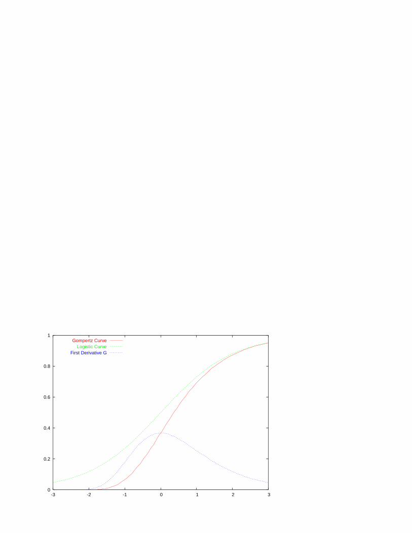
0
0.2
0.4
0.6
0.8
1
-3 -2 -1 0 1 2 3
Gompertz CurveLogistic Curve
First Derivative G
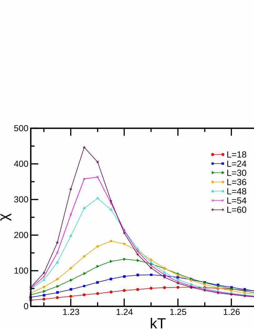
1.23 1.24 1.25 1.26
kT0
100
200
300
400
500
χ
L=18L=24L=30L=36L=48L=54L=60
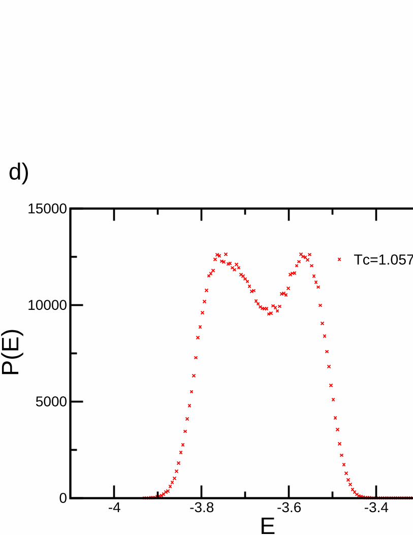
-4 -3.8 -3.6 -3.4
E0
5000
10000
15000
P(E
)
Tc=1.05758
d)
Related Documents