MS1b Statistical Data Mining Part 2: Supervised Learning ...teh/teaching/datamining/part2.pdf · Outline Supervised Learning: Parametric Methods Decision Theory Linear Discriminant

MS1b Statistical Data MiningPart 2: Supervised Learning

Parametric Methods

Yee Whye TehDepartment of Statistics

Oxford

http://www.stats.ox.ac.uk/~teh/datamining.html

http://www.stats.ox.ac.uk/~teh/datamining.html

Outline

Supervised Learning: Parametric MethodsDecision TheoryLinear Discriminant AnalysisQuadratic Discriminant AnalysisNaïve BayesBayesian MethodsLogistic RegressionEvaluating Learning Methods

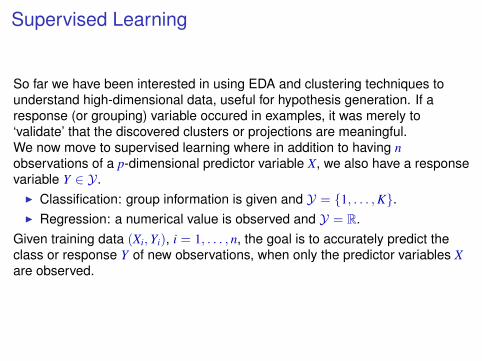
Supervised Learning

So far we have been interested in using EDA and clustering techniques tounderstand high-dimensional data, useful for hypothesis generation. If aresponse (or grouping) variable occured in examples, it was merely to‘validate’ that the discovered clusters or projections are meaningful.We now move to supervised learning where in addition to having nobservations of a p-dimensional predictor variable X, we also have a responsevariable Y ∈ Y.

I Classification: group information is given and Y = {1, . . . ,K}.I Regression: a numerical value is observed and Y = R.

Given training data (Xi,Yi), i = 1, . . . , n, the goal is to accurately predict theclass or response Y of new observations, when only the predictor variables Xare observed.

Outline


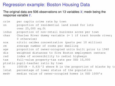
Regression example: Boston Housing DataThe original data are 506 observations on 13 variables X; medv being theresponse variable Y.

crim per capita crime rate by townzn proportion of residential land zoned for lots

over 25,000 sq.ftindus proportion of non-retail business acres per townchas Charles River dummy variable (= 1 if tract bounds river;

0 otherwise)nox nitric oxides concentration (parts per 10 million)rm average number of rooms per dwellingage proportion of owner-occupied units built prior to 1940dis weighted distances to five Boston employment centersrad index of accessibility to radial highwaystax full-value property-tax rate per USD 10,000ptratio pupil-teacher ratio by townb 1000(B - 0.63)^2 where B is the proportion of blacks by townlstat percentage of lower status of the populationmedv median value of owner-occupied homes in USD 1000’s

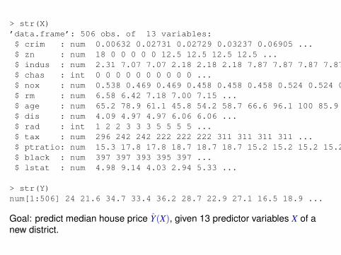
> str(X)’data.frame’: 506 obs. of 13 variables:$ crim : num 0.00632 0.02731 0.02729 0.03237 0.06905 ...$ zn : num 18 0 0 0 0 0 12.5 12.5 12.5 12.5 ...$ indus : num 2.31 7.07 7.07 2.18 2.18 2.18 7.87 7.87 7.87 7.87 ...$ chas : int 0 0 0 0 0 0 0 0 0 0 ...$ nox : num 0.538 0.469 0.469 0.458 0.458 0.458 0.524 0.524 0.524 0.524 ...$ rm : num 6.58 6.42 7.18 7.00 7.15 ...$ age : num 65.2 78.9 61.1 45.8 54.2 58.7 66.6 96.1 100 85.9 ...$ dis : num 4.09 4.97 4.97 6.06 6.06 ...$ rad : int 1 2 2 3 3 3 5 5 5 5 ...$ tax : num 296 242 242 222 222 222 311 311 311 311 ...$ ptratio: num 15.3 17.8 17.8 18.7 18.7 18.7 15.2 15.2 15.2 15.2 ...$ black : num 397 397 393 395 397 ...$ lstat : num 4.98 9.14 4.03 2.94 5.33 ...

> str(Y)num[1:506] 24 21.6 34.7 33.4 36.2 28.7 22.9 27.1 16.5 18.9 ...

Goal: predict median house price Y(X), given 13 predictor variables X of anew district.

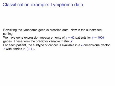
Classification example: Lymphoma data

Revisiting the lymphoma gene expression data. Now in the supervisedsetting.We have gene expression measurements of n = 62 patients for p = 4026genes. These form the predictor variable matrix X.For each patient, the subtype of cancer is available in a n dimensional vectorY with entries in {0, 1}.

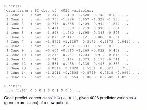
> str(X)’data.frame’: 62 obs. of 4026 variables:$ Gene 1 : num -0.344 -1.188 0.520 -0.748 -0.868 ...$ Gene 2 : num -0.953 -1.286 0.657 -1.328 -1.330 ...$ Gene 3 : num -0.776 -0.588 0.409 -0.991 -1.517 ...$ Gene 4 : num -0.474 -1.588 0.219 0.978 -1.604 ...$ Gene 5 : num -1.896 -1.960 -1.695 -0.348 -0.595 ...$ Gene 6 : num -2.075 -2.117 0.121 -0.800 0.651 ...$ Gene 7 : num -1.8755 -1.8187 0.3175 0.3873 0.0414 ...$ Gene 8 : num -1.539 -2.433 -0.337 -0.522 -0.668 ...$ Gene 9 : num -0.604 -0.710 -1.269 -0.832 0.458 ...$ Gene 10 : num -0.218 -0.487 -1.203 -0.919 -0.848 ...$ Gene 11 : num -0.340 1.164 1.023 1.133 -0.541 ...$ Gene 12 : num -0.531 0.488 -0.335 0.496 -0.358 ...$ Gene 13 : num 0.0846 0.4820 1.5254 0.0323 -0.7563 ...$ Gene 14 : num -1.2011 -0.0505 -0.8799 0.7518 -0.9964 ...$ Gene 15 : num -0.9588 -0.0554 -1.0008 0.2502 -1.0235 ...

> str(Y)num [1:62] 0 0 0 1 0 0 1 0 0 0 ...

Goal: predict ‘cancer class’ Y(X) ∈ {0, 1}, given 4026 predictor variables X(gene expressions) of a new patient.

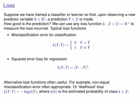
LossSuppose we have trained a classifier or learner so that, upon observing a newpredictor variable X ∈ Rp, a prediction Y ∈ Y is made.How good is the prediction? We can use any loss function L : Y × Y 7→ R+ tomeasure the loss incurred. Typical loss functions

I Misclassification error for classification

L(Y, Y) =

{0 Y = Y1 Y 6= Y

.

I Squared error loss for regression

L(Y, Y) = (Y − Y)2.

Alternative loss functions often useful. For example, non-equalmisclassification error often appropriate. Or ‘likelihood’-lossL(Y, Y) = − log p(Y), where p(k) is the estimated probability of class k ∈ Y.

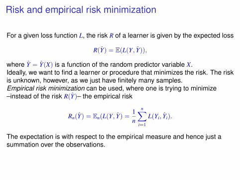
Risk and empirical risk minimization

For a given loss function L, the risk R of a learner is given by the expected loss

R(Y) = E(L(Y, Y)),

where Y = Y(X) is a function of the random predictor variable X.Ideally, we want to find a learner or procedure that minimizes the risk. The riskis unknown, however, as we just have finitely many samples.Empirical risk minimization can be used, where one is trying to minimize–instead of the risk R(Y)– the empirical risk

Rn(Y) = En(L(Y, Y) =1n

n∑

i=1

L(Yi, Yi).

The expectation is with respect to the empirical measure and hence just asummation over the observations.

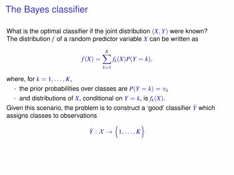
The Bayes classifier

What is the optimal classifier if the joint distribution (X,Y) were known?The distribution f of a random predictor variable X can be written as

f (X) =

K∑

k=1

fk(X)P(Y = k),

where, for k = 1, . . . ,K,- the prior probabilities over classes are P(Y = k) = πk

- and distributions of X, conditional on Y = k, is fk(X).Given this scenario, the problem is to construct a ‘good’ classifier Y whichassigns classes to observations

Y : X →{

1, . . . ,K}

We are interested in finding the classifier Y that minimises the risk under 0-1loss, the Bayes Classifier.

R(Y) = E[L(Y, Y(X))

]

= E[E[L(Y, Y(x)

∣∣X = x]]

=

∫

XE[L(Y, Y(x))

∣∣X = x]f (x)dx

For the Bayes classifier, minimizing E[L(Y, Y(x))

∣∣X = x]

for each x suffices.

That is, given X = x, want to choose Y(x) ∈ {1, . . . ,K} such that the expectedconditional loss is as small as possible.

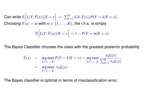
Can write E[L(Y, Y(x))

∣∣X = x]

=∑K

k=1 L(k, Y(x))P(Y = k|X = x).

Choosing Y(x) = m with m ∈ {1, . . . ,K}, the r.h.s. is simply

E[L(Y, Y(x))|X = x

]= 1− P(Y = m|X = x).

The Bayes Classifier chooses the class with the greatest posterior probability

Y(x) = arg maxk=1,...,K

P(Y = k|X = x) = arg maxk=1,...,K

πkfk(x)∑Kk=1 πkfk(x)

= arg maxk=1,...,K

πkfk(x).

The Bayes classifier is optimal in terms of misclassification error.

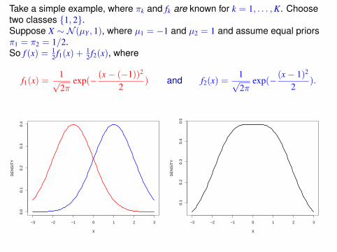
Take a simple example, where πk and fk are known for k = 1, . . . ,K. Choosetwo classes {1, 2}.Suppose X ∼ N (µY , 1), where µ1 = −1 and µ2 = 1 and assume equal priorsπ1 = π2 = 1/2.So f (x) = 1

2 f1(x) + 12 f2(x), where

f1(x) =1√2π

exp(− (x− (−1))2

2) and f2(x) =

1√2π

exp(− (x− 1)2

2).

−3 −2 −1 0 1 2 3

0.0

0.1

0.2

0.3

0.4

X

DE

NS

ITY

−3 −2 −1 0 1 2 3

0.1

0.2

0.3

0.4

0.5

X

DE

NS

ITY

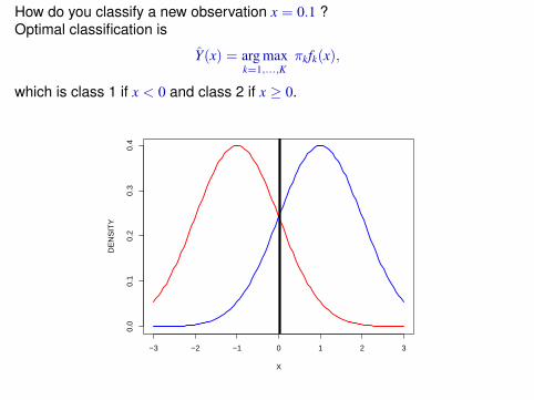
How do you classify a new observation x = 0.1 ?Optimal classification is


πkfk(x),

which is class 1 if x < 0 and class 2 if x ≥ 0.

−3 −2 −1 0 1 2 3

0.0

0.1

0.2

0.3

0.4

X

DE

NS

ITY

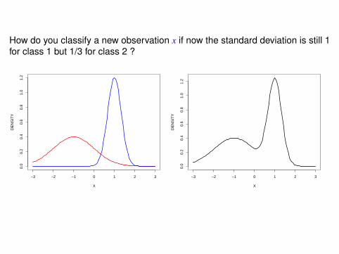
How do you classify a new observation x if now the standard deviation is still 1for class 1 but 1/3 for class 2 ?

−3 −2 −1 0 1 2 3

0.0

0.2

0.4

0.6

0.8

1.0

1.2

X

DE

NS

ITY

−3 −2 −1 0 1 2 30.

00.

20.

40.

60.

81.

01.

2X

DE

NS

ITY

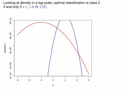
Looking at density in a log-scale, optimal classification is class 2if and only if x ∈ [−0.39, 2.15].

−3 −2 −1 0 1 2 3

1e−

045e

−04

5e−

035e

−02

5e−

01

X

DE

NS

ITY

Plug-in classification

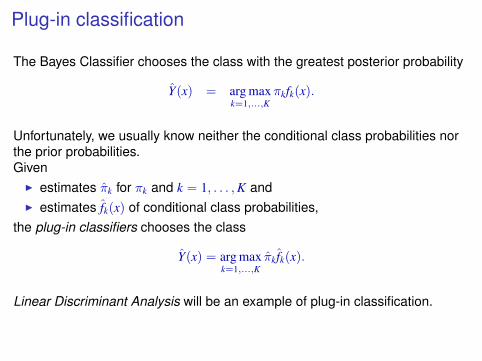
The Bayes Classifier chooses the class with the greatest posterior probability


πkfk(x).

Unfortunately, we usually know neither the conditional class probabilities northe prior probabilities.Given

I estimates πk for πk and k = 1, . . . ,K andI estimates fk(x) of conditional class probabilities,

the plug-in classifiers chooses the class


πk fk(x).

Linear Discriminant Analysis will be an example of plug-in classification.

Outline


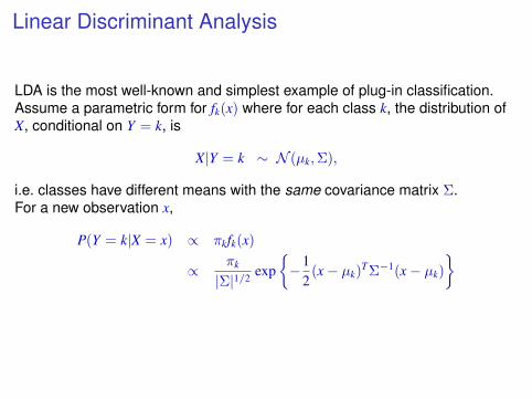
Linear Discriminant Analysis

LDA is the most well-known and simplest example of plug-in classification.Assume a parametric form for fk(x) where for each class k, the distribution ofX, conditional on Y = k, is

X|Y = k ∼ N (µk,Σ),

i.e. classes have different means with the same covariance matrix Σ.For a new observation x,

P(Y = k|X = x) ∝ πkfk(x)

∝ πk

|Σ|1/2 exp{−1

2(x− µk)

TΣ−1(x− µk)

}

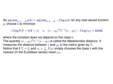
As arg maxk=1,...,K g(k) = arg mink=1,...,K −2 log g(k) for any real-valued functiong, choose k to minimize

−2 log P(Y = k|X = x) ∝ (x− µk)TΣ−1(x− µk)− 2 log(πk) + const.

where the constant does not depend on the class k.The quantity (x− µk)

TΣ−1(x− µk) is called the Malahanobis distance. Itmeasures the distance between x and µk in the metric given by Σ.Notice that if Σ = Ip and πk = 1

K , Y(x) simply chooses the class k with thenearest (in the Euclidean sense) mean µk.

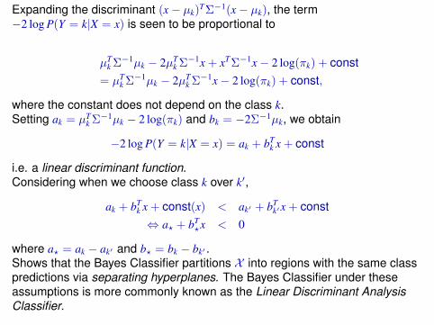
Expanding the discriminant (x− µk)TΣ−1(x− µk), the term

−2 log P(Y = k|X = x) is seen to be proportional to

µTk Σ−1µk − 2µT

k Σ−1x + xTΣ−1x− 2 log(πk) + const= µT

k Σ−1µk − 2µTk Σ−1x− 2 log(πk) + const,

where the constant does not depend on the class k.Setting ak = µT

k Σ−1µk − 2 log(πk) and bk = −2Σ−1µk, we obtain

−2 log P(Y = k|X = x) = ak + bTk x + const

i.e. a linear discriminant function.Considering when we choose class k over k′,

ak + bTk x + const(x) < ak′ + bT

k′x + const⇔ a? + bT

?x < 0

where a? = ak − ak′ and b? = bk − bk′ .Shows that the Bayes Classifier partitions X into regions with the same classpredictions via separating hyperplanes. The Bayes Classifier under theseassumptions is more commonly known as the Linear Discriminant AnalysisClassifier.

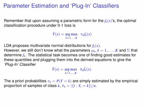
Parameter Estimation and ‘Plug-In’ Classifiers

Remember that upon assuming a parametric form for the fk(x)’s, the optimalclassification procedure under 0-1 loss is


πkfk(x)

LDA proposes multivariate normal distributions for fk(x).However, we still don’t know what the parameters µk, k = 1, . . . ,K and Σ thatdetermine fk. The statistical task becomes one of finding good estimates forthese quantities and plugging them into the derived equations to give the‘Plug-In’ Classifier


πk fk(x).

The a priori probabilities πk = P(Y = k) are simply estimated by the empiricalproportion of samples of class k, πk = |{i : Yi = k}|/n.

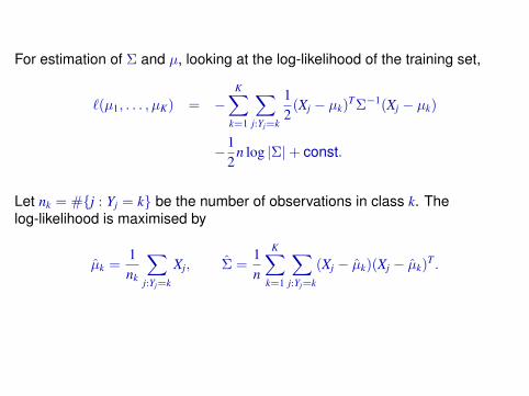
For estimation of Σ and µ, looking at the log-likelihood of the training set,

`(µ1, . . . , µK) = −K∑

k=1

∑

j:Yj=k

12

(Xj − µk)TΣ−1(Xj − µk)

−12

n log |Σ|+ const.

Let nk = #{j : Yj = k} be the number of observations in class k. Thelog-likelihood is maximised by

µk =1nk

∑

j:Yj=k

Xj, Σ =1n

K∑

k=1

∑

j:Yj=k

(Xj − µk)(Xj − µk)T .

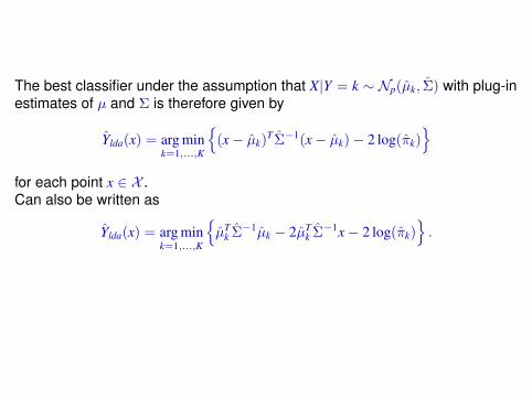
The best classifier under the assumption that X|Y = k ∼ Np(µk, Σ) with plug-inestimates of µ and Σ is therefore given by

Ylda(x) = arg mink=1,...,K

{(x− µk)

TΣ−1(x− µk)− 2 log(πk)}

for each point x ∈ X .Can also be written as

Ylda(x) = arg mink=1,...,K

{µT

k Σ−1µk − 2µTk Σ−1x− 2 log(πk)

}.

Iris example

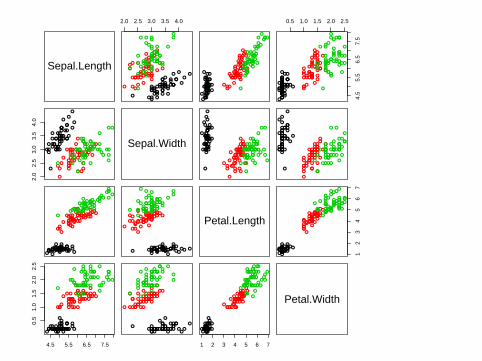
library(MASS)data(iris)

##save class labelsct <- rep(1:3,each=50)##pairwise plotpairs(iris[,1:4],col=ct)

##save petal.length and petal.widthiris.data <- iris[,3:4]plot(iris.data,col=ct+1,pch=20,cex=1.5,cex.lab=1.4)

Sepal.Length

2.0 2.5 3.0 3.5 4.0

●●

●●

●

●

●

●

●

●

●

●●

●

●●

●

●

●

●

●

●

●

●

●● ●

●●

●●

●●

●

●●

●

●

●

●●

●●

●●

●

●

●

●

●

●

●

●

●

●

●

●

●

●

●●

●●

●

●

●

●●

●

●

●●

●●

●●

●●

●

●●●

●●

●

●

●

●

●●●

●

●

●

●●●

●

●

●

●

●

●

●●

●

●

●

●

●

●●

●

●●

●●

●●

●

●

●

●

●

●

●

●●

●

●●

●

●●

●

●

●●

●

●●●

●

●●●

●●

●

●

●●

●●

●

●

●

●

●

●

●

●●

●

●●

●

●

●

●

●

●

●

●

●●●

●●

●●

●●

●

●●

●

●

●

●●

●●

●●

●

●

●

●

●

●

●

●

●

●

●

●

●

●

●●

●●

●

●

●

●●

●

●

●●

●●

●●

●●

●

●●●

●●

●

●

●

●

●● ●

●

●

●

●●●

●

●

●

●

●

●

●●

●

●

●

●

●

●●

●

●●

●●

●●

●

●

●

●

●

●

●

●●

●

●●

●

●●

●

●

●●

●

●●

●

●

●●●

●●

●

●

0.5 1.0 1.5 2.0 2.5

4.5

5.5

6.5

7.5

●●●●

●

●

●

●

●

●

●

●●

●

●●

●

●

●

●

●

●

●

●

●● ●●●

●●

●●

●

●●

●

●

●

●●

●●

●●

●

●

●

●

●

●

●

●

●

●

●

●

●

●

●●

●●

●

●

●

●●

●

●

●●

●●

●●●

●

●

●●●

●●

●

●

●

●

●●●

●

●

●

●●●

●

●

●

●

●

●

●●

●

●

●

●

●

●●

●

●●

●●

●●

●

●

●

●

●

●

●

●●

●

●●

●

●●

●

●

●●

●

●●

●

●

●●●

●●

●

●

2.0

2.5

3.0

3.5

4.0

●

●

●●

●

●

● ●

●

●

●

●

●●

●

●

●

●

●●

●

●●

●●

●

●●●

●●

●

●●

●●

●●

●

●●

●

●

●

●

●

●

●

●

●●●

●

●

●●

●

●

●

●

●

●

●

●●

●●

●

●

●

●

●

●

●●

●

●

●●

●

●●

● ●

●

●

●

●

●

●●

●

●

●

●

●● ●

●

●

●

●

●●

● ●

●

●

●

●

●

●

●

●

●

●

●

●

●

●

●

● ●●

●●

●

●

●

●

●

●

●●

●

●

●

●●

●● ●

●

●●

●

●

●

●

●Sepal.Width

●

●

●●

●

●

●●

●

●

●

●

●●

●

●

●

●

●●

●

●●

●●

●

●●

●

●●

●

●●

●●

●●

●

●●

●

●

●

●

●

●

●

●

●●●

●

●

●●

●

●

●

●

●

●

●

●●

●●

●

●

●

●

●

●

●●●

●

●●

●

●●

● ●

●

●

●

●

●

●●

●

●

●

●

●●●

●

●

●

●

●●

● ●

●

●

●

●

●

●

●

●

●

●

●

●

●

●

●

● ●●

●●

●

●

●

●

●

●

●●

●

●

●

●●

●●●

●

●●

●

●

●

●

●

●

●

●●

●

●

●●

●

●

●

●

●●

●

●

●

●

●●

●

●●

●●

●

●●●

●●

●

●●

●●

●●

●

●●

●

●

●

●

●

●

●

●

●●●

●

●

●●

●

●

●

●

●

●

●

●●

●●

●

●

●

●

●

●

●●

●

●

●●

●

●●

● ●

●

●

●

●

●

●●

●

●

●

●

●●●

●

●

●

●

●●

●●

●

●

●

●

●

●

●

●

●

●

●

●

●

●

●

●●●

●●

●

●

●

●

●

●

●●

●

●

●

●●

● ●●

●

●●

●

●

●

●

●

●●●● ●

●● ●● ● ●●

●● ●

●●●

●●

●●

●

●●

●● ●●●● ●● ●●

● ●●●●

●●●●●

●●

● ●●

●●

●

●

●●●

●

●

●

●

●●

●

●

●●

●

●

●

●

●

●●

● ●

●●

●

●●●

●

●

● ●●

●●●

●●

●

●

●●● ●

●

●

●

●

●●

●

●

●

●

●●

●●

●

●●●●

●●

●

●

●

●

●

●●

●●

●●

●●

●

●

●

●

●●

●

●●

●●

●●

●●

●●

●

●● ●● ●

●●●● ● ●●

●● ●

●●●

●●

●●

●

●●

● ●●●●● ● ●●●● ●●●

●●● ●●

●

●●

● ●●

●●

●

●

●●●

●

●

●

●

●●

●

●

●●

●

●

●

●

●

●●

●●

●●

●

●●●

●

●

● ●●

●●●

●●

●

●

● ●●●

●

●

●

●

●●

●

●

●

●

●●

●●

●

● ●●

●

●●

●

●

●

●

●

●●

● ●

●●

●●

●

●

●

●

●●

●

●●

●●

●●

●●

●●

●

Petal.Length

12

34

56

7

●●●●●

●●●●●●●●

●●●●●

●●

●●

●

●●● ●●●●● ●●●●●●

●●●

●●●●

●

●●●●●

●●

●

●

●●●

●

●

●

●

●●

●

●

●●

●

●

●

●

●

●●

●●

●●

●

●●●

●

●

●●●

●●●

●●

●

●

●●●●

●

●

●

●

●●

●

●

●

●

●●

●●

●

● ●●

●

●●

●

●

●

●

●

●●

●●

●●

●●

●

●

●

●

●●

●

●●

●●

●●

●●

●●

●

4.5 5.5 6.5 7.5

0.5

1.0

1.5

2.0

2.5

●●●● ●

●●

●●●

●●●●

●

●●● ●●

●

●

●

●

● ●

●

●●●●

●

●●●● ●

●● ●

●●●

●

●●

●● ●●

●● ●

●

●

●

●

●

●●

●

●

●

●●

●●

●

●

●

●

●

●

●●

● ●

●

●

●●●

●

●●

●●

●●●●

●

●

●

●●● ●

●

●

●

●

●

●

●●

●●●

●

●●

●●

●●

●

●●

●

●

● ●

●

●

●●●

●

●

●●

●

●●

●●

●●

●

●●

●

●

●

●

●●

●

●

●● ●● ●

●●●●

●●●

●●●

●●● ●●

●

●

●

●

●●

●

●●●●

●

●●●● ●

●● ●

●●●

●

●●

●● ●●

●●●

●

●

●

●

●

●●

●

●

●

●●

●●

●

●

●

●

●

●

●●

●●

●

●

●●●

●

●●

●●

● ●●●

●

●

●

●●

●●

●

●

●

●

●

●

●●

●●●

●

●●

●●

●●

●

●●

●

●

●●

●

●

●● ●

●

●

●●

●

●●

●●

●●

●

●●

●

●

●

●

●●

●

●

1 2 3 4 5 6 7

●●●●●

●●●●●●●

●●●

●●●●●

●

●

●

●

●●

●

●●●●

●

●●●●●●

●●●●●

●

●●

●●●●

●● ●

●

●

●

●

●

●●

●

●

●

●●

●●

●

●

●

●

●

●

●●● ●

●

●

●●

●

●

●●●

●

●●●●

●

●

●

●●●●

●

●

●

●

●

●

●●

●●●

●

●●

●●

●●

●

●●

●

●

● ●

●

●

●●●

●

●

●●

●

●●

●●

●●

●

●●

●

●

●

●

●●

●

●

Petal.Width

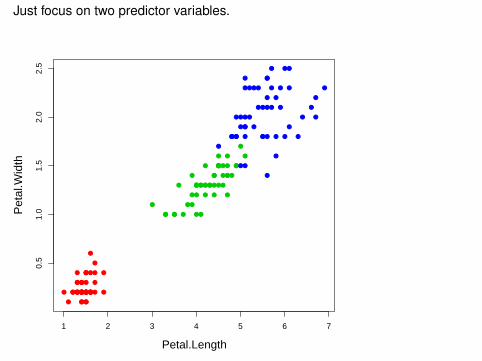
Just focus on two predictor variables.

●●● ●●

●

●

●●

●

●●

●●

●

●●

● ●●

●

●

●

●

●●

●

●● ●●

●

●

●●●●

●

● ●

●●

●

●

●

●

●●●●

●

● ●

●

●

●

●

●

●

●

●

●

●

●

●

●

●

●

●

●

●

●

●

●

●

● ●

●

●

●

●

●

●

●

●

●

●

●●●

●

●

●

●

●

●

●●

●

●

●

●

●

●

●

●

●

●●

●

●

●

●

●

●

●

●

●

●

●

●

● ●

●

●

●●●

●

●

●

●

●

●

●

●

●

●●

●

●

●

●

●

●

●

●

●

●

●

1 2 3 4 5 6 7

0.5

1.0

1.5

2.0

2.5

Petal.Length

Pet

al.W

idth

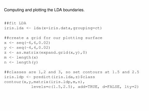
Computing and plotting the LDA boundaries.

##fit LDAiris.lda <- lda(x=iris.data,grouping=ct)

##create a grid for our plotting surfacex <- seq(-6,6,0.02)y <- seq(-4,4,0.02)z <- as.matrix(expand.grid(x,y),0)m <- length(x)n <- length(y)

##classes are 1,2 and 3, so set contours at 1.5 and 2.5iris.ldp <- predict(iris.lda,z)$classcontour(x,y,matrix(iris.ldp,m,n),

levels=c(1.5,2.5), add=TRUE, d=FALSE, lty=2)

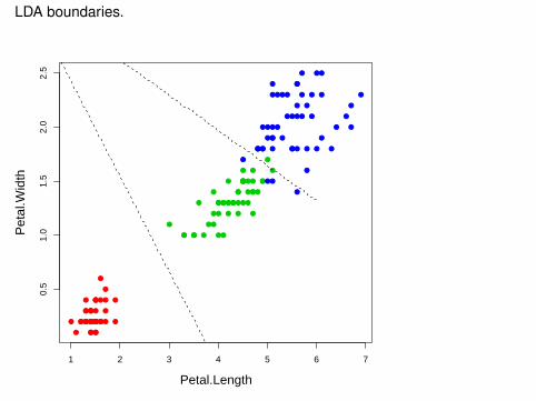
LDA boundaries.

●●● ●●

●

●

●●

●

●●

●●

●

●●

● ●●

●

●

●

●

●●

●

●● ●●

●

●

●●●●

●

● ●

●●

●

●

●

●

●●●●

●

● ●

●

●

●

●

●

●

●

●

●

●

●

●

●

●

●

●

●

●

●

●

●

●

● ●

●

●

●

●

●

●

●

●

●

●

●●●

●

●

●

●

●

●

●●

●

●

●

●

●

●

●

●

●

●●

●

●

●

●

●

●

●

●

●

●

●

●

● ●

●

●

●●●

●

●

●

●

●

●

●

●

●

●●

●

●

●

●

●

●

●

●

●

●

●

1 2 3 4 5 6 7

0.5

1.0

1.5

2.0

2.5

Petal.Length

Pet

al.W

idth

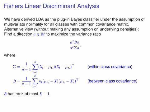
Fishers Linear Discriminant Analysis

We have derived LDA as the plug-in Bayes classifier under the assumption ofmultivariate normality for all classes with common covariance matrix.Alternative view (without making any assumption on underlying densities):Find a direction a ∈ Rp to maximize the variance ratio

aTBaaTΣa

,

where

Σ =1

n− 1

n∑

i=1

(Xi − µYi)(Xi − µYi)> (within class covariance)

B =1

n− 1

K∑

k=1

nk(µYi − X)(µYi − X))> (between class covariance)

B has rank at most K − 1.

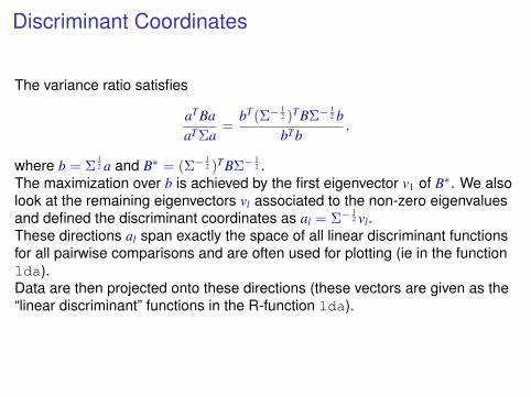
Discriminant Coordinates

The variance ratio satisfies

aTBaaTΣa

=bT(Σ−

12 )TBΣ−

12 b

bTb,

where b = Σ12 a and B∗ = (Σ−

12 )TBΣ−

12 .

The maximization over b is achieved by the first eigenvector v1 of B∗. We alsolook at the remaining eigenvectors vl associated to the non-zero eigenvaluesand defined the discriminant coordinates as al = Σ−

12 vl.

These directions al span exactly the space of all linear discriminant functionsfor all pairwise comparisons and are often used for plotting (ie in the functionlda).Data are then projected onto these directions (these vectors are given as the“linear discriminant” functions in the R-function lda).

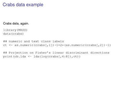
Crabs data example

Crabs data, again.

library(MASS)data(crabs)

## numeric and text class labelsct <- as.numeric(crabs[,1])-1+2*(as.numeric(crabs[,2])-1)

## Projection on Fisher’s linear discriminant directionsprint(cb.lda <- lda(log(crabs[,4:8]),ct))

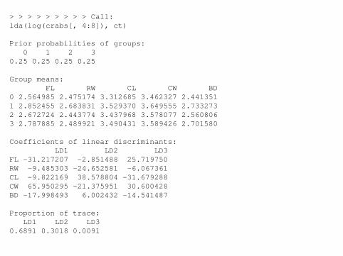
> > > > > > > > > Call:lda(log(crabs[, 4:8]), ct)

Prior probabilities of groups:0 1 2 3

0.25 0.25 0.25 0.25

Group means:FL RW CL CW BD

0 2.564985 2.475174 3.312685 3.462327 2.4413511 2.852455 2.683831 3.529370 3.649555 2.7332732 2.672724 2.443774 3.437968 3.578077 2.5608063 2.787885 2.489921 3.490431 3.589426 2.701580

Coefficients of linear discriminants:LD1 LD2 LD3

FL -31.217207 -2.851488 25.719750RW -9.485303 -24.652581 -6.067361CL -9.822169 38.578804 -31.679288CW 65.950295 -21.375951 30.600428BD -17.998493 6.002432 -14.541487

Proportion of trace:LD1 LD2 LD3

0.6891 0.3018 0.0091

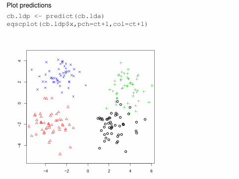
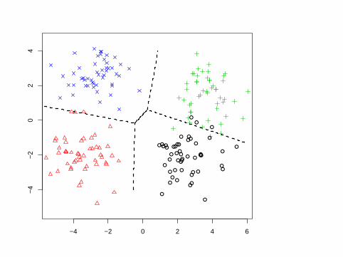
Plot predictions

cb.ldp <- predict(cb.lda)eqscplot(cb.ldp$x,pch=ct+1,col=ct+1)

●

●

●

●

●

●

●●

●

●

●●

●

●

●

●

●●

●

●

●

●

●

●

●

●

●

●

●

●

●

●

●

●

●

●

●

●

●●

●

●

●

●

●

●

●

●

●

●

−4 −2 0 2 4 6

−4

−2

02

4

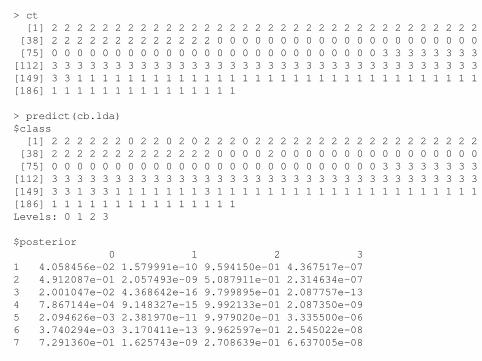
> ct[1] 2 2 2 2 2 2 2 2 2 2 2 2 2 2 2 2 2 2 2 2 2 2 2 2 2 2 2 2 2 2 2 2 2 2 2 2 2[38] 2 2 2 2 2 2 2 2 2 2 2 2 2 0 0 0 0 0 0 0 0 0 0 0 0 0 0 0 0 0 0 0 0 0 0 0 0[75] 0 0 0 0 0 0 0 0 0 0 0 0 0 0 0 0 0 0 0 0 0 0 0 0 0 0 3 3 3 3 3 3 3 3 3 3 3[112] 3 3 3 3 3 3 3 3 3 3 3 3 3 3 3 3 3 3 3 3 3 3 3 3 3 3 3 3 3 3 3 3 3 3 3 3 3[149] 3 3 1 1 1 1 1 1 1 1 1 1 1 1 1 1 1 1 1 1 1 1 1 1 1 1 1 1 1 1 1 1 1 1 1 1 1[186] 1 1 1 1 1 1 1 1 1 1 1 1 1 1 1

> predict(cb.lda)$class[1] 2 2 2 2 2 2 0 2 2 0 2 0 2 2 2 0 2 2 2 2 2 2 2 2 2 2 2 2 2 2 2 2 2 2 2 2 2[38] 2 2 2 2 2 2 2 2 2 2 2 2 2 0 0 0 0 2 0 0 0 0 0 0 0 0 0 0 0 0 0 0 0 0 0 0 0[75] 0 0 0 0 0 0 0 0 0 0 0 0 0 0 0 0 0 0 0 0 0 0 0 0 0 0 3 3 3 3 3 3 3 3 3 3 3[112] 3 3 3 3 3 3 3 3 3 3 3 3 3 3 3 3 3 3 3 3 3 3 3 3 3 3 3 3 3 3 3 3 3 3 3 3 3[149] 3 3 1 3 3 1 1 1 1 1 1 1 3 1 1 1 1 1 1 1 1 1 1 1 1 1 1 1 1 1 1 1 1 1 1 1 1[186] 1 1 1 1 1 1 1 1 1 1 1 1 1 1 1Levels: 0 1 2 3

$posterior0 1 2 3

1 4.058456e-02 1.579991e-10 9.594150e-01 4.367517e-072 4.912087e-01 2.057493e-09 5.087911e-01 2.314634e-073 2.001047e-02 4.368642e-16 9.799895e-01 2.087757e-134 7.867144e-04 9.148327e-15 9.992133e-01 2.087350e-095 2.094626e-03 2.381970e-11 9.979020e-01 3.335500e-066 3.740294e-03 3.170411e-13 9.962597e-01 2.545022e-087 7.291360e-01 1.625743e-09 2.708639e-01 6.637005e-08

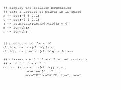
## display the decision boundaries## take a lattice of points in LD-spacex <- seq(-6,6,0.02)y <- seq(-4,4,0.02)z <- as.matrix(expand.grid(x,y,0))m <- length(x)n <- length(y)

## predict onto the gridcb.ldap <- lda(cb.ldp$x,ct)cb.ldpp <- predict(cb.ldap,z)$class

## classes are 0,1,2 and 3 so set contours## at 0.5,1.5 and 2.5contour(x,y,matrix(cb.ldpp,m,n),

levels=c(0.5,2.5),add=TRUE,d=FALSE,lty=2,lwd=2)

●

●

●

●

●

●

●●

●

●

●●

●

●

●

●

●●

●

●

●

●

●

●

●

●

●

●

●

●

●

●

●

●

●

●

●

●

●●

●

●

●

●

●

●

●

●

●

●

−4 −2 0 2 4 6

−4

−2

02

4

Compare with PCA plots.

library(lattice)cb.pca <- princomp(log(crabs[,4:8]))cb.pcp <- predict(cb.pca)splom(~cb.pcp[,1:3],pch=ct+1,col=ct+1)

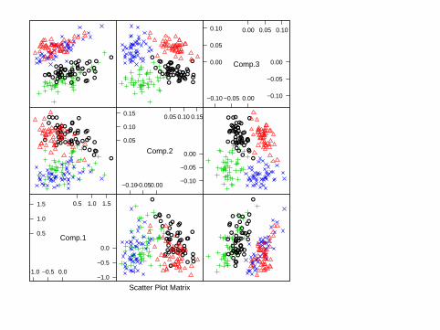
Scatter Plot Matrix

Comp.10.5

1.0

1.5 0.5 1.0 1.5

−1.0

−0.5

0.0

−1.0 −0.5 0.0

●

●●●●● ●● ●● ●

●●● ●●

●●●

●● ●●●● ●● ●●● ●● ●●● ●● ●●

● ●●●

● ●●●●●

●

●

● ●●●●● ●●

●●●

● ● ●●●

●●● ●●●●● ●●●●●●

●●●●●●●●

●●●●

●● ●●

●●●

●

●

●●●

●

●●

●

●

●

●

●●

●

●

●

●●

●

●

●

●

●●

●

●

●●

●

●

●●

●●

●

●

●

●●

●

●

●

●

●

●

●●

●

●

Comp.2

0.05

0.10

0.15 0.05 0.10 0.15

−0.10

−0.05

0.00

−0.10−0.050.00

●

●

●●●

●

● ●

●

●

●

●

●●

●

●

●

●●

●

●

●

●

●●

●

●

●●

●

●

●●

●●

●

●

●

●●

●

●

●

●

●

●

●●

●

●

●

●

●

●●

●

●

●

●

●

●

●

●

●

●

●

●

●●

●

●

●

●●

●

●●●

●●

●

●

●●●

●●●●●

●●●

●

●

●

●●●●

●

●

●

●●

●

●

●

●

●

●

●

●

●

●

●

●

●●

●

●

●

●●

●

●● ●

●●

●

●

●●●

●●●

●●

● ●●

●

●

●

●●●●

Comp.30.00

0.05

0.10 0.00 0.05 0.10

−0.10

−0.05

0.00

−0.10 −0.05 0.00

●

●

●

●

●

●

●●

●

●

●●

●

●

●

●

●●

●

●

●

●

●

●

●

●

●

●

●

●

●

●

●

●

●

●

●

●

●●

●

●

●

●

●

●

●

●

●

●

−4 −2 0 2 4 6

−4

−2

02

4

●

●

●

●

●

●

●

●

●

●

●

●

●

●

●

●

●

●●

●

●

●

●●

●

●

● ●

●●

●

●

●

●●

●●

●

●●

●●

●

●

●

●

●

●●●

−0.10 −0.05 0.00 0.05 0.10 0.15

−0.

10−

0.05

0.00

0.05

0.10

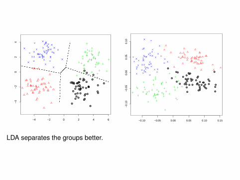
LDA separates the groups better.

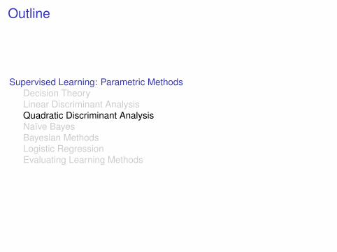
Outline


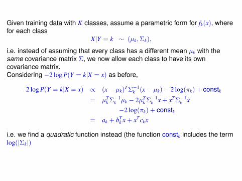
Given training data with K classes, assume a parametric form for fk(x), wherefor each class

X|Y = k ∼ (µk,Σk),

i.e. instead of assuming that every class has a different mean µk with thesame covariance matrix Σ, we now allow each class to have its owncovariance matrix.Considering −2 log P(Y = k|X = x) as before,

−2 log P(Y = k|X = x) ∝ (x− µk)TΣ−1

k (x− µk)− 2 log(πk) + constk= µT

k Σ−1k µk − 2µT

k Σ−1k x + xTΣ−1

k x

−2 log(πk) + constk= ak + bT

k x + xTckx

i.e. we find a quadratic function instead (the function constk includes the termlog(|Σk|)

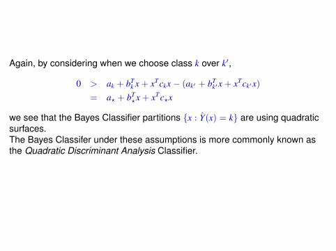
Again, by considering when we choose class k over k′,

0 > ak + bTk x + xTckx− (ak′ + bT

k′x + xTck′x)

= a? + bT?x + xTc?x

we see that the Bayes Classifier partitions {x : Y(x) = k} are using quadraticsurfaces.The Bayes Classifer under these assumptions is more commonly known asthe Quadratic Discriminant Analysis Classifier.

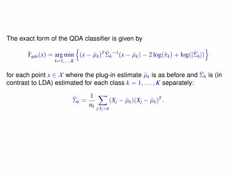
The exact form of the QDA classifier is given by

Yqda(x) = arg mink=1,...,K

{(x− µk)

TΣk−1(x− µk)− 2 log(πk) + log(|Σk|)

}

for each point x ∈ X where the plug-in estimate µk is as before and Σk is (incontrast to LDA) estimated for each class k = 1, . . . ,K separately:

Σk =1nk

∑

j:Yj=k

(Xj − µk)(Xj − µk)T .

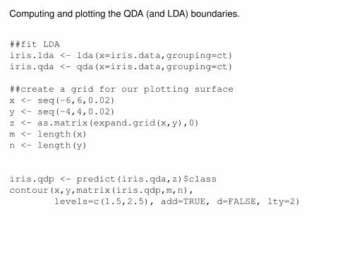
Computing and plotting the QDA (and LDA) boundaries.

##fit LDAiris.lda <- lda(x=iris.data,grouping=ct)iris.qda <- qda(x=iris.data,grouping=ct)

##create a grid for our plotting surfacex <- seq(-6,6,0.02)y <- seq(-4,4,0.02)z <- as.matrix(expand.grid(x,y),0)m <- length(x)n <- length(y)

iris.qdp <- predict(iris.qda,z)$classcontour(x,y,matrix(iris.qdp,m,n),

levels=c(1.5,2.5), add=TRUE, d=FALSE, lty=2)

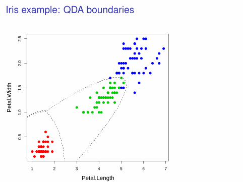
Iris example: QDA boundaries

●●● ●●

●

●

●●

●

●●

●●

●

●●

● ●●

●

●

●

●

●●

●

●● ●●

●

●

●●●●

●

● ●

●●

●

●

●

●

●●●●

●

● ●

●

●

●

●

●

●

●

●

●

●

●

●

●

●

●

●

●

●

●

●

●

●

● ●

●

●

●

●

●

●

●

●

●

●

●●●

●

●

●

●

●

●

●●

●

●

●

●

●

●

●

●

●

●●

●

●

●

●

●

●

●

●

●

●

●

●

● ●

●

●

●●●

●

●

●

●

●

●

●

●

●

●●

●

●

●

●

●

●

●

●

●

●

●

1 2 3 4 5 6 7

0.5

1.0

1.5

2.0

2.5

Petal.Length

Pet

al.W

idth

LDA or QDA?

Having seen both LDA and QDA in action, it is natural to ask which is the“better” classifier.It is obvious that if the covariances of different classes are very distinct, QDAwill probably have an advantage over LDA.As parametric models are only ever approximations to the real world, allowingmore flexible decision boundaries (QDA) may seem like a good idea.However, there is a price to pay in terms of increased variance.

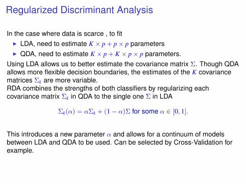
Regularized Discriminant Analysis

In the case where data is scarce , to fitI LDA, need to estimate K × p + p× p parametersI QDA, need to estimate K × p + K × p× p parameters.

Using LDA allows us to better estimate the covariance matrix Σ. Though QDAallows more flexible decision boundaries, the estimates of the K covariancematrices Σk are more variable.RDA combines the strengths of both classifiers by regularizing eachcovariance matrix Σk in QDA to the single one Σ in LDA

Σk(α) = αΣk + (1− α)Σ for some α ∈ [0, 1].

This introduces a new parameter α and allows for a continuum of modelsbetween LDA and QDA to be used. Can be selected by Cross-Validation forexample.

Outline


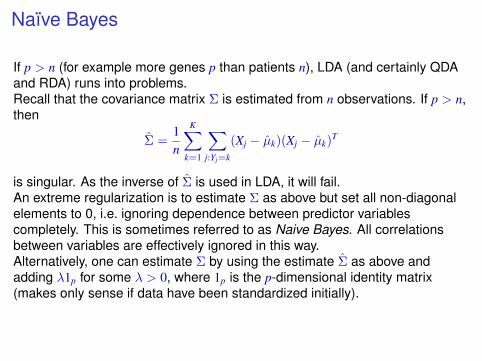
Naïve Bayes

If p > n (for example more genes p than patients n), LDA (and certainly QDAand RDA) runs into problems.Recall that the covariance matrix Σ is estimated from n observations. If p > n,then

Σ =1n

K∑

k=1

∑

j:Yj=k

(Xj − µk)(Xj − µk)T

is singular. As the inverse of Σ is used in LDA, it will fail.An extreme regularization is to estimate Σ as above but set all non-diagonalelements to 0, i.e. ignoring dependence between predictor variablescompletely. This is sometimes referred to as Naive Bayes. All correlationsbetween variables are effectively ignored in this way.Alternatively, one can estimate Σ by using the estimate Σ as above andadding λ1p for some λ > 0, where 1p is the p-dimensional identity matrix(makes only sense if data have been standardized initially).

Applications to Classification of Documents

Given documents such as emails, webpages, scientific articles, books etc., wemight be interested in learning a classifier based on training data toautomatically classify a new document. Possible classes could bespam/non-spam, academic/commercial webpages, maths/physics/biology etc.Many popular techniques rely on simple probabilistic models for documents.Given a prespecified dictionary, we extract high-dimensional features such asabsence/presence of a word (multivariate Bernoulli), number of occurences ofa word (multinomial) etc.Parameters within in class can be estimated through Maximum Likelihood.However Maximum Likelihood overfits so we will need to derive more robustalternative.

Outline


Limitations of Maximum Likelihood

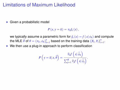
I Given a probabilistic model

P (x, y = k) = πkfk (x) ,

we typically assume a parametric form for fk (x) = f (x|φk) and computethe MLE θ of θ = (πk, φk)

nk=1 based on the training data {Xi,Yi}n

i=1.I We then use a plug-in approach to perform classification

P(

y = k| x, θ)

=πkf(

x| φk

)

∑Kj=1 πjf

(x| φj

) .

Limitations of Maximum Likelihood

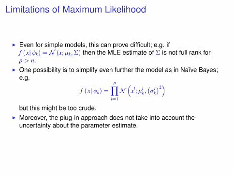
I Even for simple models, this can prove difficult; e.g. iff (x|φk) = N (x;µk,Σ) then the MLE estimate of Σ is not full rank forp > n.

I One possibility is to simplify even further the model as in Naïve Bayes;e.g.

f (x|φk) =

p∏

l=1

N(

xl;µlk,(σl

k

)2)

but this might be too crude.I Moreover, the plug-in approach does not take into account the

uncertainty about the parameter estimate.

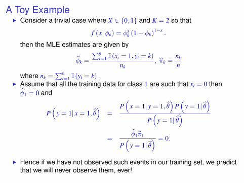
A Toy ExampleI Consider a trivial case where X ∈ {0, 1} and K = 2 so that

f (x|φk) = φxk (1− φk)

1−x.

then the MLE estimates are given by

φk =

∑ni=1 I (xi = 1, yi = k)

nk, πk =

nk

n

where nk =∑n

i=1 I (yi = k) .I Assume that all the training data for class 1 are such that xi = 0 thenφ1 = 0 and

P(

y = 1| x = 1, θ)

=P(

x = 1| y = 1, θ)

P(

y = 1| θ)

P(

y = 1| θ)

=φ1π1

P(

y = 1| θ) = 0.

I Hence if we have not observed such events in our training set, we predictthat we will never observe them, ever!

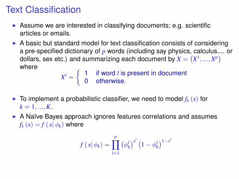
Text ClassificationI Assume we are interested in classifying documents; e.g. scientific

articles or emails.I A basic but standard model for text classification consists of considering

a pre-specified dictionary of p words (including say physics, calculus.... ordollars, sex etc.) and summarizing each document by X =

(X1, ...,Xp

)

where

Xl =

{1 if word l is present in document0 otherwise.

I To implement a probabilistic classifier, we need to model fk (x) fork = 1, ...,K.

I A Naïve Bayes approach ignores features correlations and assumesfk (x) = f (x|φk) where

f (x|φk) =

p∏

l=1

(φl

k

)xl (1− φl

k

)1−xl

Maximum Likelihood for Text Classification

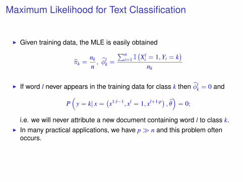
I Given training data, the MLE is easily obtained

πk =nk

n, φl

k =

∑ni=1 I

(Xl

i = 1,Yi = k)

nk

I If word l never appears in the training data for class k then φlk = 0 and

P(

y = k| x =(x1:l−1, xl = 1, xl+1:p) , θ

)= 0;

i.e. we will never attribute a new document containing word l to class k.I In many practical applications, we have p� n and this problem often

occurs.

A Bayesian Approach

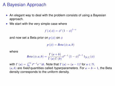
I An elegant way to deal with the problem consists of using a Bayesianapproach.

I We start with the very simple case where

f (x|φ) = φx (1− φ)1−x

and now set a Beta prior on p (φ) on φ

p (φ) = Beta (φ; a, b)

whereBeta (φ; a, b) =

Γ (a + b)

Γ (a) Γ (b)φa−1 (1− φ)

b−1 1[0,1] (φ)

with Γ (u) =∫∞

0 tu−1e−tdt. Note that Γ (u) = (u− 1)! for u ∈ N.(a, b) are fixed quantities called hyperparameters. For a = b = 1, the Betadensity corresponds to the uniform density.

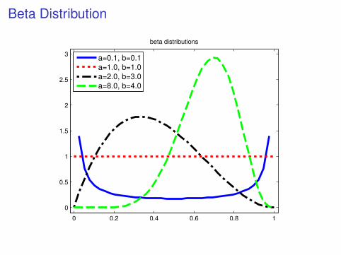
Beta Distribution

0 0.2 0.4 0.6 0.8 1

0

0.5

1

1.5

2

2.5

3

beta distributions

a=0.1, b=0.1

a=1.0, b=1.0

a=2.0, b=3.0

a=8.0, b=4.0

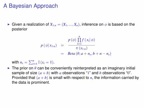
A Bayesian Approach

I Given a realization of X1:n = (X1, ...,Xn), inference on φ is based on theposterior

p (φ| x1:n) =

p (φ)n∏

i=1f (xi|φ)

π (x1:n)

= Beta (θ; a + ns, b + n− ns)

with ns =∑n

i=1 I (xi = 1).I The prior on θ can be conveniently reinterpreted as an imaginary initial

sample of size (a + b) with a observations “1” and b observations “0”.Provided that (a + b) is small with respect to n, the information carried bythe data is prominent.

Beta Posteriors01

02

03

04

05

06

07

08

09

10

11

12

13

14

15

16

17

18

19

20

21

22

23

24

25

26

27

28

29

30

31

32

33

34

35

36

37

38

39

40

41

42

43

44

45

46

47

48

49

50

51

52

53

54

55

56

57

58

59

60

61

bayesBody.tex 127

0 0.1 0.2 0.3 0.4 0.5 0.6 0.7 0.8 0.9 10

1

2

3

4

5

6

prior Be(2.0, 2.0)lik Be(4.0, 18.0)post Be(5.0, 19.0)

(a)

0 0.1 0.2 0.3 0.4 0.5 0.6 0.7 0.8 0.9 10

0.5

1

1.5

2

2.5

3

3.5

4

4.5

prior Be(5.0, 2.0)lik Be(12.0, 14.0)post Be(16.0, 15.0)

(b)

0 0.2 0.4 0.6 0.8 1

0

1

2

3

4

5

6

7

8

9

10

truth

n=5

n=50

n=100

(c)

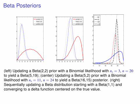
Figure 4.11: (a) Updating a Beta(2,2) prior with a Binomial likelihood with sufficient statistics N1 = 3, N2 = 17 to yield a Beta(5,19)posterior. Figure generated by binomialBetaPosteriorDemo. (b) Updating a Beta(5,2) prior with a Binomial likelihood with sufficientstatistics N1 = 11,N2 = 13 to yield a Beta(16,15) posterior. (c) Sequentially updating a Beta distribution. We start with a Beta(1,1) priorand converge to a delta function centered on the MLE. Figure generated by bernoulliBetaSequentialUpdate.

We see that the posterior has the same functional form (beta) as the prior (beta), since it is conjugate. In particular, the posterioris obtained by adding the prior hyper-parameters αk to the empirical counts Nk. For this reason, the αk hyper-parameters areknown as pseudo counts. The strength of the prior, also known as the effective sample size of the prior, is the sum of thepseudo counts, α1 + α2; this plays a role analogous to the data set size, N1 +N2 = N .

Figure 4.11(a) gives an example where we update a weak Beta(2,2) prior with a peaked likelihood function; we see that theposterior is essentially identical to the likelihood. Figure 4.11(b) gives an example where we update a strong Beta(5,2) priorwith a peaked likelihood function; we see that the posterior is a “compromise” between the prior and likelihood. Compare theseto the analogous pictures for combining a Gaussian prior with a Gaussian likelihood in Figure 5.4.

Figure 4.11(c) shows what happens as the number of samples goes to infinity. Initially (for N = 5), the posterior has askewed shape, but then it becomes more Gaussian-like, and eventually it becomes a delta function centered at the MLE.

Note that updating the posterior sequentially is equivalent to updating in a single batch. To see this, suppose we have twodata sets D1 and D2 with sufficient statistics Na

1 , Na2 and N b

1 , Nb2 . Let N1 = Na

1 + N b1 , N2 = Na

2 + N b2 and N = N1 + N2.

In batch mode we have

p(θ|D1,D2) ∝ Bin(θ|N1, N1 +N2)Beta(θ|α1, α2) ∝ Beta(θ|N1 + α1, N2 + α2) (4.34)

In sequential mode, we have

p(θ|D1,D2) ∝ p(D2|θ)p(θ|D1) (4.35)∝ Bin(θ|N b

1 , Nb1 +N b

2)Beta(θ|Na1 + α1, N

a2 + α2) (4.36)

∝ Beta(θ| Na1 +N b

1 + α1, Na2 +N b

2 + α2) (4.37)

This makes Bayesian inference particularly well-suited to online learning, as we will see later.

4.5.1.4 Posterior mean and mode

It is simple to show that the posterior mode, or MAP estimate, is given by

θMAP =α1 +N1 − 1

α1 + α2 +N − 2(4.38)

By contrast, the posterior mean is given by,

θ =α1 +N1

α1 + α2 +N(4.39)

If we use a uniform prior, αk = 1, then the MAP estimate reduces to the MLE, but the posterior mean estimate does not. Wewill exploit this fact below.

We will now show that the posterior mean is convex combination of the prior mean and the MLE. Let the prior mean bem = (m1,m2), where m1 = α1/α0 and m2 = α2/α0; α0 = α1 + α2 controls the strength of the prior. Then the posteriormean is

E [θ|D] =α0m1 +N1

N + α0=

α0

N + α0m1 +

N

N + α0

N1

N= λm1 + (1− λ)θML (4.40)

whereλ =

α0

N + α0(4.41)

Machine Learning: a Probabilistic Approach, draft of January 4, 2011

(left) Updating a Beta(2,2) prior with a Binomial likelihood with ns = 3, n = 20to yield a Beta(5,19); (center) Updating a Beta(5,2) prior with a Binomiallikelihood with ns = 11, n = 24 to yield a Beta(16,15) posterior. (right)Sequentially updating a Beta distribution starting with a Beta(1,1) andconverging to a delta function centered on the true value.

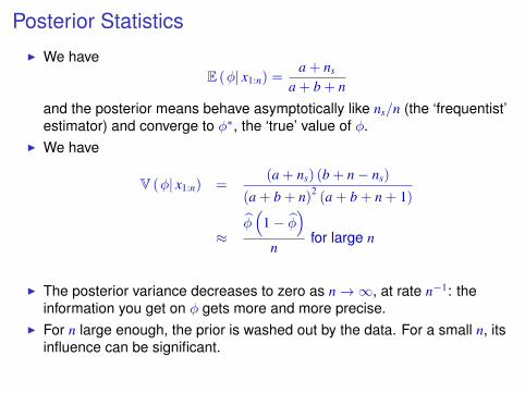
Posterior StatisticsI We have

E (φ| x1:n) =a + ns

a + b + n

and the posterior means behave asymptotically like ns/n (the ‘frequentist’estimator) and converge to φ∗, the ‘true’ value of φ.

I We have

V (φ| x1:n) =(a + ns) (b + n− ns)

(a + b + n)2

(a + b + n + 1)

≈φ(

1− φ)

nfor large n

I The posterior variance decreases to zero as n→∞, at rate n−1: theinformation you get on φ gets more and more precise.

I For n large enough, the prior is washed out by the data. For a small n, itsinfluence can be significant.

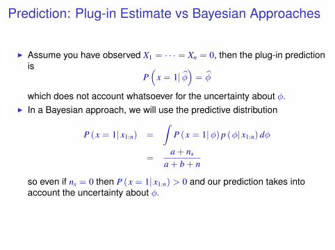
Prediction: Plug-in Estimate vs Bayesian Approaches

I Assume you have observed X1 = · · · = Xn = 0, then the plug-in predictionis

P(

x = 1| φ)

= φ

which does not account whatsoever for the uncertainty about φ.I In a Bayesian approach, we will use the predictive distribution

P (x = 1| x1:n) =

∫P (x = 1|φ) p (φ| x1:n) dφ

=a + ns

a + b + n

so even if ns = 0 then P (x = 1| x1:n) > 0 and our prediction takes intoaccount the uncertainty about φ.

Beta Posteriors

01

02

03

04

05

06

07

08

09

10

11

12

13

14

15

16

17

18

19

20

21

22

23

24

25

26

27

28

29

30

31

32

33

34

35

36

37

38

39

40

41

42

43

44

45

46

47

48

49

50

51

52

53

54

55

56

57

58

59

60

61

bayesBody.tex 129

0 1 2 3 4 5 6 7 8 9 100

0.02

0.04

0.06

0.08

0.1

0.12

0.14prior predictive

(a)

0 1 2 3 4 5 6 7 8 9 100

0.05

0.1

0.15

0.2

0.25

0.3

0.35posterior predictive

(b)

0 1 2 3 4 5 6 7 8 9 100

0.05

0.1

0.15

0.2

0.25

0.3

0.35plugin predictive

(c)

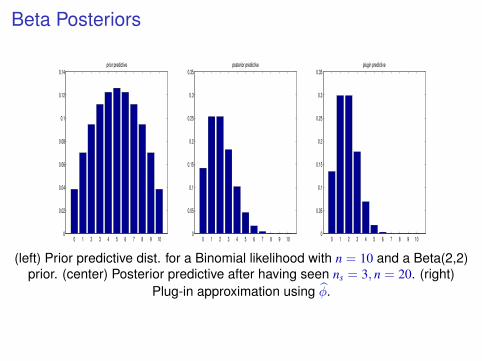
Figure 4.12: (a) Prior predictive distribution for a Binomial likelihood withM = 10 trials, and a Beta(2,2) prior on θ. (b) Posterior predictivedistributions after seeing N1 = 3, N2 = 17. (c) Plugin approximation. Figure generated by betaBinomPostPredDemo.

This distribution has the following mean and variance

E [x] = Mα1

α1 + α2(4.52)

var [x] =Mα1α2

(α1 + α2)2

(α1 + α2 +M)

α1 + α2 + 1(4.53)

If M = 1, and hence x ∈ {0, 1}, we see that the mean becomes

E [x|D] = p(x = 1|D) =α1

α1 + α2(4.54)

which is consistent with Equation 4.46.This process is illustrated in Figure 4.12, where we plot prior predictive density, p(x), under a Beta(2,2) prior, as well as

the posterior predictive density after seeing N1 = 3 heads and N2 = 17 tails. Figure 4.12(c) plots a plug-in approximationusing a MAP estimate. We see that the Bayesian prediction has longer tails, spreading its probablity mass more widely, and istherefore less prone to overfitting and black-swan type paradoxes.

4.5.2 The Dirichlet-multinomial modelWe can generalize the above results from coins to dice in a straightforward fashion, as we now show.

4.5.2.1 Likelihood

From Section 3.2.3, the likelihood has the form

p(D|θ) =K∏

k=1

θNkk (4.55)

where Nk =∑Ni=1 I(yi = k) is the number of times event k occured.

4.5.2.2 Prior

The conjugate prior is the Dirichlet distribution4, which is the natural generalization of the beta distribution to multipledimensions. The pdf is defined as follows:

Dir(θ|α) :=1

B(α)

K∏

k=1

θαk−1k I(x ∈ SK) (4.56)

where SK is the K-dimensional probability simplex, which is the set of vectors such that 0 ≤ θk ≤ 1 and∑Kk=1 θk = 1. In

addition, B(α1, . . . , αK) is the natural generalization of the beta function to K variables:

B(α) :=

∏Ki=1 Γ(αi)

Γ(α0)(4.57)

4Johann Dirichlet was a German mathematician, 1805–1859.

Machine Learning: a Probabilistic Approach, draft of January 4, 2011

(left) Prior predictive dist. for a Binomial likelihood with n = 10 and a Beta(2,2)prior. (center) Posterior predictive after having seen ns = 3, n = 20. (right)

Plug-in approximation using φ.

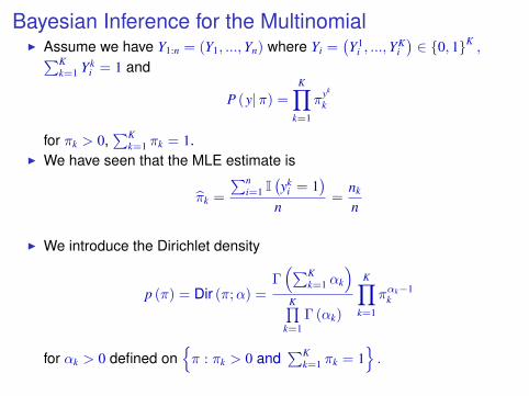
Bayesian Inference for the MultinomialI Assume we have Y1:n = (Y1, ...,Yn) where Yi =

(Y1

i , ...,YKi

)∈ {0, 1}K

,∑Kk=1 Yk

i = 1 and

P (y|π) =

K∏

k=1

πyk

k

for πk > 0,∑K

k=1 πk = 1.I We have seen that the MLE estimate is

πk =

∑ni=1 I

(yk

i = 1)

n=

nk

n

I We introduce the Dirichlet density

p (π) = Dir (π;α) =Γ(∑K

k=1 αk

)

K∏k=1

Γ (αk)

K∏

k=1

παk−1k

for αk > 0 defined on{π : πk > 0 and

∑Kk=1 πk = 1

}.

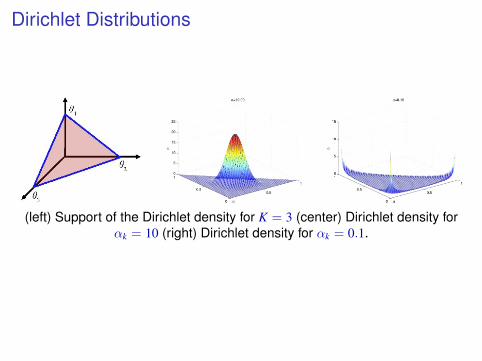
Dirichlet Distributions

(left) Support of the Dirichlet density for K = 3 (center) Dirichlet density forαk = 10 (right) Dirichlet density for αk = 0.1.

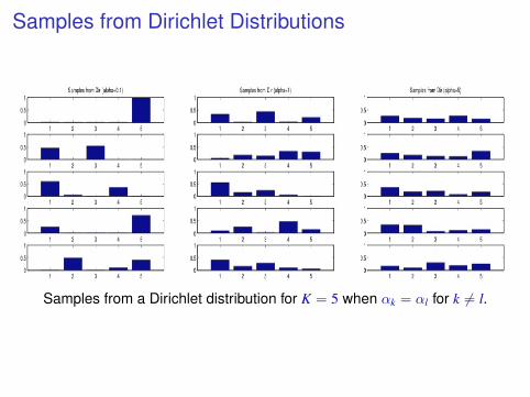
Samples from Dirichlet Distributions

Samples from a Dirichlet distribution for K = 5 when αk = αl for k 6= l.

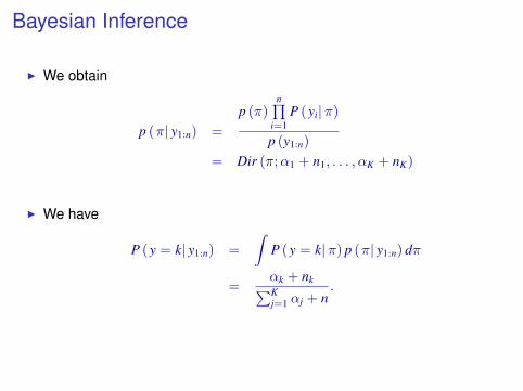
Bayesian Inference

I We obtain

p (π| y1:n) =

p (π)n∏

i=1P (yi|π)

p (y1:n)

= Dir (π;α1 + n1, . . . , αK + nK)

I We have

P (y = k| y1:n) =

∫P (y = k|π) p (π| y1:n) dπ

=αk + nk∑Kj=1 αj + n

.

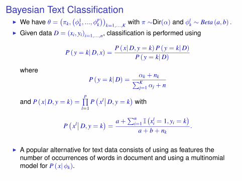
Bayesian Text ClassificationI We have θ =

(πk,(φ1

k , ..., φpk

))k=1,...,K with π ∼Dir(α) and φl

k ∼ Beta (a, b) .

I Given data D = (xi, yi)i=1,...,n, classification is performed using

P (y = k|D, x) =P (x|D, y = k) P (y = k|D)

P (y = k|D)

whereP (y = k|D) =

αk + nk∑Kj=1 αj + n

and P (x|D, y = k) =p∏

l=1P(

xl∣∣D, y = k

)with

P(

xl∣∣D, y = k

)=

a +∑n

i=1 I(xl

i = 1, yi = k)

a + b + nk.

I A popular alternative for text data consists of using as features thenumber of occurrences of words in document and using a multinomialmodel for P (x|φk).

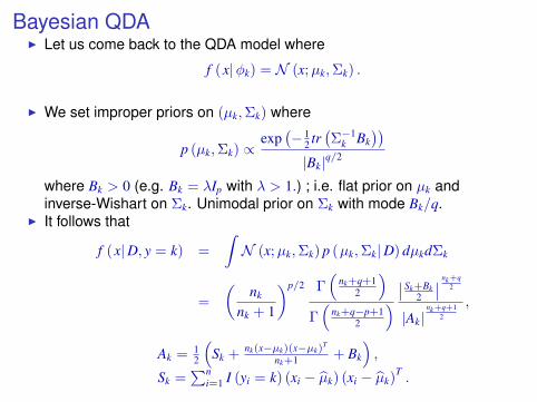
Bayesian QDAI Let us come back to the QDA model where

f (x|φk) = N (x;µk,Σk) .

I We set improper priors on (µk,Σk) where

p (µk,Σk) ∝exp

(− 1

2 tr(Σ−1

k Bk))

|Bk|q/2

where Bk > 0 (e.g. Bk = λIp with λ > 1.) ; i.e. flat prior on µk andinverse-Wishart on Σk. Unimodal prior on Σk with mode Bk/q.

I It follows that

f (x|D, y = k) =

∫N (x;µk,Σk) p (µk,Σk|D) dµkdΣk

=

(nk

nk + 1

)p/2 Γ(

nk+q+12

)

Γ(

nk+q−p+12

)∣∣ Sk+Bk

2

∣∣nk+q

2

|Ak|nk+q+1

2

,

Ak = 12

(Sk + nk(x−µk)(x−µk)

T

nk+1 + Bk

),

Sk =∑n

i=1 I (yi = k) (xi − µk) (xi − µk)T.

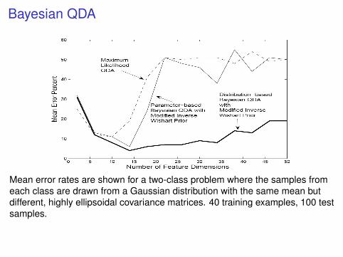
Bayesian QDA

Mean error rates are shown for a two-class problem where the samples fromeach class are drawn from a Gaussian distribution with the same mean butdifferent, highly ellipsoidal covariance matrices. 40 training examples, 100 testsamples.

Outline


Logistic Regression

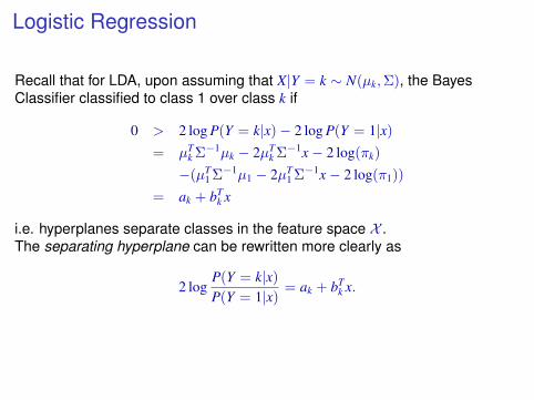
Recall that for LDA, upon assuming that X|Y = k ∼ N(µk,Σ), the BayesClassifier classified to class 1 over class k if

0 > 2 log P(Y = k|x)− 2 log P(Y = 1|x)

= µTk Σ−1µk − 2µT

k Σ−1x− 2 log(πk)

−(µT1 Σ−1µ1 − 2µT

1 Σ−1x− 2 log(π1))

= ak + bTk x

i.e. hyperplanes separate classes in the feature space X .The separating hyperplane can be rewritten more clearly as

2 logP(Y = k|x)

P(Y = 1|x)= ak + bT

k x.

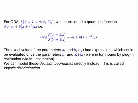
For QDA, X|Y = k ∼ N(µk,Σk), we in turn found a quadratic function0 > ak + bT

k x + xTckx i.e.

2 logP(Y = k|x)

P(Y = 1|x)= ak + bT

k x + xTckx.

The exact value of the parameters ak and bk (ck) had expressions which couldbe evaluated once the parameters µk and Σ (Σk) were in turn found by plug-inestimation (via ML estimation)We can model these decision boundaries directly instead. This is calledlogistic discrimination.

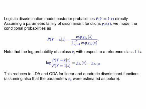
Logistic discrimination model posterior probabilities P(Y = k|x) directly.Assuming a parametric family of discriminant functions gβ(x), we model theconditional probabilities as

P(Y = k|x) =exp gβk (x)∑Kj=1 exp gβj(x)

.

Note that the log probability of a class k, with respect to a reference class 1 is:

logP(Y = k|x)

P(Y = 1|x)= gβk (x)− gβ1(x)

This reduces to LDA and QDA for linear and quadratic discriminant functions(assuming also that the parameters βk were estimated as before).

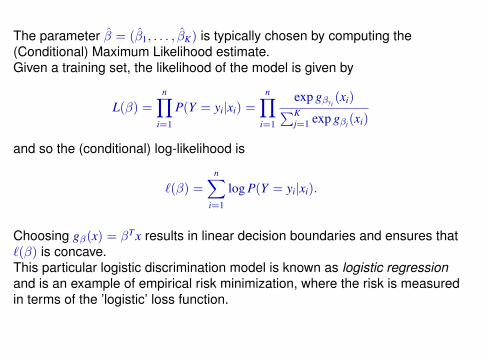
The parameter β = (β1, . . . , βK) is typically chosen by computing the(Conditional) Maximum Likelihood estimate.Given a training set, the likelihood of the model is given by

L(β) =

n∏

i=1

P(Y = yi|xi) =

n∏

i=1

exp gβyi(xi)∑K

j=1 exp gβj(xi)

and so the (conditional) log-likelihood is

`(β) =

n∑

i=1

log P(Y = yi|xi).

Choosing gβ(x) = βTx results in linear decision boundaries and ensures that`(β) is concave.This particular logistic discrimination model is known as logistic regressionand is an example of empirical risk minimization, where the risk is measuredin terms of the ’logistic’ loss function.

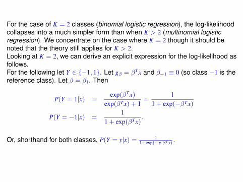
For the case of K = 2 classes (binomial logistic regression), the log-likelihoodcollapses into a much simpler form than when K > 2 (multinomial logisticregression). We concentrate on the case where K = 2 though it should benoted that the theory still applies for K > 2.Looking at K = 2, we can derive an explicit expression for the log-likelihood asfollows.For the following let Y ∈ {−1, 1}. Let gβ = βTx and β−1 ≡ 0 (so class −1 is thereference class). Let β = β1. Then

P(Y = 1|x) =exp(βTx)

exp(βTx) + 1=

11 + exp(−βTx)

P(Y = −1|x) =1

1 + exp(βTx).

Or, shorthand for both classes, P(Y = y|x) = 11+exp(−y·βT x) .

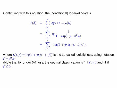
Continuing with this notation, the (conditional) log-likelihood is

`(β) =

n∑

i=1

log P(Y = yi|xi)

=

n∑

i=1

log1

1 + exp(−yi · βTxi)

=

n∑

i=1

− log(1 + exp(−yi · βTxi)),

where L(y, f ) = log(1 + exp(−y · f )) is the so-called logistic loss, using notationf = βTxi.(Note that for under 0-1 loss, the optimal classification is 1 if f > 0 and -1 iff ≤ 0.)

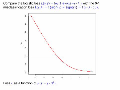
Compare the logistic loss L(y, f ) = log(1 + exp(−y · f )) with the 0-1misclassification loss L(y, f ) = 1{sign(y) 6= sign(f )} = 1{y · f < 0}.

!3 !2 !1 0 1 2 3

0.0

0.5

1.0

1.5

2.0

2.5

3.0

3.5

f

Loss

Loss L as a function of y · f = y · βTx.

As shown above, ML estimation is (in the case Y ∈ {−1, 1} equivalent tosolving the equations),

β = argminβn∑

i=1

log(1 + exp(−yi · βTxi)),

numerical methods must be applied. A high-dimensional version of theNewton-Raphson algorithm is typically used, where locally the objectivefunction is approximated by a quadratic function and the solution is then foundby iterated least squares.When using the univariate Newton-Raphson approach, we need informationabout the slope of the curve, in our case we need the Hessian matrix

∂2`(β)

∂β∂βT = −n∑

i=1

xixTi p(xi|β) [1− p(xi|β)] .

Extending Newton-Raphson to higher dimensions, starting with βold, a singleNewton-Raphson update is given by

βnew = βold −(∂2`(β)

∂β∂βT

)−1∂`(β)

∂β

where the derivatives are evaluated at βold.

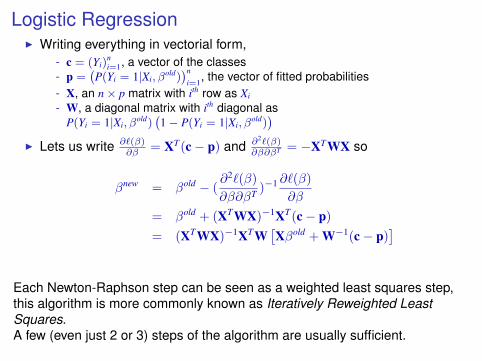
Logistic RegressionI Writing everything in vectorial form,

- c = (Yi)ni=1, a vector of the classes

- p =(P(Yi = 1|Xi, β

old))n

i=1, the vector of fitted probabilities

- X, an n× p matrix with ith row as Xi

- W, a diagonal matrix with ith diagonal asP(Yi = 1|Xi, β

old)(1− P(Yi = 1|Xi, β

old))

I Lets us write ∂`(β)∂β = XT(c− p) and ∂2`(β)

∂β∂βT = −XTWX so

βnew = βold − (∂2`(β)

∂β∂βT )−1 ∂`(β)

∂β

= βold + (XTWX)−1XT(c− p)

= (XTWX)−1XTW[Xβold + W−1(c− p)

]

Each Newton-Raphson step can be seen as a weighted least squares step,this algorithm is more commonly known as Iteratively Reweighted LeastSquares.A few (even just 2 or 3) steps of the algorithm are usually sufficient.

Example: O-ring failures during shuttle starts (preceeeding the Challengerincident), as a function of temperatures.

library(alr3)data(challeng)temp <- challeng[,1]failure <- challeng[,3]Y <- as.numeric(failure>0)

plot(temp,Y,xlab="TEMPERATURE",ylab="O-RING FAILURES",cex=2)

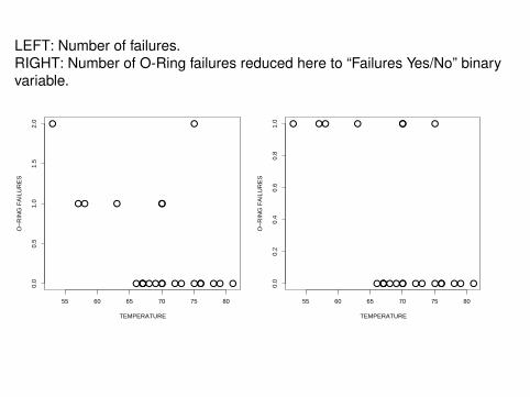
LEFT: Number of failures.RIGHT: Number of O-Ring failures reduced here to “Failures Yes/No” binaryvariable.

●

●● ●

●●●●●●

●

●

●

● ●● ●

●

●● ●● ●

55 60 65 70 75 80

0.0

0.5

1.0

1.5

2.0

TEMPERATURE

O−

RIN

G F

AIL

UR

ES

● ●● ●

●●●●●●

●

●

●

● ●● ●

●

●● ●● ●

55 60 65 70 75 80

0.0

0.2

0.4

0.6

0.8

1.0

TEMPERATURE

O−

RIN

G F

AIL

UR

ES

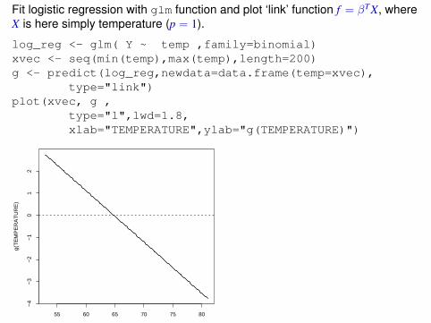
Fit logistic regression with glm function and plot ‘link’ function f = βTX, whereX is here simply temperature (p = 1).

log_reg <- glm( Y ~ temp ,family=binomial)xvec <- seq(min(temp),max(temp),length=200)g <- predict(log_reg,newdata=data.frame(temp=xvec),

type="link")plot(xvec, g ,

type="l",lwd=1.8,xlab="TEMPERATURE",ylab="g(TEMPERATURE)")

55 60 65 70 75 80

−4

−3

−2

−1

01

2

TEMPERATURE

g(T

EM

PE

RA

TU

RE

)

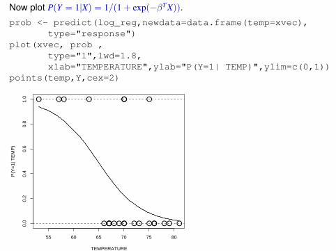
Now plot P(Y = 1|X) = 1/(1 + exp(−βTX)).

prob <- predict(log_reg,newdata=data.frame(temp=xvec),type="response")

plot(xvec, prob ,type="l",lwd=1.8,xlab="TEMPERATURE",ylab="P(Y=1| TEMP)",ylim=c(0,1))

points(temp,Y,cex=2)

55 60 65 70 75 80

0.0

0.2

0.4

0.6

0.8

1.0

TEMPERATURE

P(Y

=1|

TE

MP

)

● ●● ●

●●●●●●

●

●

●

● ●● ●

●

●● ●● ●

Logistic Regression or LDA?

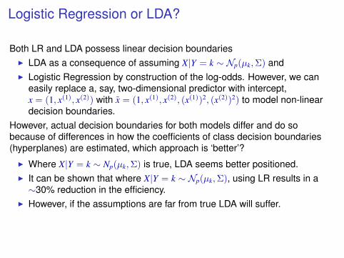
Both LR and LDA possess linear decision boundariesI LDA as a consequence of assuming X|Y = k ∼ Np(µk,Σ) andI Logistic Regression by construction of the log-odds. However, we can

easily replace a, say, two-dimensional predictor with intercept,x = (1, x(1), x(2)) with x = (1, x(1), x(2), (x(1))2, (x(2))2) to model non-lineardecision boundaries.

However, actual decision boundaries for both models differ and do sobecause of differences in how the coefficients of class decision boundaries(hyperplanes) are estimated, which approach is ‘better’?

I Where X|Y = k ∼ Np(µk,Σ) is true, LDA seems better positioned.I It can be shown that where X|Y = k ∼ Np(µk,Σ), using LR results in a∼30% reduction in the efficiency.

I However, if the assumptions are far from true LDA will suffer.

In support of Logistic Regression over LDA, it can be noted that LogisticRegression is simply a generalised linear model (GLM).Knowing this, we can take advantage of all of the theory developed for GLMs.

I assessment of fit via deviance and plots,I interpretation of βk’s via odds-ratios,I fitting categorical data (code it via indicator functions),I well founded approaches to removing insignificant terms (via the drop-in

deviance test and the Wald test),I model selection via AIC/BIC.

Ultimately, we have to let the data speak!

Spam dataset: Look at examples of spam emails and non-spam emails. Thepredictor variables count occurrence of specific words/characters. Look at thefirst 2 emails in the database (which are spam).> library(kernlab)> data(spam)> dim(spam)[1] 4601 58

> spam[1:2,]make address all num3d our over remove internet order mail receive will

1 0.00 0.64 0.64 0 0.32 0.00 0.00 0.00 0 0.00 0.00 0.642 0.21 0.28 0.50 0 0.14 0.28 0.21 0.07 0 0.94 0.21 0.79people report addresses free business email you credit your font num000

1 0.00 0.00 0.00 0.32 0.00 1.29 1.93 0 0.96 0 0.002 0.65 0.21 0.14 0.14 0.07 0.28 3.47 0 1.59 0 0.43money hp hpl george num650 lab labs telnet num857 data num415 num85

1 0.00 0 0 0 0 0 0 0 0 0 0 02 0.43 0 0 0 0 0 0 0 0 0 0 0technology num1999 parts pm direct cs meeting original project re edu table

1 0 0.00 0 0 0 0 0 0 0 0 0 02 0 0.07 0 0 0 0 0 0 0 0 0 0conference charSemicolon charRoundbracket charSquarebracket charExclamation

1 0 0 0.000 0 0.7782 0 0 0.132 0 0.372charDollar charHash capitalAve capitalLong capitalTotal type

1 0.00 0.000 3.756 61 278 spam2 0.18 0.048 5.114 101 1028 spam>

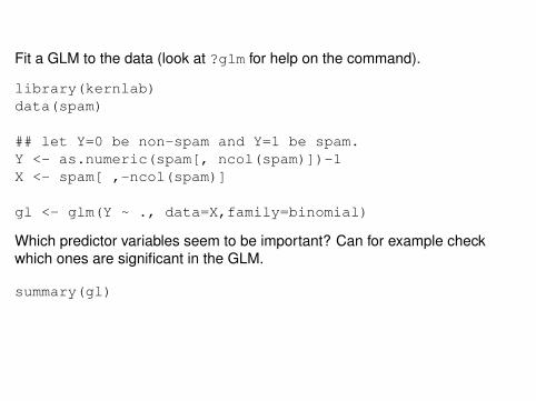
Fit a GLM to the data (look at ?glm for help on the command).

library(kernlab)data(spam)

## let Y=0 be non-spam and Y=1 be spam.Y <- as.numeric(spam[, ncol(spam)])-1X <- spam[ ,-ncol(spam)]

gl <- glm(Y ~ ., data=X,family=binomial)

Which predictor variables seem to be important? Can for example checkwhich ones are significant in the GLM.

summary(gl)

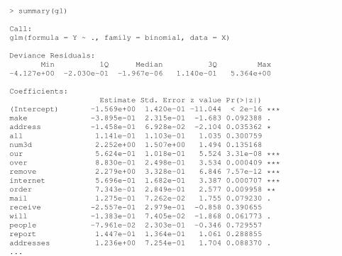
> summary(gl)

Call:glm(formula = Y ~ ., family = binomial, data = X)

Deviance Residuals:Min 1Q Median 3Q Max

-4.127e+00 -2.030e-01 -1.967e-06 1.140e-01 5.364e+00

Coefficients:Estimate Std. Error z value Pr(>|z|)

(Intercept) -1.569e+00 1.420e-01 -11.044 < 2e-16 ***make -3.895e-01 2.315e-01 -1.683 0.092388 .address -1.458e-01 6.928e-02 -2.104 0.035362 *all 1.141e-01 1.103e-01 1.035 0.300759num3d 2.252e+00 1.507e+00 1.494 0.135168our 5.624e-01 1.018e-01 5.524 3.31e-08 ***over 8.830e-01 2.498e-01 3.534 0.000409 ***remove 2.279e+00 3.328e-01 6.846 7.57e-12 ***internet 5.696e-01 1.682e-01 3.387 0.000707 ***order 7.343e-01 2.849e-01 2.577 0.009958 **mail 1.275e-01 7.262e-02 1.755 0.079230 .receive -2.557e-01 2.979e-01 -0.858 0.390655will -1.383e-01 7.405e-02 -1.868 0.061773 .people -7.961e-02 2.303e-01 -0.346 0.729557report 1.447e-01 1.364e-01 1.061 0.288855addresses 1.236e+00 7.254e-01 1.704 0.088370 ....

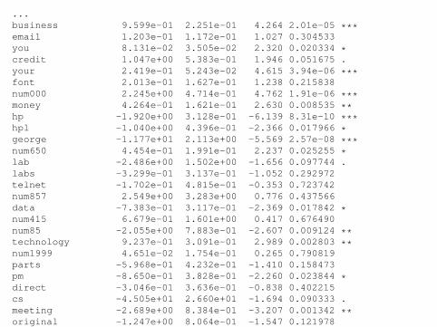
...business 9.599e-01 2.251e-01 4.264 2.01e-05 ***email 1.203e-01 1.172e-01 1.027 0.304533you 8.131e-02 3.505e-02 2.320 0.020334 *credit 1.047e+00 5.383e-01 1.946 0.051675 .your 2.419e-01 5.243e-02 4.615 3.94e-06 ***font 2.013e-01 1.627e-01 1.238 0.215838num000 2.245e+00 4.714e-01 4.762 1.91e-06 ***money 4.264e-01 1.621e-01 2.630 0.008535 **hp -1.920e+00 3.128e-01 -6.139 8.31e-10 ***hpl -1.040e+00 4.396e-01 -2.366 0.017966 *george -1.177e+01 2.113e+00 -5.569 2.57e-08 ***num650 4.454e-01 1.991e-01 2.237 0.025255 *lab -2.486e+00 1.502e+00 -1.656 0.097744 .labs -3.299e-01 3.137e-01 -1.052 0.292972telnet -1.702e-01 4.815e-01 -0.353 0.723742num857 2.549e+00 3.283e+00 0.776 0.437566data -7.383e-01 3.117e-01 -2.369 0.017842 *num415 6.679e-01 1.601e+00 0.417 0.676490num85 -2.055e+00 7.883e-01 -2.607 0.009124 **technology 9.237e-01 3.091e-01 2.989 0.002803 **num1999 4.651e-02 1.754e-01 0.265 0.790819parts -5.968e-01 4.232e-01 -1.410 0.158473pm -8.650e-01 3.828e-01 -2.260 0.023844 *direct -3.046e-01 3.636e-01 -0.838 0.402215cs -4.505e+01 2.660e+01 -1.694 0.090333 .meeting -2.689e+00 8.384e-01 -3.207 0.001342 **original -1.247e+00 8.064e-01 -1.547 0.121978project -1.573e+00 5.292e-01 -2.973 0.002953 **re -7.923e-01 1.556e-01 -5.091 3.56e-07 ***edu -1.459e+00 2.686e-01 -5.434 5.52e-08 ***table -2.326e+00 1.659e+00 -1.402 0.160958conference -4.016e+00 1.611e+00 -2.493 0.012672 *charSemicolon -1.291e+00 4.422e-01 -2.920 0.003503 **charRoundbracket -1.881e-01 2.494e-01 -0.754 0.450663charSquarebracket -6.574e-01 8.383e-01 -0.784 0.432914charExclamation 3.472e-01 8.926e-02 3.890 0.000100 ***charDollar 5.336e+00 7.064e-01 7.553 4.24e-14 ***charHash 2.403e+00 1.113e+00 2.159 0.030883 *capitalAve 1.199e-02 1.884e-02 0.636 0.524509capitalLong 9.118e-03 2.521e-03 3.618 0.000297 ***capitalTotal 8.437e-04 2.251e-04 3.747 0.000179 ***---Signif. codes: 0 ’***’ 0.001 ’**’ 0.01 ’*’ 0.05 ’.’ 0.1 ’ ’ 1

(Dispersion parameter for binomial family taken to be 1)

Null deviance: 6170.2 on 4600 degrees of freedomResidual deviance: 1815.8 on 4543 degrees of freedomAIC: 1931.8

Number of Fisher Scoring iterations: 13

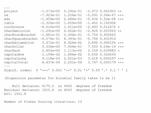
...project -1.573e+00 5.292e-01 -2.973 0.002953 **re -7.923e-01 1.556e-01 -5.091 3.56e-07 ***edu -1.459e+00 2.686e-01 -5.434 5.52e-08 ***table -2.326e+00 1.659e+00 -1.402 0.160958conference -4.016e+00 1.611e+00 -2.493 0.012672 *charSemicolon -1.291e+00 4.422e-01 -2.920 0.003503 **charRoundbracket -1.881e-01 2.494e-01 -0.754 0.450663charSquarebracket -6.574e-01 8.383e-01 -0.784 0.432914charExclamation 3.472e-01 8.926e-02 3.890 0.000100 ***charDollar 5.336e+00 7.064e-01 7.553 4.24e-14 ***charHash 2.403e+00 1.113e+00 2.159 0.030883 *capitalAve 1.199e-02 1.884e-02 0.636 0.524509capitalLong 9.118e-03 2.521e-03 3.618 0.000297 ***capitalTotal 8.437e-04 2.251e-04 3.747 0.000179 ***---Signif. codes: 0 ’***’ 0.001 ’**’ 0.01 ’*’ 0.05 ’.’ 0.1 ’ ’ 1

(Dispersion parameter for binomial family taken to be 1)

Null deviance: 6170.2 on 4600 degrees of freedomResidual deviance: 1815.8 on 4543 degrees of freedomAIC: 1931.8

Number of Fisher Scoring iterations: 13

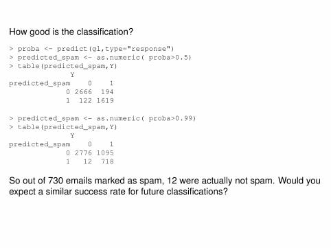
How good is the classification?

> proba <- predict(gl,type="response")> predicted_spam <- as.numeric( proba>0.5)> table(predicted_spam,Y)

Ypredicted_spam 0 1

0 2666 1941 122 1619

> predicted_spam <- as.numeric( proba>0.99)> table(predicted_spam,Y)

Ypredicted_spam 0 1

0 2776 10951 12 718

So out of 730 emails marked as spam, 12 were actually not spam. Would youexpect a similar success rate for future classifications?

Outline


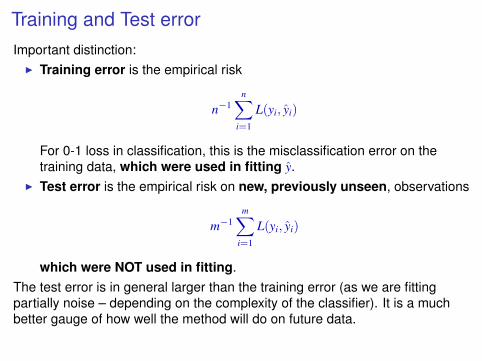
Training and Test errorImportant distinction:

I Training error is the empirical risk

n−1n∑

i=1

L(yi, yi)

For 0-1 loss in classification, this is the misclassification error on thetraining data, which were used in fitting y.

I Test error is the empirical risk on new, previously unseen, observations

m−1m∑

i=1

L(yi, yi)

which were NOT used in fitting.The test error is in general larger than the training error (as we are fittingpartially noise – depending on the complexity of the classifier). It is a muchbetter gauge of how well the method will do on future data.

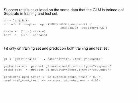
Success rate is calculated on the same data that the GLM is trained on!Separate in training and test set.

n <- length(Y)intrain <- sample( rep(c(TRUE,FALSE),each=n/2) ,

round(n/2) ,replace=TRUE )train <- (1:n)[intrain]test <- (1:n)[!intrain]

Fit only on training set and predict on both training and test set.

gl <- glm(Y[train] ~ ., data=X[train,],family=binomial)

proba_train <- predict(gl,newdata=X[train,],type="response")proba_test <- predict(gl,newdata=X[test,],type="response")

predicted_spam_train <- as.numeric(proba_train > 0.95)predicted_spam_test <- as.numeric(proba_test > 0.95)

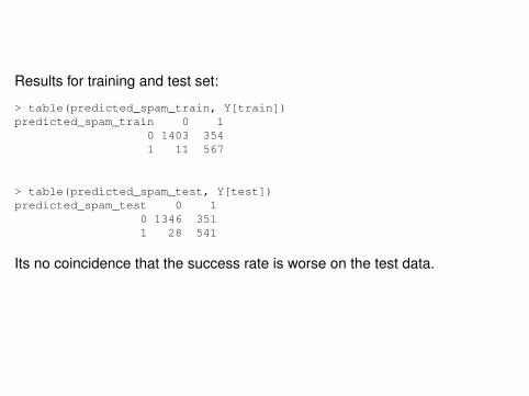
Results for training and test set:

> table(predicted_spam_train, Y[train])predicted_spam_train 0 1

0 1403 3541 11 567

> table(predicted_spam_test, Y[test])predicted_spam_test 0 1

0 1346 3511 28 541

Its no coincidence that the success rate is worse on the test data.

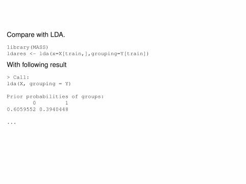
Compare with LDA.

library(MASS)ldares <- lda(x=X[train,],grouping=Y[train])

With following result

> Call:lda(X, grouping = Y)

Prior probabilities of groups:0 1

0.6059552 0.3940448

...

...

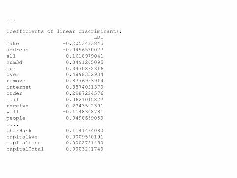
Coefficients of linear discriminants:LD1

make -0.2053433845address -0.0496520077all 0.1618979041num3d 0.0491205095our 0.3470862316over 0.4898352934remove 0.8776953914internet 0.3874021379order 0.2987224576mail 0.0621045827receive 0.2343512301will -0.1148308781people 0.0490659059....charHash 0.1141464080capitalAve 0.0009590191capitalLong 0.0002751450capitalTotal 0.0003291749

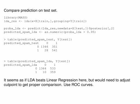
Compare prediction on test set.

library(MASS)lda_res <- lda(x=X[train,],grouping=Y[train])

proba_lda <- predict(lda_res,newdata=X[test,])$posterior[,2]predicted_spam_lda <- as.numeric(proba_lda > 0.95)

> table(predicted_spam_test, Y[test])predicted_spam_test 0 1

0 1346 3511 28 541

> table(predicted_spam_lda, Y[test])predicted_spam_lda 0 1

0 1364 5331 10 359

It seems as if LDA beats Linear Regression here, but would need to adjustcutpoint to get proper comparison. Use ROC curves.

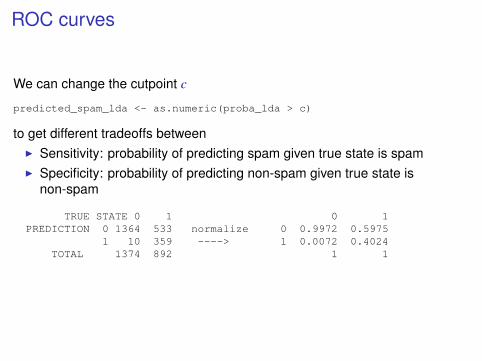
ROC curves

We can change the cutpoint c

predicted_spam_lda <- as.numeric(proba_lda > c)

to get different tradeoffs betweenI Sensitivity: probability of predicting spam given true state is spamI Specificity: probability of predicting non-spam given true state is

non-spam

TRUE STATE 0 1 0 1PREDICTION 0 1364 533 normalize 0 0.9972 0.5975

1 10 359 ----> 1 0.0072 0.4024TOTAL 1374 892 1 1

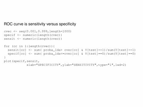
ROC curve is sensitivity versus specificity

cvec <- seq(0.001,0.999,length=1000)specif <- numeric(length(cvec))sensit <- numeric(length(cvec))

for (cc in 1:length(cvec)){sensit[cc] <- sum( proba_lda> cvec[cc] & Y[test]==1)/sum(Y[test]==1)specif[cc] <- sum( proba_lda<=cvec[cc] & Y[test]==0)/sum(Y[test]==0)

}plot(specif,sensit,

xlab="SPECIFICITY",ylab="SENSITIVITY",type="l",lwd=2)

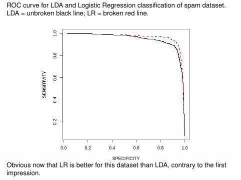
ROC curve for LDA and Logistic Regression classification of spam dataset.LDA = unbroken black line; LR = broken red line.

0.0 0.2 0.4 0.6 0.8 1.0

0.2

0.4

0.6

0.8

1.0

SPECIFICITY

SE

NS

ITIV

ITY

Obvious now that LR is better for this dataset than LDA, contrary to the firstimpression.