M.S. Thesis - OAKTrust - Texas A&M University

EXPERIMENTAL CONTRIBUTION ANALYSIS OF EXTERNAL NOISE

COMPONENTS TO THE INTERIOR NOISE OF AN AUTOMOBILE

A Thesis

by

SEONGIL HWANG

Submitted to the Office of Graduate and Professional Studies of

Texas A&M University

in partial fulfillment of the requirements for the degree of

MASTER OF SCIENCE

Chair of Committee, Yong-Joe Kim

Committee Members, Edward B. White

Luis San Andres

Head of Department, Andreas A. Polycarpou

December 2016

Major Subject: Mechanical Engineering

Copyright 2016 Seongil Hwang

ii

ABSTRACT

The contribution analysis of various noise sources in the automobile interior

noise is important for a well-designed vehicle with a low interior noise level. The

proposed modified Cholesky Decomposition (CD) is able to decompose the interior

noise spectra into multiple spectra, each physically representing the contribution of a

specific noise source to the interior noise of the automobile. During an experiment with

two speakers driven by two independent white noise signals, it is shown that the

measured noise spectrum can be successfully decomposed into two contributions, each

associated with noise radiated from speakers.

Then, a simplified, scaled automobile model (with one side mirror, one front and

two side windows, and flat top, back, and bottom panels) was tested in a wind tunnel at

the airflow speeds of 15 m/s (54 km/h) and 24 m/s (86.4 km/h). In this experiment, 14

external and 1 interior microphones were implemented to measure the external

aeroacoustic source signals and the interior noise signal respectively. The results

obtained by processing the microphone signals reveal the contributions of the external

aeroacoustic noise sources to the interior noise.

In addition, an automobile was tested on a road at the speeds of 104.6 km/h (65

mph, or 29.1 m/s) and 128.7 km/h (80 mph, or 35.8 m/s). In this experiment, 64 exterior

and 4 interior microphones measured the external noise source signals and interior noise

signals, respectively. The results obtained by processing the measured microphone

signals indicated the highest contributor of the external aeroacoustic noises are the

windows and the hood. It was also detected that the contribution of the windows

iii

increased as the speed increased and the highest contribution of the interior noise

occurred to the seat closer to the window.

The proposed CD-based procedure requires installing microphones flush-

mounted on the exterior surface of the automobile to measure the noise source signals.

However, the surface-flush-mounted microphone installation can be labor-intensive and

time-consuming, making it difficult to evaluate a large number of aeroacoustic design

cases. Thus, an innovative, CD-based contribution analysis system integrated with an

exterior microphone array is proposed. In this integrated system, the surface-flush-

mounted microphones are replaced with the exterior microphone arrays. This array-

measurement-based contribution analysis procedure was validated by conducting an

experiment with two speakers and an 8 by 8 array of microphones.

iv

TABLE OF CONTENTS

Page

ABSTRACT .......................................................................................................................ii

TABLE OF CONTENTS .................................................................................................. iv

LIST OF FIGURES ........................................................................................................... vi

LIST OF TABLES ............................................................................................................ ix

1. INTRODUCTION .......................................................................................................... 1

2. CD-BASED CONTRIBUTION ANALYSIS THEORY ............................................... 6

3. EXPERIMENT WITH TWO SPEAKERS .................................................................. 11

3.1 Experimental Setup ................................................................................................ 11

3.2 Results and Discussion ........................................................................................... 12

4. EXPERIMENT WITH SIMPLIFIED, SCALED AUTOMOBILE MODEL .............. 16

4.1 Design Overview .................................................................................................... 16

4.2 Outer Plates ............................................................................................................ 17

4.3 Interior Noise Insulation Materials ........................................................................ 18 4.4 Windows (Glasses) ................................................................................................. 18 4.5 Side Mirror and Rain Gutters ................................................................................. 18

4.6 Supports for Model................................................................................................. 19 4.7 Microphone Fairings .............................................................................................. 19

5. WIND TUNNEL TEST AND RESULTS ................................................................... 21

5.1 Klebanoff-Saric Wind Tunnel ................................................................................ 21

5.2 Experimental Setup for Wind Tunnel Test ............................................................ 21 5.3 Wind Tunnel Test ................................................................................................... 23 5.4 Test Results and Discussion ................................................................................... 25

6. EXPERIMENT WITH AUTOMOBILE AND RESULTS .......................................... 31

6.1 Experimental Setup for Automobile Test............................................................... 31 6.2 Test Results and Discussion ................................................................................... 35

7. MICROPHONE-ARRAY-MEASUREMENT-BASED CONTRIBUTION

ANALYSIS ...................................................................................................................... 40

v

7.1 Identification of Source Locations Using Two Beamforming Methods ................ 41 7.2 Reconstruction of Virtual Source Signals from Measured Array Signals ............. 42 7.3 Experimental Setup for Validation ......................................................................... 43 7.4 Test Results and Discussions ................................................................................. 45

8. CONCLUSIONS .......................................................................................................... 50

REFERENCES ................................................................................................................. 52

APPENDIX ...................................................................................................................... 57

A. Contribution Analysis Software .............................................................................. 57

A.1 Description of CAS ........................................................................................... 58 A.2 Quick instruction. .............................................................................................. 64

vi

LIST OF FIGURES

Page

Figure 1: Overall signal processing procedure. .................................................................. 9

Figure 2: Experimental setup with two speakers: (a) Schematic diagram of equipment

connection and (b) Locations of speakers and microphones, and speaker

excitation signals. ............................................................................................. 11

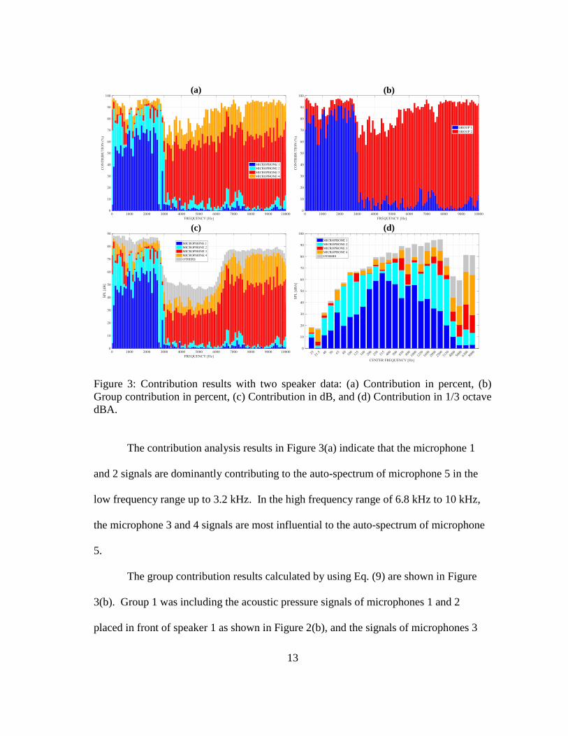
Figure 3: Contribution results with two speaker data: (a) Contribution in percent, (b)

Group contribution in percent, (c) Contribution in dB, and (d) Contribution

in 1/3 octave dBA. ............................................................................................ 13

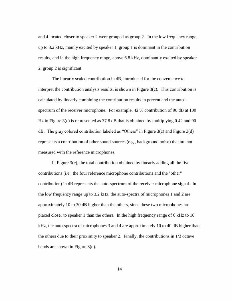
Figure 4: Contribution results with two speaker data: (a) SVD-based contribution, (b)

CD-based contribution. ..................................................................................... 15

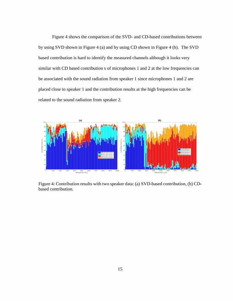
Figure 5: Simplified, scaled automobile model. .............................................................. 16

Figure 6: (a) Supports of model and their covers, (b) Side view of cover, and (c)

Bottom view of cover. ...................................................................................... 19

Figure 7: (a) 3-D printed microphone fairing and (b) Assembled with microphone. ...... 20

Figure 8: Microphone locations in automobile model: (a) Left side view and (b) Top

view. .................................................................................................................. 22

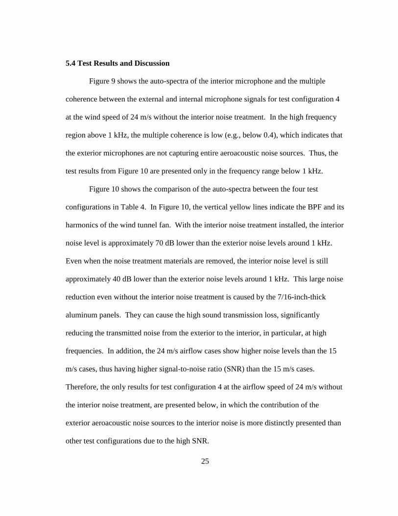
Figure 9: Wind tunnel test results at airflow speed of 24 m/s without interior noise

treatment in frequency range up to 4 kHz. (a) Auto-spectrum of interior

microphone in both wind tunnel test and interior acoustic resonance test and

(b) Multiple coherence between exterior and interior microphone signals in

wind tunnel test. ................................................................................................ 26

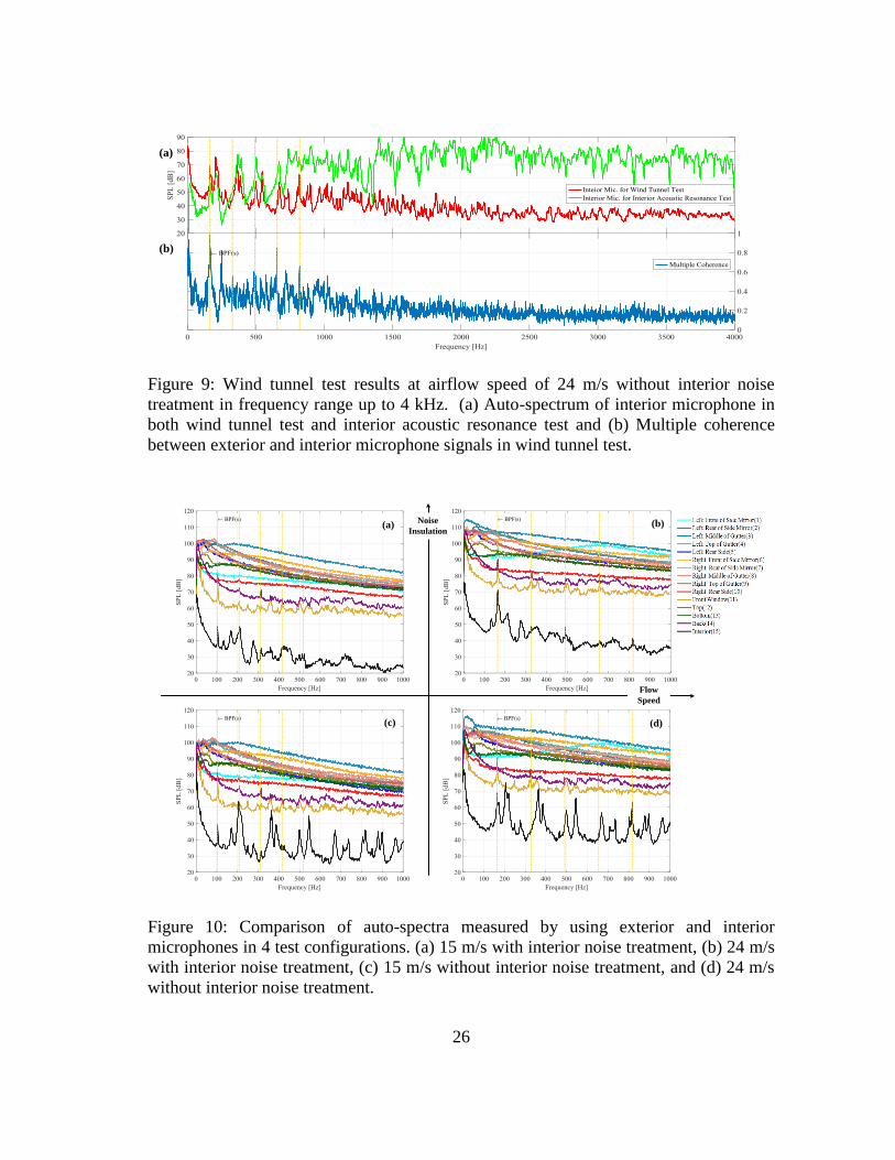
Figure 10: Comparison of auto-spectra measured by using exterior and interior

microphones in 4 test configurations. (a) 15 m/s with interior noise

treatment, (b) 24 m/s with interior noise treatment, (c) 15 m/s without

interior noise treatment, and (d) 24 m/s without interior noise treatment. ....... 26

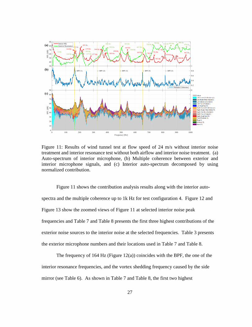
Figure 11: Results of wind tunnel test at flow speed of 24 m/s without interior noise

treatment and interior resonance test without both airflow and interior noise

treatment. (a) Auto-spectrum of interior microphone, (b) Multiple

coherence between exterior and interior microphone signals, and (c) Interior

auto-spectrum decomposed by using normalized contribution. ....................... 27

vii

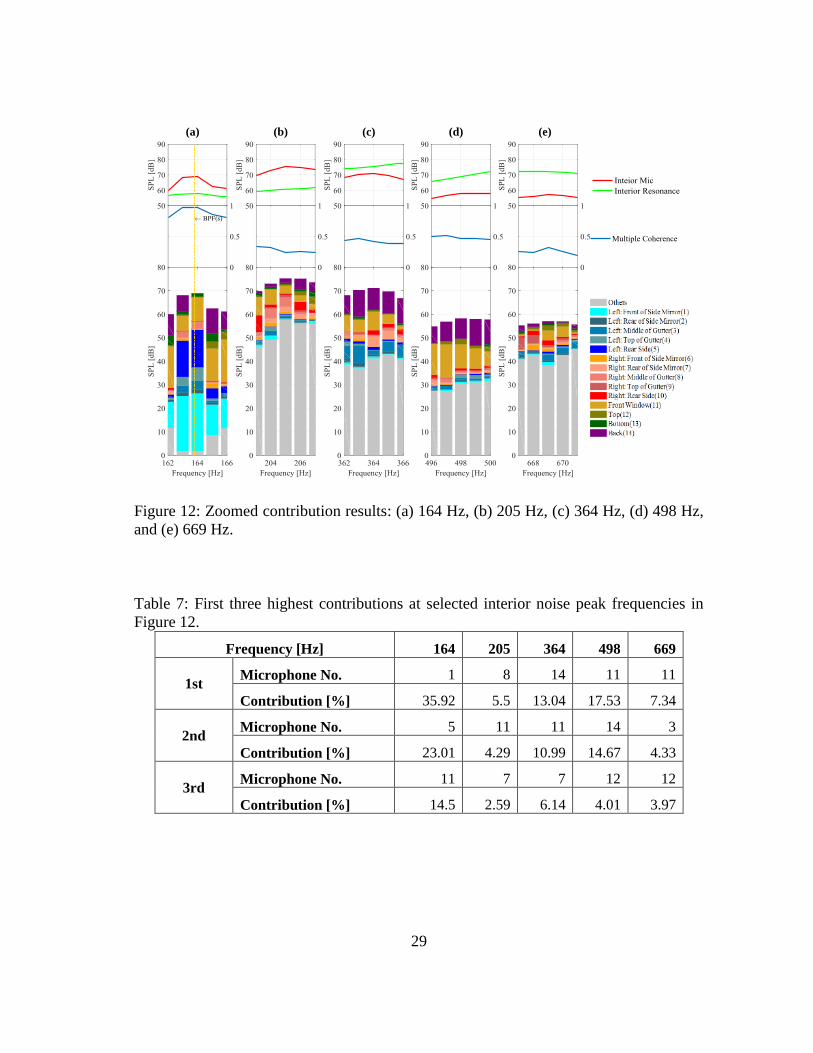
Figure 12: Zoomed contribution results: (a) 164 Hz, (b) 205 Hz, (c) 364 Hz, (d) 498

Hz, and (e) 669 Hz. ........................................................................................... 29

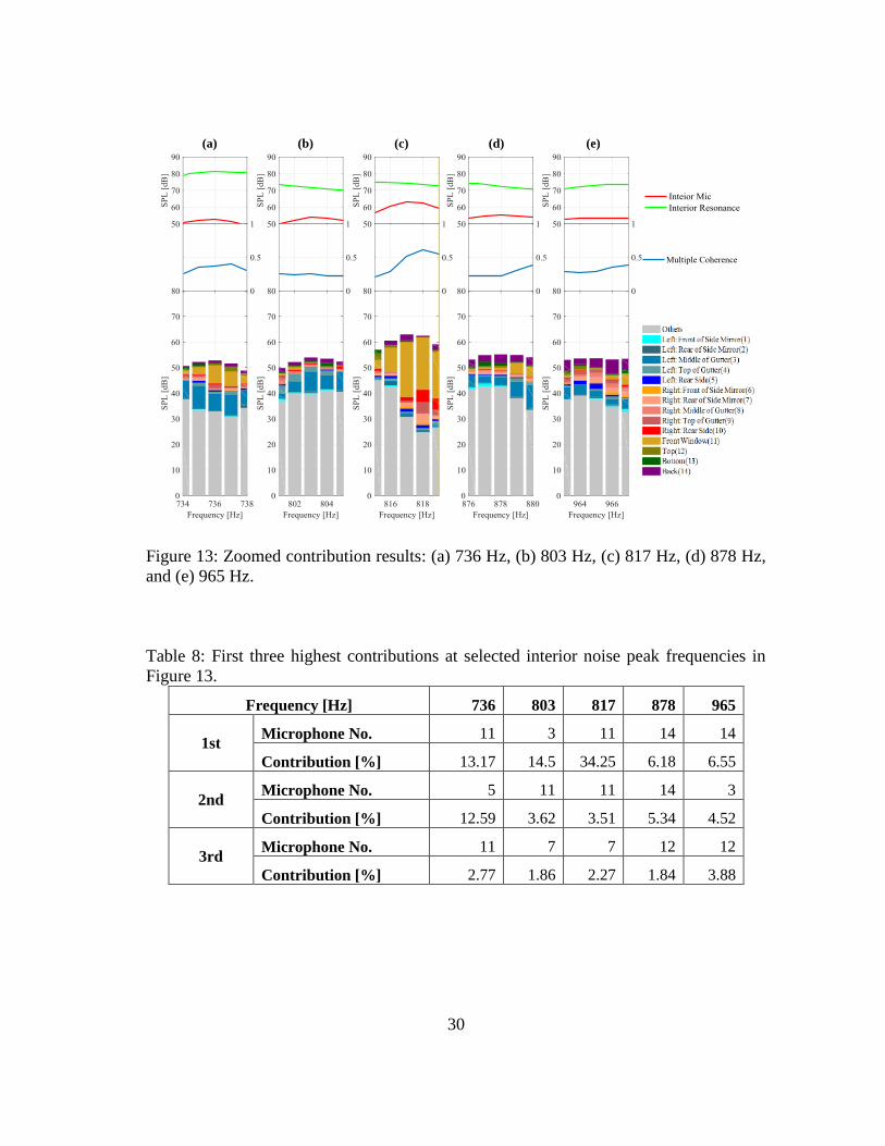
Figure 13: Zoomed contribution results: (a) 736 Hz, (b) 803 Hz, (c) 817 Hz, (d) 878

Hz, and (e) 965 Hz. ........................................................................................... 30

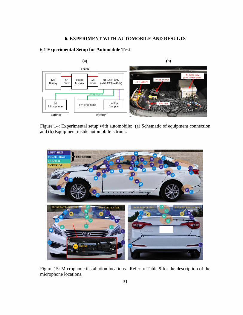
Figure 14: Experimental setup with automobile: (a) Schematic of equipment

connection and (b) Equipment inside automobile’s trunk. ............................... 31

Figure 15: Microphone installation locations. Refer to Table 9 for the description of

the microphone locations. ................................................................................. 31

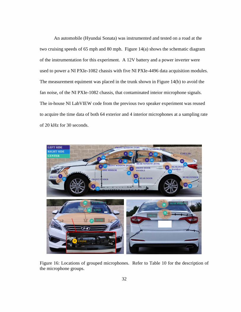
Figure 16: Locations of grouped microphones. Refer to Table 10 for the description

of the microphone groups. ................................................................................ 32

Figure 17: 1/3 octave band contributions of microphone groups (Figure 16 and Table

10) to interior noise at front driver side seat in dBA at automobile speed of

80 mph.. ............................................................................................................ 36

Figure 18: Overall contribution results of microphone groups (Figure 16 and Table

10) to interior noise at front driver side seat at speed of 80 mph. .................... 37

Figure 19: Effects of automobile speeds on overall contribution of microphone groups

(Figure 16 and Table 10) at front driver side seat. ........................................... 38

Figure 20: Effects of seat positions on overall contribution of microphone groups

(Figure 16 and Table 10) at automobile speed of 80 mph. ............................... 39

Figure 21: Scheme of beamforming based contribution analysis. ................................... 40

Figure 22: Experimental setup for validation of beamforming with microphone array

and CD-based contribution analysis procedure: (a) Illustration of

experimental setup, (b) Three speakers with the nine reference

microphones, and (c) the microphone array and receiver microphone placed

at the center of the array. .................................................................................. 44

Figure 23: DAS beamforming powers on the front of the three speakers at different

frequencies: (a) 1 kHz, (b) 1.5 kHz, (c) 2 kHz, (d) 2.5 kHz, (e) 3 kHz, (f)

3.5 kHz, (g) 4 kHz, (h) 4.5 kHz, and (i) 5 kHz. Notes that white lines in the

plot show the locations of the speakers, and speaker units. .............................. 46

Figure 24: MUSIC beamforming powers on the front of the three speakers at different

frequencies: (a) 1 kHz, (b) 1.5 kHz, (c) 2 kHz, (d) 2.5 kHz, (e) 3 kHz, (f)

3.5 kHz, (g) 4 kHz, (h) 4.5 kHz, and (i) 5 kHz. Notes that white lines in the

plot show the locations of the speakers, and speaker units. .............................. 48

viii

Figure 25: Contribution analysis results obtained with real and virtual source signals:

(a) Real source signals measured by using real reference microphones and

(b) Virtual source signals reconstructed by using measured array

microphone signals. .......................................................................................... 49

ix

LIST OF TABLES

Page

Table 1: Three layers of interior noise insulation materials. ............................................ 18

Table 2: Information on Klebanoff-Saric Wind Tunnel (KSWT) [26] at Texas A&M

University. ........................................................................................................ 21

Table 3: Exterior microphone locations (Refer to Figure 8). ........................................... 22

Table 4: Configurations of wind tunnel test and interior acoustic resonance test. ........... 23

Table 5: Two airflow speeds of KSWT and BPFs of fan at two speeds. ......................... 24

Table 6: Frequency range of vortex shedding caused by side mirror. ............................. 24

Table 7: First three highest contributions at selected interior noise peak frequencies in

Figure 12. .......................................................................................................... 29


Figure 13. .......................................................................................................... 30

Table 9: List of noise source microphone locations (Refer to Figure 15). ....................... 33

Table 10: Grouping of noise source microphones (Refer to Figure 16). ......................... 34

1

1. INTRODUCTION*

To design an automobile with low-level interior noise, it is important to analyze

the contribution of various noise sources to the interior noise. Once the contribution of

the noise sources is identified, noise control strategies can be developed based on the

impacts of the noise sources. In general, a noise source with a highest contribution is

targeted foremost, to reduce the overall interior noise level. Here, a novel contribution

analysis technique based on the Cholesky Decomposition (CD) is proposed to

decompose the auto-spectrum of the interior noise into multiple auto-spectra, as a

function of frequency, of which each spectrum, uncorrelated with other spectra,

represents the contribution of a specific noise source to the interior noise. This

contribution analysis can result in physically meaningful decomposition of the interior

noise in association with physical noise sources.

In an automobile, noise is mainly generated from structure-borne and air-borne

noise sources. The structure-borne noises are mainly generated from the structural

vibration, (e.g., of the engine, the transmission, the road/tire). The air-borne noises can

be generated from aerodynamic excitations [1]. As structure-borne noise mitigation

techniques, (e.g., for noise insulation, engine tuning and mounting, and active vibration

control), have been significantly advanced and automobile speed limits have been

increased, exterior aeroacoustic noise sources became critically important as major

* Parts of this section are reprinted from “Experimental contribution analysis of external aeroacoustic noise

components to interior noise of simplified, scaled automobile model in wind tunnel” by Seongil Hwang,

Myunghan Lee, Kang Duck Ih, Edward B. White, and Yong-Joe Kim, 2016, Proceedings of Noise-Con

2016, Providence, RI, United States, Copyright [2016] with permission by NoiseCon 2016 of INCE-USA.

2

contributors to the interior noise. Although the proposed method can be used to analyze

the contribution of any structure-borne and air-borne noise sources, this article focuses

on the aeroacoustic noise sources due to their high contributions to the interior noise of

modern automobiles.

Tcherniak and Schuhmacher [2] summarized existing analysis methods, to

estimate the contributions of automotive noise, vibration, and harshness (NVH) sources,

classifying them into two categories, synthesis and decomposition approaches, based on

how to identify source strengths. One of the most widely-used synthesis approaches is

the Transfer Path Analysis (TPA) [3-4]. The decomposition approaches include the

Multiple Coherence method [5-6], the Operation Transfer Path Analysis (OTPA) [7-13],

and the Transmissibility Matrix Method (TMM) [14-21].

The classical TPA, also known as the Source Path Contribution (SPC) or the

Noise Path Analysis (NPA), requires the measurement of Frequency Response Functions

(FRFs) to determine Transfer Functions (TFs) between input and output points (i.e.,

reference and receiver points) by using impact hammers or shakers for structure-borne

paths or loudspeakers for air-borne paths. Then, synthesized output signals can be

calculated by estimating source strength at each input point and combining the estimated

source strength with the measured FRFs [7]. The limitations of the conventional TPA

are the time-consuming measurement process to obtain the TFs and the errors induced

by the estimated source strengths.

The OTPA first requires experimental data, e.g., interior noise signals and noise

source signals, under operational conditions and measured or estimated TFs in isolated

3

conditions of which each condition has only one source turned on [8-9]. Then, a

Principle Component Analysis (PCA) technique such as the Singular Value

Decomposition (SVD) can be applied to decompose operational source strengths from

the operational data. The operational source strengths can be combined the isolated TFs

to identify the contributions of the sources [8]. The OTPA can be used to address the

main drawbacks of the classical TPA such as the time-consuming measurement process

and the errors induced by the estimated source strengths [2, 10]. However, the

conventional OTPA has the drawback of cross-coupling (or cross talk) between sources,

which can result in incorrect contribution results. This drawback has been overcome by

using a PCA such as the SVD for the Cross-Talk Cancellation (CTC) [11-13].

The concept of transmissibility was introduced first in two papers in 1988, one

by Liu and Ewins [14] and the other by Varato and McConnell [15]. In the same year,

the transmissibility matrix, also known as the Acoustic Transfer Function (ATF)

between two measured responses, was defined by Riberio [16]. The Transmissibility

Matrix Method (TMM) made it possible not to measure the time-consuming

measurement of the TFs for the contribution analysis: only operational data was required

for it. Further investigation to improve the accuracy and applicability of the TMM was

made by Maia, Fontul, and Tcherniak [17-21]. Although the current state-of-the-art

approaches based on the TMM and the SVD require only operational data to estimate the

contributions of noise sources, it is still difficult to identify the contributions related to

physically-meaningful sources since the SVD decomposes purely mathematical sources.

4

A noise signal measured inside or outside an automobile can include multiple

noise source components: for example, a microphone mounted on an engine hood can

measure both aeroacoustic noise and engine noise. The proposed approach can be used

to decompose the measured noise signals into independent noise sources (in the latter

example, the aeroacoustic noise source and the engine noise source) and calculate the

virtual ATFs from the decomposed independent noise sources to interior noise

measurement points to analyze the contribution of each independent source to the

interior noise.

While the concept of the sound field decomposition [22-23] already exists mostly

for structure-borne noise, the decomposition of aeroacoustic noise and the calculation of

the virtual ATFs have been barely investigated before. In addition, a procedure to

identify the contributions of physically meaningful noise sources to specific receiver

points do not exist. The proposed approach is a Multiple-Input and Multiple-Output

(MIMO) procedure, while existing ATF calculation or measurement procedures are

mostly based on the Single-Input and Single-Out (SISO) assumption. Thus, the existing

SISO ATF approaches can result in large errors when they are applied to predict the

interior noise levels or contributions of multiple noise sources in an automobile that is a

MIMO system.

The proposed technique was verified by conducting experiments with two

speakers. The contribution analysis of the experimental data shows that the contribution

of each speaker can be successfully decomposed from measured microphone signals. In

addition to these simple speaker experiments, a simplified, scaled automobile model was

5

built and tested in a wind tunnel at two airflow speeds of 15 m/s and 24 m/s to analyze

the contributions of external aeroacoustic noise sources to the interior noise. Lastly, an

automobile was tested at two different speeds of 65 miles per hour (mph) and 80 mph to

analyze the contributions of the automobile’s exterior noise sources to the interior noise.

6

2. CD-BASED CONTRIBUTION ANALYSIS THEORY*

The proposed contribution analysis approach is an experimental method,

requiring the measurement of multiple noise source signals simultaneously with interior

noise signals. The signals of external aeroacoustic noise sources can be measured on the

exterior surface of an automobile by placing flush-mounted microphones or surface

microphones with fairings in specific aeroacoustic source areas, e.g., the side mirrors,

the pillars, the wind shield, etc. Other external noise source signals can be measured by

using various transducers such microphones and accelerometers.

In the measurement, any two source signals measured by using two adjacent

microphones need to be weakly correlated or uncorrelated to minimize the total number

of microphones. The latter condition can be achieved by placing the two microphones at

a distance larger than the turbulence coherence length. This condition can be also

achieved by increasing the distance between the two microphones until the coherence

function of the two measured signals is much lower than 1. The total number of the

source signals can be determined to satisfy that the multiple coherence function between

the source signals and one of the interior noise signals is close to 1. When the multiple

coherence function is lower than 1, the number of the source microphones needs to be

increased.





7

When N noise source signals represented by a column vector of s and M interior

noise signals of p are measured simultaneously, an ATF matrix can be used to relate the

vectors of these signals in a frequency domain as

p Hs , (1)

where H is the M by N ATF matrix of which the (i, j) element is the ATF between the i-

th interior noise signal and the j-th noise source signal. Then, the auto-spectra of the

interior noise signals can be represented as

H H H HE Epp ss S pp H ss H HS H

, (2)

where “E” represent the ensemble average, the superscript, “H” represents the Hermitian

operator, and Sss is the cross-spectral matrix of the source signals. The cross-spectral

matrix of the source signals can be decomposed by using a modified CD into

H

ss S LDL, (3)

where L is the lower triangular matrix and D is the diagonal matrix of which each

element represents the auto-spectrum of an independent source signal. In the CD

process, the cross-spectral matrix is diagonalized without changing the order of the

original diagonal elements (i.e., the auto-spectra of the measured noise source signals) as

pivots. Thus, each diagonal element in D of Eq. (3) can be directly related to a source

signal, although a diagonal matrix, obtained by using other mathematical decomposition

approach such as the Singular Value Decomposition (SVD), is difficult to be related to

physical sources due the order change of the diagonal elements. Then, the contribution

of the i-th independent source to the interior noise auto-spectra can be presented as

8

H H

_ diagpp i idS HL L H, (4)

where “diag” represents the diagonal matrix, [di] is a diagonal matrix of which all the

elements are zero except that the i-th element is the same as the i-th element of D. Here,

the virtual ATF of the i-th independent source signal to the interior noise signals is then

represented by

1i iHv HL

, (5)

where [1i] is a diagonal matrix of which all the elements are zero except that the i-th

element is 1. The contribution in Eq. (4) can be normalized as

_ / diagi pp i pp C S S

, (6)

where Ci is the normalized contribution of the i-th source with the range of 0 to 1 and the

symbol, “./” represents the element-by-element division.

The contribution in an octave or 1/3 octave band can be expressed by the

summation of the contributions, in the entire linear frequency range, obtained by

applying the octave or 1/3 octave band pass filter to the time data. This band synthesis

procedure can be represented as

pp,

1

octave

pp,

1

fN

nf nf

nf

Nf

nf

nf

C S

C

S

, (7)

where Nf is the number of the linear frequency lines. The overall contribution is then

calculated by the summation of the contributions in the entire octave or 1/3 octave

frequency bands as

9

, pp,

1overall

pp,

1

bN

octave nb nb

nb

Nb

nb

nb

C S

C

S

, (8)

where Nb is the number of the entire octave or 1/3 octave frequency bands. A single

contribution of grouped, multiple, measured source signals (i.e., a group contribution)

can be obtained by the summation of the normalized contributions of all the noise source

signals in this group as

group 1 2 gN C C C C, (9)

where Ng is the number of the source signals in the group.

A-weighting?

Octave or 1/3 octave band?

No

Yes

Apply A-weighting to time data

Yes

Apply octave or 1/3 octave band filters

to time data

No

Contribution analysis

Eq. (3) – Eq. (6)

Band synthesis of frequency data

Eq. (7)

Calculate group contribution

Eq. (9)

Calculate overall contribution

Eq. (8)Build cross-spectral matrix

Group contribution?

Yes

No

Figure 1: Overall signal processing procedure.

10

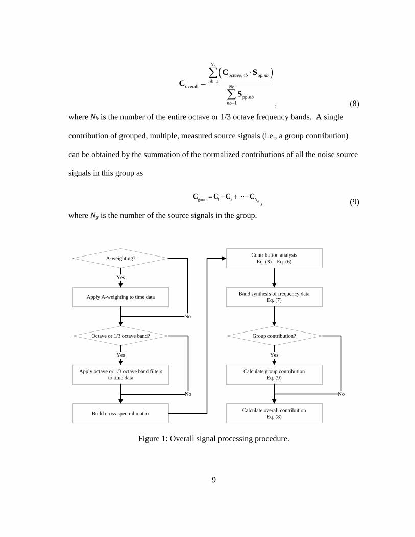
The overall signal processing procedure is shown in Figure 1. In this procedure,

it is assumed that time data is obtained from exterior and interior sensors connected to a

data acquisition system. If needed, the A-weighting is applied to the time data and

octave or 1/3 octave band pass filters are applied to the time signals to obtain the

contribution analysis results in octave or 1/3 octave bands. The cross-spectral matrices

are then built by applying the Fast Fourier Transformation (FFT) to the time-windowed

data and by averaging the spectra linearly. The contribution of each source to each

receiver is obtained from Eqs. (3) to (6) and the frequency data in each octave or 1/3

octave band is obtained by using the linear band summation in Eq. (7). The overall

contribution can be calculated by using Eq. (8).

11

3. EXPERIMENT WITH TWO SPEAKERS*

3.1 Experimental Setup

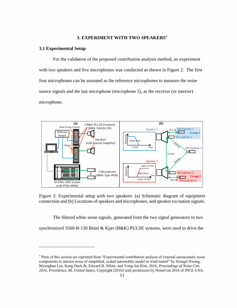
For the validation of the proposed contribution analysis method, an experiment

with two speakers and five microphones was conducted as shown in Figure 2. The first

four microphones can be assumed as the reference microphones to measure the noise

source signals and the last microphone (microphone 5), as the receiver (or interior)

microphone.

1.0 m

0.2 m

0.2 m

Microphone 2Speaker 1

Speaker 2

Freq.

Freq.

Mag

nit

ud

e

White Noise

Mag

nit

ud

e

White Noise

3.2 kHz

Microphone 1

Center: 10 kHz

Span: 6.4 kHz

(b)2 B&K PULSE Frontends

(B&K 3560-B-130)Multi Frame Control

Output

NI PXIe-1082 System

(with PXIe-4496s)

5 Microphones

(B&K Type 4958)

Speakers

(with Internal Amplifier)

(a)

Ethernet

Switch

Microphone 4

Microphone 5

Microphone 3

Group 1

Group 2

Figure 2: Experimental setup with two speakers: (a) Schematic diagram of equipment

connection and (b) Locations of speakers and microphones, and speaker excitation signals.

The filtered white noise signals, generated from the two signal generators in two

synchronized 3560-B-130 Brüel & Kjær (B&K) PULSE systems, were used to drive the





12

two speakers independently. The first excitation signal to drive speaker 1 is a low-pass-

filtered, white noise with the cut-off frequency of 3.2 kHz. The other excitation signal

for speaker 2 is a band-pass-filtered, white noise with the center frequency of 10 kHz

and the frequency span of 6.4 kHz.

The acoustic pressure signals were measured by connecting the microphones to a

National Instrument (NI) PXIe-1082 chassis with data acquisition modules of NI PXIe-

4496. An in-house NI LabVIEW code was built and used to acquire the microphone

time data at a sampling rate of 20 kHz for 120 seconds. The acquired time data was

processed by using an in-house MATLAB code to obtain the contributions of the

reference microphone signals to the receiver microphone signal.

3.2 Results and Discussion

Figure 3 shows the contribution analysis results of the experiment with the two

speakers. The normalized contributions, in Eq. (6), of the reference microphone signals

to the receiver microphone signal are presented in Figure 3(a). The total contribution

obtained by adding all the four normalized contributions at each frequency represents the

multiple coherence function in percent: i.e., the total contribution divided by 100

represents the multiple coherence function in the range of 0 to 1. The multiple

coherence function between the signals of the receiver microphone (i.e., microphone 5)

and the reference microphones (i.e., microphones 1 to 4) in the entire frequency range is

mostly higher than 0.8. This indicates that the contribution of the reference microphone

signal to the receiver microphone signal in this frequency range is dominant, resulting in

meaningful contribution data.

13

(a) (b)

(d)(c)

Figure 3: Contribution results with two speaker data: (a) Contribution in percent, (b)

Group contribution in percent, (c) Contribution in dB, and (d) Contribution in 1/3 octave

dBA.

The contribution analysis results in Figure 3(a) indicate that the microphone 1

and 2 signals are dominantly contributing to the auto-spectrum of microphone 5 in the

low frequency range up to 3.2 kHz. In the high frequency range of 6.8 kHz to 10 kHz,

the microphone 3 and 4 signals are most influential to the auto-spectrum of microphone

5.

The group contribution results calculated by using Eq. (9) are shown in Figure

3(b). Group 1 was including the acoustic pressure signals of microphones 1 and 2

placed in front of speaker 1 as shown in Figure 2(b), and the signals of microphones 3

14

and 4 located closer to speaker 2 were grouped as group 2. In the low frequency range,

up to 3.2 kHz, mainly excited by speaker 1, group 1 is dominant in the contribution

results, and in the high frequency range, above 6.8 kHz, dominantly excited by speaker

2, group 2 is significant.

The linearly scaled contribution in dB, introduced for the convenience to

interpret the contribution analysis results, is shown in Figure 3(c). This contribution is

calculated by linearly combining the contribution results in percent and the auto-

spectrum of the receiver microphone. For example, 42 % contribution of 90 dB at 100

Hz in Figure 3(c) is represented as 37.8 dB that is obtained by multiplying 0.42 and 90

dB. The gray colored contribution labeled as “Others” in Figure 3(c) and Figure 3(d)

represents a contribution of other sound sources (e.g., background noise) that are not

measured with the reference microphones.

In Figure 3(c), the total contribution obtained by linearly adding all the five

contributions (i.e., the four reference microphone contributions and the "other"

contribution) in dB represents the auto-spectrum of the receiver microphone signal. In

the low frequency range up to 3.2 kHz, the auto-spectra of microphones 1 and 2 are

approximately 10 to 30 dB higher than the others, since these two microphones are

placed closer to speaker 1 than the others. In the high frequency range of 6 kHz to 10

kHz, the auto-spectra of microphones 3 and 4 are approximately 10 to 40 dB higher than

the others due to their proximity to speaker 2. Finally, the contributions in 1/3 octave

bands are shown in Figure 3(d).

15

Figure 4 shows the comparison of the SVD- and CD-based contributions between

by using SVD shown in Figure 4 (a) and by using CD shown in Figure 4 (b). The SVD

based contribution is hard to identify the measured channels although it looks very

similar with CD based contribution s of microphones 1 and 2 at the low frequencies can

be associated with the sound radiation from speaker 1 since microphones 1 and 2 are

placed close to speaker 1 and the contribution results at the high frequencies can be

related to the sound radiation from speaker 2.

(a) (b)

Figure 4: Contribution results with two speaker data: (a) SVD-based contribution, (b) CD-

based contribution.

16

4. EXPERIMENT WITH SIMPLIFIED, SCALED AUTOMOBILE MODEL*

4.1 Design Overview

Side Mirror

Bottom Plate

Front Window

Side PlateSide Window

Rear Plate

Rain GuttersFillet Plate

Front Plate

FilletTop Plate

Figure 5: Simplified, scaled automobile model.

A simplified automobile model was designed based on the Hyundai Simplified

Model (HSM) [24] and scaled down to fit the test section of the Klebanoff-Saric Wind

Tunnel (KSWT) at Texas A&M University as shown in Figure 5. This simplified,





17

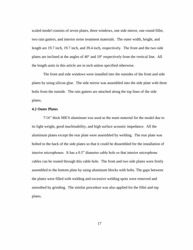
scaled model consists of seven plates, three windows, one side mirror, one round fillet,

two rain gutters, and interior noise treatment materials. The outer width, height, and

length are 19.7 inch, 19.7 inch, and 39.4 inch, respectively. The front and the two side

plates are inclined at the angles of 40° and 10° respectively from the vertical line. All

the length units in this article are in inch unless specified otherwise.

The front and side windows were installed into the outsides of the front and side

plates by using silicon glue. The side mirror was assembled into the side plate with three

bolts from the outside. The rain gutters are attached along the top lines of the side

plates.

4.2 Outer Plates

7/16” thick MIC6 aluminum was used as the main material for the model due to

its light weight, good machinability, and high surface acoustic impedance. All the

aluminum plates except the rear plate were assembled by welding. The rear plate was

bolted to the back of the side plates so that it could be dissembled for the installation of

interior microphones. It has a 0.5” diameter cable hole so that interior microphone

cables can be routed through this cable hole. The front and two side plates were firstly

assembled to the bottom plate by using aluminum blocks with bolts. The gaps between

the plates were filled with welding and excessive welding spots were removed and

smoothed by grinding. The similar procedure was also applied for the fillet and top

plates.

18

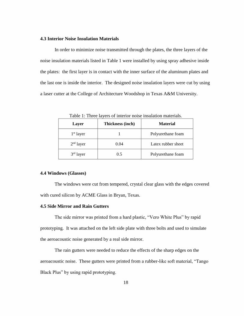
4.3 Interior Noise Insulation Materials

In order to minimize noise transmitted through the plates, the three layers of the

noise insulation materials listed in Table 1 were installed by using spray adhesive inside

the plates: the first layer is in contact with the inner surface of the aluminum plates and

the last one is inside the interior. The designed noise insulation layers were cut by using

a laser cutter at the College of Architecture Woodshop in Texas A&M University.

Table 1: Three layers of interior noise insulation materials.

Layer Thickness (inch) Material

1st layer 1 Polyurethane foam

2nd layer 0.04 Latex rubber sheet

3rd layer 0.5 Polyurethane foam

4.4 Windows (Glasses)

The windows were cut from tempered, crystal clear glass with the edges covered

with cured silicon by ACME Glass in Bryan, Texas.

4.5 Side Mirror and Rain Gutters

The side mirror was printed from a hard plastic, “Vero White Plus” by rapid

prototyping. It was attached on the left side plate with three bolts and used to simulate

the aeroacoustic noise generated by a real side mirror.

The rain gutters were needed to reduce the effects of the sharp edges on the

aeroacoustic noise. These gutters were printed from a rubber-like soft material, “Tango

Black Plus” by using rapid prototyping.

19

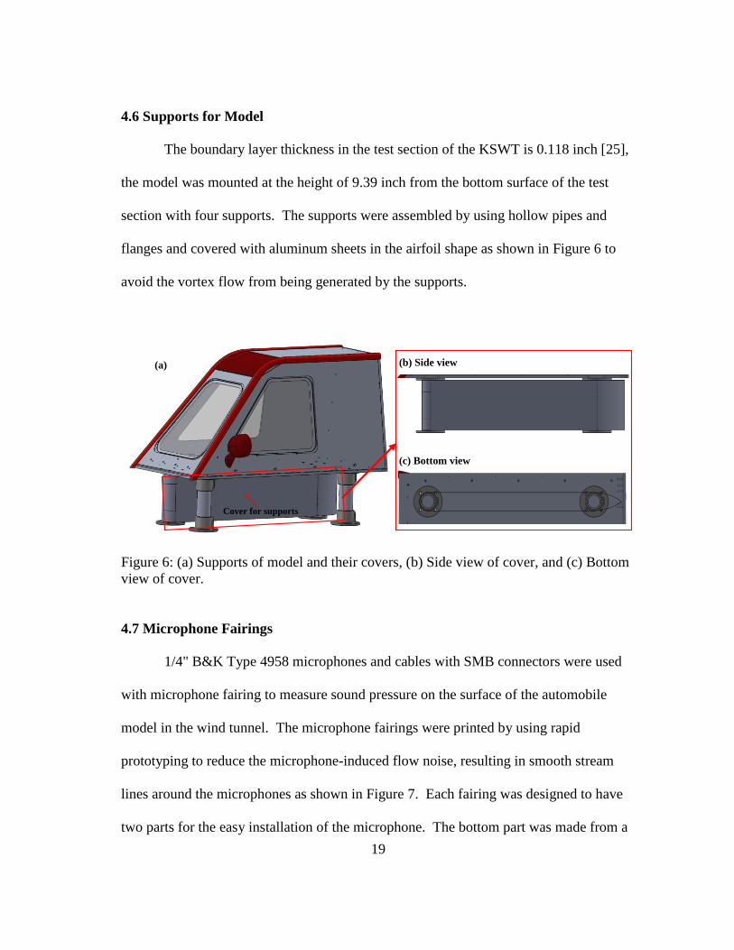
4.6 Supports for Model

The boundary layer thickness in the test section of the KSWT is 0.118 inch [25],

the model was mounted at the height of 9.39 inch from the bottom surface of the test

section with four supports. The supports were assembled by using hollow pipes and

flanges and covered with aluminum sheets in the airfoil shape as shown in Figure 6 to

avoid the vortex flow from being generated by the supports.

Cover for supports

(a) (b) Side view

(c) Bottom view

Figure 6: (a) Supports of model and their covers, (b) Side view of cover, and (c) Bottom

view of cover.

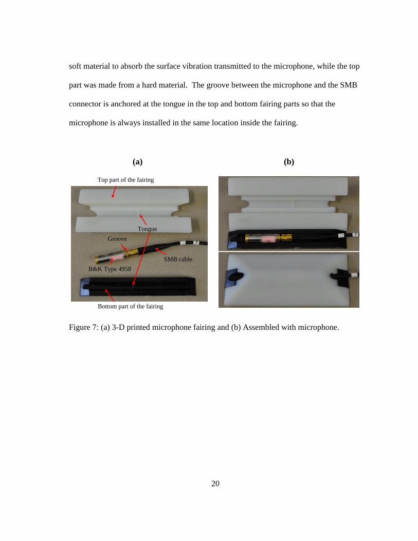
4.7 Microphone Fairings

1/4" B&K Type 4958 microphones and cables with SMB connectors were used

with microphone fairing to measure sound pressure on the surface of the automobile

model in the wind tunnel. The microphone fairings were printed by using rapid

prototyping to reduce the microphone-induced flow noise, resulting in smooth stream

lines around the microphones as shown in Figure 7. Each fairing was designed to have

two parts for the easy installation of the microphone. The bottom part was made from a

20

soft material to absorb the surface vibration transmitted to the microphone, while the top

part was made from a hard material. The groove between the microphone and the SMB

connector is anchored at the tongue in the top and bottom fairing parts so that the

microphone is always installed in the same location inside the fairing.

Tongue

Top part of the fairing

Bottom part of the fairing

(a) (b)

SMB cable

Groove

B&K Type 4958

Figure 7: (a) 3-D printed microphone fairing and (b) Assembled with microphone.

21

5. WIND TUNNEL TEST AND RESULTS*

5.1 Klebanoff-Saric Wind Tunnel

The automobile model was tested at the Klebanoff-Saric Wind Tunnel (KSWT)

(see Table 2) that has acoustically treated inner walls so that its background noise level

is relatively low. The dimensions of the automobile model were decided by the KSWT

test section dimensions. The number of the KSWT fan blades is 9.

Table 2: Information on Klebanoff-Saric Wind Tunnel (KSWT) [26] at Texas A&M

University.

Item Value

Test Section Dimensions (H×W×L) 1.4×1.4×4.9 m (4.5×4.5×16 ft)

Maximum Wind Speed 20 m/s (72 km/h or 44.74 miles/h)

Acoustically Treated Inner Walls Yes

5.2 Experimental Setup for Wind Tunnel Test

The automobile model was installed in the test section of the KSWT. The

bottom flanges of the supports were fixed with bolts to the floor of the test section and

the covers of the supports shown in Figure 6 were filled with noise insulation foam and

wrapped by using duct tape. Any gaps (or steps) on the surfaces of the automobile





22

model, the microphone fairings, and the microphone cables were sealed with vinyl

insulation tape to have smooth airflow.

Mic. 1

Mic. 2

Mic. 3

Mic. 6

Mic. 7

Mic. 8

Mic. 11

(Front Window)

Mic. 15

(Interior)

Mic. 4

Mic. 5

Mic. 9

Mic. 10

Mic. 12

(Top)

Mic. 13

(Bottom)

Mic 14

(Back)

LEFT RIGHT

(b)(a)

Mic. 1

(Left: Front of Side Mirror)

Mic. 2

(Left: Rear of Side Mirror)

Mic. 3

(Left: Middle of Gutter)

Mic. 4

(Left: Top of Gutter)

Mic. 5

(Left: Side Rear)

Mic. 12

(Top)

Mic 14

(Back)

Mic. 13

(Bottom)

Mic. 11

(Front Window)

Figure 8: Microphone locations in automobile model: (a) Left side view and (b) Top view.

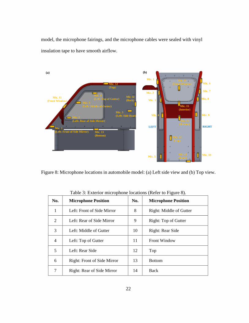
Table 3: Exterior microphone locations (Refer to Figure 8).

No. Microphone Position No. Microphone Position

1 Left: Front of Side Mirror 8 Right: Middle of Gutter

2 Left: Rear of Side Mirror 9 Right: Top of Gutter

3 Left: Middle of Gutter 10 Right: Rear Side

4 Left: Top of Gutter 11 Front Window

5 Left: Rear Side 12 Top

6 Right: Front of Side Mirror 13 Bottom

7 Right: Rear of Side Mirror 14 Back

23

For the acoustic pressure measurement, 14 microphones with the fairings were

placed on the outer surface of the automobile model and 1 microphone was located

inside the model as shown in Figure 8. These 15 B&K Type 4958 microphones were

calibrated with the sound calibrator, B&K Sound Calibrator Type 4231 (94 dB @ 1 kHz)

in the NI MAX software as in the two speaker experiment. The in-house NI LabVIEW

code was again used to acquire the microphone time data at a sampling rate of 20 kHz

for 120 seconds.

5.3 Wind Tunnel Test

Table 4: Configurations of wind tunnel test and interior acoustic resonance test.

Airflow Speed With Interior

Noise Treatment

Without Interior

Noise Treatment

0 m/s

(no flow) -

Test Configuration 5

(Identification of interior

resonances with one speaker

and one microphone)

15 m/s Test Configuration 1 Test Configuration 3

24 m/s Test Configuration 2 Test Configuration 4

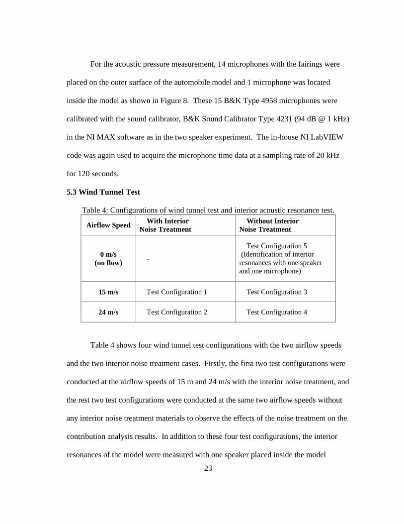
Table 4 shows four wind tunnel test configurations with the two airflow speeds

and the two interior noise treatment cases. Firstly, the first two test configurations were

conducted at the airflow speeds of 15 m and 24 m/s with the interior noise treatment, and

the rest two test configurations were conducted at the same two airflow speeds without

any interior noise treatment materials to observe the effects of the noise treatment on the

contribution analysis results. In addition to these four test configurations, the interior

resonances of the model were measured with one speaker placed inside the model

24

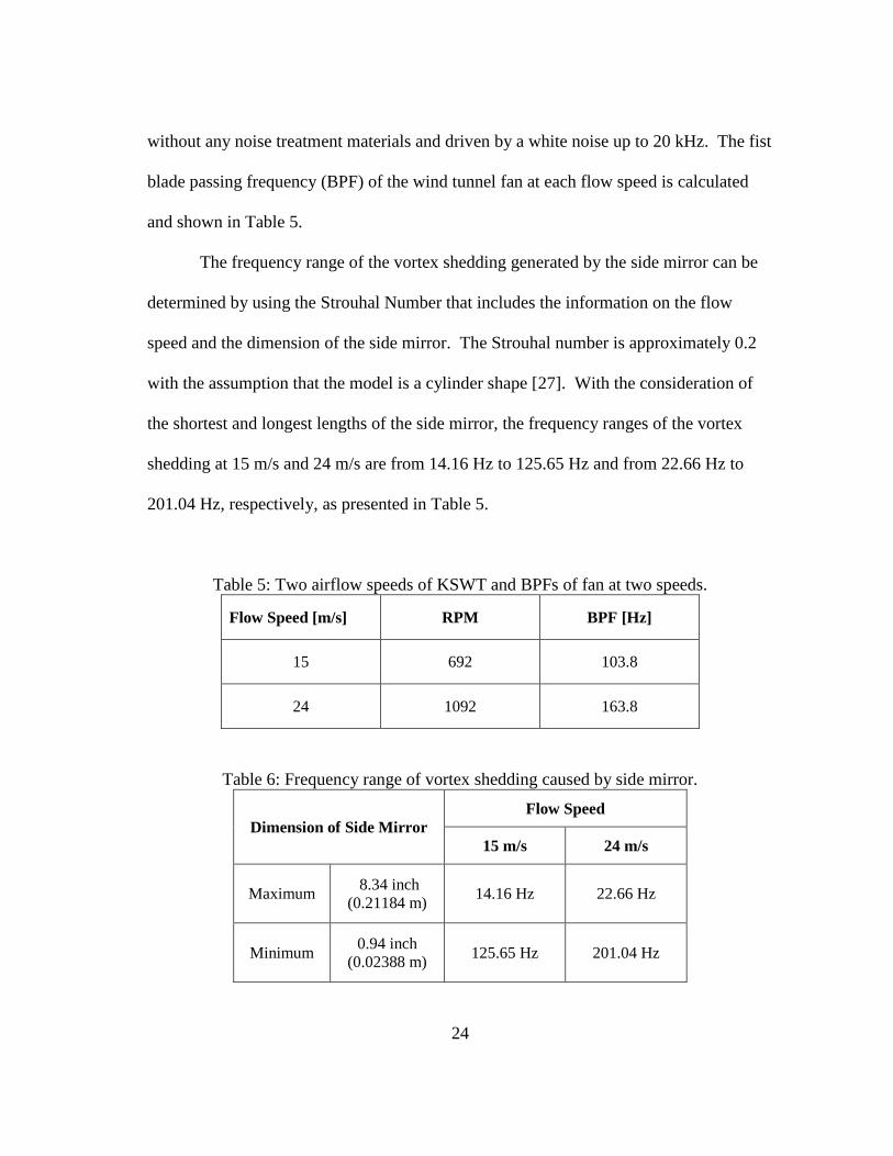
without any noise treatment materials and driven by a white noise up to 20 kHz. The fist

blade passing frequency (BPF) of the wind tunnel fan at each flow speed is calculated

and shown in Table 5.

The frequency range of the vortex shedding generated by the side mirror can be

determined by using the Strouhal Number that includes the information on the flow

speed and the dimension of the side mirror. The Strouhal number is approximately 0.2

with the assumption that the model is a cylinder shape [27]. With the consideration of

the shortest and longest lengths of the side mirror, the frequency ranges of the vortex

shedding at 15 m/s and 24 m/s are from 14.16 Hz to 125.65 Hz and from 22.66 Hz to

201.04 Hz, respectively, as presented in Table 5.

Table 5: Two airflow speeds of KSWT and BPFs of fan at two speeds.

Flow Speed [m/s] RPM BPF [Hz]

15 692 103.8

24 1092 163.8

Table 6: Frequency range of vortex shedding caused by side mirror.

Dimension of Side Mirror

Flow Speed

15 m/s 24 m/s

Maximum 8.34 inch

(0.21184 m) 14.16 Hz 22.66 Hz

Minimum 0.94 inch

(0.02388 m) 125.65 Hz 201.04 Hz

25

5.4 Test Results and Discussion

Figure 9 shows the auto-spectra of the interior microphone and the multiple

coherence between the external and internal microphone signals for test configuration 4

at the wind speed of 24 m/s without the interior noise treatment. In the high frequency

region above 1 kHz, the multiple coherence is low (e.g., below 0.4), which indicates that

the exterior microphones are not capturing entire aeroacoustic noise sources. Thus, the

test results from Figure 10 are presented only in the frequency range below 1 kHz.

Figure 10 shows the comparison of the auto-spectra between the four test

configurations in Table 4. In Figure 10, the vertical yellow lines indicate the BPF and its

harmonics of the wind tunnel fan. With the interior noise treatment installed, the interior

noise level is approximately 70 dB lower than the exterior noise levels around 1 kHz.

Even when the noise treatment materials are removed, the interior noise level is still

approximately 40 dB lower than the exterior noise levels around 1 kHz. This large noise

reduction even without the interior noise treatment is caused by the 7/16-inch-thick

aluminum panels. They can cause the high sound transmission loss, significantly

reducing the transmitted noise from the exterior to the interior, in particular, at high

frequencies. In addition, the 24 m/s airflow cases show higher noise levels than the 15

m/s cases, thus having higher signal-to-noise ratio (SNR) than the 15 m/s cases.

Therefore, the only results for test configuration 4 at the airflow speed of 24 m/s without

the interior noise treatment, are presented below, in which the contribution of the

exterior aeroacoustic noise sources to the interior noise is more distinctly presented than

other test configurations due to the high SNR.

26

(a)

(b)

Figure 9: Wind tunnel test results at airflow speed of 24 m/s without interior noise

treatment in frequency range up to 4 kHz. (a) Auto-spectrum of interior microphone in

both wind tunnel test and interior acoustic resonance test and (b) Multiple coherence

between exterior and interior microphone signals in wind tunnel test.

Noise

Insulation

Flow

Speed

(a) (b)

(c) (d)

Figure 10: Comparison of auto-spectra measured by using exterior and interior

microphones in 4 test configurations. (a) 15 m/s with interior noise treatment, (b) 24 m/s

with interior noise treatment, (c) 15 m/s without interior noise treatment, and (d) 24 m/s

without interior noise treatment.

27

(a)

(b)

(c)

Figure 11: Results of wind tunnel test at flow speed of 24 m/s without interior noise

treatment and interior resonance test without both airflow and interior noise treatment. (a)

Auto-spectrum of interior microphone, (b) Multiple coherence between exterior and

interior microphone signals, and (c) Interior auto-spectrum decomposed by using

normalized contribution.

Figure 11 shows the contribution analysis results along with the interior auto-

spectra and the multiple coherence up to 1k Hz for test configuration 4. Figure 12 and

Figure 13 show the zoomed views of Figure 11 at selected interior noise peak

frequencies and Table 7 and Table 8 presents the first three highest contributions of the

exterior noise sources to the interior noise at the selected frequencies. Table 3 presents

the exterior microphone numbers and their locations used in Table 7 and Table 8.

The frequency of 164 Hz (Figure 12(a)) coincides with the BPF, the one of the

interior resonance frequencies, and the vortex shedding frequency caused by the side

mirror (see Table 6). As shown in Table 7 and Table 8, the first two highest

28

contributions are from the front of the left side mirror and the left rear side at the

normalized contributions of 35.92 % and 23.01 %, respectively, indicating that the

vortex shedding generated from the left side mirror is dominantly contributing to the

interior noise at 164 Hz. Most of the selected interior noise peaks (e.g., 205 Hz, 669 Hz,

803 Hz, 878 Hz, and 965 Hz) in Figure 12 and Figure 13 are mainly generated from the

interior resonances. Thus, the multiple coherence is low at these interior resonance

frequencies. At these frequencies, unless there are other causes to generate the interior

noise peaks, all the aeroacoustic sources contribute insignificantly with the maximum

single source contribution of approximately 15 % or below. Although the peak at 364

Hz (Figure 12(c)) seems to be generated by the interior resonance, the multiple

coherence is approximately 0.5 indicates that the vortex shedding at the back (13.04 %)

and the airflow on the front window (10.99 %) are also contributing meaningfully to the

interior noise. The peaks at 498 Hz (Figure 12(d)) and 736 Hz (Figure 13(a)) are also

generated by the interior resonances, although the aeroacoustic noise sources at the front

window, the left gutter, and the back are largely contributing to the interior noise. The

5th harmonics of the BPF is almost coincident with the interior noise peak at 817 Hz,

indicating that the noise generated by the wind tunnel fan is dominant. At this

frequency, the front window has the highest contributions of 34.25 % as shown in Table

8.

29

(a) (b) (c) (d) (e)

Figure 12: Zoomed contribution results: (a) 164 Hz, (b) 205 Hz, (c) 364 Hz, (d) 498 Hz,

and (e) 669 Hz.


Figure 12.

Frequency [Hz] 164 205 364 498 669

1st Microphone No. 1 8 14 11 11

Contribution [%] 35.92 5.5 13.04 17.53 7.34

2nd Microphone No. 5 11 11 14 3

Contribution [%] 23.01 4.29 10.99 14.67 4.33

3rd Microphone No. 11 7 7 12 12

Contribution [%] 14.5 2.59 6.14 4.01 3.97

30

(a) (b) (c) (d) (e)

Figure 13: Zoomed contribution results: (a) 736 Hz, (b) 803 Hz, (c) 817 Hz, (d) 878 Hz,

and (e) 965 Hz.


Figure 13.

Frequency [Hz] 736 803 817 878 965

1st Microphone No. 11 3 11 14 14

Contribution [%] 13.17 14.5 34.25 6.18 6.55

2nd Microphone No. 5 11 11 14 3

Contribution [%] 12.59 3.62 3.51 5.34 4.52

3rd Microphone No. 11 7 7 12 12

Contribution [%] 2.77 1.86 2.27 1.84 3.88

31

6. EXPERIMENT WITH AUTOMOBILE AND RESULTS

6.1 Experimental Setup for Automobile Test

Trunk

Exterior

(a) (b)

ANL Fuse

12 V BatteryPower Inverter

NI PXIe-1082

(with 5 PXIe-4496s)

Interior

DC

Power

AC

Power

12V

Battery

Power

Inverter

NI PXIe-1082

(with PXIe-4496s)

Laptop

Compter4 Microphones

64

Microphones

Analog Signals

Figure 14: Experimental setup with automobile: (a) Schematic of equipment connection

and (b) Equipment inside automobile’s trunk.

FRONT DRIVER SIDEFRONT PASSENGER SIDE REAR DRIVER SIDE REAR PASSENGER SIDE

LEFT SIDE

RIGHT SIDE

ENGINE64 ENGINE

INTERIOR

1

2

4

5

3

6

11

10

12

13

14

15

9

8

17

16

18

19

20

21

22

23

24

25

26

7

27

28

29

30

31

32

33

35

34

37

36

31

40

39

38

42

43

44

46

45

48

49

50

51

52

47

33

31

32

28

27

24

26

25

5

6

7

1

2

50

52

51

CENTER

EXTERIOR}

5455 53

56

57

58

59

63

62

61

60

6566 67 68

Figure 15: Microphone installation locations. Refer to Table 9 for the description of the

microphone locations.

32

An automobile (Hyundai Sonata) was instrumented and tested on a road at the

two cruising speeds of 65 mph and 80 mph. Figure 14(a) shows the schematic diagram

of the instrumentation for this experiment. A 12V battery and a power inverter were

used to power a NI PXIe-1082 chassis with five NI PXIe-4496 data acquisition modules.

The measurement equiment was placed in the trunk shown in Figure 14(b) to avoid the

fan noise, of the NI PXIe-1082 chassis, that contaminated inteior microphone signals.

The in-house NI LabVIEW code from the previous two speaker experiment was reused

to acquire the time data of both 64 exterior and 4 interior microphones at a sampling rate

of 20 kHz for 30 seconds.

32

HOOD

WIND SHIELD REAR WINDOW

TRUNK

WIPER

ENGINE

1

2

3

4

5

7

8

9

11

12

13

6 10

14

15

16

17

19

18

20

21

22

23

24

26

25FRONT WINDOW (BTM)

FRONTFRONT FENDER

REAR WINDOW (BTM)

A-PILLAR

SIDE MIRRORFRONT DOOR

HANDLE

REAR DOOR

HANDLE

REAR DOORREAR FENDER

C-PILLAR

FRONT WINDOW (TOP)REAR WINDOW (TOP)

27

28

31

3029

LEFT SIDE

RIGHT SIDE

CENTER

Figure 16: Locations of grouped microphones. Refer to Table 10 for the description of

the microphone groups.

33

Table 9: List of noise source microphone locations (Refer to Figure 15).

No. Position No. Position

1 Left of front bumper 33 Right wind shield

2 Bottom of left headlamp 34 Lower front of front right window

3 Front of left A-pillar 35 Upper front of front right window

4 Rear of front left fender 36 Lower middle of front right window

5 Front of left side mirror 37 Upper middle of front right window

6 Bottom of left side mirror 38 Front of right door handle

7 Left wind shield 39 Lower rear of front right window

8 Lower front of front left window 40 Middle rear of front right window

9 Upper front of front left window 41 Upper rear of front right window

10 Lower middle of front left window 42 Middle front of rear right door

11 Upper middle of front left window 43 Lower front of rear right window

12 Front of left door handle 44 Upper front of rear right window

13 Lower rear of front left window 45 Lower middle of rear right window

14 Middle rear of front left window 46 Upper middle of rear right window

15 Upper rear of front left window 47 Lower rear of rear right window

16 Middle front of rear left door 48 Upper rear of rear right window

17 Lower front of rear left window 49 Rear of right door handle

18 Upper front of rear left window 50 Right C-pillar

19 Lower middle of rear left window 51 Rear of rear right fender

20 Upper middle of rear left window 52 Right of trunk door

21 Lower rear of rear left window 53 Front middle hood

22 Upper rear of rear left window 54 Front left hood

23 Rear of left door handle 55 Front right hood

24 Left C-pillar 56 Rear middle hood

25 Rear of rear left fender 57 Front middle wind shield

26 Left of trunk door 58 Middle of wind shield

27 Right of front bumper 59 Front middle ceiling

28 Bottom of right headlamp 60 Rear middle ceiling

29 Front of right A-pillar 61 Middle of rear window

30 Rear of front right fender 62 Upper middle of trunk door

31 Front of right side mirror 63 Rear middle of trunk door

32 Bottom of right side mirror 64 Engine

34

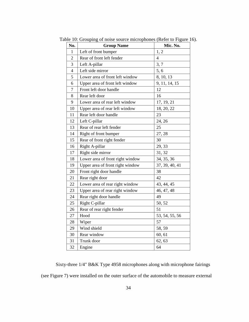
Table 10: Grouping of noise source microphones (Refer to Figure 16).

No. Group Name Mic. No.

1 Left of front bumper 1, 2

2 Rear of front left fender 4

3 Left A-pillar 3, 7

4 Left side mirror 5, 6

5 Lower area of front left window 8, 10, 13

6 Upper area of front left window 9, 11, 14, 15

7 Front left door handle 12

8 Rear left door 16

9 Lower area of rear left window 17, 19, 21

10 Upper area of rear left window 18, 20, 22

11 Rear left door handle 23

12 Left C-pillar 24, 26

13 Rear of rear left fender 25

14 Right of front bumper 27, 28

15 Rear of front right fender 30

16 Right A-pillar 29, 33

17 Right side mirror 31, 32

18 Lower area of front right window 34, 35, 36

19 Upper area of front right window 37, 39, 40, 41

20 Front right door handle 38

21 Rear right door 42

22 Lower area of rear right window 43, 44, 45

23 Upper area of rear right window 46, 47, 48

24 Rear right door handle 49

25 Right C-pillar 50, 52

26 Rear of rear right fender 51

27 Hood 53, 54, 55, 56

28 Wiper 57

29 Wind shield 58, 59

30 Rear window 60, 61

31 Trunk door 62, 63

32 Engine 64

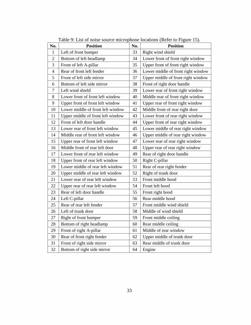
Sixty-three 1/4" B&K Type 4958 microphones along with microphone fairings

(see Figure 7) were installed on the outer surface of the automobile to measure external

35

aeroacoustic noise signals. Here, the microphone fairings were used to reduce the

microphone-induced flow noise, resulting in smooth stream lines around the microphone

and fairing assemblies. One 1/4" B&K Type 4958 microphone was also located close to

the engine in the engine room to acquire the engine noise data. Exterior microphone

cables were covered by using plastic insulation tapes to reduce the cable-induced flow

noise. Four 1/2" B&K Type 4189-A-021 microphones were placed on the window-side

head rests at the four seat positions to measure the interior noise signals. Figure 15 and

Table 9 show the channel numbers of all the microphones and their locations. As shown

in Figure 15, 26 microphones were installed at each side of the automobile, 11

microphones on the other exterior surfaces except the underbody of the automobile, and

1 microphone inside the engine room. Figure 16 and Table 10 show 32 microphone

groups to effectively observe the contributions of the areas covered by the grouped

microphones to the interior noise.

6.2 Test Results and Discussion

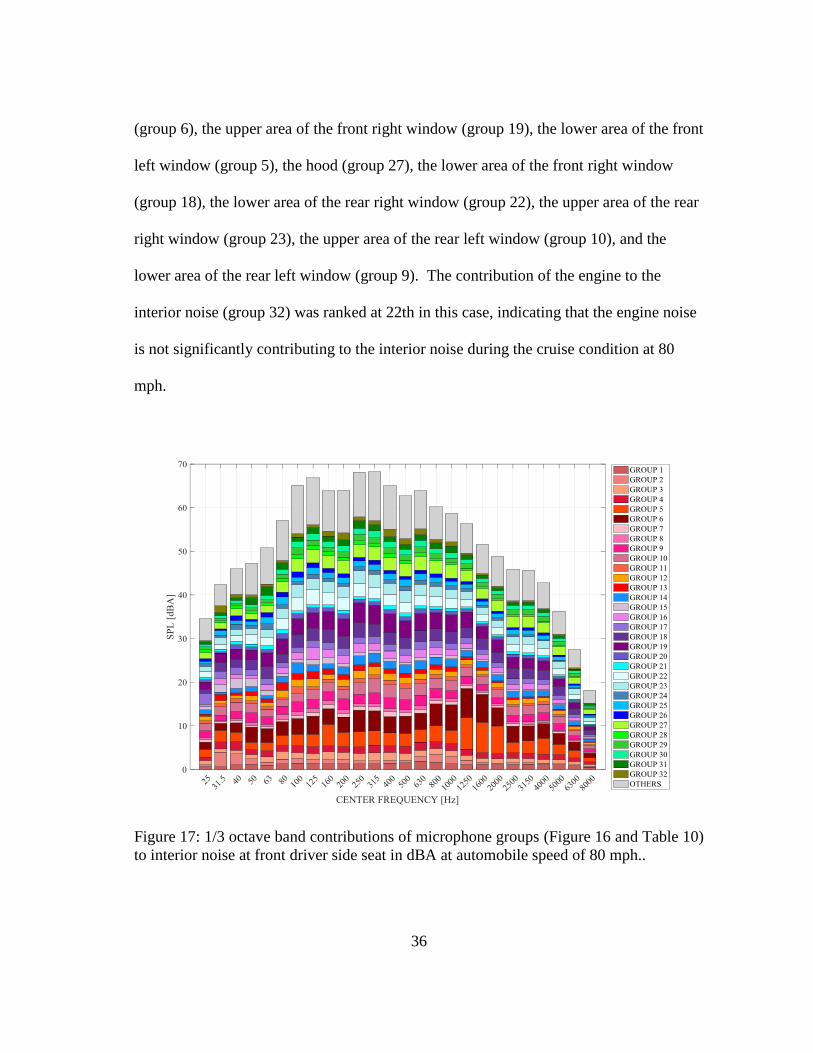
Figure 17 shows the 1/3 octave band contributions, in dBA, of the microphone

groups to the interior noise at the front driver side seat and the automobile speed of 80

mph. At first glance, it can be observed that the contribution of the front left window

(groups 5 and 6) closed to the front driver side seat seems to be high compared to other

groups, although it is difficult to be quantitatively compared to the other contributions.

Therefore, the overall contributions of all the microphone groups were presented in

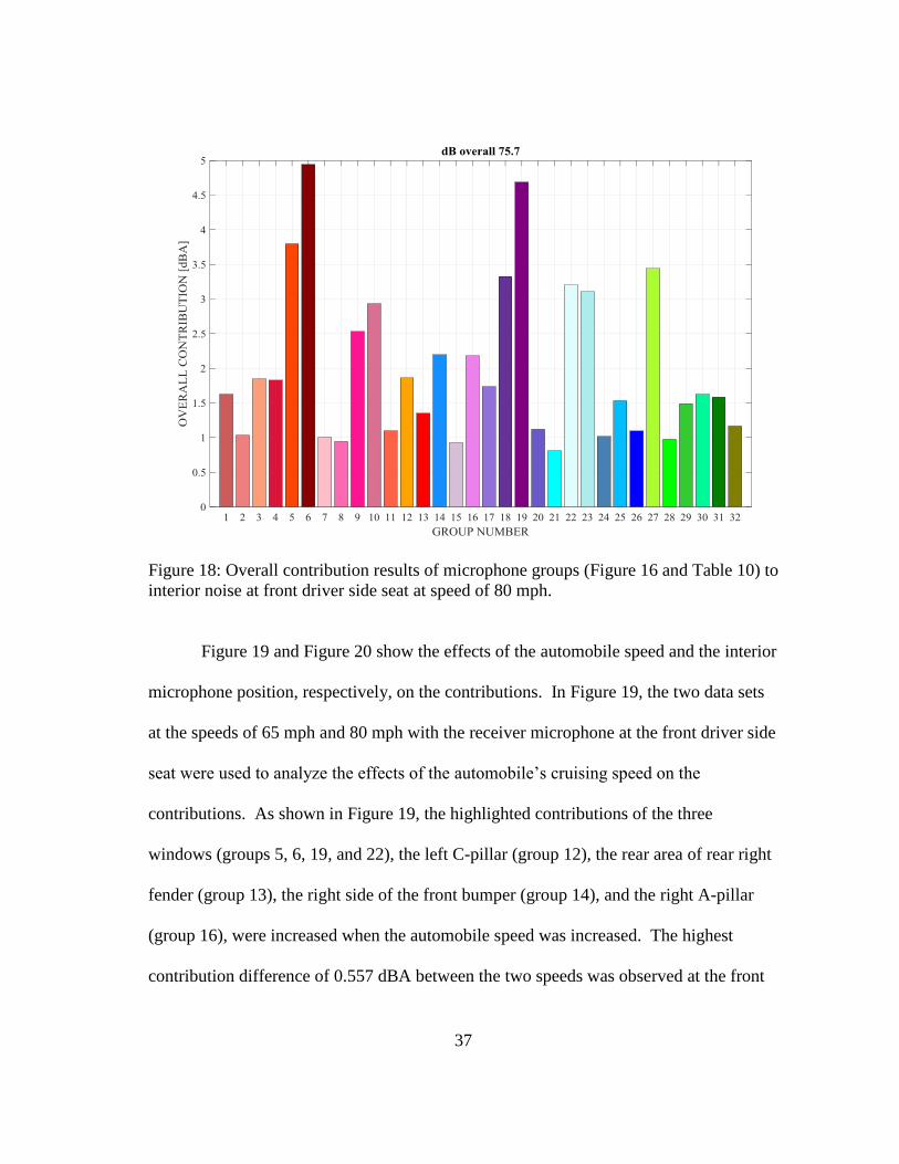
Figure 18. The first nine highest contributions were observed at the four windows and

the hood: i.e., from the highest to the lowest, the upper area of the front left window

36

(group 6), the upper area of the front right window (group 19), the lower area of the front

left window (group 5), the hood (group 27), the lower area of the front right window

(group 18), the lower area of the rear right window (group 22), the upper area of the rear

right window (group 23), the upper area of the rear left window (group 10), and the

lower area of the rear left window (group 9). The contribution of the engine to the

interior noise (group 32) was ranked at 22th in this case, indicating that the engine noise

is not significantly contributing to the interior noise during the cruise condition at 80

mph.

Figure 17: 1/3 octave band contributions of microphone groups (Figure 16 and Table 10)

to interior noise at front driver side seat in dBA at automobile speed of 80 mph..

37

Figure 18: Overall contribution results of microphone groups (Figure 16 and Table 10) to

interior noise at front driver side seat at speed of 80 mph.

Figure 19 and Figure 20 show the effects of the automobile speed and the interior

microphone position, respectively, on the contributions. In Figure 19, the two data sets

at the speeds of 65 mph and 80 mph with the receiver microphone at the front driver side

seat were used to analyze the effects of the automobile’s cruising speed on the

contributions. As shown in Figure 19, the highlighted contributions of the three

windows (groups 5, 6, 19, and 22), the left C-pillar (group 12), the rear area of rear right

fender (group 13), the right side of the front bumper (group 14), and the right A-pillar

(group 16), were increased when the automobile speed was increased. The highest

contribution difference of 0.557 dBA between the two speeds was observed at the front

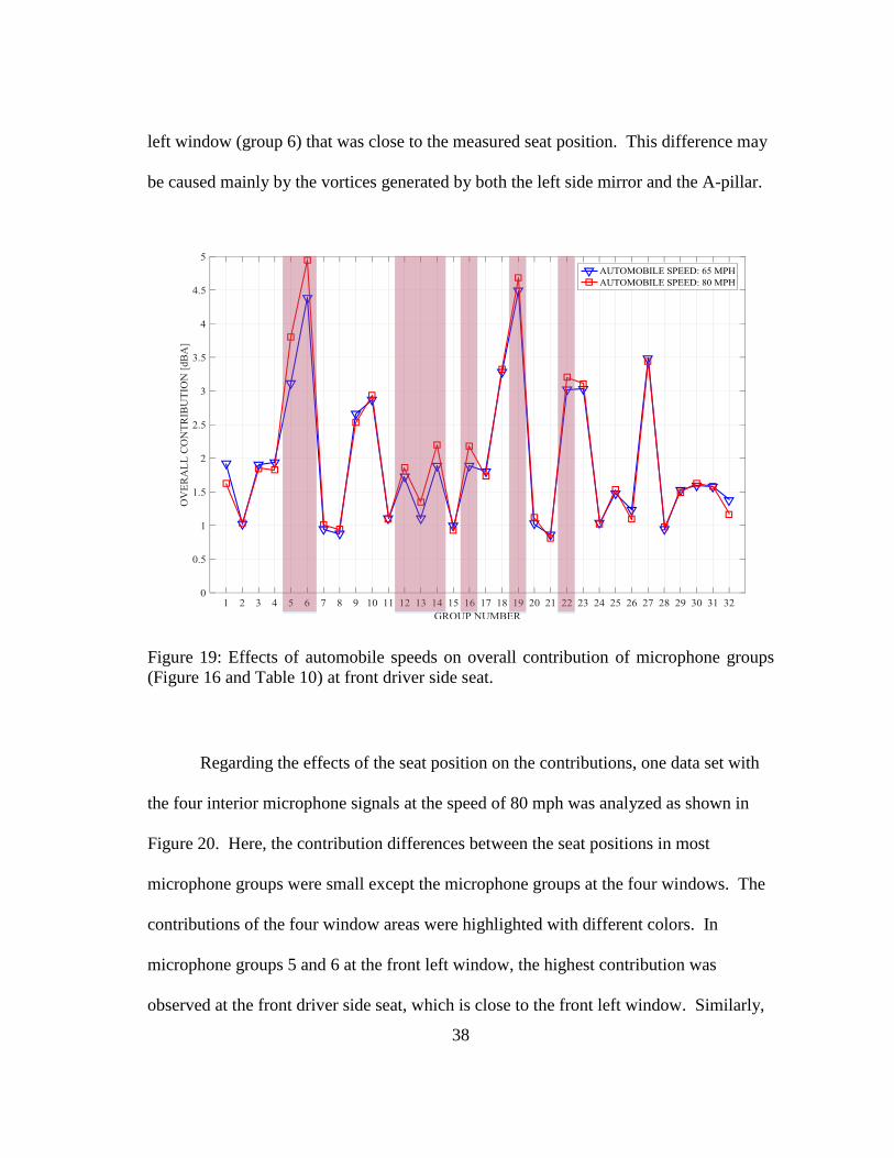
38

left window (group 6) that was close to the measured seat position. This difference may

be caused mainly by the vortices generated by both the left side mirror and the A-pillar.

Figure 19: Effects of automobile speeds on overall contribution of microphone groups

(Figure 16 and Table 10) at front driver side seat.

Regarding the effects of the seat position on the contributions, one data set with

the four interior microphone signals at the speed of 80 mph was analyzed as shown in

Figure 20. Here, the contribution differences between the seat positions in most

microphone groups were small except the microphone groups at the four windows. The

contributions of the four window areas were highlighted with different colors. In

microphone groups 5 and 6 at the front left window, the highest contribution was

observed at the front driver side seat, which is close to the front left window. Similarly,

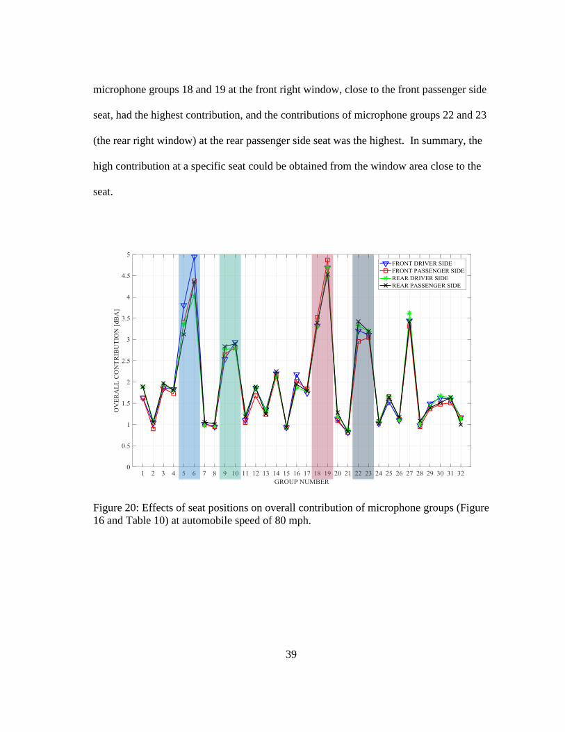
39

microphone groups 18 and 19 at the front right window, close to the front passenger side

seat, had the highest contribution, and the contributions of microphone groups 22 and 23

(the rear right window) at the rear passenger side seat was the highest. In summary, the

high contribution at a specific seat could be obtained from the window area close to the

seat.

Figure 20: Effects of seat positions on overall contribution of microphone groups (Figure

16 and Table 10) at automobile speed of 80 mph.

40

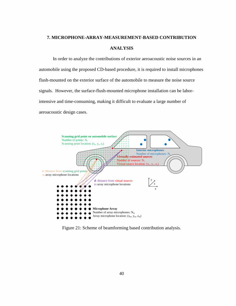
7. MICROPHONE-ARRAY-MEASUREMENT-BASED CONTRIBUTION

ANALYSIS

In order to analyze the contributions of exterior aeroacoustic noise sources in an

automobile using the proposed CD-based procedure, it is required to install microphones

flush-mounted on the exterior surface of the automobile to measure the noise source

signals. However, the surface-flush-mounted microphone installation can be labor-

intensive and time-consuming, making it difficult to evaluate a large number of

aeroacoustic design cases.

Scanning grid point on automobile surface

Number of points: Ns

Scanning point location: (xs, ys, zs)

Microphone Array

Number of array microphones: Nm

Array microphone location: (xm, ym, zm)

r: distance from scanning grid points

to array microphone locations

d: distance from virtual sources

to array microphone locations

Virtually estimated sources

Number of sources: Nv

Virtual source location: (xv, yv, zv)

Interior microphones

Number of microphones: Ni

x

y

z

Figure 21: Scheme of beamforming based contribution analysis.

41

7.1 Identification of Source Locations Using Two Beamforming Methods

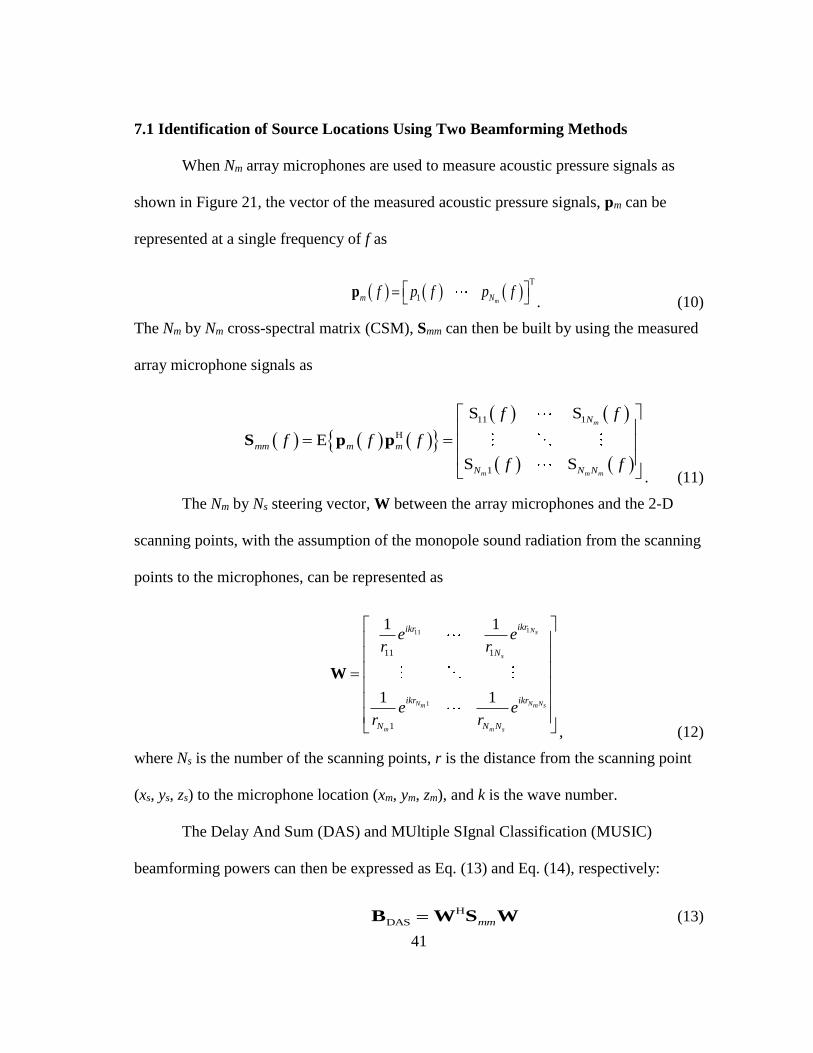
When Nm array microphones are used to measure acoustic pressure signals as

shown in Figure 21, the vector of the measured acoustic pressure signals, pm can be

represented at a single frequency of f as

T

1 mm Nf p f p f p. (10)

The Nm by Nm cross-spectral matrix (CSM), Smm can then be built by using the measured

array microphone signals as

11 1

H

1

S S

E

S S

m

m m m

N

mm m m

N N N

f f

f f f

f f

S p p

. (11)

The Nm by Ns steering vector, W between the array microphones and the 2-D

scanning points, with the assumption of the monopole sound radiation from the scanning

points to the microphones, can be represented as

111

1

11 1

1

1 1

1 1

Ns

s

N N Nm m s

m m s

ikrikr

N

ikr ikr

N N N

e er r

e er r

W

, (12)

where Ns is the number of the scanning points, r is the distance from the scanning point

(xs, ys, zs) to the microphone location (xm, ym, zm), and k is the wave number.

The Delay And Sum (DAS) and MUltiple SIgnal Classification (MUSIC)

beamforming powers can then be expressed as Eq. (13) and Eq. (14), respectively:

H

DAS mmB W S W (13)

42

MUSIC2

H

1

1M

i

i nd

B

W u

, (14)

where ui is the i-th column vector of the factorized unitary matrix U obtained by

applying the SVD to Smm (i.e., Smm = U∙Σ∙VH) and nd is the dimension of the signal

space. The virtual source locations can then be determined at the locations of the local

beamforming power maxima.

7.2 Reconstruction of Virtual Source Signals from Measured Array Signals

When the sound radiation characteristics from noise sources to the array

microphones are same as the monopoles, the acoustic pressure vector, pm measured by

using the array can be represented with the Nm by Nv propagator matrix, G between the

virtual source locations and the array microphone locations as

m p Gv, (15)

where v is the complex amplitude vector of the virtual sources and the propagator matrix

G is defined as

111

1

11 1

1

1 1

1 1

Nv

v

N N Nm m v

m m v

ikdikd

N

ikd ikd

N N N

e ed d

e ed d

G

, (16)

where Nv is the number of the virtual sources, d is the distance from the virtual source

(xv, yv, zv) to the microphone location (xm, ym, zm).

By substituting Eq. (15) into Eq. (11), Eq. (11) can be rewritten as

43

HEmm vv

S Gvv G GS G, (17)

where Svv is the CSM of the virtual sources defined as

HE( )vv S vv

. (18)

Then, the CSM of the virtual sources can be determined from Eq. (18) as

1 1

vv mm

S G G G S G G G

. (19)

Similarly, the CSM between the virtual sources and the interior microphone

signals can be represented as

1H H

vi mi

S G G G S, (20)

where Smi is the CSM between the array microphone signals and the interior noise

signals. Then, the CD-based contribution analysis can be applied to Svv and Svi, resulting

in the contributions of the virtual sources to the interior noise.

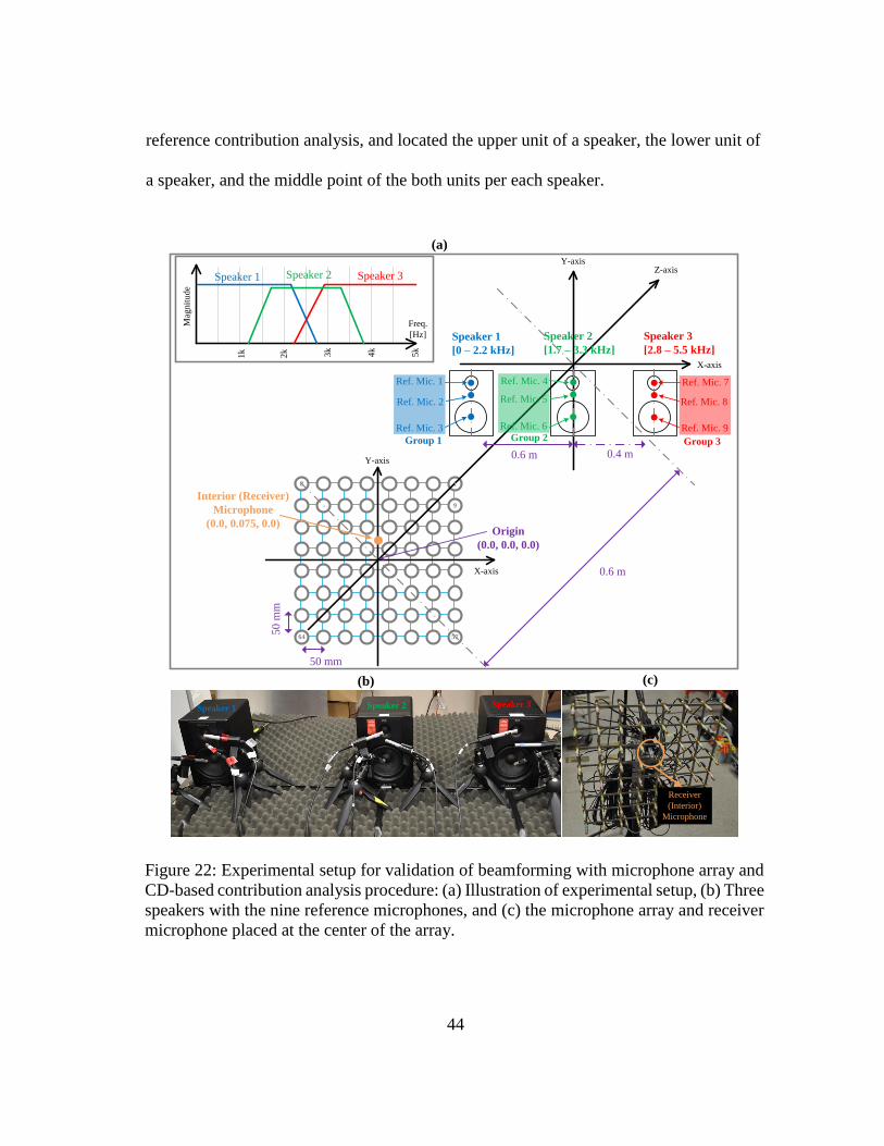
7.3 Experimental Setup for Validation

For the validation of beamforming based contribution, experimental data was

acquired with the configuration as shown in Figure 22. 3 speakers were located with

distances 0.6 m and 0.4 m, respectively. The speakers were driven by three independent,

filtered white noise signals using NI PXI-4461 for two speakers and B&K PULSE 3560-

B-130 for one speaker. The excited signals as shown in Figure 22(a) were low-pass

filtered white noise up to 2.2 kHz for speaker 1, band pass filtered white noise from 1.7

kHz to 3.3 kHz for speaker 2, and band pass filtered white noise from 2.8 to 5.5 kHz. 9

B&K Type 4189-A-021 (1/2”) microphones were used as reference microphones for the

44

reference contribution analysis, and located the upper unit of a speaker, the lower unit of

a speaker, and the middle point of the both units per each speaker.

Speaker 3Speaker 2Speaker 1

Receiver

(Interior)

Microphone

Speaker 1

[0 – 2.2 kHz]

Y-axis

X-axis

57

18

9

Y-axis

X-axis

Z-axis

Origin

(0.0, 0.0, 0.0)

50

mm

50 mm

Interior (Receiver)

Microphone

(0.0, 0.075, 0.0)

0.4 m0.6 m

Speaker 2

[1.7 – 3.3 kHz]

Speaker 3

[2.8 – 5.5 kHz]

0.6 m

Ref. Mic. 1

Freq.

[Hz]

Mag

nit

ude

2k 3k

4k

5k

Speaker 3Speaker 2Speaker 1

1k

Ref. Mic. 2

Ref. Mic. 3

Ref. Mic. 7

Ref. Mic. 8

Ref. Mic. 9

Ref. Mic. 4

Ref. Mic. 5

Ref. Mic. 6

64

(a)

(b) (c)

Group 1 Group 2 Group 3

Figure 22: Experimental setup for validation of beamforming with microphone array and

CD-based contribution analysis procedure: (a) Illustration of experimental setup, (b) Three

speakers with the nine reference microphones, and (c) the microphone array and receiver

microphone placed at the center of the array.

45

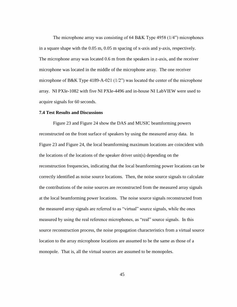
The microphone array was consisting of 64 B&K Type 4958 (1/4”) microphones

in a square shape with the 0.05 m, 0.05 m spacing of x-axis and y-axis, respectively.

The microphone array was located 0.6 m from the speakers in z-axis, and the receiver

microphone was located in the middle of the microphone array. The one receiver

microphone of B&K Type 4189-A-021 (1/2”) was located the center of the microphone

array. NI PXIe-1082 with five NI PXIe-4496 and in-house NI LabVIEW were used to

acquire signals for 60 seconds.

7.4 Test Results and Discussions

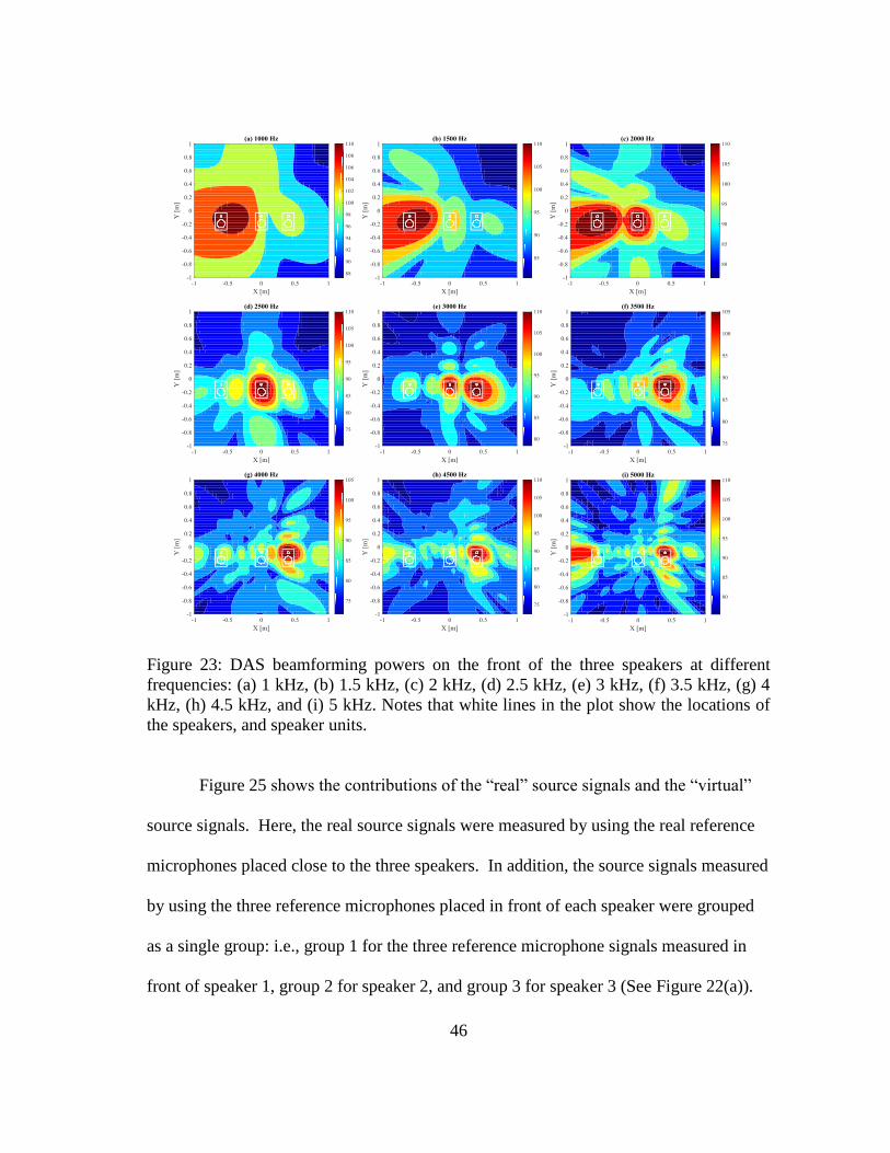
Figure 23 and Figure 24 show the DAS and MUSIC beamforming powers

reconstructed on the front surface of speakers by using the measured array data. In

Figure 23 and Figure 24, the local beamforming maximum locations are coincident with

the locations of the locations of the speaker driver unit(s) depending on the

reconstruction frequencies, indicating that the local beamforming power locations can be

correctly identified as noise source locations. Then, the noise source signals to calculate

the contributions of the noise sources are reconstructed from the measured array signals

at the local beamforming power locations. The noise source signals reconstructed from

the measured array signals are referred to as “virtual” source signals, while the ones

measured by using the real reference microphones, as “real” source signals. In this

source reconstruction process, the noise propagation characteristics from a virtual source

location to the array microphone locations are assumed to be the same as those of a

monopole. That is, all the virtual sources are assumed to be monopoles.

46

Figure 23: DAS beamforming powers on the front of the three speakers at different

frequencies: (a) 1 kHz, (b) 1.5 kHz, (c) 2 kHz, (d) 2.5 kHz, (e) 3 kHz, (f) 3.5 kHz, (g) 4

kHz, (h) 4.5 kHz, and (i) 5 kHz. Notes that white lines in the plot show the locations of

the speakers, and speaker units.

Figure 25 shows the contributions of the “real” source signals and the “virtual”

source signals. Here, the real source signals were measured by using the real reference

microphones placed close to the three speakers. In addition, the source signals measured

by using the three reference microphones placed in front of each speaker were grouped

as a single group: i.e., group 1 for the three reference microphone signals measured in

front of speaker 1, group 2 for speaker 2, and group 3 for speaker 3 (See Figure 22(a)).

47

The three virtual source signals were reconstructed from the array microphone signals at

the maximum beamforming locations of 1.5 kHz (Figure 23(b) and Figure 24(b)), 2.5

kHz (Figure 23(d) and Figure 24(d)), and 3.5 kHz (Figure 23(f) and Figure 24(f)). The

maximum contribution (i.e., the total of all the three contributions) in percent indicate

how much real or virtual source signals are correlated with the interior microphone

signal measured at the center of the array. The total contributions of the virtual source

signals are mostly higher than those of the real source signals, indicating that the effects

of background noise on the contributions of the real source signals are higher than those

of the virtual source signals since the virtual source locations can be closer to the

speakers than the real microphone locations. Due to the same reason, the contributions

of the virtual source signals in low, mid, and high frequency regions can be separated

better than those of the real signal groups. For example, speaker 1 generated low

frequency noise (e.g., below 1.7 kHz) dominantly. Thus, the contributions of real signal

group 1 and virtual source 1 are dominant in this frequency region. When comparing

Figure 25(a) and Figure 25(b) in the low frequency region, the contributions of virtual

source 1 is higher than those of real signal group 1 since the real reference microphones

close to speaker 1 can measure more noise generated from the two other speakers than

the virtual microphone at the virtual source 1 location. It is again because the distance

between the three reference microphones and speaker 1 is larger than the distance

between the virtual source location and speaker 1.

As shown in this section, the proposed procedure using the array microphones for

the prediction of the virtual source signals is innovative in that (1) it does not require

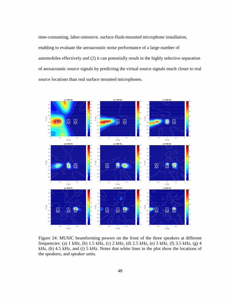
48

time-consuming, labor-intensive, surface-flush-mounted microphone installation,

enabling to evaluate the aeroacoustic noise performance of a large number of

automobiles effectively and (2) it can potentially result in the highly selective separation

of aeroacoustic source signals by predicting the virtual source signals much closer to real

source locations than real surface mounted microphones.

Figure 24: MUSIC beamforming powers on the front of the three speakers at different

frequencies: (a) 1 kHz, (b) 1.5 kHz, (c) 2 kHz, (d) 2.5 kHz, (e) 3 kHz, (f) 3.5 kHz, (g) 4

kHz, (h) 4.5 kHz, and (i) 5 kHz. Notes that white lines in the plot show the locations of

the speakers, and speaker units.

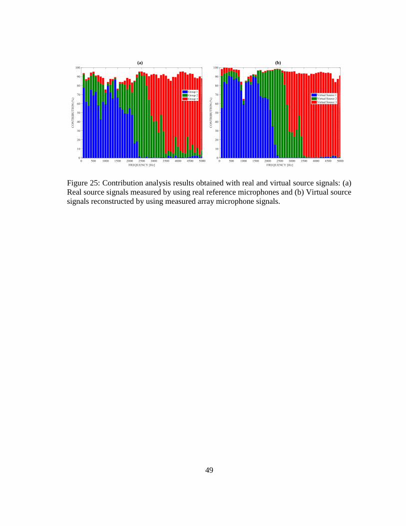
49

(a) (b)

Figure 25: Contribution analysis results obtained with real and virtual source signals: (a)

Real source signals measured by using real reference microphones and (b) Virtual source

signals reconstructed by using measured array microphone signals.

50

8. CONCLUSIONS

In this thesis, the contribution analysis method based on the Cholesky

Decomposition (CD) is proposed to decompose the measured interior noise spectra in an

automobile into physically meaningful, uncorrelated contributions of the external

aeroacoustic noise sources. An experiment with two speakers driven by two

independent white noise sources was conducted for the validation of the proposed

method. Through the two speaker experiment, it is shown that the contribution of both

speakers is successfully decomposed: each contribution can be associated with the noise

radiated from one of the speakers.

The automobile test at the two traveling speeds, 65 mph and 80 mph, was

conducted with 64 exterior microphones and 4 interior microphones. From the

contribution analysis results of the experimental data, the first nine highest contributions

to the interior noise were observed at the microphone groups of the upper area of the

front left window, the upper area of the front right window, the lower area of the front

left window, the hood, the lower area of the front right window, the lower area of the

rear right window, and the upper area of the rear right window. The aeroacoustic noise

with high contributions at the windows may be dominantly generated from the side

mirrors and the A-pillars. Through the comparisons of the automobile contribution

analysis results, it was shown that the contribution of the windows increased when the

vehicle speed increased. Regarding the effects of the seat position on the contribution,

the higher contribution could be obtained from the window closer to the specific seat of

interest.

51

The microphone-array-measurement-based contribution analysis procedure was

validated by conducting the experiment with three speakers driven by the independent

source signals. In the near future, this procedure will be used to evaluate a large number

of aeroacoustic automobile designs since it does not require the time-consuming and

labor-intensive installation of the surface-flush microphones.

52

REFERENCES

[1] S. K. Jha, "Characteristics and sources of noise and vibration and their control in

motor cars," Journal of Sound and Vibration, vol. 47, no. 4, pp. 543-558, 1976.

[2] D. Tcherniak and A. P. Schuhmacher, "Application of decomposition-based

technique in NVH source contribution analysis," in Proceedings of the

International Conference on Noise and Vibration Engineering (ISMA)-2008,

Leuven, Belgium, 2008.

[3] J. S. Bendat, "System identification from multiple input/output data," Journal of

Sound and Vibration,, vol. 49, no. 3, pp. 293-308, 1976.

[4] J. S. Bendat and A. G. Piersol, "Random data: Analysis and measurement

procedures," in Third Edition, Hoboken, NJ, John Wiley & Sons, 2000, pp. 240-

271.

[5] J. Y. Chung, M. J. Crocker and J. F. Hamilton, "Measurement of frequency

responses and the multiple coherence function of the noise-generation system of a

diesel engine," Journal of the Acoustical Society of America, vol. 58, pp. 635-642,

1975.

[6] A. G. Gonzalez, J. Rodrıguez, X. Sagartzazu, A. Schuhmacher and I. Isasa,

"Multiple coherence method in time domain for the analysis of the transmission

paths of noise and vibrations with non-stationary signals," in Proceedings of the

53

International Conference on Noise and Vibration Engineering (ISMA) 2010,

Leuven, Belgium, 2010.

[7] D. d. Klerk and A. Ossipov, "Operational transfer path analysis: Theory, guidelines

and tire noise application," Mechanical Systems and Signal Processing, vol. 24, no.

7, pp. 1950-1962, 2010.

[8] K. Wyckaert and H. V. d. Auweraer, "Operational analysis, transfer path analysis,

modal analysis: Tools to understand road noise problems in cars," No. 951251,

SAE Technical Paper, 1995.

[9] J. Plunt, "Finding and fixing vehicle NVH problems with transfer path analysis,"

Sound and Vibration, vol. 39, no. 11, pp. 12-17, 2005.

[10] P. Gajdatsy, K. Janssens, L. Gielen, P. Mas and H. V. D. Auweraer, "Critical

assessment of operational path analysis: Effect of coupling between path inputs,"

Journal of the Acoustical Society of America, vol. 123, no. 5, pp. 3876-3876, 2008.

[11] J. Putner, M. Lohrmann and A. Kaltenhauser, "Operational transfer path analysis

predicting contributions to the vehicle interior noise for different excitations from

the same sound source," in Proceedings of Inter-Noise 2012, New York City, NY,

United States, 2012.

[12] N. B. Roozen, Q. Leclere and C. Sandier, "Operational transfer path analysis

applied to a small gearbox test set-up," in Proceedings of Acoustics 2012, Nantes,

France, 2012.

54

[13] J. Putner, M. Lohrmann and H. Fastl, "Contribution analysis of vehicle exterior

noise with operational transfer path analysis," in Proceedings of Meetings on

Acoustics (ICA) 2013 Montreal, Montreal, Canada, 2013.

[14] W. Liu and D. J. Ewins, "Transmissibility properties of MDOF systems," in

Proceedings – SPIE the International Society for Optical Engineering, San Hose,

CA, United States, 1998.

[15] P. S. Varoto and K. G. McConnell, "Single point vs. multi point acceleration

transmissibility concepts in vibration testing," in Proceedings of the 16th

International Modal Analysis Conference (IMAC XVI), Santa Barbara, CA, United

States, 1998.

[16] A. M. R. Ribeiro, "On the generalization of the transmissibility concept," in

Proceedings of NATO/ASI Conference on Modal Analysis and Testing, Sesimbra,

Portugal, 1998.

[17] N. M. M. Maia, J. M. M. e. Silva and A. M. R. Ribeiro, "The transmissibility

concept in multi-degree-of-freedom systems," Mechanical Systems and Signal

Processing, vol. 15, no. 1, pp. 129-137, 2001.

[18] M. Fontul, A. M. R. Ribeiro, J. M. M. e. Silva and N. M. M. Maia,

"Transmissibility in structural coupling," in Proceedings of the International

Conference on Noise and Vibration Engineering (ISMA), Leuven, Belgium, 2004.

[19] N. M. M. Maia, M. Fontul and A. M. R. Ribeiro, "Transmissibility of forces in

multiple-degree-of-freedom systems," in Proceedings of the International

55

Conference on Noise and Vibration Engineering (ISMA 2006), Leuven, Belgium,

2006.

[20] D. Tcherniak, "Application of transmissibility matrix method to structure borne

path contribution analysis," in Proceedings of German Annual Conference on

Acoustics (NAG/DAGA 2009), Rotterdam, Holland, 2009.

[21] D. Tcherniak and Y. S. Ryu, "Developments in transmissibility matrix method in

application for structure borne noise path analysis," in Proceedings of Society of

Automotive Engineering of Japan (JSAE) 2009, Yokohama, Japan, 2009.

[22] H.-S. Kwon, Y.-J. Kim and J. S. Bolton, "Compensation for source nonstationarity

in multi-reference, scan-based nearfield acoustical holography," Journal of the

Acoustical Society of America, vol. 113, pp. 350-368, 2003.

[23] Y.-J. Kim, J. S. Bolton and H.-S. Kwon, "Partial sound field decomposition in

multireference near-field acoustical holography by using optimally located virtual

references," Journal of the Acoustical Society of America, vol. 115, no. 4, pp.

1641-1652, 2004.

[24] M. Cho, C. Oh, H. G. Kim and K. D. Ih, "On the ability of numerical solvers to

predict interior noise transmission of aerodynamic and aeroacoustic sources in a

simplified vehicle model," in Proceeding of Inter-Noise 2015, San Francisco, CA,

United States, 2015.

[25] L. E. Hunt, R. S. Dowans III, M. S. Kuester, E. B. White and W. S. Saric, "Flow

quality measurements in the Klebanoff-Saric Wind Tunnel," in Proceedings of

56

27th AIAA Aerodynamic Measurement Technology and Ground Testing

Conference, Anaheim, CA, United States, 2010.

[26] "Klebanoff-Saric Wind Tunnel Facility," 2013. [Online]. Available:

http://kswt.tamu.edu/facility/. [Accessed 26 09 2016].

[27] P. K. Kundu, I. M. Cohen and D. R. Dowling, "Fluid Mechanics," in 5th Ed.,

Waltham, MA, United States, Academic Press, 2012, p. 391.

57

APPENDIX

A. Contribution Analysis Software

The Contribution Analysis Software (CAS) was developed by using the

Graphical User Interface Development Environment (GUIDE) in MATLAB. Figure A1

shows the main window of the CAS. This software is designed to process new

measurement data as well as to reprocess previously processed data. The main

functionalities of the CAS are as follows:

• The CAS manages a file referred to as the CAS project file that includes raw time

data, experimental parameters, data processing parameters, post-processing parameters

for plots or export, and analyzed contribution results.

• The raw time data in the ASCII file format can be imported to the CAS as input

data.

• A user can select various data processing parameters including A-weighting, 1/1

or 1/3 octave/linear bands, time window functions, etc.

• The analysis results include individual source contributions, group contributions,

and overall contributions.

• The colors and names of reference channels or groups can be selected by a user.

• The groups of reference channels can be selected by a user.

• The analyzed contribution results can be plotted in the software and the plots can

be saved as image files.

• The analyzed results can also be exported to ASCII files.

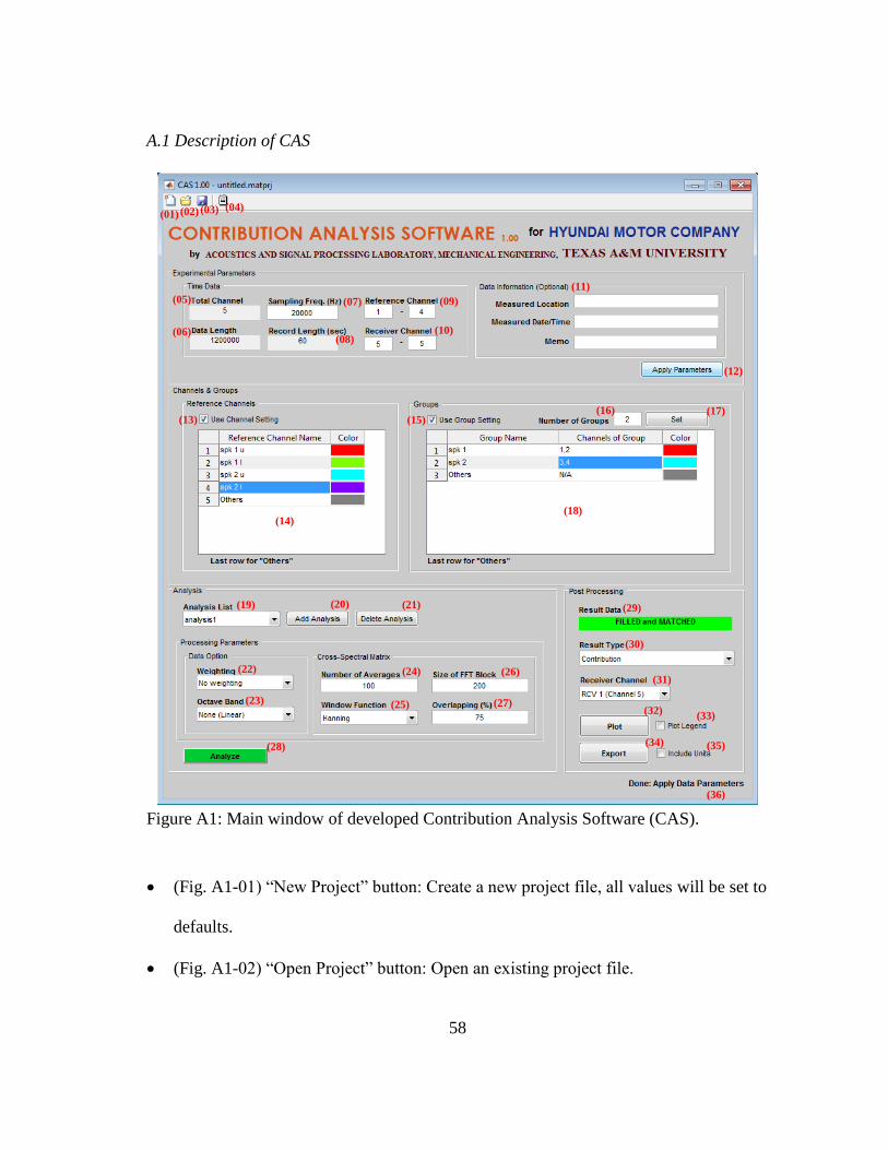
58

A.1 Description of CAS

(01) (02) (03) (04)

(05)

(06)(08)

(09)

(10)

(12)

(13)

(14)

(15)(16) (17)

(18)

(19) (20) (21)

(22)

(23)

(07)

(11)

(24)

(25)

(26)

(27)

(28)

(29)

(30)

(31)

(32)(33)

(34) (35)

(36)

Figure A1: Main window of developed Contribution Analysis Software (CAS).

(Fig. A1-01) “New Project” button: Create a new project file, all values will be set to

defaults.

(Fig. A1-02) “Open Project” button: Open an existing project file.

59

(Fig. A1-03) “Save Project” button: Save current data to the project file. When it is

pressed for the first time in a project, it save the project and a user needs to select a

path and filename. Once the project is saved, the click of this button will overwrite

the opened project file.

(Fig. A1-04) “Import Time Data” button: Open a popup window to import raw time

data in the ASCII file format.

(Fig. A1-05) “Total Channel” indicator: Show the total number of channels in the

loaded time data.

(Fig. A1-06) “Data Length” indicator: Show the time data length of the loaded time

data.

(Fig. A1-07) “Sampling Freq. (Hz)” input: Input the sampling frequency in Hertz

used in the loaded time data. A user has to input the sampling frequency: there is no

default value for this input.

(Fig. A1-08) “Record Length (sec)” indicator: Show the record length in second of

the loaded time data.

(Fig. A1-09) “Reference Channel” inputs: Input start and end channels of the

reference sensors. A user has to input these channel numbers.

(Fig. A1-10) “Receiver Channel” inputs: Input start and end channels of the receiver

sensors. A user has to input these channel numbers.

(Fig. A1-11) “Data Information (optional)” input: Input any descriptive information

on the current project.

60

(Fig. A1-12) “Apply Parameters” button: Apply the experimental parameters to the

current project. Prior to pressing this button, the raw time data has to be imported

and the sampling frequency, the reference channels, and the receiver channels have

to be filled out. The length of Table of Reference Channels will be changed by the

setting of Reference Channel.

(Fig. A1-13) “Use Channel Setting” checkbox:

Status Action

Checked Use the reference channel names and colors in the table for result plots.

Unchecked Use the default data.

(Fig. A1-14) Table of Reference Channels:

The last row of the table is for “Others”.

Column Description

First Column Reference channel number

Reference Channel Name Name for each reference channel.

Color Color for each reference channel. A user can choose a desired

color in the color pickup window.

(Fig. A1-15) “Use Group Setting” checkbox:

Status Action

Checked Use the group names and colors in the table below for result plots.

Unchecked Use the default data.

(Fig. A1-16) “Number of Groups” input: Number of groups to use.

(Fig. A1-17) “Set” button for number of groups: Set the length of Table of Groups

with Number of Groups.

(Fig. A1-18) Table of Groups:

The last row of the table is for “Others”.

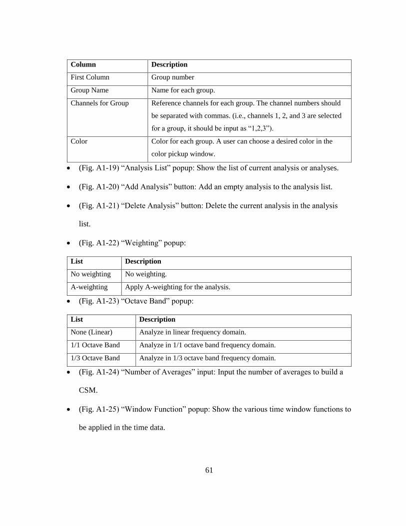
61

Column Description

First Column Group number

Group Name Name for each group.

Channels for Group Reference channels for each group. The channel numbers should

be separated with commas. (i.e., channels 1, 2, and 3 are selected

for a group, it should be input as “1,2,3”).

Color Color for each group. A user can choose a desired color in the

color pickup window.

(Fig. A1-19) “Analysis List” popup: Show the list of current analysis or analyses.

(Fig. A1-20) “Add Analysis” button: Add an empty analysis to the analysis list.

(Fig. A1-21) “Delete Analysis” button: Delete the current analysis in the analysis

list.

(Fig. A1-22) “Weighting” popup:

List Description

No weighting No weighting.

A-weighting Apply A-weighting for the analysis.

(Fig. A1-23) “Octave Band” popup:

List Description

None (Linear) Analyze in linear frequency domain.

1/1 Octave Band Analyze in 1/1 octave band frequency domain.

1/3 Octave Band Analyze in 1/3 octave band frequency domain.

(Fig. A1-24) “Number of Averages” input: Input the number of averages to build a

CSM.

(Fig. A1-25) “Window Function” popup: Show the various time window functions to

be applied in the time data.

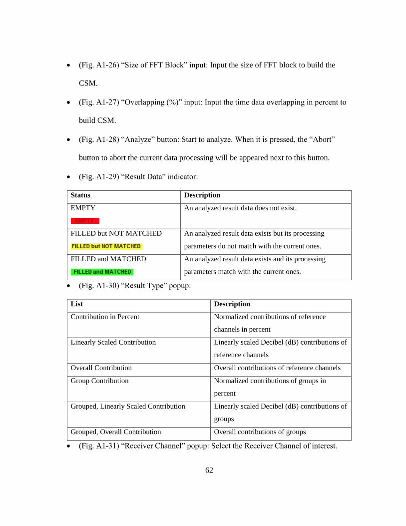
62

(Fig. A1-26) “Size of FFT Block” input: Input the size of FFT block to build the

CSM.

(Fig. A1-27) “Overlapping (%)” input: Input the time data overlapping in percent to

build CSM.

(Fig. A1-28) “Analyze” button: Start to analyze. When it is pressed, the “Abort”

button to abort the current data processing will be appeared next to this button.

(Fig. A1-29) “Result Data” indicator:

Status Description

EMPTY

An analyzed result data does not exist.

FILLED but NOT MATCHED

An analyzed result data exists but its processing

parameters do not match with the current ones.

FILLED and MATCHED

An analyzed result data exists and its processing

parameters match with the current ones.

(Fig. A1-30) “Result Type” popup:

List Description

Contribution in Percent Normalized contributions of reference

channels in percent

Linearly Scaled Contribution Linearly scaled Decibel (dB) contributions of

reference channels

Overall Contribution Overall contributions of reference channels

Group Contribution Normalized contributions of groups in

percent

Grouped, Linearly Scaled Contribution Linearly scaled Decibel (dB) contributions of

groups

Grouped, Overall Contribution Overall contributions of groups

(Fig. A1-31) “Receiver Channel” popup: Select the Receiver Channel of interest.

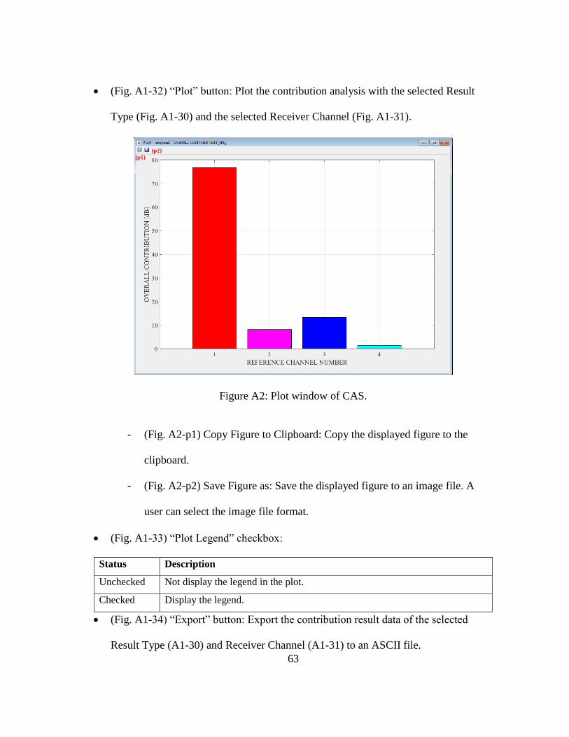
63

(Fig. A1-32) “Plot” button: Plot the contribution analysis with the selected Result

Type (Fig. A1-30) and the selected Receiver Channel (Fig. A1-31).

(p1)

(p2)

Figure A2: Plot window of CAS.

- (Fig. A2-p1) Copy Figure to Clipboard: Copy the displayed figure to the

clipboard.

- (Fig. A2-p2) Save Figure as: Save the displayed figure to an image file. A

user can select the image file format.

(Fig. A1-33) “Plot Legend” checkbox:

Status Description

Unchecked Not display the legend in the plot.

Checked Display the legend.

(Fig. A1-34) “Export” button: Export the contribution result data of the selected

Result Type (A1-30) and Receiver Channel (A1-31) to an ASCII file.

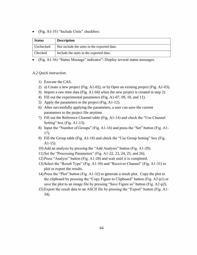
64

(Fig. A1-35) “Include Units” checkbox:

Status Description

Unchecked Not include the units in the exported data.

Checked Include the units in the exported data.

(Fig. A1-36) “Status Message” indicator”: Display several status messages.

A.2 Quick instruction.

1) Execute the CAS.

2) a) Create a new project (Fig. A1-02), or b) Open an existing project (Fig. A1-03).

3) Import a raw time data (Fig. A1-04) when the new project is created in step 2).

4) Fill out the experimental parameters (Fig. A1-07, 09, 10, and 11).

5) Apply the parameters to the project (Fig. A1-12).

6) After successfully applying the parameters, a user can save the current

parameters to the project file anytime.

7) Fill out the Reference Channel table (Fig. A1-14) and check the “Use Channel

Setting” box (Fig. A1-13).

8) Input the “Number of Groups” (Fig. A1-16) and press the “Set” button (Fig. A1-

17).

9) Fill the Group table (Fig. A1-18) and check the “Use Group Setting” box (Fig.

A1-15).

10) Add an analysis by pressing the “Add Analysis” button (Fig. A1-20).

11) Set the “Processing Parameters” (Fig. A1-22, 23, 24, 25, and 26).

12) Press “Analyze” button (Fig. A1-28) and wait until it is completed.

13) Select the “Result Type” (Fig. A1-30) and “Receiver Channel” (Fig. A1-31) to

plot or export the results.

14) Press the “Plot” button (Fig. A1-32) to generate a result plot. Copy the plot to

the clipboard by pressing the “Copy Figure to Clipboard” button (Fig. A2-p1) or

save the plot to an image file by pressing “Save Figure as” button (Fig. A2-p2).

15) Export the result data to an ASCII file by pressing the “Export” button (Fig. A1-

34).

M.S. Thesis - OAKTrust - Texas A&M University

Documents