MRP and Aggregate Planning

Material Requirements

Planning (MRP)

MRP

The logic for determining the number of

parts, components, and materials needed

to produce a product.

It also provides a schedule specifying

when each of these materials, parts, and

components should be ordered and

produced

Independent vs. Dependent

Demand

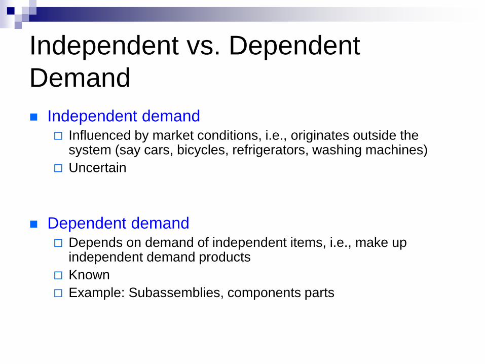
Independent demand Influenced by market conditions, i.e., originates outside the

system (say cars, bicycles, refrigerators, washing machines)

Uncertain

Dependent demand Depends on demand of independent items, i.e., make up

independent demand products

Known

Example: Subassemblies, components parts

Independent vs. Dependent

Demand

Demand Pattern for Independent

versus Dependent Items

Attribute Dependent

Demand

Independent

Demand

Nature of Demand No uncertainty Uncertainty

Goal Meet requirements

exactly

Meet demand for a

targeted service

level

Service Level 100% 100% difficult

Demand

occurrence

Often lumpy Often continuous

Estimation of

demand

By production

planning

By forecasting

How much to

order?

Known with

certainty

Estimate based on

past consumption

Key Differences: Dependent vs. Independent Demand

Material Requirements Planning (MRP)

MRP is a technique that has been employed since the

1940s and 1950s.

Joe Orlicky is known as the Father of MRP

The use and application of MRP grew through the

1970s and 1980s as the power of computer hardware

and software increased.

MRP gradually evolved into a broader system called

manufacturing resource planning (MRP II).

Material Requirements Planning

(MRP) MRP is a computerized inventory system

developed specifically to manage dependent demand items

MRP works backward from the due date using lead times to determine when and how much to order for

Subassemblies, component parts & raw materials

MRP MRP begins with a schedule for finished goods

that is converted into a schedule of requirements

for subassemblies, component parts and raw

materials needed to produce the finished items in

the specified time frame

MRP designed to answer the following questions

• What is needed ?

• How much is needed?

• When is it needed ?

MRP

MRP thus works with finished products, or end items,

and their constituent parts, called lower level items

According to one study, 80% of high performing

manufacturing plants have implemented MRP

MRP works well for assembling complex discrete

products produced in batches

Example: computers, consumer durables, furniture,

watches, trucks, generators, motors, machine tools

Inputs and Outputs of MRP

MRP MPS

BOM MRP Inventory Records

Planned Order Release

Work Order Purchase order Rescheduling

Notices

Master Production Schedule

A time table that specifies what (end item)

is to be made and when

Time period used for planning is called a

time bucket

MPS shows how many of each individual

item must be completed each period

Aggregate Production Plan and

MPS -- Amplifiers

How does MPS differ from AP-

Motors

Aggregate Production Plan - Cars

Hundai Motors: Month # of Cars

Jan 10,000 Feb 12,000

Mar 8,000

April 11,000

May 7,000

Weeks

of

January

I II III IV Total

Santro 1,200 2,000 2,500 700 6,400

Accent 700 950 1,300 250 3,200

Sonata 100 50 200 50 400

2,000 3,000 4,000 1,000 10,000

MASTER PRODUCTION SCHEDULE

1. Master Production Schedule

(MPS)

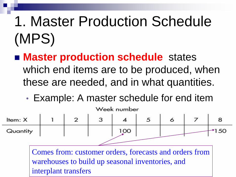
Master production schedule states

which end items are to be produced, when

these are needed, and in what quantities.

• Example: A master schedule for end item

X:

Comes from: customer orders, forecasts and orders from

warehouses to build up seasonal inventories, and

interplant transfers

2. Bill of Materials (BOM)

A document that lists the components, their description,

sequence in which the product is created and the

quantity of each required to make one unit of a product

Thus relationship between end items and lower level

items is described by the BOM

It depicts exactly how a firm makes the item in the

master schedule

Extremely important to have BOM correct to have

accurate material estimates

2. Bill of Materials (BOM)

The BOM file is often called the product

structure file or product tree because it

shows how a product is put together

Assembly Diagram & Product

Structure Tree

Product Structure Tree of

Sub-Assembly

Product Structure Tree of Product

X With Levels

Visual description of the requirements in a bill of materials, where all components are listed by levels

(Highest)

(Lowest)

Indented Parts List for Meter A and Meter B

A Product Structure Tree

Note: Restructuring the BOM so that multiple occurrences of a component all coincide

with the lowest level at which the component occurs

BOM & Product Structure Tree (An

Example)

Partial Bill

of Materials for a Bicycle

3. Inventory Record

Third input in MRP

It tells us about the status of inventory of an item

at present, or in a given interval of time in the

coming future

On hand

On Order (scheduled receipt)

Lead time

Lot size

Code

Outputs of MRP

(Primary Reports) Planned order receipt – A schedule indicating the

quantity that is planned to arrive at the beginning of a period

Planned Order release – Authorizes the execution of planned orders (work order + purchase order). To determine planned order release, count backward from the planned order receipt using the lead time

Order changes report – Changes to planned order, including revisions for due dates or order quantities and cancellation of orders

Outputs of MRP

(Secondary Reports)

Performance control report – evaluate

system performance, deviations from

plans, missed deliveries, and stock outs

Exception reports – attention to major

discrepancies such as late and overdue

orders, requirements for non-existence

parts, reporting errors

MRP Terminologies

Gross Requirements: Total demand for an item during each time period. For end items, these quantities are shown in the master production schedule For components, these quantities are derived from the planned

order releases of their immediate parents

Scheduled Receipts: Orders that have been released and scheduled to be received from vendors by the beginning of a period

Projected On-Hand: The expected amount of inventory that will be on hand at the beginning of each time period (SR + Avl inv from last period)

MRP Terminologies

Net requirements: The actual amount needed in each time period

Planned Order Receipts: The quantity expected to be received from a vendor or in-house shop at the beginning of the period in which it is shown. It is the amount of an order that is required to meet a net requirement in the period. Under lot-for-lot ordering, this quantity will equal net requirements.

Under lot-size ordering, this quantity may exceed net requirements. Any excess is added to available inventory in the next time period.

MRP Terminologies

Planned Order Release: Indicates a

planned amount to order in the beginning

of each time period; equals planned-order

receipts offset by lead time.

Format of MRP

Week Number 0 1 2 3 4 5 6 7 8

Item:

Gross requirements

Scheduled receipts

Projected on hand

Net requirements

Planned-order

receipts

Planned-order

releases

MRP Explosion

The MRP process of determining

requirements for lower level items

(subassemblies, components, raw

materials) based on the master production

schedule

Planned Order Report

PERIOD

ITEM 1 2 3 4 5

A X1 X2 X3

B Y1 Y2

C Z1 Z2 Z3

Lot Sizing in MRP Systems

Lot-for-Lot (L4L)

Sets planned orders to exactly match the net requirements. Eliminates holding costs

Economic order quantity (EOQ)

Balances setup and holding costs

Lot Sizing in MRP Systems

Least total cost (LTC)

Balances carrying cost and setup cost for various lot sizes, and selects the one where they are most nearly equal

Least unit cost (LUC)

Adds ordering and inventory carrying costs for each trial lot size and divides by number of units in each lot size, picking the lot size with the lowest unit cost

Lot-for-Lot

MRP and Capacity Planning

MRP , as it was originally introduced, considered

only materials. MRP does not compare the

planned orders to the available capacity. Most

MRP plans assume infinite loading; that is an

infinite amount of capacity is available, which is

not realistic. Individual machines or work

centres may have capacity shortages and

backlogs of work to be completed

We therefore need capacity planning.

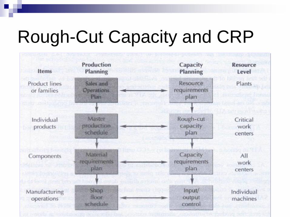
Two Approaches to Capacity

Planning Rough-cut capacity planning

Uses the MPS (end item) as the source of product

demand information

Capacity determination at critical work centres

Capacity Requirement Planning

Completed at the component level rather than at the

end item level

Uses planned order release from MRP

Capacity determination at all work centres

Focused on critical

work centres

Rough-Cut Capacity and CRP

Capacity Requirements

Planning (CRP)

CRP determines if all the work centres

involved have the capacity to implement

the MRP plan.

A load profile compares weekly loads

needs against a profile of actual capacity.

CAPACITY REQUIREMENT PLANNING

Workload for a Work Center

Capacity

Work center Effective Capacity/week (2 machines):

(# machines)×(# shifts)× (# of hours/shift)× (# days/week)×

(utilization)×(efficiency)

Utilization: Time working / Time available

Efficiency: Actual output / standard output

Load: Standard hours of work assigned to a production facility

Load % = (Load / Capacity)×100%

Scheduled Workload for a Work

Center

161.5

137.8

190.3

128.8

2m/c * 2 shifts/day * 10 hours/shift * 5 days/week * 85%(m/c Util) * 0.95 (m/c efficiency) =161.5 hrs/week

Capacity Levelling

Work Overtime

Selecting an alternative work center

Subcontract

Scheduling part of work of week 11 into

week 10

Renegotiate due date

Safety Stock

It would seem that an MRP inventory system should not require

safety stock. Practically, however, there may be exceptions.

Typically SS built-into projected on-hand inventory

Why is safety stock necessary?

Two types of uncertainties are prevalent

A. The quantity of components received (soln: SS)

I. Poor quality may result in quantity loss

II. Reliability in supplier may result in quantity uncertainty

B. Timing of the receipts (solution: safety time)

A. Machine breakdowns, fluctuations in staffing

Updating MRP Schedules

Updating MRP schedule is required because

Customers may cancel or amend order

Suppliers could default on supply

Unexpected disruptions in manufacturing

Two techniques of updating

Regeneration, i.e., re plan the whole system (run MRP from scratch, updated periodically, 100% replacement of the existing information)

Net change

Instead of running the entire MRP system, schedules of components pertaining to portions where changes have happened are updated.

Applies to sub-set of data as opposed to regeneration

MRP Dynamics - System

Nervousness MRP systems work best under conditions of reasonable

stability

Frequent changes in an MRP system leads to major

changes in the order profiles for lower level

subassemblies or components creating havoc for

purchasing and production departments. This is called

system nervousness Tool helpful in reducing system

nervousness

Time fences

Freezing the Master Schedule

Time Fences in MPS

Period

“frozen”

(firm or

fixed)

“slushy”

somewhat

firm

“liquid”

(open)

1 2 3 4 5 6 7 8 9

Time Fences divide a scheduling time horizon into three

sections or phases, referred as frozen, slushy, and liquid.

Strict adherence to time fence policies and rules.

Pegging

Tracing upward in the BOM from the

component to the parent item. By pegging

upward, the production planner can

determine the cause for the requirement

and make a judgement about the

necessary for a change in schedule

Reduction in inventory

Increased customer satisfaction due to

meeting delivery schedules

Faster response to market changes

Improved labor & equipment utilization

Better inventory planning & scheduling

MRP Benefits

Benefits of MRP

Ability to easily determine inventory

usage by backflushing

Back flushing: Exploding an end item’s

bill of materials to determine the

quantities of the components that were

used to make the item.

MRP – Problems Encountered

Data integrity is low

Not frequent updates of databases when

changes takes place

Uncertainties related to lead time and

quantity delivered

Requirements of Successful

MRP System

Computer and necessary software

Accurate and up-to-date

Master schedules

Bills of materials

Inventory records

User knowledge

Management support

Evolved from MRP in 1980s

Didn’t replace or improve MRP. Rather expanded the scope

to include capacity requirements planning and to involve

other functional areas of the organization:

Purchasing, Manufacturing, Marketing, Finance,

Logistics

MRP II employed common database and an integrated

platform where sales, inventory, purchasing transactions

were updated in both inventory and accounting applications

Manufacturing Resource Planning

(MRP II)

Market

Demand

Production

plan

Problems?

Rough-cut

capacity planning

Yes No Yes No

Finance

Marketing

Manufacturing

Adjust

production plan

Master

production schedule

MRP

Capacity

planning

Problems? Requirements

schedules

Ad

just

maste

r sch

ed

ule

An Overview of MRP II

Aggregate Sales and

Operations Planning

Planning Level and Activities

Planning Stages in Operation

Aggregate planning is a big picture approach to production plan to meet the demand throughout the year or so.

It is not concerned with individual products, but with a single aggregate product representing all products.

For example, in a TV manufacturing plant, the aggregate planning does not go into all models and sizes. It only deals with a single representative aggregate TV.

All models are lumped together and represent a single

product; hence the term aggregate planning.

Aggregate Planning

What does Aggregate Mean?

Overall terms Product families or product lines rather than individual

products, thus the term aggregate

In other words, one “collapses” a multi-product firm to

a single-product firm, the “product” being aggregate

units of production

Big picture approach to planning

Aggregate, for example # bicycles to be produced,

but would not identify bicycles by colour, size, type

etc.

How does MPS differ from AP

Aggregation (Example)

Suppose a bicycle manufacturer makes three models (Standard,

Deluxe, Sports)

Time: Standard: 30 m/c hours, Deluxe: 60 m/c hours, Sports: 90 m/c

hours

Thus manufacturing 1 deluxe model is equivalent to manufacturing 2

standard models. 1 sports model is equivalent to manufacturing 3

standard models from resource consumption perspective

Thus a monthly demand of 1000 standard cycles, 500 deluxe, and

250 sports can be aggregated as 2750 standard models on the

basis of machine hours

Identifying Aggregate Units of

Production Product

Family

Material cost/

Unit (Rs)

Revenue /

unit (Rs)

Prodn. Time

/unit

(includes

setup time)

% share of

units sold

A 15 54 5.76 10

B 7 30 3.04 25

C 9 39 3.88 20

D 12 49 5.00 10

E 9 36 3.66 20

F 13 48 4.37 15

Material cost / aggregate unit = 15*0.10+7*0.25+9*0.20+12*0.10+9*0.20+13*0.15 = Rs 10

Revenue / aggregate unit = 54*0.10+30*0.25+39*0.20+49*0.10+36*0.20+48*0.15 = Rs 40

Production time / agg. unit = 5.76*0.1+3.04*.25+3.88*0.20+5*0.1+3.66*0.20+4.37*0.15 = 4 hrs

Why Aggregate Planning?

A plan for orderly and systematic change

of production capacity to meet peaks and

valleys of expected customer demand

Getting the most output for the amount of

resources available, which is important in

times of scarce production resources

Why Aggregate Planning?

Provides for fully loaded facilities, thus

minimizing

Overloading and under loading

Minimizing cost over the planning period

Adequate production capacity to meet

expected aggregate demand

Optimize balance between demand and

supply

Steps in Aggregate Planning

1. Begin with sales forecast for each product that

indicates the quantities to be sold in each time

period (usually months, or quarters) over the

planning horizon (3-18 months)

2. Total all the individual product or service

forecast into one aggregate demand.

Steps in Aggregate Planning

3. Determine capacities (regular time, OT,

subcontracting) for each period

4. Determine unit costs for regular time, OT,

subcontracting, holding inventories, back

orders, layoffs etc.

5. Identify company policy (chase, level, mixed)

Steps in Aggregate Planning

6. Develop alternative plans and compute

cost for each

7. Select the best alternative that satisfies

company’s objectives

Strategies for Meeting Demand

Proactive

Alter demand to match capacity

Reactive

Alter capacity to match demand

Mixed

Some of each

Strategies for Meeting Demand

Proactive strategies

Influencing Demand

Offer discounts and promotions

Increase advertising in slack periods

Counter seasonal products

Lawnmowers (summer) and snow-blowers (winter)

Strategies for Meeting Demand

Reactive Strategies

Changing inventory levels

Vary workforce size (hiring and lay-off)

Varying shifts

Varying working hours

Varying production through overtime or idle time

Subcontracting

Inputs and Costs in AP

Decision Variable Costs

Varying work force size Hiring, training, firing costs

Using Overtime Overtime costs

Varying inventory levels Holding costs

Accepting back orders Back order costs

Subcontracting others Subcontracting costs

Outputs of Aggregate Planning

Total cost of a plan

Projected levels of

Inventory held

Output from

Regular time, overtime, subcontracting

Employment

Graphical Method

Popular technique

Easy to understand and use

Trial-and-error approaches that do not guarantee an optimal solution

Require only limited computations

Graphical Method Month Expected

Demand

Production

Days

Demand /

day

Avg. daily

demand

Jan 900 22 41 50

Feb 700 18 39 50

March 800 21 38 50

April 1200 21 57 50

May 1500 22 68 50

June 1100 20 55 50

6,200 124

Graphical Method

Note: Forecast differs from average demand

Aggregate Planning Techniques

Two pure forms of aggregate planning strategies

Level Production

Maintain constant workforce and adjust inventory

Chase Demand

Hiring and Firing people

Aggregate Planning Techniques

Mixed Strategy

Combination of

Overtime, under time, & subcontracting

Part Time employees

Hiring and firing

Inventory

Backordering

Note: When one alternative: Pure Strategy

When two or more are selected: Mixed strategies

Level Production Strategy

It is an aggregate planning in which monthly production

is uniform

Requires no overtime, no change in work force levels,

and no subcontracting

Toyota and Nissan follow this strategy

Finished goods inventory go up or down to buffer the

difference between demand and production

Level Production Strategy

LEVEL PRODUCTION STRATEGY

Assume begin inventory: 2000

Chase Production Strategy

It attempts to achieve output rates that match demand

forecast for that period.

This strategy can be accomplished by:

Vary workforce levels (hiring and firing)

Service businesses use because they don’t have the

option to build inventory of their product

Chase Production Strategy

CHASE DEMAND STRATEGY

Chase vs. Level

Chase Approach

Advantages

Investment in inventory

is low

Labor utilization in high

Disadvantages

The cost of adjusting

output rates and/or

workforce levels

Level Approach

Advantages

Stable output rates and

workforce

Disadvantages

Greater inventory costs

Increased overtime and

idle time

Resource utilizations vary

over time

Mixed Strategy

For most firms, neither a chase strategy

nor a level strategy is likely to prove ideal,

so a combination of options must be

achieved to meet demand and minimize

cost

More complex than pure ones but typically

yield a better strategy

OVERTIME & SUBCONTRACTING

Linear Programming

Approaches to AP

Finds minimum cost solution related to

regular labour time, overtime,

subcontracting, caring inventory, and costs

associated with changing the size of

workforce

Mathematical Techniques to

Aggregate Planning

Linear Programming

Optimal solutions

Cost minimization

Profit maximization

Appropriate when cost and variable

relationships are linear

Application in industry limited

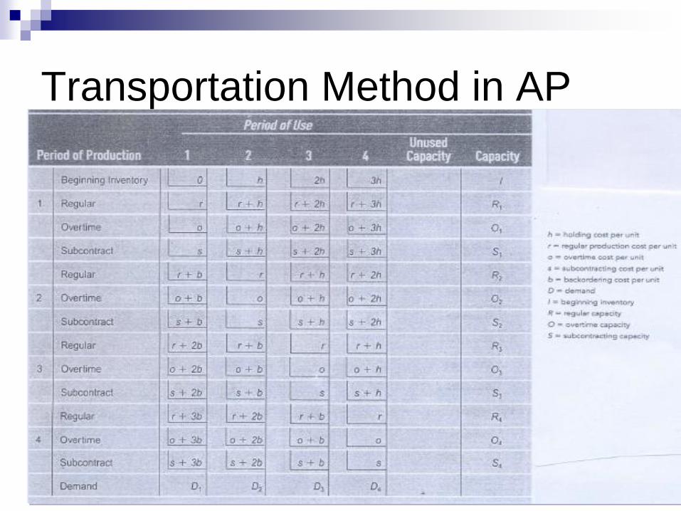
Transportation Method in AP

Transportation Method in AP

Transportation Method

(An Example)

Total Costs

Period Demand Regular

Production

Overtime Subcontract End

Inventory

1 900 1000 100 0 500

2 1500 1200 150 250 600

3 1600 1300 200 500 1000

4 3000 1300 200 500 0

Total 7000 4800 650 1250 2100

Total Cost: 4800×$20+650×$25+1250×$28+2100×$3 = $153,550

Transportation Method

(Second Example – Prob 7)

Transportation Method: Cost of

Plan Period 1: 50($0)+300($50)+50($65)+50($80)=$22,250

Period 2: 400($50)+50($65)+100($80)=$31,250

Period 3: 50($81)+450($50)+50($65)+200($80)=$45,800

Total Cost: $99,300

Simulation Models in AP

Development of computerized model under variety of conditions to find reasonably acceptable solutions

Advantages Lends itself to problems that are difficult to solve

mathematically

Experimenting system behaviour without any risk

Compresses time to understand system

Understand system behaviour under wide range of conditions

Simulation Models in AP

Limitations

Simulation does not produce optimal

solutions, it merely indicates approximate

behaviour for a set of inputs

Simulations are based on models, and

models are only approximation of reality

Summary of Aggregate

Planning Techniques

Technique Solution

Approach

Characteristics

Spreadsheet Heuristic (trial and

error)

Intuitively appealing,

easy to understand,

solution not optimal

Linear Programming Optimizing Computerized

Simulation Heuristic (trial and

error)

Computerized

models can be

examined under

various scenarios