MPH Program, Biostatistics II February 15, 2011 W.D. Dupontbiostat.mc.vanderbilt.edu/wiki/pub/Main/BiostatIILectureNotes/02... · MPH Program, Biostatistics II W.D. Dupont February

MPH Program, Biostatistics II W.D. Dupont

February 15, 2011

2: Multiple Linear Regression 2.1

We usually assume that the patient’s response y is causally related tothe variables xi1, xi2, …, xik through the model. These latter variablesare called covariates or explanatory variables; y is called thedependent or response variable.

i are independently distributed and has a normal distribution with mean 0 and standard deviation , and

1. The Model

yi = + 1xi1 + 2xi2 + … + kxik + i

xi1, xi2, …, xik are known variables,

yi is the value of the response variable for the ith patient.

, 1, 2, …, k are unknown parameters,

where


February 15, 2011


2. Reasons for Multiple Linear Regression

a) Adjusting for confounding variables

To investigate the effect of a variable on an outcome measure adjusted for the effects of other confounding variables.

01

20

1

0

1

2

3

4

y =

x1

+ 2x 2

x1

x2

3-4

2-3

1-2

0-1

ii) If yi increases rapidly with and xi1, and xi1 and xi2 are highly correlated then the rate of increase of yi with increasing xi1 when

xi2 is held constant may be very different from this rate of increase when xi2 is not restrained.

i) 1 estimates the rate of change of yi with xi1 among patients with the same values of xi2, xi3, …, xik.

NOTE: The model assumes that the rate of change of yi with xi1 adjusted for xi1, xi2, …, xik is the same regardless of the values of these latter variables.


February 15, 2011


b) Prediction

To predict the value of y given x1, x2, …, xk

3. Estimating Parameters

Let be the estimate of yi given xi1, xi2, …, xik.

We estimate a, b1, …, bk by minimizing ( )y y 2

1 1 2 2ˆ ...i i i k iky a b x b x b x

may be rewritten

1 1 1 2 2 2ˆ ( ) ( ) ... ( ).i i i i k ik ky y b x x b x x b x x {2.1}

We estimate the expected value of yi among subjects whose covariate values are identical to those of the ith patient by . The equationîy

1 1 2 2ˆ ... .i i i k iky a b x b x b x

1 1 2 2ˆThus, when , ,..., and .i i i ik ky y x x x x x x

4. Expected Response in the Multiple Model

The expected value of both yi and given her covariates is

1 1 2 2ˆ[ ] E[ ] ... . i i i i i i k iky y x x x x x

îy

Follow-up information on coronary heart disease is also provided.

This data set is a subset of the 40 year data from the FraminghamHeart Study that was conducted by the National Heart Lung and BloodInstitute. Recruitment of patients started in 1948. At that time of thebaseline exams there were no effective treatment for hypertension.

5. Framingham Example: SBP, Age, BMI, Sex and Serum Cholesterol

a) Preliminary univariate analysis

The Framingham data set contains data on 4,699 patients. On each patient we have the baseline values of the following variables:

sbp Systolic blood pressure in mm Hg.

age Age in years

scl Serum cholesterol in mg/100ml

bmi Body mass index in kg/m2

sex 1 = Men

2 = Women


February 15, 2011


Source | SS df MS Number of obs = 4690---------+------------------------------ F( 1, 4688) = 565.07

Model | 262347.407 1 262347.407 Prob > F = 0.0000Residual | 2176529.37 4688 464.276742 R-squared = 0.1076---------+------------------------------ Adj R-squared = 0.1074

Total | 2438876.78 4689 520.127271 Root MSE = 21.547

------------------------------------------------------------------------------sbp | Coef. Std. Err. t P>|t| [95% Conf. Interval]

---------+--------------------------------------------------------------------bmi | 1.82675 .0768474 23.771 0.000 1.676093 1.977407

_cons | 85.93592 1.9947 43.082 0.000 82.02537 89.84647------------------------------------------------------------------------------

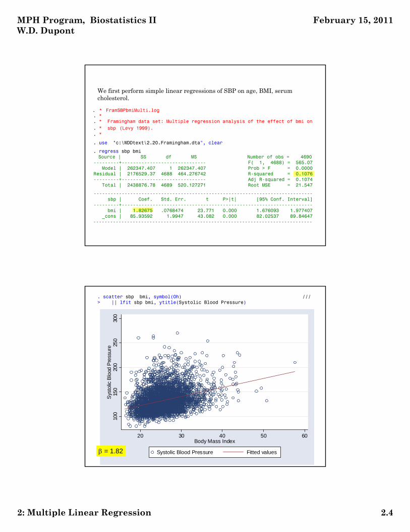
We first perform simple linear regressions of SBP on age, BMI, serum cholesterol.

. * FramSBPbmiMulti.log

. *

. * Framingham data set: Multiple regression analysis of the effect of bmi on

. * sbp (Levy 1999).

. *

. use "c:\WDDtext\2.20.Framingham.dta", clear

. regress sbp bmi

. scatter sbp bmi, symbol(Oh) ///> || lfit sbp bmi, ytitle(Systolic Blood Pressure)

100

150

200

250

300

Sys

tolic

Blo

od P

ress

ure

20 30 40 50 60Body Mass Index

Systolic Blood Pressure Fitted values = 1.82


February 15, 2011


. regress sbp age



Total | 2442444.90 4698 519.890358 Root MSE = 20.954


---------+--------------------------------------------------------------------age | 1.057829 .0359468 29.428 0.000 .9873561 1.128301

_cons | 84.06298 1.68302 49.948 0.000 80.76347 87.36249------------------------------------------------------------------------------

. scatter sbp age, symbol(Oh) ///> || lfit sbp age, ytitle(Systolic Blood Pressure)

100

150

200

250

300

Sys

tolic

Blo

od P

ress

ure

30 40 50 60 70Age in Years



February 15, 2011


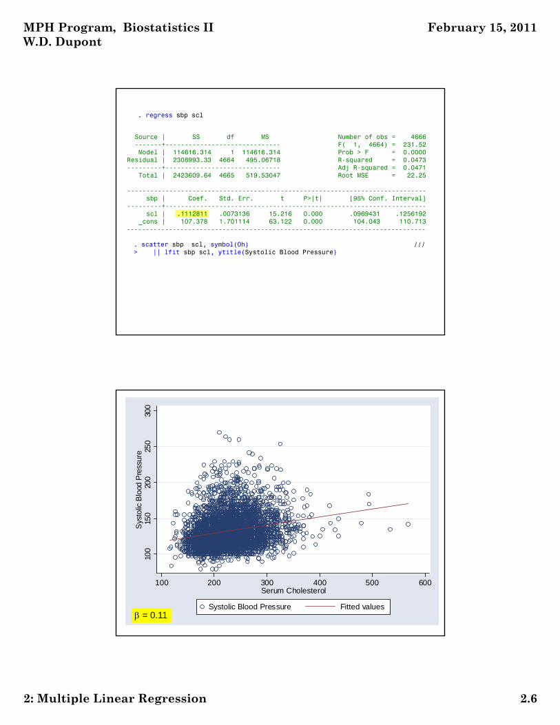
. regress sbp scl

Source | SS df MS Number of obs = 4666-------+------------------------------ F( 1, 4664) = 231.52Model | 114616.314 1 114616.314 Prob > F = 0.0000

Residual | 2308993.33 4664 495.06718 R-squared = 0.0473---------+------------------------------ Adj R-squared = 0.0471

Total | 2423609.64 4665 519.53047 Root MSE = 22.25


---------+--------------------------------------------------------------------scl | .1112811 .0073136 15.216 0.000 .0969431 .1256192

_cons | 107.378 1.701114 63.122 0.000 104.043 110.713------------------------------------------------------------------------------

. scatter sbp scl, symbol(Oh) ///> || lfit sbp scl, ytitle(Systolic Blood Pressure)

100

150

200

250

300

Sys

tolic

Blo

od P

ress

ure

100 200 300 400 500 600Serum Cholesterol



February 15, 2011


Note that the importance of a parameter depends not only on its magnitudebut also on the range of the corresponding covariate. For example, the sclcoefficient is only 0.11 as compared to 1.83 and 1.06 for bmi and age.However, the range of scl values is from 115 to 568 as compared to 16.2 - 57.6for bmi and 30 - 68 for age. The large scl range increases the variation in sbpthat is associated with scl.

The univariate regressions show that sbp is related to age and scl as well asbmi. Although the statistical significance of the slope coefficients isoverwhelming, the R-squared statistics are low. Hence, each of these riskfactors individually only explain a modest proportion of the total variability insystolic blood pressure.

We would like better understanding of these relationships.

100

150

200

250

300

Sys

tolic

Blo

od P

ress

ure

30 40 50 60 70Age in Years



February 15, 2011


100

150

200

250

300

Sys

tolic

Blo

od P

ress

ure

100 200 300 400 500 600Serum Cholesterol


Changing the units of measurement of a covariate can have a dramatic effect on the size of the slope estimate, but no effect on its biologic meaning.

For example, suppose we regressed blood pressure against weight ingrams. If we converted weight from grams to kilograms we wouldincrease the magnitude of the slope parameter by 1,000 but would haveno effect on the true relationship between blood pressure and weight.


February 15, 2011


0

1000

0 1000Grams

0 1Kilograms

= 1

= 1000

6. Density Distribution Sunflower Plots

Scatterplots are a simple but informative tool for displaying the relationship between two variables. Their utility decreases when the density of observations makes it difficult to see individual observations.

100

150

200

250

300

Sys

tolic

Blo

od P

ress

ure

20 30 40 50 60Body Mass Index


February 15, 2011


Data points are represented in one of three ways depending on the densityof observations.

1) Low Density:

2) Medium Density:

3) High Density:

A density distribution sunflower plot is an attempt to provide a better sense of a bivariated distribution when observations are densely packed.

Small circles representing individual data points as in a conventional scatterplot.

light sunflowers.

dark sunflowers.

50

70

90

110

130

150

Dia

stol

ic B

lood

Pre

ssur

e

15 20 25 30 35 40 45 50 55 60Body Mass Index

Diastolic Blood Pressure1 petal = 1 obs.1 petal = 6 obs.


February 15, 2011


A sunflower is a number of short line segments radiating from a central point.

In a light sunflower each petal represents one observation.

In a dark sunflower, each petal represents k observations, where k is specified by the user.

The x-y plane is divided into a lattice of hexagonal bins.

The user can control the bin width in the units of the x-axis and thresholds l and d that determine when light and dark sunflowers are drawn.

Whenever there are less than l data points in a bin the individual data points are depicted at their exact location.

When there are at least l but fewer than d data points in a bin they are depicted by a light sunflower.

When there are at least d observations in a bin they are depicted by a dark sunflower.

For more details see the Stata v8.2 online documentation on the sunflower command.

7. Creating Density Distribution Plots with Stata

. * FramSunflower.log

. *

. * Framingham data set: Exploratory analysis of sbp and bmi

. *

. set more on

. use "c:\WDDtext\2.20.Framingham.dta", clear

. * Graphics > Smoothing ... > Density-distribution sunflower plot

. sunflower sbp bmi {1}Bin width = 1.15 {2}Bin height = 11.8892 {3}Bin aspect ratio = 8.95333Max obs in a bin = 115Light = 3 {4}Dark = 13 {5}X-center = 25.2Y-center = 130Petal weight = 9 {6}


February 15, 2011


{1} Create a sunflower plot of sbp by bmi. Let the program choose alldefault values. The resulting graph is given in the next slide.

{2} The default bin width is given in units of x. It is chosen to provide40 bins across the graph.

{3} The default bin height is given in units of y. It is chosen to makethe bins regular hexagons on the graph.

{4} The default minimum number of observations in a light sunflowerbin is 3

{5} The default minimum number of observations in a dark sunflowerbin is 13

{6} The default petal weight for dark sunflowers is chosen so that themaximum number of petals in a dark sunflower is 14.

------------------------------------------------------------------flower petal No. of No. of estimated actualtype weight petals flowers obs. obs.

------------------------------------------------------------------none 171 171light 1 3 20 60 60light 1 4 11 44 44light 1 5 11 55 55light 1 6 8 48 48light 1 7 9 63 63light 1 8 5 40 40light 1 9 7 63 63light 1 10 4 40 40light 1 11 3 33 33light 1 12 4 48 48dark 9 1 4 36 52dark 9 2 21 378 381dark 9 3 11 297 285dark 9 4 14 504 497dark 9 5 7 315 322dark 9 6 4 216 214dark 9 7 5 315 314dark 9 8 4 288 296dark 9 9 5 405 410dark 9 10 3 270 269dark 9 11 2 198 197dark 9 12 4 432 445dark 9 13 3 351 343

------------------------------------------------------------------4670 4690


February 15, 2011


5010

015

020

02

5030

0S

ysto

lic B

lood

Pre

ssur

e

10 20 30 40 50 60Body Mass Index

Systolic Blood Pressure 1 petal = 1 obs.

1 petal = 9 obs.


February 15, 2011


. more

. * Graphics > Smoothing ... > Density-distribution sunflower plot

. sunflower dbp bmi, binwidth(0.85) /// {1}> ylabel(50 (20) 150, angle(0)) ytick(40 (5) 145) ///> xlabel(20 (5) 55) xtick(16 (1) 58) ///> legend(position(5) ring(0) cols(1)) /// {2}> addplot(lfit dbp bmi, color(green) /// {3}> || lowess dbp bmi , bwidth(.2) color(cyan) )Bin width = .85Bin height = 3.66924Bin aspect ratio = 3.73842Max obs in a bin = 59Light = 3Dark = 13X-center = 25.2Y-center = 80Petal weight = 5

{1} sunflower accepts most standard graph options as well as specialoptions that can control almost all aspects of the plot. Herebinwidth specifies the bin width to be 0.85 kg/m2.

{2} The position sub-option of the legend option specifies that thelegend will be located at 5 o’clock. ring(0) causes the legend to bedrawn within the graph region. cols(1) requires that the legendkeys be in a single column.

{3} The addplot option allows us to overlay other graphs on top of thesunflower plot. Here we draw the linear regression and lowessregression curves.


February 15, 2011



February 15, 2011



February 15, 2011


50

70

90

110

130

150

Dia

stol

ic B

lood

Pre

ssur

e/F

itted

val

ues/

low

ess

dbp

bmi

20 25 30 35 40 45 50 55Body Mass Index

Diastolic Blood Pressure1 petal = 1 obs.

1 petal = 5 obs.

Fitted values

lowess dbp bmi

8. Scatterplot matrix graphs

Another useful exploratory graphic is the scatter plot matrix. Here we look at the combined marginal effects of sbp age bmi and scl. The graph is restricted to women recruited in January to reduce the number of data points.

FramSBPbmiMulti.log continues as follows

{1} The matrix option generates a matrix scatter plot for sbpbmi age and scl. The if clause restricts the graph to women(sex==2) who entered the study in January (month==1).

oh specifies a small hollow circle as a plot symbol

. * Graphics > Scatterplot matrix

. graph matrix sbp bmi age scl if month==1 & sex==2 ,msymbol(oh) {1}


February 15, 2011


SystolicBlood

Pressure

BodyMassIndex

Age inYears

SerumCholesterol

100

150

200

250

100 150 200 250

20

30

40

20 30 40

30

40

50

60

30 40 50 60

100

200

300

400

100 200 300 400

This graphic shows all 2x2 scatter plots of the specified variables.


February 15, 2011


9. Modeling interaction in the Framingham baseline data

The first model that comes to mind is

A potential weakness of this model is that it implies that the effects of the covariates on sbpi are additive. To understand what this means, suppose we hold age and scl constant and look at bmi and sex. Then the model becomes

The 4 parameter allows men and women with the same bmi to have different expected sbps.

However, the slope of the sbp-bmi relationship for both men and women is 1.

sbp = constant + bmi x 1 + 4 for men, and

sbp = constant + bmi x 1 + 24 for women.

No Interaction

Interaction

1 3 42[ ] .i i i i i isbp bmi age scl sex x

We know, however, that this slope is higher for women than for men. This is an example of what we call interaction in which the effect of one variate on the dependent variable is influenced by the value of a second covariate.


February 15, 2011


No Interaction

Interaction

Hence 4 estimates the difference in slopes between men and women.

Consider the model

sbp = 1 + bmi x 2 + women x 3 + bmi x women x 4

This model reduces to

sbp = 1 + bmi x 2 for men and

sbp = 1 + bmi x (2 + 4) + 3 for women.

We need a more complex model to deal with interaction.

Let women = sex - 1.

Then women = 1: if subject is female0: if subject is male

FramSBPbmiMulti.log continues as follows.

. *

. * Use multiple regression models with interaction terms to analyze

. * the effects of sbp, bmi, age and scl on sbp.

. *

. generate woman = sex - 1

. label define truth 0 "False" 1 "True"

. label values woman truth

. generate bmiwoman = bmi*woman

(9 missing values generated)

. generate agewoman = age*woman

. generate sclwoman = woman * scl(33 missing values generated)

We use this approach to build an appropriate multivariate model for the Framingham data.


February 15, 2011


. regress sbp bmi age scl woman bmiwoman agewoman sclwoman


Model | 596743.008 7 85249.0011 Prob > F = 0.0000Residual | 1823322.50 4650 392.112365 R-squared = 0.2466 {1}---------+------------------------------ Adj R-squared = 0.2454

Total | 2420065.50 4657 519.661908 Root MSE = 19.802


---------+--------------------------------------------------------------------bmi | 1.260872 .130925 9.630 0.000 1.004197 1.517547age | .5170311 .0518617 9.969 0.000 .4153576 .6187047scl | .0376262 .0105242 3.575 0.000 .0169938 .0582586

woman | -31.06614 5.29534 -5.867 0.000 -41.44751 -20.68476bmiwoman | .141898 .1582655 0.897 0.370 -.1683775 .4521735agewoman | .6658219 .0734669 9.063 0.000 .5217919 .8098519sclwoman | -.0078668 .014045 -0.560 0.575 -.0354017 .0196682 {2}

_cons | 67.22324 4.427304 15.184 0.000 58.54362 75.90285------------------------------------------------------------------------------

{2} The serum cholesterol-woman interaction coefficient, -0.0079, isfive times smaller than the scl coefficient, and is not statisticallysignificant. Lets drop it from the model and see what happens.

{1} R-squared equals the square of the correlation coefficient between

and . It still equals /

and hence can be interpreted as the proportion of the variation in yexplained by the model.

In the simple regression of sbp and bmi we had R-squared = 0.11.Thus, this multiple regression model explains more than twice thevariation in sbp than did the simple model.

2( )ˆ iy y 2( )iy yîy iy


February 15, 2011


. regress sbp bmi age scl woman bmiwoman agewoman



Total | 2420065.50 4657 519.661908 Root MSE = 19.80


---------+--------------------------------------------------------------------bmi | 1.269339 .1300398 9.761 0.000 1.014399 1.524278age | .5182974 .0518086 10.004 0.000 .416728 .6198668scl | .0332092 .0069687 4.765 0.000 .0195472 .0468712

woman | -32.18538 4.903474 -6.564 0.000 -41.79851 -22.57224bmiwoman | .1323904 .157341 0.841 0.400 -.1760726 .4408534 {4}agewoman | .656538 .0715675 9.174 0.000 .5162319 .7968442

_cons | 67.94892 4.233177 16.052 0.000 59.64988 76.24795------------------------------------------------------------------------------

{3} Dropping the sclwoman term has a trivial effect on the R-squared statistic and little effect on the model coefficients.

{4} The bmiwoman interaction term is also not significant and is anorder of magnitude smaller than the bmi term. Lets drop it.


February 15, 2011


. regress sbp bmi age scl woman agewoman



Total | 2420065.50 4657 519.661908 Root MSE = 19.80


---------+--------------------------------------------------------------------bmi | 1.359621 .0734663 18.507 0.000 1.215592 1.50365age | .5173521 .0517948 9.988 0.000 .4158098 .6188944scl | .0327898 .0069506 4.718 0.000 .0191632 .0464163

woman | -29.14655 3.316662 -8.788 0.000 -35.64878 -22.64432agewoman | .6646316 .0709159 9.372 0.000 .5256029 .8036603

_cons | 65.74423 3.324712 19.774 0.000 59.22622 72.26224------------------------------------------------------------------------------

{5} Dropping the preceding term reduces the R2 value by 0.04%.The remaining terms are highly significant.

When we did simple linear regression of sbp against bmi for men and women we obtained slope estimates of 1.38 and 2.05 for men and women, respectively.

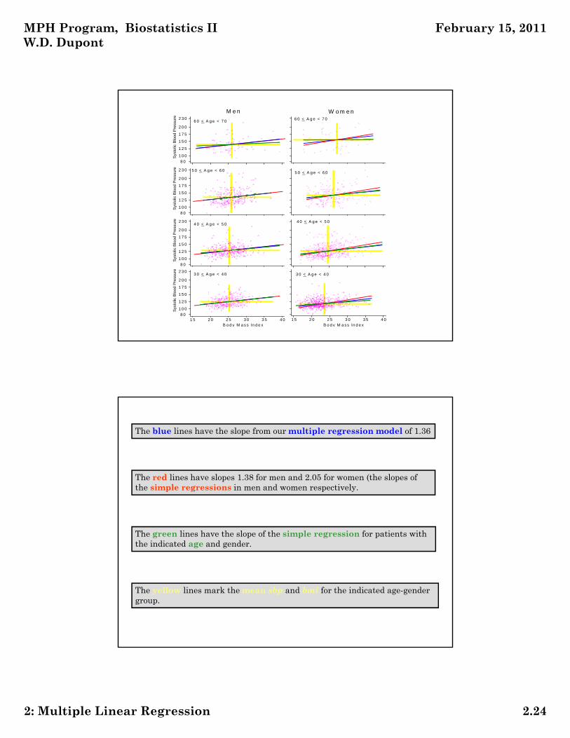
How reasonable is our model? One way to increase our intuitiveunderstanding of the model is to plot separate simple linear regressions ofsbp against bmi in groups of patients who are homogeneous with respect tothe other variables in the model. The following graphic is restricted topatients with a serum cholesterol of < 225 and subdivides patients by ageand sex. In these graphs, two versions of the graph are given drawn todifferent scales. The second only shows the regression lines.

Our multivariate model gives a single slope estimate of 1.36 for both sexes, but finds that the effect of increasing age on sbp is twice as large in women than men. I.e. For women this slope is 0.52 + 0.66 = 1.18 while for men it is 0.52.


February 15, 2011


B o d y M a s s In d e x1 5 2 0 2 5 3 0 3 5

Sys

tolic

Blo

od P

ress

ure

8 0

1 0 0

1 2 5

1 5 0

1 7 5

2 0 0

2 3 03 0 < A g e < 4 0

4 0

Sys

tolic

Blo

od P

ress

ure

8 0

1 0 0

1 2 5

1 5 0

1 7 5

2 0 0

2 3 04 0 < A g e < 5 0

Sys

tolic

Blo

od P

ress

ure

8 0

1 0 0

1 2 5

1 5 0

1 7 5

2 0 0

2 3 0S

ysto

lic B

loo

d P

ress

ure

8 0

1 0 0

1 2 5

1 5 0

1 7 5

2 0 0

2 3 06 0 < A g e < 7 0

M e n

5 0 < A g e < 6 0

W o m e n

4 0 < A g e < 5 0

5 0 < A g e < 6 0

6 0 < A g e < 7 0

B o d y M a s s In d e x1 5 2 0 2 5 3 0 3 5 4 0

3 0 < A g e < 4 0

The blue lines have the slope from our multiple regression model of 1.36

The red lines have slopes 1.38 for men and 2.05 for women (the slopes of the simple regressions in men and women respectively.

The green lines have the slope of the simple regression for patients with the indicated age and gender.

The yellow lines mark the mean sbp and bmi for the indicated age-gender group.


February 15, 2011


B ody M ass Index

Sys

tolic

Blo

od P

ress

ure

Sys

tolic

Blo

od P

ress

ure

4 0 < A ge < 50

Sys

tolic

Blo

od P

ress

ure

Sys

tolic

Blo

od P

ress

ure

6 0 < A ge < 70

M en

50 < A ge < 60

W om en

40 < A ge < 50

50 < A ge < 60

B ody M ass Index

30 < A ge < 4030 < A ge < 40

20 22 24 26 28 30 20 22 24 26 28 30100

110

120

130

140

150

160

100

110

120

130

140

150

160

100

110

120

130

140

150

160

100

110

120

130

140

150

160

60 < A ge < 70

For men the adjusted and unadjusted slopes are almost identical and are very close to the age restricted slope for all ages except 60 - 70.

However, for women the adjusted and unadjusted slopes differappreciably. The adjusted slope is very close to the age restricted slopes in every case except age 60 - 70, where the adjusted slope is closed the age restricted slope than is the unadjusted slope.

Thus, our model is a marked improvement over the simple model. The single sbp-bmi adjusted slope estimate appears reasonable except, for the oldest subjects.

Note that the mean sbp increases with age for both sexes, but increases more rapidly in women than in men.

The mean bmi does not vary appreciably with age in men but does increase with increasing age in women.

Thus age and gender confound the effect of bmi on sbp. Do you think that the age-gender interaction of sbp is real or is this driven by some other unknown confounding variable?


February 15, 2011


a) Forward Selection

i) Fit all simple linear models of y against each separate xvariable. Select the variable with the greatest significance.

10. Automatic Methods of Model Selection

Analyses loose power when we include variables in the model that are neither confounders nor variables of interest. When a large number of potential confounders are available it can be useful to use an automatic model selection program.

ii) Fit all possible models with the variable(s) selected in the preceding step(s) and one other. Select as the next variable the one with the greatest significance among these models.

iii) repeat step ii) to add additional variables, one variable at a time. Continue this process until none of the remaining variables have a significance level less than some threshold.

We next illustrate how this is done in Stata.

FramSBPbmiMulti.log continues as follows.

Source | SS df MS Number of obs = 4658-------------+------------------------------ F( 5, 4652) = 304.23

Model | 596342.421 5 119268.484 Prob > F = 0.0000Residual | 1823723.08 4652 392.029897 R-squared = 0.2464

-------------+------------------------------ Adj R-squared = 0.2456Total | 2420065.5 4657 519.661908 Root MSE = 19.8


-------------+----------------------------------------------------------------age | .5173521 .0517948 9.99 0.000 .4158098 .6188944bmi | 1.359621 .0734663 18.51 0.000 1.215592 1.50365scl | .0327898 .0069506 4.72 0.000 .0191632 .0464163

agewoman | .6646316 .0709159 9.37 0.000 .5256029 .8036603woman | -29.14655 3.316662 -8.79 0.000 -35.64878 -22.64432_cons | 65.74423 3.324712 19.77 0.000 59.22622 72.26224

------------------------------------------------------------------------------

. *

. * Fit a model of sbp against bmi age scl and sex with

. * interaction terms. The variables woman, bmiwoman,

. * agewoman, and sclwoman have been previously defined.

. *

. * statistics > other > stepwise estimation

. stepwise, pe(.1): regress sbp bmi age scl woman bmiwoman agewoman sclwoman{1}

begin with empty modelp = 0.0000 < 0.1000 adding age {2}p = 0.0000 < 0.1000 adding bmi {3}p = 0.0000 < 0.1000 adding sclp = 0.0001 < 0.1000 adding agewomanp = 0.0000 < 0.1000 adding woman


February 15, 2011


{1} Fit a model using forward selection; pe(.1) means that the Pvalue for entry is 0.1. At each step new variables will only beconsidered for entry into the model if their P value afteradjustment for previously entered variables is <0.1.

{2} In the first step the program considers the following models.sbp = 1 + bmi x 2

sbp = 1 + age x 2

sbp = 1 + scl x 2

sbp = 1 + woman x 2

sbp = 1 + bmiwoman x 2

sbp = 1 + agewoman x 2

sbp = 1 + sclwoman x 2

Of these models the one with age has the most significant slope parameter. The P value associated with this parameter is <0.1. Therefore we select age and go on to step 2.

{3} In step 2 we consider the models

sbp = 1 + age x 2 + bmi x 3

sbp = 1 + age x 2 + scl x 3

sbp = 1 + age x 2 + sclwoman x 3


February 15, 2011


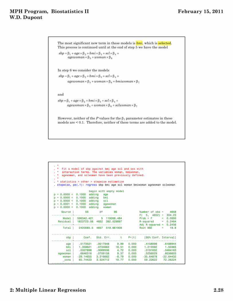
The most significant new term in these models is bmi, which is selected. This process is continued until at the end of step 5 we have the model

1 2 3 4sbp age bmi scl 5 6agewoman woman

1 2 3 4sbp age bmi scl

5 6 7agewoman woman bmiwoman

In step 6 we consider the models

and

1 2 3 4sbp age bmi scl

5 6 7agewoman woman sclwoman

However, neither of the P values for the 7 parameter estimates in these models are < 0.1. Therefore, neither of these terms are added to the model.

. *

. * Fit a model of sbp against bmi age scl and sex with

. * interaction terms. The variables woman, bmiwoman,

. * agewoman, and sclwoman have been previously defined.

. *


. stepwise, pe(.1): regress sbp bmi age scl woman bmiwoman agewoman sclwoman

begin with empty modelp = 0.0000 < 0.1000 adding agep = 0.0000 < 0.1000 adding bmip = 0.0000 < 0.1000 adding sclp = 0.0001 < 0.1000 adding agewomanp = 0.0000 < 0.1000 adding woman


Model | 596342.421 5 119268.484 Prob > F = 0.0000Residual | 1823723.08 4652 392.029897 R-squared = 0.2464

-------------+------------------------------ Adj R-squared = 0.2456Total | 2420065.5 4657 519.661908 Root MSE = 19.8


-------------+----------------------------------------------------------------age | .5173521 .0517948 9.99 0.000 .4158098 .6188944bmi | 1.359621 .0734663 18.51 0.000 1.215592 1.50365scl | .0327898 .0069506 4.72 0.000 .0191632 .0464163

agewoman | .6646316 .0709159 9.37 0.000 .5256029 .8036603woman | -29.14655 3.316662 -8.79 0.000 -35.64878 -22.64432_cons | 65.74423 3.324712 19.77 0.000 59.22622 72.26224

------------------------------------------------------------------------------


February 15, 2011


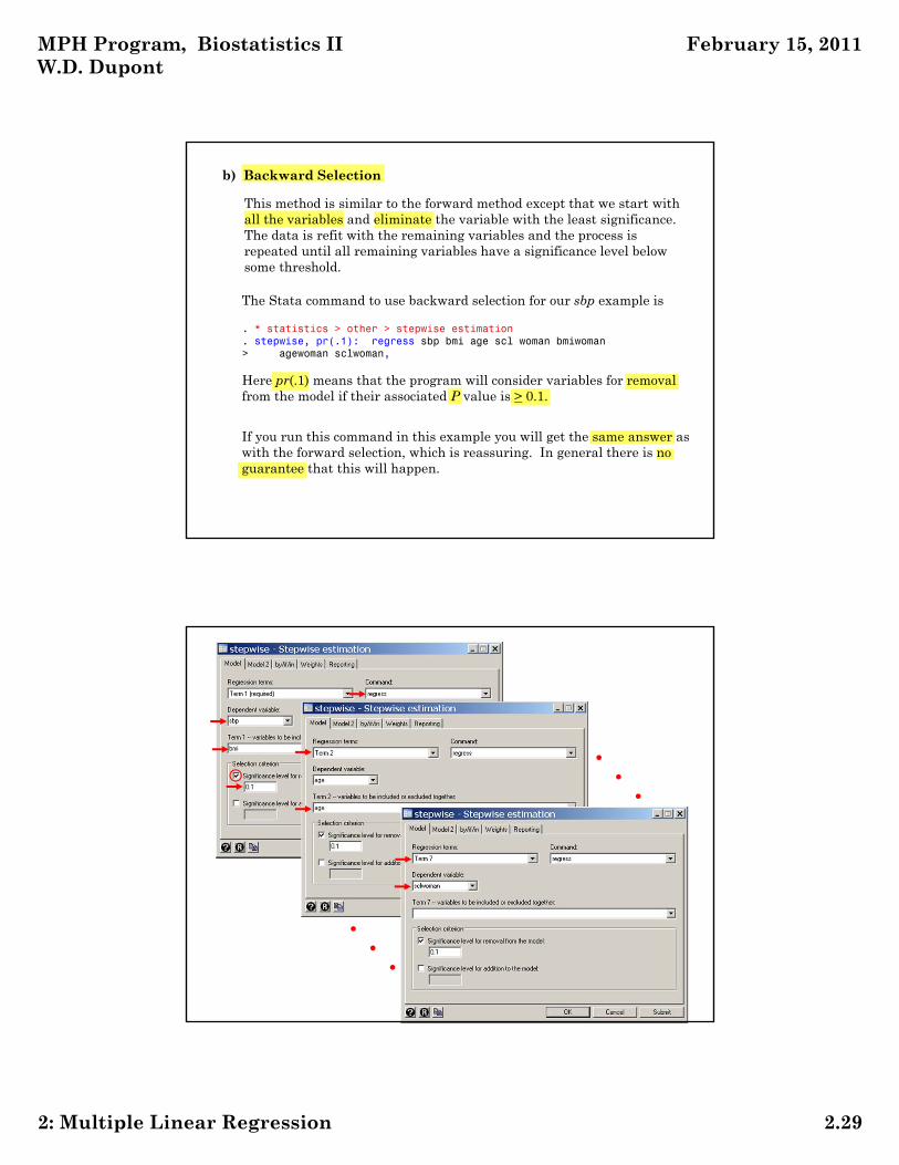
Here pr(.1) means that the program will consider variables for removal from the model if their associated P value is > 0.1.

b) Backward Selection

This method is similar to the forward method except that we start with all the variables and eliminate the variable with the least significance. The data is refit with the remaining variables and the process is repeated until all remaining variables have a significance level below some threshold.

The Stata command to use backward selection for our sbp example is


. stepwise, pr(.1): regress sbp bmi age scl woman bmiwoman > agewoman sclwoman,

If you run this command in this example you will get the same answer as with the forward selection, which is reassuring. In general there is no guarantee that this will happen.


February 15, 2011


c) Stepwise Selection

This method is like the forward method except that at each step,previously selected variables whose significance has dropped below somethreshold are dropped from the model.

Suppose:

x1 is the best single predictor of y

x2 and x3 are chosen next and together predict y better than x1

Then it makes sense to keep x2 and x3 and drop x1 from the model.

In the Stata stepwise command this is done with the options -,forward pe(.1) pr(.2)

which would consider new variables for selection with P < 0.1 and previously selected variables for removal with P > 0.2.

11. Pros and cons of automated model selection

iii) They can be misleading when used for exploratory analyses in which the primary variables of interest are unknown and the number of potential covariates is large. In this case these methods can exaggerate the importance of a small number of variables due to multiple comparisons artifacts.

iv) It is a good idea to use more than one method to see if you come up with the same model.

v) Fitting models by hand may sometimes be worth the effort.

i) Automatic selection methods are fast and easy to use.

ii) They are best used when we have a small number of variables of primary interest and wish to explore the effects of potential confounding variables on our models.


February 15, 2011


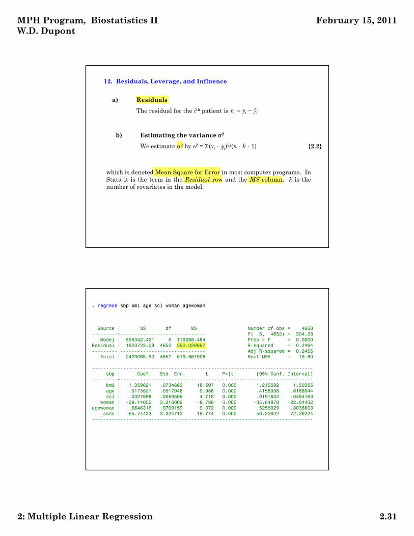
12. Residuals, Leverage, and Influence

î i ie y y

a) Residuals

The residual for the ith patient is

which is denoted Mean Square for Error in most computer programs. InStata it is the term in the Residual row and the MS column. k is thenumber of covariates in the model.

{2.2}y

b) Estimating the variance 2

We estimate 2 by s2 = (yi - i)2/(n - k - 1)

. regress sbp bmi age scl woman agewoman


Model | 596342.421 5 119268.484 Prob > F = 0.0000Residual | 1823723.08 4652 392.029897 R-squared = 0.2464 ---------+------------------------------ Adj R-squared = 0.2456

Total | 2420065.50 4657 519.661908 Root MSE = 19.80


---------+--------------------------------------------------------------------bmi | 1.359621 .0734663 18.507 0.000 1.215592 1.50365age | .5173521 .0517948 9.988 0.000 .4158098 .6188944scl | .0327898 .0069506 4.718 0.000 .0191632 .0464163

woman | -29.14655 3.316662 -8.788 0.000 -35.64878 -22.64432agewoman | .6646316 .0709159 9.372 0.000 .5256029 .8036603

_cons | 65.74423 3.324712 19.774 0.000 59.22622 72.26224------------------------------------------------------------------------------


February 15, 2011


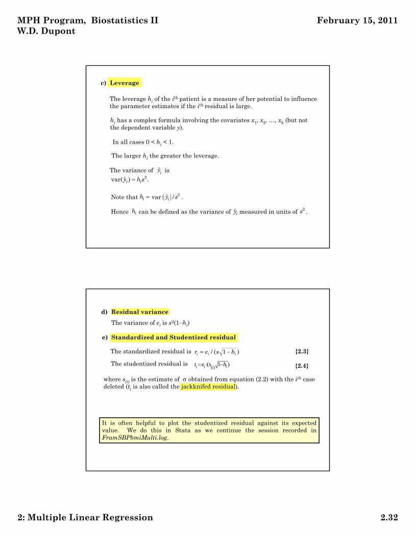
c) Leverage

The leverage hi of the ith patient is a measure of her potential to influence the parameter estimates if the ith residual is large.

hi has a complex formula involving the covariates x1, x2, …, xk (but not the dependent variable y).

The variance of i is y2var( ) .î iy h s

Note that var .

Hence can be defined as the variance of measured in units of .

ih 2/îy s

ih îy 2s

In all cases 0 < hi < 1.

The larger hi the greater the leverage.

d) Residual variance

The variance of ei is s2(1hi)

e) Standardized and Studentized residual

The standardized residual is {2.3}r e s hi i i / ( )1

The studentized residual is /( )

( 1 )ii i it e s h {2.4}

where s(i) is the estimate of obtained from equation (2.2) with the ith case deleted (ti is also called the jackknifed residual).

It is often helpful to plot the studentized residual against its expectedvalue. We do this in Stata as we continue the session recorded inFramSBPbmiMulti.log.


February 15, 2011


. predict yhat, xb(41 missing values generated)

. predict res, rstudent

. * Statistics > Nonparametric analysis > Lowess smoothing

. lowess res yhat, bwidth(0.2) symbol(oh) color(gs10) lwidth(thick) ///> yline(-1.96 0 1.96) ylabel(-2 (2) 6) ytick(-2 (1) 6) ///> xlabel(100 (20) 180) xtitle(Expected SBP)

-20

24

6S

tude

ntiz

ed re

sidu

als

100 120 140 160 180Expected SBP

bandwidth = .2

Lowess smoother


February 15, 2011


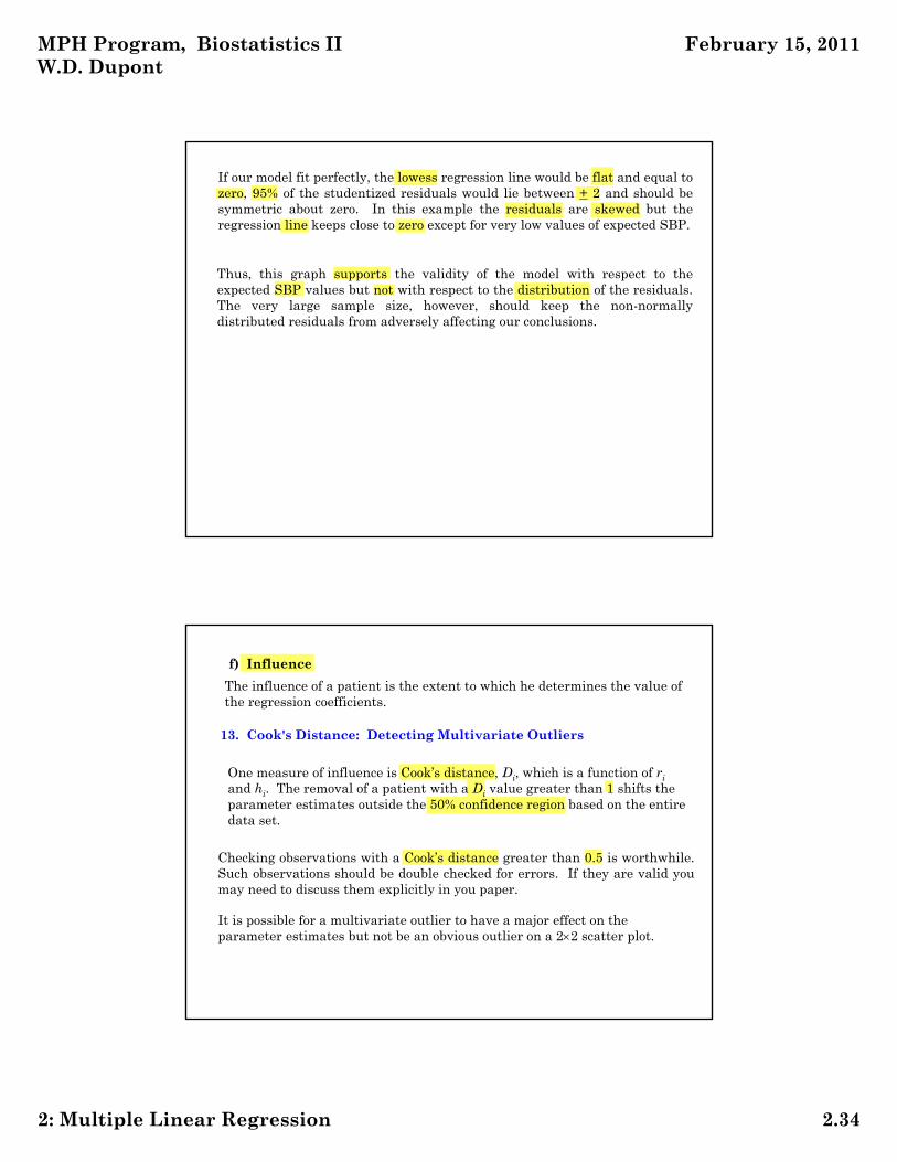
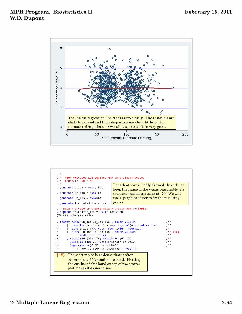
If our model fit perfectly, the lowess regression line would be flat and equal tozero, 95% of the studentized residuals would lie between + 2 and should besymmetric about zero. In this example the residuals are skewed but theregression line keeps close to zero except for very low values of expected SBP.

Thus, this graph supports the validity of the model with respect to theexpected SBP values but not with respect to the distribution of the residuals.The very large sample size, however, should keep the non-normallydistributed residuals from adversely affecting our conclusions.

f) Influence

The influence of a patient is the extent to which he determines the value of the regression coefficients.

13. Cook's Distance: Detecting Multivariate Outliers

One measure of influence is Cook’s distance, Di, which is a function of riand hi. The removal of a patient with a Di value greater than 1 shifts the parameter estimates outside the 50% confidence region based on the entire data set.

Checking observations with a Cook’s distance greater than 0.5 is worthwhile.Such observations should be double checked for errors. If they are valid youmay need to discuss them explicitly in you paper.

It is possible for a multivariate outlier to have a major effect on the parameter estimates but not be an obvious outlier on a 22 scatter plot.


February 15, 2011


. *

. * Illustrate influence of individual data points on

. * the parameter estimates of a linear regression.

. *

. * Variables Manager (right click on variable to be dropped or kept)

. drop res* Data > Create or change data > Keep or drop observations. keep if id > 2000 & id <= 2050(4649 observations deleted)

. regress sbp bmi age scl woman agewoman, level(50) {1}

14. Cook’s Distance in the SBP Regression Example

The Framingham data set is so large that no individual observation has an appreciable effect on the parameter estimates (the maximum Cook’s distance is 0.009). We illustrate the influence of individual patients in a subset analysis of subjects with IDs from 2001 to 2050. FramSBPbmiMulti.log continues as follows.

{1} The level(50) option specifies that 50% confidence intervals will be given for the parameter estimates.


February 15, 2011


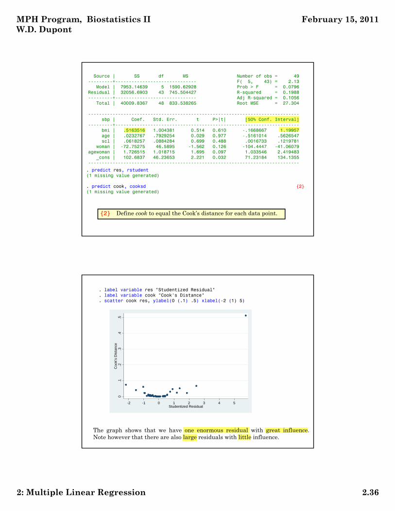
. predict res, rstudent(1 missing value generated)

. predict cook, cooksd {2}(1 missing value generated)



Total | 40009.8367 48 833.538265 Root MSE = 27.304


---------+--------------------------------------------------------------------bmi | .5163516 1.004381 0.514 0.610 -.1668667 1.19957age | .0232767 .7929254 0.029 0.977 -.5161014 .5626547scl | .0618257 .0884284 0.699 0.488 .0016733 .1219781

woman | -72.75275 46.5895 -1.562 0.126 -104.4447 -41.06079agewoman | 1.726515 1.018715 1.695 0.097 1.033546 2.419483

_cons | 102.6837 46.23653 2.221 0.032 71.23184 134.1355------------------------------------------------------------------------------

{2} Define cook to equal the Cook’s distance for each data point.

The graph shows that we have one enormous residual with great influence.Note however that there are also large residuals with little influence.

. label variable res "Studentized Residual"

. label variable cook "Cook's Distance"

. scatter cook res, ylabel(0 (.1) .5) xlabel(-2 (1) 5)

0.1

.2.3

.4.5

Coo

k's

Dis

tan

ce

-2 -1 0 1 2 3 4 5Studentized Residual


February 15, 2011


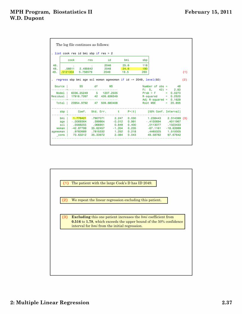
. list cook res id bmi sbp if res > 2

cook res id bmi sbp

46. . . 2046 25.6 118 48. .06611 2.485642 2048 24.6 190 49. .5121304 5.756579 2049 19.5 260 {1}

The log file continues as follows:

. regress sbp bmi age scl woman agewoman if id ~= 2049, level(50) {2}



Total | 23954.9792 47 509.680408 Root MSE = 20.655


---------+--------------------------------------------------------------------bmi | 1.776421 .7907071 2.247 0.030 1.238443 2.314399 {3}age | -.0069364 .599864 -0.012 0.991 -.4150694 .4011967scl | .0568255 .066901 0.849 0.400 .0113077 .1023433

woman | -42.87799 35.62457 -1.204 0.235 -67.1161 -18.63989agewoman | .9782689 .7815332 1.252 0.218 .4465325 1.510005

_cons | 73.63212 35.33972 2.084 0.043 49.58782 97.67642------------------------------------------------------------------------------

{1} The patient with the large Cook’s D has ID 2049.

{2} We repeat the linear regression excluding this patient.

{3} Excluding this one patient increases the bmi coefficient from 0.516 to 1.78, which exceeds the upper bound of the 50% confidence interval for bmi from the initial regression.


February 15, 2011




Total | 40009.8367 48 833.538265 Root MSE = 27.304


---------+--------------------------------------------------------------------bmi | .5163516 1.004381 0.514 0.610 -.1668667 1.19957age | .0232767 .7929254 0.029 0.977 -.5161014 .5626547scl | .0618257 .0884284 0.699 0.488 .0016733 .1219781

woman | -72.75275 46.5895 -1.562 0.126 -104.4447 -41.06079agewoman | 1.726515 1.018715 1.695 0.097 1.033546 2.419483

_cons | 102.6837 46.23653 2.221 0.032 71.23184 134.1355------------------------------------------------------------------------------

. regress sbp bmi age scl woman agewoman, level(50)

The following graph shows a scatter plot of sbp by bmi for these 50 patients.The red and blue lines have slopes of 1.78 and 0.516, respectively (the linesare drawn through the mean sbp and bmi values). Patients 2048 and 2049are indicated by arrows. The influence of patient 2048 is greatly reduced bythe fact that his bmi of 24.6 is near the mean bmi. The influence of patient2049 is not only affected by her large residual but also by her low bmi thatexerts leverage on the regression slope.

2000 < id < 2051

Sys

tolic

Blo

od P

ress

ure

Body Mass Index20 25 30 35

100

150

200

250 Enormous residualwith great influence

Large residualwith little influence


February 15, 2011


15. Least Squares Estimation

In simple linear regression we have introduced the concept of estimating parameters by the method of least squares.

We chose a model of the form E(yi) = + xi.

We estimated by a and by b letting

and then choosing a and b so as to minimize y = a + bx

2ˆy y the sum of squared residuals

This approach works well for linear regression. It is ineffective for some other regression methods

Another approach which can be very useful ismaximum likelihood estimation

16. Maximum Likelihood Estimation

In simple linear regression we observed pairs of observations

and fit the model E(yi) = + xi , : 1,2, ,i iy x i n

We calculate the likelihood function

which is the probability of obtaining the observed data given the specified value of and .

The maximum likelihood estimates of and are those values of these parameters that maximize equation {1}

In linear regression the maximum likelihood and least squares estimates of and are identical.

L , | , : 1,2, ,i iy x i n {1}


February 15, 2011


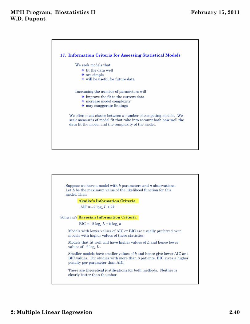
17. Information Criteria for Assessing Statistical Models

fit the data well are simple will be useful for future data

We seek models that

improve the fit to the current data increase model complexity may exaggerate findings

Increasing the number of parameters will

We often must choose between a number of competing models. We seek measures of model fit that take into account both how well the data fit the model and the complexity of the model.

Models with lower values of AIC or BIC are usually preferred over models with higher values of these statistics.

Schwarz’s Bayesian Information Criteria

BIC = 2 loge L + k loge n

Suppose we have a model with k parameters and n observations. Let L be the maximum value of the likelihood function for this model. Then

Akaike’s Information Criteria

AIC = 2 loge L + 2k

Models that fit well will have higher values of L and hence lower values of 2 loge L .

Smaller models have smaller values of k and hence give lower AIC and BIC values. For studies with more than 8 patients, BIC gives a higher penalty per parameter than AIC.

There are theoretical justifications for both methods. Neither is clearly better than the other.


February 15, 2011


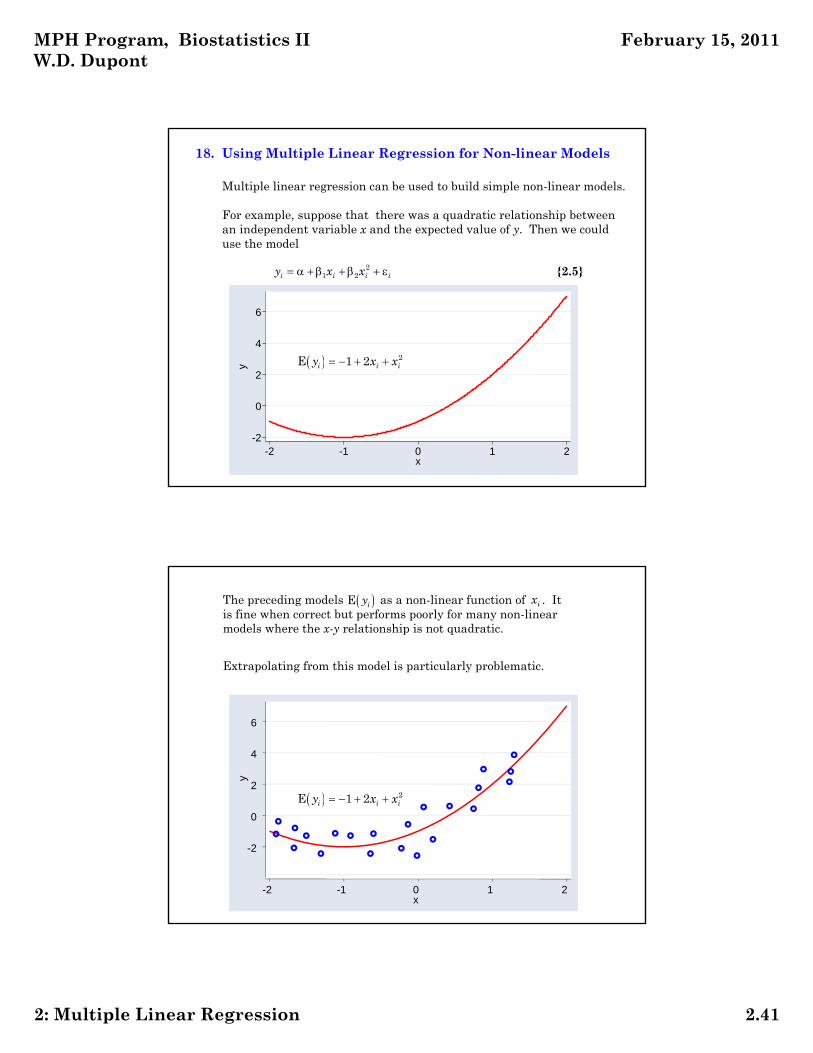
Multiple linear regression can be used to build simple non-linear models.

For example, suppose that there was a quadratic relationship between an independent variable x and the expected value of y. Then we could use the model

21 2i i i iy x x {2.5}

-2

0

2

4

6

y

-2 -1 0 1 2x

2E 1 2i i iy x x

18. Using Multiple Linear Regression for Non-linear Models

The preceding models as a non-linear function of . It is fine when correct but performs poorly for many non-linear models where the x-y relationship is not quadratic.

E iy ix

-2

0

2

4

6

y

-2 -1 0 1 2x

2E 1 2i i iy x x

Extrapolating from this model is particularly problematic.


February 15, 2011


Note that {2.5} is a linear function of the parameters. Hence, it is a multiple linear regression model even though it is non-linear in ix

-2

0

2

4

6

y

-2 -1 0 1 2x

21 2i i i iy x x

We seek a more flexible approach to building non-linear regression models using multiple linear regression models.

19. Restricted Cubic Splines

We wish to model yi as a function of xi using a flexible non-linear model.In a restricted cubic spline model we introduce k knots on the x-axis located at . We select a model of the expected value of y that 1 2, , , kt t t

is linear before and after . 1t kt

consists of piecewise cubic polynomials between adjacent knots(i.e. of the form ) 3 2ax bx cx d

is continuous and smooth at each knot. (More technically, its first and second derivatives are continuous at each knot.)

An example of a restricted cubic spline with three knots is given on the next slide.


February 15, 2011


1t 2t 3t

Example of a restricted cubic spline with three knots

Given x and k knots, a restricted cubic spline can be defined by

1 1 2 2 1 1k ky x x x

for suitably defined values of ix

These covariates are functions of x and the knots but are independent of y.

1x x and hence the hypothesistests the linear hypothesis.

2 3 1 0k

Programs to calculate are available in Stata, R and other statistical software packages. The functional definitions of these terms are not pretty (see Harrell 2001), but this is of little concern given programs that will calculate them for you.

1 1, , kx x

Users can specify the knot values. However, it is often reasonable to let you program choose them for you.

If x is less than the first knot then This fact will prove useful in survival analyses when calculating relative risks.

2 3 1 0kx x x


February 15, 2011


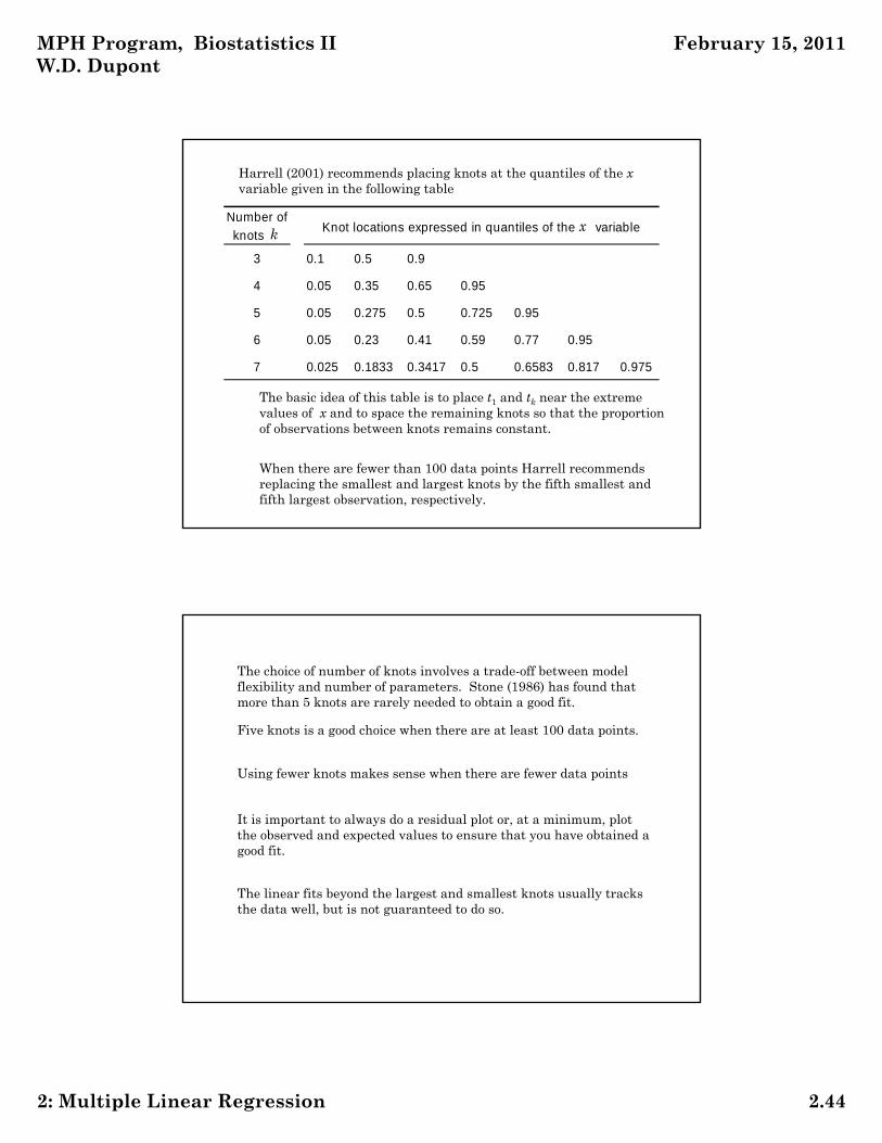
Harrell (2001) recommends placing knots at the quantiles of the x variable given in the following table

Number of

knots k

3 0.1 0.5 0.9

4 0.05 0.35 0.65 0.95

5 0.05 0.275 0.5 0.725 0.95

6 0.05 0.23 0.41 0.59 0.77 0.95

7 0.025 0.1833 0.3417 0.5 0.6583 0.817 0.975

Knot locations expressed in quantiles of the x variable

The basic idea of this table is to place t1 and tk near the extreme values of x and to space the remaining knots so that the proportion of observations between knots remains constant.

When there are fewer than 100 data points Harrell recommends replacing the smallest and largest knots by the fifth smallest and fifth largest observation, respectively.

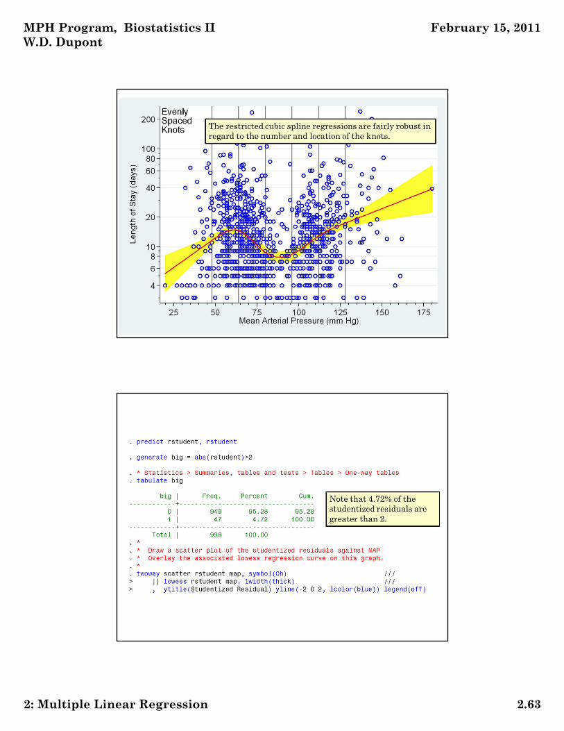
The choice of number of knots involves a trade-off between model flexibility and number of parameters. Stone (1986) has found that more than 5 knots are rarely needed to obtain a good fit.

Five knots is a good choice when there are at least 100 data points.

Using fewer knots makes sense when there are fewer data points

It is important to always do a residual plot or, at a minimum, plot the observed and expected values to ensure that you have obtained a good fit.

The linear fits beyond the largest and smallest knots usually tracks the data well, but is not guaranteed to do so.


February 15, 2011


20. Example: the SUPPORT Study

A prospective observational study of hospitalized patients

los = length of stay in days.

map = baseline mean arterial pressure

1: Patient died in hospital

0: Patient discharged alive

fate =

Lynn & Knauss: "Background for SUPPORT." J Clin Epidemiol 1990; 43: 1S - 4S.

A random sample of data from 996 subjects in this study is available. See

3.25.2.SUPPORT.dta

0

25

50

75

100

125

150

175

200

225

Len

gth

of S

tay

(da

ys)

25 50 75 100 125 150 175Mean Arterial Pressure (mm Hg)


February 15, 2011


21. Fitting a Restricted Cubic Spline with Stata

. * SupportLinearRCS.log

. *

. * Draw scatter plots of length-of-stay (LOS) by mean arterial

. * pressure (MAP) and log LOS by MAP for the SUPPORT Study data

. * (Lynn & Knauss, 1990).

. *

. use "C:\WDDtext\3.25.2.SUPPORT.dta" , replace

. scatter los map, symbol(Oh) xlabel(25 (25) 175) xmtick(20 (5) 180) /// {1}> ylabel(0(25)225, angle(0)) ymtick(5(5)240)

{1} Length of stay is highly skewed.

0

25

50

75

100

125

150

175

200

225

Len

gth

of S

tay

(da

ys)



February 15, 2011


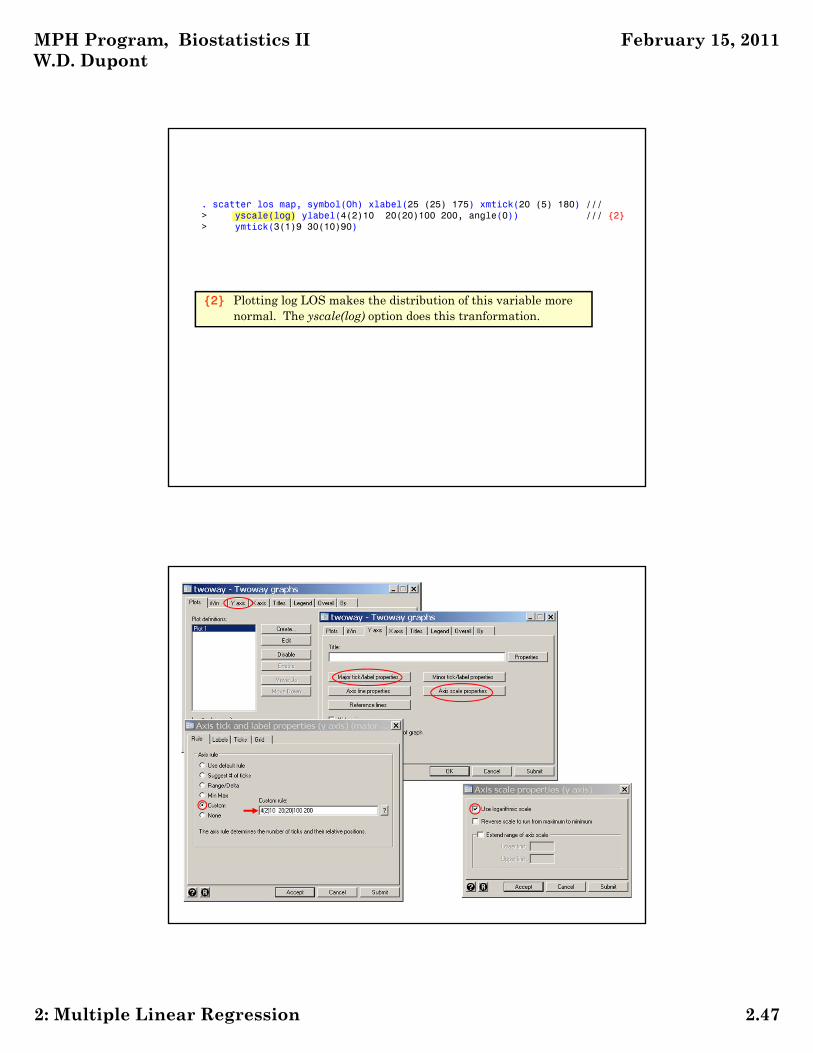
. scatter los map, symbol(Oh) xlabel(25 (25) 175) xmtick(20 (5) 180) ///> yscale(log) ylabel(4(2)10 20(20)100 200, angle(0)) /// {2}> ymtick(3(1)9 30(10)90)

{2} Plotting log LOS makes the distribution of this variable more normal. The yscale(log) option does this tranformation.


February 15, 2011


4

6

810

20

40

60

80100

200

Len

gth

of S

tay

(da

ys)


. *

. * Regress log LOS against MAP using RCS models with

. * 5 knots at their default locations. Overlay the expected

. * log LOS from these models on a scatter plot of log LOS by MAP.

. *

. * Data > Create... > Other variable-creation... > linear and cubic...mkspline _Smap = map, cubic displayknots {1}

| knot1 knot2 knot3 knot4 knot5 -------------+-------------------------------------------------------

map | 47 66 78 106 129

The mkspline command generates either linear or restricted cubic spline covariates. The cubic option specifies that restricted cubic spline covariates are to be created. This command generates these covariates for the variable map. By default, 5 knots are used at their default locations. Following Harrell's recommendation the computer placesthem at the 5th, 27.5th, 50th, 72.5th and 95th percentiles of map. The values of these knots are listed.

The 4 spline covariates associated with these 5 knots are named_Smap1_Smap2_Smap3_Smap4

These names are obtained by concatenating the name _Smap givenbefore the equal sign with the numbers 1, 2, 3 and 4.

{1}


February 15, 2011


. summarize _Smap1 _Smap2 _Smap3 _Smap4 {2}

Variable | Obs Mean Std. Dev. Min Max-------------+--------------------------------------------------------

_Smap1 | 996 85.31727 26.83566 20 180_Smap2 | 996 20.06288 27.34701 0 185.6341_Smap3 | 996 7.197497 11.96808 0 89.57169_Smap4 | 996 3.121013 5.96452 0 48.20881

{2} _Smap1 is identical to map. The other spline covariates take non-negative values.


February 15, 2011


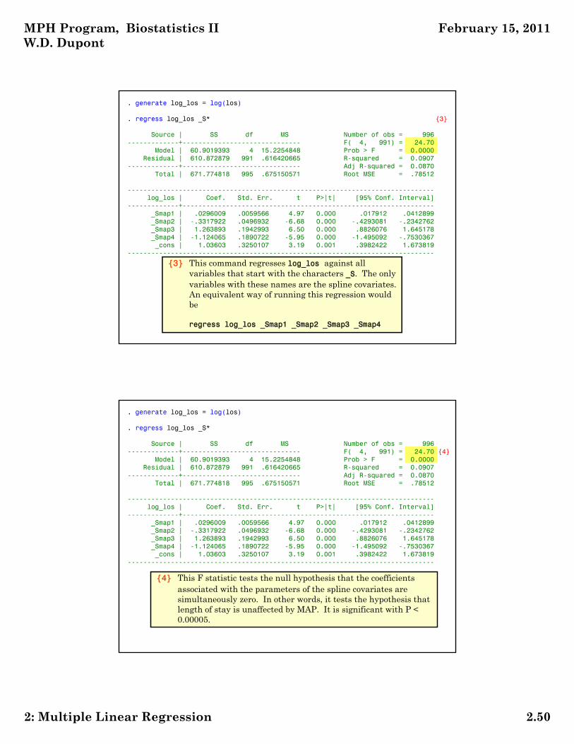
. generate log_los = log(los)

. regress log_los _S* {3}


Model | 60.9019393 4 15.2254848 Prob > F = 0.0000Residual | 610.872879 991 .616420665 R-squared = 0.0907

-------------+------------------------------ Adj R-squared = 0.0870Total | 671.774818 995 .675150571 Root MSE = .78512

------------------------------------------------------------------------------log_los | Coef. Std. Err. t P>|t| [95% Conf. Interval]

-------------+----------------------------------------------------------------_Smap1 | .0296009 .0059566 4.97 0.000 .017912 .0412899_Smap2 | -.3317922 .0496932 -6.68 0.000 -.4293081 -.2342762_Smap3 | 1.263893 .1942993 6.50 0.000 .8826076 1.645178_Smap4 | -1.124065 .1890722 -5.95 0.000 -1.495092 -.7530367_cons | 1.03603 .3250107 3.19 0.001 .3982422 1.673819

------------------------------------------------------------------------------{3} This command regresses log_los against all

variables that start with the characters _S. The only variables with these names are the spline covariates. An equivalent way of running this regression would be

regress log_los _Smap1 _Smap2 _Smap3 _Smap4

. generate log_los = log(los)

. regress log_los _S*

Source | SS df MS Number of obs = 996-------------+------------------------------ F( 4, 991) = 24.70 {4}




-------------+----------------------------------------------------------------_Smap1 | .0296009 .0059566 4.97 0.000 .017912 .0412899_Smap2 | -.3317922 .0496932 -6.68 0.000 -.4293081 -.2342762_Smap3 | 1.263893 .1942993 6.50 0.000 .8826076 1.645178_Smap4 | -1.124065 .1890722 -5.95 0.000 -1.495092 -.7530367_cons | 1.03603 .3250107 3.19 0.001 .3982422 1.673819

------------------------------------------------------------------------------

{4} This F statistic tests the null hypothesis that the coefficients associated with the parameters of the spline covariates are simultaneously zero. In other words, it tests the hypothesis that length of stay is unaffected by MAP. It is significant with P < 0.00005.


February 15, 2011


* Statistics > Postestimation > Reports and statistics. estat ic {5}

-----------------------------------------------------------------------------Model | Obs ll(null) ll(model) df AIC BIC

-------------+---------------------------------------------------------------. | 996 -1217.138 -1169.811 5 2349.623 2374.141

-----------------------------------------------------------------------------Note: N=Obs used in calculating BIC; see [R] BIC note

{5} Calculate the AIC and BIC for this model.

. * Statistics > Postestimation > Tests > Test linear hypotheses

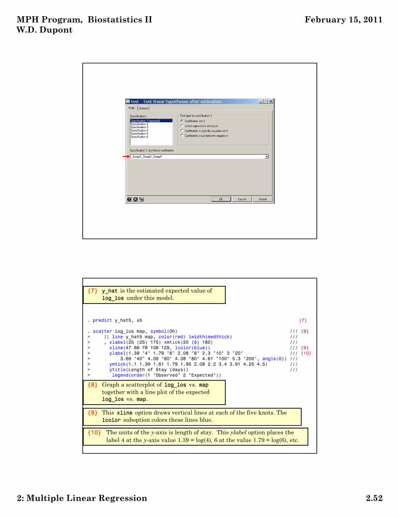
. test _Smap2 _Smap3 _Smap4 {6}

( 1) _Smap2 = 0( 2) _Smap3 = 0( 3) _Smap4 = 0

F( 3, 991) = 30.09Prob > F = 0.0000

{6} Test the null hypothesis that there is a linear relationship between map andlog_los. Since _Smap1 = map, this is done by testing the null hypothesis that the coefficients associated with _Smap2, _Smap3and _Smap4 are all simultaneously zero.This test is significant with P < 0.00005.


February 15, 2011


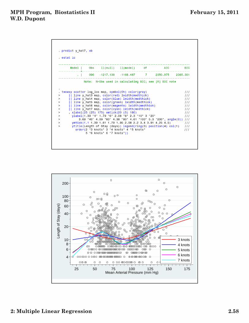
. predict y_hat5, xb {7}

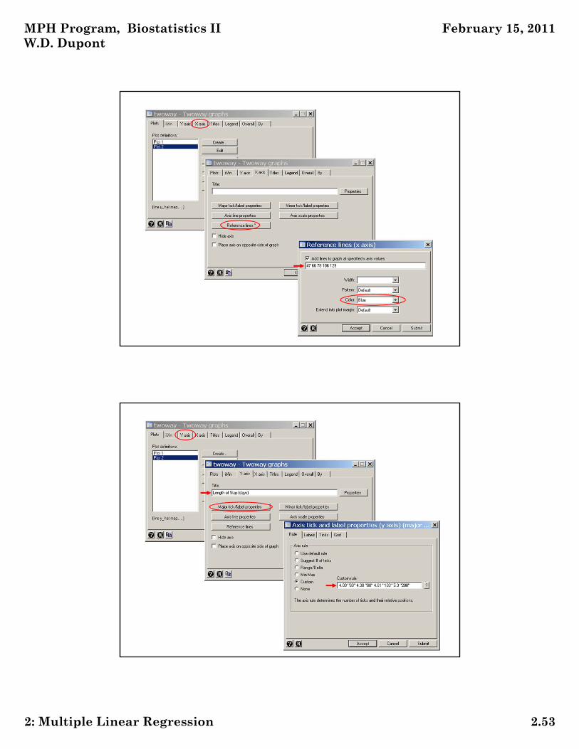
. scatter log_los map, symbol(Oh) /// {8}> || line y_hat5 map, color(red) lwidth(medthick) ///> , xlabel(25 (25) 175) xmtick(20 (5) 180) ///> xline(47 66 78 106 129, lcolor(blue)) /// {9}> ylabel(1.39 "4" 1.79 "6" 2.08 "8" 2.3 "10" 3 "20" /// {10}> 3.69 "40" 4.09 "60" 4.38 "80" 4.61 "100" 5.3 "200", angle(0)) ///> ymtick(1.1 1.39 1.61 1.79 1.95 2.08 2.2 3.4 3.91 4.25 4.5) ///> ytitle(Length of Stay (days)) ///> legend(order(1 "Observed" 2 "Expected"))

{7} y_hat is the estimated expected value oflog_los under this model.

{8} Graph a scatterplot of log_los vs. maptogether with a line plot of the expectedlog_los vs. map.

{9} This xline option draws vertical lines at each of the five knots. Thelcolor suboption colors these lines blue.

{10} The units of the y-axis is length of stay. This ylabel option places the label 4 at the y-axis value 1.39 = log(4), 6 at the value 1.79 = log(6), etc.


February 15, 2011



February 15, 2011


4

68

10

20

40

6080

100

200

Len

gth

of S

tay

(da

ys)


Observed Expected

. *

. * Plot expected LOS for models with 3, 4, 6 and 7 knots.

. * Use the default knot locations. Calculate AIC and BIC for each model.

. *

. * Variables Manager

. drop _S*

. * Data > Create... > Other variable-creation... > linear and cubic...

. mkspline _Smap = map, nknots(3) cubic displayknots {11}

| knot1 knot2 knot3 -------------+---------------------------------

map | 55 78 120

{11} Define 2 spline covariates associated with 3 knots at their default locations. The nknots option specifies the number of knots.


February 15, 2011







-------------+----------------------------------------------------------------_Smap1 | -.0110138 .0027449 -4.01 0.000 -.0164002 -.0056274_Smap2 | .0226496 .004248 5.33 0.000 .0143135 .0309858_cons | 3.124095 .1827706 17.09 0.000 2.765435 3.482756

------------------------------------------------------------------------------

. predict y_hat3, xb

. estat ic


-------------+---------------------------------------------------------------. | 996 -1217.138 -1199.17 3 2404.34 2419.051



February 15, 2011


. drop _S*

. mkspline _Smap = map, nknots(4) cubic displayknots

| knot1 knot2 knot3 knot4 -------------+--------------------------------------------

map | 47 69 100 129






-------------+----------------------------------------------------------------_Smap1 | .0060744 .004387 1.38 0.166 -.0025343 .0146832_Smap2 | -.0533119 .0155968 -3.42 0.001 -.0839184 -.0227054_Smap3 | .1509453 .0342118 4.41 0.000 .0838095 .2180812_cons | 2.180462 .2600792 8.38 0.000 1.670093 2.69083

------------------------------------------------------------------------------

. predict y_hat4, xb

. estat ic


-------------+---------------------------------------------------------------. | 996 -1217.138 -1185.913 4 2379.827 2399.442


. drop _S*

. mkspline _Smap = map, nknots(6) cubic displayknots

| knot1 knot2 knot3 knot4 knot5 knot6 -------------+------------------------------------------------------------------

map | 47 63 73 93 108.69 129


February 15, 2011







-------------+----------------------------------------------------------------_Smap1 | .03099 .006904 4.49 0.000 .0174418 .0445382_Smap2 | -.3837563 .0874071 -4.39 0.000 -.5552809 -.2122318_Smap3 | 1.111961 .3834093 2.90 0.004 .3595729 1.864349_Smap4 | -.5873248 .4457995 -1.32 0.188 -1.462145 .2874957_Smap5 | -.4824613 .2991149 -1.61 0.107 -1.069433 .1045108_cons | .9745223 .3623654 2.69 0.007 .2634297 1.685615

------------------------------------------------------------------------------. predict y_hat6, xb

. estat ic


-------------+---------------------------------------------------------------. | 996 -1217.138 -1168.809 6 2349.618 2379.04



February 15, 2011


4

6

810

20

40

60

80100

200

Len

gth

of S

tay

(da

ys)


3 knots

4 knots5 knots6 knots

7 knots


February 15, 2011



February 15, 2011



February 15, 2011


4

6

810

20

40

60

80100

200

Len

gth

of S

tay

(da

ys)


EvenlySpacedKnots


February 15, 2011


4

6

810

20

40

60

80100

200

Len

gth

of S

tay

(da

ys)


DefaultKnotValues


February 15, 2011



February 15, 2011



February 15, 2011


0

10

20

30

40

50

60

70L

engt

h of

Sta

y


Expected MAP 95% Confidence Interval

> 70


February 15, 2011


Cited References

Levy D, National Heart Lung and Blood Institute., Center for Bio-Medical Communication. 50 Years of Discovery : Medical Milestones from the National Heart, Lung, and Blood Institute's Framingham Heart Study.Hackensack, N.J.: Center for Bio-Medical Communication Inc.; 1999.

Knaus,W.A., Harrell, F.E., Jr., Lynn, J., Goldman, L., Phillips, R.S., Connors, A.F., Jr. et al. The SUPPORT prognostic model. Objective estimates of survival for seriously ill hospitalized adults. Study to understand prognoses and preferences for outcomes and risks of treatments. Ann Intern Med. 1995; 122:191-203.

For additional references on these notes see.

Dupont WD. Statistical Modeling for Biomedical Researchers: A Simple Introduction to the Analysis of Complex Data. 2nd ed. Cambridge, U.K.: Cambridge University Press; 2009.

MPH Program, Biostatistics II February 15, 2011 W.D. Dupontbiostat.mc.vanderbilt.edu/wiki/pub/Main/BiostatIILectureNotes/02... · MPH Program, Biostatistics II W.D. Dupont February

Documents