MPEG-4 and Rate-Distortion-Based Shape-Coding Techniques AGGELOS K. KATSAGGELOS, FELLOW, IEEE, LISIMACHOS P. KONDI, STUDENT MEMBER, IEEE, FABIAN W. MEIER, J ¨ ORN OSTERMANN, AND GUIDO M. SCHUSTER, MEMBER, IEEE In this paper, we address the problem of the efficient encoding of object boundaries. This problem is becoming increasingly impor- tant in applications such as content-based storage and retrieval, studio and television postproduction, and mobile multimedia appli- cations. The MPEG-4 visual standard will allow the transmission of arbitrarily shaped video objects. The techniques developed for shape coding within the MPEG-4 standardization effort are de- scribed and compared first. A framework for the representation of shapes using their contours is presented next. Such representations are achieved using curves of various orders, and they are optimal in the rate-distortion sense. Last, conclusions are drawn. Keywords—Boundary coding, MPEG-4, rate-distortion theory, shape coding, video coding. I. INTRODUCTION With video being a ubiquitous part of modern multimedia communications, new functionalities in addition to the con- ventional compression provided by existing video-coding standards like H.261, MPEG-1, H.262, MPEG-2, and H.263 are required for new applications. Applications like digital libraries or content-based storage and retrieval have to allow access to video data based on object descriptions, where objects are described by texture, shape, and motion. Studio and television postproduction applications require editing of video content with objects represented by texture and shape. For collaborative scene visualization like augmented reality, we want to place video objects into the scene. Mobile multimedia applications require content-based interactivity and content-based scalability in order to allocate a limited bit rate to different semantic parts of a scene and to fit the individual needs. All these applications share one common Manuscript received August 30, 1997; revised December 15, 1997. The Guest Editor coordinating the review of this paper and approving it for publication was K. J. R. Liu. A. K. Katsaggelos and L. P. Kondi are with the Department of Electrical and Computer Engineering, Northwestern University, Evanston, IL 60208- 3118 USA. F. W. Meier is with Silicon Graphics, Mountain View, CA 94043-1389 USA. J. Ostermann is with AT&T Labs-Research, Red Bank, NJ 07701-7033 USA. G. M. Schuster is with 3Com, Mount Prospect, IL 60016 USA. Publisher Item Identifier S 0018-9219(98)03521-X. requirement: video content has to be easily accessible on an object basis. Given the application requirements, video objects have to be described not only by texture but also by shape. The importance of shape for video objects has been realized early on by the broadcast and movie industry by employing the so-called chroma-keying technique. Coding algorithms like object-based analysis-synthesis coding [1] use shape as a parameter in addition to texture and motion for describing moving video objects. Second-generation image coding segments an image into regions and describes each region by texture and shape [2]. The purpose of using shape was to achieve better subjective picture quality, increased coding efficiency as well as an object-based video representation. MPEG-4 visual will be the first international standard allowing the transmission of arbitrarily shaped video objects (VO’s) [3]. A frame of a VO is called a video object plane (VOP). Following an object-based approach, MPEG-4 vi- sual transmits texture, motion, and shape information of one VO within one bitstream. The bitstreams of several VO’s and accompanying composition information can be multi- plexed such that the decoder receives all the information to decode the VO’s and arrange them into a video scene. This results in a new dimension of interactivity and flexibility for standardized video and multimedia applications. After a review of object-based coders and shape cod- ing (Section II), this paper provides an overview of the main algorithms for shape, as investigated within MPEG- 4, in Section III. Two types of VO’s are distinguished. For opaque objects, binary shape information is transmit- ted. Two bitmap-based (Section III-A), two contour-based (Section III-B), and an implicit shape coder (Section III- C) are presented. The evaluation criteria for measuring coding performance and the test sequences are discussed in Section III-D. The performance of the five shape coders, verified by bitstream exchange, in terms of coding effi- ciency, error resilience, and hardware implementation is compared in Section III-E. Transparent objects are de- scribed by grayscale -maps (8 bits/pel) defining the outline as well as the transparency of an object (Section III-F). 0018–9219/98$10.00 1998 IEEE 1126 PROCEEDINGS OF THE IEEE, VOL. 86, NO. 6, JUNE 1998

Welcome message from author
This document is posted to help you gain knowledge. Please leave a comment to let me know what you think about it! Share it to your friends and learn new things together.
Transcript

MPEG-4 and Rate-Distortion-BasedShape-Coding Techniques
AGGELOS K. KATSAGGELOS,FELLOW, IEEE, LISIMACHOS P. KONDI, STUDENT MEMBER, IEEE,FABIAN W. MEIER, JORN OSTERMANN,AND GUIDO M. SCHUSTER,MEMBER, IEEE
In this paper, we address the problem of the efficient encoding ofobject boundaries. This problem is becoming increasingly impor-tant in applications such as content-based storage and retrieval,studio and television postproduction, and mobile multimedia appli-cations. The MPEG-4 visual standard will allow the transmissionof arbitrarily shaped video objects. The techniques developed forshape coding within the MPEG-4 standardization effort are de-scribed and compared first. A framework for the representation ofshapes using their contours is presented next. Such representationsare achieved using curves of various orders, and they are optimalin the rate-distortion sense. Last, conclusions are drawn.
Keywords—Boundary coding, MPEG-4, rate-distortion theory,shape coding, video coding.
I. INTRODUCTION
With video being a ubiquitous part of modern multimediacommunications, new functionalities in addition to the con-ventional compression provided by existing video-codingstandards like H.261, MPEG-1, H.262, MPEG-2, and H.263are required for new applications. Applications like digitallibraries or content-based storage and retrieval have to allowaccess to video data based on object descriptions, whereobjects are described by texture, shape, and motion. Studioand television postproduction applications require editing ofvideo content with objects represented by texture and shape.For collaborative scene visualization like augmented reality,we want to place video objects into the scene. Mobilemultimedia applications require content-based interactivityand content-based scalability in order to allocate a limitedbit rate to different semantic parts of a scene and to fit theindividual needs. All these applications share one common
Manuscript received August 30, 1997; revised December 15, 1997. TheGuest Editor coordinating the review of this paper and approving it forpublication was K. J. R. Liu.
A. K. Katsaggelos and L. P. Kondi are with the Department of Electricaland Computer Engineering, Northwestern University, Evanston, IL 60208-3118 USA.
F. W. Meier is with Silicon Graphics, Mountain View, CA 94043-1389USA.
J. Ostermann is with AT&T Labs-Research, Red Bank, NJ 07701-7033USA.
G. M. Schuster is with 3Com, Mount Prospect, IL 60016 USA.Publisher Item Identifier S 0018-9219(98)03521-X.
requirement: video content has to be easily accessible onan object basis.
Given the application requirements, video objects haveto be described not only by texture but also by shape. Theimportance of shape for video objects has been realizedearly on by the broadcast and movie industry by employingthe so-called chroma-keying technique. Coding algorithmslike object-based analysis-synthesis coding [1] use shape asa parameter in addition to texture and motion for describingmoving video objects. Second-generation image codingsegments an image into regions and describes each regionby texture and shape [2]. The purpose of using shape was toachieve better subjective picture quality, increased codingefficiency as well as an object-based video representation.
MPEG-4 visual will be the first international standardallowing the transmission of arbitrarily shaped video objects(VO’s) [3]. A frame of a VO is called a video object plane(VOP). Following an object-based approach, MPEG-4 vi-sual transmits texture, motion, and shape information of oneVO within one bitstream. The bitstreams of several VO’sand accompanying composition information can be multi-plexed such that the decoder receives all the information todecode the VO’s and arrange them into a video scene. Thisresults in a new dimension of interactivity and flexibilityfor standardized video and multimedia applications.
After a review of object-based coders and shape cod-ing (Section II), this paper provides an overview of themain algorithms for shape, as investigated within MPEG-4, in Section III. Two types of VO’s are distinguished.For opaque objects, binary shape information is transmit-ted. Two bitmap-based (Section III-A), two contour-based(Section III-B), and an implicit shape coder (Section III-C) are presented. The evaluation criteria for measuringcoding performance and the test sequences are discussedin Section III-D. The performance of the five shape coders,verified by bitstream exchange, in terms of coding effi-ciency, error resilience, and hardware implementation iscompared in Section III-E. Transparent objects are de-scribed by grayscale-maps (8 bits/pel) defining the outlineas well as the transparency of an object (Section III-F).
0018–9219/98$10.00 1998 IEEE
1126 PROCEEDINGS OF THE IEEE, VOL. 86, NO. 6, JUNE 1998

In Section IV, contour-based coding is revisited. Aframework is presented for obtaining optimal lossyencoding results in the operational rate-distortion sense(Section IV-A). In Section IV-B, different distortionmeasures that can be used in boundary encoding aredescribed. In Section IV-C, issues concerning the raterequired to encode the boundary are discussed. Morespecifically, we discuss prediction methods to encode thecontrol points or vertices and how this is related to the orderof the dynamic programming used to solve the problem.In Sections IV-D and IV-E, we present several solutionapproaches to the problem, followed by experimentalresults in Section IV-F. Last, in Section V, we presentour conclusions.
II. REVIEW OF OBJECT-BASED VIDEO CODING
A. Concepts
Two concepts were developed that introduced shapecoding into image and video coding. In 1985, a region-based image-coding technique was published [2]. To encodean image, it is first segmented into regions of homogenoustexture. In a second step, each region is encoded bytransmitting its contour as well as one value for definingthe luminance of the region. Rate control is achieved bycontrolling the number of segmented regions. The assump-tion is that the contours of regions are very importantfor subjective image quality, whereas the texture of theregions is of lower importance. In [4], this concept isextended to code video. Since the available data rate ismostly used for the coding of region contours, contoursof image regions are very well preserved. The coder isvery well suited for coding of objects with flat textures,since any discrete cosine transform (DCT)-based coder hassignificant problems in representing sharp edges. However,texture detail within a region gets lost. In the case wherea fairly homogenous region of the original image getscoded by more than one region, contouring artifacts appear.These coding artifacts did not compare favorably withthe block and mosquito artifacts of an H.261 coder. Insubjective tests, MPEG-4 confirmed that a block-basedcoder compares favorably to a region-based coder [5] whenencoding rectangular video sequences.
Whereas a conventionalframe-based video coderlikeMPEG-1 or H.263 encodes a sequence of rectangularframes, anobject-based video coderencodes an arbitrarilyshaped video object. This concept was inspired by thedevelopment of the object-based analysis-synthesis coder(OBASC) published in 1989 [1]. An OBASC divides animage sequence into arbitrarily shaped moving objects. Ob-jects are encoded independently. An object is defined by itsuniform motion and described by motion, shape, and colorparameters, where color parameters denote luminance andchrominance reflectance of the object surface. The imageanalysis of an OBASC estimates the current motion, shape,and texture parameters of each object. Furthermore, imageanalysis determines for which part of the object the object
does not behave according to the underlying source modeland hence cannot be predicted using motion-compensatedprediction alone. These regions are called model failures.Parameter coding encodes the motion parameters. Usingthese motion parameters, motion-compensated predictionis employed to increase the coding efficiency of the shapecoder. Last, the shape and texture of the model failures arecoded.
The coding efficiency of OBASC mainly depends on theselection of an appropriate source model and the availabilityof an automatic image analysis, which estimates the modelparameters from the video sequence to be coded. Differentsource models like two-dimensional (2-D) flexible objectwith 2-D motion, 2-D rigid objects with three-dimensional(3-D) motion, and 3-D rigid and flexible objects with 3-D motion were investigated [6]–[10]. The source modelsusing flexible surfaces proved to be particularly successfuland outperformed the H.261 coder [8], [9] for video-phonetest sequences at 64 kbit/s and below. For shape coding,a polygon approximation of the object was used. Lossyshape coding was used in order to save bit rate. The degreeof lossiness was determined by subjective experiments.However, OBASC was mainly successful for simple videosequences due to lack of a robust image analysis. Therefore,segmentation of moving objects within an object-basedcoder was investigated [11]. It has to be noted that thesuccess of OBASC is due to the introduction of shapecoding and the use of a motion model able to describeflexible deformation, thus allowing one to limit the areasof model failure to small image regions. MPEG-4 onlyimplements a shape coder but does not allow modelingof flexible motion due to the use of regular block-basedmotion compensation. There are two reasons for this choice:At the time of subjective testing, OBASC was not ableto outperform the block-based reference coder for sceneswith complex motion. Furthermore, the computational com-plexity of source models allowing flexible motion [8], [9],[12], [13] is significantly higher than block-based motioncompensation.
Since MPEG-4 defines a video decoder, the problemof image analysis was avoided by using presegmentedvideo sequences named VO’s as coder input. This deci-sion allowed the development of an object-based videocoder. Although automatic segmentation is still an openresearch topic, segmentation is widely used in controlledenvironments. Television (TV) and studio industries relyto a large extent on the chroma-keying technique, whichprovides a reliable segmentation of objects in front of auniform background in controlled studio environments.
B. 2-D Shape Coding
In computer graphics, the shape of an object is definedby means of an -map of size pels
(1)
KATSAGGELOS et al.: SHAPE-CODING TECHNIQUES 1127
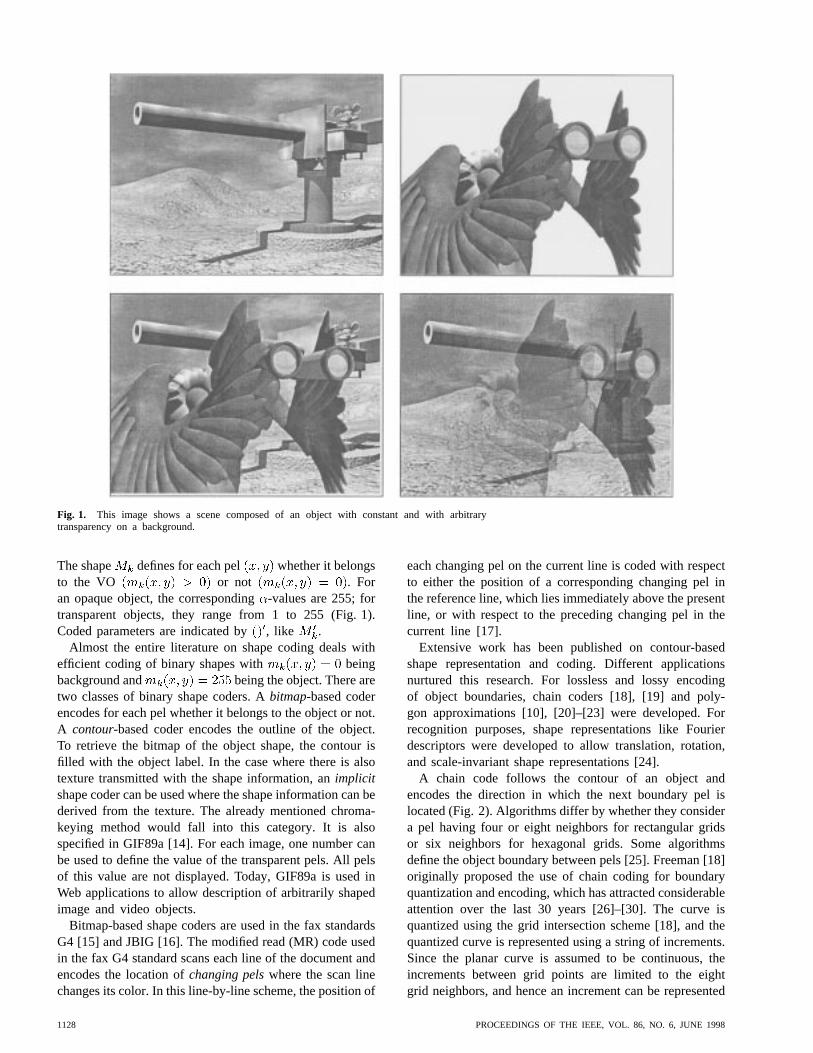
Fig. 1. This image shows a scene composed of an object with constant and with arbitrarytransparency on a background.
The shape defines for each pel whether it belongsto the VO or not . Foran opaque object, the corresponding-values are 255; fortransparent objects, they range from 1 to 255 (Fig. 1).Coded parameters are indicated by, like .
Almost the entire literature on shape coding deals withefficient coding of binary shapes with beingbackground and being the object. There aretwo classes of binary shape coders. Abitmap-based coderencodes for each pel whether it belongs to the object or not.A contour-based coder encodes the outline of the object.To retrieve the bitmap of the object shape, the contour isfilled with the object label. In the case where there is alsotexture transmitted with the shape information, animplicitshape coder can be used where the shape information can bederived from the texture. The already mentioned chroma-keying method would fall into this category. It is alsospecified in GIF89a [14]. For each image, one number canbe used to define the value of the transparent pels. All pelsof this value are not displayed. Today, GIF89a is used inWeb applications to allow description of arbitrarily shapedimage and video objects.
Bitmap-based shape coders are used in the fax standardsG4 [15] and JBIG [16]. The modified read (MR) code usedin the fax G4 standard scans each line of the document andencodes the location ofchanging pelswhere the scan linechanges its color. In this line-by-line scheme, the position of
each changing pel on the current line is coded with respectto either the position of a corresponding changing pel inthe reference line, which lies immediately above the presentline, or with respect to the preceding changing pel in thecurrent line [17].
Extensive work has been published on contour-basedshape representation and coding. Different applicationsnurtured this research. For lossless and lossy encodingof object boundaries, chain coders [18], [19] and poly-gon approximations [10], [20]–[23] were developed. Forrecognition purposes, shape representations like Fourierdescriptors were developed to allow translation, rotation,and scale-invariant shape representations [24].
A chain code follows the contour of an object andencodes the direction in which the next boundary pel islocated (Fig. 2). Algorithms differ by whether they considera pel having four or eight neighbors for rectangular gridsor six neighbors for hexagonal grids. Some algorithmsdefine the object boundary between pels [25]. Freeman [18]originally proposed the use of chain coding for boundaryquantization and encoding, which has attracted considerableattention over the last 30 years [26]–[30]. The curve isquantized using the grid intersection scheme [18], and thequantized curve is represented using a string of increments.Since the planar curve is assumed to be continuous, theincrements between grid points are limited to the eightgrid neighbors, and hence an increment can be represented
1128 PROCEEDINGS OF THE IEEE, VOL. 86, NO. 6, JUNE 1998

Fig. 2. A chain code follows the contour of an object by describing the direction from one boundarypel to the next. Each arrow is represented by one out of four or one out of eight symbols, respectively.On the right, the symbols for differentially encoding the shape are given.
by 3 bits. For lossless encoding of boundary shapes, anaverage 1.2 bits/boundary pels and 1.4 bits/boundary pelsare required, respectively, for a four- and an eight-neighborgrid [19]. There have been many extensions to this basicscheme, such as the generalized chain codes [26], wherethe coding efficiency has been improved by using links ofdifferent length and different angular resolution. In [29],a scheme is presented that utilizes patterns in a chaincode string to increase the coding efficiency. In [30],differential chain codes are presented, which employ thestatistical dependency between successive links. There hasalso been interest in the theoretical performance of chaincodes. In [27], the performance of different quantizationschemes is compared, whereas in [28], the rate-distortioncharacteristics of certain chain codes are studied. In thispaper, we are not concerned with the quantization ofthe continuous curve since we assume that the objectboundaries are given with pixel accuracy. Some chaincodes also include simplifications of the contour in orderto increase coding efficiency [31], [32]. This is similar tofiltering the object shape with morphological filters and thencoding with a chain code. The entropy coder may code acombination of several directions with just one code word.
A polygon-based shape representation was developed forOBASC [8], [20]. As a quality measure, the Euclideandistance between the original and the approximatedcontour is used. During subjective evaluations of commonintermediate format (CIF) (352288 pels) video sequences,it was found that allowing a peak distance ofpel is sufficient to allow proper representations of objectsin low-bit-rate applications. Hence, the lossy polygon ap-proximation was developed. The polygon approximationis computed by using those two contour points with themaximum distance between them as the starting point.Then, additional points are added to the polygon where theapproximation error between the polygon and the contourare maximum (Fig. 3). This is repeated until the shapeapproximation error is less than . In a last step,splines are defined using the polygon points. If the splineapproximation does not result in a larger approximation
error between two neighboring polygon points, the splineapproximation is used. This leads to a smoother representa-tion of the shape (Fig. 4). Vertex coordinates and the curvetype between two vertices are arithmetically encoded.
This polygon/spline representation is also used for codingshapes in intermode. For temporal prediction, the texturemotion vectors are applied to the vertices defining thepredicted shape. Then, all vertices within the allowableapproximation error define the new polygon ap-proximation. It is refined as described above such thatthe entire polygon is within the allowable error . Ina final step, it is again decided whether a polygon orspline approximation is used. The reason for not usinga complete spline approximation is due to the fact thattemporal prediction using splines is less efficient becausethe refinement of a predicted spline representation requiresthe definition of many more new vertices when comparedto a polygon representation.
In [33], B-spline curves are used to approximate aboundary. An optimization procedure is formulated forfinding the optimal locations of the control points byminimizing the mean squared error between the boundaryand the approximation. This is an appropriate objectivewhen the smoothing of the boundary is the main problem.When the resulting control points need to be encoded,however, the tradeoff between the encoding cost and theresulting distortion needs to be considered. By selecting themean squared error as the distortion measure and allowingfor the location of the control points to be anywhere on theplane, the resulting optimization problem is continuous andconvex and can be solved easily. To encode the positionsof the resulting control points efficiently, however, oneneeds to quantize them, and therefore the optimality of thesolution is lost. It is well known that the optimal solution toa discrete optimization problem (quantized locations) doesnot have to be close to the solution of the correspondingcontinuous problem.
The above methods for polygon/spline representationachieve good results but they do not claim optimality.In Section IV, we describe polygon/spline representation
KATSAGGELOS et al.: SHAPE-CODING TECHNIQUES 1129
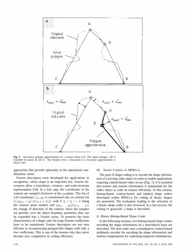
Fig. 3. Successive polygon approximation of a contour (from [7]). The initial polygonAB isextended by pointsB and C. The iteration from a four-point to a five-point approximation isshown here.
approaches that provide optimality in the operational rate-distortion sense.
Fourier descriptors were developed for applications inrecognition, where shape is an important key. Fourier de-scriptors allow a translation-, rotation-, and scale-invariantrepresentation [34]. In a first step, the coordinates of thecontour are sampled clockwise in the-plane. This list of2-D coordinates is transformed into an ordered list
, with beingthe contour point number andthe change of direction of the contour. Since the samplesare periodic over the object boundary perimeter, they canbe expanded into a Fourier series. To preserve the maincharacteristics of a shape, only the large Fourier coefficientshave to be maintained. Fourier descriptors are not veryefficient in reconstructing polygon-like shapes with only afew coefficients. This is one of the reasons why they neverbecame very competitive in coding efficiency.
III. SHAPE CODING IN MPEG-4
The goal of shape coding is to encode the shape informa-tion of a moving video object in order to enable applicationsrequiring content-based video access (Fig. 1). It is assumedthat texture and motion information is transmitted for thevideo object to code its texture efficiently. In this section,bitmap-based, contour-based, and implicit shape codersdeveloped within MPEG-4 for coding of binary shapesare presented. The evaluation leading to the selection ofa binary shape coder is also reviewed. In a last section, thecoding of grayscale -maps is described.
A. Binary Bitmap-Based Shape Coder
In the following sections, two bitmap-based shape codersencoding the shape information on a macroblock basis aredescribed. The first coder uses a nonadaptive context-basedarithmetic encoder for encoding the shape information andmotion compensation for exploiting temporal redundancies.
1130 PROCEEDINGS OF THE IEEE, VOL. 86, NO. 6, JUNE 1998

Fig. 4. Approximation using a polygon/spline approximation (from [64]).
(a) (b)
Fig. 5. Templates for defining the context of the pel to be coded(o). (a) The intramode context. (b) The intermode context. Thealignment is done after motion compensating the previous frameof the video object.
The second coder is based on an adaptation of the MR coderthat is used in place of the arithmetic encoder. Other aspectsof the algorithms are identical.
1) Context-Based (CAE) Shape Coder:Within a mac-roblock, this coder exploits the spatial redundancy of thebinary shape information to be coded. Pels are codedin scan-line order and row by row. In the followingparagraphs, shape encoding in intramode is described [35].Then, this technique is extended to include an intermode[35], [36].
a) Intramode: In intramode, three different types ofmacroblocks are distinguished. Transparent and opaqueblocks are signaled as macroblock type. The macroblockson the object boundary containing transparent as well asopaque pels belong to the third type. For these boundarymacroblocks, a template of 10 pels is used to define thecausal context for predicting the shape value of the currentpel [Fig. 5(a)]. For encoding the state transition, a context-based arithmetic encoder is used. The probability table ofthe arithmetic encoder for the 1024 contexts was derivedfrom sequences that are outside of the test set used forcomparing different shape coders. With two bytes allocatedto describe the symbol probability for each context, thetable size is 2048 bytes. To avoid emulation of start codes,the arithmetic coder stuffs one “1” into the bitstreamwhenever a long sequence of “0”’s is sent.
The template extends up to 2 pels to the left, to theright, and to the top of the pel to be coded [Fig. 5(a)].Hence, for encoding the pels in the two top and left rowsof a macroblock, parts of the template are defined by theshape information of the already transmitted macroblockson the top and on the left side of the current macroblock.For the two right-most columns, each undefined pel of thecontext is set to the value of its closest neighbor inside themacroblock.
To increase coding efficiency as well as to allow lossyshape coding, a macroblock can be subsampled by a factorof two or four, resulting in a subblock of size 88 or4 4 pels, respectively. The subblock is encoded usingthe encoder as described above. The encoder transmits tothe decoder the subsampling factor such that the decoderdecodes the shape data and then upsamples the decodedsubblock to macroblock size. Obviously, encoding theshape using a high subsampling factor is more efficientbut the decoded shape after upsampling may or may notbe the same as the original shape. Hence, this subsamplingis mostly used for lossy shape coding and for rate-controlpurposes.
Depending on the upsampling filter, the decoded shapecan look somewhat blocky. Several upsampling filters wereinvestigated. The two best performing filters were a simplepel replication filter combined with a 33 median filter andan adaptive nonlinear upsampling filter. The context of thisupsampling filter as standardized by MPEG-4 is shown inFig. 6.
The efficiency of the shape coder differs depending onthe orientation of the shape data. Therefore, the encoder canchoose to code the block as described above or transposethe macroblock prior to arithmetic coding.
b) Intermode: To exploit temporal redundancy in theshape information, the coder described above is extended byan intermode requiring motion compensation and a differenttemplate for defining the context.
KATSAGGELOS et al.: SHAPE-CODING TECHNIQUES 1131

Fig. 6. The upsampled pels(x) lie between the location of thesubsampled pels(o). Neighboring pels (boldo) defining the valuesof the pels to be upsampled (boldx).
For motion compensation, a 2-D integer pel motionvector is estimated using full search for each macroblockin order to minimize the prediction error between the pre-viously coded shape and the current shape . Theshape motion vectors are predictively encoded with respectto the shape motion vectors of neighboring macroblocks. Ifno shape motion vector is available for prediction, texturemotion vectors are used as predictors. The shape motionvector of the current block is used to align a new templatedesigned for coding shape in intermode [Fig. 5(b)]. Thetemplate defines a context of 9 pels, resulting in 512contexts. The probability for one symbol is described by2 bytes, giving a probability table size of 1024 bytes. Fourpels of the context are neighbors of the pel to be coded; 5pels are located at the motion-compensated location in theprevious frame. Assuming that the motion vectorpoints from the current to the previous coded ,the part of the template located in the previously codedshape is centered at , with beingthe location of the current pel to be coded.
In intermode, the same options as in intramode, likesubsampling and transposing, are available. For lossy shapecoding, the encoder may also decide that the shape rep-resentation achieved by just carrying out motion com-pensation is sufficient, thus saving bits by avoiding thecoding of the prediction error. The encoder can selectone of seven modes for the shape information of eachmacroblock: transparent, opaque, intra, inter with/withoutshape motion vectors, and inter with/without shape motionvectors and prediction error coding. These different optionswith optional subsampling and transposition allow for en-coder implementations of different coding efficiency andimplementation complexity.
2) Modified MR (MMR) Shape Coder:The MMR shapecoder is a macroblock-based shape coder [36]. In com-parison to the CAE shape coder, the MMR shape codermainly replaces the context-based arithmetic encoder andthe templates by a MMR coder. Therefore, the descriptionof the MMR shape coder is limited to the MMR coder. ThisMMR coder is derived from the modified read coder in thefax G4 standard [15].
Fig. 7 is used for describing the encoding procedure. Forsimplicity, it is assumed that the macroblock to be codedis subsampled by a factor of two, resulting in a subblockof size 8 8 pels to be coded. Each block is coded in raster-scan order. Within each line, the position of pels on theobject boundary is encoded. In Fig. 7, it is assumed that
(a) (b)
Fig. 7. Changing pels are used in modified MMR shape codingto define object boundaries.
the top five rows of the block have already been coded;hence, the coder knows the position of the pelsand
in the current block as well as pels and in themotion-compensated block when coding in intramode andintermode, respectively.
a) Intramode: The unknown point on the objectboundary is encoded with reference to the two pels,and . is the last changing pel encoded prior to.is the first changing pel on the line above, to the right of
, and with the opposite color of , if such a point exists(Fig. 7). If not, then is the left-most changing pel on thesame line as . To encode the distance between and
, one of the three modes—vertical, horizontal, or verticalpass—is selected. Assuming that all pels are numbered inraster-scan order starting with zero in the top-left cornerof the block, i.e., in Fig. 7 , and columnsare numbered from left to right, i.e., , a mode isselected according to
modeVertical ifHorizontal if widthVertical Pass otherwise
(2)
with the threshold for no subsampling, for asubsampling factor of two, for a subsampling factorof four, andwidth is the width of the block to be coded.
In vertical mode, the distance is encodedusing one of eight variable-length coder (VLC) tables thatis selected according to the object boundary direction, asdefined by a template positioned above pel(Fig. 8).
In horizontal mode, the position of is encoded as itsdistance to . Just due to the fact that the horizontal andnot the vertical mode is selected, the decoder can sometimesdeduct the minimum distance between and . In thiscase, only the difference with respect to this minimumdistance is encoded.
In vertical pass mode, one code word is sent for each linewithout an object boundary. One last code word codes theremaining distance to the next point on the object boundary.
in Fig. 7 (subsampling factor of two) is encoded usingvertical pass mode.
The efficiency of the shape coder differs depending onthe orientation of the shape data. Therefore, the encoder can
1132 PROCEEDINGS OF THE IEEE, VOL. 86, NO. 6, JUNE 1998
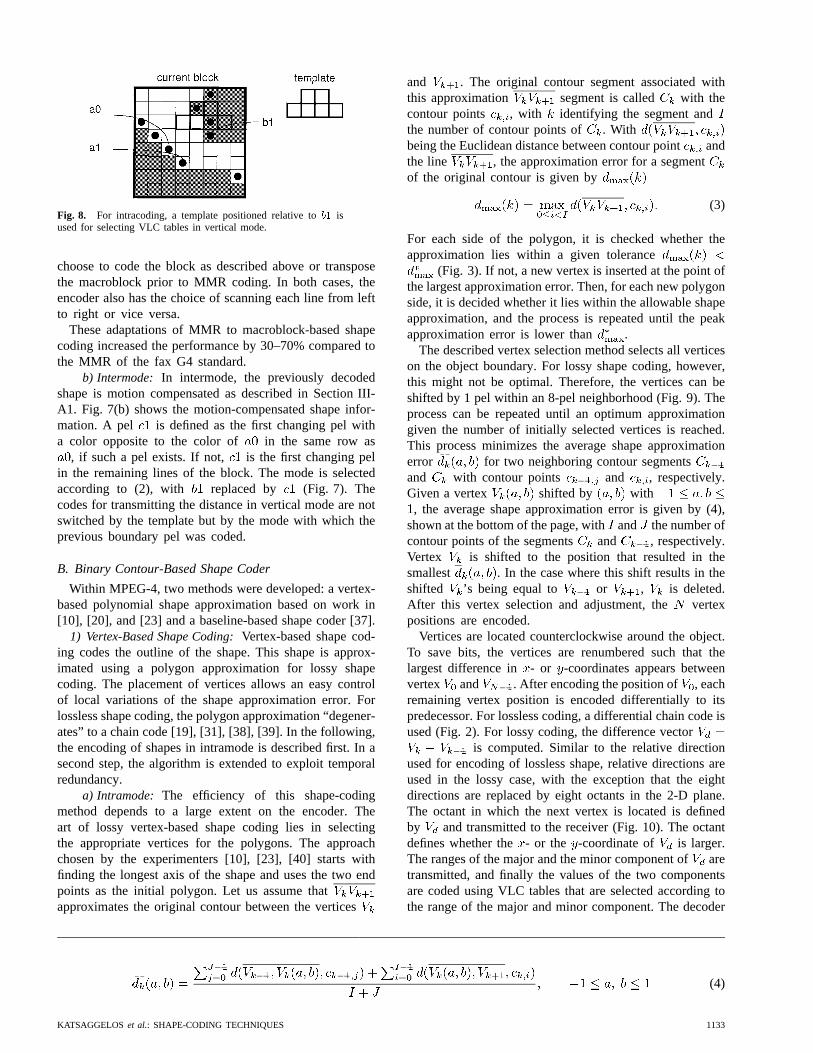
Fig. 8. For intracoding, a template positioned relative tob1 isused for selecting VLC tables in vertical mode.
choose to code the block as described above or transposethe macroblock prior to MMR coding. In both cases, theencoder also has the choice of scanning each line from leftto right or vice versa.
These adaptations of MMR to macroblock-based shapecoding increased the performance by 30–70% compared tothe MMR of the fax G4 standard.
b) Intermode: In intermode, the previously decodedshape is motion compensated as described in Section III-A1. Fig. 7(b) shows the motion-compensated shape infor-mation. A pel is defined as the first changing pel witha color opposite to the color of in the same row as
, if such a pel exists. If not, is the first changing pelin the remaining lines of the block. The mode is selectedaccording to (2), with replaced by (Fig. 7). Thecodes for transmitting the distance in vertical mode are notswitched by the template but by the mode with which theprevious boundary pel was coded.
B. Binary Contour-Based Shape Coder
Within MPEG-4, two methods were developed: a vertex-based polynomial shape approximation based on work in[10], [20], and [23] and a baseline-based shape coder [37].
1) Vertex-Based Shape Coding:Vertex-based shape cod-ing codes the outline of the shape. This shape is approx-imated using a polygon approximation for lossy shapecoding. The placement of vertices allows an easy controlof local variations of the shape approximation error. Forlossless shape coding, the polygon approximation “degener-ates” to a chain code [19], [31], [38], [39]. In the following,the encoding of shapes in intramode is described first. In asecond step, the algorithm is extended to exploit temporalredundancy.
a) Intramode: The efficiency of this shape-codingmethod depends to a large extent on the encoder. Theart of lossy vertex-based shape coding lies in selectingthe appropriate vertices for the polygons. The approachchosen by the experimenters [10], [23], [40] starts withfinding the longest axis of the shape and uses the two endpoints as the initial polygon. Let us assume thatapproximates the original contour between the vertices
and . The original contour segment associated withthis approximation segment is called with thecontour points , with identifying the segment andthe number of contour points of . Withbeing the Euclidean distance between contour pointandthe line , the approximation error for a segmentof the original contour is given by
(3)
For each side of the polygon, it is checked whether theapproximation lies within a given tolerance
(Fig. 3). If not, a new vertex is inserted at the point ofthe largest approximation error. Then, for each new polygonside, it is decided whether it lies within the allowable shapeapproximation, and the process is repeated until the peakapproximation error is lower than .
The described vertex selection method selects all verticeson the object boundary. For lossy shape coding, however,this might not be optimal. Therefore, the vertices can beshifted by 1 pel within an 8-pel neighborhood (Fig. 9). Theprocess can be repeated until an optimum approximationgiven the number of initially selected vertices is reached.This process minimizes the average shape approximationerror for two neighboring contour segmentsand with contour points and , respectively.Given a vertex shifted by with
, the average shape approximation error is given by (4),shown at the bottom of the page, withand the number ofcontour points of the segments and , respectively.Vertex is shifted to the position that resulted in thesmallest . In the case where this shift results in theshifted ’s being equal to or , is deleted.After this vertex selection and adjustment, the vertexpositions are encoded.
Vertices are located counterclockwise around the object.To save bits, the vertices are renumbered such that thelargest difference in - or -coordinates appears betweenvertex and . After encoding the position of , eachremaining vertex position is encoded differentially to itspredecessor. For lossless coding, a differential chain code isused (Fig. 2). For lossy coding, the difference vector
is computed. Similar to the relative directionused for encoding of lossless shape, relative directions areused in the lossy case, with the exception that the eightdirections are replaced by eight octants in the 2-D plane.The octant in which the next vertex is located is definedby and transmitted to the receiver (Fig. 10). The octantdefines whether the- or the -coordinate of is larger.The ranges of the major and the minor component ofaretransmitted, and finally the values of the two componentsare coded using VLC tables that are selected according tothe range of the major and minor component. The decoder
(4)
KATSAGGELOS et al.: SHAPE-CODING TECHNIQUES 1133
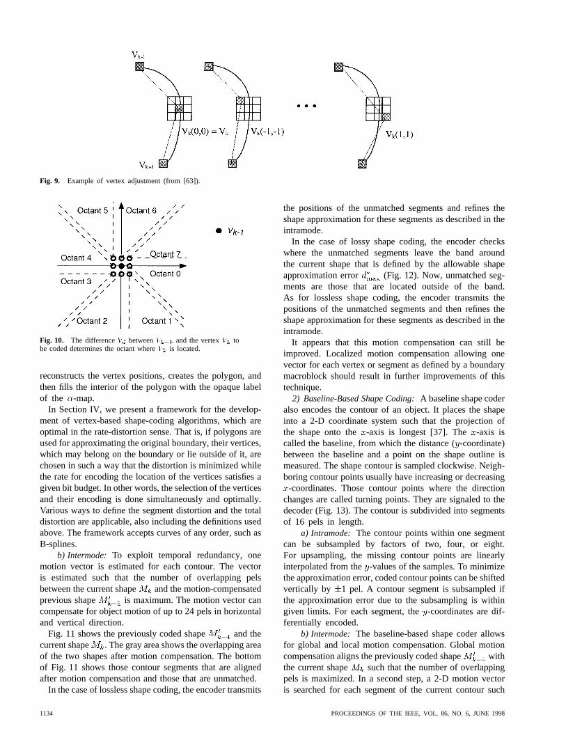
Fig. 9. Example of vertex adjustment (from [63]).
Fig. 10. The differenceVd betweenVk�1 and the vertexVk tobe coded determines the octant whereVk is located.
reconstructs the vertex positions, creates the polygon, andthen fills the interior of the polygon with the opaque labelof the -map.
In Section IV, we present a framework for the develop-ment of vertex-based shape-coding algorithms, which areoptimal in the rate-distortion sense. That is, if polygons areused for approximating the original boundary, their vertices,which may belong on the boundary or lie outside of it, arechosen in such a way that the distortion is minimized whilethe rate for encoding the location of the vertices satisfies agiven bit budget. In other words, the selection of the verticesand their encoding is done simultaneously and optimally.Various ways to define the segment distortion and the totaldistortion are applicable, also including the definitions usedabove. The framework accepts curves of any order, such asB-splines.
b) Intermode: To exploit temporal redundancy, onemotion vector is estimated for each contour. The vectoris estimated such that the number of overlapping pelsbetween the current shape and the motion-compensatedprevious shape is maximum. The motion vector cancompensate for object motion of up to 24 pels in horizontaland vertical direction.
Fig. 11 shows the previously coded shape and thecurrent shape . The gray area shows the overlapping areaof the two shapes after motion compensation. The bottomof Fig. 11 shows those contour segments that are alignedafter motion compensation and those that are unmatched.
In the case of lossless shape coding, the encoder transmits
the positions of the unmatched segments and refines theshape approximation for these segments as described in theintramode.
In the case of lossy shape coding, the encoder checkswhere the unmatched segments leave the band aroundthe current shape that is defined by the allowable shapeapproximation error (Fig. 12). Now, unmatched seg-ments are those that are located outside of the band.As for lossless shape coding, the encoder transmits thepositions of the unmatched segments and then refines theshape approximation for these segments as described in theintramode.
It appears that this motion compensation can still beimproved. Localized motion compensation allowing onevector for each vertex or segment as defined by a boundarymacroblock should result in further improvements of thistechnique.
2) Baseline-Based Shape Coding:A baseline shape coderalso encodes the contour of an object. It places the shapeinto a 2-D coordinate system such that the projection ofthe shape onto the-axis is longest [37]. The -axis iscalled the baseline, from which the distance (-coordinate)between the baseline and a point on the shape outline ismeasured. The shape contour is sampled clockwise. Neigh-boring contour points usually have increasing or decreasing
-coordinates. Those contour points where the directionchanges are called turning points. They are signaled to thedecoder (Fig. 13). The contour is subdivided into segmentsof 16 pels in length.
a) Intramode: The contour points within one segmentcan be subsampled by factors of two, four, or eight.For upsampling, the missing contour points are linearlyinterpolated from the -values of the samples. To minimizethe approximation error, coded contour points can be shiftedvertically by 1 pel. A contour segment is subsampled ifthe approximation error due to the subsampling is withingiven limits. For each segment, the-coordinates are dif-ferentially encoded.
b) Intermode: The baseline-based shape coder allowsfor global and local motion compensation. Global motioncompensation aligns the previously coded shape withthe current shape such that the number of overlappingpels is maximized. In a second step, a 2-D motion vectoris searched for each segment of the current contour such
1134 PROCEEDINGS OF THE IEEE, VOL. 86, NO. 6, JUNE 1998
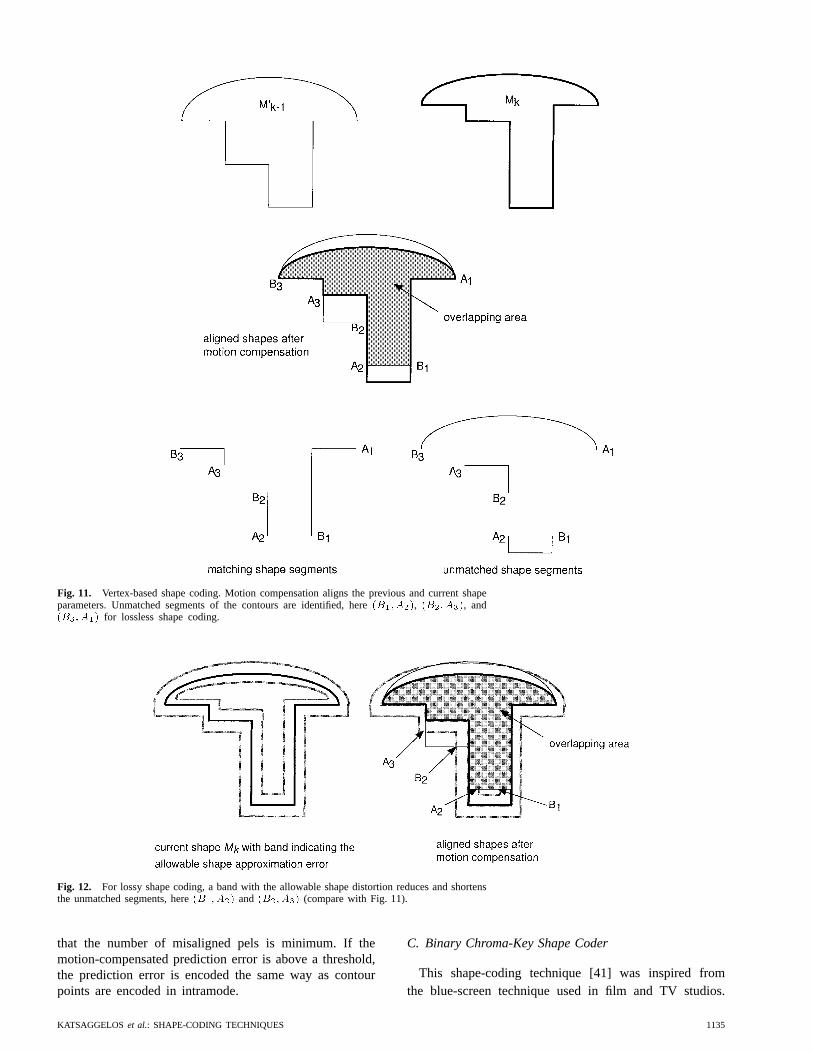
Fig. 11. Vertex-based shape coding. Motion compensation aligns the previous and current shapeparameters. Unmatched segments of the contours are identified, here(B1; A2), (B2; A3), and(B3; A1) for lossless shape coding.
Fig. 12. For lossy shape coding, a band with the allowable shape distortion reduces and shortensthe unmatched segments, here(B1; A2) and (B2; A3) (compare with Fig. 11).
that the number of misaligned pels is minimum. If themotion-compensated prediction error is above a threshold,the prediction error is encoded the same way as contourpoints are encoded in intramode.
C. Binary Chroma-Key Shape Coder
This shape-coding technique [41] was inspired fromthe blue-screen technique used in film and TV studios.
KATSAGGELOS et al.: SHAPE-CODING TECHNIQUES 1135
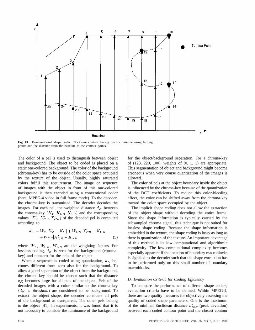
Fig. 13. Baseline-based shape coder. Clockwise contour tracing from a baseline using turningpoints and the distance from the baseline to the contour points.
The color of a pel is used to distinguish between objectand background. The object to be coded is placed on astatic one-colored background. The color of the background(chroma-key) has to be outside of the color space occupiedby the texture of the object. Usually, highly saturatedcolors fulfill this requirement. The image or sequenceof images with the object in front of this one-coloredbackground is then encoded using a conventional coder(here, MPEG-4 video in full frame mode). To the decoder,the chroma-key is transmitted. The decoder decodes theimages. For each pel, the weighted distance betweenthe chroma-key and the correspondingvalues of the decoded pel is computedaccording to
(5)
where , , are the weighting factors. Forlossless coding, is zero for the background (chroma-key) and nonzero for the pels of the object.
When a sequence is coded using quantization,be-comes different from zero also for the background. Toallow a good separation of the object from the background,the chroma-key should be chosen such that the distance
becomes large for all pels of the object. Pels of thedecoded images with a color similar to the chroma-key
threshold are considered to be background. Toextract the object shape, the decoder considers all pelsof the background as transparent. The other pels belongto the object [41]. In experiments, it was found that it isnot necessary to consider the luminance of the background
for the object/background separation. For a chroma-keyof (128, 220, 100), weights of (0, 1, 1) are appropriate.This segmentation of object and background might becomeerroneous when very coarse quantization of the images isallowed.
The color of pels at the object boundary inside the objectis influenced by the chroma-key because of the quantizationof the DCT coefficients. To reduce this color-bleedingeffect, the color can be shifted away from the chroma-keytoward the color space occupied by the object.
The implicit shape coding does not allow the extractionof the object shape without decoding the entire frame.Since the shape information is typically carried by thesubsampled chroma signal, this technique is not suited forlossless shape coding. Because the shape information isembedded in the texture, the shape coding is lossy as long asthere is quantization of the texture. An important advantageof this method is its low computational and algorithmiccomplexity. The low computational complexity becomesespecially apparent if the location of boundary macroblocksis signaled to the decoder such that the shape extraction hasto be performed only on this small number of boundarymacroblocks.
D. Evaluation Criteria for Coding Efficiency
To compare the performance of different shape coders,evaluation criteria have to be defined. Within MPEG-4,there are two quality measures for objectively assessing thequality of coded shape parameters. One is the maximumof the minimal Euclidean distance (peak deviation)between each coded contour point and the closest contour
1136 PROCEEDINGS OF THE IEEE, VOL. 86, NO. 6, JUNE 1998
(a) (b) (c)
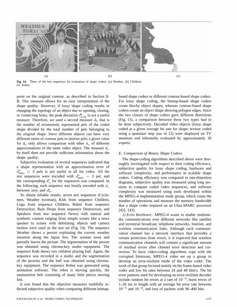
Fig. 14. Three of the test sequences for evaluation of shape coders. (a) Weather. (b) Children.(c) Robot.
point on the original contour, as described in Section II-B. This measure allows for an easy interpretation of theshape quality. However, if lossy shape coding results inchanging the topology of an object due to opening, closing,or connecting holes, the peak deviation is not a usefulmeasure. Therefore, we used a second measurethat isthe number of erroneously represented pels of the codedshape divided by the total number of pels belonging tothe original shape. Since different objects can have verydifferent ratios of contour pels to interior pels, a given valuefor only allows comparison with other of differentapproximations of the same video object. The measureby itself does not provide sufficient information about theshape quality.
Subjective evaluation of several sequences indicated thata shape representation with an approximation error of
pels is not useful at all for video. All thetest sequences were encoded with pel, andthe corresponding for the sequences was computed. Inthe following, each sequence was lossily encoded withbetween zero and .
To obtain reliable results, seven test sequences (Cycla-men, Weather (woman), Kids from sequence Children,Logo from sequence Children, Robot from sequenceDestruction, Rain Drops from sequence Destruction, andSpeakers from test sequence News) with natural andsynthetic content ranging from simple scenes like a newsspeaker to scenes with deforming objects and cameramotion were used as the test set (Fig. 14). The sequenceWeather shows a person explaining the current weathersituation along the Japan Sea. The woman turns andpartially leaves the picture. The segmentation of the personwas obtained using chroma-key studio equipment. Thesequence Kids shows two children playing ball. Again, thesequence was recorded in a studio and the segmentationof the persons and the ball was obtained using chroma-key equipment. The sequence Robot was generated usinganimation software. The robot is moving quickly, theammunition belt consisting of many little pieces movingfast.
It was found that the objective measures truthfully re-flected subjective quality when comparing different bitmap-
based shape coders or different contour-based shape coders.For lossy shape coding, the bitmap-based shape coderscreate blocky object shapes, whereas contour-based shapecoders create an object shape showing polygon edges. Sincethe two classes of shape coders gave different distortions(Fig. 15), a comparison between these two types had tobe done subjectively. Decoded video objects (lossy shapecoded at a given average bit rate for shape; texture codedusing a quantizer step size of 12) were displayed on TVmonitors and informally evaluated by approximately 30experts.
E. Comparison of Binary Shape Coders
The shape-coding algorithms described above were thor-oughly investigated with respect to their coding efficiency,subjective quality for lossy shape coding, hardware andsoftware complexity, and performance in scalable shapecoders. Coding efficiency was compared in rate-distortiondiagrams, subjective quality was measured using long ses-sions to compare coded video sequences, and softwarecomplexity was measured using tools developed withinthe MPEG-4 implementation study group, which count thenumber of operations and measure the memory bandwidththat a shape coder required on an Ultra-SPARC processor[42], [43].
1) Error Resilience: MPEG-4 wants to enable multime-dia communications over different networks like satelliteand terrestrial broadcast, telephone networks, Internet, andwireless communication links. Although each communi-cation channel has a network interface that provides acertain protection from errors, it is expected that wirelesscommunication channels will contain a significant amountof residual errors after channel error detection and cor-rection. To have video-coding algorithms cope with thecorrupted bitstream, MPEG-4 video set up a group todevelop an error-resilient mode of the video coder. Thework of that group focused mainly on the frame-based videocoder and low bit rates between 24 and 48 kbit/s. The biterror patterns used for developing an error-resilient decoderinclude random bit errors at a rate of 10, burst errors of1–20 ms in length with an average bit error rate between10 and 10 , and loss of packets with 96–400 bits.
KATSAGGELOS et al.: SHAPE-CODING TECHNIQUES 1137
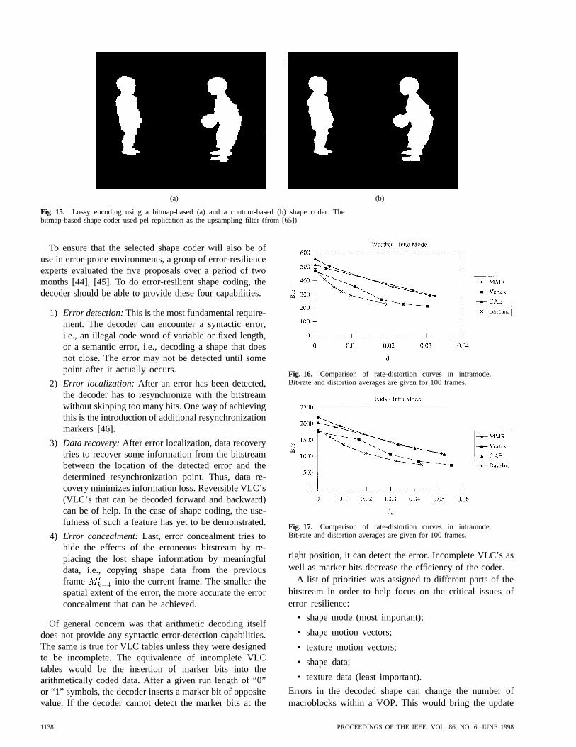
(a) (b)
Fig. 15. Lossy encoding using a bitmap-based (a) and a contour-based (b) shape coder. Thebitmap-based shape coder used pel replication as the upsampling filter (from [65]).
To ensure that the selected shape coder will also be ofuse in error-prone environments, a group of error-resilienceexperts evaluated the five proposals over a period of twomonths [44], [45]. To do error-resilient shape coding, thedecoder should be able to provide these four capabilities.
1) Error detection:This is the most fundamental require-ment. The decoder can encounter a syntactic error,i.e., an illegal code word of variable or fixed length,or a semantic error, i.e., decoding a shape that doesnot close. The error may not be detected until somepoint after it actually occurs.
2) Error localization: After an error has been detected,the decoder has to resynchronize with the bitstreamwithout skipping too many bits. One way of achievingthis is the introduction of additional resynchronizationmarkers [46].
3) Data recovery:After error localization, data recoverytries to recover some information from the bitstreambetween the location of the detected error and thedetermined resynchronization point. Thus, data re-covery minimizes information loss. Reversible VLC’s(VLC’s that can be decoded forward and backward)can be of help. In the case of shape coding, the use-fulness of such a feature has yet to be demonstrated.
4) Error concealment:Last, error concealment tries tohide the effects of the erroneous bitstream by re-placing the lost shape information by meaningfuldata, i.e., copying shape data from the previousframe into the current frame. The smaller thespatial extent of the error, the more accurate the errorconcealment that can be achieved.
Of general concern was that arithmetic decoding itselfdoes not provide any syntactic error-detection capabilities.The same is true for VLC tables unless they were designedto be incomplete. The equivalence of incomplete VLCtables would be the insertion of marker bits into thearithmetically coded data. After a given run length of “0”or “1” symbols, the decoder inserts a marker bit of oppositevalue. If the decoder cannot detect the marker bits at the
Fig. 16. Comparison of rate-distortion curves in intramode.Bit-rate and distortion averages are given for 100 frames.
Fig. 17. Comparison of rate-distortion curves in intramode.Bit-rate and distortion averages are given for 100 frames.
right position, it can detect the error. Incomplete VLC’s aswell as marker bits decrease the efficiency of the coder.
A list of priorities was assigned to different parts of thebitstream in order to help focus on the critical issues oferror resilience:
• shape mode (most important);
• shape motion vectors;
• texture motion vectors;
• shape data;
• texture data (least important).
Errors in the decoded shape can change the number ofmacroblocks within a VOP. This would bring the update
1138 PROCEEDINGS OF THE IEEE, VOL. 86, NO. 6, JUNE 1998
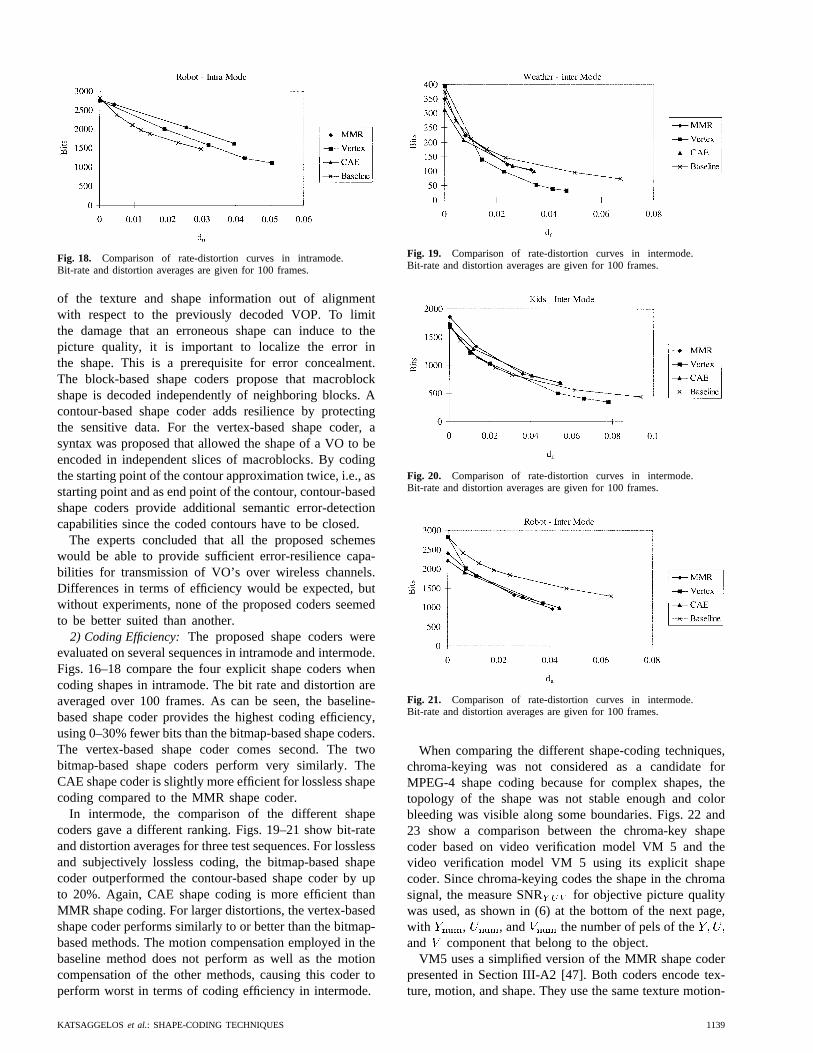
Fig. 18. Comparison of rate-distortion curves in intramode.Bit-rate and distortion averages are given for 100 frames.
of the texture and shape information out of alignmentwith respect to the previously decoded VOP. To limitthe damage that an erroneous shape can induce to thepicture quality, it is important to localize the error inthe shape. This is a prerequisite for error concealment.The block-based shape coders propose that macroblockshape is decoded independently of neighboring blocks. Acontour-based shape coder adds resilience by protectingthe sensitive data. For the vertex-based shape coder, asyntax was proposed that allowed the shape of a VO to beencoded in independent slices of macroblocks. By codingthe starting point of the contour approximation twice, i.e., asstarting point and as end point of the contour, contour-basedshape coders provide additional semantic error-detectioncapabilities since the coded contours have to be closed.
The experts concluded that all the proposed schemeswould be able to provide sufficient error-resilience capa-bilities for transmission of VO’s over wireless channels.Differences in terms of efficiency would be expected, butwithout experiments, none of the proposed coders seemedto be better suited than another.
2) Coding Efficiency:The proposed shape coders wereevaluated on several sequences in intramode and intermode.Figs. 16–18 compare the four explicit shape coders whencoding shapes in intramode. The bit rate and distortion areaveraged over 100 frames. As can be seen, the baseline-based shape coder provides the highest coding efficiency,using 0–30% fewer bits than the bitmap-based shape coders.The vertex-based shape coder comes second. The twobitmap-based shape coders perform very similarly. TheCAE shape coder is slightly more efficient for lossless shapecoding compared to the MMR shape coder.
In intermode, the comparison of the different shapecoders gave a different ranking. Figs. 19–21 show bit-rateand distortion averages for three test sequences. For losslessand subjectively lossless coding, the bitmap-based shapecoder outperformed the contour-based shape coder by upto 20%. Again, CAE shape coding is more efficient thanMMR shape coding. For larger distortions, the vertex-basedshape coder performs similarly to or better than the bitmap-based methods. The motion compensation employed in thebaseline method does not perform as well as the motioncompensation of the other methods, causing this coder toperform worst in terms of coding efficiency in intermode.
Fig. 19. Comparison of rate-distortion curves in intermode.Bit-rate and distortion averages are given for 100 frames.
Fig. 20. Comparison of rate-distortion curves in intermode.Bit-rate and distortion averages are given for 100 frames.
Fig. 21. Comparison of rate-distortion curves in intermode.Bit-rate and distortion averages are given for 100 frames.
When comparing the different shape-coding techniques,chroma-keying was not considered as a candidate forMPEG-4 shape coding because for complex shapes, thetopology of the shape was not stable enough and colorbleeding was visible along some boundaries. Figs. 22 and23 show a comparison between the chroma-key shapecoder based on video verification model VM 5 and thevideo verification model VM 5 using its explicit shapecoder. Since chroma-keying codes the shape in the chromasignal, the measure SNR for objective picture qualitywas used, as shown in (6) at the bottom of the next page,with , , and the number of pels of theand component that belong to the object.
VM5 uses a simplified version of the MMR shape coderpresented in Section III-A2 [47]. Both coders encode tex-ture, motion, and shape. They use the same texture motion-
KATSAGGELOS et al.: SHAPE-CODING TECHNIQUES 1139
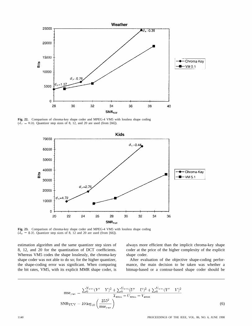
Fig. 22. Comparison of chroma-key shape coder and MPEG-4 VM5 with lossless shape coding(dn = 0:0). Quantizer step sizes of 8, 12, and 20 are used (from [66]).
Fig. 23. Comparison of chroma-key shape coder and MPEG-4 VM5 with lossless shape coding(dn = 0:0). Quantizer step sizes of 8, 12 and 20 are used (from [66]).
estimation algorithm and the same quantizer step sizes of8, 12, and 20 for the quantization of DCT coefficients.Whereas VM5 codes the shape losslessly, the chroma-keyshape coder was not able to do so; for the higher quantizer,the shape-coding error was significant. When comparingthe bit rates, VM5, with its explicit MMR shape coder, is
always more efficient than the implicit chroma-key shapecoder at the price of the higher complexity of the explicitshape coder.
After evaluation of the objective shape-coding perfor-mance, the main decision to be taken was whether abitmap-based or a contour-based shape coder should be
mse
SNRmse
(6)
1140 PROCEEDINGS OF THE IEEE, VOL. 86, NO. 6, JUNE 1998

Table 1 Comparison Between the Block-Based CAE Shape Coder and the Contour-BasedVertex-Based Shape Coder Based on Seven Test Sequences. Relative Statements Are Always withRespect to the Other Shape Coder. Please Note that This Is a Snapshot as of April 1997
selected for the MPEG-4 standard. To ease this decision,the group working on shape coding first selected the bestcontour-based and best block-based shape coders.
As far as bitmap-based shape coding is concerned, theCAE shape coder outperformed the MMR shape coder.For the contour-based shape coding, the vertex-based coderwas chosen. It outperformed the baseline-based coder incoding efficiency for intermode as well as in terms ofcomputational complexity. Furthermore, the baseline coderwas implemented only once, whereas all the other shapecoders had two independent implementations.
3) Hardware Implementation:The Implementation Stud-ies Group of MPEG-4 evaluated the vertex-based andcontext-based shape coders with respect to hardware-implementation implications. It is assumed that most ofthe computations will be done using programmable logiclike video signal processors.
When comparing a VLC decoder as used for the vertex-based methods with the arithmetic decoder used in thecontext-based shape coder, an arithmetic decoder was foundto be more difficult to implement and to require more chipsurface.
However, the real bottleneck of a video decoder willbe the required bandwidth for off-chip memory accessand caching [48]. Here, the block-based, context-basedshape coder has the advantage that the entire shape blockcan be loaded into on-chip cache and processed. At theend of decoding, the decoded block can be written tomemory. Since blocks are processed in predefined order,address generation for memory access is straightforward.The vertex-based shape coder does not allow for predefined
memory access since no prior knowledge is available asto how the polygon will extend from one vertex to thenext. Hence, cache prefetching will not work efficiently,and loading the entire shape image into on-chip cache isnot an option due to the size limitation of the cache. Afurther disadvantage of the vertex-based shape coder is thatthe decoding time depends on the number of vertices andthe shape of the object. This is in contrast to the fixedprocessing time required for context-based shape coding,allowing for easier task scheduling on the processor.
4) Summary:As far as shape-coding requirements areconcerned, all explicit shape coders are able to providelossless, subjectively lossless, and lossy shape coding.The algorithms can be extended to scalable shape coders,bitstream editing, shape-only decoding, and low-delay ap-plications, as well as applications using noisy transmissionchannels. Table 1 compares the context-based and vertex-based shape coders, as done at the Bristol MPEG meetingin April 1997. None of the algorithms clearly outperformsthe other. However, it was felt that the simple hardwareimplementation of the context-based shape coder was areason to reject the vertex-based shape coder. After thatmeeting, the competitive phase of shape coding ended, andMPEG-4 focused on optimizing the selected context-basedshape coder mainly by developing the adaptive upsamplingfilter (Fig. 6) and an error-resilient shape coding mode.
F. Grayscale Shape Coder
Grayscale alpha maps allow 8 bits for each luminancepel to define the transparency of that pel. Transparency isan important tool for composing objects into scenes and
KATSAGGELOS et al.: SHAPE-CODING TECHNIQUES 1141
special effects (Fig. 1). Two types of transparencies aredistinguished: binary alpha maps for objects with constanttransparency and arbitrary alpha maps for objects withvarying transparency.
1) Objects with Constant Transparency:For a transparentobject that does not have a varying transparency, the shapeis encoded using the binary shape coder and the 8-bit valueof the alpha map. To avoid aliasing, grayscale alpha mapsusually have lower transparency values at the boundary.Blending the alpha map near the object boundary can besupported by transmitting the coefficients of a 33 pel finite-duration impulse response filter that is applied to the alphamap within a stripe on the inner object boundary. The stripecan be up to 3 pels wide.
2) Objects with Arbitrary Transparency:For arbitrary al-pha maps, shape coding is done in two steps [49]. In thefirst step, the outline of the object is losslessly encodedas a binary shape. In the second step, the actual alphamap is treated like the luminance of an object with binaryshape and coded using the MPEG-4 texture-coding tools ofpadding, motion compensation, and DCT.
IV. OPTIMAL CONTOUR ENCODING IN
THE RATE-DISTORTION SENSE
A. Introduction
We now present a framework for contour encoding thatis optimal in the rate-distortion sense. We formulate theproblem in various ways. The contour approximation canbe done using a polygon, B-splines, or higher order curves.In all cases, the problem reduces to finding the shortest pathin a directed acyclic graph (DAG).
Before continuing, it is worthwhile to present a review ofB-splines. These are a family of parametric curves that haveproven to be very useful in boundary encoding [50]–[52].In the following discussion, we will concentrate on second-order B-splines. However, this theory can be generalized tohigher order curves. Also, it should be noted that first-orderB-splines are equivalent to polygons.
A B-spline is a specific curve type from the family ofparametric curves [53]. A parametric curve consists of oneor more curve segments. Each curve segment is definedby control points,where defines the degree ofthe curve. The control points are located around the curvesegment, and together with a constant base matrix, thecontrol points solely define the shape of the curve. A 2-Dcurve segment with control points
is defined as follows:
forotherwise.
(7)
The points at the beginning and end of a curve segmentare called knots and can be found by setting and
. The following is the definition for a second-degreecurve segment, with as index for the different curvesegments and and , respectively, as the horizontal
and vertical coordinates of control point :
(8)
Both the base matrix , with specific constant param-eters for each specific type of parametric curve, and thecontrol point matrix , with control points, definethe shape of in a two-dimensional plane. Every pointof the curve segment can be calculated with (8) by letting
vary from zero to one. Every curve segment can becalculated independently in order to calculate the entirecurve , consisting of curve segments, which is ofthe following form:
(9)
Among common parametric curves are the Bezier curve andthe B-spline curve. For the proposed shape-coding methodin this section, we chose a second-order (quadratic) basisuniform nonrational B-spline curve [53] with the followingbase matrix:
(10)
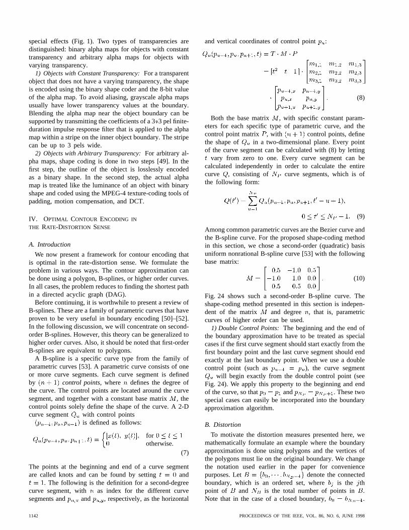
Fig. 24 shows such a second-order B-spline curve. Theshape-coding method presented in this section is indepen-dent of the matrix and degree , that is, parametriccurves of higher order can be used.
1) Double Control Points:The beginning and the end ofthe boundary approximation have to be treated as specialcases if the first curve segment should start exactly from thefirst boundary point and the last curve segment should endexactly at the last boundary point. When we use a doublecontrol point (such as ), the curve segment
will begin exactly from the double control point (seeFig. 24). We apply this property to the beginning and endof the curve, so that and . These twospecial cases can easily be incorporated into the boundaryapproximation algorithm.
B. Distortion
To motivate the distortion measures presented here, wemathematically formulate an example where the boundaryapproximation is done using polygons and the vertices ofthe polygons must lie on the original boundary. We changethe notation used earlier in the paper for conveniencepurposes. Let denote the connectedboundary, which is an ordered set, where is the thpoint of and is the total number of points in .Note that in the case of a closed boundary, .
1142 PROCEEDINGS OF THE IEEE, VOL. 86, NO. 6, JUNE 1998
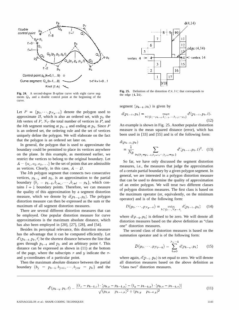
Fig. 24. A second-degree B-spline curve with eight curve seg-mentsQu and a double control point at the beginning of thecurve.
Let denote the polygon used toapproximate , which is also an ordered set, with the
th vertex of , the total number of vertices in , andthe th segment starting at and ending at . Sinceis an ordered set, the ordering rule and the set of verticesuniquely define the polygon. We will elaborate on the factthat the polygon is an ordered set later on.
In general, the polygon that is used to approximate theboundary could be permitted to place its vertices anywhereon the plane. In this example, as mentioned earlier, werestrict the vertices to belong to the original boundary. Let
be the set of points that are admissibleas vertices. Clearly, in this case, .
The th polygon segment that connects two consecutivevertices, and , is an approximation to the partialboundary , which con-tains boundary points. Therefore, we can measurethe quality of this approximation by a segment distortionmeasure, which we denote by . The polygondistortion measure can then be expressed as the sum or themaximum of all segment distortion measures.
There are several different distortion measures that canbe employed. One popular distortion measure for curveapproximations is the maximum absolute distance, whichhas also been employed in [20], [27], [28], and [54].
Besides its perceptual relevance, this distortion measurehas the advantage that it can be computed efficiently. Let
be the shortest distance between the line thatgoes through and and an arbitrary point. Thisdistance can be expressed as shown in (11) at the bottomof the page, where the subscriptsand indicate the -and -coordinates of a particular point.
Then the maximum absolute distance between the partialboundary and the
Fig. 25. Definition of the distortiond(4; 14) that corresponds tothe edge(4;14).
segment is given by
(12)An example is shown in Fig. 25. Another popular distortionmeasure is the mean squared distance (error), which hasbeen used in [33] and [55] and is of the following form:
(13)
So far, we have only discussed the segment distortionmeasures, i.e., the measures that judge the approximationof a certain partial boundary by a given polygon segment. Ingeneral, we are interested in a polygon distortion measurethat can be used to determine the quality of approximationof an entire polygon. We will treat two different classesof polygon distortion measures. The first class is based onthe maximum operator (or, equivalently, on the minimumoperator) and is of the following form:
(14)
where is defined to be zero. We will denote alldistortion measures based on the above definition as “classone” distortion measures.
The second class of distortion measures is based on thesummation operator and is of the following form:
(15)
where again, is set equal to zero. We will denoteall distortion measures based on the above definition as“class two” distortion measures.
(11)
KATSAGGELOS et al.: SHAPE-CODING TECHNIQUES 1143
The main motivation for considering these two classesof distortion measures stems from the popularity of themaximum absolute distance distortion measure, which isa class one measure, and the mean squared distance distor-tion measure, which is a class two measure. If we selectthe maximum absolute distance as the polygon distortionmeasure, then we have to use (12) for the segment distortionand (14) for the polygon distortion. On the other hand, if weselect the mean squared distance as the distortion measure,then we have to use (13) for the segment distortion and (15)for the polygon distortion. Note that there are many otherpolygon distortion measures that fit into this framework,such as the absolute area or the total number of error pelsbetween the boundary and the polygon.
1) Admissible Vertex Set Different than Set of BoundaryPoints: We now extend our discussion on distortion mea-sures so that the set of admissible vertex pointsisnot equal to the set of boundary points. Also, theboundary approximation is done using curves of any order.Usually, , i.e., is a superset of and alloriginal boundary points are eligible to become polygonvertex points. This is not necessary, however, since wecan eliminate some boundary points from being candidatesfor vertex points through a preselection procedure in orderto reduce the computational complexity of our algorithm.The preselection procedure indicates which boundary pointsare unlikely to be selected as optimal vertex points by theboundary encoding algorithm.
Let us now concentrate on the more usual case where. Thus, we now relax the restriction that the
admissible vertices for the polygon belong to the originalboundary. The main drawback of this restriction is thatone can easily construct an example where for a givenmaximum polygon distortion, the polygon with the smallestbit rate uses vertices that do not fall onto boundary points.The problem with using vertices that do not belong to theboundary is that for a given polygon segment, no directcorrespondence exists between the segment and a subsetof boundary points. Hence, the polygon distortion cannotbe formulated as the maximum or sum of the segmentdistortions unless we define segment distortion in a newway, as we will do in Section IV-B3.
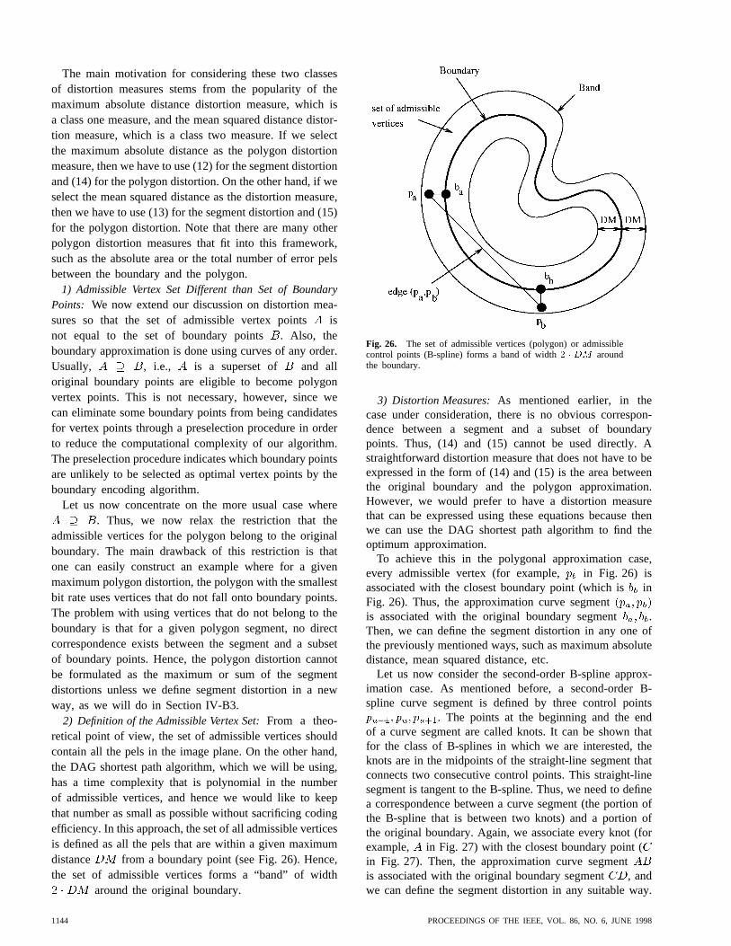
2) Definition of the Admissible Vertex Set:From a theo-retical point of view, the set of admissible vertices shouldcontain all the pels in the image plane. On the other hand,the DAG shortest path algorithm, which we will be using,has a time complexity that is polynomial in the numberof admissible vertices, and hence we would like to keepthat number as small as possible without sacrificing codingefficiency. In this approach, the set of all admissible verticesis defined as all the pels that are within a given maximumdistance from a boundary point (see Fig. 26). Hence,the set of admissible vertices forms a “band” of width
around the original boundary.
Fig. 26. The set of admissible vertices (polygon) or admissiblecontrol points (B-spline) forms a band of width2 � DM aroundthe boundary.
3) Distortion Measures:As mentioned earlier, in thecase under consideration, there is no obvious correspon-dence between a segment and a subset of boundarypoints. Thus, (14) and (15) cannot be used directly. Astraightforward distortion measure that does not have to beexpressed in the form of (14) and (15) is the area betweenthe original boundary and the polygon approximation.However, we would prefer to have a distortion measurethat can be expressed using these equations because thenwe can use the DAG shortest path algorithm to find theoptimum approximation.
To achieve this in the polygonal approximation case,every admissible vertex (for example, in Fig. 26) isassociated with the closest boundary point (which isinFig. 26). Thus, the approximation curve segmentis associated with the original boundary segment .Then, we can define the segment distortion in any one ofthe previously mentioned ways, such as maximum absolutedistance, mean squared distance, etc.
Let us now consider the second-order B-spline approx-imation case. As mentioned before, a second-order B-spline curve segment is defined by three control points
. The points at the beginning and the endof a curve segment are called knots. It can be shown thatfor the class of B-splines in which we are interested, theknots are in the midpoints of the straight-line segment thatconnects two consecutive control points. This straight-linesegment is tangent to the B-spline. Thus, we need to definea correspondence between a curve segment (the portion ofthe B-spline that is between two knots) and a portion ofthe original boundary. Again, we associate every knot (forexample, in Fig. 27) with the closest boundary point (in Fig. 27). Then, the approximation curve segmentis associated with the original boundary segment, andwe can define the segment distortion in any suitable way.
1144 PROCEEDINGS OF THE IEEE, VOL. 86, NO. 6, JUNE 1998
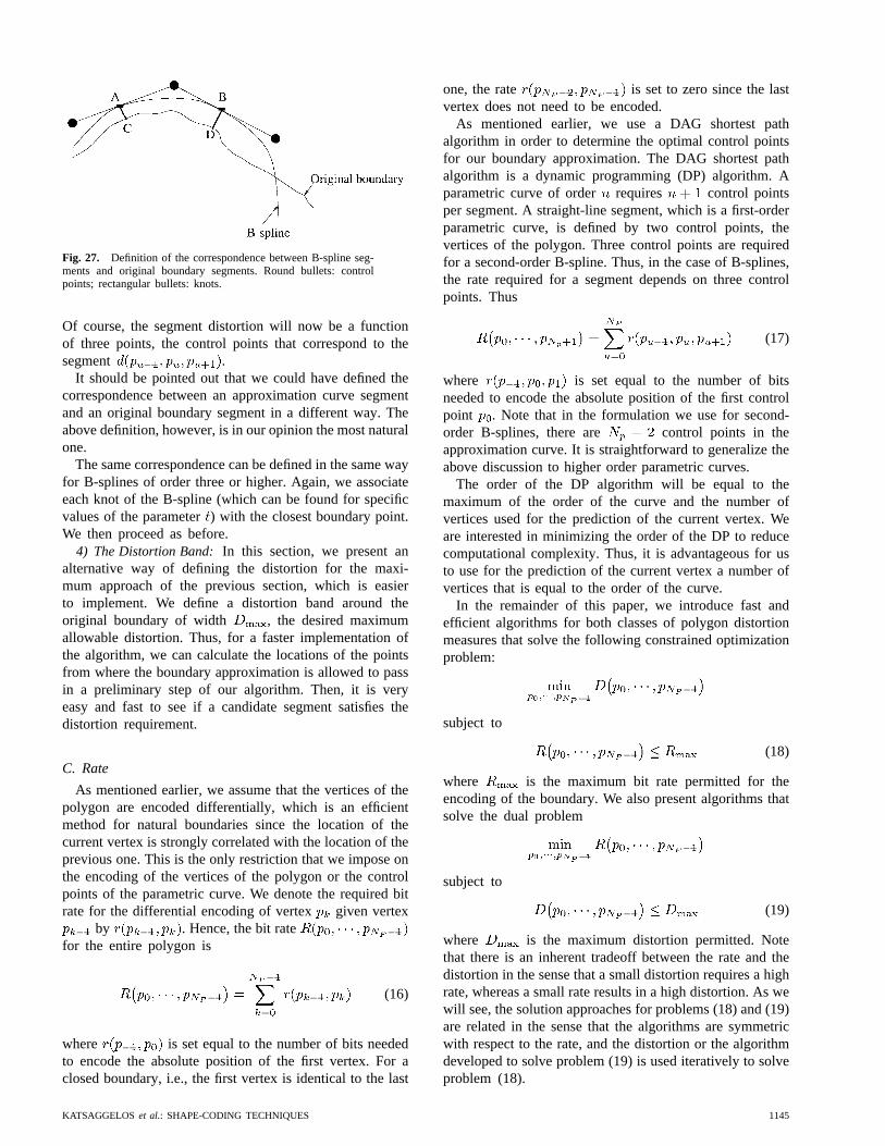
Fig. 27. Definition of the correspondence between B-spline seg-ments and original boundary segments. Round bullets: controlpoints; rectangular bullets: knots.
Of course, the segment distortion will now be a functionof three points, the control points that correspond to thesegment .
It should be pointed out that we could have defined thecorrespondence between an approximation curve segmentand an original boundary segment in a different way. Theabove definition, however, is in our opinion the most naturalone.
The same correspondence can be defined in the same wayfor B-splines of order three or higher. Again, we associateeach knot of the B-spline (which can be found for specificvalues of the parameter) with the closest boundary point.We then proceed as before.
4) The Distortion Band:In this section, we present analternative way of defining the distortion for the maxi-mum approach of the previous section, which is easierto implement. We define a distortion band around theoriginal boundary of width , the desired maximumallowable distortion. Thus, for a faster implementation ofthe algorithm, we can calculate the locations of the pointsfrom where the boundary approximation is allowed to passin a preliminary step of our algorithm. Then, it is veryeasy and fast to see if a candidate segment satisfies thedistortion requirement.
C. Rate
As mentioned earlier, we assume that the vertices of thepolygon are encoded differentially, which is an efficientmethod for natural boundaries since the location of thecurrent vertex is strongly correlated with the location of theprevious one. This is the only restriction that we impose onthe encoding of the vertices of the polygon or the controlpoints of the parametric curve. We denote the required bitrate for the differential encoding of vertex given vertex
by . Hence, the bit ratefor the entire polygon is
(16)
where is set equal to the number of bits neededto encode the absolute position of the first vertex. For aclosed boundary, i.e., the first vertex is identical to the last
one, the rate is set to zero since the lastvertex does not need to be encoded.
As mentioned earlier, we use a DAG shortest pathalgorithm in order to determine the optimal control pointsfor our boundary approximation. The DAG shortest pathalgorithm is a dynamic programming (DP) algorithm. Aparametric curve of order requires control pointsper segment. A straight-line segment, which is a first-orderparametric curve, is defined by two control points, thevertices of the polygon. Three control points are requiredfor a second-order B-spline. Thus, in the case of B-splines,the rate required for a segment depends on three controlpoints. Thus
(17)
where is set equal to the number of bitsneeded to encode the absolute position of the first controlpoint . Note that in the formulation we use for second-order B-splines, there are control points in theapproximation curve. It is straightforward to generalize theabove discussion to higher order parametric curves.
The order of the DP algorithm will be equal to themaximum of the order of the curve and the number ofvertices used for the prediction of the current vertex. Weare interested in minimizing the order of the DP to reducecomputational complexity. Thus, it is advantageous for usto use for the prediction of the current vertex a number ofvertices that is equal to the order of the curve.
In the remainder of this paper, we introduce fast andefficient algorithms for both classes of polygon distortionmeasures that solve the following constrained optimizationproblem:
subject to
(18)
where is the maximum bit rate permitted for theencoding of the boundary. We also present algorithms thatsolve the dual problem
subject to
(19)
where is the maximum distortion permitted. Notethat there is an inherent tradeoff between the rate and thedistortion in the sense that a small distortion requires a highrate, whereas a small rate results in a high distortion. As wewill see, the solution approaches for problems (18) and (19)are related in the sense that the algorithms are symmetricwith respect to the rate, and the distortion or the algorithmdeveloped to solve problem (19) is used iteratively to solveproblem (18).
KATSAGGELOS et al.: SHAPE-CODING TECHNIQUES 1145
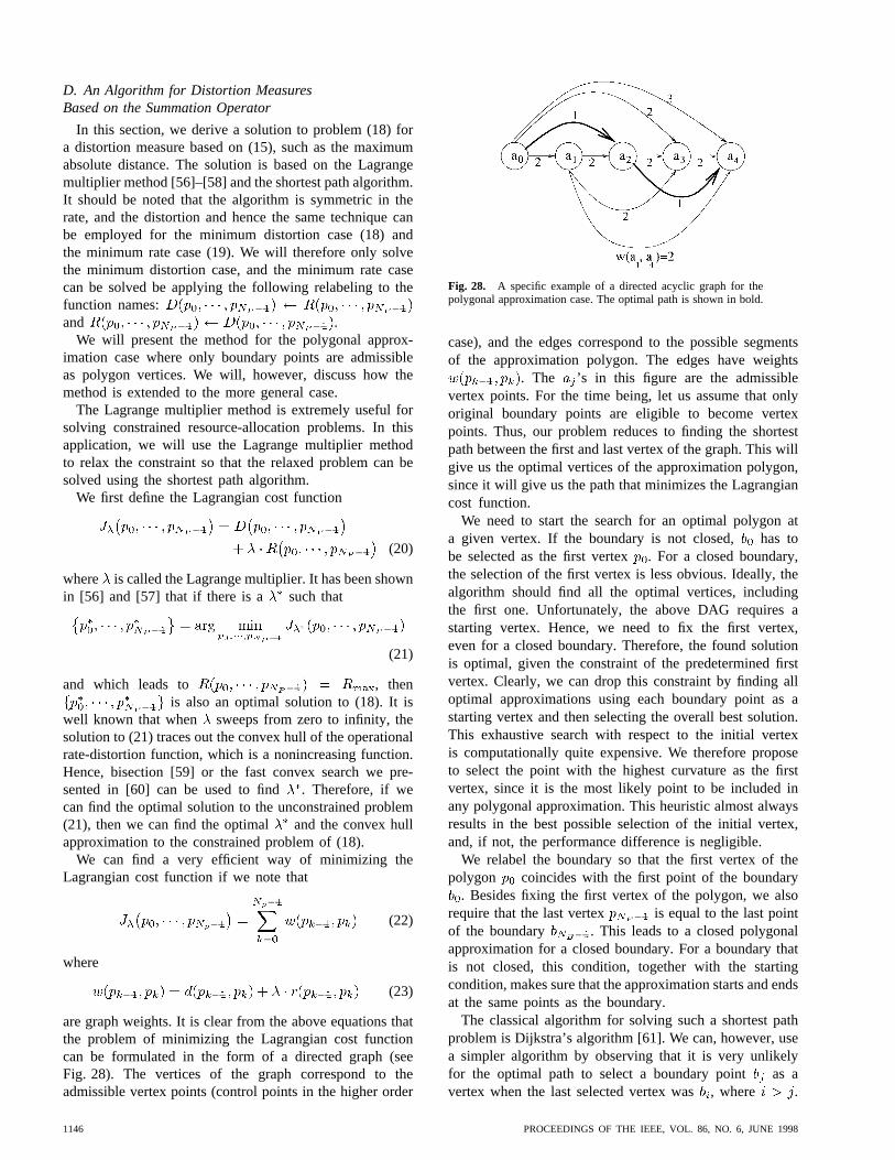
D. An Algorithm for Distortion MeasuresBased on the Summation Operator
In this section, we derive a solution to problem (18) fora distortion measure based on (15), such as the maximumabsolute distance. The solution is based on the Lagrangemultiplier method [56]–[58] and the shortest path algorithm.It should be noted that the algorithm is symmetric in therate, and the distortion and hence the same technique canbe employed for the minimum distortion case (18) andthe minimum rate case (19). We will therefore only solvethe minimum distortion case, and the minimum rate casecan be solved be applying the following relabeling to thefunction names:and .
We will present the method for the polygonal approx-imation case where only boundary points are admissibleas polygon vertices. We will, however, discuss how themethod is extended to the more general case.
The Lagrange multiplier method is extremely useful forsolving constrained resource-allocation problems. In thisapplication, we will use the Lagrange multiplier methodto relax the constraint so that the relaxed problem can besolved using the shortest path algorithm.
We first define the Lagrangian cost function
(20)
where is called the Lagrange multiplier. It has been shownin [56] and [57] that if there is a such that
(21)
and which leads to , thenis also an optimal solution to (18). It is
well known that when sweeps from zero to infinity, thesolution to (21) traces out the convex hull of the operationalrate-distortion function, which is a nonincreasing function.Hence, bisection [59] or the fast convex search we pre-sented in [60] can be used to find . Therefore, if wecan find the optimal solution to the unconstrained problem(21), then we can find the optimal and the convex hullapproximation to the constrained problem of (18).
We can find a very efficient way of minimizing theLagrangian cost function if we note that
(22)
where
(23)
are graph weights. It is clear from the above equations thatthe problem of minimizing the Lagrangian cost functioncan be formulated in the form of a directed graph (seeFig. 28). The vertices of the graph correspond to theadmissible vertex points (control points in the higher order
Fig. 28. A specific example of a directed acyclic graph for thepolygonal approximation case. The optimal path is shown in bold.
case), and the edges correspond to the possible segmentsof the approximation polygon. The edges have weights
. The ’s in this figure are the admissiblevertex points. For the time being, let us assume that onlyoriginal boundary points are eligible to become vertexpoints. Thus, our problem reduces to finding the shortestpath between the first and last vertex of the graph. This willgive us the optimal vertices of the approximation polygon,since it will give us the path that minimizes the Lagrangiancost function.
We need to start the search for an optimal polygon ata given vertex. If the boundary is not closed, has tobe selected as the first vertex. For a closed boundary,the selection of the first vertex is less obvious. Ideally, thealgorithm should find all the optimal vertices, includingthe first one. Unfortunately, the above DAG requires astarting vertex. Hence, we need to fix the first vertex,even for a closed boundary. Therefore, the found solutionis optimal, given the constraint of the predetermined firstvertex. Clearly, we can drop this constraint by finding alloptimal approximations using each boundary point as astarting vertex and then selecting the overall best solution.This exhaustive search with respect to the initial vertexis computationally quite expensive. We therefore proposeto select the point with the highest curvature as the firstvertex, since it is the most likely point to be included inany polygonal approximation. This heuristic almost alwaysresults in the best possible selection of the initial vertex,and, if not, the performance difference is negligible.
We relabel the boundary so that the first vertex of thepolygon coincides with the first point of the boundary
. Besides fixing the first vertex of the polygon, we alsorequire that the last vertex is equal to the last pointof the boundary . This leads to a closed polygonalapproximation for a closed boundary. For a boundary thatis not closed, this condition, together with the startingcondition, makes sure that the approximation starts and endsat the same points as the boundary.
The classical algorithm for solving such a shortest pathproblem is Dijkstra’s algorithm [61]. We can, however, usea simpler algorithm by observing that it is very unlikelyfor the optimal path to select a boundary point as avertex when the last selected vertex was, where .
1146 PROCEEDINGS OF THE IEEE, VOL. 86, NO. 6, JUNE 1998
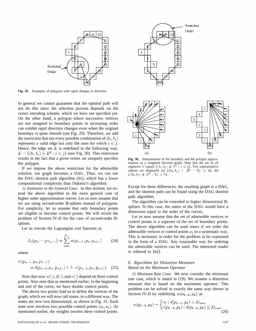
Fig. 29. Examples of polygons with rapid changes in direction.
In general we cannot guarantee that the optimal path willnot do this since the selection process depends on thevertex encoding scheme, which we have not specified yet.On the other hand, a polygon where successive verticesare not assigned to boundary points in increasing ordercan exhibit rapid direction changes even when the originalboundary is quite smooth (see Fig. 29). Therefore, we addthe restriction that not every possible combination ofrepresents a valid edge but only the ones for which .Hence, the edge set is redefined in the following way:
(see Fig. 30). This restrictionresults in the fact that a given vertex set uniquely specifiesthe polygon.
If we impose the above restriction for the admissiblesolution, our graph becomes a DAG. Thus, we can usethe DAG shortest path algorithm [61], which has a lowercomputational complexity than Dijkstra’s algorithm.
1) Extension to the General Case:In this section, we ex-tend the above algorithm to the more general case ofhigher order approximation curves. Let us now assume thatwe are using second-order B-splines instead of polygons.For simplicity, let us assume that only boundary pointsare eligible to become control points. We will revisit theproblem of Section IV-D for the case of second-order B-splines.
Let us rewrite the Lagrangian cost function as
(24)
where
(25)
Note that now , , and depend on three controlpoints. Also note that as mentioned earlier, in the beginningand end of the curve, we have double control points.
The above two points lead us to define the vertices of thegraph, which we will now call states, in a different way. Thestates are now two dimensional, as shown in Fig. 31. Eachstate now involves two possible control points . Asmentioned earlier, the weights involve three control points.
(a) (b)
Fig. 30. Interpretation of the boundary and the polygon approx-imation as a weighted directed graph. Note that the set of allsegmentsE equalsf(bi; bj) 2 B2 : i < jg. Two representativesubsets are displayed. (a)f(b4; bj) 2 B2 : 8j > 4g. (b)f(b8; bj) 2 B2 : 8j > 8g.
Except for these differences, the resulting graph is a DAG,and the shortest path can be found using the DAG shortestpath algorithm.
The algorithm can be extended to higher dimensional B-splines. In this case, the states of the DAG would have adimension equal to the order of the curves.
Let us now assume that the set of admissible vertices orcontrol points is a superset of the set of boundary points.The above algorithm can be used intact if we order theadmissible vertices or control points in a systematic way.This is necessary in order for the problem to be expressedin the form of a DAG. Any reasonable way for orderingthe admissible vertices can be used. The interested readeris referred to [62].
E. Algorithms for Distortion MeasuresBased on the Maximum Operator
1) Minimum Rate Case:We now consider the minimumrate case, which is stated in (19). We assume a distortionmeasure that is based on the maximum operator. Thisproblem can be solved in exactly the same way shown inSection IV-D by redefining as
(26)
KATSAGGELOS et al.: SHAPE-CODING TECHNIQUES 1147
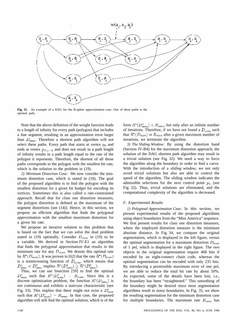
Fig. 31. An example of a DAG for the B-spline approximation case. One of these paths is theoptimal path.
Note that the above definition of the weight function leadsto a length of infinity for every path (polygon) that includesa line segment, resulting in an approximation error largerthan . Therefore a shortest path algorithm will notselect these paths. Every path that starts at vertexandends at vertex and does not result in a path lengthof infinity results in a path length equal to the rate of thepolygon it represents. Therefore, the shortest of all thosepaths corresponds to the polygon with the smallest bit rate,which is the solution to the problem in (19).
2) Minimum Distortion Case:We now consider the min-imum distortion case, which is stated in (18). The goalof the proposed algorithm is to find the polygon with thesmallest distortion for a given bit budget for encoding itsvertices. Sometimes this is also called a rate-constrainedapproach. Recall that for class one distortion measures,the polygon distortion is defined as the maximum of thesegment distortions [see (14)]. Hence, in this section, wepropose an efficient algorithm that finds the polygonalapproximation with the smallest maximum distortion fora given bit rate.
We propose an iterative solution to this problem thatis based on the fact that we can solve the dual problemstated in (19) optimally. Consider in (19) to bea variable. We derived in Section IV-E1 an algorithmthat finds the polygonal approximation that results in theminimum rate for any . We denote this optimal rateby . It was proven in [62] that the rateis a nonincreasing function of , which means that
implies .Thus, we can use bisection [59] to find the optimal
such that . Since this is adiscrete optimization problem, the function isnot continuous and exhibits a staircase characteristic (seeFig. 33). This implies that there might not exist asuch that . In that case, the proposedalgorithm will still find the optimal solution, which is of the
form , but only after an infinite numberof iterations. Therefore, if we have not found a suchthat after a given maximum number ofiterations, we terminate the algorithm.
3) The Sliding Window:By using the distortion band(Section IV-B4) for the maximum distortion approach, thesolution of the DAG shortest path algorithm may result ina trivial solution (see Fig. 32). We need a way to forcethe algorithm along the boundary in order to find a curve.With the introduction of asliding window, we not onlyavoid trivial solutions but also are able to control thespeed of the algorithm. The sliding window indicates theadmissible selections for the next control point (seeFig. 32). Thus, trivial solutions are eliminated, and thecomputational complexity of the algorithm is decreased.
F. Experimental Results
1) Polygonal Approximation Case:In this section, wepresent experimental results of the proposed algorithmsusing object boundaries from the “Miss America” sequence.We first present results for class one distortion measures,where the employed distortion measure is the minimumabsolute distance. In Fig. 34, we compare the originalsegmentation, which is displayed in the left figure, versusthe optimal segmentation for a maximum distortionof 1 pel, which is displayed in the right figure. The twoobjects in the original segmentation require 468 bits ifencoded by an eight-connect chain code, whereas theoptimal segmentation can be encoded with only 235 bits.By introducing a permissible maximum error of one pel,we are able to reduce the total bit rate by about 50%.As expected, some of the details have been lost, i.e.,the boundary has been “straightened.” This smoothing ofthe boundary might be desired since most segmentationalgorithms result in noisy boundaries. In Fig. 35, we showthe resulting segmentation for the minimum distortion casefor multiple boundaries. The maximum rate has
1148 PROCEEDINGS OF THE IEEE, VOL. 86, NO. 6, JUNE 1998
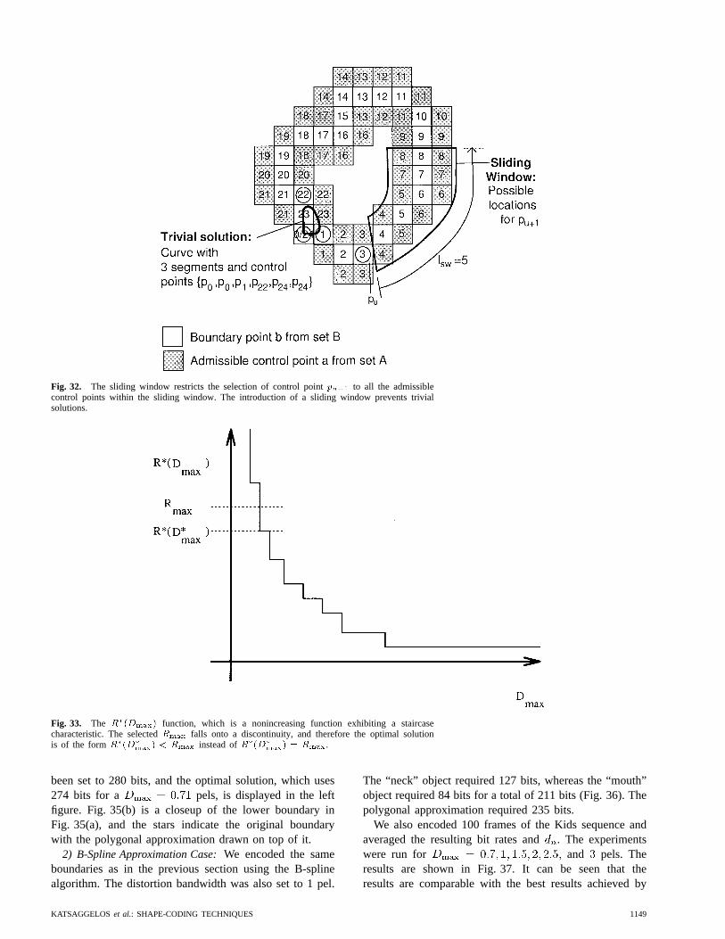
Fig. 32. The sliding window restricts the selection of control pointpu+1 to all the admissiblecontrol points within the sliding window. The introduction of a sliding window prevents trivialsolutions.
Fig. 33. The R�(Dmax) function, which is a nonincreasing function exhibiting a staircasecharacteristic. The selectedRmax falls onto a discontinuity, and therefore the optimal solutionis of the formR�(D�
max) < Rmax instead ofR�(D�
max) = Rmax.
been set to 280 bits, and the optimal solution, which uses274 bits for a pels, is displayed in the leftfigure. Fig. 35(b) is a closeup of the lower boundary inFig. 35(a), and the stars indicate the original boundarywith the polygonal approximation drawn on top of it.
2) B-Spline Approximation Case:We encoded the sameboundaries as in the previous section using the B-splinealgorithm. The distortion bandwidth was also set to 1 pel.
The “neck” object required 127 bits, whereas the “mouth”object required 84 bits for a total of 211 bits (Fig. 36). Thepolygonal approximation required 235 bits.
We also encoded 100 frames of the Kids sequence andaveraged the resulting bit rates and. The experimentswere run for and pels. Theresults are shown in Fig. 37. It can be seen that theresults are comparable with the best results achieved by
KATSAGGELOS et al.: SHAPE-CODING TECHNIQUES 1149
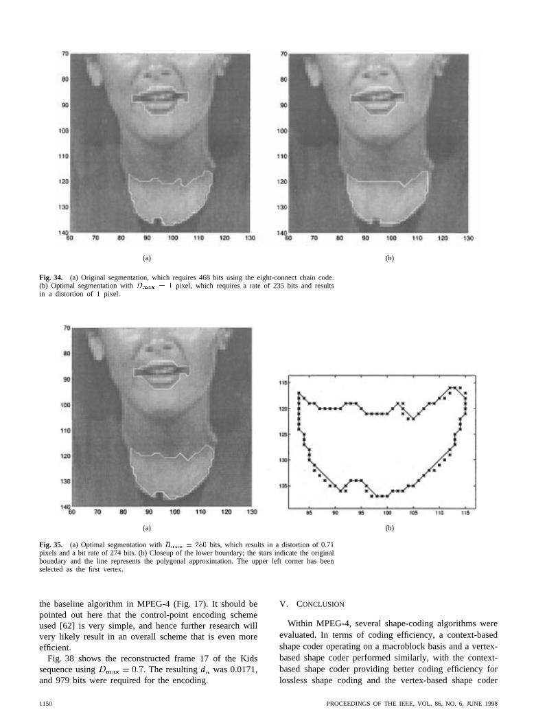
(a) (b)
Fig. 34. (a) Original segmentation, which requires 468 bits using the eight-connect chain code.(b) Optimal segmentation withDmax = 1 pixel, which requires a rate of 235 bits and resultsin a distortion of 1 pixel.
(a) (b)
Fig. 35. (a) Optimal segmentation withRmax = 280 bits, which results in a distortion of 0.71pixels and a bit rate of 274 bits. (b) Closeup of the lower boundary; the stars indicate the originalboundary and the line represents the polygonal approximation. The upper left corner has beenselected as the first vertex.
the baseline algorithm in MPEG-4 (Fig. 17). It should bepointed out here that the control-point encoding schemeused [62] is very simple, and hence further research willvery likely result in an overall scheme that is even moreefficient.
Fig. 38 shows the reconstructed frame 17 of the Kidssequence using . The resulting was 0.0171,and 979 bits were required for the encoding.
V. CONCLUSION
Within MPEG-4, several shape-coding algorithms wereevaluated. In terms of coding efficiency, a context-basedshape coder operating on a macroblock basis and a vertex-based shape coder performed similarly, with the context-based shape coder providing better coding efficiency forlossless shape coding and the vertex-based shape coder
1150 PROCEEDINGS OF THE IEEE, VOL. 86, NO. 6, JUNE 1998
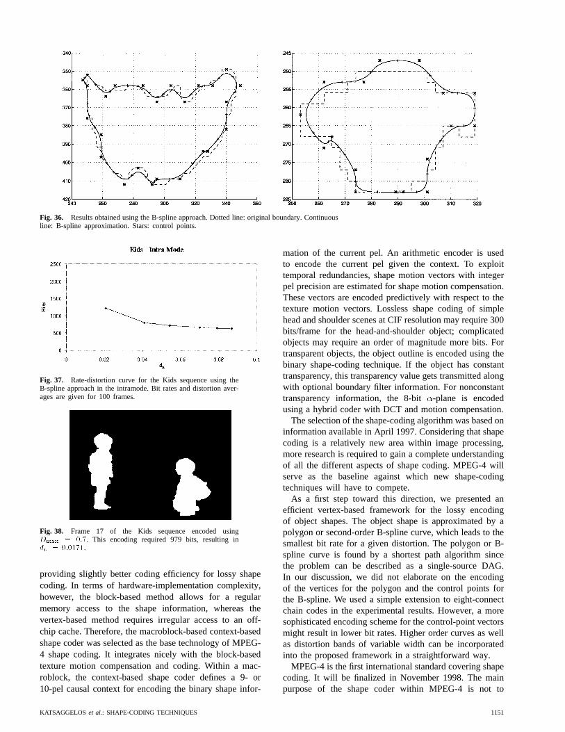
Fig. 36. Results obtained using the B-spline approach. Dotted line: original boundary. Continuousline: B-spline approximation. Stars: control points.
Fig. 37. Rate-distortion curve for the Kids sequence using theB-spline approach in the intramode. Bit rates and distortion aver-ages are given for 100 frames.
Fig. 38. Frame 17 of the Kids sequence encoded usingDmax = 0:7. This encoding required 979 bits, resulting indn = 0:0171.
providing slightly better coding efficiency for lossy shapecoding. In terms of hardware-implementation complexity,however, the block-based method allows for a regularmemory access to the shape information, whereas thevertex-based method requires irregular access to an off-chip cache. Therefore, the macroblock-based context-basedshape coder was selected as the base technology of MPEG-4 shape coding. It integrates nicely with the block-basedtexture motion compensation and coding. Within a mac-roblock, the context-based shape coder defines a 9- or10-pel causal context for encoding the binary shape infor-
mation of the current pel. An arithmetic encoder is usedto encode the current pel given the context. To exploittemporal redundancies, shape motion vectors with integerpel precision are estimated for shape motion compensation.These vectors are encoded predictively with respect to thetexture motion vectors. Lossless shape coding of simplehead and shoulder scenes at CIF resolution may require 300bits/frame for the head-and-shoulder object; complicatedobjects may require an order of magnitude more bits. Fortransparent objects, the object outline is encoded using thebinary shape-coding technique. If the object has constanttransparency, this transparency value gets transmitted alongwith optional boundary filter information. For nonconstanttransparency information, the 8-bit -plane is encodedusing a hybrid coder with DCT and motion compensation.
The selection of the shape-coding algorithm was based oninformation available in April 1997. Considering that shapecoding is a relatively new area within image processing,more research is required to gain a complete understandingof all the different aspects of shape coding. MPEG-4 willserve as the baseline against which new shape-codingtechniques will have to compete.
As a first step toward this direction, we presented anefficient vertex-based framework for the lossy encodingof object shapes. The object shape is approximated by apolygon or second-order B-spline curve, which leads to thesmallest bit rate for a given distortion. The polygon or B-spline curve is found by a shortest path algorithm sincethe problem can be described as a single-source DAG.In our discussion, we did not elaborate on the encodingof the vertices for the polygon and the control points forthe B-spline. We used a simple extension to eight-connectchain codes in the experimental results. However, a moresophisticated encoding scheme for the control-point vectorsmight result in lower bit rates. Higher order curves as wellas distortion bands of variable width can be incorporatedinto the proposed framework in a straightforward way.
MPEG-4 is the first international standard covering shapecoding. It will be finalized in November 1998. The mainpurpose of the shape coder within MPEG-4 is not to
KATSAGGELOS et al.: SHAPE-CODING TECHNIQUES 1151
increase coding efficiency for conventional video, althoughthat has also been shown to accomplish this for some videosequences. Its primary purpose is to enable many new func-tionalities and applications such as object-based data baseaccess, content-based image and video representation, videoediting, efficient storage of movies prior to composition,and more.
ACKNOWLEDGMENT
The authors wish to acknowledge that the materialon MPEG-4 shape coding techniques was primarilycontributed by J. Ostermann, while the rest of the materialwas contributed by the remaining authors. The authors wishto thank C. S. Boon, Matsushita, for providing the data forFigs. 21 and 22 and C. L. Jordan, EPFL, for providingFig. 14. J. S. Shin, SAIT, created Figs. 15–20 during theMPEG meeting in Bristol, U.K., to help the evaluation. M.Rong created Fig. 1. They also wish to thank Y. Wang andA. Reibman for their review of parts of this paper relatedto MPEG-4.
REFERENCES
[1] H. Musmann, M. Hotter, and J. Ostermann, “Object-orientedanalysis-synthesis coding of moving images,”Signal Process.,vol. 1, pp. 117–138, Oct. 1989.
[2] M. Kunt, “Second-generation image coding techniques,”Proc.IEEE, vol. 73, pp. 549–574, Apr. 1985.
[3] R. Koenen, Ed., “Overview of the MPEG-4 standard,” Inter-national Standards Organization, Stockholm meeting, ISO/IECJTC1/SC29/WG11 N1730, July 1997.
[4] W. Li and M. Kunt, “Morphological segmentation appliedto displaced difference coding,”Signal Process., vol. 38, pp.45–56, July 1994.
[5] T. Alpert, V. Baroncini, D. Choi, L. Contin, R. Koenen, andF. P. Peterson, “Subjective evaluation of MPEG-4 codec pro-posals: Methodological approach and test procedures,”SignalProcess., vol. 9, pp. 303–325, May 1997.
[6] N. Diehl, “Object-oriented motion estimation and segmentationin image sequences,”Signal Process., vol. 3, pp. 23–56, 1991.
[7] J. Ostermann, “Object-oriented analysis-synthesis coding basedon the source model of moving rigid 3D objects,”SignalProcess., vol. 6, pp. 143–161, 1994.
[8] M. Hotter, “Optimization and efficiency of an object-orientedanalysis-synthesis coder,”IEEE Trans. Circuits Syst. VideoTechnol., vol. 4, pp. 181–194, Apr. 1994.
[9] J. Ostermann, “Object-oriented analysis-synthesis coding(OOASC) based on the source model of moving flexible 3Dobjects,” IEEE Trans. Image Processing, vol. 3, pp. 705–711,Sept. 1995.
[10] P. Gerken, “Object-based analysis-synthesis coding of imagesequences at very low bit rates,”IEEE Trans. Circuits Syst.,vol. 4, pp. 228–235, June 1994.
[11] G. Martinez, “Shape estimation of articulated objects for object-based analysis-synthesis coding (OBASC),”Signal Process.,vol. 9, pp. 175–199, Mar. 1997.
[12] Y. Wang and O. Lee, “Active mesh—A feature seeking andtracking image sequence representation scheme,”IEEE Trans.Image Processing, vol. 3, pp. 610–624, Sept. 1994.
[13] Y. Altunbasak and A. M. Tekalp, “Closed-form connectivity-preserving solutions for motion compensation using 2-Dmeshes,”IEEE Trans. Image Processing, vol. 6, pp. 1255–1269,Sept. 1997.
[14] CompuServe, Inc., “Graphics interchange format (sm), version89a,” Columbus, OH, July 1990.
[15] “Facsimile coding schemes and coding functions for group 4facsimile apparatus,” CCITT Recommendation T.6, 1994.
[16] “Coded representation of picture and audio informa-tion—Progressive bi-level image compression,” International
Standards Organization, ISO Draft International Standard11544, 1992.
[17] A. N. Netravali and B. Haskell,Digital Pictures, Representationand Compression. New York: Plenum, 1988.
[18] H. Freeman, “On the encoding of arbitrary geometric configura-tions,” IRE Trans. Electron. Comput., vol. EC-10, pp. 260–268,June 1961.
[19] M. Eden and M. Kocher, “On the performance of a contourcoding algorithm in the context of image coding. Part I: Contoursegment coding,”Signal Process., vol. 8, pp. 381–386, July1985.
[20] M. Hotter, “Object-oriented analysis-synthesis coding based onmoving two-dimensional objects,”Signal Process., vol. 2, pp.409–428, Dec. 1990.
[21] G. M. Schuster and A. K. Katsaggelos, “An optimal segmen-tation encoding scheme in the rate distortion sense,” inProc.IEEE Int. Symp. Circuits and Systems, 1996, pp. 640–643.
[22] G. M. Schuster and A. K. Katsaggelos, “An optimal boundaryencoding scheme in the rate distortion sense,”IEEE Trans.Image Processing, vol. 7, pp. 13–26, Jan. 1998.
[23] K. J. O’Connell, “Object-adaptive vertex-based shape codingmethod,” IEEE Trans. Circuits Syst. Video Technol., vol. 7, pp.251–255, Feb. 1997.
[24] C. T. Zahn and R. Z. Roskies, “Fourier descriptors for planeclosed curves,”IEEE Trans. Comput., vol. C-21, pp. 269–281,Mar. 1972.
[25] P. Salembier, F. Marques, and A. Gasull, “Coding of partitionsequences,” inVideo Coding, L. Torres and M. Kunt, Eds.Boston, MA: Kluwer, 1996, pp. 125–170.
[26] J. Saghri and H. Freeman, “Analysis of the precision of gen-eralized chain codes for the representation of planar curves,”IEEE Trans. Pattern Anal. Machine Intell., vol. PAMI-3, pp.533–539, Sept. 1981.
[27] J. Koplowitz, “On the performance of chain codes for quanti-zation of line drawings,”IEEE Trans. Pattern Anal. MachineIntell., vol. PAMI-3, pp. 180–185, Mar. 1981.
[28] D. Neuhoff and K. Castor, “A rate and distortion analysis ofchain codes for line drawings,”IEEE Trans. Inform. Theory,vol. IT-31, pp. 53–68, Jan. 1985.
[29] T. Kaneko and M. Okudaira, “Encoding of arbitrary curvesbased on the chain code representation,”IEEE Trans. Commun.,vol. COM-33, pp. 697–707, July 1985.
[30] R. Prasad, J. W. Vieveen, J. H. Bons, and J. C. Arnbak,“Relative vector probabilities in differential chain coded line-drawings,” in Proc. IEEE Pacific Rim Conf. Communication,Computers and Signal Processing, Victoria, Canada, June 1989,pp. 138–142.
[31] P. Nunes, F. Pereira, and F. Marques, “Multi-grid chain codingof binary shapes,” inProc. Special Session on Shape Coding,ICIP’97, Santa Barbara, CA, 1997, pp. 114–117.
[32] T. Ozcelik and A. K. Katsaggelos, Very Low Bit Rate VideoCoding Based on Statistical Spatio-Temporal Prediction ofMotion, Segmentation and Intensity Fields, inVideo DataCompression for Multimedia Computing,H. H. Li, S. Sun, andH. Derin, Eds. Norwell, MA: Kluwer, 1997, pp. 313–353.
[33] A. K. Jain,Fundamentals of Digital Image Processing. Engle-wood Cliffs, NJ: Prentice-Hall, 1989.
[34] P. van Otterloo,A Contour-Oriented Approach for Shape Anal-ysis. Hertfordshire, UK: Prentice-Hall, 1991.
[35] N. Brady, F. Bossen, and N. Murphy, “Context-based arithmeticencoding of 2D shape sequences,” inProc. Special Session onShape Coding, ICIP97, Santa Barbara, CA, 1997, pp. I-29–32.
[36] N. Yamaguchi, T. Ida, and T. Watanabe, “A binary shapecoding method using modified MMR,” inProc. Special Sessionon Shape Coding, ICIP97, Santa Barbara, CA, 1997, pp. I-504–508.
[37] S. Lee, D. Cho, Y. Cho, S. Son, E. Jang, and J. Shin, “Binaryshape coding using 1-D distance values from baseline,” inProc.Special Session on Shape Coding, ICIP97, Santa Barbara, CA,1997, pp. I-508–511.
[38] J. Ostermann, “Methodologies used for evaluation of videotools and algorithms in MPEG-4,”Signal Process., vol. 9, pp.343–365, 1997.
[39] T. Sikora, S. Bauer, and B. Makai, “Efficiency of shape-adaptive transforms for coding of arbitrarily shaped imagesegments,”IEEE Trans. Circuits Syst. Video Technol., vol. 5,pp. 254–258, June 1995.
1152 PROCEEDINGS OF THE IEEE, VOL. 86, NO. 6, JUNE 1998
[40] J. Kim and B. L. Evans, “Predictive shape coding using genericpolygon approximation,” inProc. ISCAS’98, Monterrey, CA, tobe published.
[41] T. Chen, C. T. Swain, and B. G. Haskell, “Coding of subregionsfor content-based scalable video,”IEEE Trans. Circuits Syst.Video Technol., vol. 7, pp. 256–260, Feb. 1997.
[42] P. M. Kuhn and W. Stechele, “Complexity analysis of theemerging MPEG-4 standard as a basis for VLSI implemen-tation,” in Proc. SPIE Visual Communications and Image Pro-cessing,San Jose, CA, 1998, vol. 3309, pp. 498-509.
[43] P. Kuhn, “A portable instruction level profiler for complex-ity analysis documentation,” International Standards Organi-zation, ISO/IEC JTC1/WG11 MPEG96/M0921, Tampere, Fin-land, 1996.
[44] J. Arnold and M. Frater, International Standards Organiza-tion, ISO/IEC JTC1/SC29/WG11, Bristol meeting, Apr. 1997,private communication.
[45] J. Brailean, “Report of Ad-Hoc Group on Error Resilience,” In-ternational Standards Organization, ISO/IEC JTC1/SC29/WG11M2113, Bristol meeting, Apr. 1997.
[46] T. Ebrahimi, Ed., “MPEG-4 video verification model ver-sion 8.0,” International Standards Organization, ISO/IECJTC1/SC29/WG11 MPEG97/N1796, July 1997.
[47] T. Ebrahimi, Ed., MPEG-4 video verification modelversion 5, International Standards Organization, ISO/IECJTC1/SC29/WG11 MPEG97/N1469, Nov. 1996.
[48] J. W. Stroming, Y. Kang, T. S. Huang, and S. M. Kang,“New architectures for modified MMR shape coding,” inProc.ISCAS’97, Hong Kong, June 1997, pp. 1205–1208.
[49] W. Chen and M. Lee, “Alpha-channel compression in videocoding,” in Proc. Special Session on Shape Coding, ICIP’97,Santa Barbara, CA, 1997, pp. 500–503.
[50] F. W. Meier, “An efficient shape coding scheme using B-splineswhich is optimal in the rate-distortion sense,” master’s thesis,Northwestern University, Evanston, IL, June 1997.
[51] F. W. Meier, G. M. Schuster, and A. K. Katsaggelos, “Anefficient boundary encoding scheme which is optimal in therate-distortion sense,” inProc. Int. Conf. Image Processing,Santa Barbara, CA, 1997, pp. II-9–12.
[52] F. W. Meier, G. M. Schuster, and A. K. Katsaggelos, “An ef-ficient boundary encoding scheme using B-spline curves whichis optimal in the rate-distortion sense,” inProc. 2nd ErlangenSymp., Advances in Digital Image Communication, Erlangen,Germany, Apr. 1997, pp. 75–84.
[53] J. D. Foley, A. van Dam, S. Feiner, and J. Hughes,ComputerGraphics: Principles and Practice. Reading, MA: Addison-Wesley, 1990, pp. 478–516.
[54] G. M. Schuster and A. K. Katsaggelos, “An optimal lossy seg-mentation encoding scheme,” inProc. SPIE Conf. Visual Com-munications and Image Processing, Mar. 1996, pp. 1050–1061.
[55] G. M. Schuster and A. K. Katsaggelos, “An optimal segmen-tation encoding scheme in the rate-distortion sense,” inProc.Int. Symp. Circuits and Systems, Atlanta, GA, May 1996, vol.2, pp. 640–643.
[56] H. Everett, “Generalized Lagrange multiplier method for solv-ing problems of optimum allocation of resources,”Oper. Res.,vol. 11, pp. 399–417, 1963.
[57] Y. Shoham and A. Gersho, “Efficient bit allocation for anarbitrary set of quantizers,”IEEE Trans. Acoust., Speech, SignalProcessing, vol. 36, pp. 1445–1453, Sept. 1988.
[58] K. Ramchandran, A. Ortega, and M. Vetterli, “Bit allocationfor dependent quantization with applications to multiresolutionand MPEG video coders,”IEEE Trans. Image Processing, vol.3, pp. 533–545, Sept. 1994.
[59] C. F. Gerald and P. O. Wheatley,Applied Numerical Analysis,4th ed. Reading, MA: Addison-Wesley, 1990.
[60] G. M. Schuster and A. K. Katsaggelos, “Fast and efficientmode and quantizer selection in the rate distortion sense forH.263,” in Proc. SPIE Conf. Visual Communications and ImageProcessing, Mar. 1996, pp. 784–795.
[61] T. Cormen, C. Leiserson, and R. Rivest,Introduction to Algo-rithms. New York: McGraw-Hill, 1991.
[62] G. M. Schuster and A. K. Katsaggelos,Rate-Distortion BasedVideo Compression, Optimal Video Frame Compression andObject Boundary Encoding. Norwell, MA: Kluwer, 1997.
[63] J. Ostermann, Ed., “Core experiments on MPEG-4 videoshape coding,” International Standards Organization,
ISO/IEC/JTC1/SC29/WG11 N1584, Seville meeting, Feb.1997.
[64] M. Hotter, “Objectorientiere analyze-synthese codierungbasierend auf dem modell bewegter, zweidimensinalenobjekte,” Ph.D. dissertation, Universit¨at Hannover, Fortschritt-Berichte VDI, Hannover, Germany, 1992.
[65] C. L. Jordan, F. Bossen, and T. Ebrahimi, “Scalable shaperepresentation for content based visual data compression,” inProc. Special Session on Shape Coding, ICIP97, Santa Barbara,CA, 1997, pp. 512–515.
[66] C. S. Boon, private communications, July 1995.
Aggelos K. Katsaggelos(Fellow, IEEE) re-ceived the diploma degree in electrical and me-chanical engineering from the Aristotelian Uni-versity of Thessaloniki, Thessaloniki, Greece,in 1979 and the M.S. and Ph.D. degrees inelectrical engineering from the Georgia Instituteof Technology, Atlanta, GA, in 1981 and 1985,respectively.
In 1985, he joined the Department of Electri-cal Engineering and Computer Science at North-western University, Evanston, IL, where he is
currently a Professor and the Ameritech Chair of Information Technology.During the 1986–1987 academic year, he was an Assistant Professor withthe Department of Electrical Engineering and Computer Science, Polytech-nic University, Brooklyn, NY. His current research interests include imageand video recovery, video compression, motion estimation, boundary en-coding, computational vision, and multimedia signal processing. He was anArea Editor forGraphical Models and Image Processing(1992–1995). Heis the editor ofDigital Image Restoration(Heidelberg, Germany: Springer-Verlag, 1991), coauthor ofRate-Distortion Based Video Compression(Norwell, MA: Kluwer, 1997), and coeditor ofRecovery Techniques forImage and Video Compression,(Norwell, MA: Kluwer, to be published).He was the General Chairman of the 1994 Visual Communications andImage Processing Conference (Chicago, IL).
Dr. Katsaggelos is an Ameritech Fellow, a member of the AssociateStaff, Department of Medicine, Evanston Hospital, and a member ofthe International Society for Optical Engineering. He is a member ofthe Steering Committees of IEEE TRANSACTIONS ON MEDICAL IMAGING
and IEEE TRANSACTIONS ON IMAGE PROCESSING; the IEEE TechnicalCommittees on Visual Signal Processing and Communications, Imageand Multidimensional Signal Processing, and Multimedia Signal Pro-cessing; the Technical Chamber of Commerce of Greece; and SigmaXi. He was an Associate Editor of IEEE TRANSACTIONS ON SIGNAL
PROCESSING (1990–1992) and is currently the Editor-In-Chief of IEEESIGNAL PROCESSINGMAGAZINE. He will be the Technical Program Cochairof the 1998 IEEE International Conference on Image Processing (Chicago,IL).
Lisimachos P. Kondi (Student Member, IEEE)was born in Athens, Greece, on June 23,1971. He received the diploma degree fromthe Aristotelian University of Thessaloniki,Thessaloniki, Greece, in 1994 and the M.S.degree from Northwestern University, Evanston,IL, in 1996, both in electrical engineering. He ispursuing the Ph.D. degree in the Departmentof Electrical and Computer Engineering atNorthwestern University.
His research interests include very-low-bit-rate scalable video compression and shape coding.
KATSAGGELOS et al.: SHAPE-CODING TECHNIQUES 1153
Fabian W. Meier was born on July 21, 1968, inZurich, Switzerland. He received the B.S. degreein electrical engineering from the RapperswilSchool of Engineering, Switzerland, in 1995and the M.S. degree in electrical engineeringfrom Northwestern University, Evanston, IL, in1997.
Since 1997, he has been with SiliconGraphics, Inc., Mountain View, CA, wherehe is involved in the design of a videocodec application-specific integrated circuit for
professional high-definition television applications. Before receiving theundergraduate degree, he conducted solar-energy research in Switzerland.His current research interests include image compression, shape coding,three-dimensional graphics, and agent technology.
Jorn Ostermann studied electrical engineeringand communications engineering at the Univer-sity of Hannover, Germany, and Imperial Col-lege London, England, respectively. He receivedthe Dipl.-Ing. and Dr.-Ing. from the Universityof Hannover in 1988 and 1994, respectively.
From 1988 to 1994, he was a Research Assis-tant with the Institut fur Theoretische Nachrich-tentechnik conducting research in low-bit-rateand object-based analysis-synthesis video cod-ing. During 1994–1995, he was with the Visual
Communications Research Department at Bell Labs. Since 1996, he hasbeen with the Image Processing and Technology Research Lab withinAT&T Labs-Research, Red Bank, NJ. From 1993 to 1994, he wasChairman of the European COST 211 sim group coordinating research inlow-bit-rate video coding. Within MPEG-4, he organized the evaluationof video tools to start defining the standard. Currently, he is Chairman ofthe Ad Hoc Group on Coding of Arbitrarily-Shaped Objects in MPEG-4 Video, defining the content-based video-coding aspects of MPEG-4.His current research interests are video coding, computer vision, three-dimensional modeling, face animation, and coarticulation of acoustic andvisual speech.
Guido M. Schuster (Member, IEEE) receivedthe Ing HTL degree in elektronik, Mess-, undRegeltechnik from the Neu Technikum Buchs(NTB), Buchs, St. Gallen, Switzerland, in 1990.He received the M.S. and Ph.D. degrees inelectrical engineering from Northwestern Uni-versity, Evanston, IL, in 1992 and 1996, respec-tively.
In 1996, he joined the Network Systems Divi-sion of U.S. Robotics (now the Carrier SystemsBusiness Unit of 3Com), Mount Prospect, IL,
where he cofounded the Advanced Technologies Research Center. He hasreceived several patents in fields ranging from adaptive control over videocompression to Internet telephony. He is the coauthor ofRate-DistortionBased Video Compression(Norwell, MA: Kluwer, 1997). His currentresearch interests are operational rate-distortion theory and networkedmultimedia.
At the NTB, Dr. Schuster received the Gold Medal for Academic Ex-cellence and won the First Annual Landis & Gyr Fellowship Competition.
1154 PROCEEDINGS OF THE IEEE, VOL. 86, NO. 6, JUNE 1998
Related Documents