MPC for stable linear systems with model uncertainty

Available online at www.sciencedirect.com

Automatica 39 (2003) 569–583

www.elsevier.com/locate/automatica

MPC for stable linear systems with model uncertainty�

Marco A. Rodrigues, Darci Odloak∗

Department of Chemical Engineering, University of Sao Paulo, Av Prof Luciano Gualberto, trv 3 380, C.P. 61548,Sao Paulo 05508-900, Brazil

Received 13 December 2000; received in revised form 9 March 2002; accepted 29 July 2002

Abstract

In this paper, we developed a model predictive controller, which is robust to model uncertainty. Systems with stable dynamics aretreated. The paper is mainly focused on the output-tracking problem of a system with unknown steady state. The controller is based on astate-space model in which the output is represented as a continuous function of time. Taking advantage of this particular model form,the cost functions is de2ned in terms of the integral of the output error along an in2nite prediction horizon. The model states are assumedperfectly known at each sampling instant (state feedback). The controller is robust for two classes of model uncertainty: the multi-modelplant and polytopic input matrix. Simulations examples demonstrate that the approach can be useful for practical application.? 2003 Elsevier Science Ltd. All rights reserved.

Keywords: Model predictive control; Robust stability; Robust control; State-feedback

1. Introduction

In the model predictive control strategy, at each sam-ple step, an optimal sequence of control inputs, whichminimizes an open loop cost function, is computed. Theoptimization problem also includes hard constraints onthe inputs and soft constraints on the outputs or states. Inthe output-tracking problem, the cost function is de2ned asthe sum of the squared di9erences between the predictedoutput at sampling instants and the output reference value.The weighted sum of the inputs is also included.A modeling approach frequently adopted in model predic-

tive controller (MPC) considers a discrete-time state-spacemodel in the incremental form (Lee, Morari, & Garcia,1994)

[x]k+1 = A[x]k + BAuk ; (1)

[y]k = C[x]k ; (2)

� This paper was not presented at any IFAC meeting. This paper wasrecommended for publication in revised form by Associate Editor FrankAllgCower under the direction of Editor Sigurd Skogestad.

∗ Corresponding author. Tel.: +55-11-3813-9824; fax: +55-11-3813-2380.

E-mail addresses: [email protected] (M. A. Rodrigues),[email protected] (D. Odloak).

where x∈Rnx is the vector of states, u∈Rnu is the vectorof inputs, Auk = uk − uk−1 is the input increment, k is thepresent time step and y∈Rny is the vector of outputs. A; Band C are matrices with appropriate dimensions. In the MPCliterature, robustness is sought considering certain classesof model uncertainty. From the practical point of view, thefollowing classes can be considered relevant:(i)Multi-model system (Badgwell, 1997), where the true

matrices (A; B; C) of (1) and (2) are unknown but lie ina set {Aj; Bj; Cj}; j = 1; 2; : : : ; L. Each j corresponds to aparticular operating point of the system.(ii) Polytopic system, where matrices (A; B; C) are

assumed to lie in a polytopic set (Kothare, Balakrishnan,& Morari, 1996)

(A; B; C) =L∑i=1

�i(Ai; Bi; Ci);

L∑j=1

�j = 1; �j¿ 0; j = 1; : : : ; L:

A particular sub-class of this kind of model uncertainty as-sumes that uncertainty concentrates on the input distributionmatrix. In this case, B is such that

B(�) =L∑j=1

�jBj;L∑j=1

�j = 1; �j¿ 0; j = 1; : : : ; L;

0005-1098/03/$ - see front matter ? 2003 Elsevier Science Ltd. All rights reserved.doi:10.1016/S0005-1098(02)00176-0

mailto:[email protected]

mailto:[email protected]

570 M.A. Rodrigues, D. Odloak /Automatica 39 (2003) 569–583

and A and C are assumed to be known and invariant (Lee& Cooley, 2000).In the design ofMPC, robust stability is an important issue

(Mayne, Rawlings, Rao, & Scokaert, 2000; Morari & Lee,1999). The target is to design a controller that is stable inde-pendent of the operating conditions, which usually alters theprocess model. For the nominal case, where only the mostlikely model is considered by the controller, there are severalmethods to obtain a stable MPC. A popular approach consid-ers that the output and input horizons are 2nite, and stabilityis obtained through the inclusion of a terminal state con-straint (Keerthi & Gilbert, 1988; Meadows, Henson, Eaton,& Rawlings, 1995; Polak & Yang, 1993). This methodcannot be usually extended to the robust output-trackingproblem because the terminal constraint cannot be simulta-neously satis2ed by all the possible process models. Anotherusual method to obtain a stable MPC is based on an in2niteoutput horizon (Rawlings & Muske, 1993). For stable sys-tems, the in2nite horizon open loop cost can be expressedas a 2nite horizon cost with the inclusion of a terminal statepenalty, which has to be computed through the solution ofa Lyapunov equation. The extension of this approach to therobust multi-model MPC was proposed by Badgwell (1997)with the inclusion of contracting constraints for the costsassociated with the possible plants. In that method, it wasassumed that, for the computed input sequence, the stategoes to zero at in2nite time for all possible plant models.This assumption is not usually true for the output-trackingproblem where, in most of the cases, the system steady stateis not known. To overcome this problem, Ralhan (1999)proposed a two-stage approach. In the upper stage, targetsfor the inputs are searched such that the o9set in the systemoutput is minimized. These targets are passed to the sec-ond stage for the robust dynamic optimization. Althoughrobust stability is not guaranteed, the author showed thatif the system reaches a steady state, it will be the correctsteady state. Kothare et al. (1996) proposed a min–maxpredictive control algorithm where the worst-case optimallinear state feedback is treated as an LMI problem. The ap-proach was extended by Lu and Arkun (2000) to polytopiclinear parameter-varying systems and for the schedulingMPC problem. Rodrigues and Odloak (2000) proposed asolution to the output feedback robust MPC through the ex-plicit inclusion of a Lyapunov-type inequality constraint inthe control optimization problem. Lee and Cooley (2000)extended the approach of Rawlings and Muske (1993) tothe robust regulator problem of a system with time-varyinginput matrix.The method proposed in this work can be considered as a

further extension of the in2nite horizon MPC (IHMPC) ofRawlings and Muske (1993) to systems with model uncer-tainty. When compared to the method of Badgwell (1997)we can identify the following improvements:

• The state-space model on which the controller is basedimproves the system representation usually adopted in

the MPC literature. With this model, for a 2nite controlhorizon, the in2nite output horizon MPC cost functioncan be integrated explicitly. The approach becomes moreeLcient as the computation of the control sequence doesnot include the solution of the Lyapunov equation tocompute the terminal state penalty. The on-line solu-tion of this equation may be time consuming for largesystems.

• The usual MPC cost function is modi2ed to guaranteethat the cost remains bounded for all possible models ofthe process. This is done through the inclusion of slackvariables in the output error. With this approach, weprove that the robust controller drives the true plant tothe desired reference values.

• This work overcomes one of the major barriers to thepractical implementation of robust MPC: the need toknow the system steady state. Hence, it can be applied tothe output-tracking problem and to the regulator problemwith unknown disturbances.

The paper is organized as follows. In Section 2, we sum-marize the in2nite horizon control problem from the pointof view of the state-space model with continuous-time out-put prediction (Rodrigues & Odloak, 2001). This model al-lows a simple solution to the in2nite horizon problem. InSection 3, the IHMPC is extended to plants with multipleoperating points and plants with uncertainty in the input ma-trix. In Section 4, simulations of two typical process controlsystems illustrate the application of the robust controller.Finally, Section 5 concludes the paper.

2. Revisited IHMPC

MPC is usually based on a discrete state-space model asshown in Eqs. (1) and (2). In the output-tracking problem,the IHMPC cost can be de2ned as follows:

Jk;∞ =∞∑j=0

eTk+jQek+j +m−1∑j=0

AuTk+jRAuk+j; (3)

where ek+j = y(k + j) − r(j); y(k + j) is the output pre-diction at time instant k + j made at time k; r is the desiredoutput reference, m is the control horizon, Q∈Rny×ny andR∈Rnu×nu are positive de2nite weighting matrices. Thecontroller that is based on the minimization of the abovecost function corresponds to the IHMPC (Rawlings &Muske, 1993) for the output-tracking case. Most of the in2-nite horizon controllers reduce to 2nite horizon controllersby de2ning a terminal state penalty NQ. For the cost de2nedin (3) such a terminal penalty is computed by the followingLyapunov equation (Muske & Rawlings, 1993; Lee &Cooley, 2000):

NQ = CTQC + AT NQA; (4)

where matrices A and C are related to the stable modesof the system and can be obtained from model matrices A

M.A. Rodrigues, D. Odloak /Automatica 39 (2003) 569–583 571

and C. With the terminal penalty, the cost de2ned in (3)reduces to

Jk;∞ =m−1∑j=0

eTk+jQek+j + eTk+m

NQek+m

+m−1∑j=0

AuTk+jRAuk+j: (5)

Industrial controllers usually provide the operator with thefacility to include or exclude an output from the computationof the control action. This is particularly useful when theoperator detects a faulty output measurement. In this case,matrix A is altered and (4) has to be solved in real time todetermine NQ that corresponds to the set of valid outputs. Inthis paper, a di9erent approach is followed to represent thein2nite horizon cost. The approach is based on a state-spacemodel in which the states are the coeLcients of the outputprediction function. A simple example illustrates the formof such a model:

Example 1. Consider the system represented by the transferfunction in

G(s) =1

s(10s+ 1)2:

The corresponding step response of this system is S(t) =−20 + 20e−0:1t + t + te−0:1t . With sampling time T = 1, astate-space model corresponding to Eqs. (1) and (2) for thissystem can be written as follows:

[x]k+1 =

1 0 1 0

0 0:9048 0 0:9048

0 0 1 0

0 0 0 0:9048

[x]k

+

−19

19:0016

1

0:9048

Auk ; (6)

[y(k + t)]k = [1 e−0:1t t te−0:1t][x]k : (7)

Examining (7), we observe that the output matrix dependson the continuous time t. Output matrix C in (2) of theconventional discrete-time model could be obtained fromthe output matrix presented in (7) as follows:

C = [1 e−0:1t t te−0:1t]t=0 = [1 1 0 0]:

We note that in (6) there are four states, while the transferfunction that originated from the model can be representedby a model with three states. The fourth state is related to theincremental form of the input (Auk) in (6), which createsan additional integrating state.

Next, we particularize this model formulation to systemswith single non-integrating poles. After the model presen-tation, we will review the IHMPC that corresponds to thisstate-space model (Rodrigues & Odloak, 2001).We can generalize the procedure of Example 1 to develop

a state-space model corresponding to an SISO system inwhich the relation between input u and output y is describedby the transfer function model

y(s)u(s)

=b0 + b1s+ b2s2 + · · ·+ bnbsnb1 + a1s+ a2s2 + · · ·+ anasna ;

where {na; nb∈N | nb¡na}. If we assume that the systemhas only stable poles with single multiplicity, the systemstep response at time t can be written as follows:

S(t) = d0 +na∑l=1

[ddl ]erlt ;

where rl; l= 1; 2; : : : ; na, are the poles of the system. Co-eLcients d0; ddi ; : : : ; d

dna are obtained by partial fractions ex-

pansion of the system transfer function. For a sampling timeT and using the model notation introduced in (1) and (2),the following equations can be written at time step k for thestates and for the output at time instant kT + t:

[x1]k+1 = [x1]k + d0 Auk ;

[xl+1]k+1 = erlT [xl+1]k + d

dl erlT Auk ; l= 1; 2; : : : ; na;

[y(kT + t)]k = [x1]k +na∑l=1

[xl+1]kerlt :

Analogously, for an MIMO stable system with nu inputs andny outputs, the transfer function relating input uj to outputyi is represented by

Gi;j(s) =bi; j;0 + bi; j;1s+ bi; j;2s2 + · · ·+ bi; j;nbsnb1 + ai; j;1s+ ai; j;2s2 + · · ·+ ai; j;nasna :

The prediction equation for output yi takes the form

[yi(kT + t)]k

=[xi]k +nu∑j=1

na∑l=1

[x(i−1)nu na+( j−1)na+ny+l]keri; j; lt ;

i = 1; : : : ; ny; (8)

where

[xi]k+1 = [xi]k +nu∑j=1

d0i; j[Auj]k (9)

[x(i−1)nu na+( j−1)na+ny+l]k+1

=eri; j; lT [x(i−1)nu na+( j−1)na+ny+l]k + di;j; leri; j; lT [Auj]k ;

i = 1; : : : ; ny; j = 1; : : : ; nu; l= 1; : : : ; na: (10)

For the development of the IHMPC, it is convenient toseparate the state vector into two components as follows:x = [(xs)T (xd)T]T where xs = [x1 · · · xny]T; xs ∈Rny and


xd=[xny+1 xny+2 · · · xny(nu na+1)]T; xd ∈Cny nu na. For stablesystems, xs can be interpreted as the output predicted steadystate. This interpretation is justi2able if we use Eq. (8) tocompute the limit of the output when time tends to in2nite:limt→∞ yi(kT + t) = [xd]k .With these de2nitions and using vector notation, Eq. (8)

can be written as

[y(kT + t)]k = [xs]k +�(t)[xd]k ; (11)

where

�(t) =

1(t) 0 · · · 0

0 2(t) · · · 0

......

. . ....

0 0 · · · ny(t)

;

�(t)∈Cny×nd; (12)

nd= ny nu na;

�i(t) = [eri; 1; 1t · · · eri; 1; nat · · · eri; nu; 1t · · · eri; nu; nat];i = 1; 2; : : : ; ny; �i ∈Cnd:

Analogously, Eqs. (9) and (10) become

[xs]k+1 = [xs]k + D0Auk ; (13)

[xd]k+1 = F[xd]k + D

dFNAuk ; (14)

where

D0 =

d01;1 · · · d01; nu...

. . ....

d0ny;1 · · · d0ny;nu

; D0 ∈Rny×nu;

F = diag(er1; 1; 1T · · · er1; 1; naT · · · er1; nu; 1T · · · er1; nu; naT · · ·· · · erny; 1; 1T · · · erny; 1; naT · · · erny; nu; 1T · · · erny; nu; naT );

F ∈Cnd×nd;

Dd = diag(dd1;1;1 · · ·dd1;1; na · · ·dd1; nu;1 · · ·dd1; nu;na · · ·· · ·ddny;1;1 · · ·ddny;1; na · · ·ddny;nu;1 · · ·ddny;nu;na);

Dd ∈Cnd×nd;

N =

J1

J2

...

Jny

; N ∈Rnd×nu;

Ji =

1 0 0 · · · 0

1 0 0 · · · 0

......

... · · · ...

1 0 0 · · · 0

0 1 0 · · · 0

0 1 0 · · · 0

......

... · · · ...

0 1 0 · · · 0

...

0 0 0 · · · 1

0 0 0 · · · 1

......

... · · · ...

0 0 0 · · · 1

; Ji ∈Rnu na×nu:

Finally, Eqs. (13), (14) and (11) can be written in the form

[x]k+1 = A[x]k + BAuk ; (15)

[y(kT + t)]k = C(t)[x]k ; (16)

where

[x]k =

[xs

xd

]k

; x∈Cnx; A=

[I 0

0 F

];

A∈Cnx×nx;

B=

[D0

DdFN

]; B∈Cnx×nu;

C(t) = [I �(t)]; C(t)∈Cny×nx; nx = ny(1 + nu na):As it will be shown in the sequel, the model formulationpresented above is appropriate to the development of a moregeneral version of the IHMPC. However, this model rep-resentation has disadvantages that should not be forgotten.Compared to the usual discrete state-space model, the hy-brid velocity-type state-space model used in this work hasa larger number of states, since ny new integrating modesare introduced into the model. With the available computerpower, this additional number of states can be considered ofminor consequence. Another disadvantage of the state-spacemodel described above is related to the diLculty of mea-suring the states that are produced by this system represen-tation. Since, xs can be interpreted as the predicted steadystate of the system output and xd has no direct physical in-terpretation, it becomes rather unrealistic to assume that thestates are measured as is done here. However, except for atiny fraction of the real processes, to assume that the model


states are fully measured is also unrealistic. Hence, the dif-2culty to measure the states produced by the new modelformulation does not add any new barrier to the solution ofthe practical robust control problem.With the model described by (15) and (16), the in2nite

horizon cost function introduced in (5) can be re-written inthe following equivalent form:

Jk;∞ =m∑n=1

∫ nT

(n−1)Te(kT + t)TQe(kT + t) dt

+∫ ∞

mTe(kT + t)TQe(kT + t) dt

+m−1∑j=0

AuTk+jRAuk+j; (17)

where e(kT + t) = y(kT + t)− r. In this case, y(kT + t) isthe output prediction including the e9ects of future controlmoves. Inside the control horizon, the output prediction canbe obtained from Eq. (11) to which is added the e9ects offuture control actions using the step response model (S(t)=D0 +�(t)DdN ). The resulting expression is

[y(kT + t)]k = [xs]k +�(t)[xd]k + D0nAu

+�n(t)ZAu; (18)

where

(n− 1)T6 t ¡nT; n6m;

D0n = [

n︷︸︸︷D0 D0 · · · D0 0 · · · 0];

D0n ∈Rny×m nu;

�n(t) = [

n︷︸︸︷�(t) �(t − T ) · · · �(t − (n− 1)T ) 0 · · · 0];

=�(t)Wn;

Wn = [I F−1 · · · F−(n−1) 0 · · · 0];

Wn ∈Cnd×m nd;

Z =

DdN 0 · · · 0

0 DdN. . . 0

......

. . ....

0 0 · · · DdN

; Z ∈Cm nd×m nu;

Au= [AuTk AuTk+1 · · · AuTk+m−1]T; Au∈Rm nu:

De2ning [es]k = [xs]k − r, Eq. (18) becomes

e(kT + t) = [es]k +�(t)[xd]k + D0nAu

+�(t)WnZ Au: (19)

Substituting (19) into the 2rst term on the right-hand sideof (17), the following expression is obtained:

m∑n=1

∫ nT

(n−1)Te(kT + t)TQe(kT + t) dt

=AuTm∑n=1

{D0Tn QD

0nT+2D0T

n Q(G1(n)−G1(n−1))WnZ

+ZTW Tn (G2(n)− G2(n− 1))WnZ}Au

+2m∑n=1

{[es]Tk Q(D0nT + (G1(n)− G1(n− 1))WnZ)

+[xd]Tk (G1(n)− G1(n− 1))TQD0n

+[xd]Tk (G2(n)− G2(n− 1))WnZ}Au+m∑n=1

×{[es]Tk Q[es]kT + 2[es]Tk Q[G1(n)− G1(n− 1)][xd]k

+[xd]Tk [G2(n)− G2(n− 1)][xd]k}; (20)

where

G1(n) =∫ nT

0�(t) dt; G2(n) =

∫ nT

0�(t)TQ�(t) dt:

Analogously, for t ¿mT , the prediction error can be writtenas follows:

[e(kT+t)]k = [es]k+�(t)[xd]k+D0mAu+�(t)WmZ Au:

Substituting the above expression into the second term ofthe right side of (17) produces∫ ∞

mT[e(kT + t)]Tk Q[e(kT + t)]k dt

={[es]k + D0mAu}TQ{[es]k + D0

mAu}∫ ∞

mTdt

+2{[es]k + D0mAu}TQ

∫ ∞

mT�(t){[xd]k

+WmZ Au} dt +∫ ∞

mT{[xd]k +WmZ Au}T

×�(t)TQ�(t){[xd]k +WmZAu} dt: (21)

Observing the terms on the right-hand side of (21), wenote that since �(t) approaches zero exponentially as t →∞, the integrals containing �(t) are bounded. However,


the term

{[es]k + D0mAu}TQ{[es]k + D0

mAu}∫ ∞

mTdt

will be bounded only if

[es]k + D0mAu= 0 (22)

Then, assuming that (22) is true and substituting thiscondition into (21) produces∫ ∞


=∫ ∞

mT{[xd]k +WmZ Au}T�(t)TQ�(t)

×{[xd]k +WmZ Au} dt;∫ ∞


={[xd]k +WmZ Au}T[G2(∞)− G2(m)]{[xd]k+WmZ Au}:

Finally, the cost function de2ned in (17) becomes

Jk;∞ =AuT{

m∑n=1

[D0Tn QD

0nT

+2D0Tn Q(G1(n)− G1(n− 1))WnZ

+ZTW Tn (G2(n)− G2(n− 1))WnZ]

+ZTW Tm (G2(∞)− G2(m))WmZ + R1

}Au

+2

{m∑n=1

[[es]Tk QD0nT

+ [es]Tk Q(G1(n)− G1(n− 1))WnZ

+ [xd]Tk (G1(n)− G1(n− 1))TQD0n

+ [xd]Tk (G2(n)− G2(n− 1))WnZ]

+ZTW Tm (G2(∞)− G2(m))[xd]k

}Au

+m∑n=1

{[es]Tk Q[es]kT + 2[es]Tk Q[G1(n)

−G1(n− 1)][xd]k + [xd]Tk [G2(n)

−G2(n− 1)][xd]k}+ [xd]Tk

×(G2(∞)− G2(m))[xd]k ; (23)

where

R1 = diag(R · · · R):

Thus, for stable systems represented by the state-spacemodel de2ned in (15) and (16), the stable IHMPC can besummarized by the following theorem:

Theorem 1. For stable systems, if at time step k there isa feasible solution to Problem P1 below, then this controllaw stabilizes the system in closed-loop:Problem P1:

minAu

[AuT H Au+ 2cTfAu+ c]; (24)

where

H = Hm + H∞ + R1;

cTf = cTfm + cTf∞ ;

Hm =m∑n=1

{D0Tn QD

0nT + 2D0T

n Q(G1(n)− G1(n− 1))WnZ

+ZTW Tn (G2(n)− G2(n− 1))WnZ};

H∞ = ZTW Tm (G2(∞)− G2(m))WmZ;

cTfm =m∑n=1

{[es]Tk Q[D0nT + (G1(n)− G1(n− 1))WnZ]

+[xd]Tk (G1(n)− G1(n− 1))TQD0n

+[xd]Tk (G2(n)− G2(n− 1))WnZ};

cTf∞ = [xd]Tk [G2(∞)− G2(m)]WmZ;

c=m∑n=1

{[es]Tk Q[es]kT + 2[es]Tk Q[G1(n)− G1(n− 1)][xd]k

+ [xd]Tk [G2(n)− G2(n− 1)][xd]k}+ [xd]Tk [G2(∞)− G2(m)][xd]k ;

s:t: Auk+j ∈U;

U=

Auk+j

∣∣∣∣∣∣∣∣∣∣∣∣∣∣∣∣∣

−Aumax6Auk+j6Aumax and

umin6 uk−1 +j−1∑i=0

Auk+i6 umax;

j = 1; : : : ; m

Auk+j = 0;

j¿m

∣∣∣∣∣∣∣∣∣∣∣∣∣∣∣∣∣

;

(25)

[es]k + D0mAu= 0: (22)

Proof. One can easily show that for stable systems H ¿ 0.If Problem P1 is feasible then there is a unique optimalsolution, which obeys the constraints de2ned by (25)


and (22). Suppose that the optimal solution is representedby Au∗ = [(Au∗k )

T (Au∗k+1)T · · · (Au∗k+m−1)

T]T and thatthe minimal cost corresponding to this optimal solutionis designated J ∗k;∞. Next, suppose that the control actionAu∗k is implemented at the true plant and using the re-ceding horizon concept, at sampling instant k + 1, Prob-lem P1 is solved again. Borrowing the idea of Rawlingsand Muske (1993), consider now the value of the costfunction corresponding to the following control sequenceAu = [(Au∗k+1)

T · · · (Au∗k+m−1)T 0]T and designate this

cost as J k+1;∞. It is easy to show that

J k+1;∞ = J ∗k;∞ −∫ T

0e(kT + t)TQ e(kT + t) dt

−Au∗Tk RAu∗k ;

J k+1;∞¡J ∗k;∞:

It is clear that Au satis2es (25), then, we need only to showthat Au also satis2es (22). However, since Au∗ is a solutionto Problem P1, we have

[es]k + D0mAu

∗ = 0;

[es]k +m−1∑j=0

D0 Au∗k+j = 0;

[es]k + D0 Au∗k +

m−1∑j=1

D0 Au∗k+j = 0;

[es]k + D0 Au∗k + D

0mAu= 0:

Using (13), we conclude that

[es]k+1 + D0mAu= 0:

Hence, Au is a feasible solution to Problem P1 at k + 1and the optimal solution at k + 1 will correspond toJ ∗k+1;∞6 J k;∞¡J ∗k;∞. Consequently, the cost functionJk;∞, de2ned in (17), is decreasing and the theorem isproved.

In the formulation of Problem P1, output constraints werenot considered. Rodrigues and Odloak (2001) studied theinclusion of such constraints and its e9ect on the feasibil-ity of the in2nity horizon controller. A good practice is toassume that output constraints are soft and to penalize theconstraints violations in the cost function. If this strategyis applied for an output, which is not controlled but con-strained, the e9ect is equivalent to the increase of the num-ber of controlled outputs. Industrial MPCs are often exposedto situations where the number of outputs is larger than thenumber of inputs (ny¿nu). When this happens, the as-sumption that the cost goes to zero as time goes to in2nite(Rawlings & Muske, 1993; Badgwell, 1997; Kothare et al.,1996) is not usually true and the cost of IHMPC will notbe bounded. In this case, (22) is not usually satis2ed and

consequently Problem P1 becomes unfeasible. To overcomethe problem of an unbounded cost due to o9set in the con-trolled outputs or unfeasibility of the in2nite horizon controlproblem, one can introduce slack variables in the in2nitehorizon cost. The cost function is rede2ned as follows:

Jk;∞ =m∑n=1

∫ nT

(n−1)T{e(kT+T )++k}TQ{e(kT+T )

++k} dt+∫ ∞

mT{e(kT+ t)++k}TQ{e(kT+ t)++k} dt

+AuTR1 Au++Tk S+k ; (26)

where +k ∈Rny is the vector of slack variables andS ∈Rny×ny is a positive de2nite weighting matrix. With thiscost function, stability of the general IHMPC is ensured bythe theorem below.

Theorem 2. For stable systems with any number of con-trolled outputs and manipulated inputs, the control law pro-duced by the solution of Problem P2 below stabilizes thesystem in closed-loop.Problem P2:

minAu;+

[AuT +Tk ]H

[Au

+k

]+ 2cTf

[Au

+k

]+ c; (27)

where

H =

[H11;m + H11;∞ + R1 H12

HT12 mQT + S

];

cTf = [cTfm + cTf∞ cTf+ ];

H11;m =m∑n=1

{D0Tn QD

0nT + 2D0T

n Q(G1(n)− G1(n− 1))WnZ

+ZTW Tn (G2(n)− G2(n− 1))WnZ};

H11;∞ = ZTW Tm [G2(∞)− G2(m)]WmZ;

H12 =m∑n=1

[D0Tn QT + ZTW T

n (G1(n)− G1(n− 1))TQ];

cf;m =m∑n=1

{[es]Tk Q[D0nT + (G1(n)− G1(n− 1))WnZ]

+ [xd]Tk [(G1(n)− G1(n− 1))TQD0n + (G2(n)

−G2(n− 1))WnZ]}

cTf∞ = [xd]T(G2(∞)− G2(∞))WmZ;

cTf+ = m[es]Tk QT + [xd]Tk

m∑n=1

(G1(n)− G1(n− 1))TQ;


and c is the same as in Problem P1,

s:t: Auk+j ∈U; j¿ 0; (25)

[es]k + +k + D0mAu= 0: (28)

Proof. The proof follows the same steps as the proof ofTheorem 1. Particularly, one can show that if [Au∗ +∗k ] cor-responds to the optimal solution of Problem P2 at time stepk, then [Au +∗k ] is a feasible solution to Problem P2 at k+1.Control sequence Au is de2ned as in Theorem 1. When ma-trix D0 is full row rank, the cost corresponding to [Au +∗k ]is smaller than the optimal cost at k. Hence, the cost de2nedin (26) is decreasing and there is asymptotic convergenceto the origin, which means that [es]k→0, +k→0, [xd]k→0,Auk→0 as k→∞. However, if matrix D0 is row rank de-2cient, the closed loop will converge but not necessarilyto the origin since we can only assure that [es]k + +k→0,[xd]k→0 and Auk→0 as k→∞.

Our goal is to design a control law that guarantees robuststability for systems with model uncertainty. For this pur-pose, let us concentrate on the cost function of Problem P2,which can be reformulated as follows:Problem P2a:

minAu;+;,k

,k (29)

s:t: [AuT +Tk ]H

[Au

+k

]+ 2cTf

[Au

+k

]+ c − ,k ¡ 0;

,k ¿ 0; (30)

and constraints de2ned by (25) and (28).The above problem can be solved by available NLP

solvers or by LMI solvers if (30) is written as follows:[I

√HY

Y T√H ,k − 2cTfY − c

]¿ 0; (31)

where

Y T = [AuT +Tk ]:

The controller generated by the solution of Problem P2a cannow be extended to the design of the robust MPC as will bepresented in the following sections.

3. IHMPC for systems with model uncertainty

Here we assume that the parameters of the model repre-sented by Eqs. (15) and (16) are uncertain, which meansthat model matrices A, B and C are not exactly known. Re-calling the de2nitions of these matrices, we observe that thestate matrix A includes matrix F , which depends on the sys-tem poles only. The input matrix B depends on F and on the

step response coeLcients D0 and Dd. Hence, if uncertaintyconcentrates on the gains of the system then only the inputmatrix B results uncertain. However, if the system dynamicsis uncertain then matrices A, B and C will become uncertain.From the several forms of model uncertainty representa-

tion, which exist in the robust control literature, we considertwo types of model uncertainty to be studied in this work.In the 2rst type, uncertainty is approximated by a 2nite setof plant models corresponding to possible operating pointsof the process (multi-model plant). In the second type, un-certainty concentrates on the system gain matrix that is as-sumed to lie in a polytopic set.

3.1. Robust MPC for multi-model plant

In this case, the true plant model lies in a 2nite set . ofL stable models:

(A; B; C)∈. := {(A1; B1; C1) · · · (AL; BL; CL)};where each model corresponds to a di9erent operating pointof the system. This kind of uncertainty was also consideredby Badgwell (1997). In this section, the robust IHMPC forthe output-tracking problem of the multi-model plant is pre-sented.The state-space model de2ned in (15) and (16) is used to

represent the true plant as follows:

[x]k+1 = A[x]k + BAuk (32)

[y(kT + t)]k = C(t)[x]k where (A; B; C)∈.: (33)

We can now consider the MPC based on the following Min–Max problem:Problem P3:

minAu;+k ;,k

max(A;B;C)

,k (34)

s:t: (A; B; C)∈.;[I

√HY

Y T√H ,k − 2cTfY − c

]¿ 0; (31)

Auk+j ∈U; j¿ 0; (25)

[es]k + +k + D0mAu= 0: (28)

Since the Max problem is solved over a 2nite set of modelsand the number of operating points of the system is usuallynot large, this problem can usually be solved by enumera-tion. In this case, (28) and (31) are written for each modelof set ., and ,k is an upper bound to the costs correspondingto the models of set .. Thus, Problem P3 can be reformu-lated as follows:Problem P3a

minAu;+k; i ;:::;+k;L;,k

,k (35)


s:t:

[I

√HiYi

Y Ti

√Hi ,k − 2cTf; iYi − ci

]¿ 0;

i = 1; : : : ; L; (36)

Auk+j ∈U; j¿ 0; (25)

[es]k + +k; i + D0m; iAu= 0; i = 1; : : : ; L; (37)

where

Y Ti = [AuT +Tk; i];

Hi =

[Hi11; m + Hi11;∞ + R1 Hi12

HTi12 mQT + S

];

cTfi = [cTfim + cTfi∞ cTfi+ ];

Hi11; m =m∑n=1

{D0Tn; iQD

0n; iT + 2D0T

n; iQ(G1; i(n)

−G1; i(n− 1))Wn;iZi + ZTi W

Tn; i(G2; i(n)

−G2; i(n− 1))Wn;iZi};

Hi11;∞ = ZTi W

Tm; i(G2; i(∞)− G2; i(m))Wm;iZi;

Hi12 =m∑n=1

[D0Tn; iQT + ZT

i WTn; i(G1; i(n)− G1; i(n− 1))TQ];

cTfim =m∑n=1

{[es]Tk Q[D0n; iT + (G1; i(n)− G1; i(n− 1))Wn;iZi]

+ [xd]Tk [G1; i(n)− G1; i(n− 1)]TQD0n; i

+ [xd]Tk [G2; i(n)− G2; i(n− 1)]Wn;iZi};

cTfi∞ = [xd]Tk (G2; i(∞)− G2; i(m))Wm;iZi;

cTfi+ = m[es]Tk QT + [xd]Tk

m∑n=1

(G1; i(n)− G1; i(n− 1))TQ;

ci =m∑n=1

{[es]Tk Q[es]kT

+2[es]Tk Q[G1; i(n)− G1; i(n− 1)][xd]k

+ [xd]Tk [G2; i(n)− G2; i(n− 1)][xd]k}+ [xd]Tk (G2; i(∞)− G2; i(m))[xd]k :

The robust stability of the controller de2ned by Problem P3or P3a is assured by the following theorem.

Theorem 3. Consider a stable system whose true model isnot known exactly, but it is known to lie in a :nite set .of stable plants. If there is a feasible solution to Problem

P3a, then the corresponding control law stabilizes all theplants in . and consequently stabilizes the system to becontrolled.

Proof. Since Problem P3a is convex, the existence of afeasible solution to this problem implies that there is a uniqueoptimal solution. Suppose that Problem P3a is solved attime step k and that the optimal solution corresponds to thefollowing set of decision variables:

[,∗k Au∗T +∗Tk;1 · · · +∗Tk;L]T;

where Au∗ = [Au∗Tk · · · Au∗Tk+m−1]T. Suppose now that

Au∗k is injected into each plant of set .. Then, at time k +1, the following set of variables is a feasible solution toProblem P3a:

[, Au T +∗Tk;1 · · · +∗k;L]T;

where

Au T = [Au∗Tk+1 · · · Au∗Tk+m−1 0]T;

,= ,∗k −AuTk RAuk− min(A;B;C)∈.

∫ T

0e(kT+ t)TQe(kT+ t) dt:

Since R and Q are positive de2nite, it is clear that ,¡ ,∗k .Now, solving Problem P3a at time step k + 1 will result,∗k+16 , and consequently ,∗k+1¡,∗k . Thus, ,k , which is anupper bound to the cost functions of all the plants lying inset ., is a decreasing positive function. Consequently, thiscontrol law stabilizes the actual plant that is unknown butlies in . and the proof is completed.

The above proof is true for time-invariant systems only.The time-varying case means that, at any time step k + j,the true plant can jump from one model to another inside., which is not considered here. Theorem 3 extends theIHMPC proposed by Rawlings and Muske (1993) to thecase of output tracking of uncertain systems. With uncertainmodels, the output-tracking problem cannot be transformedinto the regulator problem where the origin (y; u) = (0; 0)is the expected steady state of the system. This is because achange of variables: Ny = y − yss, Nu= u− uss (as suggestedby Kothare et al., 1996) is not possible, since in the realsystem, due to the presence of unmeasured disturbances, uss

is unknown. Thus, the assumption that for stable systemsJk;∞ is bounded when u(k + j) = 0 (j¿m) (Badgwell,1997; Lee & Cooley, 2000; Kothare et al., 1996) does notapply to the output-tracking problem.

3.2. Robust MPC for a class of polytopic uncertainty

In this case, model uncertainty is restricted to matricesD0 and Dd. This corresponds to uncertainty on the systemgain, which is frequently assumed in practical applications.Particularly, we concentrate on a class of linear time-varying systems where model parameters (D0; Dd) lie in a


polytopic set such that the input distribution matrix of themodel de2ned in (15) is given by

B(�)∈. |B(�) =L∑j=1

�jBj;

L∑j=1

�j = 1; �j¿ 0; j = 1; : : : ; L; (38)

where �j = �j(t) is a function of time. CoeLcient matrixA is assumed known and 2xed and the output matrix C(t)is independent of �. The corresponding robust MPC can beformulated as Problem P4 below:Problem P4:

minAu;,k ;+k

max�,k (39)

s:t: B(�)∈.;constraints (25), (36) and (37).The cost function of the robust controller with polytopic

uncertainty can be written as

Jk;∞ = Y TH (�)Y + 2cTf(�)Y + c(�):

One can show that the Hessian of this cost function in termsof � is positive. Thus, for the polytopic case, the maximumoccurs at one of the vertices of the polytope and the con-troller optimization problem can be restated as follows:Problem P4a:

minAu;,k ;+k; i ;:::;+k;L

,k (40)

s:t: (25); (36) and (37):

The robustness of the control law produced by the solutionof Problem P4a is guaranteed by the following theorem:

Theorem 4. Suppose a system with model represented byequations (15) and (16) and uncertainty described by (38).If Problem P4a is feasible then a stable solution to theMPC control problem of the uncertain system is given by[,k Au

L∑i=1

�i+k; i

]; (41)

where ,k ;Au; +k; i are obtained from the solution of ProblemP4a.

Table 1Models of the debutanizer column

G1(s)= G2(s)= G3(s)=

−0:262360s2 + 59:2s + 1

0:13681164s2 + 99:7s + 1

0:1242218:7s2 + 16:2s + 1

−0:135170s2 + 20s + 1

−0:3544218:6s2 + 50:1s + 1

0:20441150s2 + 93:86s + 1

0:0685100:2s2 + 11:32s + 1

−0:125620s2 + 15s + 1

−0:027959:77s2 + 99:61s + 1

0:0050499:8s2 + 73:77s + 1

0:1950220:1s2 + 18:93s + 1

−0:172229:74s2 + 20:71s + 1

Proof. It is straightforward to show that if

(A; B; C) =

(A;

L∑i=1

�iBi; C

);

then, Eq. (37) can be applied as follows:

[es]k +L∑i=1

�i+k; i +L∑i=1

�iD0m; iAu= 0;

[es]k + +k + D0mAu= 0:

This means that the solution of Problem P4a satis2es (28) forthe true plant. Analogously, inequality (30) can be writtenas follows:

Y TH (�)Y + 2cTf(�) + c − ,k

=L∑i=1

�2i YTi HiYi + 2

L∑i=1

�icTf; iYi + c − ,k

¡L∑i=1

�iY Ti HiYi + 2

L∑i=1

�icTf; iYi + c − ,k ¡ 0:

Then, the solution of Problem P4a also satis2es (31) for thetrue plant. Following the same steps as in Theorem 3, onecan show that ,k is decreasing when the receding horizonstrategy is applied. Consequently, the solution of ProblemP4a stabilizes any member of the convex set de2ned in (38)and the proof of the theorem is concluded.

4. Examples

In this section, we present simulation results that illus-trate the performance of the robust MPC developed in thiswork. Although we could not 2nd in the control literaturean example showing the application of an existing robustMPC to the output-tracking case, we tried to compare theproposed robust MPC to other existing controllers. In thesimulations performed here, two chemical processes werestudied. The 2rst example is characteristic of the oil re2ningindustry (Rodrigues & Odloak, 2000) and considers the ap-plication of the robust controller to a gasoline debutanizercolumn. For this system, the robust controller is comparedto a conventional MPC, which is already installed in thereal process. Practical observation shows that, depending


0 2 4 6 8 10 12-1.5

-1

-0.5

0

0.5

1

1.5

y

Time [h]

0 2 4 6 8 10 12-50

-40

-30

-20

-10

0

10

u1

Time [h]0 2 4 6 8 10 12

-50

-40

-30

-20

-10

0

10

u2

Time [h]

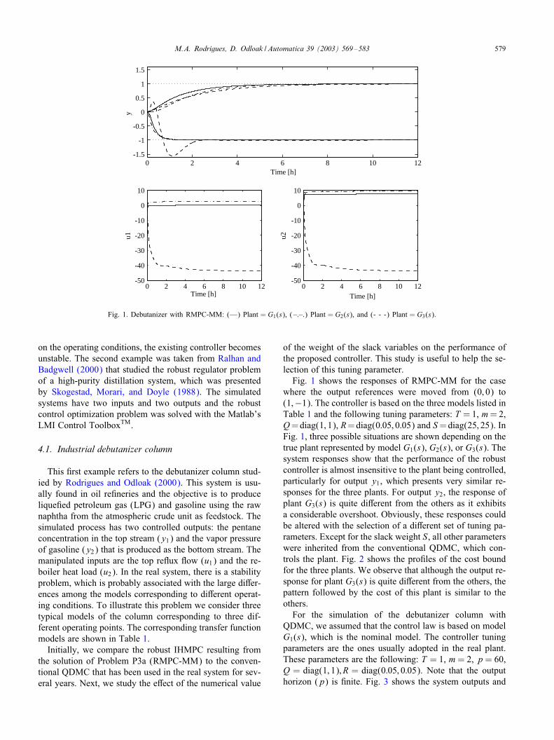
Fig. 1. Debutanizer with RMPC-MM: (—) Plant = G1(s), (–.–.) Plant = G2(s), and (- - -) Plant = G3(s).

on the operating conditions, the existing controller becomesunstable. The second example was taken from Ralhan andBadgwell (2000) that studied the robust regulator problemof a high-purity distillation system, which was presentedby Skogestad, Morari, and Doyle (1988). The simulatedsystems have two inputs and two outputs and the robustcontrol optimization problem was solved with the Matlab’sLMI Control ToolboxTM.

4.1. Industrial debutanizer column

This 2rst example refers to the debutanizer column stud-ied by Rodrigues and Odloak (2000). This system is usu-ally found in oil re2neries and the objective is to producelique2ed petroleum gas (LPG) and gasoline using the rawnaphtha from the atmospheric crude unit as feedstock. Thesimulated process has two controlled outputs: the pentaneconcentration in the top stream (y1) and the vapor pressureof gasoline (y2) that is produced as the bottom stream. Themanipulated inputs are the top reTux Tow (u1) and the re-boiler heat load (u2). In the real system, there is a stabilityproblem, which is probably associated with the large di9er-ences among the models corresponding to di9erent operat-ing conditions. To illustrate this problem we consider threetypical models of the column corresponding to three dif-ferent operating points. The corresponding transfer functionmodels are shown in Table 1.Initially, we compare the robust IHMPC resulting from

the solution of Problem P3a (RMPC-MM) to the conven-tional QDMC that has been used in the real system for sev-eral years. Next, we study the e9ect of the numerical value

of the weight of the slack variables on the performance ofthe proposed controller. This study is useful to help the se-lection of this tuning parameter.Fig. 1 shows the responses of RMPC-MM for the case

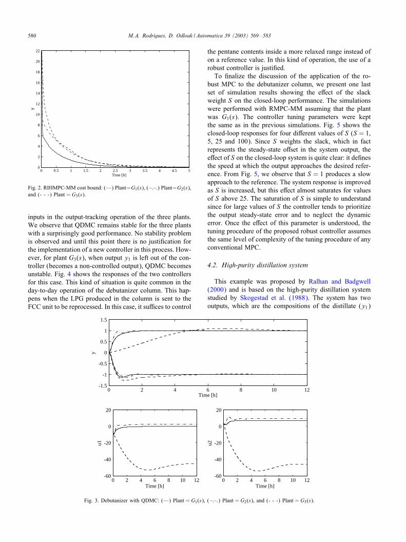
where the output references were moved from (0; 0) to(1;−1). The controller is based on the three models listed inTable 1 and the following tuning parameters: T =1, m=2,Q=diag(1; 1), R=diag(0:05; 0:05) and S=diag(25; 25). InFig. 1, three possible situations are shown depending on thetrue plant represented by model G1(s), G2(s), or G3(s). Thesystem responses show that the performance of the robustcontroller is almost insensitive to the plant being controlled,particularly for output y1, which presents very similar re-sponses for the three plants. For output y2, the response ofplant G3(s) is quite di9erent from the others as it exhibitsa considerable overshoot. Obviously, these responses couldbe altered with the selection of a di9erent set of tuning pa-rameters. Except for the slack weight S, all other parameterswere inherited from the conventional QDMC, which con-trols the plant. Fig. 2 shows the pro2les of the cost boundfor the three plants. We observe that although the output re-sponse for plant G3(s) is quite di9erent from the others, thepattern followed by the cost of this plant is similar to theothers.For the simulation of the debutanizer column with

QDMC, we assumed that the control law is based on modelG1(s), which is the nominal model. The controller tuningparameters are the ones usually adopted in the real plant.These parameters are the following: T = 1, m= 2, p= 60,Q = diag(1; 1); R = diag(0:05; 0:05). Note that the outputhorizon (p) is 2nite. Fig. 3 shows the system outputs and


0 0.5 1 1.5 2 2.5 3 3.5 4 4.5 50

2

4

6

8

10

12

14

16

18

20

22

γ

Time [h]

Fig. 2. RIHMPC-MM cost bound: (—) Plant=G1(s), (–.–.) Plant=G2(s),and (- - -) Plant = G3(s).

inputs in the output-tracking operation of the three plants.We observe that QDMC remains stable for the three plantswith a surprisingly good performance. No stability problemis observed and until this point there is no justi2cation forthe implementation of a new controller in this process. How-ever, for plant G3(s), when output y1 is left out of the con-troller (becomes a non-controlled output), QDMC becomesunstable. Fig. 4 shows the responses of the two controllersfor this case. This kind of situation is quite common in theday-to-day operation of the debutanizer column. This hap-pens when the LPG produced in the column is sent to theFCC unit to be reprocessed. In this case, it suLces to control

0 2 4 6 8 10 12-1.5

-1

-0.5

0

0.5

1

1.5

y

Time [h]

0 2 4 6 8 10 12-60

-40

-20

0

20

u1

Time [h]0 2 4 6 8 10 12

-60

-40

-20

0

20

u2

Time [h]

Fig. 3. Debutanizer with QDMC: (—) Plant = G1(s), (–.–.) Plant = G2(s), and (- - -) Plant = G3(s).

the pentane contents inside a more relaxed range instead ofon a reference value. In this kind of operation, the use of arobust controller is justi2ed.To 2nalize the discussion of the application of the ro-

bust MPC to the debutanizer column, we present one lastset of simulation results showing the e9ect of the slackweight S on the closed-loop performance. The simulationswere performed with RMPC-MM assuming that the plantwas G1(s). The controller tuning parameters were keptthe same as in the previous simulations. Fig. 5 shows theclosed-loop responses for four di9erent values of S (S = 1,5, 25 and 100). Since S weights the slack, which in factrepresents the steady-state o9set in the system output, thee9ect of S on the closed-loop system is quite clear: it de2nesthe speed at which the output approaches the desired refer-ence. From Fig. 5, we observe that S = 1 produces a slowapproach to the reference. The system response is improvedas S is increased, but this e9ect almost saturates for valuesof S above 25. The saturation of S is simple to understandsince for large values of S the controller tends to prioritizethe output steady-state error and to neglect the dynamicerror. Once the e9ect of this parameter is understood, thetuning procedure of the proposed robust controller assumesthe same level of complexity of the tuning procedure of anyconventional MPC.

4.2. High-purity distillation system

This example was proposed by Ralhan and Badgwell(2000) and is based on the high-purity distillation systemstudied by Skogestad et al. (1988). The system has twooutputs, which are the compositions of the distillate (y1)


0 2 4 6 8 10 12-15

-10

-5

0

y1

Time [h]0 2 4 6 8 10 12

-1

-0.8

-0.6

-0.4

-0.2

0

y2

Time [h]

0 2 4 6 8 10 120

200

400

600

800

1000

1200

u1

Time [h]0 2 4 6 8 10 12

0

200

400

600

800

1000

1200

u2Time [h]

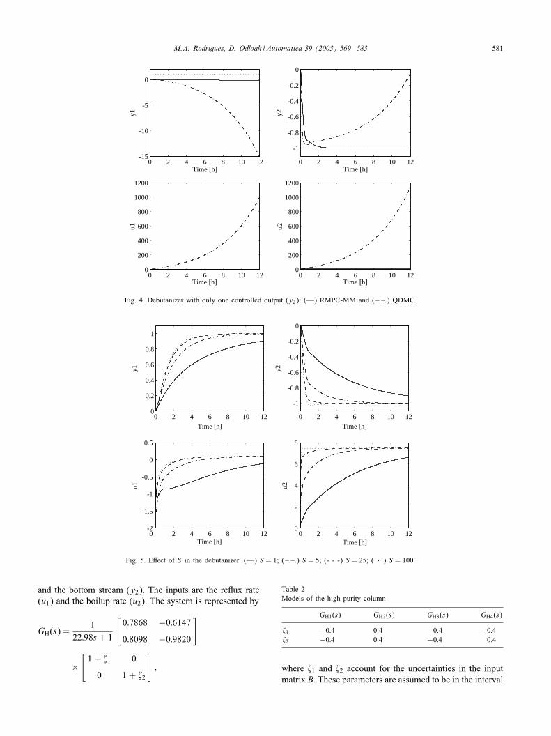
Fig. 4. Debutanizer with only one controlled output (y2): (—) RMPC-MM and (–.–.) QDMC.

0 2 4 6 8 10 120

0.2

0.4

0.6

0.8

1

y1

Time [h]0 2 4 6 8 10 12

-1

-0.8

-0.6

-0.4

-0.2

0

y2

Time [h]

0 2 4 6 8 10 12-2

-1.5

-1

-0.5

0

0.5

u1

Time [h]0 2 4 6 8 10 12

0

2

4

6

8

u2

Time [h]

Fig. 5. E9ect of S in the debutanizer. (—) S = 1; (–.–.) S = 5; (- - -) S = 25; (· · ·) S = 100.

and the bottom stream (y2). The inputs are the reTux rate(u1) and the boilup rate (u2). The system is represented by

GH(s) =1

22:98s+ 1

[0:7868 −0:6147

0:8098 −0:9820

]

×[1 + 01 0

0 1 + 02

];

Table 2Models of the high purity column

GH1(s) GH2(s) GH3(s) GH4(s)

01 −0:4 0.4 0.4 −0:402 −0:4 0.4 −0:4 0.4

where 01 and 02 account for the uncertainties in the inputmatrix B. These parameters are assumed to be in the interval


0 5 10 15 20

0

0.05

0.1

0.15

0.2

0.25

y1

k0 5 10 15 20

0

0.05

0.1

0.15

0.2

0.25

y2

k

0 5 10 15 20-1

-0.5

0

0.5

u1

k0 5 10 15 20

-0.5

0

0.5

1

u2k

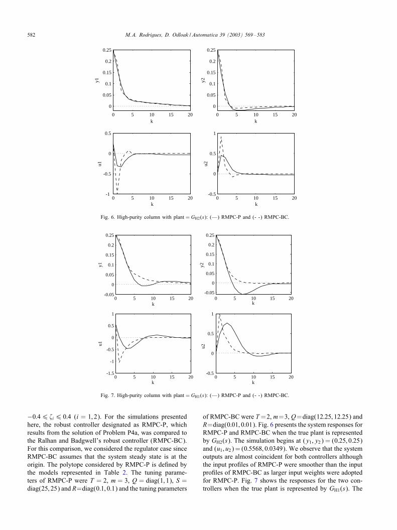
Fig. 6. High-purity column with plant = GH2(s): (—) RMPC-P and (- -) RMPC-BC.

0 5 10 15 20-0.05

0

0.05

0.1

0.15

0.2

0.25

y1

k0 5 10 15 20

-0.05

0

0.05

0.1

0.15

0.2

0.25

y2

k

0 5 10 15 20-1.5

-1

-0.5

0

0.5

1

u1

k0 5 10 15 20

-0.5

0

0.5

1

u2

k

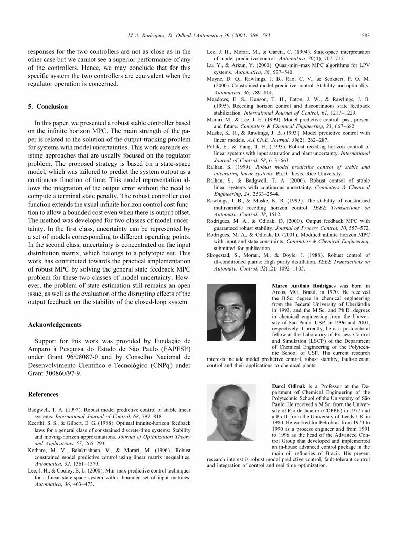
Fig. 7. High-purity column with plant = GH1(s): (—) RMPC-P and (- -) RMPC-BC.

−0:46 0i6 0:4 (i = 1; 2). For the simulations presentedhere, the robust controller designated as RMPC-P, whichresults from the solution of Problem P4a, was compared tothe Ralhan and Badgwell’s robust controller (RMPC-BC).For this comparison, we considered the regulator case sinceRMPC-BC assumes that the system steady state is at theorigin. The polytope considered by RMPC-P is de2ned bythe models represented in Table 2. The tuning parame-ters of RMPC-P were T = 2, m = 3, Q = diag(1; 1), S =diag(25; 25) and R=diag(0:1; 0:1) and the tuning parameters

of RMPC-BC were T=2, m=3, Q=diag(12:25; 12:25) andR=diag(0:01; 0:01). Fig. 6 presents the system responses forRMPC-P and RMPC-BC when the true plant is representedby GH2(s). The simulation begins at (y1; y2) = (0:25; 0:25)and (u1; u2)= (0:5568; 0:0349). We observe that the systemoutputs are almost coincident for both controllers althoughthe input pro2les of RMPC-P were smoother than the inputpro2les of RMPC-BC as larger input weights were adoptedfor RMPC-P. Fig. 7 shows the responses for the two con-trollers when the true plant is represented by GH1(s). The


responses for the two controllers are not as close as in theother case but we cannot see a superior performance of anyof the controllers. Hence, we may conclude that for thisspeci2c system the two controllers are equivalent when theregulator operation is concerned.

5. Conclusion

In this paper, we presented a robust stable controller basedon the in2nite horizon MPC. The main strength of the pa-per is related to the solution of the output-tracking problemfor systems with model uncertainties. This work extends ex-isting approaches that are usually focused on the regulatorproblem. The proposed strategy is based on a state-spacemodel, which was tailored to predict the system output as acontinuous function of time. This model representation al-lows the integration of the output error without the need tocompute a terminal state penalty. The robust controller costfunction extends the usual in2nite horizon control cost func-tion to allow a bounded cost even when there is output o9set.The method was developed for two classes of model uncer-tainty. In the 2rst class, uncertainty can be represented bya set of models corresponding to di9erent operating points.In the second class, uncertainty is concentrated on the inputdistribution matrix, which belongs to a polytopic set. Thiswork has contributed towards the practical implementationof robust MPC by solving the general state feedback MPCproblem for these two classes of model uncertainty. How-ever, the problem of state estimation still remains an openissue, as well as the evaluation of the disrupting e9ects of theoutput feedback on the stability of the closed-loop system.

Acknowledgements

Support for this work was provided by FundaVcao deAmparo Wa Pesquisa do Estado de Sao Paulo (FAPESP)under Grant 96/08087-0 and by Conselho Nacional deDesenvolvimento CientXY2co e TecnolXogico (CNPq) underGrant 300860/97-9.

References

Badgwell, T. A. (1997). Robust model predictive control of stable linearsystems. International Journal of Control, 68, 797–818.

Keerthi, S. S., & Gilbert, E. G. (1988). Optimal in2nite-horizon feedbacklaws for a general class of constrained discrete-time systems: Stabilityand moving-horizon approximations. Journal of Optimization Theoryand Applications, 57, 265–293.

Kothare, M. V., Balakrishnan, V., & Morari, M. (1996). Robustconstrained model predictive control using linear matrix inequalities.Automatica, 32, 1361–1379.

Lee, J. H., & Cooley, B. L. (2000). Min–max predictive control techniquesfor a linear state-space system with a bounded set of input matrices.Automatica, 36, 463–473.

Lee, J. H., Morari, M., & Garcia, C. (1994). State-space interpretationof model predictive control. Automatica, 30(4), 707–717.

Lu, Y., & Arkun, Y. (2000). Quasi-min–max MPC algorithms for LPVsystems. Automatica, 36, 527–540.

Mayne, D. Q., Rawlings, J. B., Rao, C. V., & Scokaert, P. O. M.(2000). Constrained model predictive control: Stability and optimality.Automatica, 36, 789–814.

Meadows, E. S., Henson, T. H., Eaton, J. W., & Rawlings, J. B.(1995). Receding horizon control and discontinuous state feedbackstabilization. International Journal of Control, 61, 1217–1229.

Morari, M., & Lee, J. H. (1999). Model predictive control: past, presentand future. Computers & Chemical Engineering, 23, 667–682.

Muske, K. R., & Rawlings, J. B. (1993). Model predictive control withlinear models. A.I.Ch.E. Journal, 39(2), 262–287.

Polak, E., & Yang, T. H. (1993). Robust receding horizon control oflinear systems with input saturation and plant uncertainty. InternationalJournal of Control, 58, 613–663.

Ralhan, S. (1999). Robust model predictive control of stable andintegrating linear systems. Ph.D. thesis. Rice University.

Ralhan, S., & Badgwell, T. A. (2000). Robust control of stablelinear systems with continuous uncertainty. Computers & ChemicalEngineering, 24, 2533–2544.

Rawlings, J. B., & Muske, K. R. (1993). The stability of constrainedmultivariable receding horizon control. IEEE Transactions onAutomatic Control, 38, 1512.

Rodrigues, M. A., & Odloak, D. (2000). Output feedback MPC withguaranteed robust stability. Journal of Process Control, 10, 557–572.

Rodrigues, M. A., & Odloak, D. (2001). Modi2ed in2nite horizon MPCwith input and state constraints. Computers & Chemical Engineering,submitted for publication.

Skogestad, S., Morari, M., & Doyle, J. (1988). Robust control ofill-conditioned plants: High purity distillation. IEEE Transactions onAutomatic Control, 32(12), 1092–1105.

Marco Antonio Rodrigues was born inArcos, MG, Brazil, in 1970. He receivedthe B.Sc. degree in chemical engineeringfrom the Federal University of Uberlandiain 1993, and the M.Sc. and Ph.D. degreesin chemical engineering from the Univer-sity of Sao Paulo, USP, in 1996 and 2001,respectively. Currently, he is a postdoctoralfellow at the Laboratory of Process Controland Simulation (LSCP) of the Departmentof Chemical Engineering of the Polytech-nic School of USP. His current research

interests include model predictive control, robust stability, fault-tolerantcontrol and their applications to chemical plants.

Darci Odloak is a Professor at the De-partment of Chemical Engineering of thePolytechnic School of the University of SaoPaulo. He received a M.Sc. from the Univer-sity of Rio de Janeiro (COPPE) in 1977 anda Ph.D. from the University of Leeds-UK in1980. He worked for Petrobras from 1973 to1990 as a process engineer and from 1991to 1996 as the head of the Advanced Con-trol Group that developed and implementedan in-house advanced control package in themain oil re2neries of Brazil. His present

research interest is robust model predictive control, fault-tolerant controland integration of control and real time optimization.

MPC for stable linear systems with model uncertainty

Documents