MPBEP_2011_04_Rpt_EcologicalImpactsoftheMPBonPineForestsoftheSouthernFoothillsAB

Ecological Impacts of the Mountain Pine Beetle on Pine Forests of the Southern Foothills, Alberta

A Case Study in Waterton Lakes National Park Jodi Axelson† Dr. René Alfaro‡ Dr. Brad Hawkes§

† University of Victoria, Department of Geography, Victoria BC. E-mail: [email protected] ‡ Canadian Forest Service, Pacific Forestry Centre, Victoria BC. E-mail: [email protected] § Canadian Forest Service, Pacific Forestry Centre, Victoria BC. E-mail: [email protected]

i

Table of Contents Introduction......................................................................................................................... 1

History of Project............................................................................................................ 4 Project Objectives ............................................................................................................... 4 Methods............................................................................................................................... 5

1981 Field Methods ........................................................................................................ 5 2002 Field Methods ........................................................................................................ 7

Overstorey................................................................................................................... 7 Understorey Regeneration .......................................................................................... 7 Downed Woody Debris............................................................................................... 8

2010 Field Methods ........................................................................................................ 8 Dendroecological Sampling........................................................................................ 8

Laboratory Methods........................................................................................................ 9 Data Analysis ................................................................................................................ 10

Data Storage.............................................................................................................. 10 Height estimation ...................................................................................................... 11 Data Analysis ............................................................................................................ 11 Dendroecological Analysis ....................................................................................... 11

Results............................................................................................................................... 13 Change in the Overstorey.............................................................................................. 13

Stand Density ............................................................................................................ 13 Stand volume ............................................................................................................ 16 Stand Basal Area....................................................................................................... 18 ................................................................................................................................... 20

Changes in Undestorey ................................................................................................. 20 Saplings..................................................................................................................... 20 Regeneration ............................................................................................................. 22

Coarse woody debris and fine fuels .............................................................................. 26 Dendroecology.............................................................................................................. 28

Cross-Dated Series.................................................................................................... 28 Cohort Ages .............................................................................................................. 28 Disturbance History .................................................................................................. 30 Integration of Tree-ring Chronologies ...................................................................... 35

Discussion......................................................................................................................... 38 Disturbance history ....................................................................................................... 38 Overstorey mortality and stocking................................................................................ 39 Canopy response ........................................................................................................... 39 Regeneration ................................................................................................................. 40 Fuels.............................................................................................................................. 41

Conclusion ........................................................................................................................ 42 Acknowledgements........................................................................................................... 43 References......................................................................................................................... 43 Appendix 1........................................................................................................................ 48 Appendix 2........................................................................................................................ 53 Appendix 3........................................................................................................................ 55

1

Introduction Natural disturbances are one of the principal mechanisms that shape the composition and structure of forest ecosystems (White 1979). Understanding the characteristics of the disturbance regime is a starting point to quantify their effects on ecosystem services and forest productivity (Oliver 1981, Agee 1993). As a natural agent of disturbance, the mountain pine beetle (Dendroctonus ponderosae Hopkins; MPB) is the most significant forest insect affecting lodgepole pine forests in western North America (Furniss and Carolin 1977). Almost all pine species in western North America are suitable hosts for MPB, however lodgepole pine (Pinus contorta var. latifolia Engelm.) is one of the most susceptible and most widely distributed species in North America, and where the economic impacts are the heaviest. MPB outbreaks have occurred over entire landscapes, and the duration and severity of an outbreak is dependent on factors such as: the size of the beetle population; degree of susceptible stands distributed over the landscape, and stand characteristics such as species composition, age, diameter and density; and climate (Safranyik 2004). Natural resource managers increasingly rely on the natural range of variability (NRV) to develop plans that guide management within the range of ecological conditions appropriate for the area (Landres et al. 1999). Understanding the NRV of biotic disturbances on and across the landscape requires a sound understanding of past disturbances. This is crucial for predicting how ecosystems will change, even in response to novel processes. In Alberta, sustainable forest management requires detailed understanding of stand dynamics and legacies resulting from MPB outbreaks. This knowledge is crucial to managing second-growth forests in a manner that approximates natural disturbance regimes, while also reducing future risk of economic losses from MPB attacks. Increasingly, this type of ecological information is critically important, especially as climate change is likely to change the spatial and temporal characteristics, and the severity of these disturbances (Volney and Fleming 2000, Kurz et al. 2008). Historical ecology provides information on NRV through long-term sequence of measurements that describes past conditions and disturbance regimes, such as changes in ecosystem structure, disturbance frequencies and other dynamic processes (Swetnam et al. 1999). Dendroecology, the study of tree-rings in an ecosystem context, has been used to evaluate biotic (e.g., insect outbreaks) and abiotic (e.g. fire) forest disturbances. Tree-rings can tell a story of canopy disturbance(s) and have been useful in identifying past insect outbreaks beyond the 20th century, extending limited documented records (Swetnam et al. 1999). For example, bark beetles have eruptive populations that can result in 60 to 90 percent mortality of mature hosts during an outbreak (Raffa et al. 2008), and are therefore considered a stand releasing disturbance (Veblen et al. 1991a;b, Berg et al. 2006). MPB outbreaks are reconstructed beyond the observed record by quantifying release signals in rings from trees that survive outbreaks. When insects kill the host trees in a stand and the surviving host or non-host trees sustain an increase in radial growth due to reduced competition in the stand. Reconstructions of bark beetle outbreaks have been done for MPB in British Columbia (e.g., Heath and Alfaro 1990, Alfaro et. al. 2004, Campbell et al. 2007, Axelson et al. 2009; 2010) and in the Front Ranges of the Rocky

2

Mountains in the United States (e.g., Romme et al. 1986, Sibold et al. 2007). Dendroecological studies indicate that there have been four to five significant MPB outbreaks in British Columbia during the last century, with an average duration of 10 years (Alfaro et al. 2004, Taylor et al. 2006). In the northern Rocky Mountains of the United States MPB outbreaks occur every 20 to 40 years and typically last 6 years (Cole and Amman 1980). Another effect of MPB on stand dynamics is the establishment of regeneration in the stand as more light and space are available for seed germination. Depending on the species composition of the overstorey and understorey, MPB outbreaks can accelerate sucessional dynamics towards more shade-tolerant species (Roe and Amman 1970, Heath and Alfaro 1990, Axelson et al. 2009), although if climate and edaphic conditions are suitable, lodgepole pine can regenerate under its own canopy resulting in a self-perpetuating system (Agee 1993). While large portions of the mature canopy can be killed during a MPB outbreak, numerous studies have demonstrated ecosystem resilience to such disturbances. In the central interior of British Columbia Heath and Alfaro (1990) found that the radial growth rate of residual Douglas-fir was enhanced for 14 years after MPB attack, suggesting the possibility that stand volume lost by pine might be compensated for by increased fir growth by the time harvest rotation was reached. In the Yellowstone region of the Rocky Mountains Romme et al. (1986) found that lodgepole pine stands were highly resilient to MPB outbreaks; the effects of the MPB on primary productivity were compensated for, or exceeded by, growth releases in previously suppressed trees, and there was a greater equitability of biomass and energy flow among various components of the ecosystem through increased structural complexity (Romme et al. 1986). Sibold et al. (2007) examined the effects of secondary disturbances on fire initiated even-aged stands of lodgepole pine in the southern Rocky Mountains in the United States. In these stands large portions of the canopy were killed by MPB during an outbreak, which initially decreased tree density, but later triggered large amounts of new tree establishment. The density of the lodgepole pine or subalpine fir establishment following MPB outbreaks was related to the severity of the disturbance and the time since the last stand initiating fire. They found that in younger stands high-severity disturbance resulted in dense lodgepole pine establishment, while in older stands high-severity disturbances resulted in mixed lodgepole pine and subalpine fir establishment, while moderate-severity disturbances favoured subalpine fir establishment (Sibold et al. 2007). Mountain pine beetle outbreaks are a patchy disturbance when considered over the landscape scale. In many pine dominated landscapes it is likely that a shift in the predominant disturbance type from severe stand replacing fires to MPB outbreaks would result in considerable heterogeneity of stand age structure, tree density and species composition (Sibold et al. 2007). This has been found at relatively fine scales in the southern interior (Axelson et al. 2009) and central interior (Hawkes et al. 2004a, Axelson et al. 2010) of British Columbia. In the southern interior stand replacing fires initiated even-aged stands of lodgepole pine, and repeated MPB outbreaks resulted in waves of canopy mortality, stand-wide growth releases and establishment of primarily shade tolerant species such as Douglas-fir (Axelson et al. 2009). In the central interior, on the other hand, mature lodgepole pine stands resulted from mixed severity fires, creating

3

uneven-aged stand structure. The dominant disturbance type has shifted from fire (due to suppression activities) to MPB outbreaks, and stands are periodically thinned from above resulting in canopy mortality and stand-wide growth releases in survivors. Regeneration in these stands was primarily lodgepole pine; therefore outbreaks are not hastening succession to shade tolerant species (Hawkes et al. 2004a, Axelson et al. 2010). This scenario also exists in central Oregon, where lodgepole pine forests are uneven-aged, and experience distinct episodic pulses of mainly lodgepole pine regeneration that are strongly correlated to MPB outbreaks and fire (Stuart el al. 1989, Mitchell and Priseler 1998). As in the southern Rockies (Sibold et al. 2007) the magnitude of the regeneration was a function of the disturbance intensity. While these studies demonstrated successful pine and non-pine regeneration after MPB outbreaks this is highly ecosystem dependent. For example, Astrup et al. (2008) demonstrated that recruitment of new seedlings after MPB was substantially lower than observed after wildfires in the Sub-boreal Spruce (SBS) biogeoclimatic (BEC) zone in northern British Columbia. In this region substrate availability and suitability was an important factor in seedling establishment; the forest floor continued to be dominated by moss years after the MPB outbreak and thus overall recruitment of regeneration was low. Mortality in lodgepole pine stands by MPB could influence fire behaviour, as tree mortality changes the spatial distribution of fuels in the forest. Information that is lacking is the link between the mortality rate of trees in lodgepole pine forests under attack by MPB and the subsequent fuel loading of the stand. The length of time that dead trees remain standing and the rate at which they decay once they have fallen to the ground is highly variable and specific to the site (Shore et al. 2006). Mitchell and Preisler (1998) found that in un-thinned lodgepole pine stands in southern Oregon, MPB-killed trees began to fall to the forest floor after 5 years; 50 percent of trees fell within 9 years, and 90 percent fell by 14 years post-attack. Turner et al. (1999) found that high severity MPB attacks (defined by >50 percent of trees killed) increased crown fire probability, but intermediate or light levels of MPB severity reduced crown fire probability during the wildfires of 1988 in Yellowstone National Park. Although a hazard rating model for MPB in lodgepole pine forests exists (Shore and Safranyik 1992), an understanding of how fuels are altered by MPB is necessary in order to use fire behaviour prediction models in conjunction with growth and yield (G&Y) models. These linkages are critical to understand landscape level MPB impacts. On the east slopes of the Rocky Mountains, lodgepole pine is found in nearly all forested regions (Alberta Environmental Protection 1994) making up 50 percent of forests in the Upper Foothills and 20 percent of forests in the Lower Foothills natural sub-regions (Alberta Sustainable Resource Development 2007). Hopping and Mathers (1945) documented a MPB outbreak on the east slopes north of Banff in the late 1940s. Alfaro et al. (2006) detected widespread and synchronous growth releases in the 1930s and 1940s and again in the late 1970s and 1980s across the British Columbia interior and south-western regions of Alberta in response to MPB outbreaks. Although MPB outbreaks generally were not that well documented in the 1930s in Alberta, Richmond (1983) documented large outbreaks in BC in the 1920s and 1930s. Alfaro et al. (2006) found significant stand-wide releases in lodgepole pine and non-host species (e.g., Douglas-fir and spruce) in the south-western portion of Alberta, indicative of widespread

4

canopy thinning by beetle. Forest Insect and Disease Surveys (FIDS) records document an active MPB outbreak in south-western Alberta from 1977 to 1986 (Brandt and Amirault 1994), which peaked in 1981. Cumulatively, this outbreak resulted in over 1 million cubic meters (m3) of lodgepole pine mortality from 1977 to 1987 (Brandt and Amirault 1994). The recent (circa 2008) population expansion and spread of MPB into central and northern latitudes of the east slopes puts extensive areas of lodgepole pine ecosystems at risk (Alberta Sustainable Resource Development 2007), potentially threatening more than two million hectares of pine forests with an estimated commercial value of $23 billion (Alberta Sustainable Resource Development 2005). While a number of studies have been conducted in British Columbia to evaluate stand dynamics and G&Y of lodgepole pine stands following MPB outbreaks, there is a deficiency of such information for Alberta.

History of Project In Waterton Lakes National Park (WLNP) MPB was first detected in 1977. In 1980 the parks staff and FIDS rangers from the CFS, under the leadership of Dr. Ben Moody of Northern Forestry Centre, established 25 permanent monitoring plots in the park. In 2002, under the leadership of Dr. Brad Hawkes of the Pacific Forestry Centre, funding was secured to re-measure plots in WLNP. This re-measurement provided an opportunity to examine stand dynamics and recovery in response to the 1980s MPB epidemic in south-western Alberta. In addition, the 2002 re-measurement provided the opportunity to collect and data on and evaluates regeneration, coarse woody debris and fuel loads (Hawkes et al. 2004b). In 2008-09, under the leadership of Dr. René Alfaro from the Pacific Forestry Centre, dendroecological research was conducted under the Foothills Growth and Yield project “Monitoring and Decision Support for Forest Management in a Mountain Pine Beetle Environment” (Alfaro et al. 2009). Dendroecological analysis provided important information on stand processes such as initiation, canopy disturbances, mortality and regeneration from 14 permanent samples plots of the G&Y Association partners between Nordegg and Grand Prairie. In 2010 a proposal to re-measure the permanent plots in WLNP was funded jointly by the Foothills Research Institute MPB Ecology Program and the Canadian Forest Service MPB Initiative Fund. This research begins to fill key regional gaps in the southern Rocky Mountains, although gaps remain from the Crowsnest area (to the south) to Rocky Mountain House (to the north) along the east slopes.

Project Objectives This project takes advantage of long-term permanent monitoring plots in WLNP that have experienced MPB outbreaks. In this unmanaged environment the ecological processes related to MPB outbreaks in south-western Alberta can be evaluated in the context of previous measurement data, with the addition of dendroecological techniques. This project provides much needed information to guide resource managers and decision makers on ecological impacts and future forest productivity in a MPB environment in Alberta.

5

Specifically the project objectives include: • Develop ecological baselines of biotic disturbances in Waterton Lakes National

Park using a dendroecological approach. This will include reconstructing past MPB outbreaks and the mortality and regeneration dynamics post-disturbance;

• Examine how biotic disturbances affect future forest structure. Forest structure (e.g., diameter distributions, species composition, age class distributions) have direct implications for the expected ecosystem services in the long-term;

• Integrate dendroecological data collected in this project with previous surveys in the central and northern Rocky Mountains to provide a comprehensive picture of disturbance regimes ands stand dynamics for the east slopes.

The current project provides a unique time series of forest change through time, and the timing of ecological processes such as stand initiation, canopy disturbances, overstorey mortality and regeneration. The project provides information on changes to coarse woody debris and fuel loads in stands impacted by MPB. Knowledge of post-MPB attack stand dynamics will help forest managers make decisions to meet their long-term strategic plans, and will assist G&Y simulation models to forecast future forest conditions under a variety of scenarios of varying disturbance regimes or management.

Methods Copies of the original data forms were available from WLNP, which allowed for the re-location and re-measurement of the original permanent sample plots, and provided some guidance in documenting the original methods used. The following describes, based on the reports and data available, the methods that were used in sampling from 1981 to 1983.

1981 Field Methods Five stands were selected throughout low elevation regions of the park, although specific criteria for stand selection were not documented. Exact locations of plots are listed in Appendix 1. The following stands were chosen for establishment of permanent plots (Fig. 1): Stand 1: Crandell (CR) Located on the south side of the Red Rock Parkway near the Crandell Mountain Campground. Stand 2: Fire Road (FR) Located on the Chief Mountain Highway opposite of the Bellevue Look-out pull- out. Stand 3: Bellevue Look-out (BV) Located on the Chief Mountain Highway at the Bellevue Look-out pull-out on south-west side of highway.

6

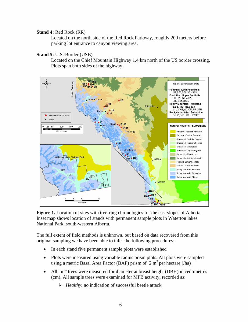
Stand 4: Red Rock (RR) Located on the north side of the Red Rock Parkway, roughly 200 meters before parking lot entrance to canyon viewing area. Stand 5: U.S. Border (USB) Located on the Chief Mountain Highway 1.4 km north of the US border crossing. Plots span both sides of the highway.

Figure 1. Location of sites with tree-ring chronologies for the east slopes of Alberta. Inset map shows location of stands with permanent sample plots in Waterton lakes National Park, south-western Alberta. The full extent of field methods is unknown, but based on data recovered from this original sampling we have been able to infer the following procedures:

• In each stand five permanent sample plots were established

• Plots were measured using variable radius prism plots. All plots were sampled using a metric Basal Area Factor (BAF) prism of 2 m2 per hectare (/ha)

• All “in” trees were measured for diameter at breast height (DBH) in centimetres (cm). All sample trees were examined for MPB activity, recorded as:

Healthy: no indication of successful beetle attack

7

Current: attacked by MPB, with pitch tubes present or live beetles under the bark

Red: recently MPB-killed tree with red foliage

Grey: 2+ years since MPB kill

Partial: evidence of MPB attack, but tree is healthy still

• Some trees (unequal numbers per plot) were measured for total height in metres (m).

Beetle activity was re-assessed for all sample trees in 1982 and 1983, but no further measurements were taken.

2002 Field Methods Plots were re-measured in October 2002. Within each stand, the center of each plot was relocated and an orange-painted aluminum stake was hammered into the ground as a permanent marker to replace the original wooden stakes. The location of each stand was recorded using Global Positioning Systems (GPS). In addition to this, a detailed map was drawn with driving directions, stand location, and the direction and distance between plots. For each forest component the following measurements were collected:

Overstorey

• All trees from the initial study were relocated and identified in each plot. Trees that had fallen since the previous assessment were noted. Metal tags were hammered into all standing trees (dead or alive) to replace original tags. DBH was recorded for all standing trees.

• Any new trees that had grown “in” to the plot (BAF 2m2/ha) were labeled with metal tags, and noted as new on field form. A DBH of 7.0 cm was the lower limit was set for tree sampling. DBH measured.

• Dead trees were examined to determine the cause of death. If beetle galleries were present, they were examined to determine whether it was MPB or Ips species that had killed the tree. The height of all snags was estimated and each snag was assigned to a decay class using criteria contained in Wildlife Tree Committee of BC (2001).

• For increment coring and height measurements, two lodgepole pine trees per plot were randomly chosen (the lowest and highest tree number in each prism plot) and measured for total height and height to the bottom of the live crown. These same trees were increment cored. If other tree species were present in the plots, they were also measured for total height and height to live crown.

• Increment cores were labeled with new tag numbers and stored in plastic straws.

Understorey Regeneration

8

No understorey or regeneration data was collected in the 1981 measurement. Using the new aluminum stake for plot centre fixed area plots were established to measure saplings and seedlings.

• Saplings greater than 1.5 m in height and less than 7.0 cm DBH were counted in a 5.64 m or 7.98 m radius circle. The radius of the plot was chosen to capture a minimum of 6 saplings in the plot. Saplings were tallied by species in two DBH classes: A = 0-3.9 cm and B = 4.0-7.0 cm.

• Seedlings less than or equal to 1.5 m in height were counted in a 3.1 m radius circle. Seedlings were tallied by species and height class (0-0.10 m, 0.10-0.50 m, 0.50-1.0 m, 1.0-1.5 m).

Downed Woody Debris No measurements of coarse woody debris (CWD) or fine fuels were collected in 1981. In 2002 in each plot, CWD (> 7 cm diameter) and fine fuels (< 7 cm diameter) were measured along a 30 m transect on a random compass bearing from plot center.

• A 30m tape was laid out on the ground, and for coarse woody debris, the diameter and species of each piece intersected by the transect tape was recorded. Each piece was assigned to one of five classes of decomposition. A nail was hammered into all pieces of CWD that intersected the line and were marked with fluorescent paint.

• Fine fuels were tallied along the first 25m of the transect line using the method by Trowbridge et al. (1986).

• The end of the transect line was marked with an aluminum stake.

2010 Field Methods Plots were re-measured in September 2010. The center of each plot was relocated and overstorey, understorey and downed woody debris measurements were collected following the 2002 methodology (see above). For only the Red Rock stand, depth of burn pins were placed 1m perpendicular on each side of the 5m fuel transect points up to and including 25m for a total of 10 depth of burn pins per transect. This was done to ensure forest floor consumption would be documented in a proposed Parks Canada prescribed burn which may burn over this stand in the spring of 2012. In addition to re-measurement, dendroecological cookie samples were collected for CWD.

Dendroecological Sampling Each stand was intensively sampled in order to reconstruct the temporal dynamics of stand initiation, stand structure and cohort ages, canopy disturbances, overstorey mortality and establishment of regeneration. Data from this work indicates how stands progressed towards their present day composition and structures. The following sampling was performed (Fig. 2):

• Collected a sub-sample of increment cores at breast height from live “in” plot trees and large trees that were outside of variable radius plots. Increment cores

9

were collected for lodgepole pine and other non-host species that occupied dominant or co-dominant status in the canopy (e.g., subalpine fir, Douglas fir and white spruce). Increment cores were labelled and stored in plastic straws.

• Basal cookies were collected from understorey trees (DBH < 7.0 cm) outside of the permanent sample plots. Trees were selected in an attempt to capture the range of understorey tree sizes reflected within the permanent sample plots. Tree height and diameter at ground height (DGH, cm) was measured for each tree before sampling. Around 5 trees per plot area for a total of 20 samples per stand were cut down above the root collar. Samples were labelled with a permanent marker and stored in plastic bags grouped by stand.

• Cross-sectional discs were collected from around 10 samples of coarse woody debris (> 7 cm DBH) outside of the plots and away from the CWD sampling transects. The largest downed trees were sampled, and samples were cut at the tree base. Discs were labelled on both sides of the sample with permanent marker and stored together by stand. One of the limitations of assessing past stand disturbances using CWD is that much of the oldest downed debris has undergone some degree of decay and cannot be dated using the methods of dendrochronology, thus the number of datable samples decreases farther back in time.

Figure 2. Collecting dendroecological samples: a) increment coring around breast height; b) destructive sample of understorey tree; c) collecting disc from CWD.

Laboratory Methods All dendroecological samples were processed using standard dendrochronology methods (Stokes and Smiley 1968). All samples were air dried and increment cores were glued to slotted wooded mounts. Coarse woody debris samples that had more advanced decay were glued to plywood to stabilize the sample for sanding. All samples were sanded using progressively finer sandpaper (120 to 600 grit) in order to precisely identify annual ring boundaries. All samples were then scanned and measured using WinDendroTM (v.2008g Regent Instruments Inc. 2009), with a measurement precision of 0.01 mm (Fig.

10

3). All the measured ring-width series were plotted and the patterns of wide and narrow rings were cross-dated among trees to identify possible errors in measurement due to false or locally absent rings. The program COFECHA (Holmes 1983) was used to detect errors and verify cross-dating. Dated live tree-ring series from each stand were used to cross-date dead trees. Cross-dated cores from 2002 were added to the 2010 cross-dated files.

Figure 3. Example of a live lodgepole pine increment cored being measured with the WinDendro system.

Data Analysis

Data Storage Data collected in 1981-1983 had been stored on paper at the Waterton Lakes National Park headquarters. These data sheets were photocopied from the originals making some entries unclear. These data and that collected in 2002 were entered into a Microsoft Excel spreadsheet. Data collected in 2010 was added to the Excel spreadsheet. Some important assumptions were made when finalizing the data within the master spreadsheet for all of the measurement years (1981-1983, 2002 and 2010):

• Health status codes (see 1981 Field Methods) of overstorey trees measured in 1981 were changed to the 1982 coding. This was done because the poor quality of the photocopied data forms made a number of the 1981 status codes illegible.

11

• There were five missing DBH values for overstorey trees in 1981. To estimate DBH for these trees a stand average by species was computed for the 2002 and 1981 data. This gave an average difference between DBH of the two measurement years. This value was subtracted from the 2002 measured DBH to obtain an estimated DBH for trees missing this value in 1981.

• In 2010 field notes did not indicate for all dead trees whether the tree was standing or down. As all standing dead trees had their DBH measured, we assumed that any dead tree that did not have a DBH measured was down.

Height estimation As mentioned in the field methods height data was collected at random from an uneven number of trees per plot in 1981, and only from trees that were cored in 2002. Height data was not collected in 2010. Missing height data was estimated for all trees for all measurement years. This was done by first sorting the master spreadsheet by: measurement year, species, and live trees. The list was then sorted again by those trees with a height measured in the field. If a tree had its height measured in 1981 and 2002 the 2002 height value was used. In the program StatisticaTM scatterplots of height (m) versus DBH (cm) were plotted with a logarithmic curve fitted. Regression equations were computed for each species, along with the r-value, and p-value to assess the goodness of fit and confidence of each equation. Height equations were applied to trees with no height data. Scatterplots and height estimation equations are presented in Appendix 1.

Data Analysis Data summaries for all measurement years were computed using SAS Analytics. For each measurement year tree density in stems per hectare (sph), volume per hectare (m3/ha) and basal area per hectare (m2/ha) were computed for live and dead trees by species on a plot and stand basis. All calculations were based on equations from Forestry Handbook for British Columbia (University of British Columbia Forestry Undergraduate Society 2005). Equations are listed in Appendix 1. For fuels data the program CWDFuel.exe (Ember Research Services 1997) was used to estimate the mass and volume of fine and coarse fuels in each stand.

Dendroecological Analysis The computer program ARSTAN (Cook and Holmes 1986, version ars_41) was used to produce a mean standardized ring-width chronology for each species. A negative exponential curve was used to standardize tree-ring series, which removes the early biological growth trend in each tree ring series. In addition to removing biological growth trends standardization transforms non-stationary ring-widths into a new series of stationary, relative tree-ring indices that have a defined mean of 1.0 and a relatively constant variance (Cook et al. 1990). All chronologies were fitted with a 15-year spline with a 50% frequency cut-off to highlight lower frequency variability within the time series.

12

The tree-ring program JOLTS (Holmes 1999, University of Arizona, unpublished) was used to detect growth releases in individual trees, by computing a ratio of the forward and backward 10-year running means of ring-widths for each year. If this ratio exceeded 1.25 (i.e., a 25% increase in radial growth) for a given year, we counted a release for that year. Running means have been found to produce results that agree well with documented canopy disturbances (Rubino and McCarthy 2004), and the 10-year window has been found to sufficiently smooth ring-width variability due to short-term climatic variation (Berg et al. 2006). The ratio of 1.25 has been used in previous studies to document growth releases and effectively identifies periods of canopy thinning due to mountain pine beetle outbreaks (Alfaro et al. 2004; Taylor et al. 2006; Campbell et al. 2007; Axelson et al. 2009; 2010). In addition to the growth release factor, 20 percent of the samples had to record the release to be considered a stand-wide disturbance. Tree-ring data were compiled to create comprehensive graphs that show stand initiation (based on inner most ring date of CWD samples and increment cores), canopy releases (based on JOLTS runs), stand mortality (based on outer-most ring date of CWD), and regeneration establishment episodes (based on pith date of destructively sampled advance regeneration). Standardized tree-ring chronologies collected in this study were integrated with those collected in the 2008-09 in the northern Foothills (Nordegg to Grande Prairie) (Alfaro et al. 2009), and those collected around Banff and Jasper in previous studies (Alfaro et al. 2004). All chronologies were fitted with a 15-year spline with a 50% frequency cut-off to highlight lower frequency variability within the time series. Trees in closed canopy forests usually sustain more non-climatic variability in growing conditions, both spatially and temporally, than trees in open canopy situations, and as a result the variation of the annual growth increment has a proportionately weaker climatic component (Peters et al. 1981). We employed Factor Analysis (FA) (Dunteman 1989) as a data reduction technique to identify and extract common patterns of growth variability across all of the east slopes lodgepole pine chronologies. This technique uncovers the major modes of variability in the data, and has been used to enhance our understanding of the growth patterns across the landscape (Fritts 1976). Varimax rotation was conducted on factors (herein, factor chronologies (FCs), sensu Peterson and Peterson 2001). Varimax rotation simplifies the interpretation of each original variable, which tends to be associated with one, or a small number of factors, and also maximizes the variance of the factor loadings (Kaiser 1958). Retention of factors was based on the Kaiser criterion where eigenvalues are equal to or greater than 1.0 (Kaiser 1960). Coefficients of variation (r2 > 0.70) were used to describe the association between the original tree-ring chronologies and the retained FCs. These analyses provides some insight on variations in tree-ring variability along the east slopes, and whether grouping would occur amongst southern tree-ring chronologies (with known MPB outbreaks) with chronologies to the north, which are assumed never to have MPB activity before.

13

Results In all of the tables and figures presented throughout this section tree species are abbreviated using tree species codes from the Field Manual for Describing Terrestrial Ecosystems (British Columbia Ministry of Forests and Range 2010):

• Bl: subalpine fir (Abies lasiocarpa) • Df: Douglas-fir (Pseudotsuga menziesii) • Pl: lodgepole pine (Pinus contorta) • Sw : white spruce (Picea glauca) • Acb: balsam poplar (Populus balsamifera) • At: trembling aspen (P. tremuloides) • Wa: willow (Salix spp.)

Lodgepole pine is the most common tree species in Waterton Lakes National Park. Seventy percent of the lodgepole pine-dominated stands at lower elevations in WLNP have a stand replacement fire regime with a fire return interval of 98 years (Barrett 1996). Thirty percent of the stands have a mixed severity fire regime with a fire return interval from 36-55 years (dry and moist sites, respectively) but these stands usually occurred on a burn margin of a nearby stand replacement fire (Barrett 1996). Most of the lower Waterton valley lodgepole pine stands date from fires in the mid to late 1800s as a single seral component. Lodgepole pine stands had matured sufficiently by the 1970s to be susceptible to MPB when the outbreak started in the late 1970s.

Change in the Overstorey

Stand Density The degree of tree mortality averaged for lodgepole pine in each stand is quite variable (Table 1). In 1981, up to 93 percent of pine were dead in stand 4 (Red Rock) and as little as 10 percent were dead in stand 1 (Crandell) (Table 1). Stands 2 (Fire Road), 3 (Bellevue Look-out) and 5 (U.S. Border) had more intermediate mortality levels in 1981 at 55, 32 and 29 percent respectively (Table 1). In stand 4, which had the greatest overall mortality for all measurement years, the total live sph ranged between 50 trees/ha to around 30 sph from 1981 to 2010. Interestingly, this is the only stand where tree density appears to increase by 2002, though only to 61 sph (Table 1). Tree density was split into live and dead categories and further subdivided by species (Table 2). In 1981, lodgepole pine was the dominant species making up live and dead stocking (Table 2). For example, stand 4 had a highest overall mortality (Table 1), which occurs almost exclusively in the pine cohort (94 percent) (Table 2). After 1981, species diversity increases across all stands between the 2002 and 2010 measurement years (Table 2, Fig. 4).

14

TABLE 1. Lodgepole pine density and percentages of live and dead standing pine. Stand

No. 1981 (sph)

Pl - % Live (% Dead)

2002 (sph)


2010 (sph)


1 1393 90 (10) 1203 72 (28) 1029 84 (16) 2 1180 45 (55) 727 39 (61) 361 76 (24) 3 1523 68 (32) 765 60 (40) 482 67 (33) 4 724 7 (93) 174 35 (65) 78 49 (51) 5 1163 71 (29) 739 65 (35) 487 80 (20)

Average 1197 56 (44) 721 54 (46) 487 71 (29) TABLE 2. Live and dead trees per hectare for each stand by species.

LIVE Stems/hectare

DEAD Stems/hectare Stand

No. Spp 1981 2002 2010 1981 2002 2010

1 Bl - 84 54 - - - Df - 103 75 - - - Pl 1248 865 865 145 338 164 Sw 38 219 219 - - - Acb - - - - - - At - - - - - - 2 Bl - 10 8 - - - Df 146 161 148 - - 9 Pl 533 281 274 648 446 86 Sw - 29 27 - - - Acb - - - - - - At 20 49 43 - - - 3 Bl - 16 153 - - - Df - - - - - - Pl 1034 458 324 489 307 157 Sw - - - - - - Acb - - - - - - At - - - - - - 4 Bl 103 98 63 - - 15 Df - - - - - - Pl 50 61 38 674 113 40 Sw 17 89 65 43 16 - Acb 8 9 8 - - - At - - - 67 72 5 Bl 24 18 17 - - - Df - 3 5 - - - Pl 828 479 391 335 260 96 Sw 146 161 126 18 7 22 Acb 79 194 136 - 31 54 At 23 16 - - 14 10

15

In 1981, live tree density was predominately lodgepole pine (e.g., stand 1 and 3), but by 2002 and 2010 had new species arriving (e.g., subalpine fir, Douglas-fir), or increased densities of non-pine species (e.g., white spruce). For example, stand 3 (Bellevue Look-out) goes from a pure stand of lodgepole pine in 1981, to having 47 percent of its live tree density made up of subalpine fir by 2010 (Fig. 4). Stands 2, 4 and 5 were initially mixed species stands in 1981 and have since become more mixed between 2002 and 2010. For example, stand 2 had a consistent cohort of Douglas-fir (between 25 to 35 percent), and stand 5 contained the highest amount of hardwoods such as balsam poplar and aspen (Fig. 4). Stand 4 has the lowest live tree density of any stand (< 400 sph), and is also one of the most mixed species stands, having substantial components of both subalpine fir and white spruce in all measurement years (Fig. 4).

Figure 4. Live tree density for each stand by species.

16

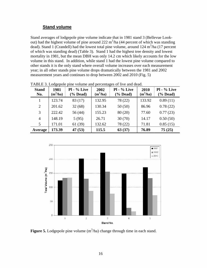
Stand volume Stand averages of lodgepole pine volume indicate that in 1981 stand 3 (Bellevue Look-out) had the highest volume of pine around 222 m3/ha (44 percent of which was standing dead). Stand 1 (Crandell) had the lowest total pine volume, around 124 m3/ha (17 percent of which was standing dead) (Table 3). Stand 1 had the highest tree density and lowest mortality in 1981, but the mean DBH was only 14.2 cm which likely accounts for the low volume in this stand. In addition, while stand 1 had the lowest pine volume compared to other stands it is the only stand where overall volume increases over each measurement year; in all other stands pine volume drops dramatically between the 1981 and 2002 measurement years and continues to drop between 2002 and 2010 (Fig. 5) TABLE 3. Lodgepole pine volume and percentages of live and dead.

Stand No.

1981 (m3/ha)


2002 (m3/ha)


2010 (m3/ha)


1 123.74 83 (17) 132.95 78 (22) 133.92 0.89 (11) 2 201.62 32 (68) 130.34 50 (50) 86.96 0.78 (22) 3 222.42 56 (44) 155.23 80 (20) 77.60 0.77 (23) 4 148.19 5 (95) 26.71 30 (70) 14.17 0.50 (50) 5 171.01 61 (39) 132.62 78 (22) 71.81 0.85 (15)

Average 173.39 47 (53) 115.5 63 (37) 76.89 75 (25)

Figure 5. Lodgepole pine volume (m3/ha) change through time in each stand.

17

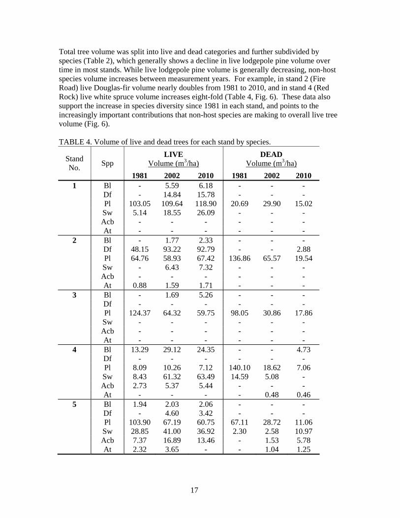
Total tree volume was split into live and dead categories and further subdivided by species (Table 2), which generally shows a decline in live lodgepole pine volume over time in most stands. While live lodgepole pine volume is generally decreasing, non-host species volume increases between measurement years. For example, in stand 2 (Fire Road) live Douglas-fir volume nearly doubles from 1981 to 2010, and in stand 4 (Red Rock) live white spruce volume increases eight-fold (Table 4, Fig. 6). These data also support the increase in species diversity since 1981 in each stand, and points to the increasingly important contributions that non-host species are making to overall live tree volume (Fig. 6). TABLE 4. Volume of live and dead trees for each stand by species.

LIVE Volume (m3/ha)

DEAD Volume (m3/ha) Stand

No. Spp 1981 2002 2010 1981 2002 2010

1 Bl - 5.59 6.18 - - - Df - 14.84 15.78 - - - Pl 103.05 109.64 118.90 20.69 29.90 15.02 Sw 5.14 18.55 26.09 - - - Acb - - - - - - At - - - - - - 2 Bl - 1.77 2.33 - - - Df 48.15 93.22 92.79 - - 2.88 Pl 64.76 58.93 67.42 136.86 65.57 19.54 Sw - 6.43 7.32 - - - Acb - - - - - - At 0.88 1.59 1.71 - - - 3 Bl - 1.69 5.26 - - - Df - - - - - - Pl 124.37 64.32 59.75 98.05 30.86 17.86 Sw - - - - - - Acb - - - - - - At - - - - - - 4 Bl 13.29 29.12 24.35 - - 4.73 Df - - - - - - Pl 8.09 10.26 7.12 140.10 18.62 7.06 Sw 8.43 61.32 63.49 14.59 5.08 - Acb 2.73 5.37 5.44 - - - At - - - - 0.48 0.46 5 Bl 1.94 2.03 2.06 - - - Df - 4.60 3.42 - - - Pl 103.90 67.19 60.75 67.11 28.72 11.06 Sw 28.85 41.00 36.92 2.30 2.58 10.97 Acb 7.37 16.89 13.46 - 1.53 5.78 At 2.32 3.65 - - 1.04 1.25

18

Figure 6. Live volume for each stand by species.

Stand Basal Area Basal area by species illustrates how variable the proportion of live to dead lodgepole pine basal area there is in each stand (Table 5). Stand 4 (Red Rock) has the highest proportion of dead basal area in 1981 (95 percent), followed by stand 5 (U.S. Border) at 78 percent (Table 5). Stand 2 (Fire Road) and stand 3 (Bellevue Look-out) had moderate levels of dead basal area at 66 percent and 43 percent respectively. Stand 1 has the lowest proportion of dead basal area for pine at 16 percent (Table 5). Live basal area for lodgepole pine generally decreased between 1981 and 2010 in most stands (Table 5, Fig. 7). Stand 1 and 4 were exceptions to this, where in stand 1 pine increased slightly, and in

19

stand 4 basal area remained relatively stable (Table 5, Fig. 7). Aside from lodgepole pine, basal area for non-host species generally increased, or stayed the same between 1981 and 2010 (Fig. 7). Depending on the how mixed stands were in terms of composition this resulted in an overall increase in total live basal area (e.g., stand 1) or a decrease (e.g., stand 3) (Fig. 7). These two stands also had the highest and lowest total basal area values in 2010 (Fig. 7). The compensation that non-host species made to overall basal area is quite pronounced in stand 4 which had only 5 m2/ha for live basal area in 1981 but due to substantial increases in subalpine fir and white spruce increased to 14 m2/ha in 2010 (Table 5, Fig. 7). TABLE 5. Basal area of live and dead trees for each stand by species.

LIVE Basal Area (m2/ha)

DEAD Basal Area (m2/ha) Stand

No. Spp. 1981 2002 2010 1981 2002 2010

1 Bl - 1.20 1.20 - - - Df - 2.40 2.40 - - - Pl 19.21 19.21 20.81 3.60 5.60 2.80 Sw 1.20 4.00 5.20 - - - Acb - - - - - - At - - - - - - 2 Bl - 0.40 0.40 - - - Df 6.40 11.20 10.80 - - 0.40 Pl 11.60 10.00 10.80 22.81 11.60 3.20 Sw - 1.20 1.20 - - - Acb - - - - - - At 0.40 0.80 0.80 - - - 3 Bl - 0.40 1.20 - - - Df - - - - - - Pl 21.61 11.60 10.00 16.41 5.60 3.20 Sw - - - - - - Acb - - - - - - At - - - - - - 4 Bl 2.40 4.80 4.00 - - 0.80 Df - - - - - - Pl 1.20 1.60 1.20 22.41 3.20 1.20 Sw 1.20 8.00 8.00 2.40 0.80 - Acb 0.40 0.80 0.80 - - - At - - - 0.40 0.40 5 Bl 0.40 0.40 0.40 - - - Df - 0.40 0.40 - - - Pl 18.01 11.60 10.40 67.11 5.20 2.00 Sw 5.20 6.80 6.00 2.30 0.40 1.60 Acb 1.60 3.60 2.80 - 0.40 1.20 At 0.80 0.80 - - 0.40 0.40

20

Figure 7. Live basal area (m2/ha) for each stand by species.

Changes in Undestorey

Saplings Saplings, or advance regeneration, were defined as trees greater than 1.5 meters in height and less than 7 cm DBH, and were tallied into two size classes: A = 0-3.9 cm DBH and B = 4.0-7.0 cm DBH (Table 6). The density of saplings was highly variable between 2002 and 2010 measurement years, and between stands. For example in stand 5 (U.S. Border) balsam poplar density in size class A went from 40 sph in 2002 to 1220 sph in 2010 (Table 6). In some stands there was an increase in both size classes from 2002 to 2010 (e.g., stand 2), and in others density decreased (e.g., stand 3) (Table 6).

21

TABLE 6. Tree density of live and dead saplings in two size classes (A &B) by species.

LIVE Stems/hectare

DEAD Stems/hectare

2002 2010 2002 2010 Stand No. Spp.

A B A B A B A B 1 Bl - 40 10 - - 80 20 - Df - - - - - - - - Pl 20 - - - 130 110 50 30 Sw 10 10 20 - - 10 - - Acb - - - - - - - - At - - 30 - 10 50 - - 2 Bl - 80 70 30 - 30 - - Df - 90 50 90 10 20 - - Pl 20 20 - - 30 30 - - Sw - - - - 10 - - - Acb - - - - - - - - At 60 200 460 20 40 120 - - 3 Bl 170 100 250 100 10 - 300 - Df 40 20 30 10 - - 30 30 Pl - - - 10 - - - - Sw - - 20 - - - - - Acb - - - - - - - - At - - 40 - - - - - 4 Bl - 130 260 110 - 20 - - Df - - 10 10 - - - - Pl 10 10 10 - 10 110 - - Sw 20 20 50 - - - - - Acb - 70 220 - - - 60 20 At 30 40 150 - - 10 - - 5 Bl 30 20 50 10 40 10 10 - Df - - - - - - - - Pl - - - - 80 - - - Sw - 10 - - - - - - Acb 40 210 1220 - - 20 - - At 60 70 280 - - - - - Wa - 10 - 10 - - - -

A=size class 0-3.9 cm DBH B= size class 4.0-7.0 cm DBH Combining the size classes into a single category reveals that sapling density overall increases from 2002 to 2010 (Fig. 8). For stand 1 (Crandell) it appears as if stand density decreased between measurement years, but this is because there were so many dead

22

saplings (82 percent) recorded in 2002 (Fig. 8). Stands 1 and 5 (U.S. Border) had the lowest sapling density around 110 and 450 live sph respectively. Stands 2, 4 and 5 had the highest density between 700 and 1600 sph in 2010 (Fig. 8). Stand 5 shows the most dramatic increase in live sapling density increasing over 3 times from 2002 at 550 trees/ha to 1560 trees/ha in 2010 (Fig. 8). The species composition of saplings between stands was also highly variable and is noteworthy for the absence of lodgepole pine (Fig. 8). Stand 1 was the only stand that appeared to have a high lodgepole pine component, but 93 percent of these were dead in 2002 and 100 percent were dead in 2010 (Fig. 8). All other stands either had no pine saplings, or a negligible amount. In stand 2 (Fire Road) trembling aspen made up 55 percent of saplings in 2002 and 78 percent in 2010 (Fig. 8); in stand 3 (Bellevue Look-out) subalpine fir accounted for 85 percent and 78 percent of saplings in 2002 and 2010 respectively. Species are more evenly distributed in stand 4 (Red Rock), which was slightly dominated by subalpine fir (31 percent in 2002 and 41 percent in 2010); and stand 5, which was slightly dominated by balsam poplar (30 percent in 2002 and 39 percent in 2010) (Fig. 8).

Regeneration Seedlings were defined as less than or equal to 1.5 meters in height were tallied (live only) by species into four height classes: 0-0.10 m, 0.10-0.50 m, 0.50-1.0 m, 1.0-1.5 m. With the exception of stand 1 (Crandell) regeneration density has increased in all stands between 2002 and 2010. As with the saplings, density of regeneration was extremely variable between stands, size classes and species (Fig. 9). The lowest seedling densities occurred in stand 1 in 2010 (726 sph) and in stand 3 (Bellevue Look-out) in 2002 (269 sph). The highest seedling densities occurred in stand 2 (Fire Road) (7656 sph), and stand 4 (Red Rock) (7524 sph), both in 2010 (Fig. 9). There is no apparent trend between the density of seedlings and size classes, although in each stand one size class tended to dominate (Fig. 9). For example, in stand 2 over 6000 sph occurred in the smallest size class (0-0.10 m) in 2010, of which 83 percent were Douglas-fir. Overall, there was extremely low numbers of the largest seedling class (1.0-1.5 m) (e.g., stands 2, 4 and 5) or it was absent all together (e.g., stands 1 and 3). When this size class was present it accounted for only 1.5 to 3 percent of the total density (Fig. 9 and 10). Lodgepole pine seedlings were only present in stand 2 and stand 3 (66 sph in both stands), accounting for 0.08 and 8 percent, respectively, of the total seedlings density at those sites (Fig. 9). In stand 3 where lodgepole pine seedlings account for 8 percent of the total density they were found growing in extremely open areas where an overstorey canopy was not present (author’s field observations).

23

Figure 8. Live and dead sapling density for each stand (left panel); Live sapling density by species for each stand (right panel). Note: scale of x-axis changes between graphs

24

Figure 9. Live seedling density by height class for each stand (left panel); Live seedling density by species for each stand (right panel).Note: scale of x-axis changes between graphs.

25

Figure 10. Seedling density by height class and species composition. Note: scale of x-axis changes between graphs.

26

Coarse woody debris and fine fuels In 2002, 21 years since MPB mortality, surface fine (< 7.0 cm diameter) woody fuel mass (load) averaged 8.26 tonnes/ha and ranged from 4.94 to 14.2 tonnes/ha (Table 7). Eight years later in 2010, fine woody fuel load averaged 7.34 tonnes/ha and ranged from 6.07 to 11.0 tonnes/ha (Table 7). Stand 2 (Fire Road) had an increase in fine woody fuel load from 2002 to 2010 while stand 4 (Red Rock) remained the same. In the remainder of the stands (1, 3, and 5) fine fuel mass decreased (Table 7). In 2002, coarse woody fuel load (> 7.1 cm diameter) averaged 63.6 tonnes/ha and ranged from 14.3 to 149 tonnes/ha (Table 8). In 2010, coarse woody fuel load averaged 81.9 tonnes/ha and ranged from 29.7 to 172 tonnes/ha (Table 8). All stands had an increase in their coarse woody fuel load from 2002 to 2010, with the highest increase in stand 2 (Fire Road). The overall highest and lowest fuel loads between 2002 and 2010 were in stand 4 (Red Rock) and stand 1 (Crandell), respectively (Fig. 11). In stand 4 the fine fuel load was 5.18 tonnes/ha and the coarse fuel load was 103 tonnes/ha in 2002; in 2010 they were 6.84 tonnes/ha and 137 tonnes/ha, respectively (Fig. 11). In stand 1 the fine fuel load was 8.90 tonnes/ha, and the coarse fuel load was 4.31 tonnes/ha; in 2010 they were 7.12 tonnes/ha and 7.37 tonnes/ha, respectively (Fig. 11). Graphs of average mass and volume of fine and coarse woody fuel load, in 2002 and 2010 can be found in Appendix 2. TABLE 7. Average mass (load) and volume of fine fuels (< 7.0 cm diameter) (all decay classes)

Mass (tonnes/ha) Volume (m3/ha) 2002 2010 2002 2010

Stand Average (std error)

Range Average (std error)



Range

1 8.66 (1.45)

2.98 10.9

6.45 (1.80)

2.48 13.0

20.8 (3.53)

7.03 26.0

15.4 (4.37)

5.86 31.4

2 4.94 (1.09)

1.75 7.52

6.62 (1.22)

3.03 10.3

11.5 (2.55)

4.10 17.6

15.7 (2.94)

7.06 24.6

3 14.2 (1.89)

8.45 18.8

11.0 (2.85)

4.89 21.8

34.2 (4.54)

20.5 45.5

26.4 (6.90)

11.7 52.4

4 6.01 (1.03)

3.86 9.59

6.07 (0.75)

4.40 8.50

14.4 (2.57)

9.18 23.3

14.7 (1.81)

10.7 20.7

5 7.49 (1.88)

4.67 10.1

6.54 (0.88)

4.67 8.81

17.8 (4.57)

11.1 35.4

15.5 (2.10)

11.0 20.7

27

TABLE 8. Average mass (load) and volume of coarse woody debris (> 7.1 cm diameter) (all decay classes)

Mass (tonnes/ha) Volume (m3/ha) 2002 2010 2002 2010

Stand Average (std error) Range Average

(std error) Range Average (std error) Range Average

(std error) Range

1 23.7 (8.52)

4.31 50.3

32.1 (9.54)

7.37 63.8

57.8 (20.8)

10.5 123

79.1 (23.5)

18.1 157

2 14.3 (9.09)

2.47 50.1

29.7 (9.95)

8.59 62.4

34.8 (22.2)

6.02 122

72.5 (24.2)

21.2 152

3 81.1 (7.63)

53.6 94.2

105 (15.6)

65.0 148

198 (18.6)

131 230

258 (38.4)

160 364

4 149 (63.7)

66.0 401

172 (65.1)

83.7 430

365 (155)

161 979

429 (161)

211 1069

5 49.4 (10.5)

13.8 69.4

70.7 (15.9)

15.6 114

120 (25.7)

33.6 169

174 (38.8)

39.4 281

Figure 11. Top panel: Stand 4 (Red Rock) plot 5 fuel transect; photograph on the left is 2002 and on right is 2010. Bottom panel: Stand 1 (Crandell) plot 1 fuel transect; photograph on the left is 2002 and on the right is 2010. In 2002 photographs were taken after light snow and vegetation curing in late October, and in 2010 were taken at full green-up in early September.

28

Dendroecology

Cross-Dated Series Lodgepole pine tree-ring chronologies were developed for each stand. If dominant or co-dominant non-host species (e.g., Douglas-fir, white spruce) were present chronologies were also developed for those species, though much fewer samples were collected. Cross-dating statistics were computed for each tree-ring series including: series range, number of cores collected, inter-series correlation, and mean sensitivity (Table 9). The inter-series correlation measures the degree of agreement between a series and the master chronology, and represents how much common stand-level signal is recorded (Grissino-Mayer 2001). The level of correlation among correctly cross-dated tree-ring series may differ with tree species, geographic area, site homogeneity, amount of stand competition, and degree of disturbance (Grissino-Mayer 2001). The average inter-series correlation for lodgepole pine was 0.54, which is typical of the species, and is well above the minimum values of 0.33 (p<0.001), indicating that lodgepole pine trees within stands shared a common growth signal (Table 9). The lowest correlation was for white spruce in stand 5 (r = 0.47), which is likely a result of the low number of cores sampled in this stand (Table 9). Mean sensitivity, a statistic measuring the mean relative change between the adjacent ring widths (Fritts 1976), is a metric of how complacent or sensitive a tree-ring series is, which is largely determined by how much tree growth is limited by environmental factors. In general, the mean sensitivity of the tree-ring series is moderate (0.21 to 0.29) indicating that yearly tree-ring variability is reasonably responsive to environmental factors at the selected locations. Standardized tree-ring chronologies were developed for each measurement series in each stand (Appendix 3). TABLE 9. Cross-dating statistics for host and non-host tree-rings series

Stand No.

Stand Name Spp.

No. of dated series

Master Series

Series inter-correlation

Mean Sensitivity

1 Crandell Pl 31 1864 - 2010 0.52 0.25 Fire Road Pl 26 1897 - 2010 0.60 0.23 2 Fire Road Df 7 1903 - 2010 0.48 0.23

3 Bellevue- Lookout Pl 27 1878 - 2010 0.55 0.22

Red Rock Pl 29 1866 - 2010 0.50 0.24 4

Red Rock Sw 6 1881 - 2010 0.52 0.29 U.S. Border Pl 27 1880 - 2010 0.53 0.23

5 U.S. Border Sw 5 1898 - 2010 0.47 0.21

Cohort Ages Average tree ages are complied for lodgepole pine and non-host species from all the samples collected (i.e., increment cores, CWD discs, and sapling cookies) (Table 10). All

29

non-host ages were averaged across species. Increment cores were collected at breast height and average ages were not corrected. CWD, which was only collected for lodgepole pine, was collected from tree base and is a good representation of total tree age, and thus establishment (Table 10). Lodgepole pine ages based on increment cores vary from 94 years old (stand 2) to 125 years old (stand 4); for non-host species range from 51 years old (stand 3) to 104 years old (stand 5) (Table 10). The average ages of lodgepole pine based on CWD samples are less variable than ages based on increment cores, with the exception of stand 1 which has a standard error of 9.0, and ranges from 83 to 119 years old (Table 10). Lodgepole pine saplings were very difficult to obtain in each stand, which is why in stand 4 no standard error or range statistics could be calculated. Pine saplings tended to only grow in large gaps or on the edge of old roads; their ages are extremely variable, ranging from 16 years old (stand 3) to 78 years old (stand 2) (Table 10). Non-host species, the most abundant of which were subalpine fir and white spruce, almost all had average ages between 20 to 29 years old, with the exception of stand 5 which had an average ages of 41 years old (Table 10). TABLE 10. Age data for overstorey based on increment cores and CWD discs; and for understorey based on sapling cookies.

Stand No. Lodgepole pine age (years) Non-host age* (years)

Increment cores+

Average (std error) Range Average

(std error) Range

1 112 (5.0) 53 - 140 61 (5.8) 41 - 88 2 94 (3.5) 71 - 117 90 (4.7) 66 - 111 3 114 (2.6) 92 - 134 51 (8.0) 43 - 59 4 125 (3.3) 80 - 144 91 (8.4) 17 - 132 5 107 (3.2) 82 - 126 104 (3.6) 90 -112

CWD


(std error) Range

1 119 (9.0) 83 - 119 - - 2 124 (1.3) 118 - 131 - - 3 120 (1.7) 107 - 126 - - 4 136 (3.2) 108 - 143 - - 5 125 (1.2) 116 - 130 - -

Saplings


(std error) Range

1 62 (2.5) 59 - 64 29 (1.7) 18 - 49 2 78 (1.0) 77 - 78 23 (1.4) 12 - 40 3 16 (1.8) 11 - 20 21 (1.6) 10 - 44 4 20 (-) - 25 (1.0) 16 - 35 5 72 (2.5) 69 - 74 41 (3.0) 19 - 65

* Non-host species include: subalpine fir, Douglas-fir, and white spruce + Age at breast height

30

Disturbance History To unravel the stand dynamics of each stand we present all of the tree-ring data in an integrated graphical form: timing of canopy establishment, growth releases, CWD death date, and establishment dates of advance regeneration (Fig. 12 through 16). Pith dates of CWD collected from the tree base provides the best estimation of lodgepole pine establishment. Stands 1 (Crandell) and 4 (Red Rock), which are geographically closest to one another (see Fig. 1) were the most variable in the timing of overstorey establishment. In stand 1 there was a small pulse establishment in 1860-1870, but establishment continued sporadically until the 1940s for pine and the 1970s for subalpine fir, Douglas-fir and spruce (Fig. 12a). Stand 4 had a fairly large pulse of establishment in 1860-1870, followed by low levels of continuous establishment until 1920; thereafter subalpine fir established sporadically until around 1980 (Fig. 15a). Stands 2 (Fire Road), 3 (Bellevue Look-out) and 5 (U.S. Border) had a more discrete pulse of establishment for lodgepole pine (based on CWD), which mainly occurred between 1880 and 1890 (Fig. 13a, 14a, 16a). Stands 3 and 5 had the most classically “even-aged” overstorey distributions; large pulses of establishment of pine occurred in 1890 in stand 3 (Fig. 14a) and in 1880 in stand 5 (Fig. 16a). Similar to stands 1 and 4, establishment of non-host species in these stands occurred in a sporadic way from the late-1800s to the mid-1900s. While most stands had a number of non-host species establishing at the same time as pine, stand 3 is noteworthy for being nearly pure lodgepole pine until the 1950s, when some subalpine fir started to establish (Fig. 14a). When non-host species were present they were commonly subalpine fir, Douglas-fir and white spruce (see results above), but in stand 2 there was also a minor co-dominant to intermediate cohort of whitebark pine (Pinus albicaulis), which established in two phases in 1910 and 1940 (Fig. 13a). Significant growth releases (>20 percent of trees recording a 25 percent increase in radial growth) were recorded in the lodgepole pine and non-host species (if present) in all stands (Fig. 12b to 16b). The earliest growth release detected started in the 1890s in stand 1 (Fig. 12b) and stand 4 (Fig. 15b). It is interesting to note that these releases occurred in stands with the most sporadic establishment history (see above). The next significant growth release occurred in the 1940s in all stands, with the exception of stand 2 (fewer than 20 percent of trees recorded release) (Fig. 13b). The 1940s release was most pronounced in stand 4 where over 60 percent of the pine and over 40 percent of the spruce recorded the release for at least 10 years (Fig. 15b). In stand 1 around 40 percent of the pine underwent a release (Fig. 12b), and in the other stands between 20 and 30 percent of trees recorded a growth release during this period. The final significant growth release, and the strongest, occurred in the late 1980s and 1990s in all stands (Fig. 12b to 16b). This growth release occurred after documented outbreaks of MPB in the park, and between 30 to 90 percent of pine and non-host species recorded sustained releases. In stand 3, the purest pine stand in the group, around 50 percent of trees recorded a growth release until 1994 (Fig. 14b). In stands 2 and 4 between 60 to 90 percent of Douglas-fir and white spruce recorded sustained releases well into the 1990s as well (Fig. 13b2 and Fig.15b2).

31

Mortality of the coarse woody debris was strongly centered around 1980 and 1990 for all stands, with the exception of stand 1. The major pulse of CWD mortality in stands 2 through 5 (Fig. 13c through 16c) proceeded or was coincident with major canopy releases during the 1980s and 1990s. In stand 1, CWD mortality occurred on a fairly continuous basis (Fig. 12c). This is likely because it was very difficult to obtain large pieces of CWD in this stand, resulting in the collection of smaller diameter samples, which probably died as a result of stand thinning. The understorey was comprised almost solely of shade tolerant species such as subalpine fir and white spruce (Fig. 12d through 16d) that established in a pulse that peaked in the 1980s or the 1990s. These establishment pulses were slightly lagged behind canopy releases and CWD mortality dates. In stands where pine was present it generally established outside of the dominant regeneration pulse. For example, in stand 1 pine established in the 1940s (Fig. 12d), and in stand 2 in the1930s and 1940s (Fig. 13d). Stand 5 is the one stand where advance regeneration did not appear to establish as a pulse within a few decades, but instead established beginning in the 1930s and continued fairly uniformly until 1990 (Fig 16d).

Figure 12. Reconstruction for stand 1 (Crandell): (a) Date of establishment of the overstorey; (b) Percent of lodgepole pine showing growth releases in a given year (left-axis), and sample depth (right-axis); (c) death dates of coarse woody debris; (d) Date of establishment of advance regeneration in the understorey. *Increment cores collected at breast height.

32

Figure 13. Reconstruction for stand 2 (Fire Road): (a) Date of establishment of the overstorey; (b) Percent of lodgepole pine (b1) and Douglas-fir (b2) showing growth releases in a given year (left-axis), and sample depth (right-axis); (c) death dates of coarse woody debris; (d) Date of establishment of advance regeneration in the understorey. *Increment cores collected at breast height.

33

Figure 14. Reconstruction for stand 3 (Bellevue Look-out): (a) Date of establishment of the overstorey; (b) Percent of lodgepole pine showing growth releases in a given year (left-axis), and sample depth (right-axis); (c) death dates of coarse woody debris; (d) Date of establishment of advance regeneration in the understorey. *Increment cores collected at breast height.

34

Figure 15. Reconstruction for stand 4 (Red Rock): (a) Date of establishment of the overstorey; (b) Percent of lodgepole pine (b1) and white spruce (b2) showing growth releases in a given year (left-axis), and sample depth (right-axis); (c) death dates of coarse woody debris; (d) Date of establishment of advance regeneration in the understorey. *Increment cores collected at breast height.

35

Figure 16. Reconstruction for stand 5 (U.S. Border): (a) Date of establishment of the overstorey; (b) Percent of lodgepole pine (b1) and white spruce (b2) showing growth releases in a given year (left-axis), and sample depth (right-axis); (c) death dates of coarse woody debris; (d) Date of establishment of advance regeneration in the understorey. *Increment cores collected at breast height. Integration of Tree-ring Chronologies Standardized tree-ring chronologies collected in this study were integrated with those collected in the 2008-09 in the northern Foothills (Nordegg to Grande Prairie) (Alfaro et al. 2009), and those collected around Banff and Jasper in previous studies (Alfaro et al. 2006), resulting in a total of 28 lodgepole pine chronologies spanning over 5 degrees of latitude (see Fig. 1). Factor Analysis was performed on the common period: 1908-2003

36

and resulted in six components with an eigenvalue greater than or equal to 1.0, cumulatively explaining 76 percent of the total variability of the dataset (Table 11). TABLE 11. Results of Factor Analysis of 28 lodgepole pine chronologies.

Component Eigenvalue % Total variance Cumulative % 1 7.535635 26.91298 26.9130 2 4.556212 16.27219 43.1852 3 3.922984 14.01066 57.1958 4 2.230253 7.96519 65.1610 5 1.905890 6.80675 71.9678 6 1.166434 4.16584 76.1336

The following chronologies had a coefficient of variation of >0.70, an indication of how strongly the chronology loaded onto each factor:

• Factor chronology 1 (FC 1): SRD 55, 56, 60, 61, 63, 65 (Lower Foothills PSPs) • Factor chronology 2 (FC 2): CR, FR, BV, RR, USB (Waterton PSPs) • Factor chronology 3 (FC 3): B2, BL3 (Banff-Blairmore) • Factor chronology 4 (FC 4): J1, J2 (Jasper) • Factor chronology 5 (FC 5): H2 (Upper Foothills PSP) • Factor chronology 6 (FC 6): S105, S111, J3 (Subalpine PSPs)

The factor loadings suggest that conditions controlling radial growth are strongly related to geographic and sub-regional conditions within the study area. FC 1 explained 27 percent of the total variance (Table 11), and was loaded by the most northern chronologies (see Fig. 1) in the Lower Foothills natural sub-region (S55 to S65) (Fig.17). The annual growth pattern for FC1 has below average growth until around 1930 when there is an abrupt shift to above average growth, which peaks around 1935. Growth remains above average until the early 1980s when there is a switch to below average growth until the mid-1990s (Fig. 17). FC 2 explained 16.3 percent of the total variance (Table 11) and was loaded by all of the WLNP stands (1 through 5) in the Montane natural sub-region (Fig. 17). This factor chronology is dominated by a decadal signal of high amplitude variance around the mean. Two peaks dominate the time series, one in the 1920-30s and the other in the 1980s-90s (Fig. 17). FC 3 explained 14 percent of the total variance (Table 11) and is loaded by a southern Banff chronology and a chronology from the Blairmore area (see Fig. 1). These chronologies are also located in the Montane natural sub-region but are at a higher elevation than the Waterton Lakes chronologies (results not shown). This factor chronology has a curious growth pattern of above average growth from 1908 to 1930, where after growth plummets to a low in 1940, followed by a gradual recovery (Fig. 17). FC 4 explained 8 percent of the total variance (Table 11) and was loaded by chronologies in the Jasper area (see Fig. 1). Annual growth in FC 4 is dominated by a gradual decrease in growth over time, appearing to be senesce signal, but with two periods of growth recovery in the 1980s and 1990s (Fig. 17). FC 5 explained 6.8 percent of the total variance (Table 11) and was loaded by a single chronology, H2 (see Fig. 1), in the Upper Foothills natural sub-region. This factor is characterized by average

37

growth until the 1960s when a sustained period of above average growth occurs, ending abruptly around 1990 when growth declines below the average (Fig. 17). Finally, FC 6 explained 4.2 percent of the total variance (Table 11) and was loaded by chronologies in the Nordegg and Jasper region in the Subalpine natural sub-region (see Fig. 1). This factor chronology appears to have a multi-decadal signal that is characterized by a large growth pulse centered on the 1940s and sustained above average growth from the 1980s until the end of the series (Fig. 17).

Figure 17. Factor chronologies from twenty-eight lodgepole pine chronologies collected in the Alberta Foothills; percent variance explained by each factor in brackets. Black line is tree-ring index and red line is a 15-yr spline.

38

Discussion

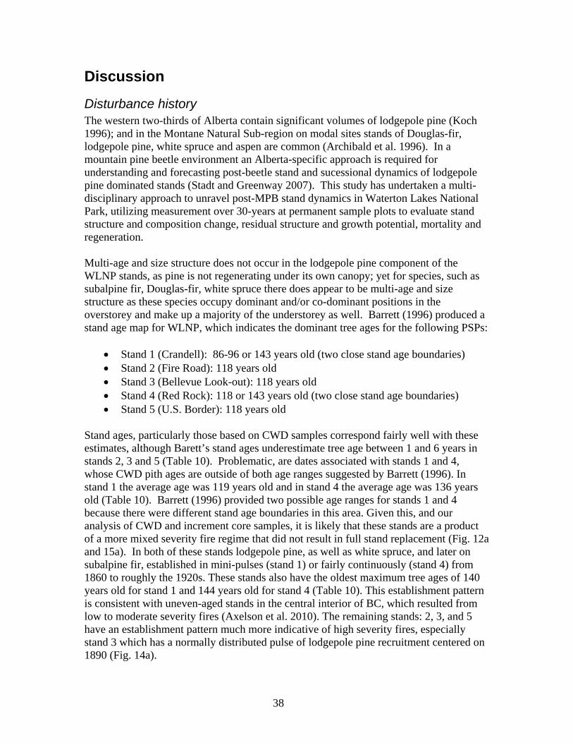
Disturbance history The western two-thirds of Alberta contain significant volumes of lodgepole pine (Koch 1996); and in the Montane Natural Sub-region on modal sites stands of Douglas-fir, lodgepole pine, white spruce and aspen are common (Archibald et al. 1996). In a mountain pine beetle environment an Alberta-specific approach is required for understanding and forecasting post-beetle stand and sucessional dynamics of lodgepole pine dominated stands (Stadt and Greenway 2007). This study has undertaken a multi-disciplinary approach to unravel post-MPB stand dynamics in Waterton Lakes National Park, utilizing measurement over 30-years at permanent sample plots to evaluate stand structure and composition change, residual structure and growth potential, mortality and regeneration. Multi-age and size structure does not occur in the lodgepole pine component of the WLNP stands, as pine is not regenerating under its own canopy; yet for species, such as subalpine fir, Douglas-fir, white spruce there does appear to be multi-age and size structure as these species occupy dominant and/or co-dominant positions in the overstorey and make up a majority of the understorey as well. Barrett (1996) produced a stand age map for WLNP, which indicates the dominant tree ages for the following PSPs:

• Stand 1 (Crandell): 86-96 or 143 years old (two close stand age boundaries) • Stand 2 (Fire Road): 118 years old • Stand 3 (Bellevue Look-out): 118 years old • Stand 4 (Red Rock): 118 or 143 years old (two close stand age boundaries) • Stand 5 (U.S. Border): 118 years old

Stand ages, particularly those based on CWD samples correspond fairly well with these estimates, although Barett’s stand ages underestimate tree age between 1 and 6 years in stands 2, 3 and 5 (Table 10). Problematic, are dates associated with stands 1 and 4, whose CWD pith ages are outside of both age ranges suggested by Barrett (1996). In stand 1 the average age was 119 years old and in stand 4 the average age was 136 years old (Table 10). Barrett (1996) provided two possible age ranges for stands 1 and 4 because there were different stand age boundaries in this area. Given this, and our analysis of CWD and increment core samples, it is likely that these stands are a product of a more mixed severity fire regime that did not result in full stand replacement (Fig. 12a and 15a). In both of these stands lodgepole pine, as well as white spruce, and later on subalpine fir, established in mini-pulses (stand 1) or fairly continuously (stand 4) from 1860 to roughly the 1920s. These stands also have the oldest maximum tree ages of 140 years old for stand 1 and 144 years old for stand 4 (Table 10). This establishment pattern is consistent with uneven-aged stands in the central interior of BC, which resulted from low to moderate severity fires (Axelson et al. 2010). The remaining stands: 2, 3, and 5 have an establishment pattern much more indicative of high severity fires, especially stand 3 which has a normally distributed pulse of lodgepole pine recruitment centered on 1890 (Fig. 14a).

39

Overstorey mortality and stocking The mountain pine beetle, which was first detected in the park in 1977 cumulatively resulted in over 1 million m3 of lodgepole pine mortality from 1977 to 1987 (Brandt and Amirault 1994) in southwestern Alberta. Based on average tree ages this made the dominant lodgepole pine cohort between 80 to 100 years old at the time of the outbreak, making them highly susceptible to successful MPB attack (Safranyik and Carroll 2006). Before the outbreak, lodgepole pine was the dominate species in all of the stands, making up 89 percent of the canopy in the early 1980s (Hawkes et al. 2004b). After the outbreak, the average proportion of lodgepole pine dropped to 59 percent in 2002 and to 54 percent in 2010. With a nearly 40 percent reduction in the pine cohort the proportion of non-host trees: white spruce, subalpine fir, and Douglas-fir was 16, 15 and 7 percent, respectively, of the total species composition in 2010 (Table 1, Fig. 4). Over the course of the MPB outbreak total live tree density declined over the period 1981 to 2002, falling from 859 sph to 681 sph, and to 608 sph in 2010 (Table 2; Fig. 4). In 1981, lodgepole pine mortality averaged across stands was 44 percent, but ranged between 93 percent (stand 4) to 10 percent (stand 1). In stands 2 through 5 lodgepole pine volume dramatically decreased, and volumes of dead pine ranged between 67 to 120 m3/ha was dead (Table 4). In terms of basal area, this represents between 43 to 95 percent that was dead (Table 5). The exception to this was in stand 1, where lodgepole pine volume increased slightly (Fig. 5), and only 15 percent of total basal area was dead (Table 5), corresponding to very low overall mortality in this stand across measurement years.

Canopy response When canopy dominants die as a result of successful MPB attack, younger trees, both surviving lodgepole pine and non-host species, may respond to the increase in resources available for growth with a period of accelerated growth. Growth releases were recorded in the tree-ring record during the 1970s outbreak in each stand. Although it would seem that a direct link should exist between the amount of mortality or the percentage of dead basal area and the proportion of trees undergoing a release there generally is not a clear relationship. For example, in stand 1, which had very low mortality in 1981 and low levels of basal area loss (15 percent) up to 60 percent of the stand recorded a sustained growth release in the 1980s (Fig. 12b). Conversely, in stand 4, which had up to 93 percent mortality, fewer trees (~ 40 percent) recorded a growth release during the 1980s, although nearly 100 percent of the non-host spruce underwent a sustained growth release (Fig. 15b). This highlights how stand conditions, such as canopy closure and/or tree vigour may influence the ability of residual trees to take advantage of increased resources in response to a canopy disturbance. Given that these factors are likely to impact growth releases it must be stressed that stands 1 and 4 are somewhat anomalous in that they represented uneven-aged and mixed species stands before the MPB outbreaks. For stand 2, 3 and 5, which were more even-aged and dominated by lodgepole pine there is a clearer relationship between canopy mortality, loss of basal area and proportion of trees releasing. For example, in stand 5 where 78 percent of the basal area was dead in 1981 between 60 and 80 percent of the residual lodgepole pine experienced a sustained growth release (Fig. 16b). Unlike stand 4, the white spruce component of this stand only

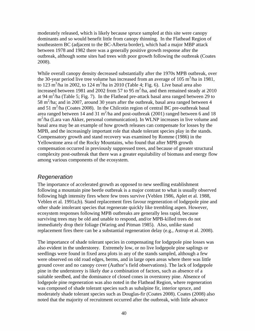
40

moderately released, which is likely because spruce sampled at this site were canopy dominants and so would benefit little from canopy thinning. In the Flathead Region of southeastern BC (adjacent to the BC-Alberta border), which had a major MBP attack between 1978 and 1982 there was a generally positive growth response after the outbreak, although some sites had trees with poor growth following the outbreak (Coates 2008). While overall canopy density decreased substantially after the 1970s MPB outbreak, over the 30-year period live tree volume has increased from an average of 105 m3/ha in 1981, to 123 m3/ha in 2002, to 124 m3/ha in 2010 (Table 4; Fig. 6). Live basal area also increased between 1981 and 2002 from 57 to 95 m2/ha, and then remained steady at 2010 at 94 m2/ha (Table 5; Fig. 7). In the Flathead pre-attack basal area ranged between 29 to 58 m2/ha; and in 2007, around 30 years after the outbreak, basal area ranged between 4 and 51 m2/ha (Coates 2008). In the Chilcotin region of central BC pre-outbreak basal area ranged between 14 and 31 m2/ha and post-outbreak (2001) ranged between 6 and 18 m2/ha (Lara van Akker, personal communication). In WLNP increases in live volume and basal area may be an example of how growth releases can compensate for losses by the MPB, and the increasingly important role that shade tolerant species play in the stands. Compensatory growth and stand recovery was examined by Romme (1986) in the Yellowstone area of the Rocky Mountains, who found that after MPB growth compensation occurred in previously suppressed trees, and because of greater structural complexity post-outbreak that there was a greater equitability of biomass and energy flow among various components of the ecosystem.

Regeneration The importance of accelerated growth as opposed to new seedling establishment following a mountain pine beetle outbreak is a major contrast to what is usually observed following high intensity fires where few trees survive (Veblen 1986, Aplet et al. 1988, Veblen et al. 1991a;b). Stand replacement fires favour regeneration of lodgepole pine and other shade intolerant species that regenerate quickly like trembling aspen. However, ecosystem responses following MPB outbreaks are generally less rapid, because surviving trees may be old and unable to respond, and/or MPB-killed trees do not immediately drop their foliage (Waring and Pitman 1985). Also, unlike stand replacement fires there can be a substantial regeneration delay (e.g., Astrup et al. 2008). The importance of shade tolerant species in compensating for lodgepole pine losses was also evident in the understorey. Extremely low, or no live lodgepole pine saplings or seedlings were found in fixed area plots in any of the stands sampled, although a few were observed on old road edges, berms, and in large open areas where there was little ground cover and no canopy cover (Author’s field observations). The lack of lodgepole pine in the understorey is likely due a combination of factors, such as absence of a suitable seedbed, and the dominance of closed cones in overstorey pine. Absence of lodgepole pine regeneration was also noted in the Flathead Region, where regeneration was composed of shade tolerant species such as subalpine fir, interior spruce, and moderately shade tolerant species such as Douglas-fir (Coates 2008). Coates (2008) also noted that the majority of recruitment occurred after the outbreak, with little advance

41

regeneration present in the stands before the outbreak occurred. In WLNP we unfortunately do no have density data for regeneration in the 1980s, although establishment data based on understorey dating generally supports this as most stands experienced a recruitment pulse after the MPB outbreak (Fig. 12d through 16d). Regeneration densities were highly variable between measurement years (2002 and 2010) and between stands: advance regeneration densities ranged from 350 to 800 sph in 2002; and 450 to 1600 sph in 2010 (Fig. 8). Seedling densities ranged from 250 to 4000 sph in 2002; and around 750 to 7800 sph in 2010 (Fig. 9). In the Flathead, total recruitment was also highly variable ranging between 500 sph to 12,000 sph (Coates 2008), and in the southern interior of BC sapling and seedling densities ranged between < 500 sph to over 20,000 sph (Vyse et al. 2009). Vyse et al. (2009) note that the highest densities of advance regeneration were found in the wetter biogeoclimatic zones at high elevation, and almost all regeneration was subalpine fir.

Fuels Fine fuels changed very little between 2002 and 2010 measurement years. Stand 2 (Fire Road) was the only stand that had an increase in fine woody fuel load (Table 7, Appendix 2); this stand had the highest reduction in standing dead pine from 2002 to 2010 (50 percent to 22 percent), and the additional branchwood, now on the ground, probably contributed to this increase in fine woody fuel load (Table 3). Page and Jenkins (2007) reported fine woody fuel load (< 7.6cm) of 14.4 tonnes/ha in a Utah lodgepole pine stand with 71 to 89 percent mortality 20 years after a mountain pine beetle outbreak. Fine fuel load in this study measured in 2002 (21 years after the MPB outbreak) averaged 12.1 tonnes/ha and ranged from 5.88 to 16.7 tonnes/ha (Table 7). In the WLNP stands mortality in lodgepole pine ranged from 10 to 93 percent, averaging 44 percent less than reported in Page and Jenkins (2007). Simard et al. (2011) measured fine and coarse woody loads in lodgepole pine stands in Yellowstone National Park 29 to 36 years after a MPB outbreak, with an average mortality of 62 percent and mortality levels ranging from 50 to 82 percent. In Yellowstone, fine woody fuel load was estimated at 12.5 tonnes/ha. In this study, 30 years after beetle outbreak (2010 measurement), fine woody fuel load averaged 7.34 tonnes/ha and ranged from 6.07 to 11.0 tonnes/ha (Table 7). The difference in fine fuels load is likely due to the fact that average mortality in Yellowstone was 62 percent (Simard et al. 2011) as compared to average morality of 44 percent in WLNP. All of the stands had an increase in coarse woody fuel load from 2002 to 2010, with the highest increase in stand 2 (Fire Road), which coincides with large reductions in standing dead pine from 2002 to 2010. Stand 2 had the greatest change in standing dead lodgepole pine, going from 50 percent in 2002 to 22 percent in 2010 (Table 3). This change in structure from standing to down has contributed to the increase coarse woody fuel loads. Page and Jenkins (2007) reported coarse woody fuel load (> 7.6cm) of 101 tonnes/ha in post-beetle stand in Utah. In this study, coarse woody fuel load averaged 63.6 tonnes/ha and ranged up to 149 tonnes/ha in 2002 (Table 8). A likely difference in average coarse fuel loads is due to overall lower beetle caused mortality in the WLNP stands as compared to those in Utah (Page and Jenkins 2007). In their study, Simard et al. (2011) estimated coarse woody fuel load in the 35 years since beetle outbreak at 50.7 tonnes/ha with a range of 9.27 to 88.0 tonnes/ha. Their study stands had an average of 62 percent

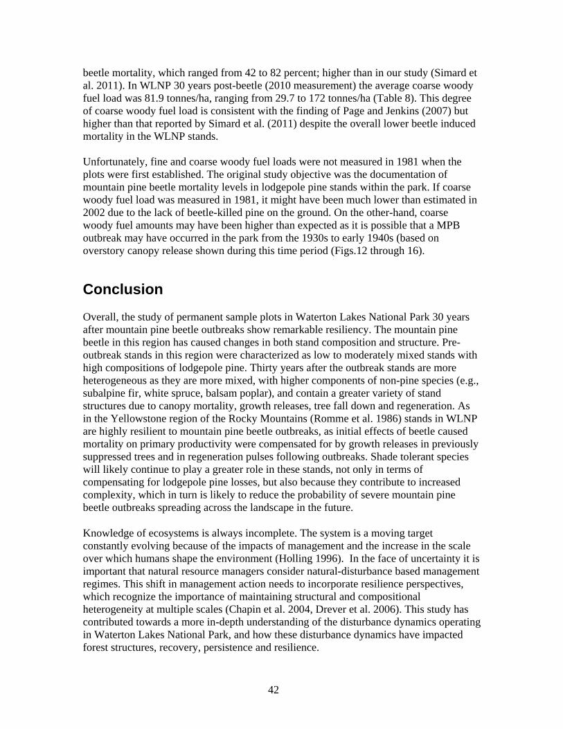
42

beetle mortality, which ranged from 42 to 82 percent; higher than in our study (Simard et al. 2011). In WLNP 30 years post-beetle (2010 measurement) the average coarse woody fuel load was 81.9 tonnes/ha, ranging from 29.7 to 172 tonnes/ha (Table 8). This degree of coarse woody fuel load is consistent with the finding of Page and Jenkins (2007) but higher than that reported by Simard et al. (2011) despite the overall lower beetle induced mortality in the WLNP stands. Unfortunately, fine and coarse woody fuel loads were not measured in 1981 when the plots were first established. The original study objective was the documentation of mountain pine beetle mortality levels in lodgepole pine stands within the park. If coarse woody fuel load was measured in 1981, it might have been much lower than estimated in 2002 due to the lack of beetle-killed pine on the ground. On the other-hand, coarse woody fuel amounts may have been higher than expected as it is possible that a MPB outbreak may have occurred in the park from the 1930s to early 1940s (based on overstory canopy release shown during this time period (Figs.12 through 16).

Conclusion

Overall, the study of permanent sample plots in Waterton Lakes National Park 30 years after mountain pine beetle outbreaks show remarkable resiliency. The mountain pine beetle in this region has caused changes in both stand composition and structure. Pre-outbreak stands in this region were characterized as low to moderately mixed stands with high compositions of lodgepole pine. Thirty years after the outbreak stands are more heterogeneous as they are more mixed, with higher components of non-pine species (e.g., subalpine fir, white spruce, balsam poplar), and contain a greater variety of stand structures due to canopy mortality, growth releases, tree fall down and regeneration. As in the Yellowstone region of the Rocky Mountains (Romme et al. 1986) stands in WLNP are highly resilient to mountain pine beetle outbreaks, as initial effects of beetle caused mortality on primary productivity were compensated for by growth releases in previously suppressed trees and in regeneration pulses following outbreaks. Shade tolerant species will likely continue to play a greater role in these stands, not only in terms of compensating for lodgepole pine losses, but also because they contribute to increased complexity, which in turn is likely to reduce the probability of severe mountain pine beetle outbreaks spreading across the landscape in the future.

Knowledge of ecosystems is always incomplete. The system is a moving target constantly evolving because of the impacts of management and the increase in the scale over which humans shape the environment (Holling 1996). In the face of uncertainty it is important that natural resource managers consider natural-disturbance based management regimes. This shift in management action needs to incorporate resilience perspectives, which recognize the importance of maintaining structural and compositional heterogeneity at multiple scales (Chapin et al. 2004, Drever et al. 2006). This study has contributed towards a more in-depth understanding of the disturbance dynamics operating in Waterton Lakes National Park, and how these disturbance dynamics have impacted forest structures, recovery, persistence and resilience.

43

Acknowledgements We would like to acknowledge the Foothills Research Institute Mountain Pine Beetle Ecology Program and the Canadian Forest Service Mountain Pine Beetle Initiative Fund for jointly funding this project. Field assistance was provided by George Dalrymple and Vince Waring. Analytical support was provided by Lara van Akker and Chris Stockdale, who originally wrote the SAS scripts used in this study. Thanks go to a number of folks at Waterton Lakes National Park. Rob Watt assisted Dr. Moody in plot establishment in 1981 and had the foresight to create copies of all original field forms that were used to re-locate the plots in 2002. Cyndi Smith and Barb Johnston assisted with park research permits and field logistics. Thanks to Waterton Lake National Park for providing accommodation in their research house during fieldwork.

References Agee, J.K. 1993. Fire ecology of Pacific Northwest forests. Island Press, Washington,

D.C. Alberta Environmental Protection. 1994. Natural regions and sub-regions of Alberta.

Alberta Environment, Edmonton, Alberta. Pub. No. 1/531. Alberta Sustainable Resource Development. 2005. Edmonton, Alberta.

http://www.gov.ab.ca/acn/200503/17742C557B758-7B63-4923-89CB67EF2EE5D1EB.html

Alberta Sustainable Resource Development. 2007. Mountain Pine Beetle Management Strategy. Pub No. T/154. Alberta Sustainable Resources Development, Edmonton, Alberta, Canada, 20p.

Alfaro, R., Campbell, R., Vera, P., Hawkes, B., Shore, T. 2004. Dendroecological reconstruction of mountain pine beetle outbreaks in the Chilcotin Plateau of British Columbia. In: Mountain Pine Beetle Symposium: Challenges and solutions (Eds. T.L. Shore, J.E. Brooks and J.E. Stone), pp. 245-256, Natural Resources Canada, Canadian Forest Service, Pac. For. Centre, Victoria, B.C., Canada. Inf. Rep. B.C.-X-399, 287 p.

Alfaro, R. Campbell, E., and Hawkes, B. 2006. Historical Frequency, Intensity and Extent of Mountain Pine Beetle Disturbance in Landscapes of British Columbia. Canadian Forest Service, Pacific Forestry Centre, Victoria, BC, MPBI Project # 2.05, 139 p.

Alfaro, R., Axelson, J., and Hawkes, B. 2009. Decision Support for Forest Management in a Mountain Pine Beetle Environment: The dendroecology and stand dynamics of a selection of Permanent Sample Plots, Alberta, Canada. Final Report to Mountain Pine Beetle Ecology Program, Foothills Research Institute. 52pp.

Alfaro, R., Axelson, J., Hawkes, B. 2009. Decision Support for Forest Management in a Mountain Pine Beetle Environment: The dendroecology and stand dynamics of a selection of Permanent Sample Plots, Alberta, Canada. Final Report to Mountain Pine Beetle Ecology Program, Foothills Research Institute. 52pp.

44

Aplet, G.H.; Laven, R.D.; Smith, F.W. 1988. Patterns of community dynamics in Colorado, USA Engelmann spruce-subalpine for forests. Ecology 69 (2):312-319.

Archibald, J.H., Klappstein, G.D., Corns, I.G. 1996. Field guide to ecosites of southwestern Alberta. Canadian Forest Service, Northern Forestry Centre, Edmonton Alberta.

Astrup, R., Coates, D.K., Hall, E. 2008. Recruitment limitation in forests: Lessons from an unprecedented mountain pine beetle epidemic. Forest Ecology and Management, 256(10): 1743-1750.

Axelson J., Alfaro, R., Hawkes, B. 2009. Influence of fire and mountain pine beetle on the dynamics of lodgepole pine stands in British Columbia, Canada, Forest Ecology and Management, Vol.257, Issue 9: 1874-1882. doi: 10.1016/j.foreco.2009.01.047.

Axelson J., Alfaro, R., Hawkes, B. 2010. Changes in stand structure in uneven-aged lodgepole pine stands impacted by mountain pine beetle epidemics and fires in central British Columbia. The Forestry Chronicle, 86(1): 87-99.

BC Ministry of Forests and Range. 2010. Field manual for describing terrestrial ecosystems, 2nd ed. Land management handbook, 0229-1622;25. ISBN 978-0-7726-6357-3 (PDF).

Barrett, S.W. 1996. The historic role of fire in Waterton Lakes National Park, Alberta. Contract report, Parks Canada Contract No. KWL 30004, April 1996 26 pages plus appendices.

Berg, E., Henry, D., Fastie, C., De Volder, A., Matsuoka, S. 2006. Spruce beetle outbreaks on the Kenai Peninsula, Alaska, and Kluane National Park and Reserve, Yukon Territory: Relationship to summer temperatures and regional differences in disturbance regimes. Forest Ecology Management, 227: 219-232.

Brandt, J.P., Amirault, P. 1994. Forest insect- and disease-caused depletions to forests of west-central Canada: 1982-87. Natural Resources Canada, Canadian Forest Service, Northern Forest Centre, Edmonton, Alberta. Inf. Rep. NOR-X-333.

Campbell, E., Alfaro, R., Hawkes, B. 2007. Spatial distribution of mountain pine beetle outbreaks in relation to climate and stand characteristics: A dendroecological analysis. Journal of Integrated Plant Biology, 49(2): 168-178.

Chapin III, S.F., Callaghan, T.V., Bergeron, Y., Fukuda, M., Johnstone, J.F., Juday, G., Zimov, S.A. 2004. Global change and the boreal forest: thresholds, shifting states or gradual change? Ambio, 33(6): 361-365.

Coates, D. 2008. Evaluation of stand dynamics after 25-30 year old MPB attack in the Flathead Region of south eastern British Columbia. FIA-FSP Project Number: M085196.

Cole, W., Amman, G., 1980. Mountain pine beetle dynamics in lodgepole pine forests. Part I: Course of an infestation. Gen Tech. Rep. INT-89. Ogden, UT: U.S. Department of Agriculture, Forest Service, Intermountain Forest and Range Experiment Station.

Cook, E.R., Holmes, R.L. 1986. User’s manual for program ARSTAN. In: Tree-ring cronologies of western North America: California, eastern Oregon and northern

45

Great Basin (Eds. R.L. Holmes, R.K. Adams, and H.C. Fritts), pp. 50-56, University of Arizona, Tucson, AZ. Chronology Series, VI.

Cook, E.R., Briffa, K.R., Shiyatov, S.G. and Mazepa, V.S., 1990. Tree-ring standardization and growth-trend estimation. In: Methods of Dendrochronology (Eds. E.R. Cook and L.A. Kairiukstis), pp.104-123, Kluwer, Dordrecht.

Drever, R.C., Peterson, G., Messier, C., Bergeron, Y., Flannigan, M. 2006. Can forest management based on natural disturbances maintain ecological resilience? Canadian Journal of Forest Research, 36: 2285-2299.

Dunteman, G.H. 1989. Principal components analysis. Sage Publications, Newbury Park, California, 96p.

Fritts, H.C. 1976. Tree Rings and Climate. Academic Press, London, 567 p. Forestry Undergraduate Society of the University of British Columbia. 2005. Forestry

Handbook for British Columbia, 5th edition. Watts SB, editor. Forestry Undergraduate Society, UBC. Vancouver BC. 611 pp.

Furniss, R., Carolin, V. 1977. Western forest insects. United States Department of Agriculture, Miscellaneous Publication No.1339, 654p.

Grissino-Mayer, H.D. 2001. Evaluating crossdating accuracy: a manual and tutorial for the computer program COFECHA. Tree-Ring Research, 57(2):205–221.

Hawkes, B., Taylor, S., Stockdale, C., Shore, T., Alfaro, R., Campbell, R., Vera, P. 2004a. Impact of mountain pine beetle on stand dynamics in British Columbia. In: Shore, T., Brooks, J., Stone, J. (Eds.), Mountain Pine Beetle Symposium: Challenges and solutions.

Hawkes, B., Stockdale, C., Dalrymple, G., Unger, L., Taylor, S. 2004b. Impacts of mountain pine beetle on stand dynamics in Waterton Lakes National Park. File Report, Can. For. Ser., Pac. Forest. Cen., 65p.

Heath, R., Alfaro, R. 1990. Growth response of a Douglas-fir/lodgepole pine stand after thinning of lodgepole pine by the mountain pine beetle. Journal of Entomological Society of B.C., 87: 16-21.

Holmes, R. 1983. Computer assisted quality control in tree-ring dating and measurement. Tree-Ring Bulletin, 43: 69-78.

Holmes, R. 1999. Program JOLTS. Laboratory of Tree-Ring Research, University of Arizona, Tucson, USA, unpublished.

Holling, C.S. 1996. Surprise for science, resilience for ecosystems, and incentives for people. Ecological Applications, 6(3): 733-735.

Hopping, G. R., Mathers, W. G. 1945. Observations on outbreaks and control of the mountain pine beetle in the lodgepole pine stands of western Canada. Forestry Chronicles, 21(2): 98-108.

Kaiser, H. 1958. The varimax crierion for analytic rotation in factor analysis. Psychometrika, 23: 187-200.

Kaiser, H. 1960. The application of electronic computers to factor analysis. Educational and Psychological Measurement, 20: 141-151.

Koch, P. 1996. Lodgepole pine in North America. Forest Products Society, Madison, WI.

46

Kurz, W., Dymond, C., Stinson, G., Rampley, G., Neilson, E., Carroll, A., Ebata, T., Safranyik, L. 2008. Mountain pine beetle and forest carbon feedback to climate change. Nature, 452: 987-990.

Landres, P.B., Morgan, P. Swanson, F.J. 1999. Overview of the use of natural variability concepts in managing ecological systems. Ecological Applications, 9(4): 1179-1188.

Oliver, C.D., 1981. Forest development in North America following major disturbances. For. Ecol. Manage. 3, 153-168.

Page, W.G., Jenkins, M.J., 2007a. Mountain pine beetle induced changes to selected lodgepole pine fuel complexes within the Intermountain region. For. Sci. 53 (4), 507–518.

Peters, K., Jacoby, G.C., Cook, E.R. 1981. Principal components analysis of tree-ring sites. Tree-ring bulletin, 41:1-19.

Peterson, D.W., Peterson, D.L. 2001. Mountain hemlock growth response to climatic variability at annual and decadal time scales. Ecology, 82(12): 3330-3345.

Raffa, K.F., Aukema, B.H., Bentz, B.J., Carroll, A.L., Hicke, J.A., Turner, M.G., Romme, W.H. 2008. Cross-scale drivers of natural disturbances prone to anthropogenic amplification: the dynamics of bark beetle eruptions. BioScience, 58(6): 501-517.

Regent Instruments, 2009. http://www.regentinstruments.com/ Richmond, H.A. 1983. Forever green. Oolichan Books, Fernie, BC. Roe, A., Amman, G., 1970. The mountain pine beetle in lodgepole pine forests. USDA,

Ogden, UT: U.S. Department of Agriculture, Forest Service, Intermountain Forest and Range Experiment Station.

Romme, W.H., Knight, D.H., Yavitt, J.B. 1986. Mountain pine beetles outbreak in the Rocky Mountains: regulators of primary productivity? American Naturalist, 127(4): 484-494.

Rubino, D., McCarthy, B., 2004. Comparative analysis of dendroecological methods used to assess disturbance events. Dendrochronologia 21(3), 97-115.

Safranyik, L. 2004. Mountain pine beetle epidemiology in lodgepole pine. In Mountain Pine Beetle Symposium: Challenges and solutions, eds. T.L. Shore, J.E. Brooks and J.E. Stone. Natural Resources Canada, Canadian Forest Service, Pac. For. Centre, Victoria, BC, Canada. Inf. Rep. BC-X-399.

Safranyik, L., Carroll, A. 2006. The biology and epidemiology of the mountain pine beetle in lodgepole pine forests. In: The Mountain Pine Beetle A Synthesis of Biology, Management and Impacts on Lodgepole Pine (Eds. Safranyik, L., Wilson, B.), pp. 3-66, Natural Resources Canada, Canadian Forest Service, Pac. For. Centre, Victoria, BC, Canada.

Sibold, J.S., Veblen, T.T., Chipko, K., Lawson, L., Mathis, E., Scott, J. 2007. Influences of secondary disturbances on lodgepole pine stand development in Rocky Mountain National Park. Ecological Applications, 17(6): 1638-1655.

47

Simard, M., Romme, W.H., Griffin, J.M., Turner, M.G. 2011 Do mountain pine beetle outbreaks change the probability of active crown fire in lodgepole pine forests? Ecological Monographs 81(1): 3-24.

Stadt, J.J., Greenway, K.J. 2007. Lodgepole pine stand dynamics in Alberta following mountain pine beetle. Forest Management Branch, Forestry Division, Alberta Sustainable Resource Development.

Stokes, M., Smiley, T., 1968. An introduction to tree-ring dating. University of Chicago Press, Chicago.

Stuart, J.D., Agee, J.K., and Gara, R.I. 1989. Lodgepole pine regeneration in an old self-perpetuating forest in south central Oregon. Canadian Journal of Forest Research, 19(9): 1096-1104.

Swetnam, T., Allen, C., Betancourt, J. 1999. Applied historical ecology: using the past to manage the future. Ecological Applications, 9(4): 1189-1206.

Taylor, S., Carroll, A., Alfaro, R., Safranyik, L., 2006. Forest, climate and mountain pine beetle outbreak dynamics in western Canada. In: Safranyik, L., Wilson, B. (Eds.). The Mountain Pine Beetle A Synthesis of Biology, Management and Impacts on Lodgepole Pine. Natural Resources Canada, Canadian Forest Service, Pac. For. Centre, Victoria, BC, Canada, pp. 67-94.

Trowbridge R, Hawkes B, Macadam A, and J Parminter. 1986. Field handbook for prescribed fire assessments in British Columbia: logging slash fuels. Land management handbook no. 11. BC Ministry of Forests, Victoria BC.

Turner MG, Romme WH, and RH Gardner. 1999. Prefire hetergeneity, fire severity, and early postfire plant reestablishment in subalpine forests of Yellowstone National Park, Wyoming. International Journal of Wildland Fire, 9(1): 21-36.

Veblen, T.T. 1986. Treefalls and the coexistence of conifers in subalpine forests of the central Rockies. Ecology 67:644-649.

Veblen, T., Hadley, K., Ried, M., Rebertus, A. 1991a. The response of subalpine forests to spruce beetle outbreak in Colorado. Ecology, 71(1): 213-231.

Veblen, T.T.; Hadley, K.S.; Reid, M.S.; Rebertus, A.J. 1991b. The response of subalpine forests to spruce beetle outbreak in Colorado. Ecology 72:213-231.

Volney, J.W., Fleming, R.A. 2000. Climate change and impacts of boreal forest insects. Agriculture, Ecosystems and Environment 82: 283-294.

Vyse, A., Ferguson, C., Huggard, D.J., Roach, J., Zimonick, B. 2009. Regeneration beneath lodgepole pine dominated stands attacked or threatened by the mountain pine beetle in the south central interior, British Columbia. Forest Ecology and Management, 258S: S36-S43.

Waring, R.H.; Pitman, G.B. 1985. Modifying lodgepole pine stands to change susceptibility to Mountain Pine Beetle attack. Ecology 66(3):889-897.

White, P. 1979. Pattern, process and natural disturbance in vegetation. Botanical Reviews, 45: 229-299.

Wildlife Tree Committee of British Columbia. 2001. Wildlife/Danger tree assessor’s course workbook. http://www.for.gov.bc.ca/hfp/wlt/ WTWB-web.pdf

48

Appendix 1 Table A1. Locations (in decimal degrees) of each plots for each stands sampled in study.

Stand No.

Stand Name Plot Latitude Longitude

1 49.09922 113.96566 2 49.09897 113.96559 3 49.09886 113.96613 4 49.09887 113.96671

1

Crandell (CR)

5 49.09885 113.96724 1 49.06675 113.78931 2 49.06710 113.78905 3 49.06744 113.78862 4 49.06778 113.78845

2

Fire Road (FR)

5 49.06811 113.78817 1 49.06523 113.78972 2 49.06494 113.78946 3 49.06482 113.78905 4 49.06452 113.78866

3

Bellevue Look-out

(BV) 5 49.06427 113.788929 1 49.12869 114.02017 2 49.12894 114.01968 4 49.12829 114.01909 5 49.12935 114.01947

4

Red Rock (RR)

6 49.12919 114.02035 1 49.00871 113.66864 2 49.00867 113.66815 3 49.00894 113.66619 4 49.00898 113.66572

5

U.S. Border (USB)

5 49.00895 113.66514

49

Height Equations

Scatterplot (Spreadsheet in Height_estimation.stw 11v*11c)

Tot Height (m) = -4.5582+12.9342*log10(x)

10 15 20 25 30 35 40 45

DBH (cm)

9

10

11

12

13

14

15

16

17

18To

t Hei

ght (

m)

DBH (cm):Tot Height (m): r = 0.6153, p = 0.0439; y = 7.983 + 0.2098*

A1-1. Scatterplot of total tree height (m) versus DBH (cm) for live subalpine fir. Regression equation for height estimation (top) and goodness-of-fit statistics (bottom right).

50

Scatterplot Height vs. DBH for Live Douglas-fir (Df)

Tot Height (m) = -15.1537+19.7412*log10(x)

10 15 20 25 30 35 40 45 50

DBH (cm)

8

10

12

14

16

18

20

22

Tot H

eigh

t (m

)

DBH (cm):Tot Height (m): r = 0.8889, p = 0.0003; y = 3.905 + 0.3185*x

A1-2. Scatterplot of total tree height (m) versus DBH (cm) for live Doulgas-fir. Regression equation for height estimation (top) and goodness-of-fit statistics (upper left).


Tot Height (m) = -3.8369+13.1729*log10(x)

8 10 12 14 16 18 20 22 24 26 28 30 32 34 36

DBH (cm)

4

6

8

10

12

14

16

18

20

Tot H

eigh

t (m

)


A1- 3. Scatterplot of total tree height (m) versus DBH (cm) for live lodgepole pine. Regression equation for height estimation (top) and goodness-of-fit statistics (bottom right).

51


Tot Height (m) = -21.8198+25.9659*log10(x)

0 10 20 30 40 50 60 70

DBH (cm)

2

4

6

8

10

12

14

16

18

20

22

24

26

28

30

Tot H

eigh

t (m

)


A1-4. Scatterplot of total tree height (m) versus DBH (cm) for live white spruce. Regression equation for height estimation (top) and goodness-of-fit statistics (upper left).


Tot Height (m) = -12.0636+19.1082*log10(x)

18 20 22 24 26 28 30 32 34 36 38

DBH (cm)

10

11

12

13

14

15

16

17

18

Tot H

eigh

t (m

)

DBH (cm):Tot Height (m): r = 0.8116, p = 0.0267; y = 6.7639 + 0.3081*

A1-5. Scatterplot of total tree height (m) versus DBH (cm) for live white spruce. Regression equation for height estimation (top) and goodness-of-fit statistics (bottom right).

52

Forestry Metric Equations Stems per hectare: prf = 0.5/sqrt(baf) ; sph81 = 10000/(3.1415927*((prf*dbh81)**2)) Volume:

if spp='df' then volume81=10**(-4.139118+1.74294*log10(dbh81)+1.15641*log10(ht81)) if spp='bl' then volume81=10**(-4.291919+1.87293*log10(dbh81)+.998274*log10(ht81)) if spp='pl' then volume81=10**(-4.349504+1.82276*log10(dbh81)+1.10812*log10(ht81)) if spp='sw' then volume81=10**(-4.294193+1.85859*log10(dbh81)+1.00779*log10(ht81)) if spp='at' then volume81=10**(-4.419728+1.89476*log10(dbh81)+1.05373*log10(ht81)) if spp='acb' then volume81=10**(-4.419728+1.89476*log10(dbh81)+1.05373*log10(ht81))

Basal Area: ba81 = 22/7* ((dbh81/200)**2); (this is the basal area for the sample tree) baha81 = ba81 * sph81; (basal area per ha for the sample tree) DBHwt81 = dbh81 * sph81; (weighted dbh for the sample tree)

53

Appendix 2

A2- 1. Mass of downed woody debris by stand. Fine fuel are define as < 7 cm DBH and coarse fuels are defined as > 7.1 cm DBH.

54

A2- 2. Volume of downed woody debris by stand. Fine fuel are define as < 7 cm DBH and coarse fuels are defined as > 7.1 cm DBH.

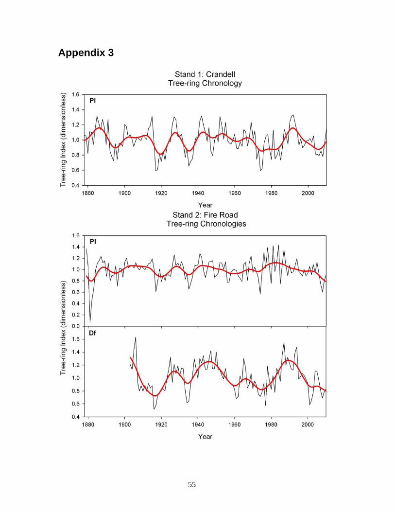
55

Appendix 3

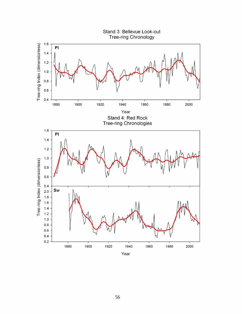
56

57

A3-1. Lodgepole pine and non-host tree-ring chronologies (black line) plotted with a 15-year spline (red line) for each stand.

58

59

60

61

62

63

64

65

A3- 2. Lodgepole pine chronologies from east slopes of the Foothills graphed from north to south (refer to Fig. 1). Black line is tree-ring index and red line is a 15-yr spline.

MPBEP_2011_04_Rpt_EcologicalImpactsoftheMPBonPineForestsoftheSouthernFoothillsAB

Documents

field methods

victoria bc

data analysis

laboratory methods

dendroecological analysis

pacific forestry centre

canadian forest service

data storage