i MOTION PLANNING AND CONSTRAINT EXPLORATION FOR ROBOTIC SURGERY By Sam Bhattacharyya Thesis Submitted to the Faculty of the Graduate School of Vanderbilt University in partial fulfillment of the requirements for the degree of MASTER OF SCIENCE In Mechanical Engineering December 2011 Nashville, Tennessee Approved: Professor Nabil Simaan Professor Nilanjan Sarkar

Welcome message from author
This document is posted to help you gain knowledge. Please leave a comment to let me know what you think about it! Share it to your friends and learn new things together.
Transcript

i
MOTION PLANNING AND CONSTRAINT EXPLORATION FOR ROBOTIC
SURGERY
By
Sam Bhattacharyya
Thesis
Submitted to the Faculty of the
Graduate School of Vanderbilt University
in partial fulfillment of the requirements
for the degree of
MASTER OF SCIENCE
In
Mechanical Engineering
December 2011
Nashville, Tennessee
Approved:
Professor Nabil Simaan
Professor Nilanjan Sarkar

ii
ACKNOWLEDGEMENTS
This work would not have been possible without the financial support of the NSF,
and the Vanderbilt Department of Mechanical Engineering. I would also like to thank my
lab-mates, classmates, the department staff, my professors, my thesis committee, 5 hour
energy™ and of course my advisor Professor Nabil Simaan. G(tb)2.

iii
TABLE OF CONTENTS
Page
ACKNOWLEDGEMENTS ........................................................................................... ii
NOMENCLATURE ........................................................................................................v
LIST OF FIGURES ...................................................................................................... vi
LIST OF TABLES ....................................................................................................... viii
Chapter
I. INTRODUCTION ................................................................................................8
A. Motivation ......................................................................................................8
B. Scope and Problem Statement ........................................................................9
C. Related Laboratory Work .............................................................................12
D. Contributions and Outline ............................................................................12
II. LITERATURE REVIEW ..................................................................................14
A. Constraint Identification ...............................................................................14
B. Exploration of Unknown environments .......................................................17
C. Path Planning in Flexible Environments ......................................................19
III. MATHEMATICAL BACKGROUND ..............................................................21
A. Mechanics/Analytical Methods ....................................................................21
i. Screw Theory ...................................................................................21
ii. Mechanical Constraints ....................................................................23
iii. Spatial Stiffness in the context of Screw theory ..............................27
B. Numerical Methods ......................................................................................30
i. Numerical Optimization ...................................................................30
ii. Clustering .........................................................................................33
iv
iii. Stochastic Methods ..........................................................................35
IV. PATH PLANNING FOR SAFE MANIPULATION .........................................41
A. Function Definition ......................................................................................42
B. Algorithm Augmentation .............................................................................47
C. Safe Manipulation Algorithm .......................................................................51
D. Simulation ....................................................................................................52
E. Results ..........................................................................................................57
V. CONSTRAINT DETECTION, CLASSIFICATION AND MAPPING ............60
A. Spatial Stiffness ............................................................................................61
B. Stiffness Regions ..........................................................................................62
C. Elementary Constraints ................................................................................64
D. Constraint Identification and Classification .................................................67
E. Constraint Exploration Algorithm ................................................................68
F. Experimental Evaluation ..............................................................................69
G. Discussion ....................................................................................................76
VI. CONCLUSION ..................................................................................................79
BIBLIOGRAPHY .........................................................................................................81
APPENDIX A (Code) ....................................................................................................86
APPENDIX B (Code) ..................................................................................................122

v
NOMENCLATURE
Table 1: A list of symbols and nomenclature used in this publication
Symbol Description
7 Dimensional gripper position/orientation in space
3-dimensional Cartesian position
4-dimensional quaternion orientation
6 – dimensional twist vector in Cartesian space
Elastic reaction Wrench, exerted on the environment by the gripper
Local Stiffness Matrix
E Elastic energy exerted on the elastic system by the gripper
Designation for Mechanical Constraint
Constraint Vector
Path Planner Optimization function
Diagonal Dimensional weighting matrix
Designation for Stiffness Region
Axis coordinate conversion matrix
Screw pitch
Eigenvalue
Principle Rotational Stiffness
Principle Translational Stiffness
Dimensional weighting factor

vi
LIST OF FIGURES
Page
1. Semi rigid object suspended in a flexible environment 10
2. Unknown Environment 10
3. Theoretical Reconstruction of the unknown environment 11
4. General Rigid Body Motion 23
5. Planar Constraint 24
6. Pin Joint Constraint 25
7. Peg-in-hole Constraint 26
8. Ball Joint Constraint 26
9. Spatial Stiffness Model 27
10. Steepest Descent Algorithm 31
11. Non-Linear Optimization Algorithm 32
12. Illustration of Clustering 33
13. State Machine 36
14. Markov Chain 36
15. Backtrack Algorithm 49
16. Safe Manipulation Algorithm 51
17. Rigid Triangle 57
18. Safe Manipulation Setup 58
19. Autonomous Navigation: Wrench Profile 58
20. Autonomous Navigation: Pose Profile 59
21. Stiffness Region Example 62
22. Frame Invariant Constraint: Normal Vectors on a curved surface 65
23. Real Membrane Constraint 65
24. Constraint Exploration Algorithm 69
25. Constraint Identification Experimental Mock-Ups 70
26. Constraint Identification using clustering 72
27. Foam Membrane Experimental Setup 73
28. Constraint Detection using clustering, Foam Sheet 74
vii
29. Constraint Map, with Stiffness regions, of a Foam sheet 75
30. Foam Sheet Mock-Up 76
31. Planar Robot Simulation 52
32. Planar Robot Simulation, Feasibly Goal 53
33. Error Profile, Feasible Goal 54
34. Wrench Profile, Feasible Goal 54
35. Planar Robot Simulation, Infeasible goal 55
36. Error Profile, Infeasible goal 56
37. Wrench Profile, Infeasible goal 56
38. Planar Simulation of Object manipulation 41
39. Biomechanical Tissue Properties 77

viii
LIST OF TABLES
Page
1. Nomenclature 5
2. Translational Constraint Vectors from Local Stiffness 73
1
CHAPTER I
I INTRODUCTION
I.A Motivation
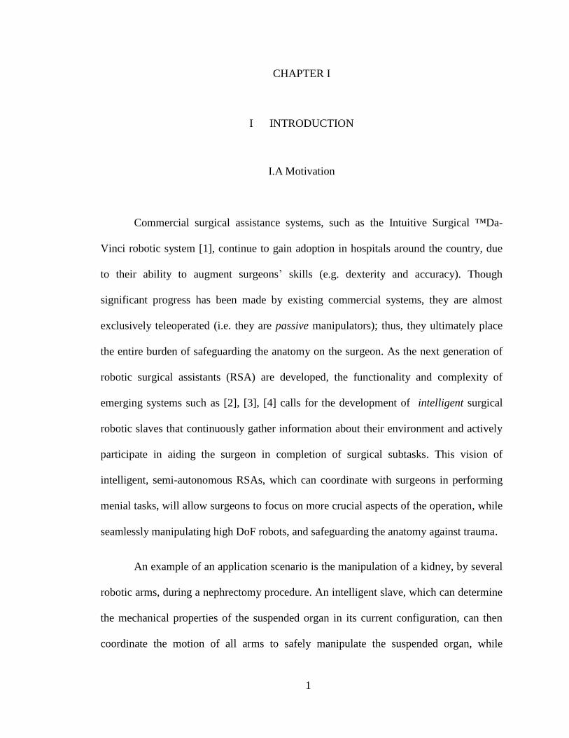
Commercial surgical assistance systems, such as the Intuitive Surgical ™Da-
Vinci robotic system [1], continue to gain adoption in hospitals around the country, due
to their ability to augment surgeons’ skills (e.g. dexterity and accuracy). Though
significant progress has been made by existing commercial systems, they are almost
exclusively teleoperated (i.e. they are passive manipulators); thus, they ultimately place
the entire burden of safeguarding the anatomy on the surgeon. As the next generation of
robotic surgical assistants (RSA) are developed, the functionality and complexity of
emerging systems such as [2], [3], [4] calls for the development of intelligent surgical
robotic slaves that continuously gather information about their environment and actively
participate in aiding the surgeon in completion of surgical subtasks. This vision of
intelligent, semi-autonomous RSAs, which can coordinate with surgeons in performing
menial tasks, will allow surgeons to focus on more crucial aspects of the operation, while
seamlessly manipulating high DoF robots, and safeguarding the anatomy against trauma.
An example of an application scenario is the manipulation of a kidney, by several
robotic arms, during a nephrectomy procedure. An intelligent slave, which can determine
the mechanical properties of the suspended organ in its current configuration, can then
coordinate the motion of all arms to safely manipulate the suspended organ, while

2
allowing the surgeon to command movement of one arm or specify target retraction
distance from the surgical site. Another application would the manipulation of organs
within the abdominal cavity, in order to gain access to underlying tissues. A cooperative
intelligent RSA would be able to determine the mechanical properties of the obstructive
organ, and automatically move it in order to increase visibility of/open up access to the
critical underlying tissue.
This aim of this work is three fold: To propose a framework for modeling and
characterizing the mechanical properties of an unknown elastic system, to propose
algorithms for safe autonomous manipulation of tissues in an unknown environment and
finally to propose a methodology for detecting and identifying mechanical constraints of
an arbitrary unknown elastic system. Used in tandem, these tools can enable an intelligent
RSA to autonomously perform surgical subtasks without a priori knowledge of the
workspace, while simultaneously mapping the elastic properties of the environment.
I.B Problem Statement and Scope
For the purposes of this work, we consider a standard 6 degree of freedom (DoF)
manipulator, with an attached robotic gripper, operating in an unknown and flexible
environment. The robot operates in a full 6-dimensional Cartesian workspace, and is
grabbing some semi-rigid object, which is suspended within an elastic environment, as
shown in the figure below. Our definition of semi-rigid is such that, though the object
internal deformation of the object is noticeable smaller than its elastic connections to the
environment. Actual magnitudes will vary with the application, and the environment.
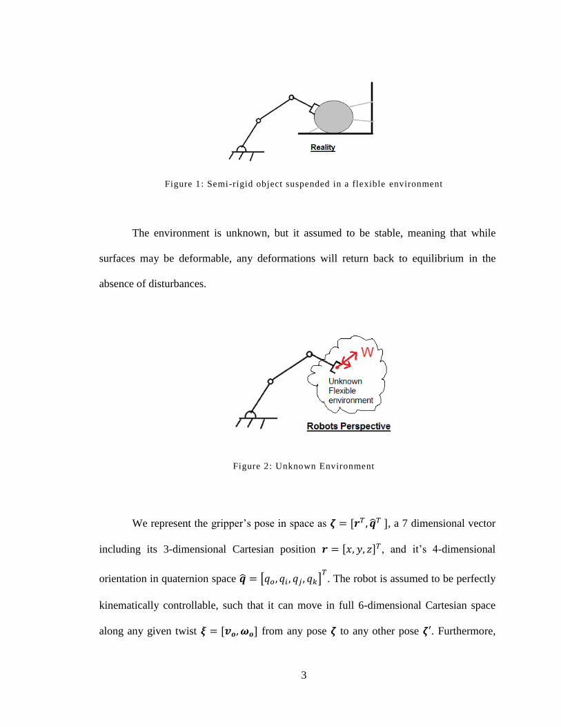
3
Figure 1: Semi-rigid object suspended in a flexible environment
The environment is unknown, but it assumed to be stable, meaning that while
surfaces may be deformable, any deformations will return back to equilibrium in the
absence of disturbances.
Figure 2: Unknown Environment
We represent the gripper’s pose in space as , a 7 dimensional vector
including its 3-dimensional Cartesian position , and it’s 4-dimensional
orientation in quaternion space [ ] . The robot is assumed to be perfectly
kinematically controllable, such that it can move in full 6-dimensional Cartesian space
along any given twist from any pose to any other pose . Furthermore,

4
the robot is equipped with 6-axis force sensing capability, and can measure the elastic
wrench acting on the robot by the environment. In this work, we are not considering
any forces due to gravity, dynamics or friction, as the former two can easily be
compensated for in practice, while the latter is kept out of the scope of this work, since
models of internal organ friction are not available yet. .
The problem to be solved, therefore, can be stated as such: Given the initial
object pose , manipulate the object to a new pose , while avoiding exceeding a
critical force at any point, on the unknown elastic system, and while minimizing the
elastic energy exerted on the elastic system.
This Thesis will present a solution to the aforementioned problem, and also
answer the following 5 problems: 1) Develop a model to describe the elastic properties of
the environment, 2) use to identify the mechanical constraints of the system, 3) Use
information to intelligently navigate the workspace, 4) Create a map of these constraints
throughout the workspace and 5) Use the information to aid in future manipulation tasks
and goals. These problems will be sequentially solved in chapter IV and V of this thesis.
Figure 3: Theoretical Re-construction of the unknown environment
5
In order to develop a proper solution, a very basic assumption is made about the
elastic system. Firstly, a maximum safe elastic energy/elastic force is assumed, below
which exertion of such force or elastic energy will not damage the environment. The
range and scales of such values will be application dependent, and while this does
constitute a-priori knowledge about the environment, information of this kind of can be
easily obtained through bio-mechanics references for tasks in the surgical domain.
I.C Related Laboratory Work
The work presented in this thesis was done at the ARMA lab at Vanderbilt
University, under the direction of Dr. Nabil Simaan. This work ties into the work done
by current and former students of the lab, who have worked in the areas of local stiffness
exploration, contact and constraint detection for surgical robots. In [15], Xu and Simaan
(2009) implement stiffness mapping of the surface of an organ, using the intrinsic force
sensing capabilities of a snake-like RSA. In [36], [37], Goldman et al. (2010, 2011) use
the same RSA for exploration of shape and local impedance of an unknown
environment. Finally, in [47] Bajo et al. (2011) presented work on detection of contact
for the same snake-like RSA.
I.D Contribution and outline
The primary contributions of this work are in validating the feasibility of
autonomous manipulation in an unknown elastic environment, in developing a real-time

6
compatible representation of global stiffness properties, and in presenting methods for
automatically identifying and classifying flexible constraints in real time.
Previous works on exploration mainly focus on constraint exploration in rigid
environments (Lefebvre) [44], constraint identification of tools (Dupont and Howe) [9],
and exploration in rigid environments (Okamura and Kutcowsky) [11]. To date, there are
no clear frameworks to exploration in flexible environments. A recent exception is the
work of Goldman in [36], [37] where exploration of shape, and local impedance has been
carried out. This work extends these results to include the characterization of organ
constraints and path planning for safe manipulation.
First, in section II, works in the related areas of path planning and environment
exploration are reviewed in detail. In section III, some necessary background, including
Spatial Stiffness theory and AI methods, are reviewed. An algorithm for blind, safe,
autonomous manipulation is proposed in section IV, and then experimentally validated
using a Puma 560 industrial robot arm. Finally, section V details our methods for
characterizing, identifying and mapping the elastic constraints of a workspace in real
time, and presents experimental evaluation of these techniques on real flexible objects
using the Puma 560.

7
CHAPTER II
II LITERATURE REVIEW
There have been numerous works on the relevant topics of environmental
exploration, detection of contact, constraint identification and path planning in elastic
environments. The solutions presented in these works operate in restricted domains
however, and only provide solutions to parts of the problem posed in the previous
section.
II.A Constraint detection/identification
He [5,6] explicitly dealt with the exploration and detection of mechanical
constraints (“Contact States”) between two rigid objects. Xiao developed a simple model
of a manipulator grasping a movable polyhedron A, which is possibly in contact with
fixed polyhedron B, and represented the contact as the super-position as a combination of
“principle contacts”, simple dimensionless/directionless kinematic constraints. He then
assumed that the geometry (shape, dimensions and position/orientation) of the objects
was known, but with experimental uncertainty. Xiao simply defines a method for
resolving the rigid kinematic model with the actual experimental data, to determine the
most likely contact state for a given configuration of object A. This methodology works,
however it requires explicit geometric information about the object being manipulated,
8
especially since it works entirely in the kinematic domain (constraints are not considered
as reaction forces, but rather as purely kinematic constraints).
De Schutter [7] also deals with manipulation of objects with known geometries
and an appropriate kinematic map (with experimental error), but tackles the problem of
constraint identification, for manipulation under flexible constraints. To do this, he
represents the flexible constraint of an object at a given configuration as a virtual
compliant manipulator. This virtual manipulator results in the same degrees of freedom
as the object, but models the compliance in each direction of motion, to provide
predictions in the changes of the constraint forces as the real manipulator moves in space.
This methodology allows for simple characterization/representation of elastic constraints
in a given workspace, however it requires explicit kinematic models of the environment
and assumes known geometries ahead of time.
Kitagaki and Suehiro [8] get rid of the assumption of known geometric/kinematic
models by incorporating force information. Assuming a manipulator with an attached
force sensor, manipulating an object in a rigid environment, they estimate the location of
point contact using static balancing. The associated constraint results in a normal force,
which will result in an applied moment on the force sensor. Furthermore, they present
models for detecting edge on plane constraints, and propose methods detection of contact
state transitions. This methodology is powerful and simple, however it assumes a rigid
environment, and furthermore requires high accuracy force measurements of contacts
with very high rigidity.

9
Dupont [9] presented a simple but effective method for modeling and identifying
kinematic constraints of a general robotic manipulator. He does this by using the notion
that, for a kinematic constraint, no constraint wrench can do any work about a freedom
twist (see section III.A.2). He suggests that for a manipulator’s end effector, at a certain
position while moving along a trajectory, any forces/torques in the direction of the
trajectory cannot be due to a constraint force, and furthermore, that any forces/torques
normal to the trajectory are due to a kinematic constraint at that location. Correcting for
dynamics and gravity forces at the end effector, he then utilizes this method to
automatically explore the kinematic constraints on surgical instruments during insertion.
Howe [10] uses probabilistic methods to infer contact and constraint properties of
a given object being manipulated, using experimental force/position data. He assumes a
set of known Kinematic constraints (“Contact States”), and develops geometric models
for each of these constraints, which are independent of size/scale/orientation. For a given
robot manipulation task, force/kinematic data are then simultaneously evaluated on how
well it matches each geometric model. A hidden Markov model is then used to
stochastically determine the current contact state, using a closest fit to that contact state’s
model.
To the author’s knowledge, none of these works deals explicitly with
identification of flexible constraints in unknown environments, with the exception of
course being Goldman (2011). With high-DoF RSAs further abstracting the interface
between the surgeon and the patient anatomy, there is a clear need for further
investigation in this area to enable proper force feedback and semi-autonomous
manipulation schemes in robotic surgery.
10
II.B Exploration of unknown environments
Okamura and Cutkosky [11, 12] focus on the haptic exploration of objects using
robot fingers which are equipped with tactile sensors. They use feature based exploration
to map and characterize the surface properties of an object being grasped by a robotic
hand. They define classes of features, macrofeatures, such as a ‘bump’ feature, or a
‘ridge’ feature, and present methods for detecting instances on these macrofeatures on an
object being grasped. A map of these features on an object represents a tactile signature,
and could then be used to identify/characterize the particular object being grasped.
Allen [13] also worked on haptic exploration of objects using robot fingers,
however he focused on developing models of the geometric shape of the object, rather
than mapping/characterizing the stiffness properties. Allen uses tactile and kinematic
information to define a set of contact points in space, corresponding to where the
fingers/hand is in contact with the object. He then fits these points to a 3-dimensional
superquadric function, to recover the general form of the object in space, from a set of
sparse contact data.
One alternative to representing elasticity as FEM is to use a stiffness map, map
over the workspace which simply measures the magnitude of the stiffness at each
location. Althoefer [14] and Xu[15] [38], both present devices which can be used to
develop stiffness maps over a flexible surface, which can be used to detect specific
features, such as sections of high rigidity, while exploring an elastic workspace. They do
this by simple considering stiffness as the spatial derivative of force, and use the
kinematic models and intrinsic force sensing capabilities of their devices to map the

11
stiffness in a given region. Exploration of stiffness in this manner can be used to detect
features, such as tumor, on an on organ during surgery. Since such stiffness maps only
explicitly consider magnitude, they cannot be used for characterizing mechanical
constraints, which are inherently direction dependent at a given location. These works
explore normal stiffness. Goldman extended these works to include exploration of
perceived impedence tensors (damping, stiffness, inertia).
Finally, Gupta [16] presents a straightforward method for simultaneous path
planning and exploration of an unknown workspace, using a robot manipulator and a
tactile “skin” sensor. Using the sensor, it is assumed that contact can be measured at any
point on the robot manipulator, and Gupta proposes an algorithm for systematically
exploring the unknown workspace, and recording positions without contact as the
“freedom space”. Given sufficient time to explore the workspace, the algorithm will have
developed a full map of the workspace, broken down into the “freedom space” and the
constraint space.
Most of these works, which deal with contact estimation of environment
exploration, assume a rigid and otherwise static environment, which, for many
applications is certainly valid. Despite the progress made in environment exploration,
contact detection and constraint estimation, to the best of our knowledge, little work has
been done on the blind characterization and estimation of flexibly constrained objects in
unknown environments.
12
II.C Path Planning
As opposed to environmental exploration, path planning is a subject which has
had some attention, in the context of flexible/elastic environment. Using a force based
approach and an FEM model, Rodriguez [17] considered the path planning issues of
navigating in a completely deformable known environment. By using a Rapidly-
Exploring Random Tree algorithm and a collision detection algorithm, they attempt to
minimize the elastic energy in all of the possible paths that could be taken to reach the
end goal. They used this path planning method to simulate a robot navigating around
flexible organs/tissues within the human chest cavity.
Patil et al. [18] used finite element methods to model the elastic characteristics of
a flap of tissue being manipulated during organ retraction. Patil uses an offline
optimization algorithm to pre-compute an optimal path for a given manipulator to retract
the tissue in order to maximize the area exposed under the flap, while minimizing the
elastic energy exerted on the tissue.
Gayle et al. [19] model a deformable robot moving through a flexible
environment, and proposes an algorithm which uses a finite element model and virtual
dynamic equations to compute an optimal path (offline) for the robot from a start goal to
a finish goal, while observing a set of hard constraints. They then apply this methodology
to optimize the path for a snake robot which enters the femoral artery (in the legs) and
navigates to the liver to perform some operation.

13
Like Rodriguez and Patil, Gayle assumed a known environment and used FEM to
model its elasticity. There are many other works on path planning methods in flexible
environments, but which almost exclusively deal with Finite element methods and off-
line path planning. While they are effective for providing theoretically optimal paths in a
given scenario, real-time implementation of these paths will never be perfect. Hence there
is great potential in utilizing real time exploration of constraints.
14
CHAPTER III
III MATHEMATICAL BACKGROUND
III.A Stiffness, Compliance and Screw Theory
III.A.1 Screw theory
In Cartesian space, there are 6 dimensions of motion for a general rigid body:
Translation along the three Cartesian axes, and rotation about each of those axes .While
absolute orientation cannot be represented completely in only 3 dimensions, any
Cartesian angular velocity can be expressed completely in 3 dimensions.To represent a
general velocity in space, we can then define a 6 dimensional vector, which includes
three translational velocities, and 3 angular velocities. This vector will be denoted as
[
] (1)
Chasle’s theorem forms the basis for screw theory, and can be stated as such: The
most general displacement for a rigid body in space can be described as translation along
a line in space, and a rotation about that same line. Plucker coordinates can be used to
describe any such line in space, and are composed of 6 homogenous coordinates\
[
] (2)
Where describes the direction of the line, and is a vector from the origin to
any point on the line. These 6 homogenous coordinates can accurately describe any line
in space. Now consider again the general 6-dimensional vector [
]

15
The rotation around a vector (along a general line in space) can be expressed in
plucker coordinates, as follows
[
] (3)
As can be seen, when the line is away from the origin, the rotation about that line
will create a velocity normal to the line. Depending on the direction and magnitude of ,
any velocity normal to can be expressed as . As Chasle’s theorem states, any
general rigid body motion can be described by the movement along a line in space, and
around that line in space. Any velocity that is along the direction of the axis of rotation
can be modeled as a screw such that rotation around the axis is coupled with a translation
along that axis, via pitch h. . If we add this term to the Plucker line
coordinates, we get:
[
] (4)
Since can be used to represent any velocity normal to and can be used to
represent any velocity along , any general velocity can be described at
Thus, we can represent the general motion [
] as a screw vector [
].
If , the twist corresponds to a revolute joint. If , the twist corresponds to a
pure translation.
can be calculated as
( )
|| || (5)
can be calculated as
16
(6)
Using screw theory, it is possible to analyze twist vectors to analyze centers of
rotation and to classify and characterize complex rigid body motions.
It is also possible to analyze force and moments using screw theory. This is done
by considering a general 6-dimensional force/moment
[
] (7)
As done with twists, the moment can be expressed as a perpendicular component
and a parallel component . Thus, any force/moment in space can be expressed
as:
[
] (8)
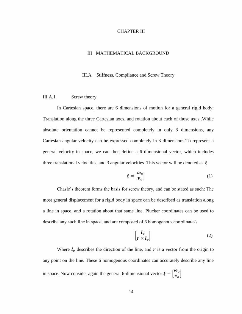
III.A.2 Mechanical Constraints
The concept of mechanical constraints is used to describe kinematic restrictions on
the movement of rigid objects in space. Consider a general 3-dimensional rigid object
suspended in 6-dimensional Cartesian space, as shown in Figure 4 below.
Figure 4: General rigid body motion
17
If there are no constraints on the movement of this object, then it can follow any
general twist in 6-dimensional space (6 Degrees of Freedom), without restriction. For
most practical applications in robotics/engineering, this is usually never the case, as
objects aren’t simply suspended in space. Rather, most objects at rest are constrained
from motion along certain directions, due to gravity, friction and contact with the
environment, and are thus restricted the fewer than 6 degrees of freedom. As an example,
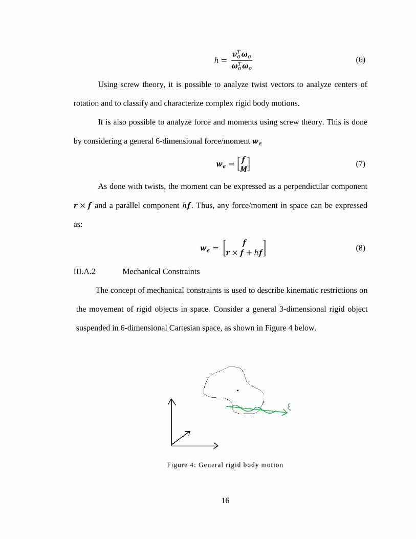
consider a book lying on a table, as shown below:
Figure 5: Planar Constraint
The book is free to slide along the table, and can rotate around the normal axis of
the table. It is, however, restricted from moving into the table, and from rotation around
axes in the plane of the table. Thus, it has been restricted to 3 DoF, by restrictions along 3
directions of motion. This particular form of motion restriction is known as a planar
constraint, which is one of a large set of mechanical constraints. A mechanical constraint
is composed of a set of restrictions on the motion of an object along a set of directions.
The directions along which there is no motion restriction are known as freedom twists ,
since twists along these directions incur no resistance. Directions along which motion is
impeded, due to rigid body contact or friction, are known as constraint wrenches , as
reaction wrenches along these directions prevent rigid objects from moving along them.
18
There are a number of different general rigid body constraints, that are represented by
constraint wrenches and freedom twists. A few are described below:
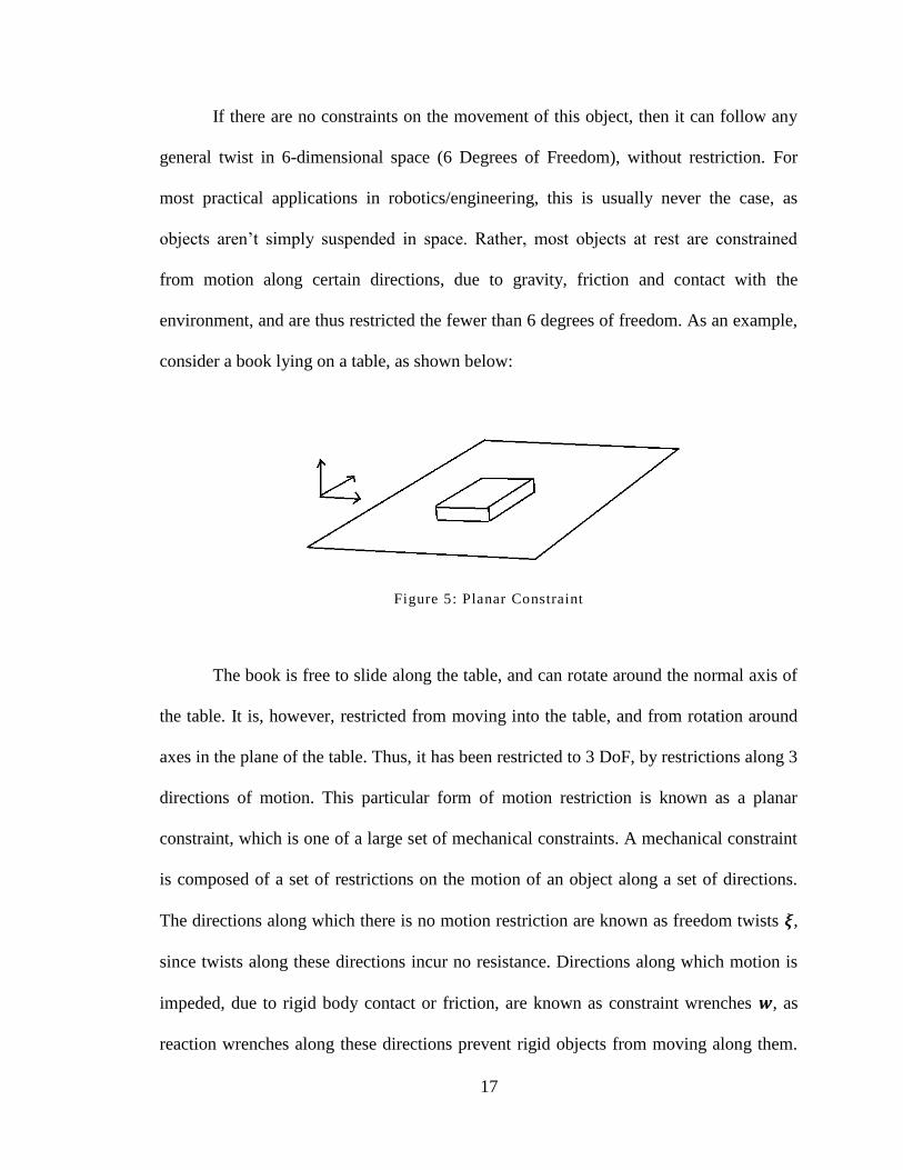
III.A.2.a Pin joint
One of the most common types of constraints is a pin-joint constraint, as shown in
the diagram below. Pin joints contain only one DoF, rotation along an axis. Accordingly,
the joint itself is composed of 5 constraint wrenches, which prevent Cartesian translation
of the joint, as well as rotation around axes which are perpendicular to the primary axis of
rotation.
Figure 6: Pin Joint Constraint
Real examples of pin-joints would include any type of hinge, or a robotic arm.
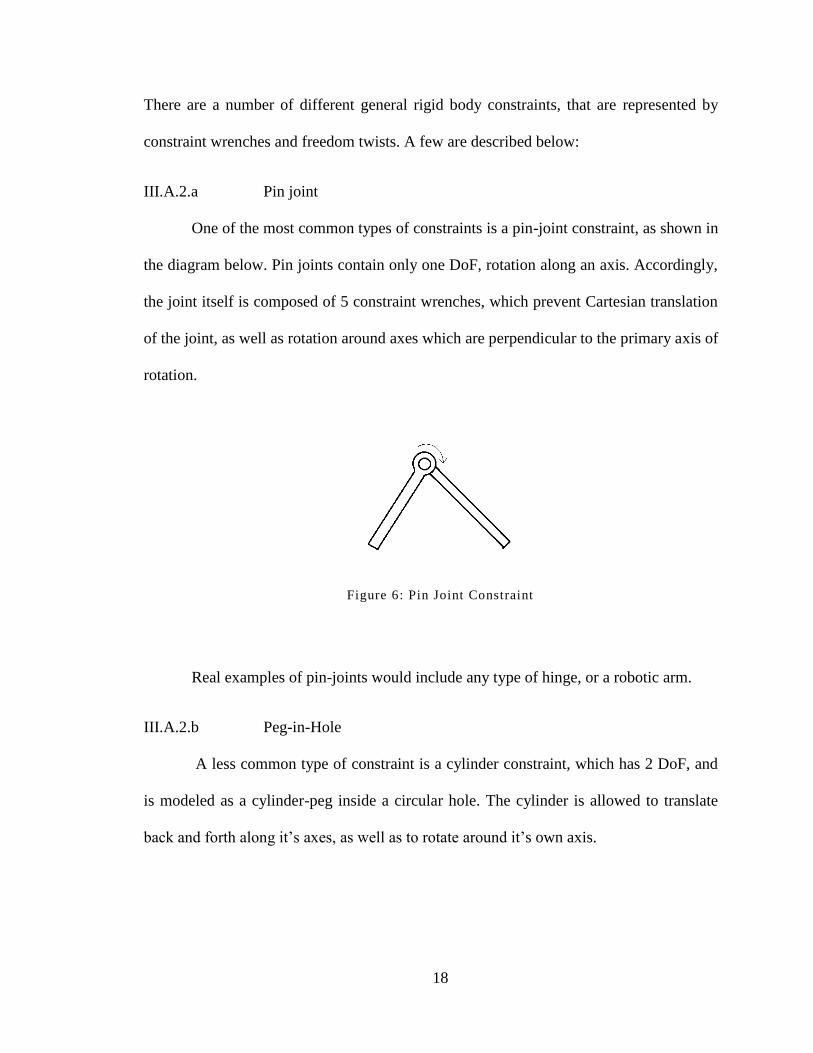
III.A.2.b Peg-in-Hole
A less common type of constraint is a cylinder constraint, which has 2 DoF, and
is modeled as a cylinder-peg inside a circular hole. The cylinder is allowed to translate
back and forth along it’s axes, as well as to rotate around it’s own axis.
19
Figure 7: Peg in hole constraint
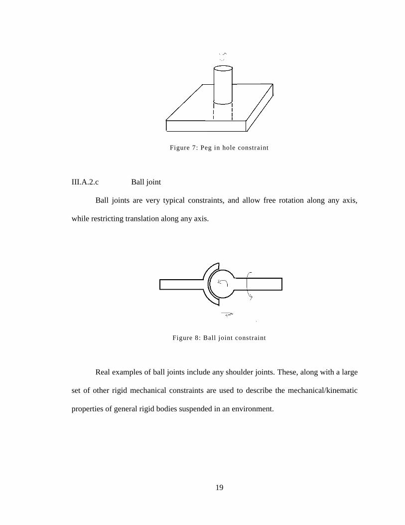
III.A.2.c Ball joint
Ball joints are very typical constraints, and allow free rotation along any axis,
while restricting translation along any axis.
Figure 8: Ball joint constraint
Real examples of ball joints include any shoulder joints. These, along with a large
set of other rigid mechanical constraints are used to describe the mechanical/kinematic
properties of general rigid bodies suspended in an environment.
20
III.A.3 Spatial Stiffness in the context of screw theory
For surgical applications, in which we wish to describe objects suspended in
unknown elastic environments, the rigid mechanical constraint models described above
are no-longer applicable. Fortunately, there has been a great deal of work done in the late
90’s and early 2000’s to analyze spatial stiffness and elastic environments using screw
theory, allowing simpler representations of complex elastic behavior and providing
insight into the fundamental elastic properties of the system.
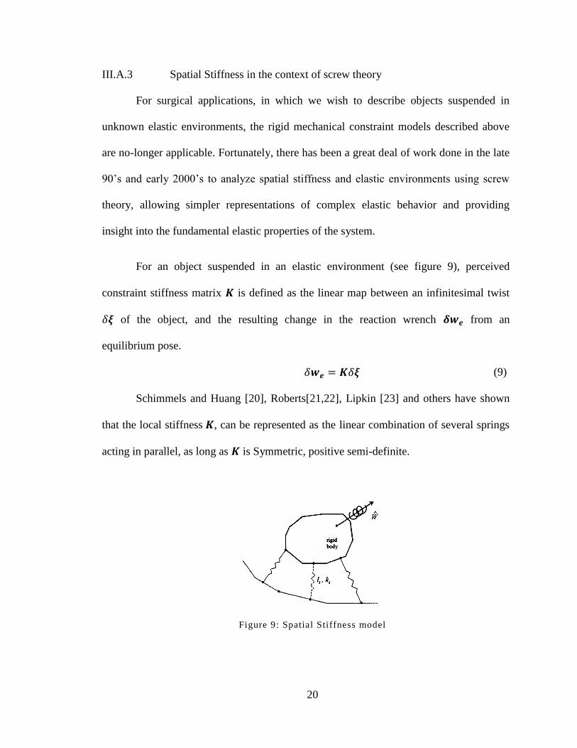
For an object suspended in an elastic environment (see figure 9), perceived
constraint stiffness matrix is defined as the linear map between an infinitesimal twist
of the object, and the resulting change in the reaction wrench from an
equilibrium pose.
(9)
Schimmels and Huang [20], Roberts[21,22], Lipkin [23] and others have shown
that the local stiffness , can be represented as the linear combination of several springs
acting in parallel, as long as is Symmetric, positive semi-definite.
Figure 9: Spatial Stiffness model
21
This is done via matrix decompositions of , and provides a more intuitive
representation of the stiffness than the regular stiffness matrix, as well as some
information about the fundamental properties of the system.
The Eigenvalue problem of (equation 10) is one such decomposition, and
yields 6 eigenvectors and eigenvalues. The system can then be modeled by 6 complex
springs (springs with both linear and torsional components), each with a direction and
magnitude of one of the eigenvectors and its associated eigenvalue respectively.
(10)
Like many other decompositions, this one is not frame-invariant, and will result in
different eigenvectors and eigenvalues, based on the frame being considered. While the
eigenvectors will never be frame independent, both [32] and [33] present modified
eigenvalue problems which will yield frame invariant eigenvalues.
Schimmels proposes the “Eigenscrew Decomposition”, in which the only
modification is a delta matrix [
] and formulates the eigenscrew problem
as in equation (11)
(11)
The effect of the matrix is to interchange the first and last three elements of a 6-
dimensional axis, which converts between axis screw coordinates ( [
]) to ray
screw coordinates [
] , in order to preserve the units. This yields a set of
eigenvalues which are frame invariant, in units of , and as Schimmels argues,
provides insight into the fundamental nature of the problem.
22
Lin [39] breaks into sub-matrices [
], uses matrix algebra
to cancel out frame-dependent components of , resulting in the following sub-matrices
(12)
Where the eigenvalues of are the principle rotational stiffnesses of ,
the eigenvalues of are the principle translational stiffnesses of . The result
is a set of 3 orthogonal, rotational axes and set of 3 orthogonal translational axes, whose
magnitudes are frame invariant and describe the pure rotational and pure translational
behavior of the system.
Lipkin [25] uses a similar analysis to define the principle rotational stiffness axes
and the principle translational compliant axes of a stiffness matrix , and then uses them
to create rotational and translational elasticity ellipsoids.
The tools outlined above can and will be used to analyze the mechanical
properties of unknown elastic environments. As Schimmels et al. discuss [24], any proper
eigenvalue or eigenscrew decomposition requires a Symmetric, positive, Semi-Definite
(SPSD) matrix, which is almost never obtainable from experimental numbers (due to
noise and displacement from equilibrium). Thus, in order to experimentally implement
this analysis, an SPSD matrix needs to be derived from experimentally gathered data.
Ellis and McAllister [26] present a method of doing so, by using an SPSD approximate
of a given experimentally derived stiffness matrix . The solution is explained in
[27] and is summarized below:
(13)
Take the Eigenvalue decomposition of B
23
(14)
Where is a matrix of eigenvectors and is a diagonal matrix of eigenvalues.
| | (15)
(16)
The result is a close approximate of the stiffness matrix , which will not include
negative or complex eigenvalues.
III.B Numerical Optimization and Stochastic Methods
The previous chapter presented an entirely analytical framework for describing
and understanding flexibility and spatial stiffness using screw theory. When the necessary
information is available, and the analytical models are applicable, analytical methods are
effective, efficient and provide broader insight into the structure of the problem.
In real world applications such as robotic surgery however, complete information
almost never available. In order for an autonomous Robotic Surgical Assistant to operate
is any such environment, it has to explore, gather data, and make intelligent decisions
using incomplete information, without compromising the safety of the patient. To tackle
these problems, a variety of numerical, computational and AI methods can be used. This
chapter will discuss the ideas of Numerical Optimization, Clustering, Markov models,
Particle Filtering and Monte-Carlo methods.
III.B.1 Numerical Optimization
Consider some function ( ), which is a function of many variables for which
computation of ( ) is easy, while the inverse ( ) is highly intractable.
24
The problem of optimization (finding the which will minimize/maximize ) usually
cannot be solved analytically, even though evaluating the function is trivial. For this
situation, numerical methods can be utilized to navigate the domain space , and
find the vector of inputs which will locally or globally minimize ( )
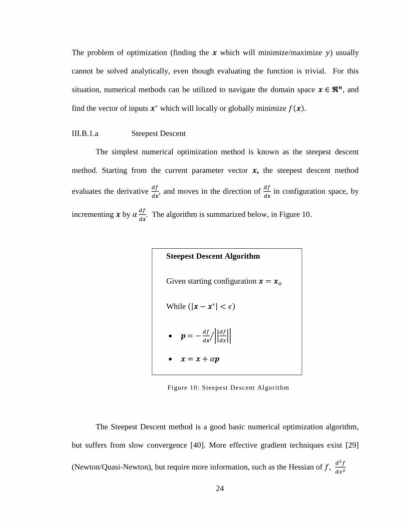
III.B.1.a Steepest Descent
The simplest numerical optimization method is known as the steepest descent
method. Starting from the current parameter vector , the steepest descent method
evaluates the derivative
, and moves in the direction of
in configuration space, by
incrementing by
. The algorithm is summarized below, in Figure 10.
The Steepest Descent method is a good basic numerical optimization algorithm,
but suffers from slow convergence [40]. More effective gradient techniques exist [29]
(Newton/Quasi-Newton), but require more information, such as the Hessian of ,
Steepest Descent Algorithm
Given starting configuration 𝒙 𝒙𝑜
While (|𝒙 𝒙 | < 𝜖)
𝒑 𝑑𝑓
𝑑𝒙 𝑑𝑓
𝑑𝑥
𝒙 𝒙 𝛼𝒑
Figure 10: Steepest Descent Algorithm

25
III.B.1.b Non-Linear Optimization
One such hessian based algorithm is the typical non-linear optimization function.
For example, consider a non-linear system ( ) , where represents the hidden inputs to
the system. Suppose we can observe the output of the system ( ) , and we want to
use the observed variable to learn the hidden variables such that ( ) . To do
this, we define a lease square’s function ( ), as shown in equation 17
( | ( ) | ) ( ) (17)
The non-linear algorithm shown below can be used to find the value of
Figure 11: Iterative Non-Linear least square’s Optimization algorithm
Iterative Non-Linear Least Square’s Solver
Given y
Make initial guess for 𝑛 1 vector 𝒙𝑖
Error vector 𝒆 𝒇(𝒙𝑜) 𝒚
𝑤 𝑖𝑙𝑒
𝒆𝑇𝒆 < 𝜖
o 𝒃 𝒃 𝒇(𝒙)
o 𝐴 𝜕𝒇
𝜕𝒙
o Δ𝒙 𝐴 𝑇𝐴
𝐴 𝑇𝒃
o 𝒙 𝒙 Δ𝒙
o 𝒆 𝒇(𝒙) 𝒚
End
26
One advantage to this algorithm versus the steepest descent, is the ability to stack
multiple observations [
] and dynamically update the estimates as new
observations are made.
III.B.2 Clustering
For any kind autonomous RSA to operate intelligently, it needs to gather data
from the environment, subsequently make inferences and conclusions from sparse and
possibly incomplete data. Instead of pre-defining theoretical models to classify data
based on how it ‘should’ fit (i.e., this stiffness matrix should represent a planar
constraint, based on our geometric model), there are a number of statistical methods
available for recognizing patterns and classifying data automatically [30], including
Principle Component Analysis (PCA) and Bayesian Networks. In this work however, we
focus on Clustering.
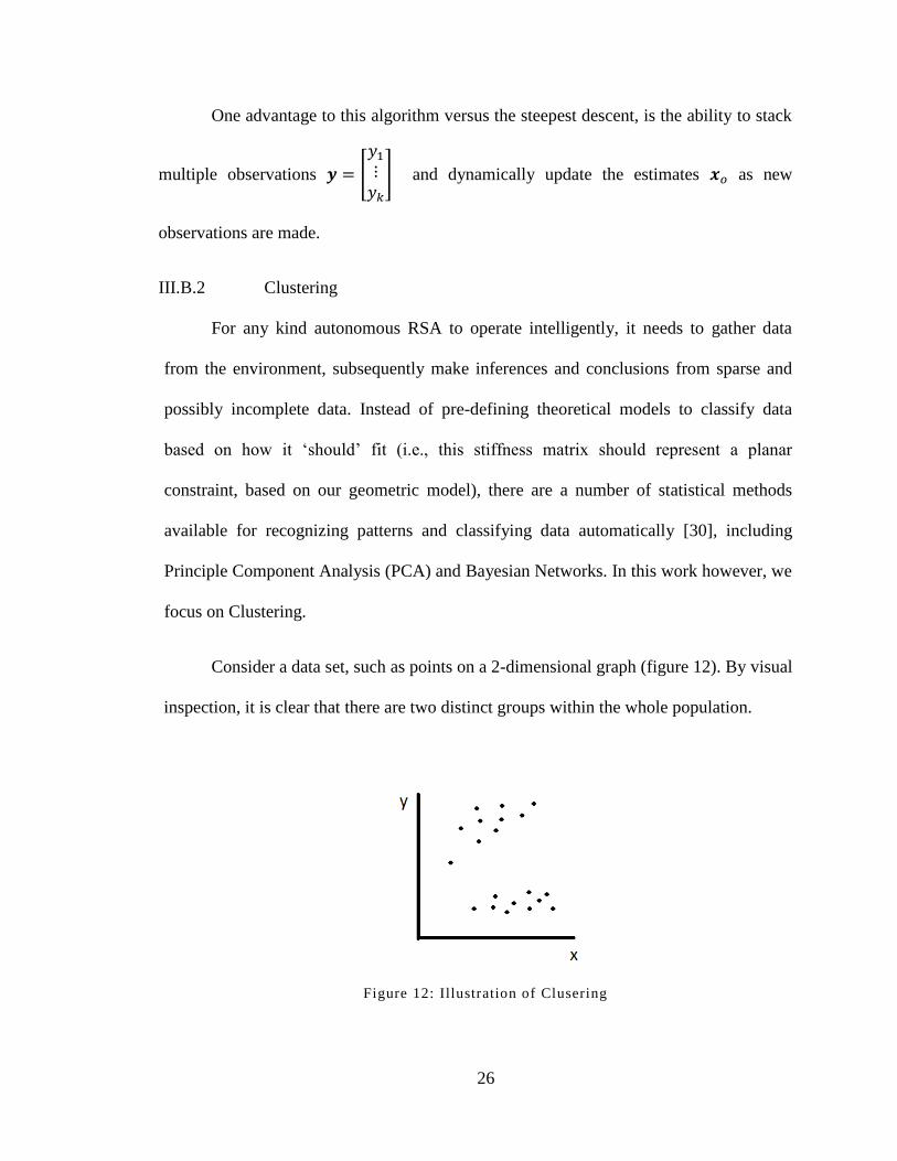
Consider a data set, such as points on a 2-dimensional graph (figure 12). By visual
inspection, it is clear that there are two distinct groups within the whole population.
Figure 12: Illustration of Clusering
27
In the language of clustering, each individual point/measurement is called an
‘Example’ , and each example has a feature vector (x and y values) with
elements ( in this case). In hard clustering, we wish to organize and classify
this data set into groups called classes (ideally 2 groups in this case) which share
similar feature vectors.
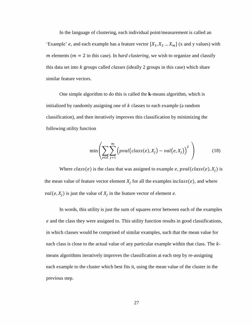
One simple algorithm to do this is called the k-means algorithm, which is
initialized by randomly assigning one of classes to each example (a random
classification), and then iteratively improves this classification by minimizing the
following utility function
(∑ ∑ ( )
) (18)
Where ( ) is the class that was assigned to example , ( ( ) ) is
the mean value of feature vector element for all the examples in ( ), and where
( ) is just the value of in the feature vector of element .
In words, this utility is just the sum of squares error between each of the examples
and the class they were assigned to. This utility function results in good classifications,
in which classes would be comprised of similar examples, such that the mean value for
each class is close to the actual value of any particular example within that class. The -
means algorithms iteratively improves the classification at each step by re-assigning
each example to the cluster which best fits it, using the mean value of the cluster in the
previous step.

28
Eventually, the -means algorithm will reach a stable classification (a local
minimum of the utility function), which can be used to making decisions / inferences /
predictions about current and new data points. This simplified algorithm is only a local
optimizer, and is not guaranteed to find the optimal classification of the data set (the
global minimum of ). With data points, and possible classes, there are
possible classifications, the optimal classification problem is exponential in its run time.
Furthermore, the optimal classification problem can be shown to be NP complete, as the
CNF Satisfiability problem (a known NP-complete problem) can be reduced to an
instance of this problem.
III.B.3 Stochastic methods
In the absence of a structured model of a system, such as a clearly defined ( ) or
set of continuous variables , non-derivative based stochastic methods can be used to
model/describe/predict the behavior of complex systems.
III.B.3.a Markov Models
Consider an abstract mathematical model of a system, in which the system can be
in one of a finite number of states at any given time. This is called a state machine, and it
describes the transition of the system from one state to another. They system could be as
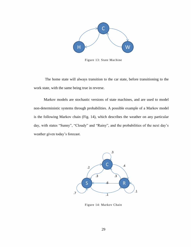
simple as a daily commute (see Fig. 13), in which the states are “At Home” (H), “In the
Car” (C), and “At Work” (W).
29
Figure 13: State Machine
The home state will always transition to the car state, before transitioning to the
work state, with the same being true in reverse.
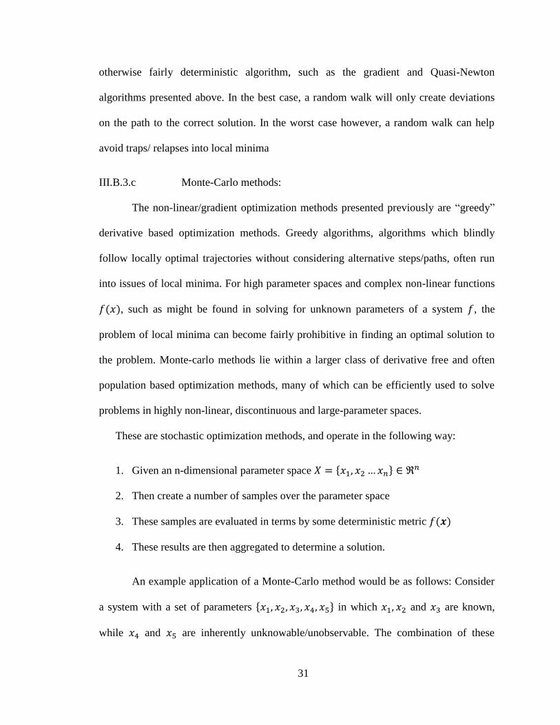
Markov models are stochastic versions of state machines, and are used to model
non-deterministic systems through probabilities. A possible example of a Markov model
is the following Markov chain (Fig. 14), which describes the weather on any particular
day, with states “Sunny”, “Cloudy” and “Rainy”, and the probabilities of the next day’s
weather given today’s forecast.
Figure 14: Markov Chain

30
Using experience from previous weather patterns (specifically, via a state
transition matrix), it is possible to determine the probabilities of these state transitions,
and predict future weather patterns, or infer previous weather patterns, given the current
state.
One example of the use of Markov Models can be seen in Rosen et al (2006) [40],
in which a generalized minimally invasive surgical procedure was broken down into a set
of discrete, elementary subtasks (such as clamping, gripping, etc..). These sub-tasks were
then represented as states in a Hidden Markov model (HMM), and each state was
associated with a certain end effector motion/force profile. Given a set of training data,
the HMM could then be used to guess the current surgical subtask being performed by a
surgeon, by stochastically estimating the current state of the Markov model. Another
example of Markov chains would be the Random Walk algorithm, as discussed below.
III.B.3.b Random Walk
Like a Markov model, random walks are stochastic models that are often used to
describe systems. In the context of Numerical optimization, random walks can be used as
a method of escaping local minima. Given an n-dimensional space, with a state
{ } , a random walk is simply a sequence of random steps in n-
dimensional space, from the current state to some new state.
∑ ( )
(19)
( ) ( ) (20)
( ) here is random uniform distribution from to . Random walks can be
used not only to escape local-minima, but to add a level of non-determinism into an
31
otherwise fairly deterministic algorithm, such as the gradient and Quasi-Newton
algorithms presented above. In the best case, a random walk will only create deviations
on the path to the correct solution. In the worst case however, a random walk can help
avoid traps/ relapses into local minima
III.B.3.c Monte-Carlo methods:
The non-linear/gradient optimization methods presented previously are “greedy”
derivative based optimization methods. Greedy algorithms, algorithms which blindly
follow locally optimal trajectories without considering alternative steps/paths, often run
into issues of local minima. For high parameter spaces and complex non-linear functions
( ), such as might be found in solving for unknown parameters of a system , the
problem of local minima can become fairly prohibitive in finding an optimal solution to
the problem. Monte-carlo methods lie within a larger class of derivative free and often
population based optimization methods, many of which can be efficiently used to solve
problems in highly non-linear, discontinuous and large-parameter spaces.
These are stochastic optimization methods, and operate in the following way:
1. Given an n-dimensional parameter space { }
2. Then create a number of samples over the parameter space
3. These samples are evaluated in terms by some deterministic metric ( )
4. These results are then aggregated to determine a solution.
An example application of a Monte-Carlo method would be as follows: Consider
a system with a set of parameters { } in which and are known,
while and are inherently unknowable/unobservable. The combination of these
32
parameters can deterministically yield one of two implications: and . A Monte-carlo
method could be used to search the parameter space of by creating a set of samples
of these parameters. Each sample of or can be evaluated by their likelihood of
being the value of . The aggregate can then be used to evaluate the probability of or
, given unknown values of and ..The complexity of such problems are
exponential with the number of unknowns , such that given domain size , the run-time
scales with . While Monte-Carlo methods can help stochastically explore a large
domain, it requires prohibitively higher (exponential) number of sample points as the
dimensionality of the problem increases.
III.B.3.d Particle Filtering
Other stochastic population methods, such as Genetic Algorithms and Simulated
annealing, perform an optimization to find optimal configurations of . Particle filtering
is a simple and easy to implement stochastic optimization methods. The algorithm
proceeds as follows:
1. Create a large set of m samples of an n-space, called ‘particles’
2. Assign them random values in the n-dimensional space
3. These particles are assigned some fitness metric
4. These fitness metrics should be weighted to a probability (0-1) such that, the
higher the metric, the higher the probability
5. This will be the probability that this particle will not be eliminated after ‘filtering’
6. ‘filtering’ selects each particle and may delete it, based on its probability
7. New particles are added to the population and the process is repeated
33
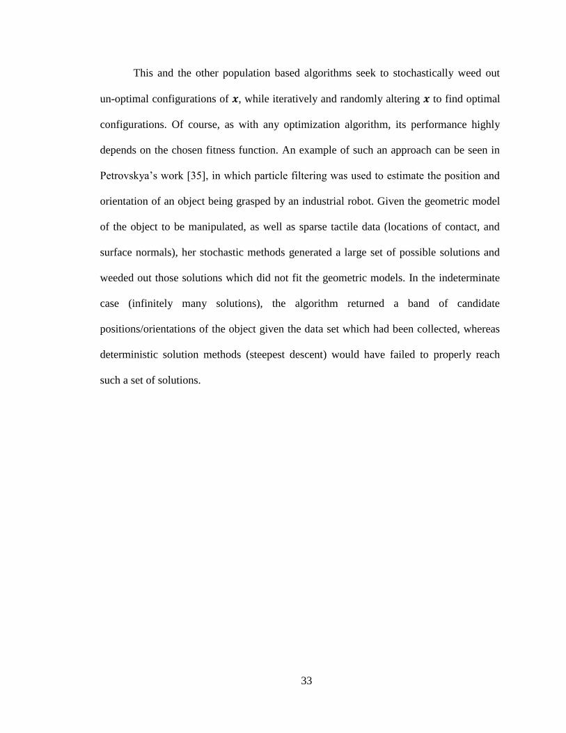
This and the other population based algorithms seek to stochastically weed out
un-optimal configurations of , while iteratively and randomly altering to find optimal
configurations. Of course, as with any optimization algorithm, its performance highly
depends on the chosen fitness function. An example of such an approach can be seen in
Petrovskya’s work [35], in which particle filtering was used to estimate the position and
orientation of an object being grasped by an industrial robot. Given the geometric model
of the object to be manipulated, as well as sparse tactile data (locations of contact, and
surface normals), her stochastic methods generated a large set of possible solutions and
weeded out those solutions which did not fit the geometric models. In the indeterminate
case (infinitely many solutions), the algorithm returned a band of candidate
positions/orientations of the object given the data set which had been collected, whereas
deterministic solution methods (steepest descent) would have failed to properly reach
such a set of solutions.
34
CHAPTER IV
IV PATH PLANNING FOR SAFE MANIPULATION
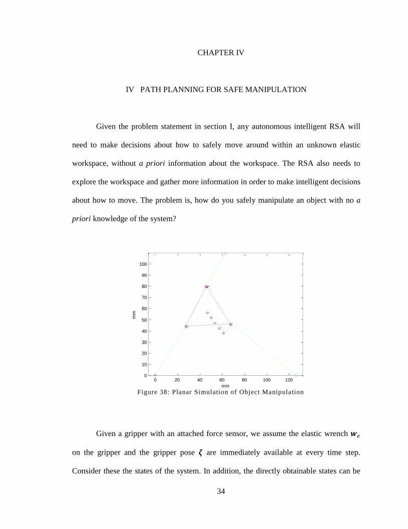
Given the problem statement in section I, any autonomous intelligent RSA will
need to make decisions about how to safely move around within an unknown elastic
workspace, without a priori information about the workspace. The RSA also needs to
explore the workspace and gather more information in order to make intelligent decisions
about how to move. The problem is, how do you safely manipulate an object with no a
priori knowledge of the system?
Figure 38: Planar Simulation of Object Manipulation
Given a gripper with an attached force sensor, we assume the elastic wrench
on the gripper and the gripper pose are immediately available at every time step.
Consider these the states of the system. In addition, the directly obtainable states can be
0 20 40 60 80 100 1200
10
20
30
40
50
60
70
80
90
100
mm
mm
35
used to deduce the Stiffness and Elastic energy, which are the spatial derivatives and
integrals of respectively. Even without a priori knowledge, the RSA can make
intelligent decisions using not only the currently available states, but on deduced states as
well. This will allow the RSA to manipulate an object towards a goal configuration.
First, we want an RSA to make decisions that will: 1) get it to the goal
configuration, 2) minimize distance taken to get to the goal configuration, 3) minimize
the elastic energy displaced on the system and most importantly 4) avoid exceeding a
specified set of hard constraints. To do this, a set of cost/reward functions can be defined,
which are functions of the states of the system, and will reward the desired states, while
penalizing undesired states.
A numerical optimization method (section III.B.1) can then be used to search the
pose space for the configuration which minimizes ( )
IV.A Function definitions
To formalize this, define a reward function “task” function t(x) to promote goal-
seeking behavior, and a constraint “penalty” function c(x) to enforce the given constraint.
These functions are defined below:
IV.A.1 Tasks
To enforce the goal-seeking behavior, define reward function
( ). To achieve the simple objective of moving a flexibly suspended object to

36
some goal pose , we can mathematically express this task function as the square of the
dimensionally weighted distance :
(21)
Where is the distance from the current pose to the goal pose, with the first 3
elements as the distance in Cartesian space, and the last 4 elements as the relative
orientation in quaternion space.
[ ]
(22)
As shown in [42], the vector portion of can be used as a metric for orientation
error. Thus, we use the 7-dimensional matrix to extract and weight the vector portion
of by .
And is a diagonal weighting matrix
(23)
(1 1 1 ) (24)
Here, designates the multiplication operator in quaternion space [43]. The scalar
is a dimensional weighting factor, to resolve the scaling between rotation and
translation. It is defined as the ratio of translation to rotation needed to produce
equivalent amounts of elastic energy.
1
( )
1
( ) (25)
√
(26)
The scalar stiffness and can be obtained from the Frobenius norm of the
translational and rotational quadrants of K (A and D, see section III.A.3), respectively.
37
IV.A.2 Constraints
In order to enforce the soft and hard constraints outlined above, we define 3
different penalty functions, and combine them into one cost function, which we can call
the constraint function.
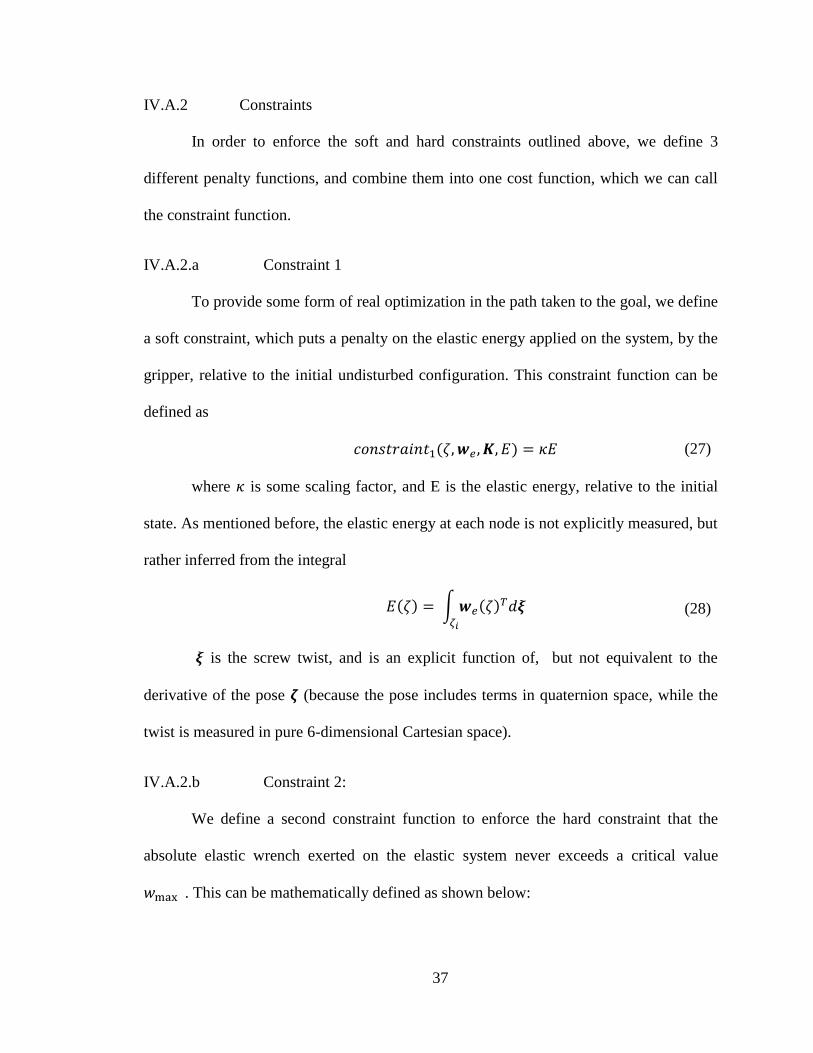
IV.A.2.a Constraint 1
To provide some form of real optimization in the path taken to the goal, we define
a soft constraint, which puts a penalty on the elastic energy applied on the system, by the
gripper, relative to the initial undisturbed configuration. This constraint function can be
defined as
( ) (27)
where is some scaling factor, and E is the elastic energy, relative to the initial
state. As mentioned before, the elastic energy at each node is not explicitly measured, but
rather inferred from the integral
( ) ∫ ( )
(28)
is the screw twist, and is an explicit function of, but not equivalent to the
derivative of the pose (because the pose includes terms in quaternion space, while the
twist is measured in pure 6-dimensional Cartesian space).
IV.A.2.b Constraint 2:
We define a second constraint function to enforce the hard constraint that the
absolute elastic wrench exerted on the elastic system never exceeds a critical value
. This can be mathematically defined as shown below:

38
( | |)
(29)
Where is a 6-dimensional weighting matrix, and is a scaling factor, and is
proportional to the constraint’s radius of influence. Plainly stated, this constraint enforces
a harsh penalty (blows up to infinity) as the magnitude of the elastic wrench approaches
the critical value
IV.A.2.c Constraint 3
In order to deal with local minima and constraint violations, we can define a 3rd
and final constraint, called the ‘red flag’ constraint. The purpose of this constraint is to
avoid moving towards known problem configurations (red-flags), such as previously
explored local minima, and locations of hard constraint violations. To do this, we create a
simple repulsive field around each of these locations. This constraint function can be
mathematically expressed as
∑
√
(30)
Where is the relative position of the red flag to the pose, and is another
scaling factor, which is proportional to the radius of influence of the constraint.
The total constraint function is just the sum of the individual constraint functions
(eq. 20).
(31)
The combined constraint function captures the penalty-avoiding behavior of each
of the individual functions.
39
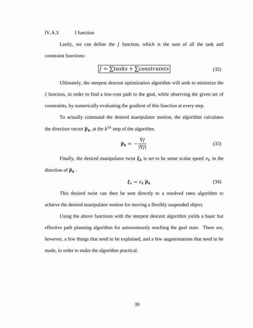
IV.A.3 J function
Lastly, we can define the function, which is the sum of all the task and
constraint functions:
(32)
Ultimately, the steepest descent optimization algorithm will seek to minimize the
J function, in order to find a low-cost path to the goal, while observing the given set of
constraints, by numerically evaluating the gradient of this function at every step.
To actually command the desired manipulator motion, the algorithm calculates
the direction vector , at the step of the algorithm.
| | (33)
Finally, the desired manipulator twist is set to be some scalar speed in the
direction of .
(34)
This desired twist can then be sent directly to a resolved rates algorithm to
achieve the desired manipulator motion for moving a flexibly suspended object.
Using the above functions with the steepest descent algorithm yields a basic but
effective path planning algorithm for autonomously reaching the goal state. There are,
however, a few things that need to be explained, and a few augmentations that need to be
made, in order to make the algorithm practical.

40
IV.B Algorithm Augmentations
IV.B.1 Dynamic Updating
At every step, the quantities of and need to be re-evaluated. The former is a
gradient of functions of the four states, and the latter is the hessian of the elastic energy
(gradient of the elastic wrench). In a very basic implementation of this algorithm, these
derivative quantities could be explicitly evaluated via their respective derivative
definitions: by perturbing the manipulator along each dimensions, and measuring the
changes in and .This implementation is time intensive, as it requires 7 additional
manipulator movements every time the quantities need to be updated.
It is possible, however, to update both of these quantities at each step, without
explicitly evaluating the derivative. The Broyden-Fletcher-Goldfarb-Shanno (BFGS) [29]
method comes from numerical optimization, and provides a way of estimating and
updating the hessian of a function, using only rank-1 gradient information. The formula
for BFGS is shown below
(
)
Where is the hessian function of ( ), is the change/gradient of the
function , and is the change in the domain of the function, . For our application,
we can set the function to the elastic energy of the system ( ). The gradient then
becomes the measured wrench , and s becomes the infinitesimal twist from the
previous step to the current step .
41
This formula will make rank-1 updates of the stiffness matrix, by evaluating the
change in wrench only along the path of travel. While this necessarily loses information
over-time about directions not along the trajectory, this lost information is arguably not as
important. Additionally, there are measures available, including minor randomization to
the trajectory, to recover lost information about the stiffness in full 6-dimensional space.
Secondly, given K which is updated at every step with BFGS, it should be noted
that the other 3 states can be integrated from position. That is,
, , ( ) (35)
Since J is explicitly only a function of ( ), it’s derivative can be
evaluated without actually perturbing the system.
( ) ( ) ( )
(36)
Using these methods, it is possible to update and estimate and K at each point
on the trajectory, without making any deviations/perturbations.
IV.B.2 Path discretization
To facilitate storage of data into memory (storing path histories at 1kHz is
impractical), as well as in updating derivatives , , the path/ path history of the
manipulator is discretized from a continuous curve to a set of nodes. This is done by
determining the next node by calculating along , and then moving along
until .
IV.B.3 Backtrack algorithm
One flaw of using an optimization algorithm like this is the susceptibility to local
minima. Another problem is how to deal with constraint violations. To solve these
42
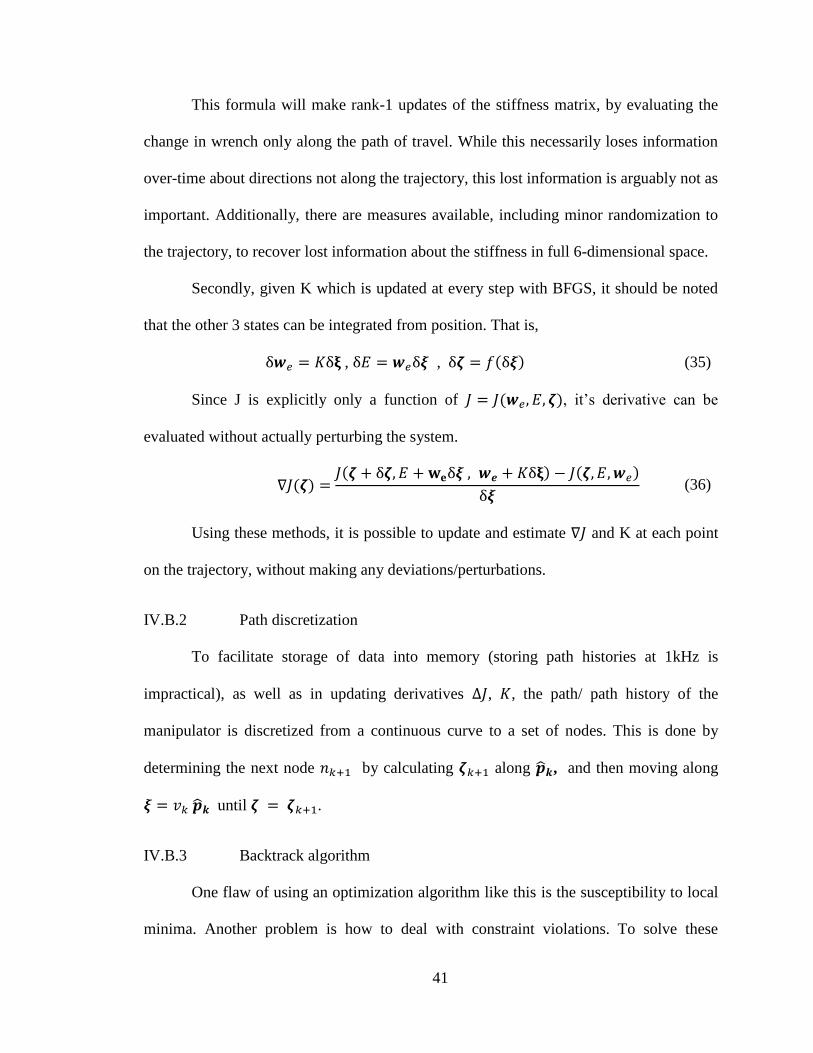
problems, a 2-part solution is implemented: Red-Flag nodes, and Backtrack/random Walk
algorithms.
As mentioned in the constraint function definition, we can label problem
configurations, nodes at which local minima are detected or where there is a constraint
violation, as a ‘red-flag’ nodes. Constraint 3 then creates repulsive fields around these
red-flag nodes, so as to avoid visiting them again.
After labeling a red-flag, a backtracking algorithm can be used return along the
recent trajectory to some previously explored node, and starting again. A random walk
algorithm can also be implemented to add a level of non-determinism to the system, to
avoid repeat configurations. To implement these solutions together, a simple Markov
Chain was defined (see section III.B.3.a), to stochastically determine when and how-
many backtracking /random walk steps should be made.
Figure 15: Backtrack Algorithm

43
The Markov Chain involves 3 states: the normal state ‘N’ ( determines next
node), ‘R’ which is a random step, and ‘B’ which moves one step back in the trajectory.
Detecting a red flag automatically sets the state as B, and initiates backtracking. The
transition probabilities were defined in order to achieve the following behavior:
In the backtracking state, probability of retaining the back-tracking state
results in the algorithm backtracking a random number of steps, with an
expected
steps, and the probability of backtracking steps being . For
60%, this results in 2.5 expected steps. After backtracking, the algorithm will
either enter a random walk, or the normal state.
In the random walk state, the probability of retaining the random walk state
results in the algorithm performing a random number of random steps, with an
expected
steps. Like the backtracking algorithm 60% results in an expected
random walk of 2.5 steps. Once the random walk is completed, the algorithm
will decay back into the Normal state.
In the Normal state, the manipulator will follow its normal trajectory, and
continue to do so with probability at each node. With a 10% probability of
retaining the normal state, the algorithm will move an expected 10 steps
normally, before making a random walk.

44
IV.C Safe Manipulation Algorithm
With the functions and augmentations defined, we can finally present the safe-
manipulation algorithm, shown in graphical form below (figure 16). At each regular step,
the algorithm evaluates the gradient , and calculates the position of the next node to
visit, and a twist-velocity to that node. Once the next node is reached, the algorithm is
iterated, and the states are updated. Unless the MDP chooses a random walk, the
algorithm will repeat itself and re-evaluate the gradient . It will repeat this procedure
until it reaches the goal state (the distance to the goal falls below ).
Figure 16: Safe Manipulation Algorithm
45
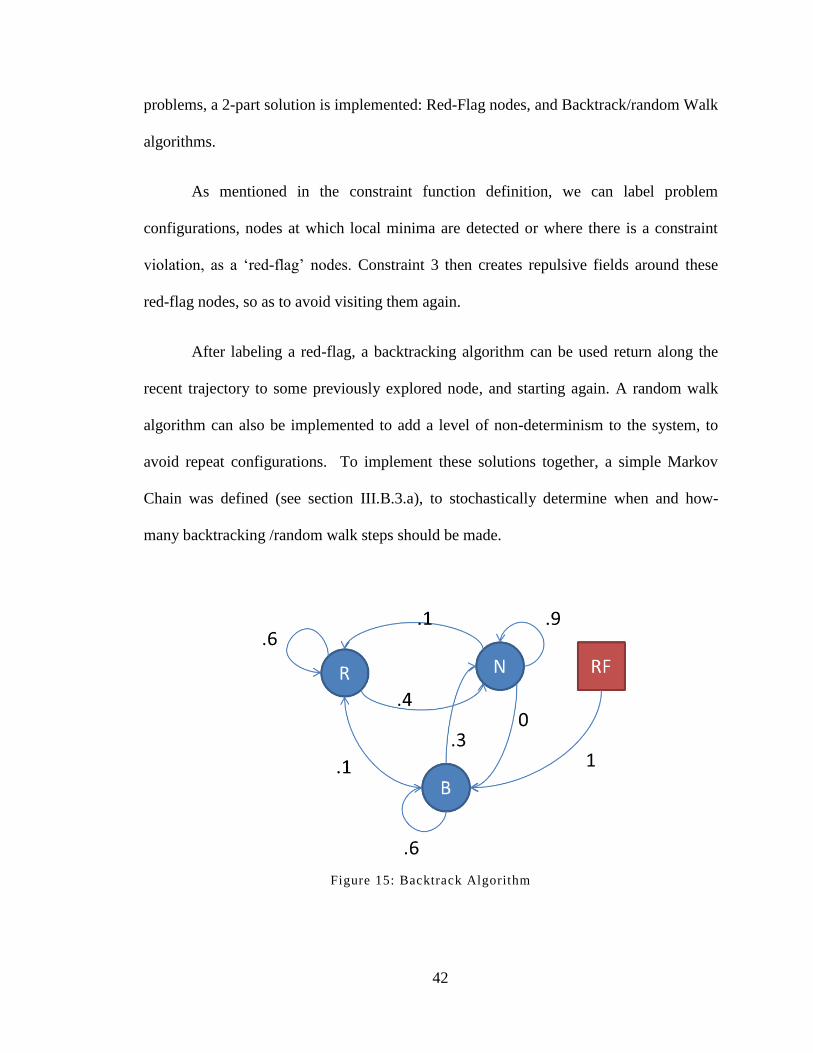
IV.D Simulation
Before experimentally testing the algorithm, it was implemented in simulation,
using a simplified planar simulation (shown below, Figure 31). In this simulation, the
object to be manipulated was a rigid planar triangle (red), attached by simple linear
springs (green) to fixed locations the ground. A manipulator (not drawn graphically), is
assumed to have perfect kinematic control over the red triangle , as well as
perfect force sensing capability , and is commanded to move the red triangle
from its initial configuration to some desired planar configuration (shown in blue).
Figure 31: Planar Robot Simulation
In order to test the ability of the algorithm to converge on the desired
configuration, two scenarios were presented. The first scenario involved setting the
desired configuration of the rigid body to a configuration which would not violate any
constraints. The other scenario was obviously to set the desired configuration to one that

46
clearly would violate the constraints if it was achieved. Below is the graphical output of
the outcome of the first scenario.
Figure 32: Planar Robot Simulation , Feasible goal
Here, the blue dots represent nodes that have been stored along the trajectory of
the rigid body, and the blue triangle represents the desired configuration of the rigid
body. Without any constraints near violation, the rigid body heads directly towards the
desired configuration and converges without issue.
0 20 40 60 80 100 1200
10
20
30
40
50
60
70
80
90
100
mm
mm
47
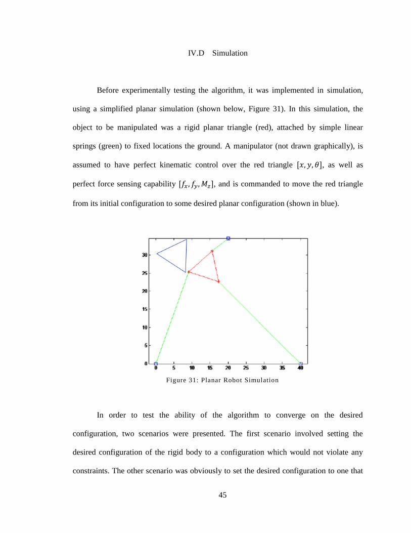
Figure 33: Error Profile, Feasible Goal
The error profile (distance to the goal) from this simulation is shown above in Figure
33.
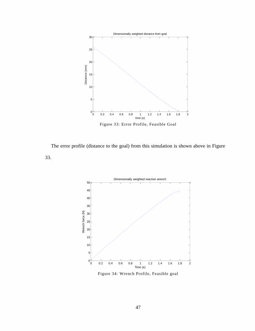
Figure 34: Wrench Profile, Feasible goal
0 0.2 0.4 0.6 0.8 1 1.2 1.4 1.6 1.8 20
5
10
15
20
25
30Dimensionally weighted distance from goal
time (s)
Dis
tam
ce (
mm
)
0 0.2 0.4 0.6 0.8 1 1.2 1.4 1.6 1.8 20
5
10
15
20
25
30
35
40
45
50Dimensionally weighted reaction wrench
Wre
nch f
orc
e (
N)
Time (s)
48
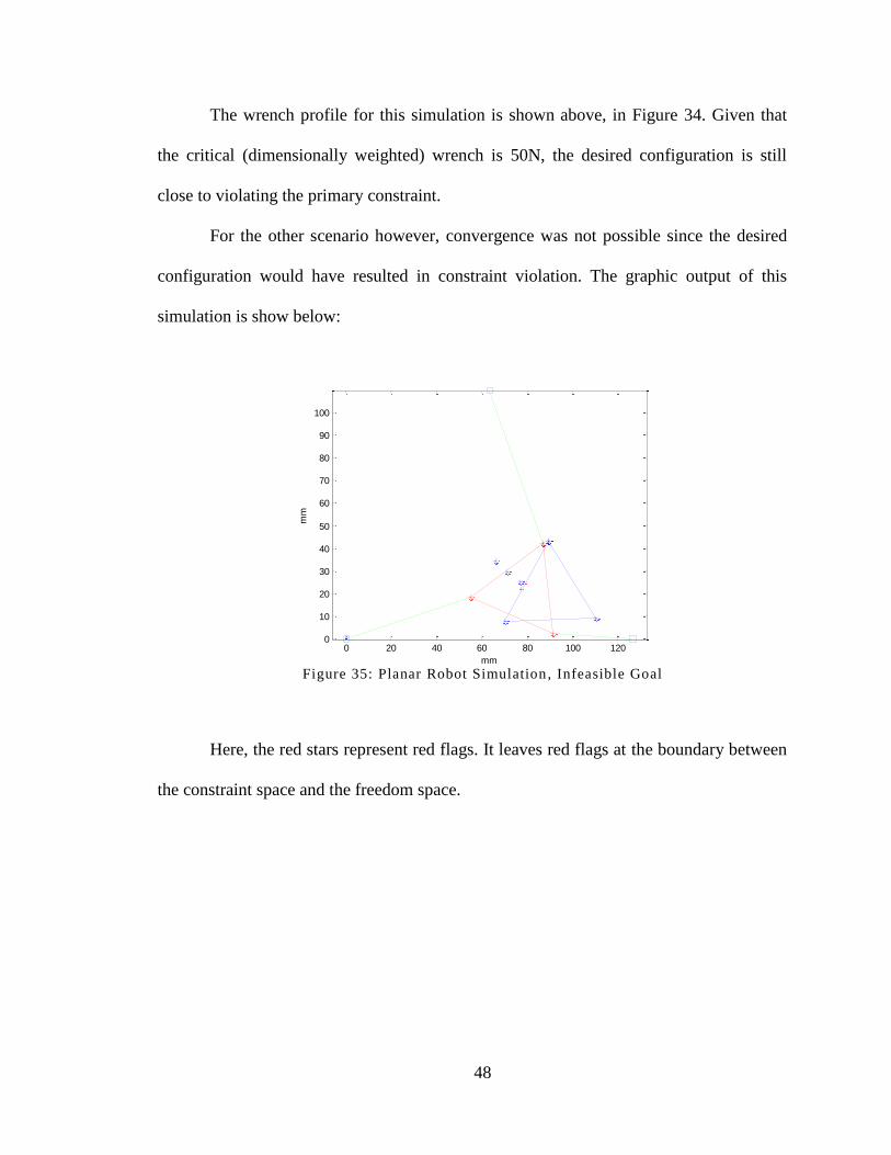
The wrench profile for this simulation is shown above, in Figure 34. Given that
the critical (dimensionally weighted) wrench is 50N, the desired configuration is still
close to violating the primary constraint.
For the other scenario however, convergence was not possible since the desired
configuration would have resulted in constraint violation. The graphic output of this
simulation is show below:
Figure 35: Planar Robot Simulation , Infeasible Goal
Here, the red stars represent red flags. It leaves red flags at the boundary between
the constraint space and the freedom space.
0 20 40 60 80 100 1200
10
20
30
40
50
60
70
80
90
100
mm
mm

49
Figure 36: Error Profile, Goal
As shown in the distance profile in Figure 36, above, the rigid body attempts to
get as close as it can to the goal, without violating the constraint. Eventually, the path
planner sends it do a configuration which does violate the constraint at around 3.25
seconds, and the rigid body is returned to the nearest safe-point.
Figure 37: Wrench Profile, Infeasible Goal
0 0.5 1 1.5 2 2.5 3 3.5 4 4.5 510
15
20
25
30
35Dimensionally weighted distance from goal
time (s)
Dis
tam
ce (
mm
)
0 0.5 1 1.5 2 2.5 3 3.5 4 4.5 50
5
10
15
20
25
30
35
40
45
50Dimensionally weighted reaction wrench
Wre
nch f
orc
e (
N)
Time (s)

50
The situation is clear when looking at the force profile in figure 37. Since the rigid
body can’t reach the desired configuration without violating the constraint, it hovers
around a configuration which lies just below the threshold for constraint violation.
IV.E Experimental Evaluation
To test this algorithm experimentally, a simple experimental mock-up of an
object, suspended in a flexible environment, was laser cut and assembled with springs, as
shown in Figure 17 below. To manipulate this object, a Puma560 industrial robot was
used, with a Gamma ATI 6-axis force sensor and a custom-made solenoid powered
gripper, designed by the author for the purposes of these experiments and manufactured
with a rapid prototyper.
Figure 17: Rigid Triangle
51
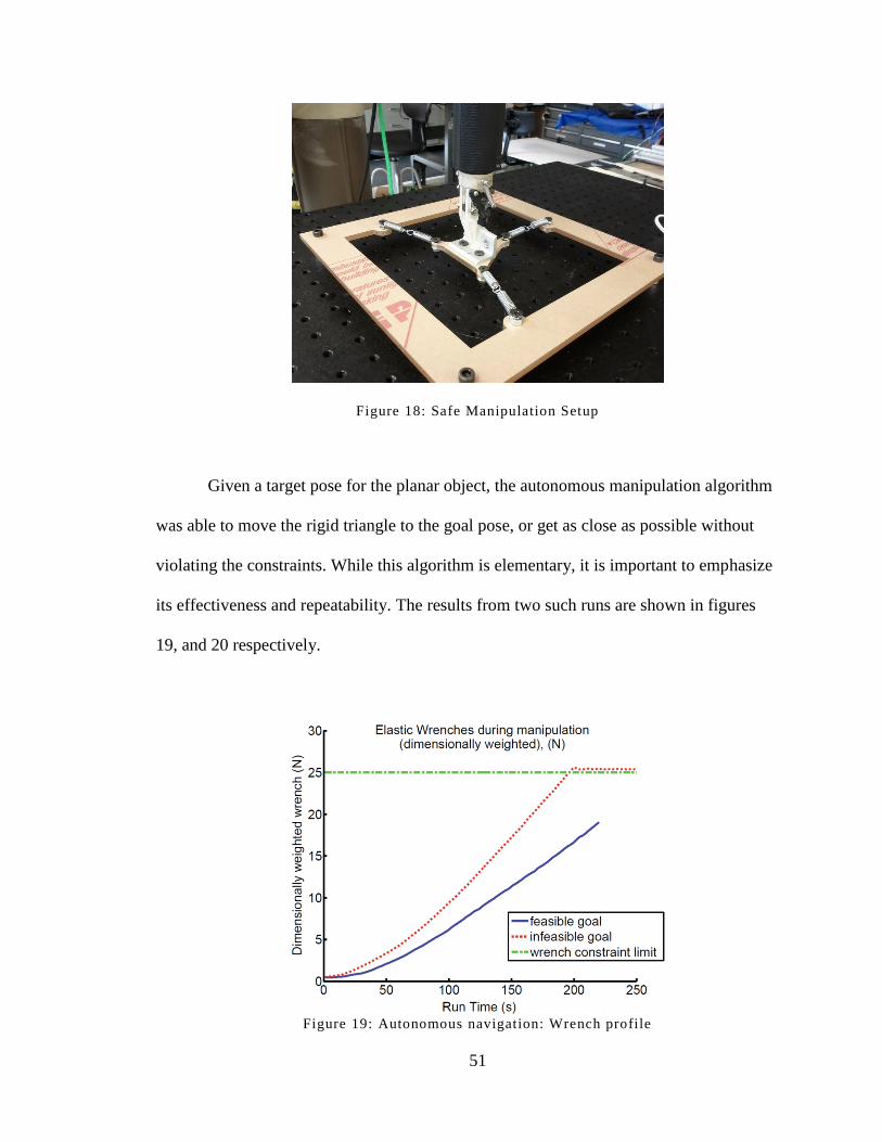
Figure 18: Safe Manipulation Setup
Given a target pose for the planar object, the autonomous manipulation algorithm
was able to move the rigid triangle to the goal pose, or get as close as possible without
violating the constraints. While this algorithm is elementary, it is important to emphasize
its effectiveness and repeatability. The results from two such runs are shown in figures
19, and 20 respectively.
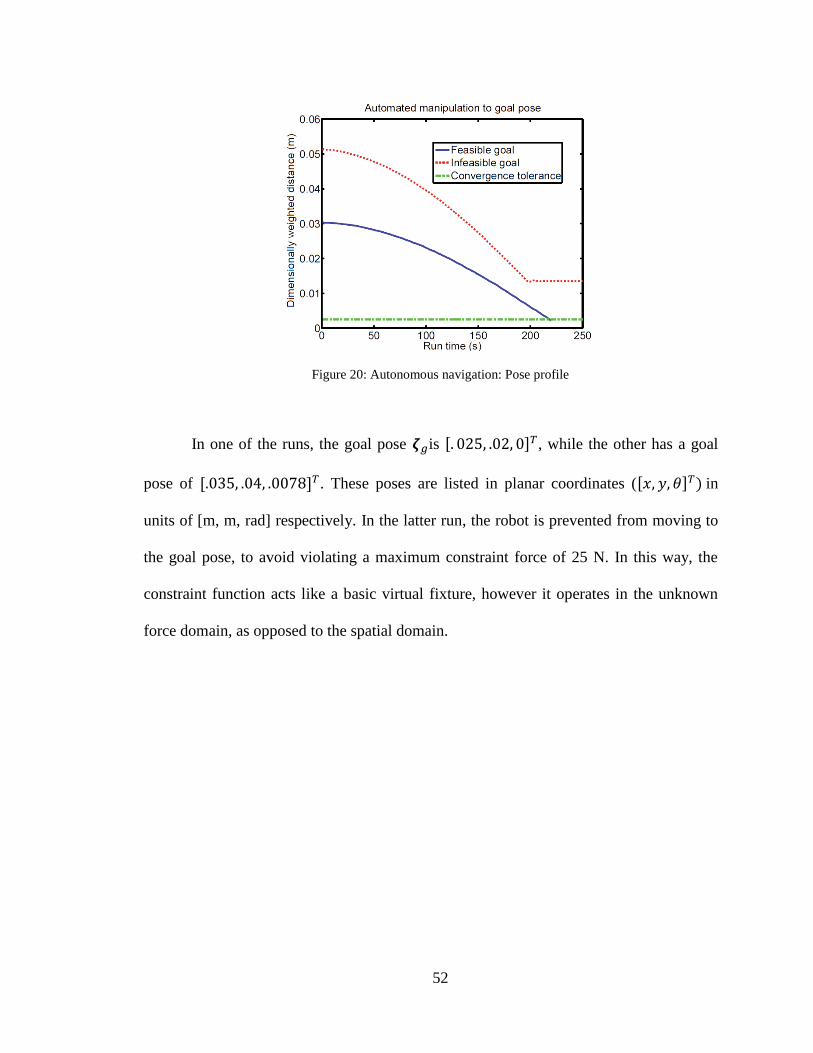
Figure 19: Autonomous navigation: Wrench profile
52
Figure 20: Autonomous navigation: Pose profile
In one of the runs, the goal pose is , while the other has a goal
pose of . These poses are listed in planar coordinates ( ) in
units of [m, m, rad] respectively. In the latter run, the robot is prevented from moving to
the goal pose, to avoid violating a maximum constraint force of 25 N. In this way, the
constraint function acts like a basic virtual fixture, however it operates in the unknown
force domain, as opposed to the spatial domain.

53
CHAPTER V
V CONSTRAINT DETECTION, CLASSIFICATION AND MAPPING
Finite element methods are currently the most popular method of representing
global stiffness properties of elastic body/environment, and they do have their
advantages. They allow complete and accurate description of the full workspace given
the necessary parameters of the system. For the application of robotic surgery however,
they are impractical. They require a-priori knowledge of the structure and parameters of
the system, and as well as localization/registration to match the numerical model with
real observed data during an operation. Most importantly however, they cannot be
implemented in real time due to significant computational costs.
Ideally, there would be some method that makes no assumptions about the
environment, (a blind algorithm), and perfectly describes the elastic behavior of the
unknown system. In practice however, to describe the elastic behavior of the system,
some information/properties have to either be assumed about the environment (not blind),
or gathered and deduced from the environment during exploration. This work takes the
latter approach, and presents an algorithm which makes no minimal about the nature of
the environment, and uses only local stiffness information during exploration of the
environment, and deduces/infers the global stiffness properties using a constraint based
model. This allows compact representation of global elastic properties, using methods
and calculations easily realizable in real time.

54
V.A Spatial Stiffness
Commonly, exploration algorithms (see Section II.B) use kinematic constraints to
determine allowable directions of motion of a manipulator in an environment, and
consider primarily rigid constraints of the form shown in Section III.A.2.
In this work, we consider the idea of flexible constraints, in which the rigid
assumption is dropped, and the kinematic constraints are no longer applicable. Unlike a
rigid constraint, a flexible constraint does not prevent motion in a given direction
(kinematic constraint), it can only impede motion in that direction. An example would be
a flexible wall versus a rigid wall. A rigid wall could be modeled as being infinitely stiff,
and thus would have the analogous kinematic constraint that a hand cannot physically
move into the wall/occupy space within the wall. For a flexible wall, the rigid
assumption is dropped, and the kinematic constraint is no longer applicable. A hand
touching a flexible wall could push into the flexible wall, given sufficient force to over-
come the impedance of the wall.
V.B Stiffness region
We seek to develop a method for characterizing the global stiffness behavior of a
specific elastic workspace. Even if we use local stiffness properties to deduce the
mechanical constraints at a given location, there can easily be multiple mechanical
constraints that operate at different locations throughout the workspace. To resolve this,
we introduce a new concept, called a stiffness region.
55
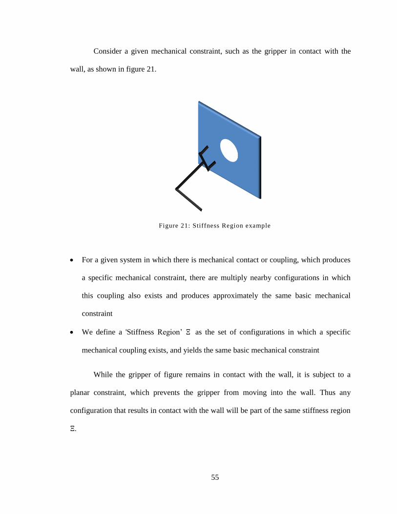
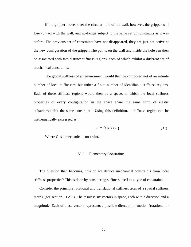
Consider a given mechanical constraint, such as the gripper in contact with the
wall, as shown in figure 21.
Figure 21: Stiffness Region example
For a given system in which there is mechanical contact or coupling, which produces
a specific mechanical constraint, there are multiply nearby configurations in which
this coupling also exists and produces approximately the same basic mechanical
constraint
We define a 'Stiffness Region’ as the set of configurations in which a specific
mechanical coupling exists, and yields the same basic mechanical constraint
While the gripper of figure remains in contact with the wall, it is subject to a
planar constraint, which prevents the gripper from moving into the wall. Thus any
configuration that results in contact with the wall will be part of the same stiffness region
.
56
If the gripper moves over the circular hole of the wall, however, the gripper will
lose contact with the wall, and no-longer subject to the same set of constraints as it was
before. The previous set of constraints have not disappeared, they are just not active at
the new configuration of the gripper. The points on the wall and inside the hole can then
be associated with two distinct stiffness regions, each of which exhibit a different set of
mechanical constraints.
The global stiffness of an environment would then be composed not of an infinite
number of local stiffnesses, but rather a finite number of identifiable stiffness regions.
Each of these stiffness regions would then be a space, in which the local stiffness
properties of every configuration in the space share the same form of elastic
behavior/exhibit the same constraint. Using this definition, a stiffness region can be
mathematically expressed as
{ | } (37)
Where C is a mechanical constraint.
V.C Elementary Constraints
The question then becomes, how do we deduce mechanical constraints from local
stiffness properties? This is done by considering stiffness itself as a type of constraint.
Consider the principle rotational and translational stiffness axes of a spatial stiffness
matrix (see section III.A.3). The result is six vectors in space, each with a direction and a
magnitude. Each of these vectors represents a possible direction of motion (rotational or

57
translational), and its associated eigenvalue represents the magnitude of the
stiffness/impedance to motion along that direction.
Accordingly, these principle axes can each be thought of as 1 degree of freedom
constraints, which impede motion along a given direction. We can call these 1 DoF
constraints ‘elementary constraints’, and the superposition of these elementary constraints
is the composite which describes the local stiffness. In fact, we can represent well known
and theoretical common constraints (See section III.2.a) as the superposition of rigid
elementary constraints.
Any of these theoretical mechanical constraints are simply a set of orthogonal
elementary constraints, which are binary (rigid or free) and frame invariant (the relation
between these constraints hold in any reference frame). The principle translational and
principle rotational stiffness of provide orthogonal sets of elementary constraints,
whose magnitudes are numerically quantified and frame invariant.
Taking advantage of this equivalence, we therefore propose representing
mechanical constraints, flexible or rigid, by the eigenvalues of the principle axes
of stiffness matrix , where represents translational
stiffness, represents rotation stiffness, and where each set is ranked in descending order.
To denote this particular representation, we call the resulting vector of eigenvalues a
Constraint vector, as shown in equation 38 below.
(38)
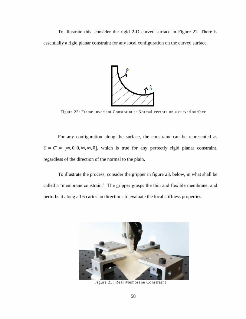
58
To illustrate this, consider the rigid 2-D curved surface in Figure 22. There is
essentially a rigid planar constraint for any local configuration on the curved surface.
Figure 22: Frame invariant Constraint s: Normal vectors on a curved surface
For any configuration along the surface, the constraint can be represented as
, which is true for any perfectly rigid planar constraint,
regardless of the direction of the normal to the plain.
To illustrate the process, consider the gripper in figure 23, below, in what shall be
called a ‘membrane constraint’. The gripper grasps the thin and flexible membrane, and
perturbs it along all 6 cartesian directions to evaluate the local stiffness properties.
Figure 23: Real Membrane Constraint
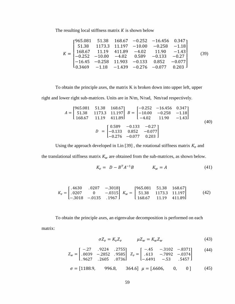
59
The resulting local stiffness matrix is shown below
[ 1 1 1 1 11 11 1 1 11 1 11
1 1 1 1 11 1
1 1 11 1 1 1
1 1 ]
(39)
To obtain the principle axes, the matrix K is broken down into upper left, upper
right and lower right sub-matrices. Units are in N/m, N/rad, Nm/rad respectively.
[ 1 1 1 1 11 11 1 1 11 1 11
] [ 1 1 1 1 11 1
]
[ 1
1
]
(40)
Using the approach developed in Lin [39] , the rotational stiffness matrix and
the translational stiffness matrix are obtained from the sub-matrices, as shown below.
(41)
[ 1 1 1 1 1
] [ 1 1 1 1 11 11 1 1 11 1 11
] (42)
To obtain the principle axes, an eigenvalue decomposition is performed on each
matrix:
(43)
[
] [ 1 1 1
1 ]
(44)
11 (45)

60
Where and are the resulting eigenvectors (principle axes) and are the
magnitudes of the principle rotational and translational stiffnesses respectively. Finally,
the constraint vector is defined as
11 (46)
As can be seen from the translational eigenvalues, there are two directions in
which motion is restricted in roughly equal magnitude, whereas there is one direction in
which motion is not impeded and negligible rotational stiffness in any direction.
Therefore, it is clear to see that the stiffness matrix does represent a membrane constraint.
V.D Constraint identification and classification
After sufficient navigation of the elastic system, as described in section IV , we
can assume set of previously visited nodes { } , each with a stiffness
matrix and an associated constraint vector . To classify these constraints vectors, we
can use the k-means algorithm (see section III.B.2) to break the set of nodes (examples)
into a set of similar classes. The number of classes will be the number of constraints in
the system, and the set of nodes in each class will be defined as a stiffness region, for that
class.
In order to adapt the k-means algorithm to this problem, several small
augmentations need to be made. Firstly, each constraint vector contains a set of
translational stiffnesses, and a set of rotational stiffnesses, each with its own set of units.
To scale/balance the units, the dimensional weighting factor can be used (see section
IV.A.1) to scale rotational stiffnesses, such that
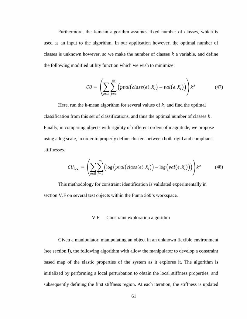
61
Furthermore, the k-mean algorithm assumes fixed number of classes, which is
used as an input to the algorithm. In our application however, the optimal number of
classes is unknown however, so we make the number of classes a variable, and define
the following modified utility function which we wish to minimize:
(∑ ∑ ( )
) (47)
Here, run the k-mean algorithm for several values of , and find the optimal
classification from this set of classifications, and thus the optimal number of classes .
Finally, in comparing objects with rigidity of different orders of magnitude, we propose
using a log scale, in order to properly define clusters between both rigid and compliant
stiffnesses.
(∑ ∑ ( )
) (48)
This methodology for constraint identification is validated experimentally in
section V.F on several test objects within the Puma 560’s workspace.
V.E Constraint exploration algorithm
Given a manipulator, manipulating an object in an unknown flexible environment
(see section I), the following algorithm with allow the manipulator to develop a constraint
based map of the elastic properties of the system as it explores it. The algorithm is
initialized by performing a local perturbation to obtain the local stiffness properties, and
subsequently defining the first stiffness region. At each iteration, the stiffness is updated
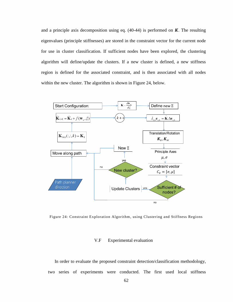
62
and a principle axis decomposition using eq. (40-44) is performed on . The resulting
eigenvalues (principle stiffnesses) are stored in the constraint vector for the current node
for use in cluster classification. If sufficient nodes have been explored, the clustering
algorithm will define/update the clusters. If a new cluster is defined, a new stiffness
region is defined for the associated constraint, and is then associated with all nodes
within the new cluster. The algorithm is shown in Figure 24, below.
Figure 24: Constraint Exploration Algorithm, using Clustering and Stiffness Regions
V.F Experimental evaluation
In order to evaluate the proposed constraint detection/classification methodology,
two series of experiments were conducted. The first used local stiffness
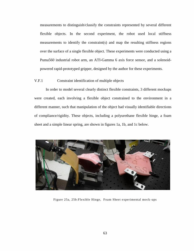
63
measurements to distinguish/classify the constraints represented by several different
flexible objects. In the second experiment, the robot used local stiffness
measurements to identify the constraint(s) and map the resulting stiffness regions
over the surface of a single flexible object. These experiments were conducted using a
Puma560 industrial robot arm, an ATI-Gamma 6 axis force sensor, and a solenoid-
powered rapid-prototyped gripper, designed by the author for these experiments.
V.F.1 Constraint identification of multiple objects
In order to model several clearly distinct flexible constraints, 3 different mockups
were created, each involving a flexible object constrained to the environment in a
different manner, such that manipulation of the object had visually identifiable directions
of compliance/rigidity. These objects, including a polyurethane flexible hinge, a foam
sheet and a simple linear spring, are shown in figures 1a, 1b, and 1c below.
Figure 25a, 25b:Flexible Hinge, Foam Sheet experimental mock -ups
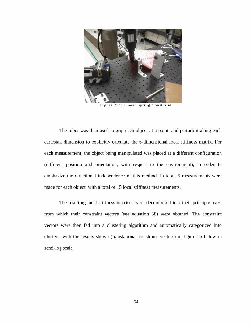
64
Figure 25c: Linear Spring Constraint
The robot was then used to grip each object at a point, and perturb it along each
cartesian dimension to explicitly calculate the 6-dimensional local stiffness matrix. For
each measurement, the object being manipulated was placed at a different configuration
(different position and orientation, with respect to the environment), in order to
emphasize the directional independence of this method. In total, 5 measurements were
made for each object, with a total of 15 local stiffness measurements.
The resulting local stiffness matrices were decomposed into their principle axes,
from which their constraint vectors (see equation 38) were obtaned. The constraint
vectors were then fed into a clustering algorithm and automatically categorized into
clusters, with the results shown (translational constraint vectors) in figure 26 below in
semi-log scale.

65
Figure 26: Constraint identification using clustering
The clustering algorithm broke the 15 measurements into 3 clusters (red, blue and
black), correctly categorizing all 5 measurements corresponding to each object into its
own cluster. The blue cluster corresponds to the linear spring, the red to the flexible
hinge, and the black to the foam sheet. It should be noted that this clustering was obtained
from the global optimal clustering (global minimum of ). This is important, as the
traditional k-means algorithm (see section III.B.2) uses a local optimizer, whereas
particle filtering (section III.B.3) was used here to find the global minimum.
The constraint vectors plotted in Figure 26 are shown below in tabular form,
along with the average of their associated clusters.
102
103
104
102
103
104
101
102
103
Min
or
Axis
Stiff
ness(N
/m)
3-dimensional feature space: 3 object constraint identification
Major Axis Stiffness (N/m)Mid Axis Stiffness (N/m)
Linear Spring Foam Sheet
Flexible Hinge
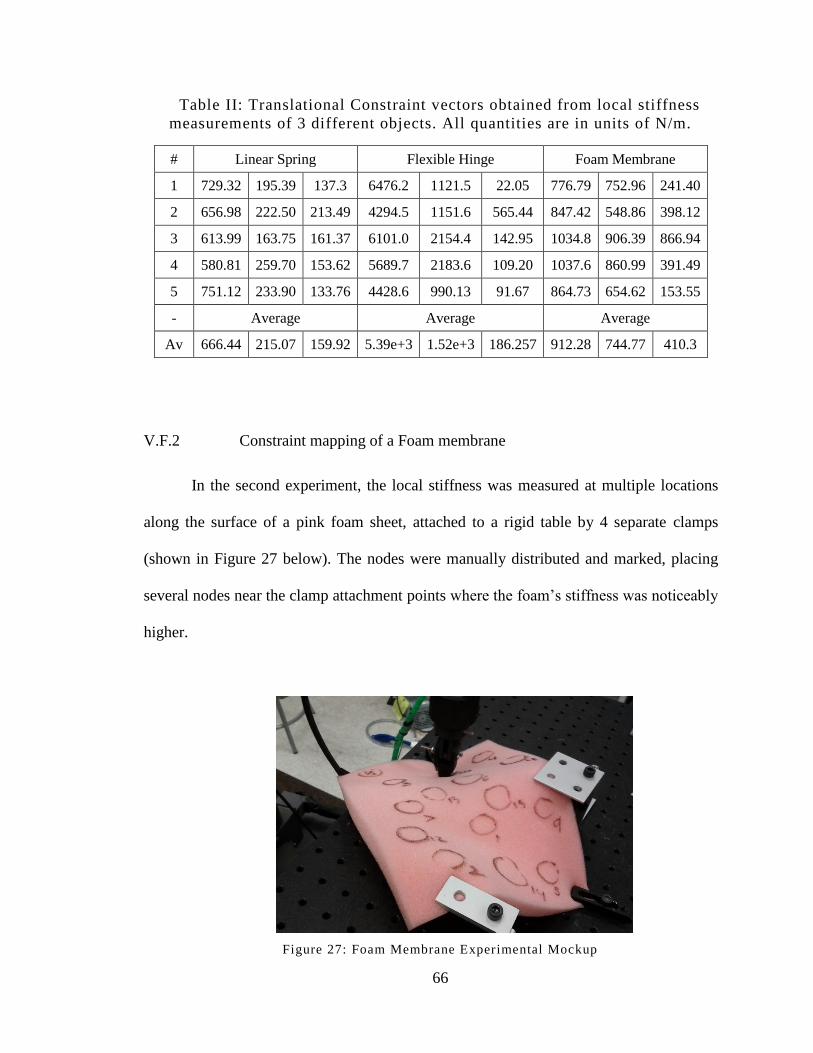
66
Table II: Translational Constraint vectors obtained from local stiffness
measurements of 3 different objects. All quantities are in units of N/m.
# Linear Spring Flexible Hinge Foam Membrane
1 729.32 195.39 137.3 6476.2 1121.5 22.05 776.79 752.96 241.40
2 656.98 222.50 213.49 4294.5 1151.6 565.44 847.42 548.86 398.12
3 613.99 163.75 161.37 6101.0 2154.4 142.95 1034.8 906.39 866.94
4 580.81 259.70 153.62 5689.7 2183.6 109.20 1037.6 860.99 391.49
5 751.12 233.90 133.76 4428.6 990.13 91.67 864.73 654.62 153.55
- Average Average Average
Av 666.44 215.07 159.92 5.39e+3 1.52e+3 186.257 912.28 744.77 410.3
V.F.2 Constraint mapping of a Foam membrane
In the second experiment, the local stiffness was measured at multiple locations
along the surface of a pink foam sheet, attached to a rigid table by 4 separate clamps
(shown in Figure 27 below). The nodes were manually distributed and marked, placing
several nodes near the clamp attachment points where the foam’s stiffness was noticeably
higher.
Figure 27: Foam Membrane Experimental Mockup

67
As with the previous experiment, the resulting local stiffness matrices were
decomposed into their principle axes, and the associated constraint vectors were then fed
into the same clustering algorithm, which automatically cateogorized the data into a set of
clusters, as shown below (Figure 28).
Figure 28: Constraint detection using clustering, Foam sheet
Using linear scale clustering algorithm [30] (as opposed to log scale), the
algorithm identified 2 primary clusters, shown in blue and red. The blue cluster
corresponds roughly to a membrane constraint, in which translation is impeded in a
plane, whereas movement along the normal is fairly complaint. The cluster in red,
however, corresponds to a more homogeneous stiffness, in which no axis in particular is
negligible. There were two particular nodes in the middle, which were either one of the
600800
10001200
14001600
1800 400600
8001000
1200100
200
300
400
500
600
700
800
900
Min
or
axis
stiff
ness (
N/m
)
3 dimensional feature space: Foam bed
Major axis stiffness (N/m)
Mid axis stiffness (N/m)
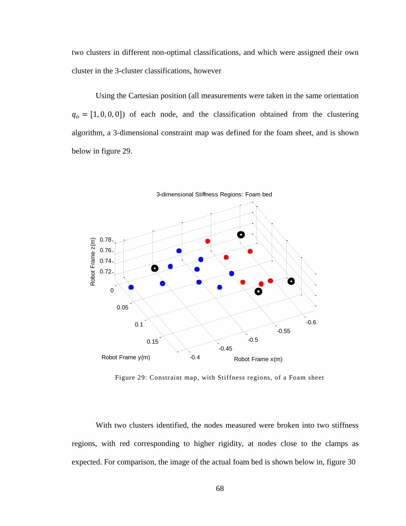
68
two clusters in different non-optimal classifications, and which were assigned their own
cluster in the 3-cluster classifications, however
Using the Cartesian position (all measurements were taken in the same orientation
1 ) of each node, and the classification obtained from the clustering
algorithm, a 3-dimensional constraint map was defined for the foam sheet, and is shown
below in figure 29.
Figure 29: Constraint map, with Stiffness regions, of a Foam sheet
With two clusters identified, the nodes measured were broken into two stiffness
regions, with red corresponding to higher rigidity, at nodes close to the clamps as
expected. For comparison, the image of the actual foam bed is shown below in, figure 30
-0.6
-0.55
-0.5
-0.45
-0.4
0
0.05
0.1
0.15
0.72
0.74
0.76
0.78
Robot
Fra
me z
(m)
3-dimensional Stiffness Regions: Foam bed
Robot Frame x(m)Robot Frame y(m)
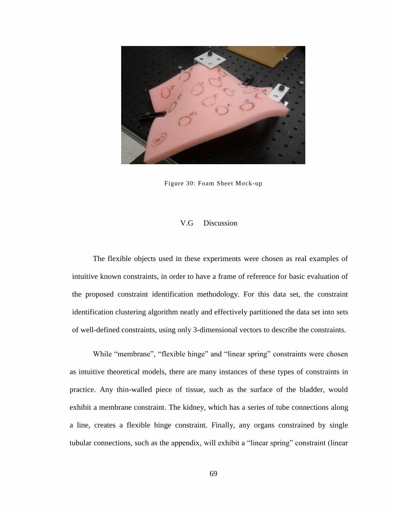
69
Figure 30: Foam Sheet Mock-up
V.G Discussion
The flexible objects used in these experiments were chosen as real examples of
intuitive known constraints, in order to have a frame of reference for basic evaluation of
the proposed constraint identification methodology. For this data set, the constraint
identification clustering algorithm neatly and effectively partitioned the data set into sets
of well-defined constraints, using only 3-dimensional vectors to describe the constraints.
While “membrane”, “flexible hinge” and “linear spring” constraints were chosen
as intuitive theoretical models, there are many instances of these types of constraints in
practice. Any thin-walled piece of tissue, such as the surface of the bladder, would
exhibit a membrane constraint. The kidney, which has a series of tube connections along
a line, creates a flexible hinge constraint. Finally, any organs constrained by single
tubular connections, such as the appendix, will exhibit a “linear spring” constraint (linear
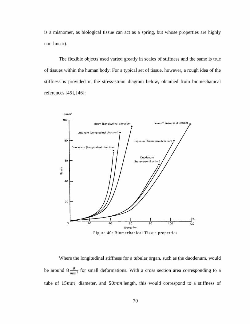
70
is a misnomer, as biological tissue can act as a spring, but whose properties are highly
non-linear).
The flexible objects used varied greatly in scales of stiffness and the same is true
of tissues within the human body. For a typical set of tissue, however, a rough idea of the
stiffness is provided in the stress-strain diagram below, obtained from biomechanical
references [45], [46]:
Figure 40: Biomechanical Tissue properties
Where the longitudinal stiffness for a tubular organ, such as the duodenum, would
be around
for small deformations. With a cross section area corresponding to a
tube of 1 diameter, and length, this would correspond to a stiffness of

71
, which resides on the low side of the stiffness measurements founds in these
experiments, however it is on the same/similar order of magnitude. Therefore, from the
preliminary results, it would be safe to conclude that the presented constraint vector
classification methodology is capable of identifying/differentiating between basic flexible
constraints, using only local stiffness measurements. More thorough
evaluation/performance analysis of these methods is left as future work.
72
CHAPTER VI
VI CONCLUSION
In this thesis, Algorithms for blind, safe, autonomous manipulation in unknown
flexible environments were presented. A solution was proposed, using state-based
cost/reward functions and force/based constraints/virtual fixtures, and was subsequently
verified using a custom-fabricated planar mock-up of an elastic environment. Secondly,
compact representation of global stiffness was presented via the use of stiffness regions
and constraint maps, and real-time constraint detection/identification/classification was
achieved using constraint vectors, 6-dimensional frame-invariant vectors derived from
local stiffness measurements. These methods were evaluated using local stiffness
measurements of several different flexible objects, each with its own constraint(s). A
clustering algorithm was able to correctly classify/group together the stiffness
measurements from 3 different flexible objects, and was furthermore able to define a
constraint map, highlighting two distinct stiffness regions, over the surface of a
particular flexible object.
Given the reasonable set of objects used in the constraint identification
experiments, it would be safe to say that constraint vector clustering is at least capable of
discerning/classifying constraints of basic flexible objects. The primary weakness of
such a technique would be the situation of varied but smoothly changing stiffness
properties, in which the constraint vectors would form a large continuous data set, and
would result in poor cluster classifications. In such a situation, Principle component
73
Analysis might provide a much better framework for organizing/classifying the
constraints. Using a log scale clustering however, the cluster technique is perfectly
capable of discerning/identifying hard rigid constraints (bone) free space (air) and
anything in between.
The utility of the approaches presented in this Thesis would truly be realized by
integrating the constraint identification/mapping with the safe-manipulation algorithm.
The target approach would be to use explored stiffness regions to make non-local
trajectory optimization, by predicting the force, stiffness and elasticity many steps ahead
of the local configuration.
While the approaches presented are blind, they could be enhanced with a-priori
information. If the clustering classification algorithm is given a set of training data
(previously obtained experimental data from similar environments), it could be used for
haptic exploration and localization. The target application would be in searching for a
constraint, which is known to exist in the workspace, but whose location in the
workspace is unknown (such as searching for a tumor/cyst on an organ).
Blind, safe manipulation in flexible environments, used in tandem with real time
constraint identification/mapping, will allow a robot to simultaneously explore,
characterize, and manipulate an elastic system safely without a-priori knowledge. This
approach, if developed further, could eventually enable safe semi-autonomous
cooperative manipulation of RSAs in applications such as organ retraction and organ
manipulation, during surgical procedures.
74
BIBLIOGRAPHY
1. Guthart, Gary S, and J Kenneth Salisbury. “The Intuitive TM Telesurgery
System : Overview and Application.” In IEEE International Conference on
Robotics and Automation, 2-5, 2000.
2. Ding, Jienan, Kai Xu, Roger Goldman, Peter Allen, Dennis Fowler, and Nabil
Simaan. “Design , Simulation and Evaluation of Kinematic Alternatives for
Insertable Robotic Effectors Platforms in Single Port Access Surgery.” In
IEEE International Conference on Robotics and Automation, 2-7, 2010.
3. Abbott, D.J., Chris Becke, R.I. Rothstein, and W.J. Peine. “Design of an
endoluminal NOTES robotic system.” In Intelligent Robots and Systems, 2007.
IROS 2007. IEEE/RSJ International Conference on, 410–416. IEEE, 2007.
http://ieeexplore.ieee.org/xpls/abs_all.jsp?arnumber=4399536.
4. Degani, Amir, Howie Choset, Brett Zubiate, Takeyoshi Ota, and Marco Zenati.
“Highly articulated robotic probe for minimally invasive surgery.” In IEEE
International Conference on Robotics and Automation, 3273-6, 2006.
http://www.ncbi.nlm.nih.gov/pubmed/19163406.
5. Xiao, Jing. “Automatic Determination of Topological Contacts in the Presence
of Sensing Uncertainties *.” In IEEE International Conference on Robotics
and Automation, 65-70, 1993.
6. Xiao, J. “Automatic Generation of High-Level Contact State Space.” The
International Journal of Robotics Research 20, no. 7 (July 1, 2001): 584-606.
http://ijr.sagepub.com/cgi/doi/10.1177/02783640122067552.
7. Bruyninckx, Herman, and Joris De Schutter. “Kinematic Models of Rigid
Body Interactions for Uncertainties.” In IEEE International Conference on
Robotics and Automation, 1007-1012, 1993.
8. Kitagaki, K., T. Ogasawara, and T. Suehiro. “Contact state detection by force
sensing for assembly tasks.” In IEEE International Conference on Multisensor
Fusion and Integration for Intelligent Systems, 366-370. Ieee, 1994.
http://ieeexplore.ieee.org/lpdocs/epic03/wrapper.htm?arnumber=398431.
9. Dupont, Pierre E, Timothy M Schulteis, and D Howe. “Experimental
Identification of Kinematic Constraints.” In IEEE International Conference on
Robotics and Automation, 2677-2682, 1997.
10. Debus, Thomas J., Pierre E. Dupont, and Robert D. Howe. “Contact State
Estimation Using Multiple Model Estimation and Hidden Markov Models.”
The International Journal of Robotics Research 23, no. 4 (April 1, 2004): 399-
413. http://ijr.sagepub.com/cgi/doi/10.1177/0278364904042195.
75
11. Okamura, a. M. “Feature Detection for Haptic Exploration with Robotic
Fingers.” The International Journal of Robotics Research 20, no. 12
(December 1, 2001): 925-938.
http://ijr.sagepub.com/cgi/doi/10.1177/02783640122068191.
12. Okamura, A M, M L Turner, and M R Cutkoslcy. “- Haptic Exploration of
Objects with Rolling and Sliding.” In IEEE International Conference on
Robotics and Automation, 2485-2490, 1997.
13. Allen, P.K., and K.S. Roberts. “Haptic object recognition using a multi-
fingered dextrous hand.” In Proceedings, 1989 International Conference on
Robotics and Automation, 342-347. IEEE Comput. Soc. Press, 1989.
http://ieeexplore.ieee.org/lpdocs/epic03/wrapper.htm?arnumber=100011.
14. Liu, Hongbin, Jichun Li, Xiaojing Song, Lakmal D Seneviratne, and Kaspar
Althoefer. “Identification During Minimally Invasive Surgery.” In IEEE
transactions on robotics, 27:450-460, 2011.
15. Xu, Kai, Student Member, and Nabil Simaan. “An Investigation of the Intrinsic
Force Sensing Capabilities of Continuum Robots.” In IEEE International
Conference on Robotics and Automation, 24:576-587, 2008.
16. Mehrandezh, M., and K.K. Gupta. “Simultaneous path planning and free space
exploration with skin sensor.” In Proceedings 2002 IEEE International
Conference on Robotics and Automation (Cat. No.02CH37292), 4:3838-3843.
Ieee, 2002.
http://ieeexplore.ieee.org/lpdocs/epic03/wrapper.htm?arnumber=1014319.
17. Rodriguez, S., J.M. Lien, and N.M. Amato. “Planning motion in completely
deformable environments.” In Robotics and Automation, 2006. ICRA 2006.
Proceedings 2006 IEEE International Conference on, 2466–2471. IEEE, 2006.
http://ieeexplore.ieee.org/xpls/abs_all.jsp?arnumber=1642072.
18. Patil, Sachin, and Ron Alterovitz. “Toward automated tissue retraction in
robot-assisted surgery.” In Robotics and Automation (ICRA), 2010 IEEE
International Conference on, 2088–2094. IEEE, 2010.
http://ieeexplore.ieee.org/xpls/abs_all.jsp?arnumber=5509607.
19. Gayle, Russell, Paul Segars, MC Lin, and D. Manocha. “Path planning for
deformable robots in complex environments.” In Proc. of Robotics: Science
and Systems (RSS), 225–232. Citeseer, 2005.
http://citeseerx.ist.psu.edu/viewdoc/download?doi=10.1.1.104.1601&rep=
rep1&type=pdf.
20. Huang, Shuguang, and J.M. Schimmels. “The bounds and realization of spatial
stiffnesses achieved with simple springs connected in parallel.” In Robotics
and Automation, IEEE Transactions on, 14:466–475. IEEE, 1998.
http://ieeexplore.ieee.org/xpls/abs_all.jsp?arnumber=678455.
76
21. Roberts, R.G. “Minimal realization of a spatial stiffness matrix with simple
springs connected in parallel.” In Robotics and Automation, IEEE Transactions
on, 15:953–958. IEEE, 1999.
http://ieeexplore.ieee.org/xpls/abs_all.jsp?arnumber=795799.
22. Roberts, R.G. “Minimal realization of an arbitrary spatial stiffness matrix with
a parallel connection of simple and complex springs.” In Robotics and
Automation, IEEE Transactions on, 16:603–608. IEEE, 2000.
http://ieeexplore.ieee.org/xpls/abs_all.jsp?arnumber=880811.
23. Ciblak, Namik, and H. Lipkin. “Synthesis of Cartesian stiffness for robotic
applications.” In Robotics and Automation, 1999. Proceedings. 1999 IEEE
International Conference on, 3:2147–2152. IEEE, 1999.
http://ieeexplore.ieee.org/xpls/abs_all.jsp?arnumber=770424.
24. Huang, Shuguang, and Joseph M Schimmels. “The Eigenscrew Decomposition
of Spatial.” In IEEE Transactions on Robotics and Automation, 6:146-156,
2000.
25. McAllister, PL. “An eigenscrew analysis of mechanism compliance.” Robotics
and Automation, 2000. (2000).
http://ieeexplore.ieee.org/xpls/abs_all.jsp?arnumber=845173.
26. Lipkin, Harvey, and Timothy Patterson. “Generalized center of compliance
and stiffness.” In IEEE International Conference on Robotics and Automation,
54:1161-1164, 1992. http://www.ncbi.nlm.nih.gov/pubmed/19962288.
27. Higham, NJ. “Computing a nearest symmetric positive semidefinite matrix.”
Linear algebra and its applications 118 (1988).
http://www.sciencedirect.com/science/article/pii/0024379588902236.
28. F. Fahimi Autonomous Robots: Modeling, Path Planning and Control, New
York, NY, Springer Science + Business Media , 2009
29. J. Nocedal and S. J. Wright, Numerical Optimization, New York NY,
Springer-Verlag (1999)
30. Poole, David L., and Alan K. Mackworth. Artificial Intelligence: Foundations
of Computational Agents. New York, NY: Cambridge University PRess, 2010.
31. Korf, Richard E. “Real-time heuristic search.” Artificial Intelligence 42, no. 2-
3 (March 1990): 189-211.
http://linkinghub.elsevier.com/retrieve/pii/0004370290900544.
32. Griffis, Michael, and J. Duffy. “Comparing structures of stiffness matrices
using invariants.” RoManSy 9, no. 3 (1993): 85–92.
http://www.springerlink.com/index/M685515657663T85.pdf.
33. Ma, Burton, and R. Ellis. “Spatial-stiffness analysis of surface-based
registration.” Medical Image Computing and Computer-Assisted Intervention–
77
MICCAI 2004, no. 1 (2004): 623–630.
http://www.springerlink.com/index/HEYHPN967Q5TJFAE.pdf.
34. Yuan, JS. “Closed-loop manipulator control using quaternion feedback.”
Robotics and Automation, IEEE Journal of 4, no. 4 (1988): 434–440.
http://ieeexplore.ieee.org/xpls/abs_all.jsp?arnumber=809.
35. A. Petrovskaya, O. Khatib, S. Thrun, and A. Y. Ng. “Bayesian estimation for
autonomous object manipulation based on tactile sensors” Proceedings of the
2006 IEEE International Conference on Robotics and Automation, 2006
36. Goldman, R. E., Bajo, A. & Simaan, N (2011). Compliant Motion Control for
Continuum Robots with Intrinsic Actuation Sensing. In 2011 IEEE
International Conference on Robotics and Automation, pages 1126-1132.
Shanghai, China.
37. Goldman, R. (2011). Analysis, Algorithms, and Control for Intelligent Surgical
Exploration and Intervention. Phd Thesis, Columbia University
38. Yamamoto, Tomonori, Balazs Vagvolgyi, Kamini Balaji, Louis L. Whitcomb,
and Allison M. Okamura. “Tissue property estimation and graphical display
for teleoperated robot-assisted surgery.” 2009 IEEE International Conference
on Robotics and Automation (May 2009): 4239-4245.
http://ieeexplore.ieee.org/lpdocs/epic03/wrapper.htm?arnumber=5152674.
39. Lin, Q., J.W. Burdick, and E. Rimon. “A stiffness-based quality measure for
compliant grasps and fixtures.” IEEE Transactions on Robotics and
Automation 16, no. 6 (2000): 675-688.
http://ieeexplore.ieee.org/lpdocs/epic03/wrapper.htm?arnumber=897779.
40. Arora, J.S., Introduction to Optimum Design, Second Edition, Elsevier
Academic Press, 2004.
41. Rosen, Jacob, Jeffrey D Brown, Lily Chang, Mika N Sinanan, and Blake
Hannaford. “Generalized approach for modeling minimally invasive surgery as
a stochastic process using a discrete Markov model.” In IEEE transactions on
bio-medical engineering, 53:399-413, 2006.
http://www.ncbi.nlm.nih.gov/pubmed/16532766.
42. Hart, John C., George K. Francis, and Louis H. Kauffman. “Visualizing
quaternion rotation.” ACM Transactions on Graphics 13, no. 3 (July 1, 1994):
256-276. http://portal.acm.org/citation.cfm?doid=195784.197480.
43. Kuipers, Jack. B. Quaternions and Rotation Sequences. 2nd ed. Princeton, NJ:
Princeton University Press, 1999.
44. Lefebvre, Tine, Herman Bruyninckx, and J. De Schutter. “Polyhedral contact
formation identification for autonomous compliant motion: Exact nonlinear
78
Bayesian filtering.” Robotics, IEEE Transactions on 21, no. 1 (2005): 124–
129.
45. Yamada, H. Strength of Biological Material, Baltimore, William&Wilkins
(1970)
46. Y.C. Fung Biomechanics: Mechanical Properties of Living Tissues, New
York, NY, Springer (1993)
47. Bajo, A., Goldman, R. E. & Simaan, N (2011). Configuration and Joint
Feedback for Enhanced Performance of Multi-Segment Continuum Robots. In
2011 IEEE International Conference on Robotics and Automation, pages
2905-2912. Shanghai,
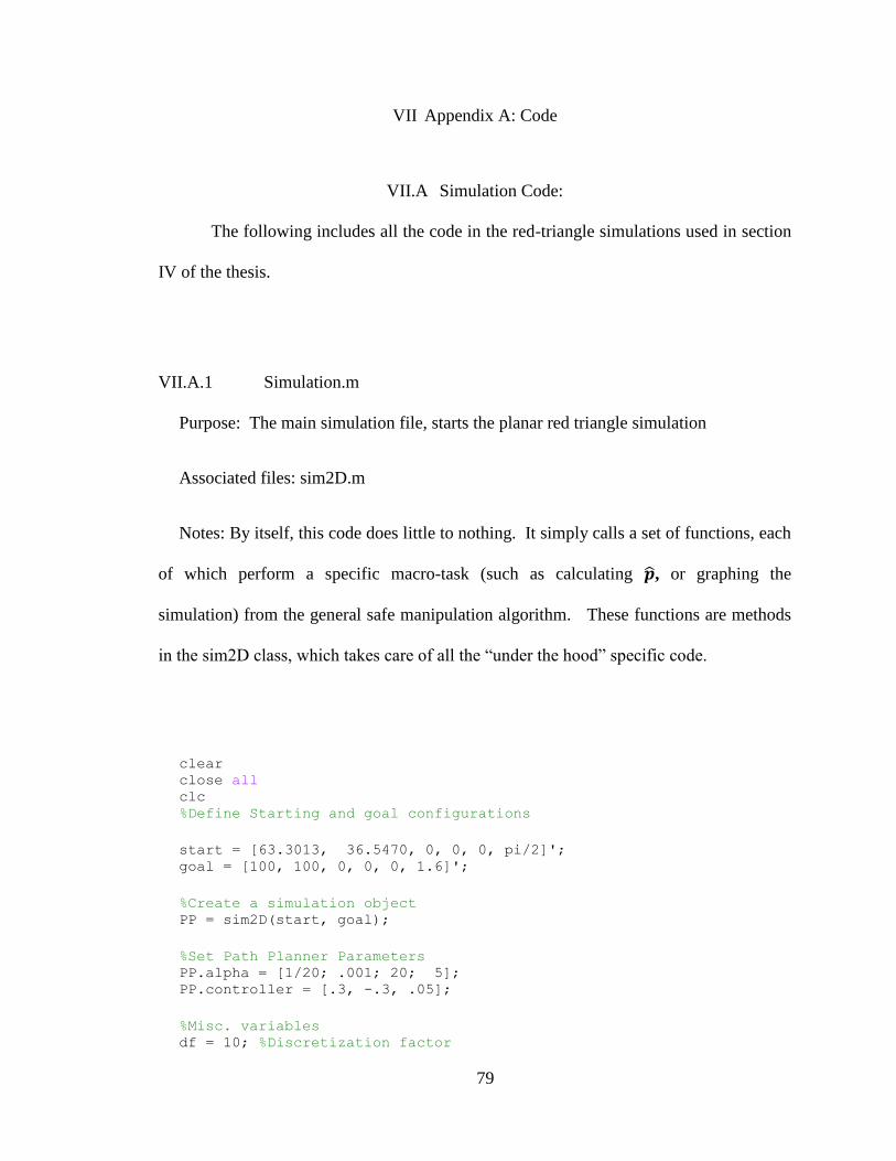
79
VII Appendix A: Code
VII.A Simulation Code:
The following includes all the code in the red-triangle simulations used in section
IV of the thesis.
VII.A.1 Simulation.m
Purpose: The main simulation file, starts the planar red triangle simulation
Associated files: sim2D.m
Notes: By itself, this code does little to nothing. It simply calls a set of functions, each
of which perform a specific macro-task (such as calculating , or graphing the
simulation) from the general safe manipulation algorithm. These functions are methods
in the sim2D class, which takes care of all the “under the hood” specific code.
clear close all clc %Define Starting and goal configurations
start = [63.3013, 36.5470, 0, 0, 0, pi/2]'; goal = [100, 100, 0, 0, 0, 1.6]';
%Create a simulation object PP = sim2D(start, goal);
%Set Path Planner Parameters PP.alpha = [1/20; .001; 20; 5]; PP.controller = [.3, -.3, .05];
%Misc. variables df = 10; %Discretization factor
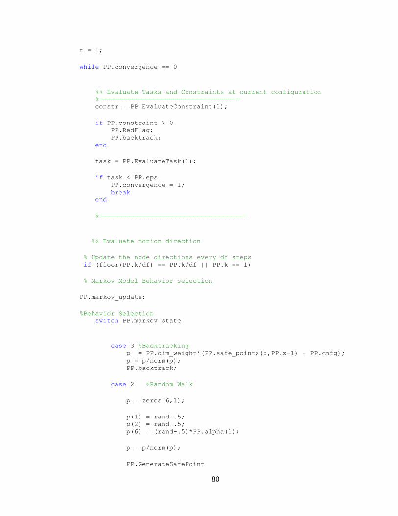
80
t = 1;
while PP.convergence == 0
%% Evaluate Tasks and Constraints at current configuration %------------------------------------ constr = PP.EvaluateConstraint(1);
if PP.constraint > 0 PP.RedFlag; PP.backtrack; end
task = PP.EvaluateTask(1);
if task < PP.eps PP.convergence = 1; break end
%--------------------------------------
%% Evaluate motion direction
% Update the node directions every df steps if (floor(PP.k/df) == PP.k/df || PP.k == 1)
% Markov Model Behavior selection
PP.markov_update;
%Behavior Selection switch PP.markov_state
case 3 %Backtracking p = PP.dim_weight*(PP.safe_points(:,PP.z-1) - PP.cnfg); p = p/norm(p); PP.backtrack;
case 2 %Random Walk
p = zeros(6,1);
p(1) = rand-.5; p(2) = rand-.5; p(6) = (rand-.5)*PP.alpha(1);
p = p/norm(p);
PP.GenerateSafePoint
81
case 1 %Normal State
p = PP.deriv;
PP.GenerateSafePoint
end
%% Calculate control velocity
%Calculate movement from current configuration %--------------------------------------------- kd = PP.controller(1); kv = PP.controller(2); ki = PP.controller(3);
v = PP.v; d = PP.distance;
v = kd*d + ki*PP.intd + kv*v; v = v*1/(norm(constr))^.3;
if v > 10 v = 10; end
PP.v = v; %----------------------------------------------
end
%% Update, Increment Simulation
%Graphical output of current configuration PP.graphsim;
%Increment simulation %----------------------------------------------------- %Calculate the steepest descent direction
%Calculate the next movement step PP.cnfg = PP.cnfg + PP.v*PP.dt*p;
%Integrate the distance, d d = PP.distance; PP.intd = PP.intd + d*PP.dt;
M(PP.k) = getframe(1);
82
%Increment the simulation counter PP.k = PP.k + 1;
%-----------------------------------------------------
end
VII.A.2 Sim2D.m
Purpose: Contains all the data, under-the-hood functions necessary to run the red
triangle simulation
Associated files: sim2D.m
Notes: Don’t read this file first. Each of the functions in Sim2D is specifically
referring to some point in the simulation.m code.
classdef sim2D < handle % Creates a sim2D object, which is a simulation of a planar robot
being %manipulated within a flexible environment.
% All the parameter data is stored in the object properties, and
can be % called upon by the class methods
% The sim2D object replaces the individual simulation .m files
used in % previous versions
properties (SetAccess=protected)
%The following set of properties fully define the unknown %parameters of the elastic environment in which the 2d object
is %being manipulated
%Defines position of the ground links in 3 dimensional
vectors
83
Links = [63.3013, 109.6410, 0; 0, 0, 0; 126.6026, 0, 0]';
%Defines the spring constant and free length of the springs kc =[1.39; 1.39; 1.39]; lo =[50; 50; 50]; end
properties (SetAccess= public)
%These define the starting and ending configurations for the
robot cnfg = [0; 0; 0; 0; 0; 0]; goal = [10; 10; 0; 0; 0; .5];
%This defines the geometry of the robot robot = 23.02*[ cosd(0), sind(0), 0; cosd(120), sind(120), 0; cosd(240), sind(240), 0]';
%A list of the different safe points and red flags currently
stored %within the simulation safe_points = zeros(6,1); red_flags = zeros(6,1);
%The dimensional weighting scheme dim_weight = diag([1; 1; 0; 0; 0; 1/23]);
%Controller and task/constraint law parameters, %which determine the scaling of the potential field and the %behavior of the motion planner PID controller, respectively controller = [1.6 -1 1]; alpha = [0, 0, 0, 0];
%General Simulation variables dt = .05; %Time step eps = .1; %Convergence tolerance k = 1; %Simulation step counter
constraint = 0; %Binary constraint value, representing convergence = 0; % 'has a constraint been
violated yet?'
%History variables, storing relevent force and position %to memory xi_hist = [0, 0, 0, 0, 0, 0]; We_hist = [0, 0, 0, 0, 0, 0];
84
K_hist = zeros(6,6,1);
%Misc. variables intd = 0; v = 0; z = 0; y = 0; markov_state = 1;
end
methods
function PP = sim2D(start, goal) PP.cnfg = start; PP.goal = goal; end
function setspringparam(PP,Links, kc, lo) PP.Links = Links; PP.kc = kc; PP.lo = lo; end
function We = Force_Measurement(PP)
% ----------------- Position of Robot -------------------
------ xi = PP.cnfg; % Defines Rotation matrices based on the euler angles
specified in th =[thx, thy, thz]' Rx = [1 0 0; 0 cos(xi(4)) -sin(xi(4)); 0 sin(xi(4)) cos(xi(4))];
Ry = [cos(xi(5)) 0 sin(xi(5)); 0 1 0; -sin(xi(5)) 0 cos(xi(5))];
Rz = [cos(xi(6)) -sin(xi(6)) 0; sin(xi(6)) cos(xi(6)) 0; 0 0 1];
%Rotate about x,y, then z world frame axes R = Rz*Ry*Rx;
%Orients the triangle w.r.t. the world frame based on
input euler angles bi = R*PP.robot;
%Defines the vertices of the triangles

85
xii = [bi(:,1) + xi(1:3,1), bi(:,2) + xi(1:3, 1), bi(:,3)
+ xi(1:3, 1)];
%The length vector for each spring li = xii - PP.Links;
%The normalized length vector for each spring si = [li(:,1)/norm(li(:,1)), li(:,2)/norm(li(:,2)), li(:,
3)/norm(li(:, 3))];
%--------------------- Force Calculation ----------------
--------
%Defines Jacobian and Force Vectors Jp = [si(:, 1) , si(:, 2) ,
si(:, 3) ; cross(bi(:,1),si(:,1)), cross(bi(:,2),si(:,2)),
cross(bi(:,3), si(:,3))];
%Calculate tau vector (Spring forces) tau = [PP.kc(1)*(norm(li(:,1)) - PP.lo(1)); PP.kc(2)*(norm(li(:,2)) - PP.lo(2)); PP.kc(3)*(norm(li(:,3)) - PP.lo(3))];
%Calculates the reaction spring wrench We = -Jp*tau; end
function constraint = EvaluateConstraint(PP, i)
%Evaluates the Constraint function based on the desired
input %constraint law. If i == 1, then the first set of rules
is used %to define the constraint function, and if i== 2, the
second %set of rules is used, etc...
if i ==1
% Conservative force constraint %------------------------------------- We = Force_Measurement(PP); We(6,1) = 0; F = norm(PP.dim_weight*We);
Fcrit = 50; %N constraint_1 = PP.alpha(3)/(Fcrit - F); %-----------------------------------------
86
% Avoid Red flags constraint %---------------------------------
% If there are any red flags if PP.y > 0 dist_to_flag(1:PP.y,1) = inf; constraint_2 = 0;
for j = 1:PP.y %Calculate the distance from the current
configuration to %Each red flag configuration dist_to_flag(j,1) = norm(PP.dim_weight*(PP.cnfg -
PP.red_flags(:,j))); %Add the potential field for each red flag
% Add exception for negligiable distances if dist_to_flag(j,1) < .01 constraint_2 = constraint_2 + 10; else constraint_2 = PP.alpha(4)/dist_to_flag(j,1)^.4 +
constraint_2; end end
constraint_2 = constraint_2*PP.EvaluateTask(1); % If no red flags, no constraint
else
constraint_2 = 0;
end
%--------------------------------------------------------
----- %Constraint Law constraint = constraint_1 + constraint_2;
%Defining the binary constraint PP.constraint = (F>Fcrit);
else constraint = 0; end end
function task = EvaluateTask(PP, i)
%Evaluates the task function, which defines the set of %attractive potential fields centered about the goal.
87
if i==1 dv = (PP.dim_weight)*(PP.goal - PP.cnfg); d = norm(dv); task = .5*d^2; end end
function J = J(PP)
%The function J simply adds the Task function on top of
the %Constraitn function, to construct the total artificial %potential field
J = EvaluateTask(PP,1)+ EvaluateConstraint(PP,1);
end
function [p, dJ_dx, K] = deriv(PP)
%The following function performs a simple routine which %perturbs the robot along each dimension of the
configuration, %in order to evaluate the derivative of the artificial %potential field.
dJ_dx = zeros(6,1); p = dJ_dx;
J_current = J(PP); We_current = Force_Measurement(PP);
for i = 1:6 %Move along each dimension of xi dxi = zeros(6,1); delta = .1;
%Adjust for angular displacements b = norm(PP.robot(:,1)); if i > 3 delta = delta/b; end
dxi(i,1) = delta;
PP.cnfg = PP.cnfg + dxi;

88
dJ_dx(i,1) = (J(PP) - J_current)/delta; We = Force_Measurement(PP);
K(:,i) = (We - We_current)/delta;
PP.cnfg = PP.cnfg - dxi; end
dJ_dx = PP.dim_weight*dJ_dx;
p = -dJ_dx/norm(dJ_dx); end
function v = Position_Controller(PP)
kd = PP.controller(1); kv = PP.controller(2); ki = PP.controller(3); d = PP.distance(PP); v = PP.v;
v = kd*d + ki*PP.intd + kv*v; PP.v = v;
end
function d = distance(PP) d = norm(PP.dim_weight*(PP.goal-PP.cnfg)); end
function graphsim(PP)
% Graphing function graphs out the environment, triangles,
etc..
% ----------------- Position of Robot ---------------------
---- xi = PP.cnfg;
% Defines Rotation matrices based on the euler angles
specified in th =[thx, thy, thz]' Rx = [1 0 0; 0 cos(xi(4)) -sin(xi(4)); 0 sin(xi(4)) cos(xi(4))];
Ry = [cos(xi(5)) 0 sin(xi(5)); 0 1 0; -sin(xi(5)) 0 cos(xi(5))];
Rz = [cos(xi(6)) -sin(xi(6)) 0;

89
sin(xi(6)) cos(xi(6)) 0; 0 0 1];
%Rotate about x,y, then z world frame axes R = Rz*Ry*Rx;
%Orients the triangle w.r.t. the world frame based on
input euler angles bi = R*PP.robot;
%Defines the vertices of the triangles xii = [bi(:,1) + xi(1:3,1), bi(:,2) + xi(1:3, 1), bi(:,3)
+ xi(1:3, 1)];
%---------------------------------------------------------
------
% Defines Rotation matrices based on the euler angles
specified in th =[thx, thy, thz]' Rx = [1 0 0; 0 cos(PP.goal(4)) -sin(PP.goal(4)); 0 sin(PP.goal(4)) cos(PP.goal(4))];
Ry = [cos(PP.goal(5)) 0 sin(PP.goal(5)); 0 1 0; -sin(PP.goal(5)) 0 cos(PP.goal(5))];
Rz = [cos(PP.goal(6)) -sin(PP.goal(6)) 0; sin(PP.goal(6)) cos(PP.goal(6)) 0; 0 0 1];
%Rotate about x,y, then z world frame axes R = Rz*Ry*Rx;
%Orients the triangle w.r.t. the world frame based on
input euler angles bi_goal = R*PP.robot;
%Defines the vertices of the triangles xii_goal = [bi_goal(:,1) + PP.goal(1:3,1), bi_goal(:,2) +
PP.goal(1:3, 1), bi_goal(:,3) + PP.goal(1:3, 1)];
figure(1) hold off plot(0, 0)
hold all plot([xii(1,:) xii(1,1)],[xii(2, :) xii(2,1)], 'r-*') plot([xii_goal(1,:) xii_goal(1,1)],[xii_goal(2, :)
xii_goal(2,1)], 'b-*')
90
plot(PP.Links(1, :),PP.Links(2, :), 'sb')
axis equal plot([PP.Links(1,1) xii(1,1)],[PP.Links(2,1) xii(2, 1)],
'g') plot([PP.Links(1,2) xii(1,2)],[PP.Links(2,2) xii(2, 2)],
'g') plot([PP.Links(1,3) xii(1,3)],[PP.Links(2,3) xii(2, 3)],
'g') xlabel('mm') ylabel('mm')
% Plot Safe Points
plot(PP.safe_points(1,:), PP.safe_points(2,:), 'b-*');
% Plot Red flags if PP.y > 0 plot(PP.red_flags(1, :), PP.red_flags(2, :), 'r*'); end
end
function GenerateSafePoint(PP)
%This function plots a new point along the trajectory
PP.z = PP.z+1; %Increment the safe point count PP.safe_points(:,PP.z) = PP.cnfg; % Add current config
as a safe point
end
function backtrack(PP) % This function effectively performs backtracking to the % previous node
% Brute force move to previous node PP.cnfg = PP.safe_points(:, PP.z);
% Delete the last safe point, unless there is only one
safe % point if ~(PP.z == 1); PP.safe_points(:,PP.z) = []; % Eliminate from stored
values PP.z = PP.z-1; % Decrement counter
91
end end
function RedFlag(PP) %Define red flags counter
% Do not plant a red flag while backtracking if ~(PP.markov_state == 3)
% If no red flags if PP.y == 0
% Define initial red flag PP.y = PP.y+1; PP.red_flags(:,PP.y) = PP.cnfg;
else
% Otherwise, see if any nearby red flags %=========================================== dist_to_red_flags = zeros(PP.y, 1);
for j=1:PP.y dist_to_red_flags(j,1) = norm(PP.dim_weight*(PP.cnfg-
PP.red_flags(:,j))); end
[dist, point_number] = min(dist_to_red_flags); %=====================================================
% if no red flags within 4 units of current config, define
new red % flag if (dist > 4) PP.y = PP.y+1; PP.red_flags(:,PP.y) = PP.cnfg; end
end
end
% Set markov state to Backtrack PP.markov_state = 3;
end
function K = stiffness(PP, xi)
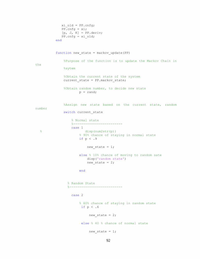
92
xi_old = PP.cnfg; PP.cnfg = xi; [p, J, K] = PP.deriv; PP.cnfg = xi_old; end
function new_state = markov_update(PP)
%Purpose of the function is to update the Markov Chain in
the %sytem
%Obtain the current state of the system current_state = PP.markov_state;
%Obtain random number, to decide new state p = rand;
%Assign new state based on the current state, random
number switch current_state
% Normal state %------------------------- case 1 % disp(num2str(p)) % 90% chance of staying in normal state if p < .9
new_state = 1;
else % 10% chance of moving to random sate disp('random state') new_state = 2;
end
% Random State %---------------------------
case 2
% 60% chance of staying in random state if p < .6
new_state = 2;
else % 40 % chance of normal state
new_state = 1;
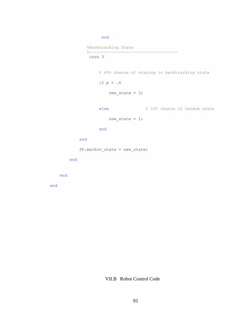
93
end
%Backtracking State %------------------------------------ case 3
% 60% chance of staying in backtracking state
if p < .6
new_state = 3;
else % 10% chance of random state
new_state = 1;
end
end
PP.markov_state = new_state;
end
end
end
VII.B Robot Control Code
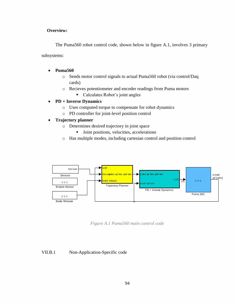
94
Overview:
The Puma560 robot control code, shown below in figure A.1, involves 3 primary
subsystems:
Puma560
o Sends motor control signals to actual Puma560 robot (via control/Daq
cards)
o Recieves potentiometer and encoder readings from Puma motors
Calculates Robot’s joint angles
PD + Inverse Dynamics
o Uses computed torque to compensate for robot dynamics
o PD controller for joint-level position control
Trajectory planner
o Determines desired trajectory in joint space
Joint positions, velocities, accelerations
o Has multiple modes, including cartesian control and position control
Figure A.1 Puma560 main control code
VII.B.1 Non-Application-Specific code
q,qd
Dev ices
brake release
q des qd des qdd des
Trajectory Planner
? ? ?
Puma 560
q des qd des qdd des
q curr qd curr
u [V]
PD + Inverse Dynamics
? ? ?
Enable Motors
Dev ices
Devices
? ? ?
Brake Release
[V]
q [rad]
qd [rad/s]
95
Below is a set of Simulink blocks/subsystems which are not specific to the
applications presented in this thesis, but are rather for general kinematic control of the
robot.
PD + Inverse Dynamics:
This code was written by lab member Andrea Bajo, in 2009
Figure A.2 is a diagram of the PD + Inverse dynamics block. It has 3 general
components
Determining the appropriate control signal
Determining the system dynamics
Converting control signal to voltage
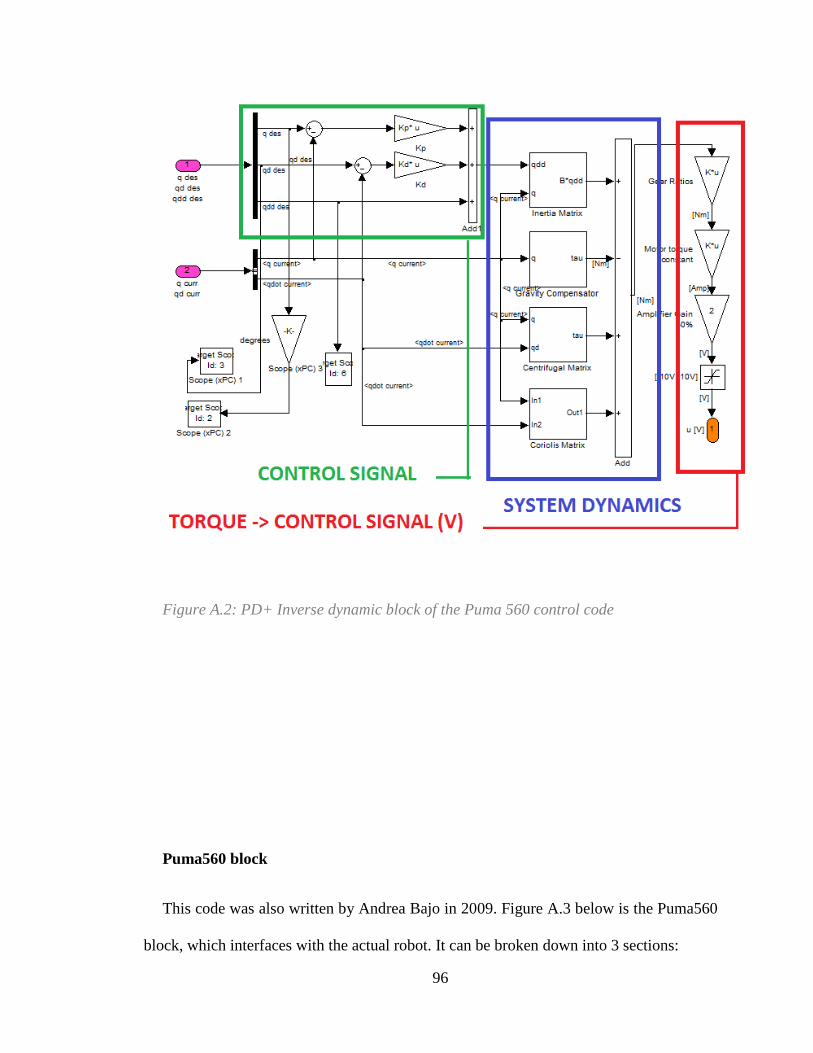
96
Figure A.2: PD+ Inverse dynamic block of the Puma 560 control code
Puma560 block
This code was also written by Andrea Bajo in 2009. Figure A.3 below is the Puma560
block, which interfaces with the actual robot. It can be broken down into 3 sections:

97
Motor signals to robot
Joint signals from robot
Processing Joint signals
Figure A.3: Puma560 Interface subsystem
Trajectory Planner Block
The trajectory planner block switches the Puma between several different
control modes (Cartesian control, Joint Space control, etc..). The code was
designed by Sam Bhattacharyya in 2011, with some original sets of code in the
first two subsystems written by Andrea Bajo and Francesco Senni. The last
subsystem, Mode 4, contains all code used to implement the algorithms presented
in the thesis.
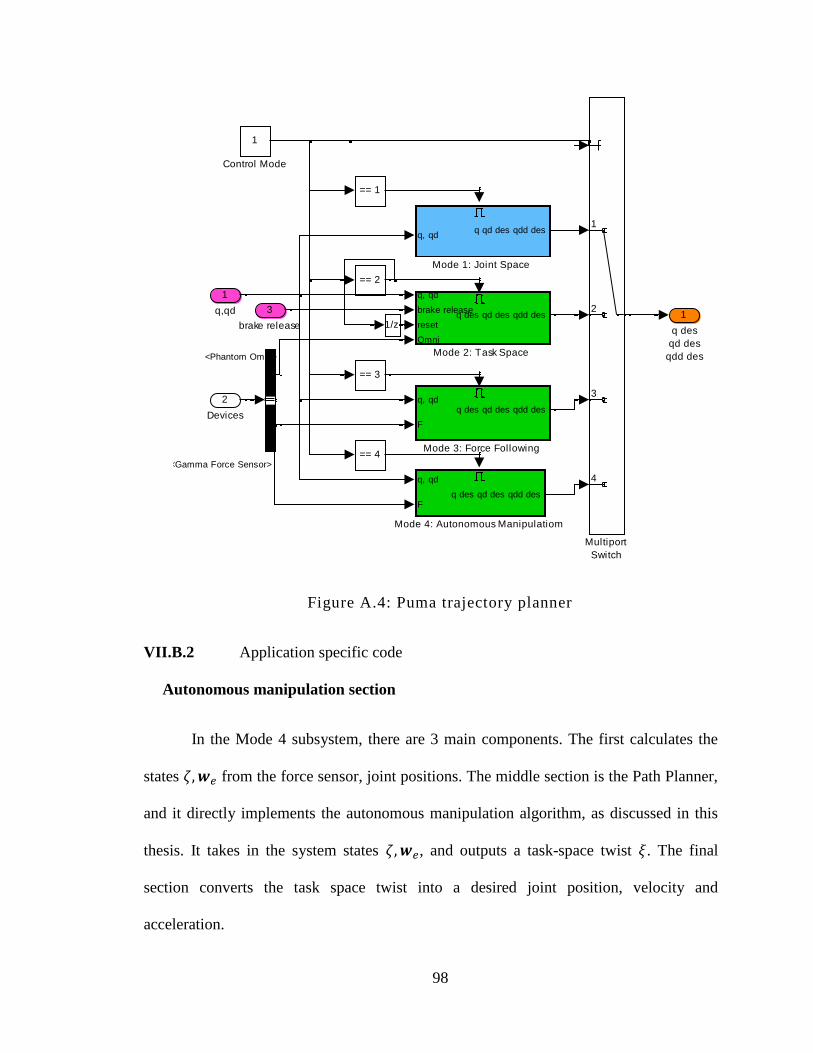
98
Figure A.4: Puma trajectory planner
VII.B.2 Application specific code
Autonomous manipulation section
In the Mode 4 subsystem, there are 3 main components. The first calculates the
states from the force sensor, joint positions. The middle section is the Path Planner,
and it directly implements the autonomous manipulation algorithm, as discussed in this
thesis. It takes in the system states , and outputs a task-space twist . The final
section converts the task space twist into a desired joint position, velocity and
acceleration.
1
q des
qd des
qdd des
1/z
1
2
3
4
Multiport
Switch
q, qd
Fq des qd des qdd des
Mode 4: Autonomous Manipulatiom
q, qd
F
q des qd des qdd des
Mode 3: Force Following
q, qd
brake release
reset
Omni
q des qd des qdd des
Mode 2: Task Space
q, qdq qd des qdd des
Mode 1: Joint Space
1
Control Mode
== 4
== 3
== 2
== 1
3
brake release
2
Devices
1
q,qd
<Phantom Omni>
<Gamma Force Sensor>
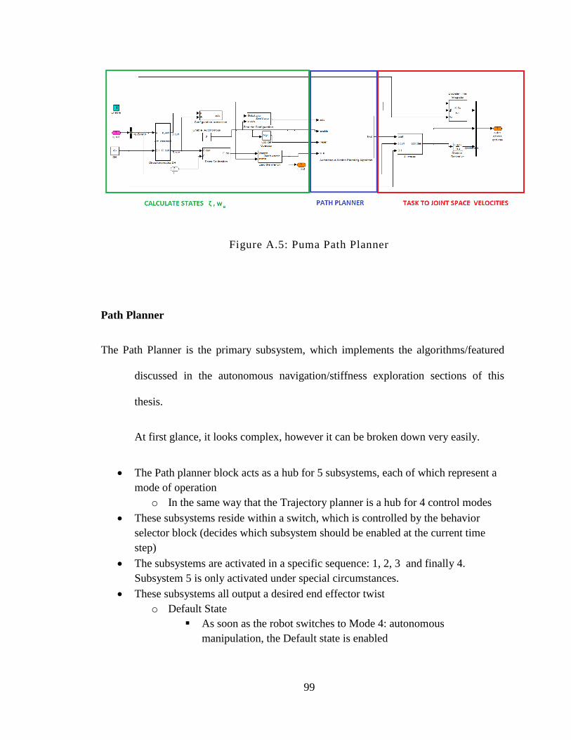
99
Figure A.5: Puma Path Planner
Path Planner
The Path Planner is the primary subsystem, which implements the algorithms/featured
discussed in the autonomous navigation/stiffness exploration sections of this
thesis.
At first glance, it looks complex, however it can be broken down very easily.
The Path planner block acts as a hub for 5 subsystems, each of which represent a
mode of operation
o In the same way that the Trajectory planner is a hub for 4 control modes
These subsystems reside within a switch, which is controlled by the behavior
selector block (decides which subsystem should be enabled at the current time
step)
The subsystems are activated in a specific sequence: 1, 2, 3 and finally 4.
Subsystem 5 is only activated under special circumstances.
These subsystems all output a desired end effector twist
o Default State
As soon as the robot switches to Mode 4: autonomous
manipulation, the Default state is enabled

100
The default state simply output’s a desired manipulator twist of 0,
keeping the robot stationary
o Initialization State
This state simple perturbs the robot along each dimension, and
measures the changes in end effector wrench (to calculate the
initial K)
o Autonomous navigation
Performs the actual path planning code
Is similar to the planar path planning code
o Telemanipulation state
After the robot achieves a given manipulation goal, it switches to
the telemenipulation state, which is also a
Figure A.6: Autonomous navigation Path Planner
1 twistz
1
1
2
3
4
5
Twist Switch
Manual Twist
Telemanipulation
Conf ig
Plot Zeta
Mode
1
2
3
4
5
Mode Selection
Reset
Conf ig
Perturb Twist
Initialization Complete
Wrenches
Initialization Procedure
[CFG]
[WP]
[RF]
[K]
[L]
[W]
[CFG]
From9
[CFG]
[CFG]
[WP]
[RF]
[K]
[CFG]
[L]
[W]
Config
Ko
Mode
K_est
Red F
lags
Safe
Poin
ts
Env explore
Out1
Default
Logic
Constraint
Mode
Behavior Selector
Conf ig
Way Points
Backtrack
Recov ery mode
Backtrack Procedure
Conf ig
K
Red f lags
Auto Twist
Conv ergence
Autonomous Navigation
4
w_e
3
Reset
2
Enable
1
zeta
twist
Logic
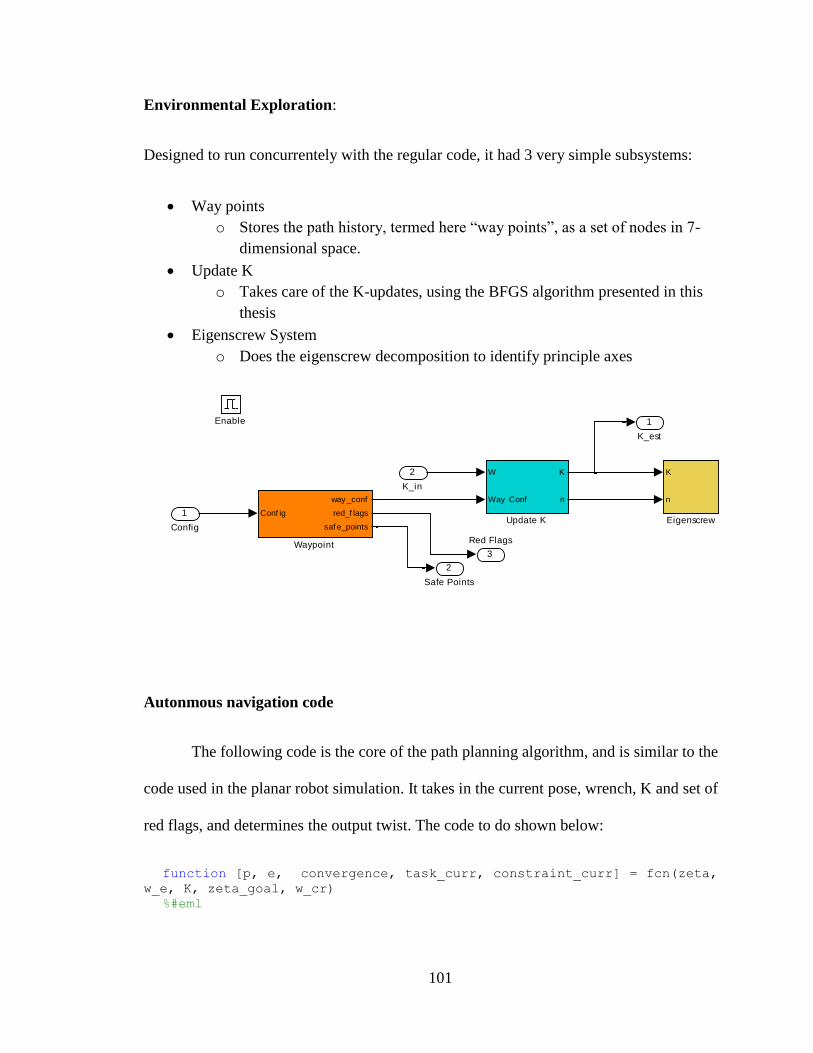
101
Environmental Exploration:
Designed to run concurrentely with the regular code, it had 3 very simple subsystems:
Way points
o Stores the path history, termed here “way points”, as a set of nodes in 7-
dimensional space.
Update K
o Takes care of the K-updates, using the BFGS algorithm presented in this
thesis
Eigenscrew System
o Does the eigenscrew decomposition to identify principle axes
Autonmous navigation code
The following code is the core of the path planning algorithm, and is similar to the
code used in the planar robot simulation. It takes in the current pose, wrench, K and set of
red flags, and determines the output twist. The code to do shown below:
function [p, e, convergence, task_curr, constraint_curr] = fcn(zeta,
w_e, K, zeta_goal, w_cr) %#eml
3
Red Flags
2
Safe Points
1
K_est
Conf ig
way _conf
red_f lags
saf e_points
Waypoint
W
Way Conf
K
n
Update K
K
n
Eigenscrew
Enable
2
K_in
1
Config
102
% Define Initial Constants %------------------------------------------ alpha = .043;
Gamma = diag([1, 1, 0, 0, 0, 0, alpha]);
% Dimensionality weighting matrix % First three entries are in cartesian coord % Last three entries are angular perturbations Gamma_six = diag([1, 1, 1, 5, 5, 5]);
%The curent eps = .005^2;
% 5mm = theoretical perturbation delta = .02; %-----------------------------------------------------
%Calculate the current J value J_curr = task(zeta, zeta_goal, Gamma) + constraint(w_e, w_cr,
Gamma_six, 0); % J_curr = task(zeta, zeta_goal, Gamma);
task_curr = task(zeta, zeta_goal, Gamma); constraint_curr = constraint(w_e, w_cr, Gamma_six, 0);
if task_curr < eps convergence = 1; else
convergence = 0; end
dJ_dx = zeros(6,1);
for i = [1, 2, 6]
%Calculate the hypothetical next move %------------------------------------------- dxi = zeros(6,1); dxi(i,1) = delta; dxi = (Gamma_six)*dxi;
%Calculate the change in each property %------------------------------------------------ dw_e = K*dxi; %Calculate change in wrench
103
dE = w_e.'*dxi; %Calculate change in elastic energy dzeta = proppose(zeta, dxi); %Calculate the change in pose
%Calclate the gradient dJ_dx(i,1) = (task(dzeta, zeta_goal, Gamma) + constraint(w_e + dw_e,
w_cr, Gamma_six, dE) - J_curr)/norm(dxi); % dJ_dx(i,1) = (task(dzeta, zeta_goal, Gamma) - J_curr)/norm(dxi); end
p = -dJ_dx/norm(dJ_dx);
p(4:6,1) = p(4:6,1);
e = distance(zeta, zeta_goal, Gamma);
end
function task = task(zeta, zeta_goal, Gamma)
d = distance(zeta, zeta_goal, Gamma);
task = 1/2*d^2;
end
function d = distance(zeta, zeta_goal, Gamma)
dr = zeta_goal(1:3, 1) - zeta(1:3, 1);
dq = qmult(zeta_goal(4:7).', qinv(zeta(4:7).')).';
dzeta = [dr; dq];

104
d = sqrt(dzeta.'*Gamma*dzeta); d = norm(d - .014);
end
function constraint = constraint(w_e, w_cr, Gamma_six, E)
%Radius of influence roi = .25; %m
%Calculated weighted wrench w_weighted = sqrt(norm((Gamma_six*w_e)));
%Calculate the correct wrench if w_cr < w_weighted constraint = 10^6; else constraint = abs(roi/(w_cr - w_weighted)); end
constraint = constraint + .1*E/w_cr;
end
function dzeta = proppose(zeta, dxi) %The purpose of this function is to propogate the pose, based on the
input infinitessimal displacement given by dxi
%Calculate the angle of displacement th = norm(dxi(4:6,1));
if th == 0 dq = [1, 0, 0, 0];
else % Rotational axis o = (dxi(4:6).')/th;
%Displacement quaternion dq = [cos(th/2), o*sin(th/2)];
end
% Current quaternion qcurr = zeta(4:7)';
% Propogate the current quaternion, by rotation in world frame qprop = qmult(dq, qcurr);
105
rprop = zeta(1:3) + dxi(1:3);
dzeta = [rprop; qprop.'];
end
VII.C Stiffness Code
VII.C.1 Process_K.m
Purpose: The point of this code was to calculate the SPSD approximates of K, and to
then calculate the constraint vectors from those SPSD approximates, using a set of raw
stiffness matrices K. Each K matrix was saved in a different .mat file, obtained directly
from control code.
Associated files: A set of .mat files, no other code needed to function
for i = 1:15
% Load the .mat files load(['Foam_' num2str(i) '.mat'])
% SPSD Approximate %---------------- K_i = (-W)*T^-1;
B = (K_i + K_i.')/2;
[Z, L] = eig(B);
H = Z*L*Z.';

106
K = (B+H)/2; %------------------
% Principle Axis Decomposition %--------------------------- A = K(1:3, 1:3);
B = K(1:3, 4:6);
D = K(4:6, 4:6);
Kv = A;
Kw = D - B.'*A^-1*B; %-------------------------
% Eigenvalues %----------------------- d = abs(eig(Kv));
d = sort(d, 'descend');
r = abs(eig(Kw)); r = sort(r, 'descend');
%Tranlational Tr(:, i) = d';
%Rotational Ro(:, i) = r'; %--------------------------- end
VII.C.2 Particle Filter.m
Purpose: To estimate the optimal classification for a set of constraint vectors
Associated files: clusterfy.m, CU.m
% Particle Filter

107
% The purpose of to classify constraint vectors using clustering,
which is % optimized via particle filtering
clear close all clc
% Load the data load signatures load Locations
% Number of classes k = 2;
% Number of examples E = 15;
% Particle Filter sample size n = 100;
% Classification matrix, each row is the classification for a
particle classification = zeros(n, E);
% Utility vector corresponding to each particle utility = zeros(n,1);
% Load all examples into static variable e = Tr; % Tr from signatures file
% Number of Filters REP = 10;
% Initial random classification %-------------------------------------------------------
for i = 1:n
% Generate a set of random classification
for j = 1:E %For each example, assign a random class classification(i,j) = ceil(rand*k); end end
%---------------------------------------------------------------
108
for reps = 1:REP
for i = 1:n
% Locally optimize each classification
[classification(i,:)] = clusterfy(classification(i,:), e);
utility(i,1) = CU(classification(i,:), e); % % Evaluate the utility of each classification % utility(i,1) = CU(classification(i,:), e);
end
%Randomized elimination %=================================================
norm_factor = max(utility(:,1));
% Probability of elimination pdf = utility(:,1)/norm_factor;
% Elimination vector elimination_vector = zeros(n,1);
for i = 1:n
p = rand;
if pdf(i,1) > p
elimination_vector(i,1) = 1;
end
end
% Replace eliminated variables with new random classifications
for i = 1:n
if elimination_vector(i,1)
for j = 1:E %For each example, assign a random class classification(i,j) = ceil(rand*k); end

109
end end
end
% Graph the results figure(1) hold on
for j = 1:15 % Graph each node
% Decide the color based on it's class %------------------------------------------ clss = optimal(1, j);
switch clss
case 1 clr = 'b';
case 2
clr = 'r'; end %--------------------------------------------
% Plot spcs = [clr 'o']; plot3(e(1,j), e(2,j), e(3,j), spcs, 'MarkerSize', 5, 'LineWidth',
4); end
grid on
VII.C.3 clusterfy.m
110
Purpose: To locally optimize a set of clusters, designed to be operated with a particle
filter, with a set of classifications (particles).
Associated files: Particle_Filter.m
function [classifications, utility] = clusterfy(classification,
examples ) %UNTITLED2 Summary of this function goes here % Detailed explanation goes here
% Number of examples E = length(classification(1,:));
% Number of particles n = length(classification(:, 1));
sse = zeros(n, E);
utility = zeros(n,1);
% For each particle for i = 1:n
% Number of classes k = max(max(classification(i,:)));
% Class count variable clss_cnt = zeros(k,1);
% Average value of each class clss_av = zeros(3, k);
% k lists, one for each class classes = zeros(k, 15);
reor = zeros(k,1);

111
% Locally optimize each particle for t = 1:1
% First, populate the class lists %----------------------------------
for j = 1:E
clss = classification(i, j);
clss_cnt(clss) = clss_cnt(clss) + 1;
classes(clss, clss_cnt(clss)) = j;
end %--------------------------------------
% Find the class average %----------------------------------------- for clss = 1:k
%Clear the class average clss_av(:,clss) = 0;
for j = 1:clss_cnt(clss)
% the current node n, in class i node = classes(clss, j);
%Class average clss_av(:,clss) = clss_av(:,clss) + examples(1:3, node);
end
clss_av(:, clss) = clss_av(:, clss)/clss_cnt(clss);
end
%--------------------------------------------
% Assign each node to new class %--------------------------------------
for j = 1:15
%For the current node
112
%Find best fit, for node to class %------------------------------- for clss = 1:k
v = examples(1:3, j) - clss_av(:,clss);
reor(clss) = v.'*v;
end
[y, clss] = min(reor);
%-------------------------------------
%Re-assign node to class
classification(i,j) = clss;
end
% Examples improved one step for one particle
end
% Examples improved all steps (locally optimized), for one
particle
end
% Examples locally optimized, for all particles
classifications = classification;
end
113
VII.C.4 CU.m
Purpose: To calculate the fitness function for a particular classification of a set of
examples
Associated files: Particle_Filter.m
function [utility] = CU(classification, examples )
% Number of examples E = length(classification(1,:));
% Number of classes k = max(max(classification(1,:)));
% Class count variable clss_cnt = zeros(k,1);
% Average value of each class clss_av = zeros(3, k);
% k lists, one for each class classes = zeros(k, 15);
% First, populate the class lists %----------------------------------
for j = 1:E
clss = classification(1, j);
114
clss_cnt(clss) = clss_cnt(clss) + 1;
classes(clss, clss_cnt(clss)) = j;
end %--------------------------------------
% Find the class average %----------------------------------------- for clss = 1:k
%Clear the class average clss_av(:,clss) = 0;
for j = 1:clss_cnt(clss)
% the current node n, in class i node = classes(clss, j);
%Class average clss_av(:,clss) = clss_av(:,clss) + examples(1:3, node);
end
clss_av(:, clss) = clss_av(:, clss)/clss_cnt(clss);
end %--------------------------------------------
% Find the sum of squared error %--------------------------------------
sse = 0;
for j= 1:15
clss = classification(1,j);
v = examples(1:3, j) - clss_av(:, clss);
sse = sse + v.'*v;
end
%------------------------------------------ utility = sse;
end

115
VIII Appendix B: Hardware
VIII.A Gripper
VIII.A.1 Gripper version 1.0
In order to manipulate objects and evaluate stiffness, some type of gripper needs
to be mounted on top of the ATI Gamma Force sensor. The image below shows the Pro-
Engineer model for a custom gripper, developed by Sam Bhattacharyya in June 2011,
including an attachment to the force sensor.
This gripper is actuated by a large push style solenoid, McMaster Part# 69905K48,
and the solenoid is housed within the large cylindrical portion of the gripper. The
solenoid has a stroke of approximately 20mm while assembled within the gripper, and the
gripper is able to grip down with a force of ~10 N.
The gripper is almost entirely manufactured out of ABS, via rapid prototyping.
The associated files are available at arma.vuse.vanderbilt.edu/mediawiki
Figure A.8: Puma Gripper Pro-E model, V 1.0

116
Electronics setup for gripper + relay
The solenoid is a simple on/off mechanism that pushes/extends a rod outwards when a
specified voltage, at high enough current, applied across the solenoid’s leads (polarity
doesn’t actually matter). The resulting control circuit is actually quite simple, and is
detailed in the image to the right.
Below is a table including the parts used in the electronic setup, which were ordered
from OnlineComponents.com
Part number Description
1-1393788-6 5V 5A Relay
2N3392 NPN Transistor
1.5KE100CA/54 Diode
RL020S222G Resistor
These components were organized into the following circuit
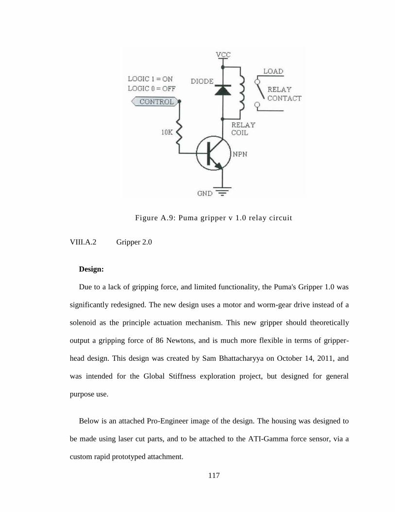
117
Figure A.9: Puma gripper v 1.0 relay circuit
VIII.A.2 Gripper 2.0
Design:
Due to a lack of gripping force, and limited functionality, the Puma's Gripper 1.0 was
significantly redesigned. The new design uses a motor and worm-gear drive instead of a
solenoid as the principle actuation mechanism. This new gripper should theoretically
output a gripping force of 86 Newtons, and is much more flexible in terms of gripper-
head design. This design was created by Sam Bhattacharyya on October 14, 2011, and
was intended for the Global Stiffness exploration project, but designed for general
purpose use.
Below is an attached Pro-Engineer image of the design. The housing was designed to
be made using laser cut parts, and to be attached to the ATI-Gamma force sensor, via a
custom rapid prototyped attachment.

118
Figure A.10: Puma gripper v 2.0 Pro-Engineer model
Specifications
Overview
Gripping Force: 86.4 N
Actuation time: 1.375 s
Weight: .8824 kg
Center of Grip: 185 mm along Force sensor Z axis
Force analysis
Motor specifications for Pololu 29:1 Metal Gear Motor
Operating Voltage: 6V
Free run speed: 440 rpm
Stall Current: 3.3 Amps
Stall Torque: .18Nm
Transmission Specification (Worm drive x1)
Gear ratio: 60:1
Worm Gear SDP-SI Part # A 1B 6MYH08R060
o Module: .80
o # of Teeth: 60
o Gear Ratio: 60:1
o Pitch Diameter: 48.00 mm

119
Worm SDP-SI Part # A 1Y 5MYK08RA
o Module: .8
o Pitch diameter: 10.4mm
o Leads: 1
o Hub Configuration: 5mm bore, with set screw
End effector Specification
Lever arm: 75 mm
Range of motion: 0 - 65 mm
Angular range of motion:0 - 110 degrees (between arms), 0 - 55 degrees per arm
Gripper force: 86.4 N
o Force = [(Lever Arm)^-1]*[(Motor Torque)*(Gear Ratio)*(Gear
Efficiency)]
o Force = (.075 m)^-1*(.18 Nm)*(60)*(.6)
Actuation time: 1.375 seconds
o Angular Speed = (Motor Speed)*(Speed Efficiency @ No load)*(Gear
Ratio)^-1
o Angular Speed = 40 deg/s = 6.6 rpm = (400 rpm)*(90%)*(60)^-1
o Actuation time = (Angular range of motion)/(Angular speed)
Weight:
The approximate weight of the gripper is .8843 kg, numerically calculated from
the Pro-Engineer model. With respect to the coordinate frame of the ATI Gamma Force
sensor, via the specified attachment block, the center of gravity of the Gripper is located
in the table below:
Coordi
nate
Distance
X 0 mm
Y -
9.003mm
Z 100.005
mm
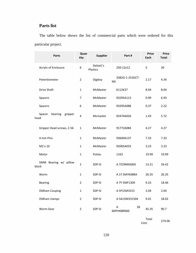
120
Parts list
The table below shows the list of commercial parts which were ordered for this
particular project.
Parts Quan
tity Supplier Part #
Price Each
Price Total
Acrylic of Enclosure 6 Delvie\'s
Plastics 250-12x12 5 30
Potentiometer 2 Digikey 3382G-1-253GCT-
ND 2.17 4.34
Drive Shaft 1 McMaster 6112K37 8.04 8.04
Spacers 7 McMaster 93295A113 0.99 6.93
Spacers 6 McMaster 93295A088 0.37 2.22
Spacer bearing gripper head
4 Mcmaster 92474A026 1.43 5.72
Gripper Head screws, 2-56 1 McMaster 91772A084 4.27 4.27
4 mm Pins 1 McMaster 93600A137 7.33 7.33
M2 x 10 1 McMaster 92005A033 3.23 3.23
Motor 1 Pololu 1163 19.99 19.99
5MM Bearing w/ pillow block
2 SDP-SI A 7Z29MXS005 13.21 26.42
Worm 1 SDP-SI A 1Y 5MYK08RA 26.35 26.35
Bearing 2 SDP-SI A 7Y 5MF1304 9.23 18.46
Oldham Couping 1 SDP-SI A 5P15M3315 2.04 2.04
Oldham clamps 2 SDP-SI A 5A15M331504 9.01 18.02
Worm Gear 2 SDP-SI A 1B
6MYH08R060 45.35 90.7
Total Cost:
274.06

121
VIII.B Experimental Setup
VIII.B.1 Rigid triangle Experiment
The main structure of the rigid triangle experiment was created via laser cutting of
¼’’ acrylic sheets of plastic.
Figure A.11: Rigid triangle fully setup, with spring
Two primary pieces were cut out of acrylic: The frame itself (below, left), and the
rigid triangle (below, right).
Figure A.12: The rigid triangle experiment setup -components

122
The length of the side of each triangle is , the length of the laser cut frame
was 1 ftx1ft, with a thickness a border thickness of 1’’.
The springs used were simple linear 1kN/m springs, McMaster Part number
9654K125. The unstreched length of each spring was 31.75mm, and there were two
springs, hooked in series, between each vertex of the triangle, and it’s fixed location on
the environment.
Related Documents


![4MDS: A GEOMETRIC CONSTRAINT BASED MOTION DESIGN … · Design Simulation Technologies [34] and other synthesis tools found in earlier versions of the text. ... ulate the motion of](https://static.cupdf.com/doc/110x72/5b5e47197f8b9a057e8be26c/4mds-a-geometric-constraint-based-motion-design-design-simulation-technologies.jpg)