Fys-3921 Master’s Thesis in Electrical Engineering Motion induced electromagnetic fields in the ocean: Exploratory data analysis and signal processing by Andreas Eide Supervisors: Alfred Hanssen and Mårten Blixt December, 2007 Faculty of Science Department of Physics and Technology University of Tromsø

Welcome message from author
This document is posted to help you gain knowledge. Please leave a comment to let me know what you think about it! Share it to your friends and learn new things together.
Transcript
Fys-3921Master’s Thesis in Electrical Engineering
Motion induced electromagneticfields in the ocean: Exploratory
data analysis and signal processing
by
Andreas Eide
Supervisors: Alfred Hanssen and Mårten Blixt
December, 2007
Faculty of Science
Department of Physics and TechnologyUniversity of Tromsø

Abstract
We will in this thesis analyse data from antennas located at the seafloor mea-suring the vertical component of the natural electric field. The internal sourceto electromagnetic fields in the ocean is saltwater crossing the geomagneticfield, and the main contributor to the motion induced vertical electric field isthe water velocity in the East-West direction weighted by the North compo-nent of the geomagnetic field. The motivation is to study the motion inducedsignal which is present in the frequency range 0.1-10 Hz. This is a frequencyrange of interest when using electromagnetic methods in marine hydorcar-bon exploration.
To analyse the electric field data we have implemented and applied the mul-titaper estimator for spectrum estimation. The multitaper estimator also pro-vide for a test for periodic (sinusoidal) components, which we have imple-mented and applied. To further analyse the statistics of the motion inducedelectric field, we have applied both conventional estimators to estimate thestatistical properties and the kernel smoothing estimator to estimate the dis-tribution of the data.
The electric field data contained a prominent oscillation visible in the timeseries, and the spectrum estimates of the recorded data show a prominentpeak about 0.15 Hz and with features just above 0.1 Hz and at 0.24 Hz. Thesefeatures corresponds to the observed periods of the surface waves during therecordings. While the frequency of the prominent peak is rather stable, itslevel changes more than 10 dB during the recording (30 minutes). Theoryand other experiments shows that the surface waves causes pressure fluctua-tion in the ocean, causing both disturbance in the seafloor and the seawater,which induce electric fields. This mechanism is the most likely source to thefluctuations we see in the measured data.
i

Acknowledgements
I thank Alfred Hanssen for his excellent work as supervisor during the study,particularly for sharing his knowledge about data analysis and for all the help-ful discussions and comments about the manuscript.
The assignment was proposed by Mårten Blixt at Discover Petroleum, whichalso provided the data sets from the electric field and the antenna positionmeasurements. I thank him for his excellent work as supervisor, and for use-ful comments and discussions about electromagnetism and the manuscript.I also thank Tom Grydeland at Discover Petroleum for useful comments to themanuscript, and I thank Discover Petroleum in general for sharing their data.
I also thank the helpful people both at Tromsø Geophysical Observatory, Uni-versity of Tromsø, Norway for providing the geomagnetic data, and Meterol-ogisk Institutt (www.met.no) for providing the weather (ocean) data. I alsothank Jonathan Lilly (Earth and Space Research, Seattle) for the useful inputson the ocean wave dynamics.
iii


Contents
Abstract i
Acknowledgements iii
Contents v
1 Introduction 1
2 Electromagnetic induction in the ocean 52.1 Maxwell equations . . . . . . . . . . . . . . . . . . . . . . . . . . . . . . . . . 52.2 Conductivity . . . . . . . . . . . . . . . . . . . . . . . . . . . . . . . . . . . . . 72.3 Motion induced electric fields . . . . . . . . . . . . . . . . . . . . . . . . 72.4 The vertical electric field . . . . . . . . . . . . . . . . . . . . . . . . . . . . 82.5 Induction in antenna . . . . . . . . . . . . . . . . . . . . . . . . . . . . . . . 112.6 Noise sources . . . . . . . . . . . . . . . . . . . . . . . . . . . . . . . . . . . . 12
2.6.1 Surface waves induced noise . . . . . . . . . . . . . . . . . . . . 122.6.2 Turbulent Eddies . . . . . . . . . . . . . . . . . . . . . . . . . . . . 132.6.3 Other noise sources . . . . . . . . . . . . . . . . . . . . . . . . . . 13
3 Experiment 153.1 Electric field measurements . . . . . . . . . . . . . . . . . . . . . . . . . . 153.2 Measurements of antenna motion . . . . . . . . . . . . . . . . . . . . . 17
4 Signal analysis and processing methods 194.1 Statistical properties . . . . . . . . . . . . . . . . . . . . . . . . . . . . . . . 20
4.1.1 Sample moments . . . . . . . . . . . . . . . . . . . . . . . . . . . . 214.2 Estimation of the probability density . . . . . . . . . . . . . . . . . . . 21
4.2.1 Histogram . . . . . . . . . . . . . . . . . . . . . . . . . . . . . . . . . 224.2.2 Parzen window estimator . . . . . . . . . . . . . . . . . . . . . . 22
4.3 Stationarity . . . . . . . . . . . . . . . . . . . . . . . . . . . . . . . . . . . . . . 234.3.1 Runs Test . . . . . . . . . . . . . . . . . . . . . . . . . . . . . . . . . . 24
4.4 Power spectrum estimation . . . . . . . . . . . . . . . . . . . . . . . . . . 25
v

vi CONTENTS
4.4.1 Definition of the power spectrum density . . . . . . . . . . 254.4.2 Basic power spectrum estimators . . . . . . . . . . . . . . . . 26
4.5 Multitaper power spectrum estimation . . . . . . . . . . . . . . . . . . 294.5.1 Selecting the optimal window functions - discrete pro-
late spheroidal sequences . . . . . . . . . . . . . . . . . . . . . . 294.5.2 The multitaper estimator . . . . . . . . . . . . . . . . . . . . . . 35
4.6 The chi-square and F -distributions . . . . . . . . . . . . . . . . . . . . 424.6.1 The chi-square distribution . . . . . . . . . . . . . . . . . . . . . 424.6.2 The F -distribution . . . . . . . . . . . . . . . . . . . . . . . . . . . 44
4.7 Distribution of spectrum estimates . . . . . . . . . . . . . . . . . . . . . 464.8 Confidence interval of the multitaper spectral estimate . . . . . . 484.9 Thomson’s F -test for single frequency components . . . . . . . . . 49
4.9.1 Numerical example . . . . . . . . . . . . . . . . . . . . . . . . . . . 51
5 Results 535.1 E-field measurements: 50 m cable antenna, Station 1 . . . . . . . 53
5.1.1 Time series . . . . . . . . . . . . . . . . . . . . . . . . . . . . . . . . . 535.1.2 E-field runs test . . . . . . . . . . . . . . . . . . . . . . . . . . . . . 545.1.3 Multitaper estimation, number of averaged eigenspectra 555.1.4 Time series, spectral estimates and probability density
function estimates . . . . . . . . . . . . . . . . . . . . . . . . . . . 575.1.5 Approximate slope of the background spectrum . . . . . . 655.1.6 F -test for sinusoidal components . . . . . . . . . . . . . . . . 665.1.7 Time development of the prominent peak . . . . . . . . . . 72
5.2 Measurements of antenna position . . . . . . . . . . . . . . . . . . . . 765.3 Geomagnetic activity . . . . . . . . . . . . . . . . . . . . . . . . . . . . . . . 795.4 E-field measurements from other locations . . . . . . . . . . . . . . . 81
6 Discussion and conclusions 85
Bibliography 89
Chapter 1
Introduction
For marine hydrocarbon (oil/gas) exploration, the most important tool forsubsurface imaging is without doubt the seismic reflection method. In seis-mics, a pressure wave is launched close to the sea surface that reflects at inter-faces between formations of different acoustic impedance. By measuring thetime it takes for the wave to return to a receiver, a map of the seafloor and thesediments can be retrieved (e.g., Dobrin and Savit [1988]). However, withinthe last decade, an increasingly important method, named Controlled-SourceElectromagnetic (CSEM) method, has appeared (MacGregor and Sinha [2000],Ellingsrud et al. [2002], Eidesmo et al. [2002], Kong et al. [2002], Johansen et al.[2005]). In contrast to seismics, the information in the CSEM method is prop-agated by the diffusion of electromagnetic energy, and has a resolution pro-portional to the depth of the target, which is much worse than for seismicmethods (e.g., Constable and Srnka [2007]). However, the CSEM method isdirectly sensitive to the electric resistivity of the sediments, and the resistiv-ity in hydrocarbon filled sediments is substantially higher than for sedimentsfilled with saltwater. Therefore, the CSEM methods can be used to map the re-sistivity of the sediments, and hence provide a direct measure of the existenceof hydrocarbons in the sediments. Academic research on marine electromag-netic methods for analysing the solid Earth beneath the ocean has been quiteactive since the 70’s, and Chave et al. [1991] presents several of the devel-oped methods. It was not until Ellingsrud et al. [2002] and Eidesmo et al.[2002] showed that the method was sensitive enough to detect thin hydrocar-bon reservoirs that it caught interest in the hydrocarbon exploration industry.In Norway, Petromarker and EMGS have patented their own CSEM methods,called "Petromarker" and "Sea Bed Logging", respectively.
As an oceanographic tool the electromagnetic methods provide useful mea-sures of ocean currents. Because the marin environment is conductive, any
1
2 CHAPTER 1. INTRODUCTION
motion, of the water or of the receiving antennas, will create an electromag-netic force in the Earths magnetic field. The internal source of electromag-netic fields in the ocean is saltwater moving across the geomagnetic field, andparticles with opposite charge will due to the Lorentz force be separated intoopposite directions and build up an electric field across a seawater stream.By measuring the cross stream voltage, this can be used to monitor oceanstreams in terms of velocity, and e.g., Chave and Filloux [1985] and Bind-off et al. [1986], present experiments where the vertical electric field wereused as a measure of the long-term East-West water velocity. Larsen [1992]presents a thorough research from the Strait of Florida, where the horizontalcross stream voltage have been measured since 1969 by a long sub sea cable(abandoned communications cable). For a bounded stream through a strait,the velocity can hence be related to the volume transport through the strait.Because of lateral changes in a strait boundaries and inhomogeneous watervelocity, there will also be potential difference along the stream boundaries.Harvey and Montaner [1977], Palshin et al. [2002] and Palshin et al. [2006]present experiments, were the voltage along the stream were measured by on-land receivers directed almost parallel to the ocean stream, that give a mea-sure of the tide.
For the CSEM method, any motion induced electric field will appear as anunwanted source of noise. Roughly, it can be expressed as a part of the totalmeasured field as, EMEAS = ECSEM + ESW + Eother. Here, ECSEM is related to thefield from the CSEM transceiver, ESW is the motion induced field, and Eother iscaused by other noise sources, like distortion from the geomagnetic field andnoise from the electrodes and electronics. A further complication is that thefluctuation in the electric field at the seafloor is related to the surface waves(Cox et al. [1978], Webb and Cox [1986]), which coincide with important fre-quencies used in CSEM. The motivation is thus to reduce the effect of ESW ,and the presented methods and analysis will be useful for further analysis ofthe motion induced field.
We will in this thesis present measured data of the vertical component of themotion induced electric field, recorded by a vertical antenna placed at theseafloor. During the recordings, the position of the antenna was also moni-tored to reveal relations between the motion of the antenna and the recordedelectric field. Unfortunately, because of the lack of accuracy in the positiondata, we can not tell if the observed motion were the actual motion of theantenna, or an effect of uncertainties in the measurement. We will thereforefocus on analysing the electric field data. The frequency range of interest is0.1-10 Hz, and observations of the vertical electric field in this frequency range
3
are limited.
To analyse the electric field data, we will present some advanced data anal-ysis methods in great detail, in particular the multitaper spectrum estima-tor (Thomson [1982]), which has good variance properties, also for relativelyshort data segments. By the use of the multitaper method we can also ex-tend the spectrum analysis with an F -test to search for single frequency com-ponents (proposed by Thomson [1982], example of implementation by Lees[1995]). We have implemented an automatic version of the F -test which willbe applied. To further analyse the statistics of the motion induced electricfield, we will apply both conventional estimators to estimate the statisticalproperties, and also apply a more advanced kernel smoothing estimator ofthe probability density function (e.g., Silverman [1986]).
In Chapter 2 we will describe the electromagnetic properties of the ocean, thevertical electric field in particular and noise sources. The measurement setupis described in Chapter 3. In Chapter 4 we present the analysis methods, andthe multitaper spectrum estimator in particular. We then apply the methodsto the real data, and the results are presented in Chapter 5. The methods andresults are discussed in Chapter 6, which also contains the conclusions.


Chapter 2
Electromagnetic induction in theocean
In this chapter we will describe some of the electromagnetic properties of theocean. We will derive an approximation of the electric field measured by a ver-tical antenna, and describe the dominant internal noise sources that generatefluctuation in the electric field between 0.1−10 Hz.
2.1 Maxwell equations
For electromagnetic fields at low frequency in the conducting ocean and seabed,the conductive electric currents are dominant, and Maxwell’s equations sim-plifies to (e.g., Larsen [1973])
∇·D=q (2.1)
∇·B= 0 (2.2)
∇×E=−∂ B
∂ t(2.3)
∇×B=µJ. (2.4)
Here, B is the magnetic induction (W b/m 2), E the electric field (V /m ), D isthe electric displacement (C/m 2), J is the electric current density (A/m 2), andq is the electric charge density, C/m 3. The magnetic permeability µ is equalto µ0 = 4π×10−7(H/m ) (e.g., Keller [1987]).
Ohm’s law for a moving conducting medium with fluid particle velocity v (m/s)and conductivityσ (Ωm)−1 is given by (e.g., Sanford [1971])
J=σ(E+v×B). (2.5)
5
6 CHAPTER 2. ELECTROMAGNETIC INDUCTION IN THE OCEAN
When taking the curl of Eq. (2.3) and inserting (2.4), the differential equationfor E can be derived as
∇×∇×E=− ∂∂ t(∇×B) (2.6)
∇(∇·E)−∇2E=−µ0∂
∂ t(J). (2.7)
For simplicity we assume zero velocity of the water, v = 0, and Ohm’s law be-comes J=σE. In addition we assume∇· J= 0. The leftmost part in (2.7) thenbecomes zero,
∇(∇·E) =∇(∇· J/σ) = 0, (2.8)
and when inserting J=σE into the right side of Eq. (2.7), we get
−∇2E=−µ0σ∂
∂ t(E) =>
∂ E
∂ t− 1
µ0σ∇2E= 0. (2.9)
This equation can be recognised as the diffusion equation
∂ E
∂ t−D∇2E= 0, (2.10)
where the diffusion coefficient is D = 1/µ0σ. As we can see the diffusion de-pends on the conductivity, which is an important property for electromag-netic exploration. When e.g., an electric field is set up by a transceiver andthen turned off, the decay rate of the electric field measured by a distancedreceiver can be used to map the conductivity in the sediments between thetransceiver and the receiver, and areas with high resistivity (low conductivity)can be detected.
The skin depth δs is an important parameter both for how deep external elec-tromagnetic fields (geomagnetic) penetrate into the ocean, and for how deepan electromagnetic field set up by a CSEM transceiver penetrate into the sed-iments. It represent the distance an electromagnetic wave diffuse into a con-ducting medium, and where the amplitude is e−1 of its initial value (e.g., Fil-loux [1973])
δs =
r1
π f µ0σ. (2.11)
Here, f is the frequency of the electromagnetic field, andσ is the conductivityof the medium.
It should be mentioned that Løseth et al. [2006] reviewed the theory of EM

2.2. CONDUCTIVITY 7
fields propagating in the conducting ocean, and concluded that the approx-imation leading to a diffusion equation is valid, but that mathematically it ismore correct to express it as wave propagation with dispersion and attenua-tion.
2.2 Conductivity
The ocean conductivity depends mostly on temperature and salinity, and canbe approximated as (e.g., Chave et al. [1991]),
σ(T ) = 3+T /10. (2.12)
Here, T is given in Celsius, and T /10 is the approximation of the contributionfrom the salinity. For the sediments, the conductivity can be modelled withArchie’s law (e.g., Keller [1987])
σ= aσWφm , (2.13)
where φ is the porosity of the rock, σW is the conductivity of the pore water.Here, a and m are fitting parameters for different rock types which are foundexperimentally. Some of the pores can be occupied by hydrocarbons (oil/gas)with low conductivity, replacing the conductive water, and the conductivity ofthe rock can then be written as
σ= aσW (1−SHC )nφm , (2.14)
where SHC is the saturation of hydrocarbons, andφ is the porosity of the rock,and n the saturation factor. As we can see from latter equation, the conduc-tivity of the rock will decrease if saturated by hydrocarbons, and increase itselectric resistivity.
2.3 Motion induced electric fields
Following Sanford [1971], we assume the electric field to be quasi-static. Thismeans that ∇×E= 0, and a scalar electric potential φ exists (E=−∇φ). Withthis approximation, the time variations of the magnetic induction is neglected,and the contribution from the magnetic field is only due to the static geomag-netic field, F. If we rearrange Eq. (2.5), and replace B with F, we get
E= J/σ−v×F. (2.15)
A stationary receiver will experience particle motion at the same velocity asthe water velocity, and Eq. (2.15) is a good approximation of the measured

8 CHAPTER 2. ELECTROMAGNETIC INDUCTION IN THE OCEAN
electric field when using a receiver fixed to the sea floor (e.g., Sanford [1971],Filloux [1973]).
For a receiver drifting along with the water velocity, the water motion seenfrom the receiver is zero, and the measured electric field is given by (Filloux[1973])
E= J/σ (2.16)
For a vertical receiver, one electrode is fixed at the seafloor and the other heldup by a buoy. The buoy will drift with the water stream until a balance withthe buoy up drift and the cable tension is reached. In this position the cablebetween the electrode and the buoy will partly move with the water. The ap-parent velocity seen from the receiver will therefore be a combination of thewater motion and the motion of the receiver.
2.4 The vertical electric field
Figure 2.1: Simple model of a two layered earth, with a conductive ocean over a layerof conductive sediments. The layers are isolated by non-conductive air and crust. Avertical receiver is fixed to the sea floor in the middle of the figure.
2.4. THE VERTICAL ELECTRIC FIELD 9
We now assume a wide laminar ocean stream with a homogeneous velocityin either north-south or east-west direction. To calculate the electric field weuse typical values of the static earth magnetic field at a high latitude. We ne-glect the contribution from sea surface waves and sea floor topographic, andassume a flat sea surface and sea floor. The model is placed in a Cartesian co-ordinate system, with x to East, y to North and z upwards, with the respectiveunit vectors i, j and k (see figure 2.1).
First we look at the contribution from v×F and neglect the part containingthe current density (J/σ), to obtain
E=−v×F= (vz Fy −vy Fz )i+(vx Fz −vz Fx )j+(vy Fx −vx Fy )k. (2.17)
A vertical antenna will only detect the vertical component, which has an am-plitude of (vy Fx − vx Fy ). The time varying geomagnetic field is assumed to besmall, and the E-field as a function of time, can be approximated as
Ez (t ) = vy (t )Fx −vx (t )Fy . (2.18)
We now see that changes in the local horizontal water velocity v, will actuallyinduce an vertical electric field. Since Fx and Fy are the horizontal compo-nents of the static geomagnetic field, the vertical electric field gives a measureof the water velocity in the geomagnetic East-West direction.
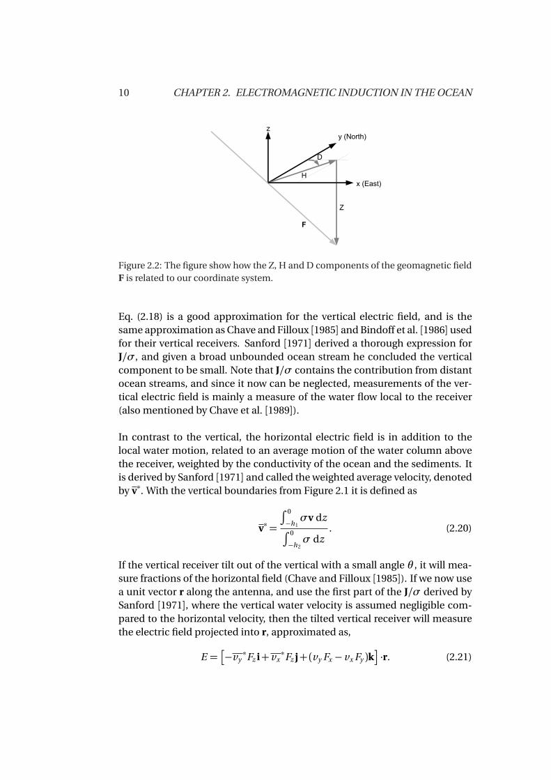
On-land magnetometers normally measure the geomagnetic field in a verti-cal component Z , a horizontal component H , and a declination D given indegrees east of North. Figure 2.2 place these components in our coordinatesystem, giving Fx = H sin(D) and Fy = H cos(D). The declination D is nor-mally small, but its value depends on the location, but will in general increaseat high latitudes. The electric field data presented in this thesis, were recordedat about 61°North. If we use the values from the nearest magnetometer sta-tion (Solund, 61°N, Tromsø Geophysical Observatory [2007]), it shows a typ-ical declination of D = −1.2. This gives |Fy /Fx | = 1/tan(D) ≈ 50, and for ourlocation the main contributor to the vertical E-field is the water velocity inthe latitudinal (zonal) East-West direction, weighted by the horizontal Northcomponent of the geomagnetic field
Ez (t )≈−vx (t )Fy . (2.19)
A typical ocean stream is in the range 1 m/s or less (Sanford [1971]). Again,we use the typical geomagnetic field from Solund (61°N, Tromsø GeophysicalObservatory [2007]), and for a ocean velocity of 1 m/s in the East-West direc-tion, the vertical electric field would be
|Ez |= 1 m/s ·14500 nT · cos(1.2)≈ 14.5 µV/m.
10 CHAPTER 2. ELECTROMAGNETIC INDUCTION IN THE OCEAN
Figure 2.2: The figure show how the Z, H and D components of the geomagnetic fieldF is related to our coordinate system.
Eq. (2.18) is a good approximation for the vertical electric field, and is thesame approximation as Chave and Filloux [1985] and Bindoff et al. [1986] usedfor their vertical receivers. Sanford [1971] derived a thorough expression forJ/σ, and given a broad unbounded ocean stream he concluded the verticalcomponent to be small. Note that J/σ contains the contribution from distantocean streams, and since it now can be neglected, measurements of the ver-tical electric field is mainly a measure of the water flow local to the receiver(also mentioned by Chave et al. [1989]).
In contrast to the vertical, the horizontal electric field is in addition to thelocal water motion, related to an average motion of the water column abovethe receiver, weighted by the conductivity of the ocean and the sediments. Itis derived by Sanford [1971] and called the weighted average velocity, denotedby v∗. With the vertical boundaries from Figure 2.1 it is defined as
v∗ =
∫ 0
−h1σv dz
∫ 0
−h2σ dz
. (2.20)
If the vertical receiver tilt out of the vertical with a small angle θ , it will mea-sure fractions of the horizontal field (Chave and Filloux [1985]). If we now usea unit vector r along the antenna, and use the first part of the J/σ derived bySanford [1971], where the vertical water velocity is assumed negligible com-pared to the horizontal velocity, then the tilted vertical receiver will measurethe electric field projected into r, approximated as,
E =−vy
∗Fz i+vx∗Fz j+(vy Fx −vx Fy )k
·r. (2.21)
2.5. INDUCTION IN ANTENNA 11
2.5 Induction in antenna
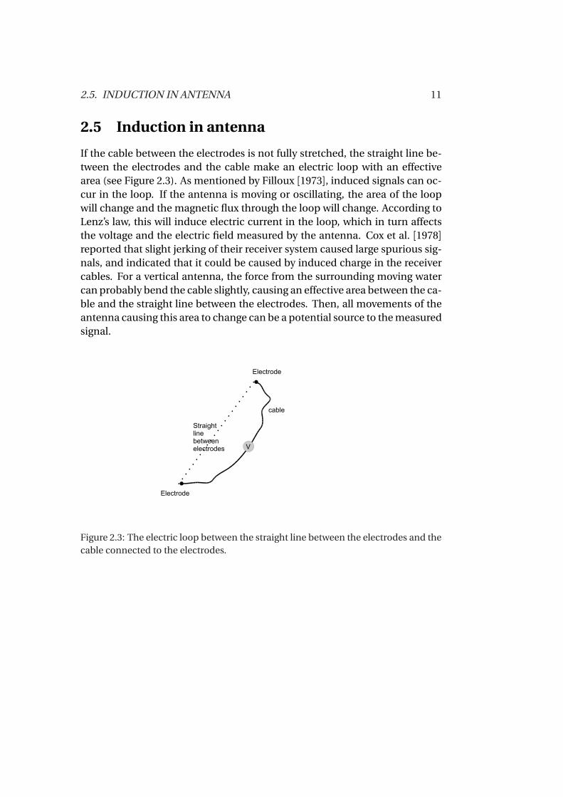
If the cable between the electrodes is not fully stretched, the straight line be-tween the electrodes and the cable make an electric loop with an effectivearea (see Figure 2.3). As mentioned by Filloux [1973], induced signals can oc-cur in the loop. If the antenna is moving or oscillating, the area of the loopwill change and the magnetic flux through the loop will change. According toLenz’s law, this will induce electric current in the loop, which in turn affectsthe voltage and the electric field measured by the antenna. Cox et al. [1978]reported that slight jerking of their receiver system caused large spurious sig-nals, and indicated that it could be caused by induced charge in the receivercables. For a vertical antenna, the force from the surrounding moving watercan probably bend the cable slightly, causing an effective area between the ca-ble and the straight line between the electrodes. Then, all movements of theantenna causing this area to change can be a potential source to the measuredsignal.
Figure 2.3: The electric loop between the straight line between the electrodes and thecable connected to the electrodes.
12 CHAPTER 2. ELECTROMAGNETIC INDUCTION IN THE OCEAN
2.6 Noise sources
2.6.1 Surface waves induced noise
Cox et al. [1978] investigated the electromagnetic signature generated by swellwith a period of the dominant wave, T ≈ 10 s. Electromagnetic fields gen-erated at the sea surface, will have the same frequency as the surface wave,f = 1/T ≈ 0.1 Hz. The ocean skin depth for this frequency will be δs =p
1/π f µ0σ ≈p
1/(π ·0.1 ·4π×10−7 ·3.3) ≈ 870 m, where the ocean conduc-tivity is assumed to be σ = 3.3 (Ωm)−1 (from Larsen [1973]). Electromagneticfields propagating this distance of ocean depth will be strongly attenuated,and with a strength of swell generated magnetic field at the sea surface b ¯ 10nT (from Lilley et al. [2004]), the propagating electromagnetic field will defi-nitely decay to undetectable levels below the skin depth. Still, the electromag-netic signature related to swell are strong also at greater depths.
Theory derived by Longuet-Higgins [1950] show that when surface waves fromdifferent directions interacts, they generate pressure oscillations in the un-derlying ocean. Surface waves from opposite directions of approximately thesame wavelength and phase will form standing waves twice per wave periodwhen they interact head on, and the oscillations will be around twice the swellfrequency. The pressure fluctuations will propagate through the ocean, andwhen reaching the solid ocean floor, it may generate small motions in thesea floor and cause small scale quake disturbances, called microseism. In theocean, spatial differences in the pressure may set up ocean streams, which inturn induce electromagnetic fields (Cox et al. [1978]).
Cox et al. [1978]measured the horizontal electric field with a receiver fixed tothe seafloor at depths greater than the electromagnetic skin depth (1.2 to 3.5km), and the spectra of the measured fields from a number of sites containedsignificant peaks at twice the swell frequency. Webb and Cox [1986]measuredsimultaneously the pressure fluctuations and the horizontal electric field atthe sea floor. They related the electric field to the motion of charged particlesabove and under the receiver fixed to the sea floor. For a receiver fixed to thesea floor they derived the approximation of the measured field, given by,
E≈ (vs−v)×F, (2.22)
where vs represent the movement of the seafloor, and v is the seawater velocityjust above the sea floor. Their measurements showed changes in the spectrum0.1− 1 Hz, with strong relations between the electric field and the pressurefluctuation at the seafloor and the surface waves. The dominant peak in their
2.6. NOISE SOURCES 13
recordings were a "single-frequency" peak at the same frequency as the swellat 0.1 Hz. Peaks related to storm-generated wind waves were also observedbetween 0.4-0.5 Hz.
Sutton and Barstow [1990] made sea floor pressure measurements to inves-tigate the pressure oscillation in the frequency band 0.004-0.4 Hz. They alsoreported a correlation between wind waves and the pressure oscillations inthe band 0.2-0.4 Hz.
In this study, we focus on the electric field in the frequency band between0.1-10 Hz. Based on the papers above, we can expect ocean surface waves willinduce electric fields in the frequency band 0.1-0.5 Hz, either by movementsof the solid sea floor and the lower electrode fixed to sea floor, or oscillatingocean streams.
2.6.2 Turbulent Eddies
Turbulent eddies can arise when the moving water pass an obstacle, like in thewake of an electrode or because of topographic changes on the seafloor. Thewater rotation in the eddy, will generate local fluctuations in the electric field.From Cox et al. [1978] we have that the fluctuation of the measured voltagecaused by an eddy adjacent to an electrode is,
l ·ve×F, (2.23)
where l is the scale of the eddy, and ve is the velocity of the rotating waterin the eddy. The frequency components of the electric field fluctuations, willbe related to the drifting velocity v of the water surrounding the eddy, andcentred around f = v /(2πl )Hz.
2.6.3 Other noise sources
There are several other sources present that can generate noise at the fre-quencies of interest for CSEM, like the electrodes, the internal electronic cir-cuits, currents in the ionosphere and magnetosphere, and other man-madesources.
Flucations in the vertical electric field at the sea floor are mainly of oceanicorigin (e.g., Chave [1984]). The conductive ocean acts as a low pass filterfor fluctuating EM fields generated above it in the ionosphere and magneto-sphere, and as shown by e.g., Chave et al. [1991] small amount of power will be

14 CHAPTER 2. ELECTROMAGNETIC INDUCTION IN THE OCEAN
present at frequencies above 0.1 Hz at few hundred meters depth. In the lat-ter paper they also calculated the sea surface to sea floor response for externalEM-fields, and the horizontal magnetic component, are the most attenuatedcomponent.
Low conductivity layer can act as a channel for low frequency noise, and man-made noise can propagate offshore and contaminate recordings done in oth-erwise "quiet" areas (Chave et al. [1991]). The measurements presented inthe next chapter were done almost 100 km from land, and the shallow part ofthe subsurface contained no known low conductivity layers (Blixt [2007]), sowe assume this contribution to be negligible. The equipment that was usedfor collecting the data analysed here, has also gone through rigorous tests toensure that the noise level is low enough to see the effect of motion inducedelectric fields.
Chapter 3
Experiment
The experiment and data collection were done by Petromarker on a surveyassigned by Discover Petroleum.
3.1 Electric field measurements
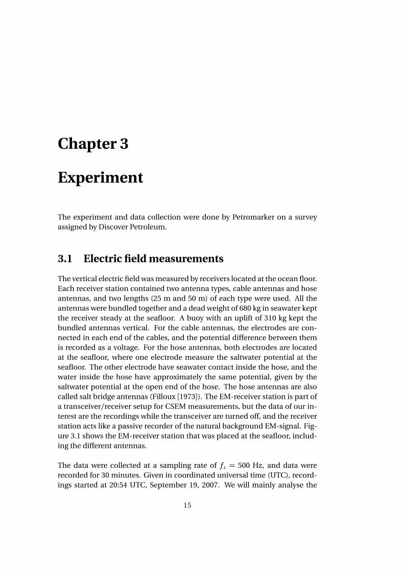
The vertical electric field was measured by receivers located at the ocean floor.Each receiver station contained two antenna types, cable antennas and hoseantennas, and two lengths (25 m and 50 m) of each type were used. All theantennas were bundled together and a dead weight of 680 kg in seawater keptthe receiver steady at the seafloor. A buoy with an uplift of 310 kg kept thebundled antennas vertical. For the cable antennas, the electrodes are con-nected in each end of the cables, and the potential difference between themis recorded as a voltage. For the hose antennas, both electrodes are locatedat the seafloor, where one electrode measure the saltwater potential at theseafloor. The other electrode have seawater contact inside the hose, and thewater inside the hose have approximately the same potential, given by thesaltwater potential at the open end of the hose. The hose antennas are alsocalled salt bridge antennas (Filloux [1973]). The EM-receiver station is part ofa transceiver/receiver setup for CSEM measurements, but the data of our in-terest are the recordings while the transceiver are turned off, and the receiverstation acts like a passive recorder of the natural background EM-signal. Fig-ure 3.1 shows the EM-receiver station that was placed at the seafloor, includ-ing the different antennas.
The data were collected at a sampling rate of f s = 500 Hz, and data wererecorded for 30 minutes. Given in coordinated universal time (UTC), record-ings started at 20:54 UTC, September 19, 2007. We will mainly analyse the
15
16 CHAPTER 3. EXPERIMENT
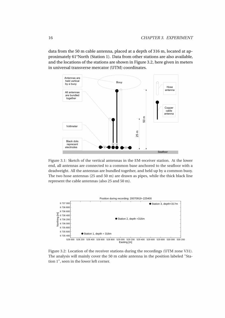
data from the 50 m cable antenna, placed at a depth of 316 m, located at ap-proximately 61°North (Station 1). Data from other stations are also available,and the locations of the stations are shown in Figure 3.2, here given in metersin universal transverse mercator (UTM) coordinates.
Figure 3.1: Sketch of the vertical antennas in the EM-receiver station. At the lowerend, all antennas are connected to a common base anchored to the seafloor with adeadweight. All the antennas are bundled together, and held up by a common buoy.The two hose antennas (25 and 50 m) are drawn as pipes, while the thick black linerepresent the cable antennas (also 25 and 50 m).
528 000 528 200 528 400 528 600 528 800 529 000 529 200 529 400 529 600 529 800 530 000 530 200
6 735 400
6 735 600
6 735 800
6 736 000
6 736 200
6 736 400
6 736 600
6 736 800
6 737 000
Station 1, depth = 316m
Station 3, depth=317m
Station 2, depth =316m
Position during recording: 20070919−225400
Easting [m]
Nor
thin
g [m
]
Figure 3.2: Location of the receiver stations during the recordings (UTM zone V31).The analysis will mainly cover the 50 m cable antenna in the position labeled "Sta-tion 1", seen in the lower left corner.
3.2. MEASUREMENTS OF ANTENNA MOTION 17
3.2 Measurements of antenna motion
As the movement of the EM-receivers and the water around the antenna in-duce unwanted signals, the purpose of measuring the position (and velocity)of the EM-receivers, is to achieve an independent data series that can be usedto remove or predict this unwanted electric field.
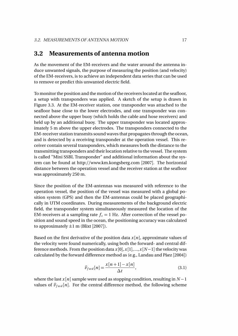
To monitor the position and the motion of the receivers located at the seafloor,a setup with transponders was applied. A sketch of the setup is drawn inFigure 3.3. At the EM-receiver station, one transponder was attached to theseafloor base close to the lower electrodes, and one transponder was con-nected above the upper buoy (which holds the cable and hose receivers) andheld up by an additional buoy. The upper transponder was located approx-imately 5 m above the upper electrodes. The transponders connected to theEM-receiver station transmits sound waves that propagates through the ocean,and is detected by a receiving transponder at the operation vessel. This re-ceiver contain several transponders, which measures both the distance to thetransmitting transponders and their location relative to the vessel. The systemis called "Mini SSBL Transponder" and additional information about the sys-tem can be found at http://www.km.kongsberg.com [2007]. The horizontaldistance between the operation vessel and the receiver station at the seafloorwas approximately 250 m.
Since the position of the EM-antennas was measured with reference to theoperation vessel, the position of the vessel was measured with a global po-sition system (GPS) and then the EM-antennas could be placed geographi-cally in UTM coordinates. During measurements of the background electricfield, the transponder system simultaneously measured the location of theEM-receivers at a sampling rate f s = 1 Hz. After correction of the vessel po-sition and sound speed in the ocean, the positioning accuracy was calculatedto approximately±1 m (Blixt [2007]).
Based on the first derivative of the position data x [n ], approximate values ofthe velocity were found numerically, using both the forward- and central dif-ference methods. From the position data x [0],x [1], ...,x [N−1] the velocity wascalculated by the forward difference method as (e.g., Landau and Pàez [2004])
bv f w d [n ] =x [n +1]−x [n ]
∆t, (3.1)
where the last x [n ] sample were used as stopping condition, resulting in N−1values of bv f w d [n ]. For the central difference method, the following scheme
18 CHAPTER 3. EXPERIMENT
was used (e.g., Landau and Pàez [2004])
bvc e nt [n ] =x [n +1]−x [n −1]
2∆t. (3.2)
Here, the first and the last samples, x [0] and x [N − 1], were used as startingand stopping conditions. Thus, from N samples of x [n ], we get N −2 samplesof the velocity when using the central difference method.
Figure 3.3: Setup of the antennas position measurement. The receiving transponderis attached to the operation vessel, one transmitting transponders is attached to theseafloor base (where the lower electrodes are located), and one to the main buoy, heldup by an additional buoy. The upper transponder is therefore located 5 m above theupper electrodes. The EM-receiver station is shown as the thick black line in the lowerpart of the figure.

Chapter 4
Signal analysis and processingmethods
To examine and characterise the measured data, we will in this chapter presenta number of nonparametric methods. The nonparametric approach is a nat-ural choice when a priori information of statistical properties of the signal isunknown. The presented methods will cover stationarity (runs-test), proba-bility density function (Parzen kernel estimation) and the most thorough partwill cover the power spectrum density (multitaper estimators, and the multi-taper F -test).
19
20 CHAPTER 4. SIGNAL ANALYSIS AND PROCESSING METHODS
4.1 Statistical properties
To characterise the measured data it is useful to estimate the mean and thevariability (by the standard deviation or the variance) of the data. In addition,skewness and kurtosis gives us measures of how the data is distributed rela-tive to normal distributed data.
For a random variable X , the statistical properties can be described by its mo-ments. The arithmetic mean is defined as the first moment about zero (e.g.,Stuart and Ord [1987](§ 2.3)),
µ= E X =∫ ∞
−∞x f (x )d x .
Here, E · denotes the expectation operator, and f (x ) denotes the probabilitydensity function (PDF) of X . The measure of spread around the mean valueis given by the variance σ2, or the standard deviation σ, which is the positivesquare root of the variance and in same units as the mean. The variance isgiven as the second moment about mean (e.g., Stuart and Ord [1987](§ 2.19))
m2 =σ2 = E¦
X −µ2©=
∫ ∞
−∞(x −µ)2 f (x )d x .
If X is a Gaussian distributed random variable, then the PDF is fully describedby the mean and variance.
Skewness is a dimensionless measure of the asymmetry of the PDF (aroundits mean). It is given as the third moment about mean, normalised byσ3 (e.g.,Stuart and Ord [1987](§ 3.31)),
s k =m3
σ3=
E¦
X −µ3©
σ3.
Gaussian distributions are symmetric, and hence have zero skewness. Nega-tive skewness indicate a non Gaussian left skewed PDF with more data in theleft tail (right skewed if skewness is positive).
Kurtosis is a measure for the "peakedness" around the mean (also dimen-sionless), and the weight of the tails compared to a Gaussian PDF. It is givenby the fourth moment about mean, normalised by σ4 (e.g., Stuart and Ord[1987](§ 3.31)),
k =m4
σ4=
E¦
X −µ4©
σ4−3.
4.2. ESTIMATION OF THE PROBABILITY DENSITY 21
Here, the number three is subtracted to give zero kurtosis for the Gaussiandistribution. Compared to a Gaussian distribution, negative kurtosis indicatea PDF which is more flat around mean and with lighter tails. A positive kur-tosis indicates a PDF which is more peaked around mean and with heaviertails.
4.1.1 Sample moments
The following estimators will be used to calculate the sample moments basedon the sampled data x [n ] (e.g., Press et al. [1992](Ch. 14.1)).
Mean: x =1
N
N−1∑
n=0
x [n ], (4.1)
Standard deviation: bσ=s
1
N −1
N−1∑
n=0
(x [n ]−x )2, (4.2)
Variance: bσ2 =1
N −1
N−1∑
n=0
(x [n ]−x )2, (4.3)
Skewness: cs k =1
bσ3N
· 1
N
N−1∑
n=0
(x [n ]−x )3, (4.4)
Kurtosis: bk = 1
bσ4N
· 1
N
N−1∑
n=0
(x [n ]−x )4−3. (4.5)
Note that for the skewness and kurtosis estimators, we will divide by the bi-ased estimator bσN of the standard deviation
bσN =
s1
N
N−1∑
n=0
(x [n ]−x )2.
4.2 Estimation of the probability density
In addition to the sample moments, an estimate of the probability densityfunction (PDF) is useful to reveal the statistical nature of the observed data.For a random variable X , the PDF is defined as f (x )≥ 0, ∀x , and
∫∞−∞ f (x )d x = 1.
From the PDF we can also find the probability of X being within a given inter-val, e.g., the probability of X being between a and b is given by (e.g, Silverman[1986])
P(a ≤X ≤b ) =
∫ b
a
f (x )d x .
22 CHAPTER 4. SIGNAL ANALYSIS AND PROCESSING METHODS
4.2.1 Histogram
The most basic estimator of the PDF is the normalised histogram. Here, theamplitude of the data are distributed in a user selected number of bins. Wecount the number of samples in each bin, and by dividing this number bytotal number of samples and the binwidth, we get a crude estimate of theprobability for a sample falling into the different bins. For the observed datadenoted xn , and n = 1, 2, ..., N , binwidth b and number of samples N , thehistogram estimator of the PDF can be written as (Wand and Jones [1995])
bf (x ) = no. of observations of xn in bin centered at x
N b. (4.6)
This estimator results in a discontinuous function, which is very sensitive toour choice of number and width of the bins.
4.2.2 Parzen window estimator
A more convenient method than the histogram is the Parzen window estima-tor, named after the inventor Parzen [1962]. Here, a smooth and normalisedfunction, a so-called kernel, is centered with its origin at each data point xn .By summing the kernels we achieve a continuous estimate, which also hasgood statistical properties (e.g., Parzen [1962], Wand and Jones [1995] andHanssen et al. [2003]).
If we have N independent identically distributed samples xn , and n = 1, 2, ..., N ,the kernel estimate of the PDF at amplitude x , is given by Parzen [1962],
bf (x ) = 1
N
N∑
n=1
1
bφx −xn
b
. (4.7)
At every x position we place the smoothing kernel φ(·) and by (x − xn ) thekernel will be centered with its origin in each data point xn . The sum of allthe kernel values at amplitude x is then scaled to get the estimated value bf (x ).The binwidth parameter b , is now a width parameter defining the shape ofthe kernel function φ(·) and thereby also gives the level of smoothing. For avalid estimator the kernel function need to fulfil the following constraints
φ(v )≥ 0 and
∫ ∞
−∞φ(v )d v = 1, (4.8)
where v = (x − xn )/b . To ensure that the estimate in Eq. (4.7) results in adensity, the kernel is chosen to be a symmetric distribution function. The
4.3. STATIONARITY 23
standard Gaussian distribution function (N (0, 1))
φ(v ) =
1/p
2π
exp−v 2/2
, (4.9)
is a good standard choice (e.g., Theodoridis and Koutroumbas [1998] and Hanssenet al. [2003]), and will be the smoothing kernel used in this thesis. The choiceof the width parameter b is crucial for our estimate. If b is too small, the vari-ance of the estimate will be unacceptable, and if b is too big, the bias increasesand we lose details in the estimate. Under the assumptions of Gaussian ob-served data and a Gaussian kernel, an optimal value of b is given by (Silver-man [1986])
b = bσ
4
3N
(1/5), (4.10)
where bσ is calculated from the observed data using the sample standard de-viation in Eq. (4.2).
4.3 Stationarity
Several classes of stationarity exist, where a strict stationarity process is onefor which the probability density function of all orders do not change withtime. This is a very strict and difficult task to test for in a given sample ofdata. The spectrum estimation methods in the following sections are devel-oped based on the assumption of wide-sense (or weak) stationary process.For a stochastic process X (t ), the process is called wide-sense stationary if thefollowing conditions are met (e.g., Bendat and Piersol [2000]):
1. E X (t )= constant
2. RX X (t1, t2) = E X (t1)X (t2)= E X (0)X (τ)=RX X (τ).
In words, the expectation value does not change with time, and the autocor-relation between the process X t1 observed at time t1 and X t2 at time t2 onlydepends on the time difference τ = t2 − t1. If only the first condition is met,the process is called stationary in the mean.
In this thesis we will check if the mean and the variance change with timeusing the so-called runs test (e.g., Shiavi [1999]). For the spectrum estimatorsin the following sections, a nonstationary process will cause bias in the esti-mates. For example, if we record data for a given time T , and the data containsa signal with period greater than T , this will cause the mean to change withtime and hence the data set will be nonstationary. In the spectrum estimatethis will cause a bias for the lowest frequencies.
24 CHAPTER 4. SIGNAL ANALYSIS AND PROCESSING METHODS
4.3.1 Runs Test
To test whether the data come in a random order, the nonparametric runstest can be used to check for trends in the sample moments (e.g the mean andvariance). We will here use the method as explained in the book Shiavi [1999](p.198). The data set is divided into Ns subsets, and the sample mean (or othermoments) are calculated for each subset, giving a sequence of Ns mean val-ues. We then find the median value of this sequence (median of the samplemean from all subsets). By comparing the mean values and the median valuewe generate a run sequence that only indicate if the subset value is greater (+)or less (-) than the median value, e.g.,
runs sequence : [+−+++−−+−−−+]
We now count the numbers of runs, r , where adjacent subsequences of samesign is counted as a run, also including single events of a sign as one run. Alter-natively, the number of runs can be counted as numbers of sign changes, in-cluding the first sign as a change of sign (included as 1 in following equation),r = 1+ (number of sign changes). For the runs sequence above, the numberof runs is r = 7.
From Shiavi [1999] the number of runs have a mean and variance given by
mr = (Ns/2)+1 σ2r =
Ns (Ns −2)4(Ns −1)
. (4.11)
The null hypotesis is that the runs sequence is Ns independent measures fromthe same random variable. To form the confidence interval we use the tablein Shiavi [1999](p.199). For example, if Ns = 10, the 95% confidence inter-val is given by 2 < r ≤ 9. An approximately 95% interval can be formed as[mr −2σr ≤ r ≤mr +2σr ], where 2σr is rounded off to the nearest integer. Ifthe number of runs is outside the confidence interval, we reject the randomorder hypothesis, which also indicate nonstationary data.
An alternative method to the runs test could be the reverse arrangement methodgiven in Bendat and Piersol [2000](p.105)
4.4. POWER SPECTRUM ESTIMATION 25
4.4 Power spectrum estimation
4.4.1 Definition of the power spectrum density
When analysing real data, the estimation of the power spectrum density (PSD)is useful to predict the power contribution from different frequency intervals,and hence help us to describe and understand the observed time-series. Wewill now define the power spectral density following Hanssen [2003]. Simi-lar approaches are also given in e.g., Percival and Walden [1993] and Shiavi[1999].
To calculate the energy and the Fourier transform of a realization x (t ) of thestochastic process X (t ), it needs to be absolute integrable (
∫∞−∞ |x (t )|d t <∞).
For a stochastic process that fluctuates/oscillates for infinite time, neither thetotal energy nor the Fourier transform can be calculated. However, if we ob-serve x (t ) in the limited time interval−T < t < T , the truncated variable xT (t )is given as
xT (t ) =
¨x (t ) , −T < t < T
0 , elsewhere.(4.12)
Now, the truncated variable can be Fourier transformed as usual,
XT ( f ) =
∫ ∞
−∞xT (t )e−j 2π f t d t =
∫ T
−T
x (t )e−j 2π f t d t . (4.13)
By Parseval’s theorem the energy of a signal is conserved in both time andfrequency domain. The energy of x (t ) in the given time interval is given as
ε=
∫ T
−T
|x (t )|2d t =
∫ ∞
−∞
XT ( f )2 d f , (4.14)
where XT ( f ) denotes the Fourier transform of xT (t ). Since the energy of astochastic process does not exist, we instead calculate the total average power(energy per time). The truncated xT (t ) is observed during a time interval oflength 2T . If we then let T →∞, and introduce the expectation operator orensemble average E ·, the total average power of x (t ) can be defined as
P = limT→∞
∫ T
−TE|x (t )|2d t
2T=
∫ ∞
−∞lim
T→∞E|XT ( f )|2
2Td f . (4.15)
The integrand,
limT→∞
E|XT ( f )|2
2T, (4.16)
26 CHAPTER 4. SIGNAL ANALYSIS AND PROCESSING METHODS
is obviously a density in the frequency domain, and it is called the power spec-trum density (PSD). By expressing Eq. (4.16) in terms of x (t ) (see Eq. (4.13)),we obtain the fundamental definition of the PSD, denoted S( f ), for a stochas-tic signal
S( f ) = limT→∞
E
1
2T
∫ T
−T
x (t )e−j 2π f t d t
2
. (4.17)
The estimators of the power spectrum density in the following sections will bebased the definition in Eq. (4.17).
4.4.2 Basic power spectrum estimators
We will now look at the basic estimators for the power spectrum density, theperiodogram and the modified periodogram, following Hanssen [2003]. Othergood sources are e.g., Percival and Walden [1993] and Shiavi [1999].
If we have N equally spaced samples x [n ] of x (t ), sampled every ∆t , an es-timator of the power spectrum density, can be derived from the definitionin Eq. (4.17). We have to disregard the expectation operator since we knowthe values of x [n ] only for the finite time 2T , now given by 2T = N∆t . Fur-thermore, we also need to remove the limT→∞ operator. Finally, we convertthe Fourier transform to a Discrete Time Fourier transform (DTFT), given byX ( f ) = ∆t
∑N−1n=0 x [n ]e−j 2π f n∆t . The basic estimator, called the periodogram,
now becomes
bS(p e r )( f ) =1
N∆t
X ( f )2 = ∆t
N
N−1∑
n=0
x [n ]e−j 2π f n∆t
2
; | f | ≤ 1/(2∆t ). (4.18)
Before further discussion we first derive the expectation properties of the pe-riodogram,
E bS(p e r )( f )= ∆t
N·E(
N−1∑
n=0
N−1∑
m=0
x [n ]e−j 2πn∆t x [m ]e j 2πn∆t
). (4.19)
The expectation operator E · works only on the stochastic terms x [n ] andx [m ], giving E x [n ]x [m ]. This is equal to the autocorrelation function RX X [n ,m ].We then assume the data are from a wide sense stationary process, then RX X [n , m ] =Rx x [n−m ] and by the Wiener-Khinchin relation, the following can be replacedin Eq. (4.19)
E x [n ]x [m ]=RX X [n −m ] =
∫ 1/2∆t
−1/2∆t
S( f ′)e j 2π f ′(n−m )∆t d f ′, (4.20)
4.4. POWER SPECTRUM ESTIMATION 27
where S( f )denotes the true spectrum. When inserting Eq. (4.20) into Eq. (4.19)we obtain
E bS(p e r )( f )= ∆t
N
∫ 1/2∆t
−1/2∆t
S( f ′)N−1∑
n=0
e−j 2π( f − f ′)∆tN−1∑
m=0
e j 2πm ( f − f ′)∆t d f ′
=∆t
N
∫ 1/2∆t
−1/2∆t
S( f ′)
N−1∑
n=0
e−j 2π( f − f ′)n∆t
2
d f ′.
(4.21)
If we now gather the parts not containing the true spectrum S( f ), we get thefundamental Dirichlet kernel (Percival and Walden [1993]), here denoted D( f )
D( f ) =∆t
N
N−1∑
n=0
e−j 2π( f )n∆t
2
=∆t
N
N−1∑
n=0
e−j 2πn∆tN−1∑
m=0
e j 2πm∆t =∆t
N
sin2(Nπ f∆t )sin2(π f∆t )
.
(4.22)Returning to Eq. (4.21) we see that the expectation of the periodogram be-comes a convolution between the Dirichlet kernel D( f ) and the true spec-trum,
E bS(p e r )( f )=∫ 1/2∆t
−1/2∆t
D( f − f ′)S( f ′)d f ′ =D( f ) ∗S( f ). (4.23)
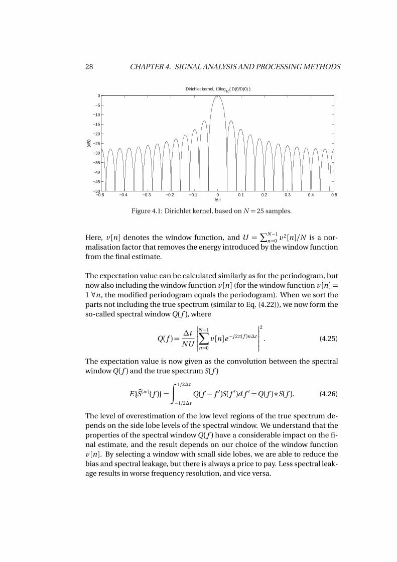
This is an important and fundamental result when discussing spectral esti-mators. The convolution results in a smoothing of the true spectrum andan unwanted smearing of the power. The Dirichlet kernel is shown in Fig-ure 4.1. The main lobe, centred at f = 0 has a width of 2/N∆t and a mainlobe side lobe ratio of 13 dB. The high levels of the side lobes cause spectralleakage, due to the convolution, where the power of the true spectrum leaksvia the side lobes and causes a smoothing of the true spectrum. In general,peaked areas of the true spectrum will be underestimated, and low level re-gions will be overestimated. In particular, the spectral leakage from maximaof the true spectrum cause overestimated levels in frequency intervals werethe true spectrum level is low, and peaks and features in these interval can betotally hidden in the estimate.
By the use of a window function that weights the samples of x [n ] in time do-main, we can modify the Dirichlet kernel spectral properties, to achieve lowerside lobes and better control of the bias of the estimate. This estimator iscalled the modified periodogram or windowed periodogram, and can be writ-ten as
bS(w )( f ) = ∆t
NU
N−1∑
n=0
v [n ]x [n ]e−j 2π f∆t
2
. (4.24)
28 CHAPTER 4. SIGNAL ANALYSIS AND PROCESSING METHODS
−0.5 −0.4 −0.3 −0.2 −0.1 0 0.1 0.2 0.3 0.4 0.5−50
−45
−40
−35
−30
−25
−20
−15
−10
−5
0
f∆ t
(dB
)Dirichlet kernel, 10log
10( D(f)/D(0) )
Figure 4.1: Dirichlet kernel, based on N = 25 samples.
Here, v [n ] denotes the window function, and U =∑N−1
n=0 v 2[n ]/N is a nor-malisation factor that removes the energy introduced by the window functionfrom the final estimate.
The expectation value can be calculated similarly as for the periodogram, butnow also including the window function v [n ] (for the window function v [n ] =1 ∀n , the modified periodogram equals the periodogram). When we sort theparts not including the true spectrum (similar to Eq. (4.22)), we now form theso-called spectral window Q( f ), where
Q( f ) =∆t
NU
N−1∑
n=0
v [n ]e−j 2π( f )n∆t
2
. (4.25)
The expectation value is now given as the convolution between the spectralwindow Q( f ) and the true spectrum S( f )
E bS(w )( f )=∫ 1/2∆t
−1/2∆t
Q( f − f ′)S( f ′)d f ′ =Q( f ) ∗S( f ). (4.26)
The level of overestimation of the low level regions of the true spectrum de-pends on the side lobe levels of the spectral window. We understand that theproperties of the spectral window Q( f ) have a considerable impact on the fi-nal estimate, and the result depends on our choice of the window functionv [n ]. By selecting a window with small side lobes, we are able to reduce thebias and spectral leakage, but there is always a price to pay. Less spectral leak-age results in worse frequency resolution, and vice versa.

4.5. MULTITAPER POWER SPECTRUM ESTIMATION 29
In the asymptotic limit (N →∞), it can be shown (e.g., Percival and Walden[1993](p.222)) that the variance of the periodogram and the modified peri-odogram can be approximated as
var¦bS(w )( f )
©≈S2( f ), (4.27)
for 0< f < f (N ), where f (N ) = 1/(2∆t ) is the Nyquist frequency . To summarise,the periodogram is generally biased, but by the use of a good window func-tion, we are able to reduce the bias. Both the periodogram and windowedperiodogram is inconsistent since the variance do not reduce when we in-crease N . The high variance makes these estimators less trustworthy, and noscientific conclusions should be made based on only one estimate using these"single-window" estimators.
4.5 Multitaper power spectrum estimation
The multitaper (MT), or multi window spectrum estimator is an extensionof the "single-window" periodogram as given in Eq. (4.24). Thomson [1982]proposed to use several orthogonal window functions called discrete prolatespheroidal sequences (DPSS) to form several modified periodograms that canbe applied on the same data. Averaging the modified periodograms, also calledeigenspectra, results in an advantageous reduction of the variance.
4.5.1 Selecting the optimal window functions - discreteprolate spheroidal sequences
The windowed periodogram has been used to reduce the spectral leakage bythe use of window functions (also called tapers) that manipulate the Dirich-let’s kernel, and reduces the level of the sidelobes. The Hamming and Hanningwindows are the most familiar, and they are just two examples out of the manywindows that have been studied. The papers by Harris [1978], Nuttall [1981]and Kaiser and Schafer [1980] contain extensive research on the conventionalwindow functions and their spectral properties.
Instead of studying the spectral properties of various more than less inciden-tal windows to find the optimal window function, Slepian [1978] presented adifferent approach (for review see Slepian [1983]). He started out with somecriteria which ensure that the window functions with the best leakage proper-ties for a given frequency resolution can be derived. This is commonly calledthe concentration problem (e.g., Percival and Walden [1993]). The solution of
30 CHAPTER 4. SIGNAL ANALYSIS AND PROCESSING METHODS
the problem is an eigenvalue equation, were the DPSS are the eigenvectorsof the equation. The zeroth order DPSS is the window function that providethe best leakage properties (e.g., Eberhard [1973]). In the innovative paper byThomson [1982], the properties of the DPSS were a central part of the deriva-tion of the multitaper method, and Thomson proposed to use several of theDPSS obtained from the eigenvalue equation in spectrum estimation.
The eigenvalue equation defining the DPSS can be derived as follows:
1. The spectral concentration λ in the mainlobe should be maximised.For a user specified resolution bandwidth 2W (given in normalised fre-
quency), the power in the mainlobe is given by∫W
−WQ( f )d f , and the
total power of the spectral window is∫ 1/2
−1/2Q( f )d f . The spectral con-
centration can now be defined as the ratio between the energy in themainlobe and the total energy,
λ=
∫W
−WQ( f )d f
∫ 1/2
−1/2Q( f )d f
. (4.28)
For an ideal choice of Q( f ), all the window energy will be located in themainlobe and λ= 1.
2. The spectral window should be normalised∑N−1
n=0 v 2[n ] = 1. If we rep-resent v [n ] as a vector v = [v0,v1, ...vN−1]T , this can be expressed asvT v= 1.
For simplicity we choose∆t = 1 in this section. Since the v [n ] is normalised,the scaling outside the absolute sign in Eq. (4.25), reduces to
U = 1/NN−1∑
n=0
v 2[n ] = 1/N ,
and ∆t /NU = 1. The purpose is now to find the window function v [n ] thatmaximises λ. We start by writing out Eq. (4.28) using definition Eq. (4.25).First, we consider the numerator
∫ W
−W
Q( f )d f =
∫ W
−W
N−1∑
n=0
v [n ]e−j 2π f nN−1∑
m=0
v [m ]e j 2π f m d f
=N−1∑
n=0
v [n ]
∫ W
−W
e−j 2π f (n−m )df
!N−1∑
m=0
v [m ]
=N−1∑
n=0
v [n ]
sin(2πW [n −m ])π[n −m ]
N−1∑
m=0
v [m ].
(4.29)
4.5. MULTITAPER POWER SPECTRUM ESTIMATION 31
If we now use vector/matrix notation and define the matrix A as[A]nm = sin(2πW [n −m ])/π[n −m ], the numerator can be written as
∫ W
−W
Q( f )d f = vT A v.
For the denominator, we derive the following expression,
∫ 1/2
−1/2
Q( f )d f =N−1∑
n=0
v [n ]
∫ 1/2
−1/2
e−j 2π f (n−m )df
!N−1∑
m=0
v [m ]
=N−1∑
n=0
v [n ]
sin[π(n −m )]π(n −m )
N−1∑
m=0
v [m ]
=
N−1∑
n=0
v [n ]N−1∑
m=0
v [m ]
!δ[n −m ]
=N−1∑
n=0
w 2[n ] = vT v.
(4.30)
Furthermore, we can now write Eq. (4.28) as
λ=vT A v
vT v. (4.31)
To find the sequence v that maximises λ, we need to differentiate λ with re-spect to v in the latter equation, to obtain the criterion
∂ λ
∂ v= 0 =⇒ 2A v(vT v)− (vT A v)2v
(vT A v)2= 0. (4.32)
If we now insert (vT A v) =λ(vT v) from Eq. (4.31), we obtain
2A v(vT v)−λ(vT v)2v
(vT v)2= 0. (4.33)
The above equation is true as long as the numerator is equal to the zero vector,and we then end up with the fundamental eigenvalue equation from whichthe window function v [n ]with the best leakage properties can be derived,
A v=λv. (4.34)
For a matrix A of size N ×N the eigenvalue equation will have N eigenval-ues with corresponding N × 1 eigenvectors, (λ0, v0), (λ1, v1), ..(λN−1, vN−1). The
32 CHAPTER 4. SIGNAL ANALYSIS AND PROCESSING METHODS
eigenvaluesλk simply represent the spectral concentration for the correspond-ing eigenvector vk , and will always be between 1 and 0 in the order,
1≥λ0 ≥λ1 ≥ ...≥λN−1 ≥ 0.
Since λ0 is the largest eigenvalue, the corresponding eigenvector v0 has thegreatest spectral concentration of all the eigenvectors, and hence the optimalleakage properties. The eigenvectors are orthogonal to each other, vT
k vl =δ[k − l ],and named discrete prolate spheroidal sequences (DPSS), or Slepian sequencesafter the inventor.
For spectrum estimation, the DPSS provides a selection of orthogonal win-dows with optimal leakage properties, and the multitaper method was formedbased on these windows (Thomson [1982]). To find the DPSS for a givenlength N and frequency resolution 2W , Eq. (4.34) will have to be solved nu-merically. In Matlab, the function ’dpss’ can be used, while Lees and Park[1995] provide C-subroutines for the purpose.
In Figure 4.2 the Dirichlet kernel, Hanning, Hamming and Kaiser windowfunctions are plotted together with the zeroth-order DPSS (k = 0), and theirrespective normalised spectral windows |V ( f )/V (0)|2, where V ( f ) denotes theDTFT of v [n ]. For n = 0,1, . . . ,N −1, the window functions are given by
Dirichlet kernel: v [n ] = 1, (4.35)
and (Nuttall [1981])
Hanning: v [n ] = 0.5
1− cos
2πn
N −1
, (4.36)
Hamming: v [n ] = 0.54−0.46cos
2πn
N −1
, (4.37)
and (Kaiser and Schafer [1980])
Kaiser: v [n ] =I0
α
q1−
2·n−(N−1)N−1
2
I0(α). (4.38)
Here,α is a design parameter which changes the shape of the window and I0 isthe modified Bessel function of first kind and zeroth-order, from Harris [1978],
I0(x ) =∑∞
k=0
hx k
2k k !
i2. For the four latter windows the frequency resolution and
the mainlobe width, denoted f M , can be defined as twice the distance fromV ( f = 0) to the first zero-crossing. This implies the following mainlobe width
Dirichlet kernel : f M =2
N∆t,
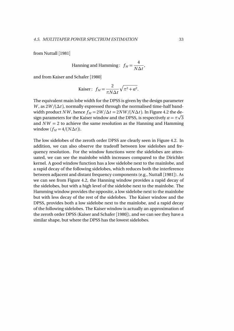
4.5. MULTITAPER POWER SPECTRUM ESTIMATION 33
from Nuttall [1981]
Hanning and Hamming : f M =4
N∆t,
and from Kaiser and Schafer [1980]
Kaiser : f M =2
πN∆t
pπ2+α2.
The equivalent main lobe width for the DPSS is given by the design parameterW , as 2W /(∆t ), normally expressed through the normalised time-half band-width product N W , hence f M = 2W /∆t = 2N W /(N∆t ). In Figure 4.2 the de-sign parameters for the Kaiser window and the DPSS, is respectively α= π
p3
and N W = 2 to achieve the same resolution as the Hanning and Hammingwindow ( f M = 4/(N∆t )).
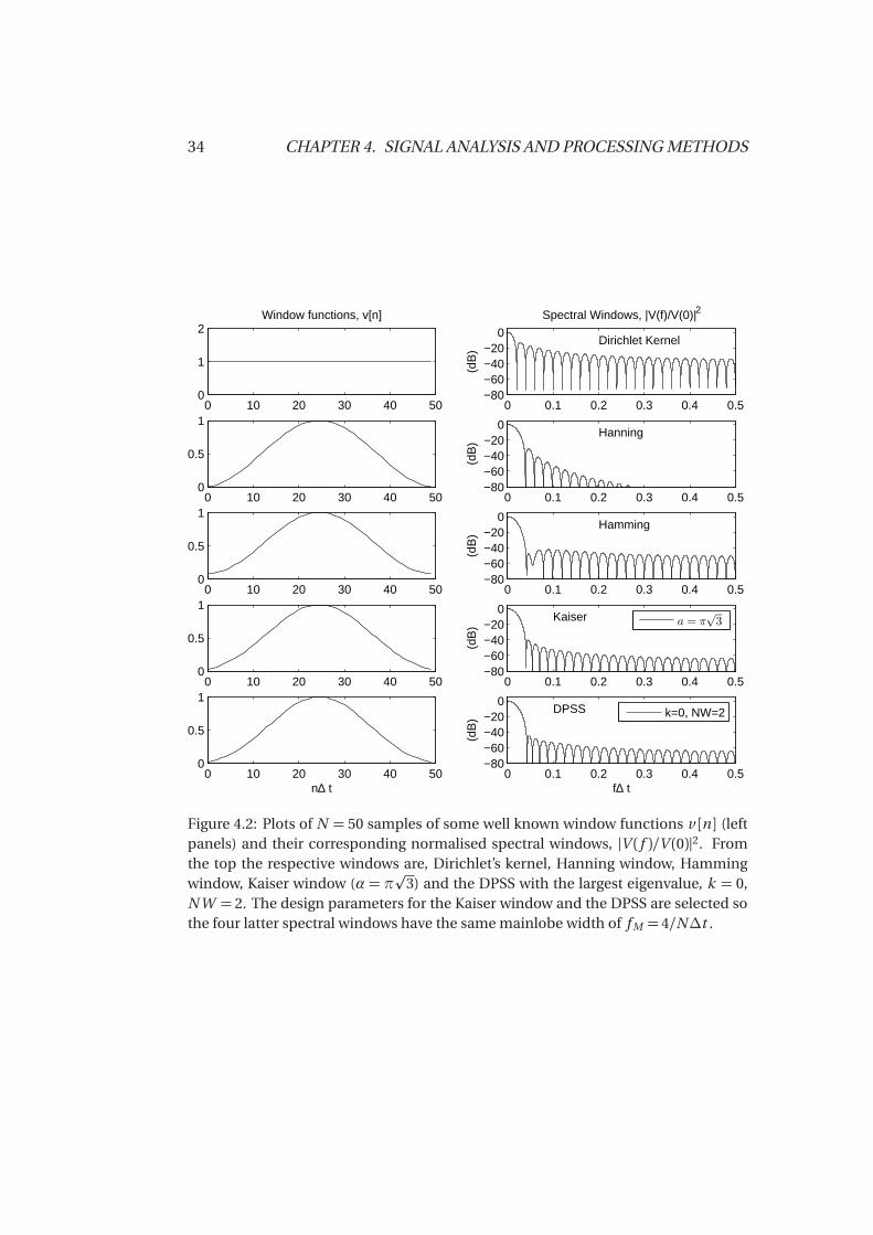
The low sidelobes of the zeroth order DPSS are clearly seen in Figure 4.2. Inaddition, we can also observe the tradeoff between low sidelobes and fre-quency resolution. For the window functions were the sidelobes are atten-uated, we can see the mainlobe width increases compared to the Dirichletkernel. A good window function has a low sidelobe next to the mainlobe, anda rapid decay of the following sidelobes, which reduces both the interferencebetween adjacent and distant frequency components (e.g., Nuttall [1981]). Aswe can see from Figure 4.2, the Hanning window provides a rapid decay ofthe sidelobes, but with a high level of the sidelobe next to the mainlobe. TheHamming window provides the opposite, a low sidelobe next to the mainlobebut with less decay of the rest of the sidelobes. The Kaiser window and theDPSS, provides both a low sidelobe next to the mainlobe, and a rapid decayof the following sidelobes. The Kaiser window is actually an approximation ofthe zeroth order DPSS (Kaiser and Schafer [1980]), and we can see they have asimilar shape, but where the DPSS has the lowest sidelobes.
34 CHAPTER 4. SIGNAL ANALYSIS AND PROCESSING METHODS
0 0.1 0.2 0.3 0.4 0.5−80−60−40−20
0
(dB
)
Spectral Windows, |V(f)/V(0)|2
Dirichlet Kernel
0 0.1 0.2 0.3 0.4 0.5−80−60−40−20
0
(dB
)
Hanning
0 0.1 0.2 0.3 0.4 0.5−80−60−40−20
0
(dB
)
Hamming
0 0.1 0.2 0.3 0.4 0.5−80−60−40−20
0
(dB
)
Kaiser
a = π
√
3
0 0.1 0.2 0.3 0.4 0.5−80−60−40−20
0
(dB
)
DPSS
f∆ t
k=0, NW=2
0 10 20 30 40 500
1
2Window functions, v[n]
0 10 20 30 40 500
0.5
1
0 10 20 30 40 500
0.5
1
0 10 20 30 40 500
0.5
1
0 10 20 30 40 500
0.5
1
n∆ t
Figure 4.2: Plots of N = 50 samples of some well known window functions v [n ] (leftpanels) and their corresponding normalised spectral windows, |V ( f )/V (0)|2. Fromthe top the respective windows are, Dirichlet’s kernel, Hanning window, Hammingwindow, Kaiser window (α = π
p3) and the DPSS with the largest eigenvalue, k = 0,
N W = 2. The design parameters for the Kaiser window and the DPSS are selected sothe four latter spectral windows have the same mainlobe width of f M = 4/N∆t .
4.5. MULTITAPER POWER SPECTRUM ESTIMATION 35
4.5.2 The multitaper estimator
When solving Eq. (4.34), we are only interested in the DPSS (eigenvectors)with low spectral leakage. We therefore only select the eigenvectors with cor-responding eigenvalue λk close to 1. It can be shown that the first eigenvaluesare close to one, while the eigenvalues drop to almost 0 beyond the eigenvaluenumber 2N W . To be sure to only use eigenvectors with low spectral leakageselecting the first K = 2N W − 2 DPSS, is usually safe (Percival and Walden[1993]). Thomson [1982] proposed to use the K first eigenvectors (DPSS) aswindow functions and calculate one modified periodogram for each of them,from now on called the eigenspectrum. The simplest multitaper (MT) estima-tor is the arithmetic average of all these eigenspectra (Thomson [1982])
bS(M T )( f ) =1
K
K−1∑
k=0
bS(M T )k ( f ; k ). (4.39)
The eigenspectrum of order k is denoted by bS(M T )k ( f ;k ), and is given by
bS(M T )k ( f ; k ) =∆t
N−1∑
n=0
vk [n ]x [n ]e−j 2π f n∆t
2
, (4.40)
were the window function vk is the k ’th order DPSS. It should be noted thatthe first eigenspectrum, bS(M T )
k ( f ;0), is the estimate with the best leakage prop-erties of all "single window" estimators with frequency resolution 2W (Eber-hard [1973] and Thomson [1982]). As for the modified periodogram, the ex-pectation value of the eigenspectrum results in a convolution between thespectral window and the true spectrum (Percival and Walden [1993](p.334))
E¦bS(M T )
k ( f )©=Qk ( f ) ∗S( f ), (4.41)
where Qk ( f ) denotes the spectral window for the k ’th DPSS, given by
Qk ( f ) =∆t
N−1∑
n=0
vk [n ]e−j 2π f n∆t
2
.
When we average the K eigenspectra, the expectation value for the multitaperestimate is given by
E¦bS(M T )( f )
©=Q( f ) ∗S( f ), (4.42)
were Q( f ) denotes the average spectral window given by
Q( f ) =1
K
K−1∑
k=0
Qk ( f ). (4.43)
36 CHAPTER 4. SIGNAL ANALYSIS AND PROCESSING METHODS
If x [n ] is sampled from a Gaussian zero mean process, the eigenspectra areapproximately uncorrelated (as long as we select K ≤ 2N W ). This impliesthat the asymptotic variance (N →∞) can be approximated as (Percival andWalden [1993](p.351))
var¦bS(M T )( f )
©≈ 1
K 2
K−1∑
k=0
var¦bS(M T )
k ( f ; k )©≈ S2( f )
K. (4.44)
From Eq. (4.42) and (4.44) we understand that the multitaper method pro-vides control of both the bias and of the variance reduction. By the use of theDPSS and a careful selection of K , we achieve a spectral window Q( f ) withlow side lobes and minimum amount of spectral leakage, and by averagingthe eigenspectra we reduce the variance with a factor 1/K compared to theperiodogram. For a fixed W , the number of K useable eigenspectra increasewith N . Hence, the variance is reduced when we increases N , and the MT es-timator is consistent (Thomson [1982]).
Another well known method used to reduce the variance is the weighted over-lapped segment averaging (WOSA) (Welch [1967]). Here, single-window peri-odograms are applied to overlapping data segments, which are then averaged,hence the variance is reduced. Bronez [1992] compared WOSA and MT interms of resolution bandwidth, leakage and variance. By holding two of themeasures equal in both methods, he showed that the MT always performedbetter than WOSA on the last measure.
In this thesis we will consistently use the averaged multitaper method de-scribed above, and the DPSS window functions. It should be noted that the av-eraged MT can be further extended by adaptive weighting procedures (Thom-son [1982] and e.g, Percival and Walden [1993](Ch.7.4)). In addition, the or-thogonal sinusoidal window functions proposed by Riedel and Sidorenko [1995],can also be used as an alternative to the DPSS in multitaper estimation. Thesinusoidal windows perform similar to the DPSS in many situations, and areless complicated to calculate.
Multitaper estimation example
As an example of the use of the multitaper estimator, we will now use datagenerated by an autoregressive model of order four (AR(4)), and compare thetrue spectrum of the AR(4) model, with the estimated results. The AR(4) modelis given by
x [n ] = 2.7607x [n−1]−3.8106x [n−2]+2.6535x [n−3]−0.9238x [n−4]+ε[n ],
4.5. MULTITAPER POWER SPECTRUM ESTIMATION 37
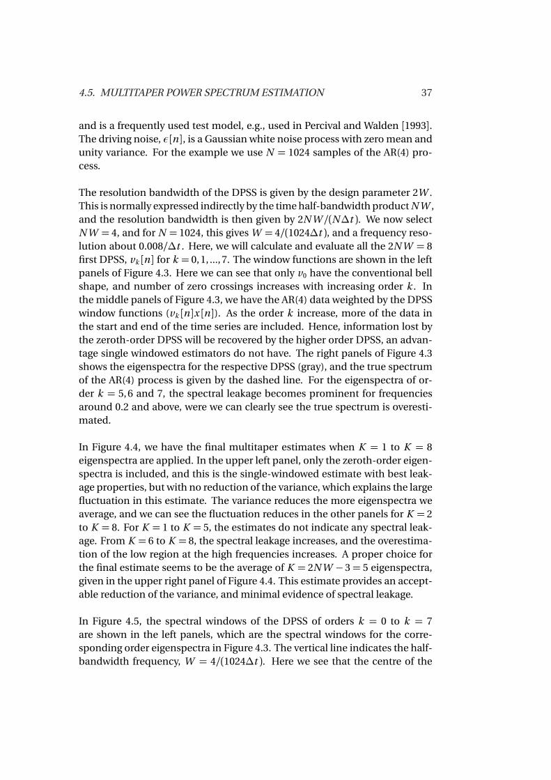
and is a frequently used test model, e.g., used in Percival and Walden [1993].The driving noise, ε[n ], is a Gaussian white noise process with zero mean andunity variance. For the example we use N = 1024 samples of the AR(4) pro-cess.
The resolution bandwidth of the DPSS is given by the design parameter 2W .This is normally expressed indirectly by the time half-bandwidth product N W ,and the resolution bandwidth is then given by 2N W /(N∆t ). We now selectN W = 4, and for N = 1024, this gives W = 4/(1024∆t ), and a frequency reso-lution about 0.008/∆t . Here, we will calculate and evaluate all the 2N W = 8first DPSS, vk [n ] for k = 0, 1, ..., 7. The window functions are shown in the leftpanels of Figure 4.3. Here we can see that only v0 have the conventional bellshape, and number of zero crossings increases with increasing order k . Inthe middle panels of Figure 4.3, we have the AR(4) data weighted by the DPSSwindow functions (vk [n ]x [n ]). As the order k increase, more of the data inthe start and end of the time series are included. Hence, information lost bythe zeroth-order DPSS will be recovered by the higher order DPSS, an advan-tage single windowed estimators do not have. The right panels of Figure 4.3shows the eigenspectra for the respective DPSS (gray), and the true spectrumof the AR(4) process is given by the dashed line. For the eigenspectra of or-der k = 5, 6 and 7, the spectral leakage becomes prominent for frequenciesaround 0.2 and above, were we can clearly see the true spectrum is overesti-mated.
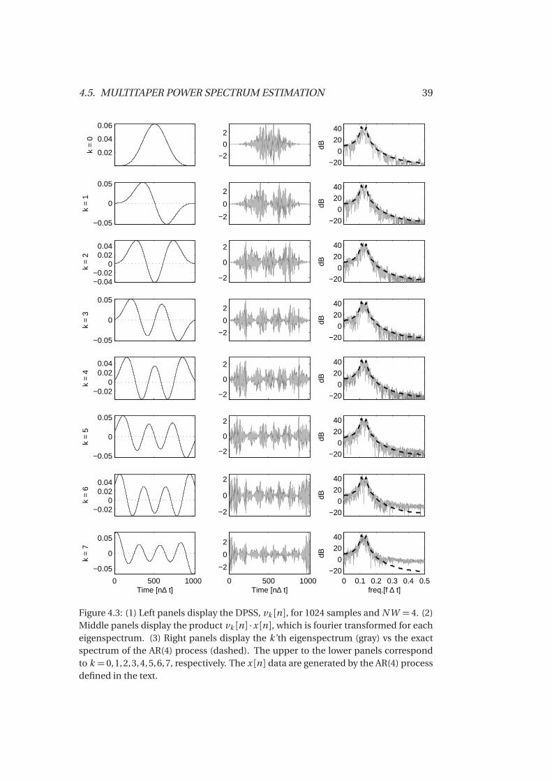
In Figure 4.4, we have the final multitaper estimates when K = 1 to K = 8eigenspectra are applied. In the upper left panel, only the zeroth-order eigen-spectra is included, and this is the single-windowed estimate with best leak-age properties, but with no reduction of the variance, which explains the largefluctuation in this estimate. The variance reduces the more eigenspectra weaverage, and we can see the fluctuation reduces in the other panels for K = 2to K = 8. For K = 1 to K = 5, the estimates do not indicate any spectral leak-age. From K = 6 to K = 8, the spectral leakage increases, and the overestima-tion of the low region at the high frequencies increases. A proper choice forthe final estimate seems to be the average of K = 2N W − 3 = 5 eigenspectra,given in the upper right panel of Figure 4.4. This estimate provides an accept-able reduction of the variance, and minimal evidence of spectral leakage.
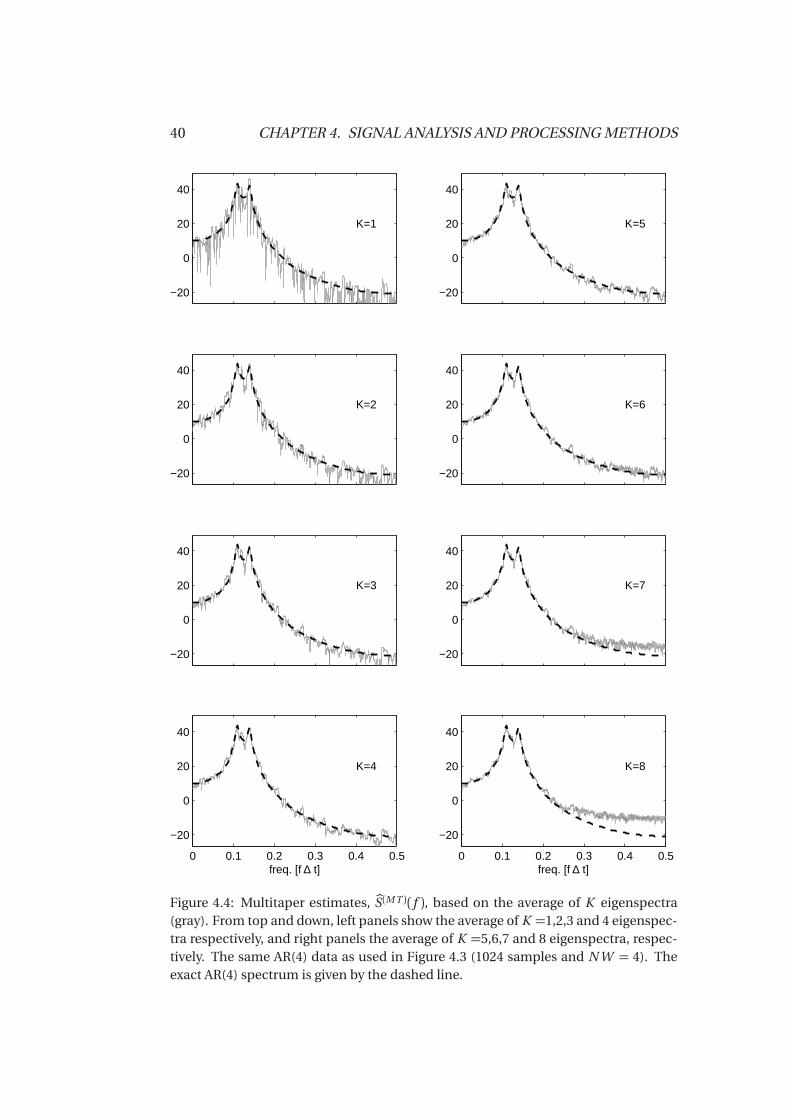
In Figure 4.5, the spectral windows of the DPSS of orders k = 0 to k = 7are shown in the left panels, which are the spectral windows for the corre-sponding order eigenspectra in Figure 4.3. The vertical line indicates the half-bandwidth frequency, W = 4/(1024∆t ). Here we see that the centre of the

38 CHAPTER 4. SIGNAL ANALYSIS AND PROCESSING METHODS
main lobe moves to higher frequencies, and that the levels of the side lobesincrease with increasing order k . We also note that Qk ( f = 0) = 0 for odd k .In the right panels of Figure 4.5 we have the spectral windows Q( f ), corre-sponding to the average multitaper estimates in Figure 4.4. As we increase thenumber of averaged Qk ( f ), the level of the main lobe in Q( f ) become closerto constant, and side lobe levels becomes higher.
To summarise, the best compromise between bias and variance properties forour example seems to be the multitaper estimate based on K = 5 eigenspec-tra (K = 2N W − 3). The final result for this choice is given in the upper rightpanel of Figure 4.4, and the corresponding spectral window Q( f ) is shown inFigure 4.5, from the top, the fifth of the right panels.
4.5. MULTITAPER POWER SPECTRUM ESTIMATION 39
0.02
0.04
0.06
k =
0
−2
0
2
−20
0
20
40
dB
−0.05
0
0.05
k =
1
−2
0
2
−20
0
20
40
dB
−0.04−0.02
00.020.04
k =
2
−2
0
2
−20
0
20
40
dB
−0.05
0
0.05
k =
3
−2
0
2
−20
0
20
40
dB
−0.020
0.020.04
k =
4
−2
0
2
−20
0
20
40
dB
−0.05
0
0.05
k =
5
−2
0
2
−20
0
20
40
dB
−0.020
0.020.04
k =
6
−2
0
2
−20
0
20
40
dB
0 500 1000
−0.05
0
0.05
k =
7
Time [n∆ t]0 500 1000
−2
0
2
Time [n∆ t]0 0.1 0.2 0.3 0.4 0.5
−20
0
20
40
dB
freq.[f ∆ t]
Figure 4.3: (1) Left panels display the DPSS, vk [n ], for 1024 samples and N W = 4. (2)Middle panels display the product vk [n ] ·x [n ], which is fourier transformed for eacheigenspectrum. (3) Right panels display the k ’th eigenspectrum (gray) vs the exactspectrum of the AR(4) process (dashed). The upper to the lower panels correspondto k = 0, 1, 2, 3, 4, 5, 6, 7, respectively. The x [n ] data are generated by the AR(4) processdefined in the text.
40 CHAPTER 4. SIGNAL ANALYSIS AND PROCESSING METHODS
−20
0
20
40
K=1
−20
0
20
40
K=2
−20
0
20
40
K=3
0 0.1 0.2 0.3 0.4 0.5
−20
0
20
40
freq. [f ∆ t]
K=4
−20
0
20
40
K=5
−20
0
20
40
K=6
−20
0
20
40
K=7
0 0.1 0.2 0.3 0.4 0.5
−20
0
20
40
freq. [f ∆ t]
K=8
Figure 4.4: Multitaper estimates, bS(M T )( f ), based on the average of K eigenspectra(gray). From top and down, left panels show the average of K =1,2,3 and 4 eigenspec-tra respectively, and right panels the average of K =5,6,7 and 8 eigenspectra, respec-tively. The same AR(4) data as used in Figure 4.3 (1024 samples and N W = 4). Theexact AR(4) spectrum is given by the dashed line.
4.5. MULTITAPER POWER SPECTRUM ESTIMATION 41
−80−60−40−20
020 k = 0
Qk(f)
dB
−80−60−40−20
020 k = 1
dB
−80−60−40−20
020 k = 2
dB
−80−60−40−20
020 k = 3
dB
−80−60−40−20
020 k = 4
dB
−80−60−40−20
020 k = 5
dB
−80−60−40−20
020 k = 6
dB
0 0.005 0.01 0.015 0.02−80−60−40−20
020 k = 7
freq. [f∆ t]
dB
−80−60−40−20
020 K = 1
Q(f)
dB
−80−60−40−20
020 K = 2
dB
−80−60−40−20
020 K = 3
dB
−80−60−40−20
020 K = 4
dB
−80−60−40−20
020 K = 5
dB
−80−60−40−20
020 K = 6
dB
−80−60−40−20
020 K = 7
dB
0 0.005 0.01 0.015 0.02−80−60−40−20
020 K = 8
freq. [f∆ t]
dB
Figure 4.5: In the left panels, we show the spectral windows, Qk ( f ), for the k ’th orderDPSS, from the top, k = 0, 1, 2, 3, 4, 5, 6, 7 respectively (1024 samples and N W = 4).These are the spectral windows for the respective eigenspectra in Figure 4.3. Thespectral windows for the average multitaper estimates in Figure 4.4, are shown in theright panels and denoted Q( f ). From top and down K = 1, 2, 3, 4, 5, 6, 7, 8 respectively.The vertical line indicate the half-bandwidth W .
42 CHAPTER 4. SIGNAL ANALYSIS AND PROCESSING METHODS
4.6 The chi-square and F -distributions
The chi-square distribution is important for computing confidence intervalsfor the spectrum estimators, while the F distribution will be used in a test tosearch for significant single sinusoidal frequencies in the spectrum. We willfirst define the distributions, and then use them in the following sections.
4.6.1 The chi-square distribution
If we have Y1, Y2, ..., Yν independent Gaussian random variables with zero meanand unity variance, then the sum of the square of the latter variables has a chi-square distribution, χ2
ν , with ν degrees of freedom (e.g., Percival and Walden[1993]
χ2ν = Y 2
1 +Y 22 + ...+Y 2
ν
The chi-square probability density function (PDF) is given by (e.g., Stark andWoods [2002])
f X (x ) =
x (ν−2)/2e−ν/2
2ν/2Γ(ν/2)for x > 0,
0 for x ≤ 0,(4.45)
where the Gamma function Γ(·) is defined as
Γ(β ) =
∫ ∞
0
x (β−1)e−x dx for β > 0. (4.46)
For β equal to a positive integer, i.e., when ν = 2K in Eq. (4.45), the Gammafunction reduces to (β −1)!. The percentage point Qν (p ) is found numerically(Matlab function ’chi2inv’), and related to the chi-square PDF, Eq. (4.45), as
p =
∫ Qν (p )
0
f X (x )dx.
In Figure 4.6, the chi-square distribution is shown for different degrees of free-dom. We can see that when the degrees of freedom increase, the distributionapproach a more symmetric bell shape. The gray part of the curves start at thepercentage point Qν (0.025), and end at the percentage point Qν (0.975), henceindicating the 95% confidence interval.

4.6. THE CHI-SQUARE AND F -DISTRIBUTIONS 43
0 5 10 15 20 250
0.05
0.1
0.15
0.2
0.25
0.3
0.35
0.4
0.45
0.5
x
f X (
x)
Chi−square distribution for selected degrees of freedom (ν)
ν=2ν=5ν=8ν=11
Figure 4.6: Plot of the chi-square distribution for a selection of degrees of freedom.The gray part of the curves start at the 2.5% percentage point Qν (0.025), and end atthe upper 97.5% percentage point Qν (0.975). The area under the gray part representthe 95% of the total area under the curves.
44 CHAPTER 4. SIGNAL ANALYSIS AND PROCESSING METHODS
4.6.2 The F -distribution
As described in Section 4.6.1, the sum of ν squared independent Gaussianvariables with zero-mean and unity variance will have a χ2
ν distribution. TheF -test is defined as the ratio of two χ2
ν variables, each divided by their degreeof freedom (e.g., Bendat and Piersol [2000])
Fν1,ν2 =χ2ν1/ν1
χ2ν2/ν2
, (4.47)
where the ratio Fν1,ν2 is F -distributed and described by the degrees of freedomin both theχ2
ν variables. This test can, e.g., be used to compare the variance oftwo data sets. The probability density function of the F -distribution is givenby (e.g., Bendat and Piersol [2000])
f X (x ) =
Γ[(ν1+ν2)/2]Γ[ν1/2]Γ[ν2/2]
(ν1/ν2)ν1/2 x (ν1/2)−1
[1+(xν1/ν2)](ν1+ν2)/2for x > 0,
0 for x ≤ 0,
(4.48)
where Γ(·) is the Gamma function defined in Eq. (4.46). The percentage pointQν1,ν2(p ) for the 100p % confidence limit is related to Eq. (4.48) as follows
p =
∫ Qν1,ν2 (p )
0
f X (x )dx, (4.49)
and can be found numerically with Matlab command ’finv’. For Thomson’sF -test in Section 4.9, the test is one sided, meaning we are only interestedin the upper percentage point where the calculated Fν1,ν2 value is greater thanQν1,ν2(p ). For this test the degrees of freedom in the numerator will also alwaysbe ν1 = 2 which in turn simplify the calculation of the upper 100p % percent-age point to (e.g., Percival and Walden [1993])
Q2,ν2(p ) =ν2[1− (1−p )2/ν2]
2(1−p )2/ν2. (4.50)
Figure 4.7 displays the F -distribution for several ν2 values (degrees of free-dom in the denominator). The degrees of freedom in the numerator is fixed toν1 = 2, since this will be the case in the F -test in Section 4.9. To better separatethe lines, the function values are given on a logarithmic scale. From the upperpercentage points, Q2,ν2(p ), we can clearly see that when ν2 increases the up-per percentage point decreases, and the function approaches its asymptoticlimit faster.
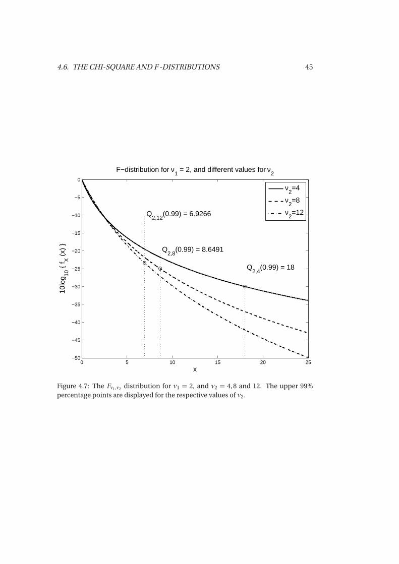
4.6. THE CHI-SQUARE AND F -DISTRIBUTIONS 45
0 5 10 15 20 25−50
−45
−40
−35
−30
−25
−20
−15
−10
−5
0
x
10lo
g 10
f X (
x)
F−distribution for ν1 = 2, and different values for ν
2
Q2,4
(0.99) = 18
Q2,8
(0.99) = 8.6491
Q2,12
(0.99) = 6.9266
ν2=4
ν2=8
ν2=12
Figure 4.7: The Fν1,ν2 distribution for ν1 = 2, and ν2 = 4, 8 and 12. The upper 99%percentage points are displayed for the respective values of ν2.
46 CHAPTER 4. SIGNAL ANALYSIS AND PROCESSING METHODS
4.7 Distribution of spectrum estimates
We will now follow the approach from Percival and Walden [1993] (p.220), andderive the probability distribution of the periodogram. To calculate the con-fidence intervals for the estimator, we need to know the distribution of theestimator. First we rewrite Eq. (4.18) to include the scaling inside the absolutesign,
bS(p e r )( f ) = |J ( f )|2,
where J ( f ) is given by
J ( f ) =∆t
N
1/2 N−1∑
n=0
Gx [n ]e−j 2π f n∆t . (4.51)
The observed data are now denoted Gx [n ] and assumed to be drawn from aGaussian white process, with zero mean and varGx [n ] = σ2. We then eval-uate the real and imaginary parts A( f ) and B ( f ), J ( f ) = A( f )− j B ( f ), givenby
A( f ) =∆t
N
1/2 N−1∑
n=0
Gx [n ]cos
2π f n∆t
,
B ( f ) =∆t
N
1/2 N−1∑
n=0
Gx [n ]sin
2π f n∆t
.
(4.52)
Since Gx [n ] is a Gaussian white process, also A( f ) and B ( f ) will have zeromean,
E
A( f )=∆t
N
1/2 N−1∑
n=0
E Gx [n ]cos
2π f n∆t= E
B ( f )
= 0. (4.53)
The variance is given by
var
A( f )= E
¦A2( f )
©=∆t
N
N−1∑
n=0
E G 2x [n ] cos2(2π f n∆t ),
=σ2∆t
N
N−1∑
n=0
cos2(2π f n∆t )
varB ( f )= ∆t
N
N−1∑
n=0
E G 2x [n ] sin(2π f n∆t )
=σ2∆t
N
N−1∑
n=0
sin2(2π f n∆t ).
(4.54)
4.7. DISTRIBUTION OF SPECTRUM ESTIMATES 47
If we now only evaluate the above equations for the standard frequencies,f m =m/N∆t , where m is an integer, and excluding f m = 0 and the Nyquistfrequency f (N ) = 1/(2∆t )we get
varA( f m )=σ2∆t
2
varB ( f m )=σ2∆t
2.
(4.55)
for 0< f m < f (N ) and m = 1,2, .., N −2. Since A( f m ) and B ( f m ) are orthogonal,they are also uncorrelated, and uncorrelated Gaussian random variables arealso independent. The periodogram is given by
A2( f m )+ B 2( f m ) = bS(p e r )( f m ).
If we scale A( f m ) and B ( f m )with (2/σ2∆t )1/2 the scaled periodogram is then asum of two squared independent random variables with zero mean and unitvariance, and hence, chi-square distributed, with 2 degrees of freedom,
(2
σ2∆t)bS(p e r )( f m )
d=χ22 => bS(p e r )( f m )
d=σ2∆t
2χ2
2 , (4.56)
whered=, denotes equality in distribution. The spectrum for a sampled white
Gaussian process is S( f ) = σ2∆t and hence we can replace the scaling inEq. (4.56) with the true spectrum
bS(p e r )( f m )d=
S( f )2χ2
2 . (4.57)
If the observed data are stationary (not necessary white noise or Gaussiandistributed) and the true spectrum is continuous on the interval [− f (N ), f (N )],each eigenspectrum bS(M T )
k ( f ) is asymptotically distributed as
bS(M T )k ( f ) d=
S( f )2χ2
2 , 0< f < f (N ). (4.58)
The average multitaper estimate is an average of K approximately uncorre-lated eigenspectra, each with ν = 2 degrees of freedom, and hence has 2Kdegrees of freedom. In the asymptotically limit this estimate is distributed asa scaled chi-square distribution with 2K degrees of freedom,
bS(M T )( f ) d=S( f )2K
χ22K , 0< f < f (N ). (4.59)
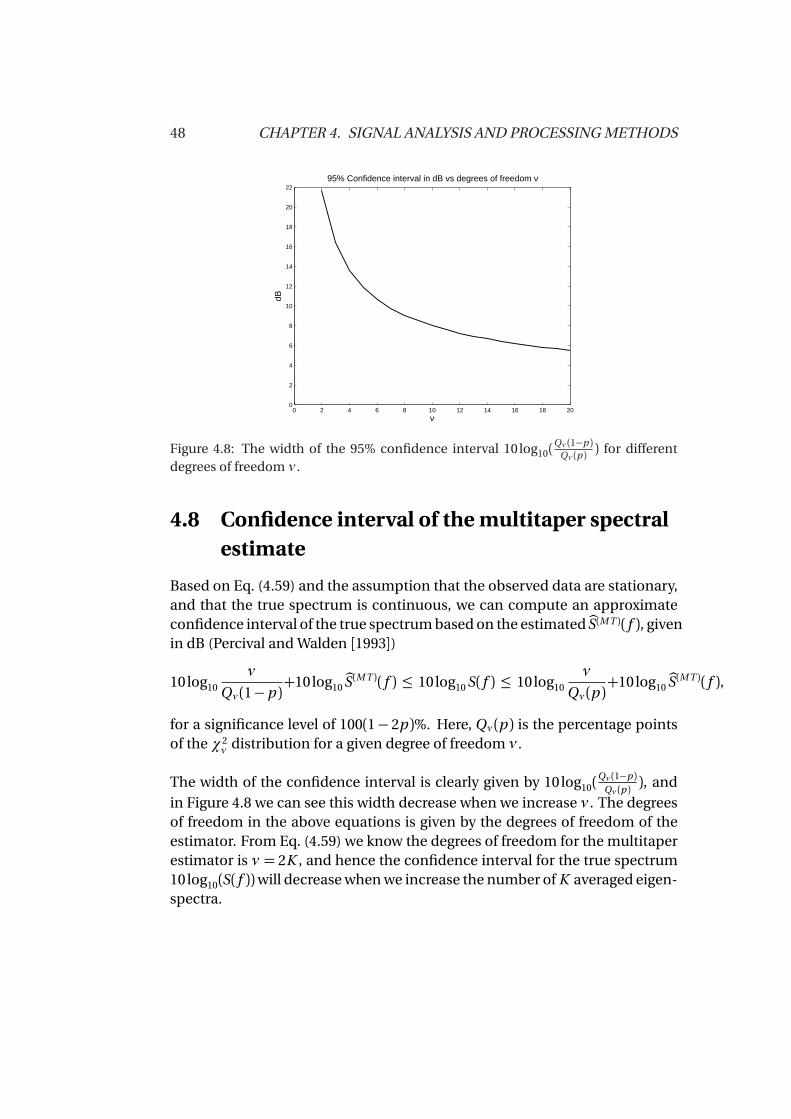
48 CHAPTER 4. SIGNAL ANALYSIS AND PROCESSING METHODS
0 2 4 6 8 10 12 14 16 18 200
2
4
6
8
10
12
14
16
18
20
2295% Confidence interval in dB vs degrees of freedom ν
ν
dB
Figure 4.8: The width of the 95% confidence interval 10 log10(Qν (1−p )
Qν (p )) for different
degrees of freedom ν .
4.8 Confidence interval of the multitaper spectralestimate
Based on Eq. (4.59) and the assumption that the observed data are stationary,and that the true spectrum is continuous, we can compute an approximateconfidence interval of the true spectrum based on the estimated bS(M T )( f ), givenin dB (Percival and Walden [1993])
10log10
ν
Qν (1−p )+10 log10
bS(M T )( f ) ≤ 10log10 S( f ) ≤ 10log10
ν
Qν (p )+10log10
bS(M T )( f ),
for a significance level of 100(1− 2p )%. Here, Qν (p ) is the percentage pointsof the χ2
ν distribution for a given degree of freedom ν .
The width of the confidence interval is clearly given by 10 log10(Qν (1−p )
Qν (p )), and
in Figure 4.8 we can see this width decrease when we increase ν . The degreesof freedom in the above equations is given by the degrees of freedom of theestimator. From Eq. (4.59) we know the degrees of freedom for the multitaperestimator is ν = 2K , and hence the confidence interval for the true spectrum10log10(S( f ))will decrease when we increase the number of K averaged eigen-spectra.
4.9. THOMSON’S F -TEST FOR SINGLE FREQUENCY COMPONENTS 49
4.9 Thomson’s F -test for single frequencycomponents
To test the observed data for spectral lines (sinusoidal components), Thom-son [1982] proposed a F -test to check the significance of possible present sin-gle frequency components. We will now describe the test, closely followingthe approach from Percival and Walden [1993](p.496).
The observed data are now assumed to contain one sinusoidal componentsat a given frequency f i
XS[n ] =Di cos(2π f i n∆t +φi )+ε[n ]. (4.60)
Here, the part ε[n ] represents the background noise, assumed to have a con-tinuous spectrum, and is "locally white" in the frequency band [ f i−W, f i+W ].We recall that 2W is the width of the mainlobe of the spectral window whenusing the multitaper method with DPSS windows. For a given frequency, theexpectation value of the observed data equals the sinusoidal part,
E XS[n ]=Di cos(2π f i n∆t +φi ) =C i e i 2π f i n∆t +C ∗i e−i 2π f i n∆t ,
where ∗ denotes the complex conjugate, and C i = (Di/2)e iφi . The observeddata can then be written as XS[n ] = E XS[n ]+ε[n ].
We rewrite the eigenspectrum from Eq. (4.40), and include the scaling in theabsolute sign
bSk ( f ) =Jk ( f )
2 ,
where we define Jk ( f ) as
Jk ( f ) = (∆t )1/2N−1∑
n=0
vk [n ]XS[n ]e−i 2π f n∆t , (4.61)
where vk [n ] is the k ’th order DPSS window function. For f = f i and 2 f i >W ,Jk ( f i ) can be approximated as
Jk ( f i )≈C iVk (0)
(∆t )1/2+(∆t )1/2
N−1∑
n=0
vk [n ]ε[n ]e−i 2π f i n∆t , (4.62)
where Vk ( f ) is the discrete time Fourier transform of the k ’th order DPSS func-tion Vk ( f ) = ∆t
∑N−1n=0 vk [n ]e−i 2π f n∆t . The first term in Eq. (4.62) is the contri-
bution from the sinusoidal component, and the last term represents the back-ground noise, which is the nature of the true background spectrum, denoted
50 CHAPTER 4. SIGNAL ANALYSIS AND PROCESSING METHODS
by Sε( f ).
By linear regression an estimator of C i can be found as
cC i = (∆t )1/2∑K−1
k=0 Jk ( f i )Vk (0)∑K−1k=0 V 2
k (0). (4.63)
Under the null hypothesis,cC i ( f i ) is assumed to be a zero mean complex Gaus-sian variable, and |cC i ( f i )|2 will be a sum of two squared independent variables,were each part has the variance Sε( f i )∆t /2
∑K−1k=0 V 2
k (0). A scaled |cC i ( f i )|2 vari-able will then follow a chi-square distribution with 2 degrees of freedom
2|cC i |2∑K−1
k=0 V 2k (0)
Sε( f i )∆td=χ2
2 . (4.64)
We can now form an estimate of the background spectrum by subtracting thecontribution from the sinusoidal part in Eq. (4.62), using the estimated cC i ,and perform a multitaper estimate on the residuals
bS(M T )ε ( f i ) =
1
K
K−1∑
k=0
Jk ( f i )−cC iVk (0)
(∆t )1/2
2
. (4.65)
As given in Eq. (4.59), the multitaper estimate has a scaled chi-square distribu-tion with 2K degrees of freedom, but the subtraction including bC i in Eq. (4.65)reduces the sum of squared independent variables by 2. The scaled variablebS(M T )ε ( f i ) therefore follows a chi-square distribution with 2K − 2 degrees of
freedom,
2K bS(M T )ε ( f i )
Sε( f i )=
2∑K−1
k=0
Jk ( f i )−cC iVk (0)(∆t )1/2
2
Sε( f i )d=χ2
2K−2. (4.66)
Finally, the F -test proposed by Thomson is formed by the ratio between thetwo chi-square variables in Eq. (4.64) and Eq. (4.66), divided by their respec-tive degrees of freedom, giving a new F -distributed variable with 2 and 2K −2degrees of freedom, respectively:
2|cC i |2∑K−1k=0 V 2
k (0)
Sε( f i )∆t/2
2K bS(M T )ε ( f i )
Sε( f i )/ (2K −2)
d= F2,2K−2.
Rearranging, the basic quantity that should be calculated is given by
F ( f i ) =(K −1)
cC i
2∑K−1
k=0 V 2k (0)
∆t∑K−1
k=0
Jk ( f i )−cC iVk (0)(∆t )1/2
2 . (4.67)
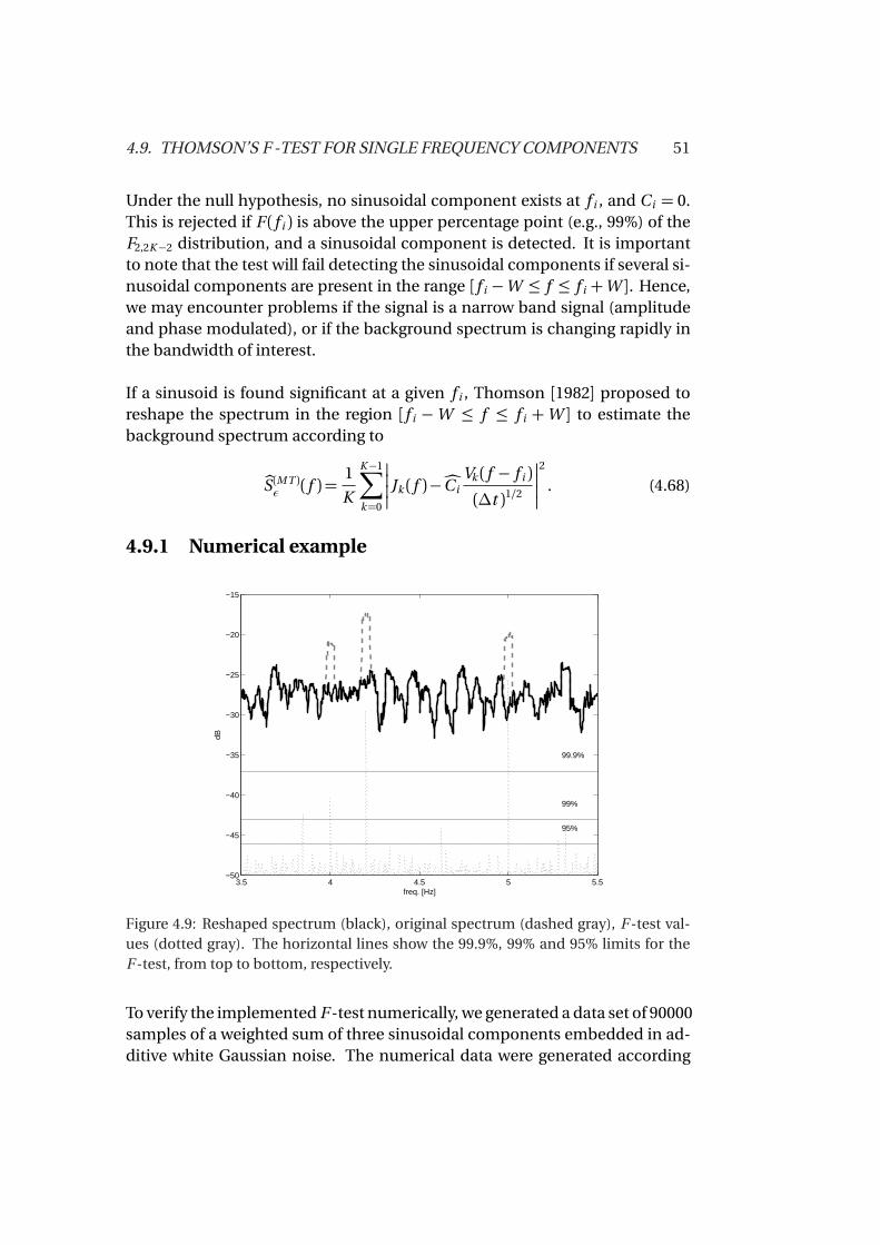
4.9. THOMSON’S F -TEST FOR SINGLE FREQUENCY COMPONENTS 51
Under the null hypothesis, no sinusoidal component exists at f i , and C i = 0.This is rejected if F ( f i ) is above the upper percentage point (e.g., 99%) of theF2,2K−2 distribution, and a sinusoidal component is detected. It is importantto note that the test will fail detecting the sinusoidal components if several si-nusoidal components are present in the range [ f i −W ≤ f ≤ f i +W ]. Hence,we may encounter problems if the signal is a narrow band signal (amplitudeand phase modulated), or if the background spectrum is changing rapidly inthe bandwidth of interest.
If a sinusoid is found significant at a given f i , Thomson [1982] proposed toreshape the spectrum in the region [ f i −W ≤ f ≤ f i +W ] to estimate thebackground spectrum according to
bS(M T )ε ( f ) =
1
K
K−1∑
k=0
Jk ( f )−cC iVk ( f − f i )
(∆t )1/2
2
. (4.68)
4.9.1 Numerical example
3.5 4 4.5 5 5.5−50
−45
−40
−35
−30
−25
−20
−15
95%
99%
99.9%
freq. [Hz]
dB
Figure 4.9: Reshaped spectrum (black), original spectrum (dashed gray), F -test val-ues (dotted gray). The horizontal lines show the 99.9%, 99% and 95% limits for theF -test, from top to bottom, respectively.
To verify the implemented F -test numerically, we generated a data set of 90000samples of a weighted sum of three sinusoidal components embedded in ad-ditive white Gaussian noise. The numerical data were generated according
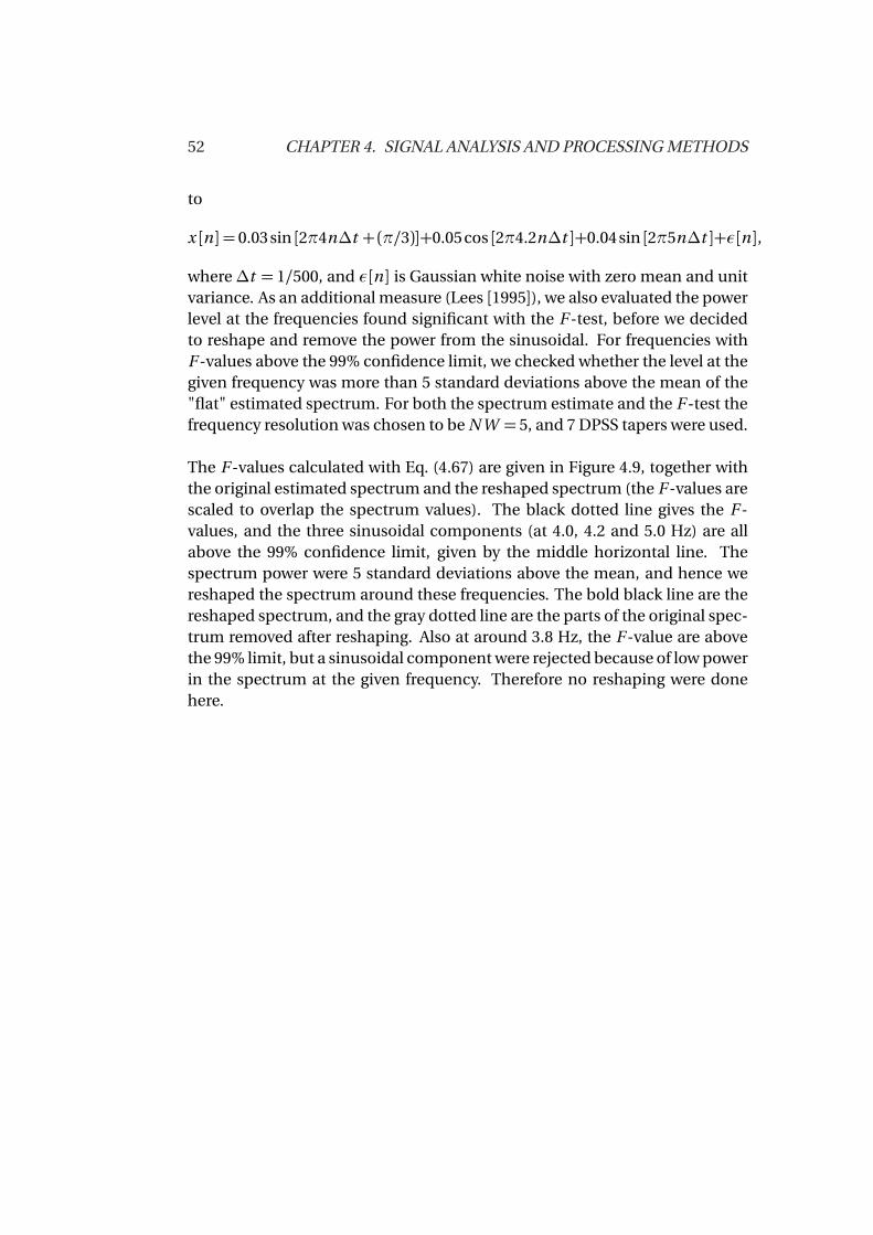
52 CHAPTER 4. SIGNAL ANALYSIS AND PROCESSING METHODS
to
x [n ] = 0.03 sin [2π4n∆t +(π/3)]+0.05 cos [2π4.2n∆t ]+0.04sin [2π5n∆t ]+ε[n ],
where∆t = 1/500, and ε[n ] is Gaussian white noise with zero mean and unitvariance. As an additional measure (Lees [1995]), we also evaluated the powerlevel at the frequencies found significant with the F -test, before we decidedto reshape and remove the power from the sinusoidal. For frequencies withF -values above the 99% confidence limit, we checked whether the level at thegiven frequency was more than 5 standard deviations above the mean of the"flat" estimated spectrum. For both the spectrum estimate and the F -test thefrequency resolution was chosen to be N W = 5, and 7 DPSS tapers were used.
The F -values calculated with Eq. (4.67) are given in Figure 4.9, together withthe original estimated spectrum and the reshaped spectrum (the F -values arescaled to overlap the spectrum values). The black dotted line gives the F -values, and the three sinusoidal components (at 4.0, 4.2 and 5.0 Hz) are allabove the 99% confidence limit, given by the middle horizontal line. Thespectrum power were 5 standard deviations above the mean, and hence wereshaped the spectrum around these frequencies. The bold black line are thereshaped spectrum, and the gray dotted line are the parts of the original spec-trum removed after reshaping. Also at around 3.8 Hz, the F -value are abovethe 99% limit, but a sinusoidal component were rejected because of low powerin the spectrum at the given frequency. Therefore no reshaping were donehere.
Chapter 5
Results
5.1 E-field measurements: 50 m cable antenna,Station 1
The following analysis will be conducted on data from the vertical electricfield measured by the 50 m long cable antenna located at Station 1 (see Figure3.2). A total of 900000 samples were recorded at the sampling rate f s = 500 Hz,giving a total of 30 minutes of data. As the antenna actually measured thevoltage between the electrodes, the electric field were obtained by dividingthe voltage by the length of the cable. Hence, the source of the motion in-duced electric field is the average apparent water velocity between the elec-trodes. Since we are interested in the fluctuation of the E -field in the range0.1-10 Hz, the overall sample mean was removed before further analysis (x =−22.8 µV/m). Note that the DC-level for the electrode pair was not absolutelycalibrated (Blixt [2007]), and we will not relate this mean level to the meanwater velocity (East-West).
5.1.1 Time series
The time series of the analysed data is given in Figure 5.1. Two main featuresare observed, an overall trend, and a prominent oscillation with a modulatedamplitude. The first minute of the data is plotted in the upper right corner,and clearly shows the oscillation. Here we can also count about 9 cycles dur-ing the 60 seconds, giving an oscillation frequency about 0.15 Hz and periodT ≈ 6.7 s.
We received weather data from a nearby platform (Meteorologisk institutt [2007]),and during the electric field recordings, the average frequency of the surface
53
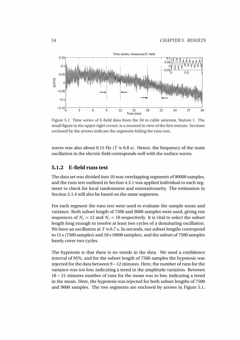
54 CHAPTER 5. RESULTS
0 3 6 9 12 15 18 21 24 27 30−0.15
−0.1
−0.05
0
0.05
0.1
0.15
Time [min]
[µV
/m]
Time series, measured E−field
0 0.5 1−0.05
00.050.1
Figure 5.1: Time series of E-field data from the 50 m cable antenna, Station 1. Thesmall figure in the upper right corner, is a zoomed in view of the first minute. Sectionsenclosed by the arrows indicate the segments failing the runs test.
waves was also about 0.15 Hz (T ≈ 6.8 s). Hence, the frequency of the mainoscillation in the electric field corresponds well with the surface waves.
5.1.2 E-field runs test
The data set was divided into 10 non-overlapping segments of 90000 samples,and the runs test outlined in Section 4.3.1 was applied individual to each seg-ment to check for local randomness and nonstationarity. The estimation inSection 5.1.4 will also be based on the same segments.
For each segment the runs test were used to evaluate the sample mean andvariance. Both subset length of 7500 and 9000 samples were used, giving runsequences of Ns = 12 and Ns = 10 respectively. It is vital to select the subsetlength long enough to resolve at least two cycles of a dominating oscillation.We have an oscillation at T ≈ 6.7 s. In seconds, our subset lengths correspondto 15 s (7500 samples) and 18 s (9000 samples), and the subset of 7500 samplesbarely cover two cycles.
The hypotesis is that there is no trends in the data. We used a confidenceinterval of 95%, and for the subset length of 7500 samples the hypotesis wasrejected for the data between 9−12 minutes. Here, the number of runs for thevariance was too low, indicating a trend in the amplitude variation. Between18− 21 minutes number of runs for the mean was to low, indicating a trendin the mean. Here, the hypotesis was rejected for both subset lengths of 7500and 9000 samples. The two segments are enclosed by arrows in Figure 5.1,
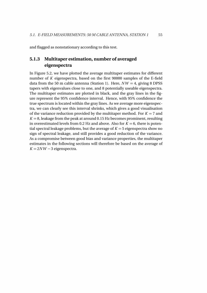
5.1. E-FIELD MEASUREMENTS: 50 M CABLE ANTENNA, STATION 1 55
and flagged as nonstationary according to this test.
5.1.3 Multitaper estimation, number of averagedeigenspectra
In Figure 5.2, we have plotted the average multitaper estimates for differentnumber of K eigenspectra, based on the first 90000 samples of the E-fielddata from the 50 m cable antenna (Station 1). Here, N W = 4, giving 8 DPSStapers with eigenvalues close to one, and 8 potentially useable eigenspectra.The multitaper estimates are plotted in black, and the gray lines in the fig-ure represent the 95% confidence interval. Hence, with 95% confidence thetrue spectrum is located within the gray lines. As we average more eigenspec-tra, we can clearly see this interval shrinks, which gives a good visualisationof the variance reduction provided by the multitaper method. For K = 7 andK = 8, leakage from the peak at around 0.15 Hz becomes prominent, resultingin overestimated levels from 0.2 Hz and above. Also for K = 6, there is poten-tial spectral leakage problems, but the average of K = 5 eigenspectra show nosign of spectral leakage, and still provides a good reduction of the variance.As a compromise between good bias and variance properties, the multitaperestimates in the following sections will therefore be based on the average ofK = 2N W −3 eigenspectra.
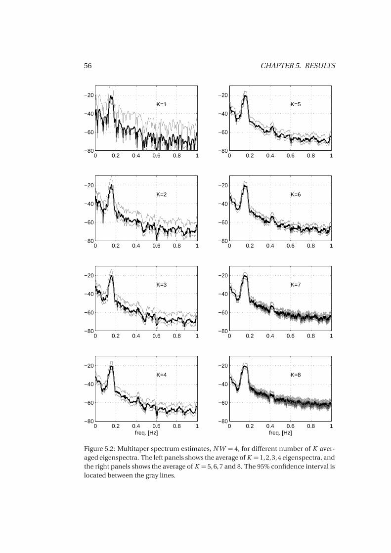
56 CHAPTER 5. RESULTS
0 0.2 0.4 0.6 0.8 1−80
−60
−40
−20
K=1
0 0.2 0.4 0.6 0.8 1−80
−60
−40
−20
K=2
0 0.2 0.4 0.6 0.8 1−80
−60
−40
−20
K=3
0 0.2 0.4 0.6 0.8 1−80
−60
−40
−20
K=4
freq. [Hz]
0 0.2 0.4 0.6 0.8 1−80
−60
−40
−20
K=5
0 0.2 0.4 0.6 0.8 1−80
−60
−40
−20
K=6
0 0.2 0.4 0.6 0.8 1−80
−60
−40
−20
K=7
0 0.2 0.4 0.6 0.8 1−80
−60
−40
−20
K=8
freq. [Hz]
Figure 5.2: Multitaper spectrum estimates, N W = 4, for different number of K aver-aged eigenspectra. The left panels shows the average of K = 1, 2, 3, 4 eigenspectra, andthe right panels shows the average of K = 5, 6, 7 and 8. The 95% confidence interval islocated between the gray lines.
5.1. E-FIELD MEASUREMENTS: 50 M CABLE ANTENNA, STATION 1 57
5.1.4 Time series, spectral estimates and probability densityfunction estimates
To study the development of the vertical electric field with time, the analysisin this Section is based on 3 minutes long data segments (N = 90000 samples).The power spectrum density (PSD) and the probability density function (PDF)were estimated by the methods outlined in Section 4.5.2 and 4.2 respectively.The multitaper method is more robust against nonstationary data than singlewindowed methods, and the time length of the used data segments are alsoshort. Therefore, also the segments found nonstationary in Section 5.1.2, willbe included in this analysis. The region of interest is 0.1-10 Hz, and the spec-trum estimates in this section only displays the interval between 0-10 Hz.
The time series with the sample mean removed are presented in Figure 5.3,5.4, 5.5, 5.6 and 5.7, together with spectrum estimates and PDF estimates foreach segment. Here, each figure contains results for two segments, one ineach column. The upper panels displays the time series of the evaluated data,and the corresponding estimates are aligned below the time series plot. Thespectrum estimates are given in the first and second panels below the timeseries panel, where the uppermost of them gives a zoomed view of the range0−1 Hz, and the next shows the 0−10 Hz range. To reveal consistent featuresin the spectrum estimates, several MT estimates with different frequency res-olution were applied and plotted. Here, N W = 3, 4,5 were used and given inHz, the respective frequency resolutions are approximately 0.033, 0.044 and0.056 Hz. The number of averaged eigenspectra were K = 3, 5,7 respectively.The bottom panels show the estimated probability density functions. Foreach data segment, three estimates with different binwidth b of the Gaussiankernel (see Eq. (4.8)) are plotted in black. Here, b denotes the binwidth givenin Eq. (4.9) and the respective binwidths are b , 2b and 0.1b . For reference, aGaussian distribution function shaped by the sample mean (x ) and the stan-dard deviation (bσ) of the evaluated data is plotted (solid gray) together withthe PDF estimates.
From the time series the most prominent oscillation is clearly visible. By count-ing the cycles in Figure 5.1, we found this oscillation to be around 0.15 Hz. Inthe 0-1 Hz spectrum estimates in Figure 5.3, 5.4, 5.5, 5.6 and 5.7, the main peakhas its maximum around 0.15 Hz for all the time intervals, but we can see thepeakiness, width and level changing during time. Between 0-3 minutes thepeak is at its maximum, between 3-9 minutes the peak gets wider with a lowermaximum. The oscillation amplitude variations seen in the time series, andthe changes in the width of the corresponding peak in the spectrum estimate,
58 CHAPTER 5. RESULTS
indicates that the oscillation is not sinusoidal, but rather an amplitude andpossibly a phase modulated narrow band signal. From 9-30 minutes addi-tional local maxima are developed around the main peak, seen as a shoul-der just above 0.1 Hz, and a feature just below 0.25 Hz which develops into aseparate peak between 24-27 minutes, seen in Figure 5.7. We also observe aconsistent local maximum at just above 0.4 Hz. In the 0-10 Hz plot consistentpeaks are observed at 2, 4 and 5 Hz for all time intervals. Peaks around 6 Hzare most evident in Figure 5.4 and 5.5.
While the main peak corresponds to the mean frequency of the surface wavesat around 0.15 Hz, the maximum around 0.1 Hz correspond to the average fre-quency of the maximum surface waves, with a period of T ≈ 8.48 s and a fre-quency of around 0.12 Hz (Meteorologisk institutt [2007]). The peak around0.25 Hz then corresponds closely to the double frequency of the maximumsurface waves.
The estimates of the probability density (PDF) are displayed in the lower pan-els in Figure 5.3, 5.4, 5.5, 5.6 and 5.7. When evaluating these estimates, wealso use the additional information from the sample moments in Table 5.1.The skewness are only positive for the time intervals 9-12 minutes and 18-21 minutes. These intervals were found nonstationary with the runs test, butfor all the other intervals the skewness is negative. This indicates a left-skeweddistribution, with more data in the left tail compared to Gaussian distributeddata. This is also evident in the figures, where the estimated PDF are abovethe left tail of the Gaussian curve (bold gray). For all time intervals expect 18-21 minutes the kurtosis is also negative (see Table 5.1), and we can see theextreme points of the estimated PDF tails are below the Gaussian (bold gray).This indicates a sub-Gaussian distribution, which describe distributions witha more flat top and lighter tails compared to a Gaussian distribution with thesame mean and variance. In general, if we exclude the time intervals foundnonstationary with the runs test, the distribution of the data are not symmet-ric, but have a left-skewed (negative skewness) distribution, and can also bedescribed as sub-Gaussian because of the light tails and negative kurtosis.
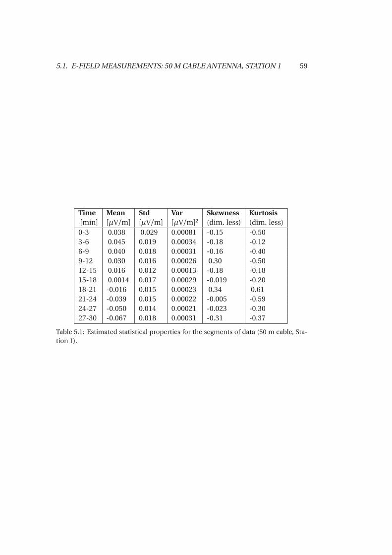
5.1. E-FIELD MEASUREMENTS: 50 M CABLE ANTENNA, STATION 1 59
Time Mean Std Var Skewness Kurtosis[min] [µV/m] [µV/m] [µV/m]2 (dim. less) (dim. less)
0-3 0.038 0.029 0.00081 -0.15 -0.503-6 0.045 0.019 0.00034 -0.18 -0.126-9 0.040 0.018 0.00031 -0.16 -0.409-12 0.030 0.016 0.00026 0.30 -0.5012-15 0.016 0.012 0.00013 -0.18 -0.1815-18 0.0014 0.017 0.00029 -0.019 -0.2018-21 -0.016 0.015 0.00023 0.34 0.6121-24 -0.039 0.015 0.00022 -0.005 -0.5924-27 -0.050 0.014 0.00021 -0.023 -0.3027-30 -0.067 0.018 0.00031 -0.31 -0.37
Table 5.1: Estimated statistical properties for the segments of data (50 m cable, Sta-tion 1).
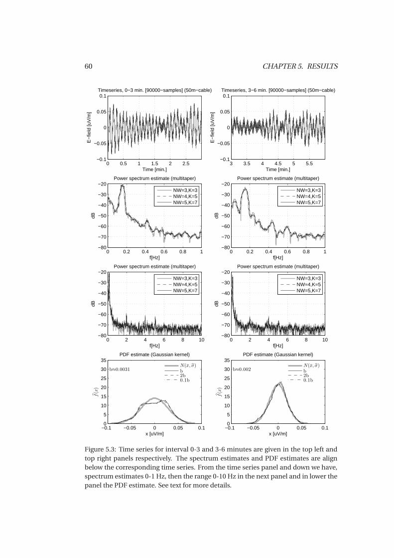
60 CHAPTER 5. RESULTS
0 0.5 1 1.5 2 2.5−0.1
−0.05
0
0.05
0.1
Time [min.]
E−
field
[uV
/m]
Timeseries, 0−3 min. [90000−samples] (50m−cable)
0 0.2 0.4 0.6 0.8 1−80
−70
−60
−50
−40
−30
−20
dB
f[Hz]
Power spectrum estimate (multitaper)
NW=3,K=3NW=4,K=5NW=5,K=7
0 2 4 6 8 10−80
−70
−60
−50
−40
−30
−20
dB
f[Hz]
Power spectrum estimate (multitaper)
NW=3,K=3NW=4,K=5NW=5,K=7
−0.1 −0.05 0 0.05 0.10
5
10
15
20
25
30
35
x [uV/m]
f(x
)
PDF estimate (Gaussian kernel)
b≈0.0031N(x, σ)b2b0.1b
3 3.5 4 4.5 5 5.5−0.1
−0.05
0
0.05
0.1
Time [min.]
E−
field
[uV
/m]
Timeseries, 3−6 min. [90000−samples] (50m−cable)
0 0.2 0.4 0.6 0.8 1−80
−70
−60
−50
−40
−30
−20
dB
f[Hz]
Power spectrum estimate (multitaper)
NW=3,K=3NW=4,K=5NW=5,K=7
0 2 4 6 8 10−80
−70
−60
−50
−40
−30
−20
dB
f[Hz]
Power spectrum estimate (multitaper)
NW=3,K=3NW=4,K=5NW=5,K=7
−0.1 −0.05 0 0.05 0.10
5
10
15
20
25
30
35
x [uV/m]
f(x
)
PDF estimate (Gaussian kernel)
b≈0.002N(x, σ)b2b0.1b
Figure 5.3: Time series for interval 0-3 and 3-6 minutes are given in the top left andtop right panels respectively. The spectrum estimates and PDF estimates are alignbelow the corresponding time series. From the time series panel and down we have,spectrum estimates 0-1 Hz, then the range 0-10 Hz in the next panel and in lower thepanel the PDF estimate. See text for more details.
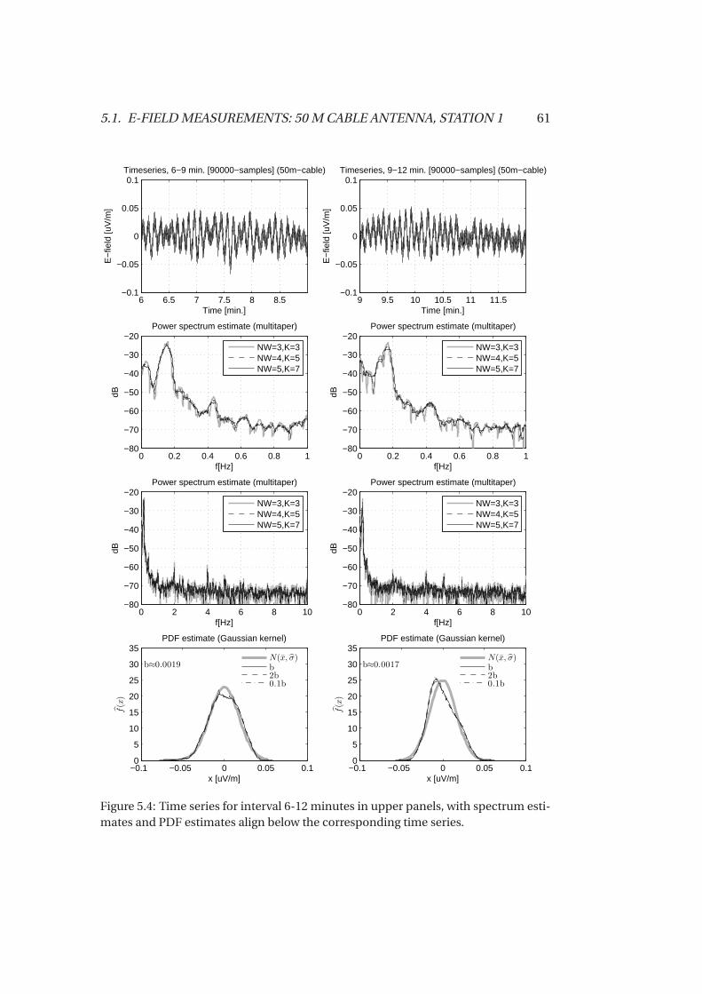
5.1. E-FIELD MEASUREMENTS: 50 M CABLE ANTENNA, STATION 1 61
6 6.5 7 7.5 8 8.5−0.1
−0.05
0
0.05
0.1
Time [min.]
E−
field
[uV
/m]
Timeseries, 6−9 min. [90000−samples] (50m−cable)
0 0.2 0.4 0.6 0.8 1−80
−70
−60
−50
−40
−30
−20
dB
f[Hz]
Power spectrum estimate (multitaper)
0 2 4 6 8 10−80
−70
−60
−50
−40
−30
−20
dB
f[Hz]
Power spectrum estimate (multitaper)
−0.1 −0.05 0 0.05 0.10
5
10
15
20
25
30
35
x [uV/m]
f(x
)
PDF estimate (Gaussian kernel)
b≈0.0019
9 9.5 10 10.5 11 11.5−0.1
−0.05
0
0.05
0.1
Time [min.]
E−
field
[uV
/m]
Timeseries, 9−12 min. [90000−samples] (50m−cable)
0 0.2 0.4 0.6 0.8 1−80
−70
−60
−50
−40
−30
−20dB
f[Hz]
Power spectrum estimate (multitaper)
0 2 4 6 8 10−80
−70
−60
−50
−40
−30
−20
dB
f[Hz]
Power spectrum estimate (multitaper)
−0.1 −0.05 0 0.05 0.10
5
10
15
20
25
30
35
x [uV/m]
f(x
)
PDF estimate (Gaussian kernel)
b≈0.0017
NW=3,K=3NW=4,K=5NW=5,K=7
NW=3,K=3NW=4,K=5NW=5,K=7
N(x, σ)b2b0.1b
NW=3,K=3NW=4,K=5NW=5,K=7
NW=3,K=3NW=4,K=5NW=5,K=7
N(x, σ)b2b0.1b
Figure 5.4: Time series for interval 6-12 minutes in upper panels, with spectrum esti-mates and PDF estimates align below the corresponding time series.
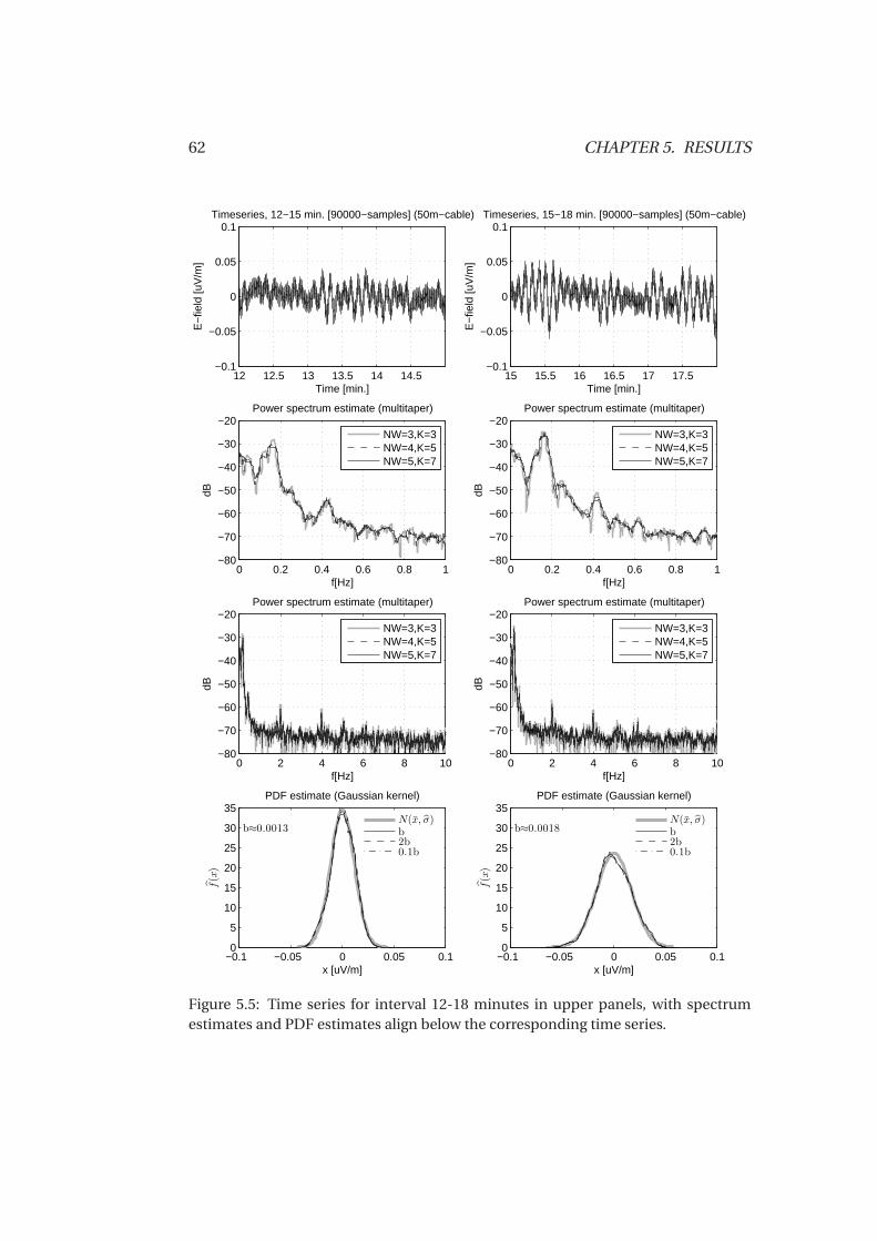
62 CHAPTER 5. RESULTS
12 12.5 13 13.5 14 14.5−0.1
−0.05
0
0.05
0.1
Time [min.]
E−
field
[uV
/m]
Timeseries, 12−15 min. [90000−samples] (50m−cable)
0 0.2 0.4 0.6 0.8 1−80
−70
−60
−50
−40
−30
−20
dB
f[Hz]
Power spectrum estimate (multitaper)
0 2 4 6 8 10−80
−70
−60
−50
−40
−30
−20
dB
f[Hz]
Power spectrum estimate (multitaper)
−0.1 −0.05 0 0.05 0.10
5
10
15
20
25
30
35
x [uV/m]
f(x
)
PDF estimate (Gaussian kernel)
b≈0.0013
15 15.5 16 16.5 17 17.5−0.1
−0.05
0
0.05
0.1
Time [min.]
E−
field
[uV
/m]
Timeseries, 15−18 min. [90000−samples] (50m−cable)
0 0.2 0.4 0.6 0.8 1−80
−70
−60
−50
−40
−30
−20
dB
f[Hz]
Power spectrum estimate (multitaper)
0 2 4 6 8 10−80
−70
−60
−50
−40
−30
−20
dB
f[Hz]
Power spectrum estimate (multitaper)
−0.1 −0.05 0 0.05 0.10
5
10
15
20
25
30
35
x [uV/m]
f(x
)
PDF estimate (Gaussian kernel)
b≈0.0018
NW=3,K=3NW=4,K=5NW=5,K=7
NW=3,K=3NW=4,K=5NW=5,K=7
N(x, σ)b2b0.1b
NW=3,K=3NW=4,K=5NW=5,K=7
NW=3,K=3NW=4,K=5NW=5,K=7
N(x, σ)b2b0.1b
Figure 5.5: Time series for interval 12-18 minutes in upper panels, with spectrumestimates and PDF estimates align below the corresponding time series.
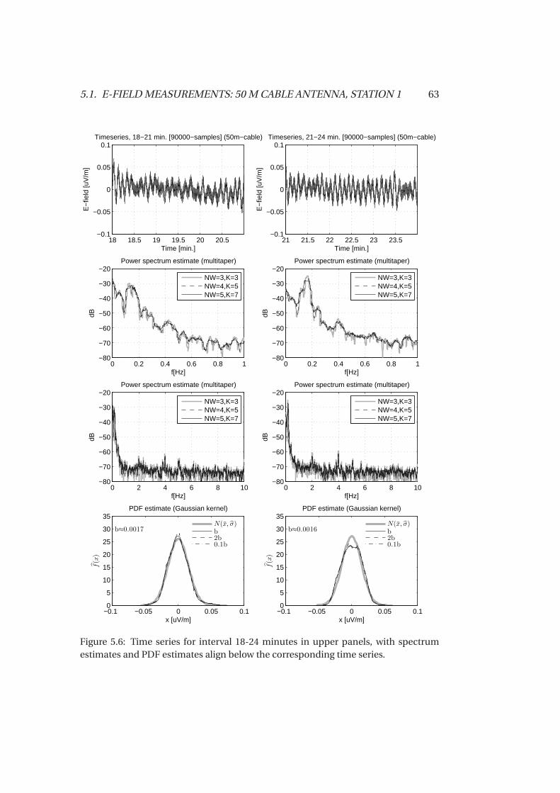
5.1. E-FIELD MEASUREMENTS: 50 M CABLE ANTENNA, STATION 1 63
18 18.5 19 19.5 20 20.5−0.1
−0.05
0
0.05
0.1
Time [min.]
E−
field
[uV
/m]
Timeseries, 18−21 min. [90000−samples] (50m−cable)
0 0.2 0.4 0.6 0.8 1−80
−70
−60
−50
−40
−30
−20
dB
f[Hz]
Power spectrum estimate (multitaper)
0 2 4 6 8 10−80
−70
−60
−50
−40
−30
−20
dB
f[Hz]
Power spectrum estimate (multitaper)
−0.1 −0.05 0 0.05 0.10
5
10
15
20
25
30
35
x [uV/m]
f(x
)
PDF estimate (Gaussian kernel)
b≈0.0017
21 21.5 22 22.5 23 23.5−0.1
−0.05
0
0.05
0.1
Time [min.]
E−
field
[uV
/m]
Timeseries, 21−24 min. [90000−samples] (50m−cable)
0 0.2 0.4 0.6 0.8 1−80
−70
−60
−50
−40
−30
−20dB
f[Hz]
Power spectrum estimate (multitaper)
0 2 4 6 8 10−80
−70
−60
−50
−40
−30
−20
dB
f[Hz]
Power spectrum estimate (multitaper)
−0.1 −0.05 0 0.05 0.10
5
10
15
20
25
30
35
x [uV/m]
f(x
)
PDF estimate (Gaussian kernel)
b≈0.0016
NW=3,K=3NW=4,K=5NW=5,K=7
NW=3,K=3NW=4,K=5NW=5,K=7
N(x, σ)b2b0.1b
NW=3,K=3NW=4,K=5NW=5,K=7
NW=3,K=3NW=4,K=5NW=5,K=7
N(x, σ)b2b0.1b
Figure 5.6: Time series for interval 18-24 minutes in upper panels, with spectrumestimates and PDF estimates align below the corresponding time series.
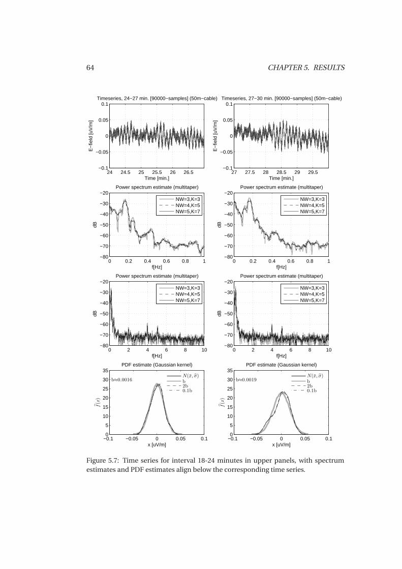
64 CHAPTER 5. RESULTS
24 24.5 25 25.5 26 26.5−0.1
−0.05
0
0.05
0.1
Time [min.]
E−
field
[uV
/m]
Timeseries, 24−27 min. [90000−samples] (50m−cable)
0 0.2 0.4 0.6 0.8 1−80
−70
−60
−50
−40
−30
−20
dB
f[Hz]
Power spectrum estimate (multitaper)
0 2 4 6 8 10−80
−70
−60
−50
−40
−30
−20
dB
f[Hz]
Power spectrum estimate (multitaper)
−0.1 −0.05 0 0.05 0.10
5
10
15
20
25
30
35
x [uV/m]
f(x
)
PDF estimate (Gaussian kernel)
b≈0.0016
27 27.5 28 28.5 29 29.5−0.1
−0.05
0
0.05
0.1
Time [min.]
E−
field
[uV
/m]
Timeseries, 27−30 min. [90000−samples] (50m−cable)
0 0.2 0.4 0.6 0.8 1−80
−70
−60
−50
−40
−30
−20
dB
f[Hz]
Power spectrum estimate (multitaper)
0 2 4 6 8 10−80
−70
−60
−50
−40
−30
−20
dB
f[Hz]
Power spectrum estimate (multitaper)
−0.1 −0.05 0 0.05 0.10
5
10
15
20
25
30
35
x [uV/m]
f(x
)
PDF estimate (Gaussian kernel)
b≈0.0019
NW=3,K=3NW=4,K=5NW=5,K=7
NW=3,K=3NW=4,K=5NW=5,K=7
N(x, σ)b2b0.1b
NW=3,K=3NW=4,K=5NW=5,K=7
NW=3,K=3NW=4,K=5NW=5,K=7
N(x, σ)b2b0.1b
Figure 5.7: Time series for interval 18-24 minutes in upper panels, with spectrumestimates and PDF estimates align below the corresponding time series.
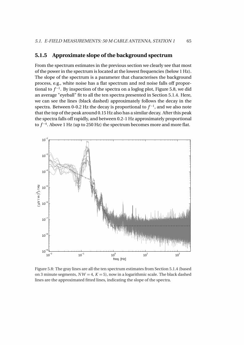
5.1. E-FIELD MEASUREMENTS: 50 M CABLE ANTENNA, STATION 1 65
5.1.5 Approximate slope of the background spectrum
From the spectrum estimates in the previous section we clearly see that mostof the power in the spectrum is located at the lowest frequencies (below 1 Hz).The slope of the spectrum is a parameter that characterises the backgroundprocess, e.g., white noise has a flat spectrum and red noise falls off propor-tional to f −1. By inspection of the spectra on a loglog plot, Figure 5.8, we didan average "eyeball" fit to all the ten spectra presented in Section 5.1.4. Here,we can see the lines (black dashed) approximately follows the decay in thespectra. Between 0-0.2 Hz the decay is proportional to f −1, and we also notethat the top of the peak around 0.15 Hz also has a similar decay. After this peakthe spectra falls off rapidly, and between 0.2-1 Hz approximately proportionalto f −4. Above 1 Hz (up to 250 Hz) the spectrum becomes more and more flat.
10−2
10−1
100
101
102
10−9
10−8
10−7
10−6
10−5
10−4
10−3
10−2
freq. [Hz]
( µV
/ m
)2 )
/ Hz
Figure 5.8: The gray lines are all the ten spectrum estimates from Section 5.1.4 (basedon 3 minute segments, N W = 4, K = 5), now in a logarithmic scale. The black dashedlines are the approximated fitted lines, indicating the slope of the spectra.
66 CHAPTER 5. RESULTS
5.1.6 F -test for sinusoidal components
To search for significant single frequency components, the F -test given in Sec-tion 4.9 was applied to the measured data (50 m cable, Station 1). We con-structed an automatic routine were significant components where detectedbased on the following criteria: 1) Only select frequencies were the F -valuesare above the 99.9% confidence level. 2) For frequencies with F -values abovethe selected confidence limits, the power level for that frequency were thencompared to the mean level of the "flat" region from 1 Hz to 250 Hz. Only fre-quencies with a power level more than 5 standard deviations above this mean,were found significant. For most of the frequencies between DC and 1 Hz, thelevel are above the mean plus 5bσ, and in practice this criterion only affectsthe frequencies above 1 Hz.
The test was applied to the same segments as in Section 5.1.4, and for eachsegment the test was done with different frequency resolutions, N W = 4,5and N W = 6, respectively, and the number DPSS tapers applied were K = 5,6and 7, respectively.
All the significant frequencies from the test are summarised in Figure 5.9, werethe significant components are labeled to show for which resolution the com-ponent were found significant (N W = 4 (•), N W = 5 () and N W = 6 (2)).Clearly, most of the significant components are detected in the range from10 Hz and above, were the spectrum is flattening out. The natural spectrumof the electric field fluctuations, are not expected to contain energetic fea-tures at these frequencies (Filloux [1973]), and the significant peaks are mostlikely caused by the electronics. The peak around 5 Hz, is seen in the spec-trum from both the antenna at Station 1 and Station 2 (data from Station 2will be presented in Section 5.4, Figure 5.19), is related to the electronics (Blixt[2007]), and the bundle of frequency components detected around 20, 60 150and 220 Hz (Figure 5.9) are actually spaced by 5 and 10 Hz. We also note thatthe same frequency components are not significant for all time intervals, indi-cating that the level or the phase of the periodic components vary with time.From 10 Hz and above, only the components at 10 Hz and 155 Hz are signifi-cant in only one test, while the other components are either found significantin several tests for the same data segment (with different resolution), or at dif-ferent time intervals.
Between DC and 10 Hz significant components were detected at 0.16, 0.24,1.0, 2.0, 4.0 and 10.0 Hz. These are summarised in Table 5.2, including thetime interval during which they were detected, and the resolution N W that
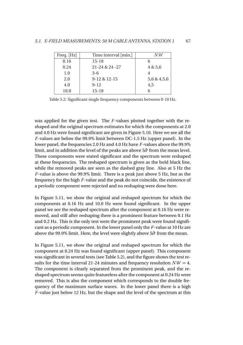
5.1. E-FIELD MEASUREMENTS: 50 M CABLE ANTENNA, STATION 1 67
Freq. [Hz] Time interval [min.] N W0.16 15-18 60.24 21-24 & 24 -27 4 & 5,61.0 3-6 42.0 9-12 & 12-15 5,6 & 4,5,64.0 9-12 4,5
10.0 15-18 6
Table 5.2: Significant single frequency components between 0-10 Hz.
was applied for the given test. The F -values plotted together with the re-shaped and the original spectrum estimates for which the components at 2.0and 4.0 Hz were found significant are given in Figure 5.10. Here we see all theF -values are below the 99.9% limit between DC-1.5 Hz (upper panel). In thelower panel, the frequencies 2.0 Hz and 4.0 Hz have F -values above the 99.9%limit, and in addition the level of the peaks are above 5bσ from the mean level.These components were stated significant and the spectrum were reshapedat these frequencies. The reshaped spectrum is given as the bold black line,while the removed peaks are seen as the dashed gray line. Also at 5 Hz theF -value is above the 99.9% limit. There is a peak just above 5 Hz, but as thefrequency for the high F -value and the peak do not coincide, the existence ofa periodic component were rejected and no reshaping were done here.
In Figure 5.11, we show the original and reshaped spectrum for which thecomponents at 0.16 Hz and 10.0 Hz were found significant. In the upperpanel we see the reshaped spectrum after the component at 0.16 Hz were re-moved, and still after reshaping there is a prominent feature between 0.1 Hzand 0.2 Hz. This is the only test were the prominent peak were found signifi-cant as a periodic component. In the lower panel only the F -value at 10 Hz areabove the 99.9% limit. Here, the level were slightly above 5bσ from the mean.
In Figure 5.11, we show the original and reshaped spectrum for which thecomponent at 0.24 Hz was found significant (upper panel). This componentwas significant in several tests (see Table 5.2), and the figure shows the test re-sults for the time interval 21-24 minutes and frequency resolution N W = 4.The component is clearly separated from the prominent peak, and the re-shaped spectrum seems quite featureless after the component at 0.24 Hz wereremoved. This is also the component which corresponds to the double fre-quency of the maximum surface waves. In the lower panel there is a highF -value just below 12 Hz, but the shape and the level of the spectrum at this
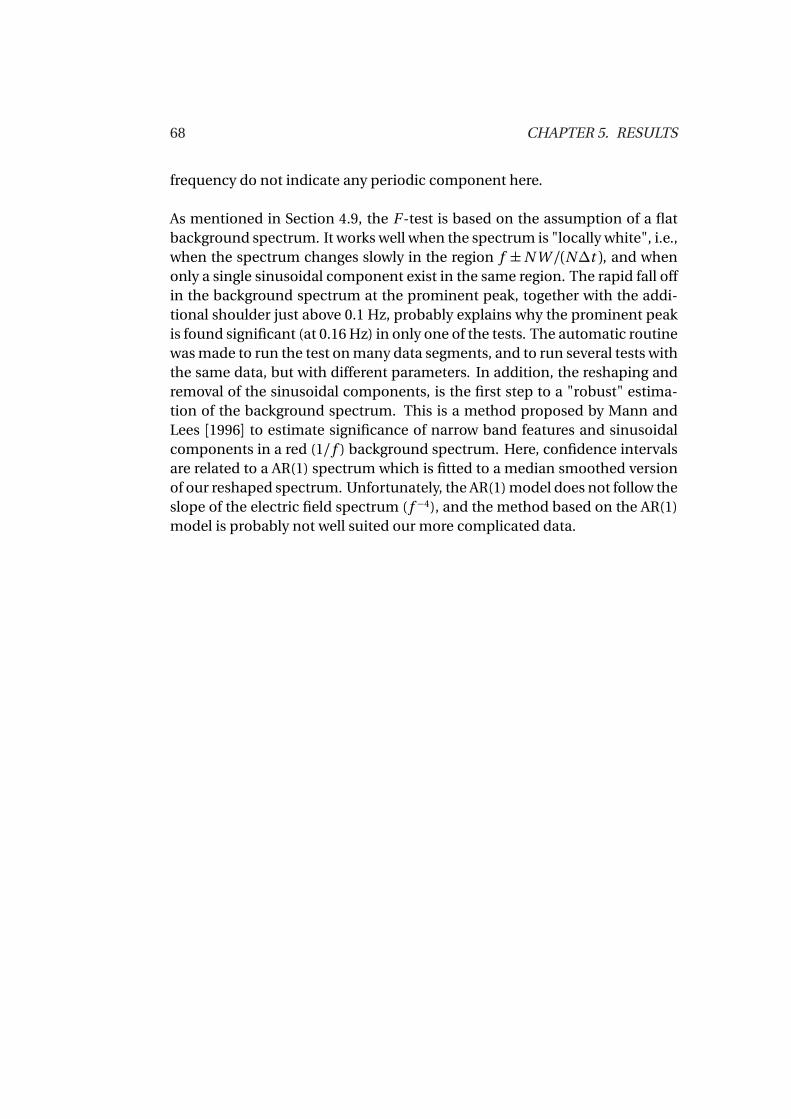
68 CHAPTER 5. RESULTS
frequency do not indicate any periodic component here.
As mentioned in Section 4.9, the F -test is based on the assumption of a flatbackground spectrum. It works well when the spectrum is "locally white", i.e.,when the spectrum changes slowly in the region f ±N W /(N∆t ), and whenonly a single sinusoidal component exist in the same region. The rapid fall offin the background spectrum at the prominent peak, together with the addi-tional shoulder just above 0.1 Hz, probably explains why the prominent peakis found significant (at 0.16 Hz) in only one of the tests. The automatic routinewas made to run the test on many data segments, and to run several tests withthe same data, but with different parameters. In addition, the reshaping andremoval of the sinusoidal components, is the first step to a "robust" estima-tion of the background spectrum. This is a method proposed by Mann andLees [1996] to estimate significance of narrow band features and sinusoidalcomponents in a red (1/ f ) background spectrum. Here, confidence intervalsare related to a AR(1) spectrum which is fitted to a median smoothed versionof our reshaped spectrum. Unfortunately, the AR(1) model does not follow theslope of the electric field spectrum (f −4), and the method based on the AR(1)model is probably not well suited our more complicated data.
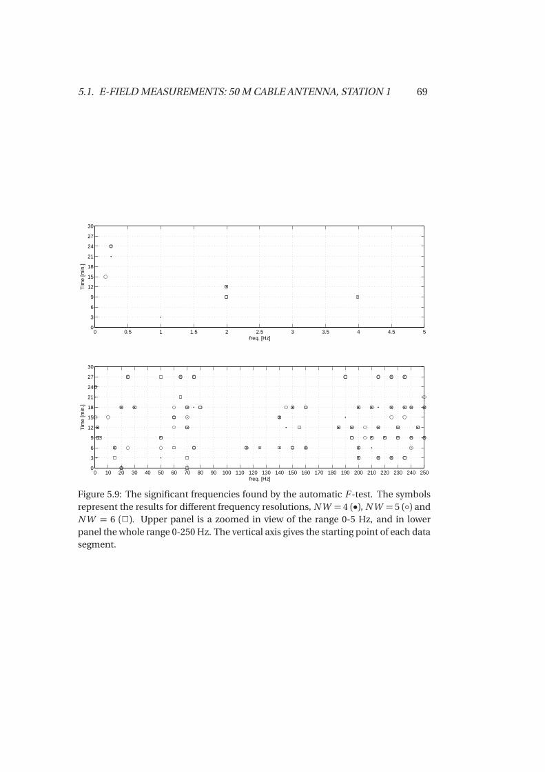
5.1. E-FIELD MEASUREMENTS: 50 M CABLE ANTENNA, STATION 1 69
0 0.5 1 1.5 2 2.5 3 3.5 4 4.5 50
3
6
9
12
15
18
21
24
27
30
freq. [Hz]
Tim
e [m
in.]
0 10 20 30 40 50 60 70 80 90 100 110 120 130 140 150 160 170 180 190 200 210 220 230 240 2500
3
6
9
12
15
18
21
24
27
30
freq. [Hz]
Tim
e [m
in.]
Figure 5.9: The significant frequencies found by the automatic F -test. The symbolsrepresent the results for different frequency resolutions, N W = 4 (•), N W = 5 () andN W = 6 (2). Upper panel is a zoomed in view of the range 0-5 Hz, and in lowerpanel the whole range 0-250 Hz. The vertical axis gives the starting point of each datasegment.
70 CHAPTER 5. RESULTS
0 0.1 0.2 0.3 0.4 0.5 0.6 0.7 0.8 0.9 1 1.1 1.2 1.3 1.4 1.5−90
−80
−70
−60
−50
−40
−30
−20
99% 99.9%
F−test, time interval 9−12 min. (NW = 5 ,K = 7)
freq. [Hz]
dB
2 3 4 5 6 7 8 9 10 11 12−90
−80
−70
−60
−50
−40
99%
99.9%
freq. [Hz]
dB
Figure 5.10: F -test plot with significant components at 2.0 and 4.0 Hz, for the timeinterval 9-12 minutes. The estimated F -values (dotted line) and the 99 and 99.9%confidence limits (solid horizontal lines), are scaled to overlap the spectrum. Thedashed horizontal lines are the mean level between 1-250 Hz (lowermost) and themean level plus 5bσ. The reshaped spectrum are given in bold black and the originalspectrum is in bold dashed gray. The range 0-1.5 Hz and 1.5-12 Hz are given in upperand lower panel respectively.
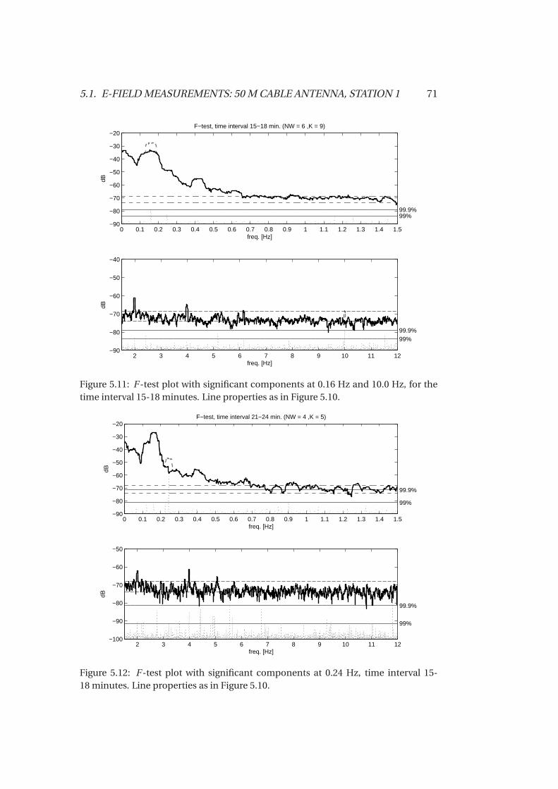
5.1. E-FIELD MEASUREMENTS: 50 M CABLE ANTENNA, STATION 1 71
0 0.1 0.2 0.3 0.4 0.5 0.6 0.7 0.8 0.9 1 1.1 1.2 1.3 1.4 1.5−90
−80
−70
−60
−50
−40
−30
−20
99% 99.9%
F−test, time interval 15−18 min. (NW = 6 ,K = 9)
freq. [Hz]
dB
2 3 4 5 6 7 8 9 10 11 12−90
−80
−70
−60
−50
−40
99% 99.9%
freq. [Hz]
dB
Figure 5.11: F -test plot with significant components at 0.16 Hz and 10.0 Hz, for thetime interval 15-18 minutes. Line properties as in Figure 5.10.
0 0.1 0.2 0.3 0.4 0.5 0.6 0.7 0.8 0.9 1 1.1 1.2 1.3 1.4 1.5−90
−80
−70
−60
−50
−40
−30
−20
99%
99.9%
F−test, time interval 21−24 min. (NW = 4 ,K = 5)
freq. [Hz]
dB
2 3 4 5 6 7 8 9 10 11 12−100
−90
−80
−70
−60
−50
99%
99.9%
freq. [Hz]
dB
Figure 5.12: F -test plot with significant components at 0.24 Hz, time interval 15-18 minutes. Line properties as in Figure 5.10.
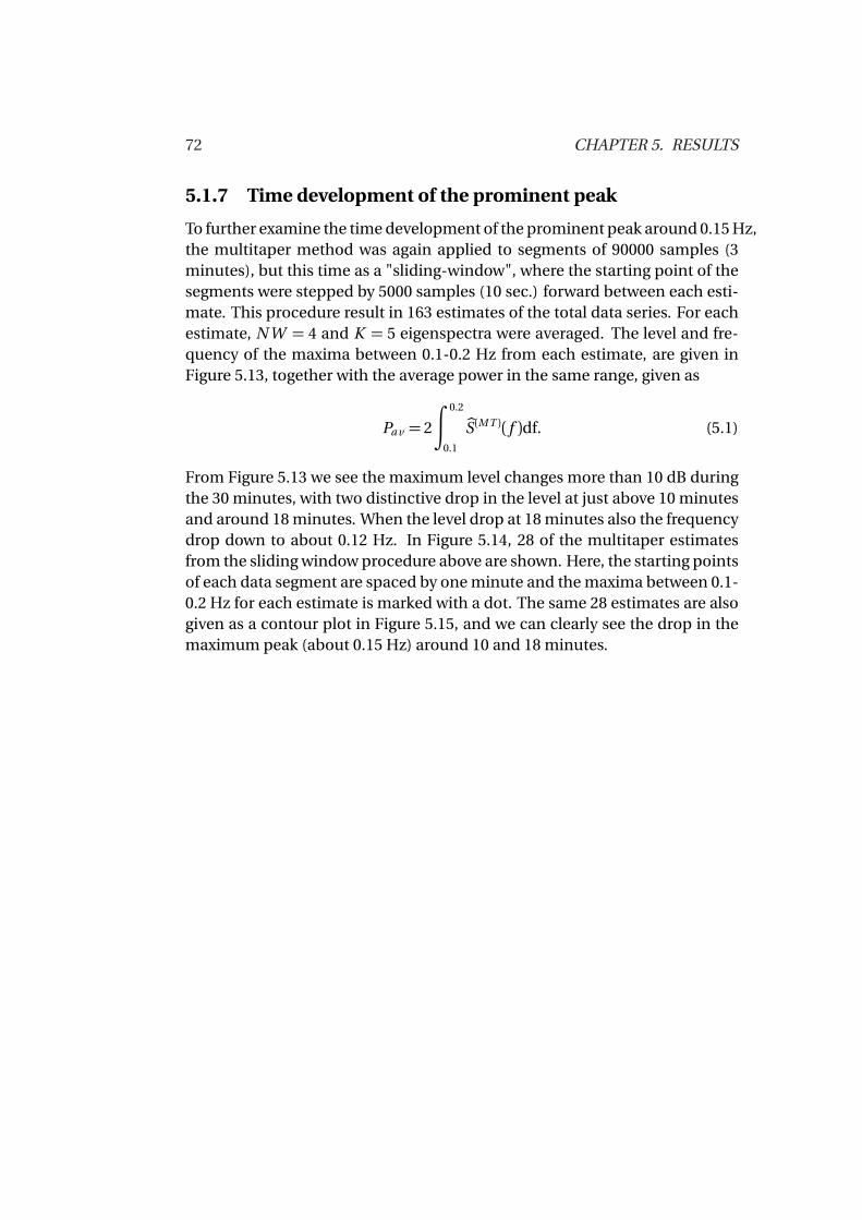
72 CHAPTER 5. RESULTS
5.1.7 Time development of the prominent peak
To further examine the time development of the prominent peak around 0.15 Hz,the multitaper method was again applied to segments of 90000 samples (3minutes), but this time as a "sliding-window", where the starting point of thesegments were stepped by 5000 samples (10 sec.) forward between each esti-mate. This procedure result in 163 estimates of the total data series. For eachestimate, N W = 4 and K = 5 eigenspectra were averaged. The level and fre-quency of the maxima between 0.1-0.2 Hz from each estimate, are given inFigure 5.13, together with the average power in the same range, given as
Pa v = 2
∫ 0.2
0.1
bS(M T )( f )df. (5.1)
From Figure 5.13 we see the maximum level changes more than 10 dB duringthe 30 minutes, with two distinctive drop in the level at just above 10 minutesand around 18 minutes. When the level drop at 18 minutes also the frequencydrop down to about 0.12 Hz. In Figure 5.14, 28 of the multitaper estimatesfrom the sliding window procedure above are shown. Here, the starting pointsof each data segment are spaced by one minute and the maxima between 0.1-0.2 Hz for each estimate is marked with a dot. The same 28 estimates are alsogiven as a contour plot in Figure 5.15, and we can clearly see the drop in themaximum peak (about 0.15 Hz) around 10 and 18 minutes.
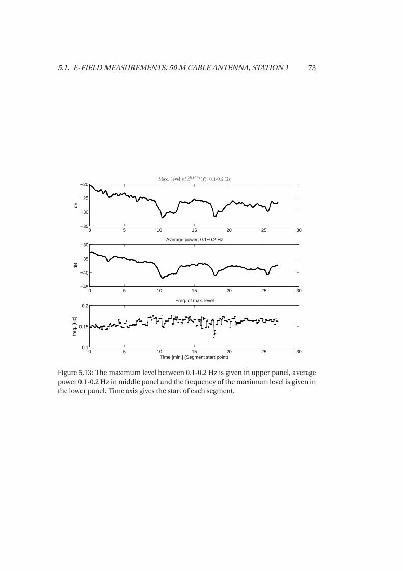
5.1. E-FIELD MEASUREMENTS: 50 M CABLE ANTENNA, STATION 1 73
0 5 10 15 20 25 30−35
−30
−25
−20Max. level of S(MT)(f), 0.1-0.2 Hz
dB
0 5 10 15 20 25 30−45
−40
−35
−30Average power, 0.1−0.2 Hz
dB
0 5 10 15 20 25 300.1
0.15
0.2Freq. of max. level
Time [min.] (Segment start point)
freq
. [H
z]
Figure 5.13: The maximum level between 0.1-0.2 Hz is given in upper panel, averagepower 0.1-0.2 Hz in middle panel and the frequency of the maximum level is given inthe lower panel. Time axis gives the start of each segment.
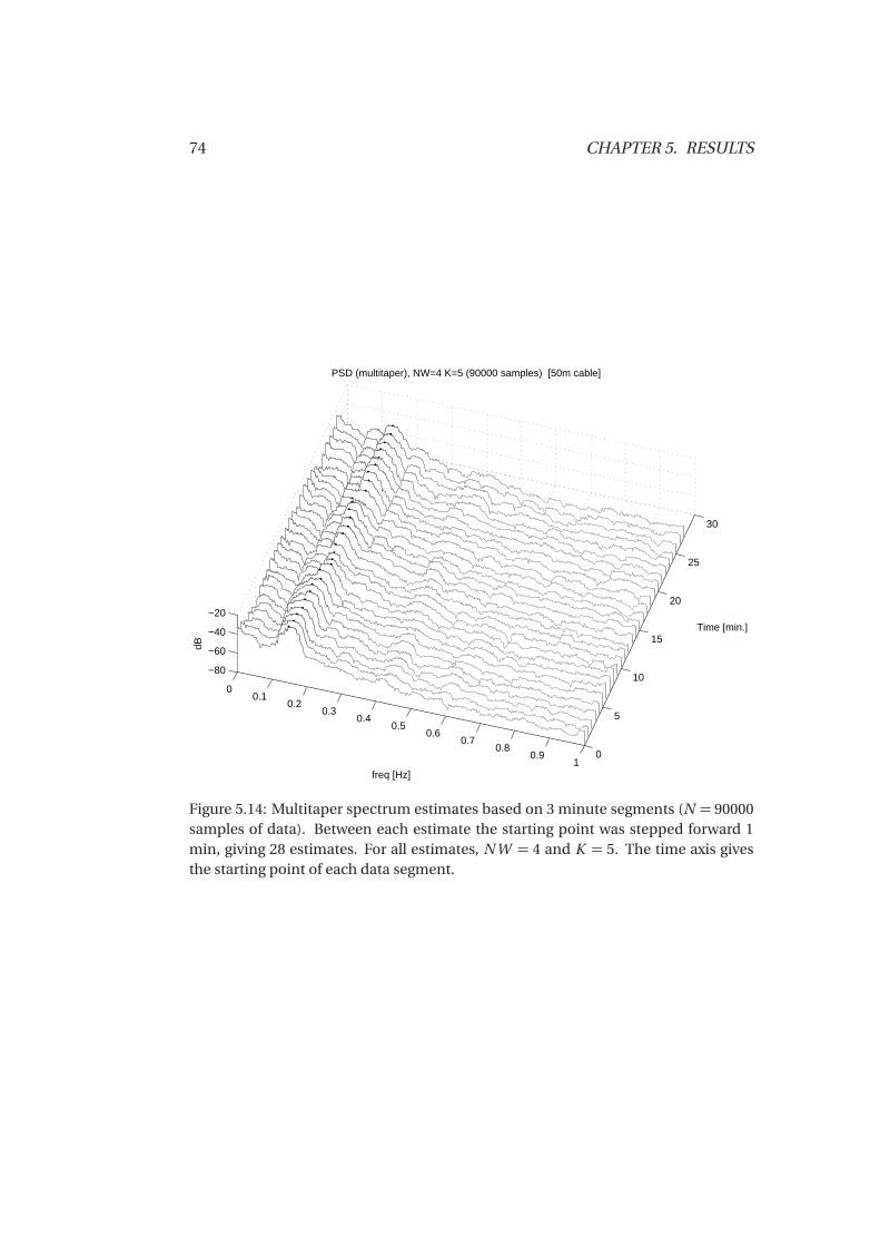
74 CHAPTER 5. RESULTS
00.1
0.20.3
0.40.5
0.60.7
0.80.9
10
5
10
15
20
25
30
−80
−60
−40
−20Time [min.]
PSD (multitaper), NW=4 K=5 (90000 samples) [50m cable]
freq [Hz]
dB
Figure 5.14: Multitaper spectrum estimates based on 3 minute segments (N = 90000samples of data). Between each estimate the starting point was stepped forward 1min, giving 28 estimates. For all estimates, N W = 4 and K = 5. The time axis givesthe starting point of each data segment.

5.1. E-FIELD MEASUREMENTS: 50 M CABLE ANTENNA, STATION 1 75
freq. [Hz]
Tim
e [m
in.]
Contour plot of spectrum estimates, NW = 4, K = 5. Values given by colorbar (dB)
0 0.1 0.2 0.3 0.4 0.5 0.6 0.7 0.8 0.9 10
3
6
9
12
15
18
21
24
27
−85
−80
−75
−70
−65
−60
−55
−50
−45
−40
−35
−30
Figure 5.15: Contour plot of the same estimates as in Figure 5.14, for the frequencyrange 0-1 Hz. The power level in dB is given by the colorbar, and the contour lines arespaced by 10 dB, starting at -30 dB.
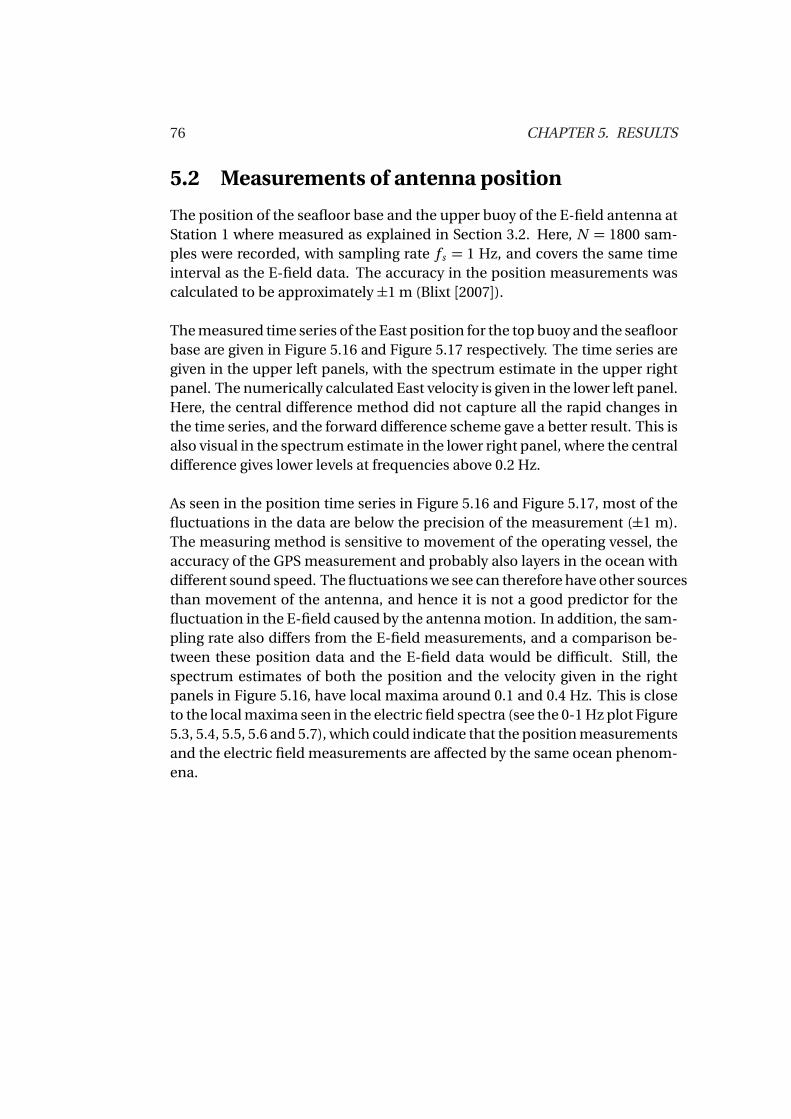
76 CHAPTER 5. RESULTS
5.2 Measurements of antenna position
The position of the seafloor base and the upper buoy of the E-field antenna atStation 1 where measured as explained in Section 3.2. Here, N = 1800 sam-ples were recorded, with sampling rate f s = 1 Hz, and covers the same timeinterval as the E-field data. The accuracy in the position measurements wascalculated to be approximately±1 m (Blixt [2007]).
The measured time series of the East position for the top buoy and the seafloorbase are given in Figure 5.16 and Figure 5.17 respectively. The time series aregiven in the upper left panels, with the spectrum estimate in the upper rightpanel. The numerically calculated East velocity is given in the lower left panel.Here, the central difference method did not capture all the rapid changes inthe time series, and the forward difference scheme gave a better result. This isalso visual in the spectrum estimate in the lower right panel, where the centraldifference gives lower levels at frequencies above 0.2 Hz.
As seen in the position time series in Figure 5.16 and Figure 5.17, most of thefluctuations in the data are below the precision of the measurement (±1 m).The measuring method is sensitive to movement of the operating vessel, theaccuracy of the GPS measurement and probably also layers in the ocean withdifferent sound speed. The fluctuations we see can therefore have other sourcesthan movement of the antenna, and hence it is not a good predictor for thefluctuation in the E-field caused by the antenna motion. In addition, the sam-pling rate also differs from the E-field measurements, and a comparison be-tween these position data and the E-field data would be difficult. Still, thespectrum estimates of both the position and the velocity given in the rightpanels in Figure 5.16, have local maxima around 0.1 and 0.4 Hz. This is closeto the local maxima seen in the electric field spectra (see the 0-1 Hz plot Figure5.3, 5.4, 5.5, 5.6 and 5.7), which could indicate that the position measurementsand the electric field measurements are affected by the same ocean phenom-ena.
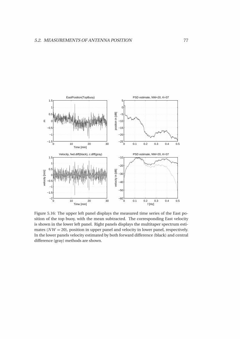
5.2. MEASUREMENTS OF ANTENNA POSITION 77
0 10 20 30−1.5
−1
−0.5
0
0.5
1
1.5EastPosition(TopBuoy)
Time [min]
m
0 0.1 0.2 0.3 0.4 0.5−25
−20
−15
−10
−5
0
5PSD estimate, NW=20, K=37
posi
tion
in [d
B]
0 10 20 30−2
−1.5
−1
−0.5
0
0.5
1
1.5
velo
city
[m/s
]
Time [min]
Velocity, fwd.diff(black), c.diff(gray)
0 0.1 0.2 0.3 0.4 0.5−60
−50
−40
−30
−20
−10
f [Hz]
velo
city
in [d
B]
PSD estimate, NW=20, K=37
Figure 5.16: The upper left panel displays the measured time series of the East po-sition of the top buoy, with the mean subtracted. The corresponding East velocityis shown in the lower left panel. Right panels displays the multitaper spectrum esti-mates (N W = 20), position in upper panel and velocity in lower panel, respectively.In the lower panels velocity estimated by both forward difference (black) and centraldifference (gray) methods are shown.
78 CHAPTER 5. RESULTS
0 10 20 30−2
−1
0
1
2
3EastPosition(Base)
Time [min]
m
0 0.1 0.2 0.3 0.4 0.5−25
−20
−15
−10
−5
0
5PSD estimate, NW=20, K=37
posi
tion
in [d
B]
0 10 20 30−3
−2
−1
0
1
2
3
velo
city
[m/s
]
Time [min]
Velocity, fwd.diff(black), c.diff(gray)
0 0.1 0.2 0.3 0.4 0.5−60
−50
−40
−30
−20
−10
f [Hz]
velo
city
in [d
B]
PSD estimate, NW=20, K=37
Figure 5.17: The upper left panel displays the measured time series of the East posi-tion of the seafloor base, with the mean subtracted. The corresponding East velocityis shown in the lower left panel. Right panels displays the multitaper spectrum esti-mates (N W = 20), position in upper panel and velocity in lower panel, respectively.In the lower panels velocity estimated by both forward difference (black) and centraldifference (gray) methods are shown.
5.3. GEOMAGNETIC ACTIVITY 79
5.3 Geomagnetic activity
To compare the measured vertical electric field with the geomagnetic activ-ity, we got data from the nearest on-land geomagnetic station (Solund, 61°N,4.5°E, Tromsø Geophysical Observatory [2007]). The data from the same timeperiod are shown in Figure 5.18. Here, the figure gives the fluctuation aroundthe sample mean values, and given in the same coordinate system as in Fig-ure 2.2. The respective subtracted mean values were, Fy ≈ 14504 nT (North),Fx ≈−376 nT (positive East) and Fz ≈−48836 nT (Vertical, positive upwards).
The geomagnetic data were sampled every ∆t = 10 s, and this sampling in-terval excludes a direct comparison with the electric field measurement atfrequencies above 0.05 Hz, which is below the range of main interest, namely0.1-10 Hz. If we look at the overall trend in the vertical electric field measure-ments, the mean level changes about 0.11 µV/m during the 30 minutes (seeFigure 5.1 and Table 5.1). The North component of the geomagnetic field, Fy
(upper panel Figure 5.18), is the main contributor to the vertical electric field,and the geomagnetic variation do not match the shape of the trend in the elec-tric field measurements. In addition the geomagnetic variation is small. Byassuming an East directed water velocity of 1 m/s, the fluctuation in the elec-tric field at sea level would be in the same range as the geomagnetic Northfluctuation, i.e., a few nV/m. The fluctuation of the geomagnetic field willthen be attenuated by the ocean, which further reduces its effect on the ver-tical electric field measured at the seafloor. This indicates that the trend seenin the electric field measurements is not caused by the variations of the geo-magnetic field.
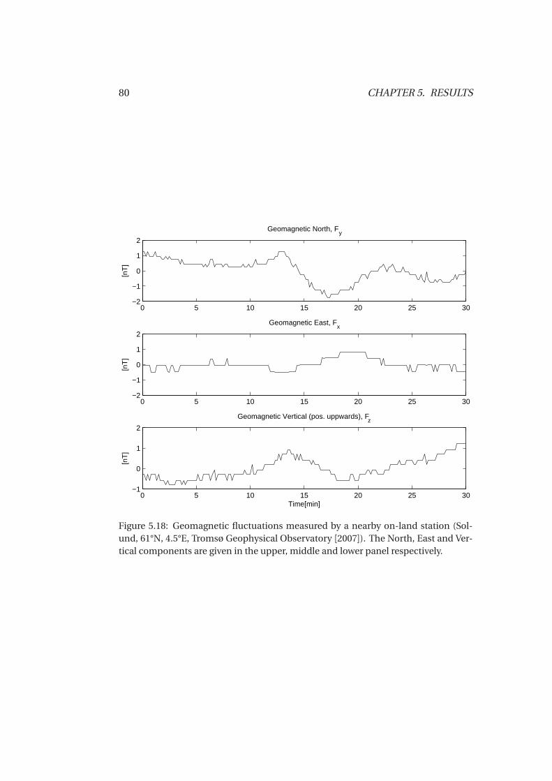
80 CHAPTER 5. RESULTS
0 5 10 15 20 25 30−2
−1
0
1
2
Geomagnetic North, Fy
[nT
]
0 5 10 15 20 25 30−2
−1
0
1
2
Geomagnetic East, Fx
[nT
]
0 5 10 15 20 25 30−1
0
1
2
Geomagnetic Vertical (pos. uppwards), Fz
Time[min]
[nT
]
Figure 5.18: Geomagnetic fluctuations measured by a nearby on-land station (Sol-und, 61°N, 4.5°E, Tromsø Geophysical Observatory [2007]). The North, East and Ver-tical components are given in the upper, middle and lower panel respectively.
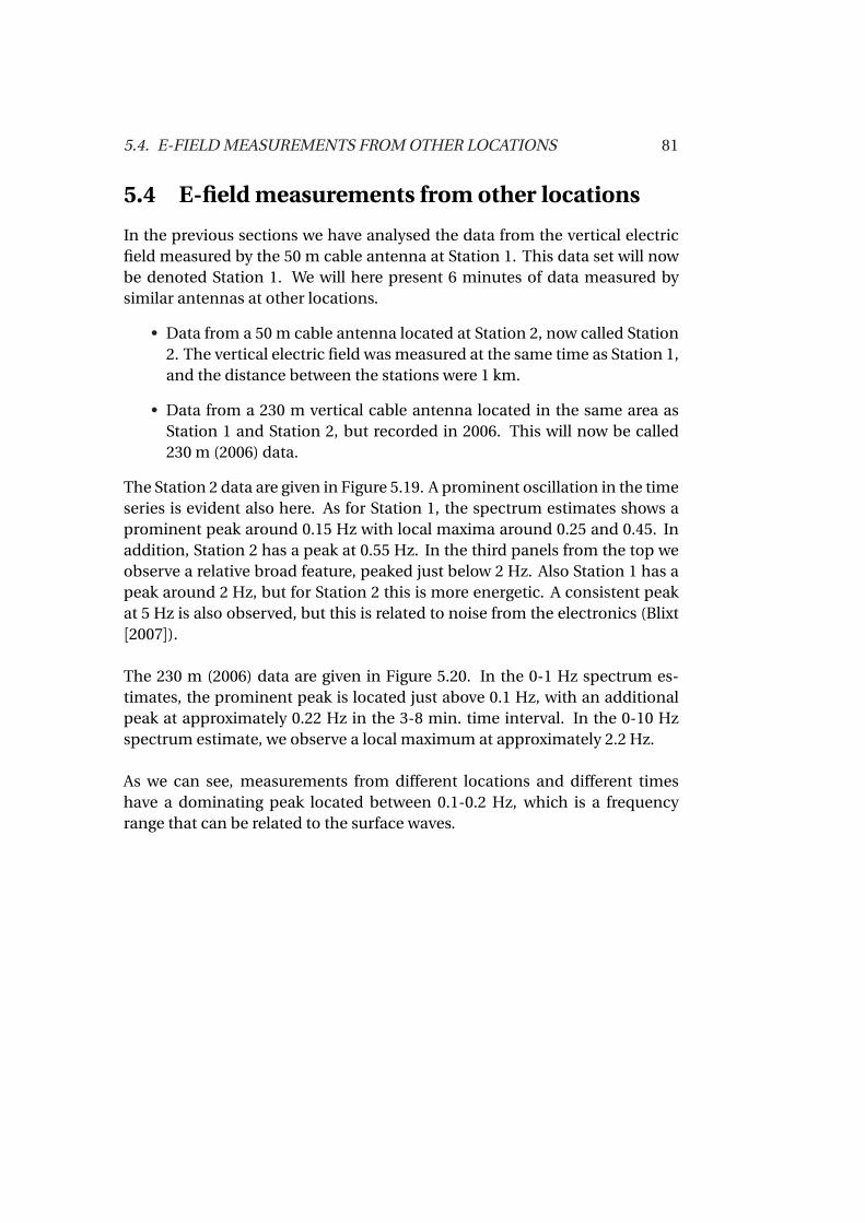
5.4. E-FIELD MEASUREMENTS FROM OTHER LOCATIONS 81
5.4 E-field measurements from other locations
In the previous sections we have analysed the data from the vertical electricfield measured by the 50 m cable antenna at Station 1. This data set will nowbe denoted Station 1. We will here present 6 minutes of data measured bysimilar antennas at other locations.
• Data from a 50 m cable antenna located at Station 2, now called Station2. The vertical electric field was measured at the same time as Station 1,and the distance between the stations were 1 km.
• Data from a 230 m vertical cable antenna located in the same area asStation 1 and Station 2, but recorded in 2006. This will now be called230 m (2006) data.
The Station 2 data are given in Figure 5.19. A prominent oscillation in the timeseries is evident also here. As for Station 1, the spectrum estimates shows aprominent peak around 0.15 Hz with local maxima around 0.25 and 0.45. Inaddition, Station 2 has a peak at 0.55 Hz. In the third panels from the top weobserve a relative broad feature, peaked just below 2 Hz. Also Station 1 has apeak around 2 Hz, but for Station 2 this is more energetic. A consistent peakat 5 Hz is also observed, but this is related to noise from the electronics (Blixt[2007]).
The 230 m (2006) data are given in Figure 5.20. In the 0-1 Hz spectrum es-timates, the prominent peak is located just above 0.1 Hz, with an additionalpeak at approximately 0.22 Hz in the 3-8 min. time interval. In the 0-10 Hzspectrum estimate, we observe a local maximum at approximately 2.2 Hz.
As we can see, measurements from different locations and different timeshave a dominating peak located between 0.1-0.2 Hz, which is a frequencyrange that can be related to the surface waves.
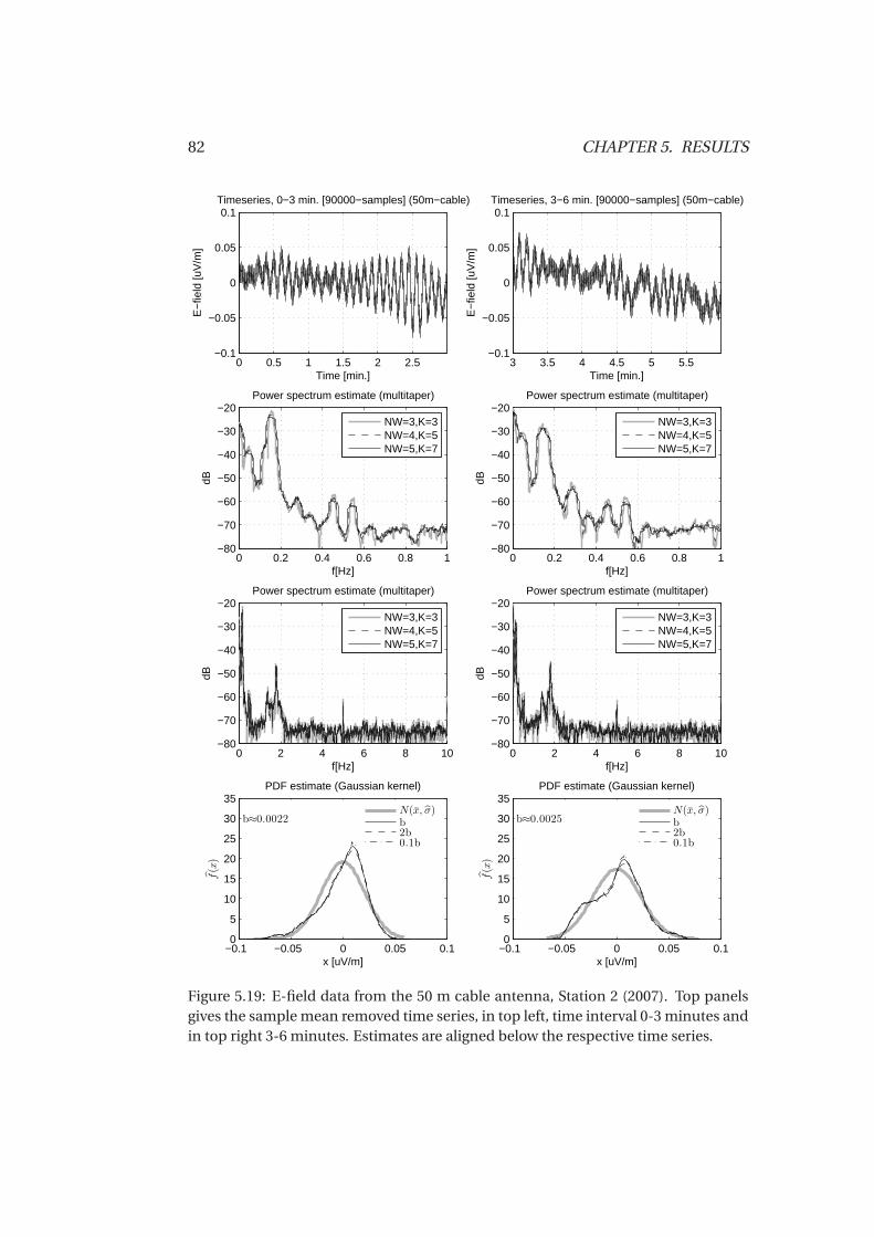
82 CHAPTER 5. RESULTS
0 0.5 1 1.5 2 2.5−0.1
−0.05
0
0.05
0.1
Time [min.]
E−
field
[uV
/m]
Timeseries, 0−3 min. [90000−samples] (50m−cable)
0 0.2 0.4 0.6 0.8 1−80
−70
−60
−50
−40
−30
−20
dB
f[Hz]
Power spectrum estimate (multitaper)
NW=3,K=3NW=4,K=5NW=5,K=7
0 2 4 6 8 10−80
−70
−60
−50
−40
−30
−20
dB
f[Hz]
Power spectrum estimate (multitaper)
NW=3,K=3NW=4,K=5NW=5,K=7
−0.1 −0.05 0 0.05 0.10
5
10
15
20
25
30
35
x [uV/m]
f(x
)
PDF estimate (Gaussian kernel)
b≈0.0022N(x, σ)b2b0.1b
3 3.5 4 4.5 5 5.5−0.1
−0.05
0
0.05
0.1
Time [min.]
E−
field
[uV
/m]
Timeseries, 3−6 min. [90000−samples] (50m−cable)
0 0.2 0.4 0.6 0.8 1−80
−70
−60
−50
−40
−30
−20
dB
f[Hz]
Power spectrum estimate (multitaper)
NW=3,K=3NW=4,K=5NW=5,K=7
0 2 4 6 8 10−80
−70
−60
−50
−40
−30
−20
dB
f[Hz]
Power spectrum estimate (multitaper)
NW=3,K=3NW=4,K=5NW=5,K=7
−0.1 −0.05 0 0.05 0.10
5
10
15
20
25
30
35
x [uV/m]
f(x
)
PDF estimate (Gaussian kernel)
b≈0.0025N(x, σ)b2b0.1b
Figure 5.19: E-field data from the 50 m cable antenna, Station 2 (2007). Top panelsgives the sample mean removed time series, in top left, time interval 0-3 minutes andin top right 3-6 minutes. Estimates are aligned below the respective time series.
5.4. E-FIELD MEASUREMENTS FROM OTHER LOCATIONS 83
0 0.5 1 1.5 2 2.5−2
−1
0
1
2
Time [min.]
E−
field
[uV
/m]
Timeseries, 0−3 min. [90000−samples] (230m−cable)
0 0.2 0.4 0.6 0.8 1−40
−30
−20
−10
0
10
dB
f[Hz]
Power spectrum estimate (multitaper)
0 2 4 6 8 10−60
−50
−40
−30
−20
−10
0
10
dB
f[Hz]
Power spectrum estimate (multitaper)
−3 −2 −1 0 1 20
0.5
1
1.5
x [uV/m]
f(x
)
PDF estimate (Gaussian kernel)
3 3.5 4 4.5 5 5.5−2
−1
0
1
2
Time [min.]E
−fie
ld [u
V/m
]
Timeseries, 3−6 min. [90000−samples] (230m−cable)
0 0.2 0.4 0.6 0.8 1−40
−30
−20
−10
0
10
dB
f[Hz]
Power spectrum estimate (multitaper)
0 2 4 6 8 10−60
−50
−40
−30
−20
−10
0
10
dB
f[Hz]
Power spectrum estimate (multitaper)
−3 −2 −1 0 1 20
0.2
0.4
0.6
0.8
x [uV/m]
f(x
)
PDF estimate (Gaussian kernel)
NW=3,K=3NW=4,K=5NW=5,K=7
NW=3,K=3NW=4,K=5NW=5,K=7
N(x, σ)b2b0.1b
NW=3,K=3NW=4,K=5NW=5,K=7
NW=3,K=3NW=4,K=5NW=5,K=7
N(x, σ)b2b0.1b
Figure 5.20: E-field data from the 230 m cable antenna, recorded in 2006. Top panelsgives the sample mean removed time series, in top left, time interval 0-3 minutes andin top right 3-6 minutes. Estimates are aligned below the respective time series.

Chapter 6
Discussion and conclusions
Data
Electric field data measured by vertical antennas at the seafloor has been anal-ysed in this thesis. Main emphasis is on a data set collected at 20:54 UTC, Sept.19, 2007 at a depth of 316 m below sea surface. Hereafter referenced to as theStation 1 data. Data from the other antennas are named Station 2 and 230 m(2006). If not specified the discussion treat the Station 1 data.
Methods
The spectrum of the vertical electric field has a large dynamic range, includ-ing a rather steep peak up to -20 dB, followed by a rapid fall off to the flatregion below -70 dB, including several sinusoidal components at the higherfrequencies. The data are also dynamic as a function of time, where the am-plitude and the contribution from different frequencies changes during time.Hence, this is rather complicated data to resolve. The multitaper methodwe implemented, can be applied to relatively short time segments, and bya proper selection of the number of averaged eigenspectra, still provide goodbias and variance properties and a reasonable frequency resolution. In ad-dition, we can easily apply several independent estimates, by adjusting thefrequency resolution parameter N W . Then, by comparing the different esti-mates, consistent features seen in several spectral estimates can be revealedand strengthen their status as true features in the spectrum.
By the use of the multitaper method, we can also extend the analysis withan F -test to evaluate the significance of possible present sinusoidal compo-nents. A slowly varying background spectrum, which is the basis of this test, isnot fulfilled for our data at the low frequencies (below 1 Hz). Hence, this canexplain the low F -values at the prominent peaks between 0.1-0.3 Hz in most
85
86 CHAPTER 6. DISCUSSION AND CONCLUSIONS
of our tests. In addition, we also encounter problems if the amplitude andphase of the periodic components vary, or if several sinusoidals are presentwith a spacing less than the half-bandwidth W . Therefore, the comparison ofdifferent spectral estimates seems to be the most powerful way to reveal truepeaks and features at the low frequencies. Still, the F -test provides valuableinformation, and in particularly for the higher frequencies (where the spec-trum becomes more flat) and it can be used to search for unphysical compo-nents generated by the electronics. As we made an automatic F -test routine,the test can easily be applied to many data sets, or to the same data but withdifferent parameters. By using both the comparison between several multita-per estimates, and the F -test, the spectrum analysis becomes more complete.We used the multitaper method based on the arithmetic average of severaleigenspectra, and the three highest order potentially usable DPSS tapers wereexcluded in our analysis.
For estimation of the probability density function we used the standard non-parametric kernel methods. The kernel width was chosen according to Silver-man’s rule-of-thumb. The kernel estimators produce a smooth, continuousand differentiable function estimate, which is preferred for further analysisand calculations based on the estimate. To further reveal consistency in theestimates we could have used even more fixed kernel widths, or alternativelywe could have used the adaptive method to select the kernel width (e.g., Sil-verman [1986]). The electric field data were found to be non-Gaussian, indi-cated both by the kernel estimates and the sample moments. If we excludethe time intervals flagged as nonstationary by the runs test, the data were leftskewed, and with lighter tails than Gaussian distributions.
The implemented runs test is a rather simplistic indicator for trends and lackof stationarity in a data set. Still, it has proven to be useful when we evaluateour estimates.
Observations
The maximum peak in the electric field spectrum is around 0.15 Hz. It variesslightly in frequency, but the level changes more than 10 dB during the 30 min-utes of recordings. The frequency of the maximum peak corresponds closelyto the frequency of the mean frequency of the surface waves. In addition,the shoulder just above 0.1 Hz, indicating a secondary peak, corresponds tothe frequency of the maximum surface waves (0.12 Hz). The peak seen at0.24 Hz, then correspond to the double frequency of the maximum surfacewaves. Hence, we see an obvious relation between the measured electric field
87
and the sea surface waves. Also the data from Station 2 have a prominentpeak around 0.15 Hz, which supports this relation. While the prominent peakis located around 0.1-0.2 Hz for both Station 1, Station 2 and the 230 m (2006)data, we also note the differences in the spectrum at frequencies above 0.2 Hz.Particularly, the feature seen at around 2 Hz for all the antennas, has a sub-stantially different shape and level for data recorded by the different anten-nas, indicating a common origin but with local variations.
In general the amplitude of the electric field fluctuations were less than0.07 µV/m (Station 1). If we assume that the antenna was completely station-ary during the recordings, we can relate this to an average fluctuation in thewater between the electrodes (horizontal, East-West). By using the measurednorth component of the magnetic field of Fy = 14504 nT, this indicates a fluc-tuating water velocity with amplitude less than 5 mm/s. If the cable and theupper electrode of the antenna were moving, it would likely be with a velocityin the same range as the fluctuating water. Hence, the accuracy (±1 m) offeredby the position data from the experiment is not accurate enough to determinethe small scale movement of the antenna.
The electrodes were located at depths of 316 m (seafloor) and 266 m respec-tively and the 2D linear wave theory can not explain the horizontal velocitiesin the mm/s range at these depths for a single surface wave with period 6.8 s.E.g., for a surface wave described as a single periodic wave train, the elevationof the surface causes circular particle motion below the surface. For a finitedepth d , the wave number k is given through the linear dispersion relation(e.g., Sarpkaya and Isaacson [1981](p.155))
ω2 = g k tanh(k d ), (6.1)
were g = 9.81 m/s2. The amplitude of the horizontal velocity beneath thesurface is given by (e.g., Sarpkaya and Isaacson [1981](p.157))
v (z ) =πH
T
cosh(k z +k d )sinh(k d )
. (6.2)
Here, z = 0 at the flat surface, and z = −d at the seafloor and H is the totalwave height of the surface wave (twice the amplitude from the flat surface).By solving Eq. (6.1) numerically for the observed mean surface wave periodT = 6.8 s (ω= 2π/T ), we obtain the wave number k = 0.08703 m−1. If we thensolve Eq. (6.2) for this wave number, and a finite depth of d = 316 m and awave height H = 4 m, the amplitude of the horizontal particle velocity at theupper electrode z = −266 m, will be in the range 10−7 mm/s and will be fur-ther reduced close to the seafloor. Hence, this is far from the velocity 5 mm/s
88 CHAPTER 6. DISCUSSION AND CONCLUSIONS
indicated by the electric field fluctuation, and a linear model of the subsur-face water motion due to the surface waves do not explain the results.
No obvious correspondence was observed between the geomagnetic field andthe measured electric field. The trend seen in the vertical electric field time se-ries could be caused by a drift in the DC-level of the electrodes. Quite possibleit could also be caused by changes in the mean water velocity, e.g., because oftidal movements of the sea water.
Most likely, the fluctuations we see in the electric field is caused by interac-tion between surface waves. Theory (e.g., Longuet-Higgins [1950] and Kibble-white and Wu [1991]) shows that the nonlinear interaction between surfacewaves generates pressure fluctuation which can propagate through the oceanand reach the seafloor even at great depths. The pressure fluctuation causeboth water and seafloor motion, and can hence induce electric field fluctu-ations (Cox et al. [1978], Webb and Cox [1986]). In the latter papers promi-nent oscillation were measured in the horizontal electric field at the seafloor,with spectra having peaks between 0.1-0.2 Hz, and through theory related tothe pressure fluctuation and seafloor motion. The disturbance of the seaflooris called microseism, and is evident between 0.1-5 Hz in both displacementand pressure spectra at the seafloor, with a typically peak between 0.1-0.2 Hz(Webb [1992]).
For a vertical antenna the "local" source of the measured electric field is rathercomplex to determine, as the pressure fluctuation can produce movementboth in the water and the seafloor. As one end of the antenna is fixed to theseafloor and the other end is held up by a buoy, the measured electric fieldwill be caused by a combination of the water, antenna and seafloor motion.The spectrum estimates of the electric field presented here, shows that theprominent peak are present in the range 0.1 Hz to 0.2 Hz for three differentantennas, measured at different times and locations. As prominent peaks inthe spectrum between 0.1-0.3 Hz seems to be present in all measurement ofthe electric field at the seafloor (Cox et al. [1978], Webb and Cox [1986], Chaveet al. [1991]), and is also present in displacement and pressure spectra, it is notexpected that the signal can be removed by e.g., redesigning the antennas. Aslong as the frequencies around 0.1-0.3 Hz is of interest for CSEM, this motioninduced signal needs to be carefully monitored and analysed in order for it tobe removed from the desired CSEM signal.

Bibliography
J. S. Bendat and A. G. Piersol. Random Data: Analysis and Measurement Procedures.Wiley-Interscience, 3 edition, 2000.
N. Bindoff, J.H.Filloux, P. Mulhearn, F. Lilley, and I. Ferguson. Vertical electric fieldfluctuations at the floor of the tasman abyssal plain. Deep-Sea Research, 33(5):587–600, 1986.
M. Blixt, 2007. Personal communication.
T. Bronez. On the performance advantage of multitaper spectral analysis. IEEE Trans-actions on Signal Processing, 40(12):2941–2946, Dec 1992.
A. Chave and J. Filloux. Observation and interpretation of the seafloor vertical elec-tric field in the eastern north pacific. Geophysical Research Letters, 12(12):793–796,1985.
A. Chave, S. Constable, and N. Edwards. Electrical exploration methods for theseafloor. In Electromagnetic methods in applied geophysics-Applications, chap-ter 12, pages 931–966. Society of Exploration Geophysicists, 1991.
A. D. Chave. On the electromagnetic fields induced by oceanic internal waves. Geo-physical research, 89(C6):10,519–10,528, Nov. 1984.
A. D. Chave, J. H. Filloux, and D. S. Luther. Electromagnetic induction by ocean cur-rents: Bempex. Physics of the Earth and Planetary Interiors, 53(3-4):350–359, 1989.
S. Constable and L. Srnka. An introduction to marine controlled-source electromag-netic methods for hydrocarbon exploration. Geophysics, 72(2):WA3–WA12, 2007.
C. Cox, N. Kroll, P. Pistek, and K. Watson. Electromagnetic fluctation induced bywind waves on the deep-sea floor. Journal of Geophysical Research, 83(C1):431–442, 1978.
M. B. Dobrin and C. H. Savit. Introduction to Geophysical Prospecting. McGraw-HillBook Company, 1988.
89
90 BIBLIOGRAPHY
A. Eberhard. An optimal discrete window for the calculation of power spectra. IEEETransactions on Audio and Electroacoustics, AU-21(1), Feb 1973.
T. Eidesmo, S. Ellingsrud, L. MacGregor2, S. Constable, M. Sinha, S. Johansen, F. Kong,and H. Westerdahl. Sea bed logging (sbl), a new method for remote and directidentification of hydrocarbon filled layers in deepwater areas. first break, 20(3):144–152, 2002.
S. Ellingsrud, T. Eidsmo, S. Johansen, M. C. Sinha, L. MacGregor, and S. Constable. Re-mote sensing of hydrocarbon layers by seabed logging (sbl): Results from a cruiseoffshore angola. The Leading Edge, (21):972–982, 2002.
J. Filloux. Techniques and instrumentation for study of natural electromagnetic in-duction at sea. Physics of the Earth and Planetary Interiors, 7:323–338, 1973.
A. Hanssen. Introduction to statistical signal processing and data analysis. PhysicsDepartment, University of Tromsø, 2003. Lecture Notes Fys-261.
A. Hanssen, J. Kongsli, R. Hansen, and S. Chapman. Statistics of synthetic aperturesonar images. Proceedings of OCEANS 2003, 5:2635 – 2640, 22-26 Sept. 2003. SanDiego, CA.
F. J. Harris. On the use of windows for harmonic analysis with the discrete fouriertransform. Proceedings of the IEEE, 66(1), 1978.
R. R. Harvey and J. C. L. R. Montaner. Electric field recording of tidal currents in thestrait of magellan. Geophysical research, 82(24):3472–3476, Aug. 1977.
http://www.km.kongsberg.com. Mst mini ssbl transponders instruction man-ual. http://www.km.kongsberg.com/KS/WEB/NOKBG0240.nsf/AllWeb\\/5C49119DBC28AF52C1256EF6004185CB?OpenDocument, 8.Nov 2007.
S. E. Johansen, H. E. F. Amundsen, T. Røsten, T. E. S. Ellingsrud, and A. H. Bhuyian.Subsurface hydrocarbons detected by electromagnetic sounding. First Break, (23):31– 36, 2005.
J. Kaiser and R. Schafer. On the use of the lo-sinh window for spectrum analysis. IEEETransactions on acoustics, speech, and signal processing, ASSP-28(1), 1980.
G. K. Keller. Rock and mineral properties. In M. N. Nabighian, editor, Electromagneticmethods in applied geophysics – Theory. Vol. 1, pages 12–51. Society of ExplorationGeophysicists, 1987.
A. C. Kibblewhite and C. Y. Wu. The theoretical description of wave-wave interactionsas a noise source in the ocean . Acoustical Society of America Journal, 89:2241–2252,May 1991.

91
F. N. Kong, H. Westerdahl, S. Ellingsrud, T. Eidesmo, and J. Johansen. ’seabed logging’:A possible direct hydrocarbon indicator for deepsea prospects using em energy. Oiland Gas Journal, (100):30–38, 2002.
R. H. Landau and M. J. Pàez. Computational Physics. Wiley-vch, 2004.
J. Larsen. An introduction to electromagnetic induction in the ocean. Physics of theEarth and Planetary Interiors, 7:389–398, 1973.
J. Larsen. Transport and heat flux of the florida current at 27°n derived from cross-stream voltage and profiling data: theory and observations. Philosophical Trans-action: Physical Science and Engineering, 338:169–236, 1992.
J. Lees and J. Park. Multiple-taper spectral analysis: A stand-alone c-subroutine.Computer and Geosciences, 21(2):199–236, 1995.
J. M. Lees. Reshaping spectrum estimates by removing periodic noise: Application toseismic spectral ratios. Geophysical research letters, 22(4):513–516, February 1995.
F. Lilley, A. Hitchman, P. Milligan, and T. Pedersen. Sea-surface observations of themagnetic signal of ocean swell. Geophysical Journal International, 159(2):565–572,2004.
M. Longuet-Higgins. A theory of the origin of microseisms. Philosophical Transac-tions of the Royal Society of London. Series A, Mathematical and Physical Sciences,243(857):1–35, 1950.
L. O. Løseth, H. M. Pedersen, B. Ursin, L. Amundsen, and S. Ellingsrud. Low-frequency electromagnetic fields in applied geophysics: Waves or diffusion? Geo-physics, 71(4):W29–W40, 2006.
L. MacGregor and S. Sinha. Use of marine controlled-source electromagnetic sound-ing for sub-basalt exploration. Geophysics Prosp., (48):1091–1106, 2000.
M. E. Mann and J. M. Lees. Robust estimation of background noise and signal detec-tion in climatic time series. Climatic Change, 33(3):409–445, July 1996.
Meteorologisk institutt. http://www.met.no, 2007. Weather data from Troll A re-ceived on enquiry.
A. H. Nuttall. Some windows with very good sidelobe behavior. IEEE Transactions onacoustics, speech, and signal processing, ASSP-29(1), 1981.
N. Palshin, L. Vanyan, A. Poray-Kohits, V. Matyushenko, P. Kaikkonen, and J. Ti-ikkainen. Measurements of motionally induced voltage in the coastal zone of thethroat of the white sea. Earth Planets Space, 54:433–441, 2002.

92 BIBLIOGRAPHY
N. Palshin, A. Nozdrina, V. Matyushenko, A. Porai-Koshits, and I. V. Egorov. Electro-magnetic method for monitoring currents in the gorlo of the white sea. Oceanol-ogy, 46(3):325–334, 2006.
E. Parzen. On estimation of a probability density function and mode. The Annals ofMathematical Statistics, 33(3):1065–1076, Sep 1962.
D. B. Percival and A. T. Walden. Spectral analysis for physical applications: Multitaperand Conventional Univariate Techniques. Cambridge University Press, 1993.
W. H. Press, S. A.Teukolsky, W. T. Vetterling, and B. P. Flannery. Numerical recipes inC: the art of scientific computing. Cambridge university press, 2nd edition, 1992.ISBN 0-521-43108-5.
K. S. Riedel and A. Sidorenko. Minimum bias multiple taper spectral estimation. IEEETransactions on signal processing, 43(1), Jan. 1995.
T. B. Sanford. Motionally induced electric and magnetic fields in the sea. Journal ofGeophysical Research, 76, 1971.
T. Sarpkaya and M. Isaacson. Mechanics of wave forces on offshore structures, chapter4. Wave theories. Van Nostrand Reinhold Co., New York, 1981. ISBN 0442254024.
R. Shiavi. Introduction to Applied Statistical Signal Analysis. Academic Press, 2 edi-tion, 1999.
B. Silverman. Density estimation for statistics and data analysis. Chapman and Hall,first edition, 1986.
D. Slepian. Some comments on fourier analysis, uncertainty and modeling. Societyfor Industrial and Applied Mathematics, 25(3):379–393, July 1983.
D. Slepian. Prolate spheroidal wave functions, fourier analysis, and uncertainty. v -the discrete case. Bell System Technical Journal, 57:1371–1430, 1978.
H. Stark and J. W. Woods. Probability and Random Processes with Applications toSignal Processing. Prentice-Hall, 3 edition, 2002.
A. Stuart and J. K. Ord. Kendall’s advanced theory of statistics, volume 1. CharlesGriffin & Co., London, fifth edition, 1987. Originally by Sir Maurice Kendall.
G. Sutton and N. Barstow. Ocean-bottom ultralow-frequency (ulf) seismo-acousticambient noise: 0.002 to 0.4 hz. The Journal of the Acoustical Society of America, 87(5):2005–2012, 1990.
S. Theodoridis and K. Koutroumbas. Pattern recognition. Academic Press, 1998. ISBN0-12-686140-4.

93
D. J. Thomson. Spectrum estimation and harmonic analysis. Proceedings of the IEEE,70(9):1055–1096, September 1982.
Tromsø Geophysical Observatory. Geomagnetic data. http://geo.phys.uit.no/geomag.html, Oct 2007. Faculty of Science University of Tromsø, Norway.
M. Wand and M. Jones. Kernel Smoothing. Chapman and Hall/CRC, 1 edition, 1995.ISBN 0-412-55270-1.
S. Webb and C. Cox. Observations and modeling of seafloor microseisms. Journal ofGeophysical Research, 91(B7):7343–7358, 1986.
S. C. Webb. The equilibrium oceanic microseism spectrum . Acoustical Society ofAmerica Journal, 92:2141–2158, Oct. 1992.
P. D. Welch. The use of fast fourier transform for the estimation of power spectra: Amethod based on time averaging over short, modified periodograms. IEEE trans-actions on audio and electroacoustics, AU-15(2):70–73, 1967.
Related Documents


![moDel legislation For electromagnetic FielDs protection1].pdf · moDel legislation For electromagnetic FielDs protection. ... Model legislation for electromagnetic fields ... If a](https://static.cupdf.com/doc/110x72/5b166fc57f8b9a4a6d8befdf/model-legislation-for-electromagnetic-fields-1pdf-model-legislation-for-electromagnetic.jpg)
