Mosquito Image Classification using Convolutional Neural ...

Louisiana State UniversityLSU Digital Commons

LSU Master's Theses Graduate School

March 2019

Mosquito Image Classification usingConvolutional Neural NetworksSumanth VissamsettyLouisiana State University and Agricultural and Mechanical College, [email protected]

Follow this and additional works at: https://digitalcommons.lsu.edu/gradschool_theses

Part of the Computer Sciences Commons, and the Entomology Commons

This Thesis is brought to you for free and open access by the Graduate School at LSU Digital Commons. It has been accepted for inclusion in LSUMaster's Theses by an authorized graduate school editor of LSU Digital Commons. For more information, please contact [email protected].

Recommended CitationVissamsetty, Sumanth, "Mosquito Image Classification using Convolutional Neural Networks" (2019). LSU Master's Theses. 4889.https://digitalcommons.lsu.edu/gradschool_theses/4889

MOSQUITO IMAGE CLASSIFICATION USING CONVOLUTIONAL NEURALNETWORKS

A Thesis

Submitted to the Graduate Faculty of theLouisiana State University and

Agricultural and Mechanical Collegein partial fulfillment of the

requirements for the degree ofMaster of Science

in

Department of Computer Science

bySumanth Vissamsetty

B.Tech, GITAM University, 2016May 2019

Acknowledgments

Firstly, I would like to thank my family for all the love, care, support and sacrifices

they have made for my successful academic career.

I would like to thank Dr. Jianhua Chen for being a very understanding and supportive

advisor. Even though we redefined our research problem I am glad that we ended up finding

a good problem and doing good research to achieve likewise results.

Also, a very special thanks to Dr. Athanasios Gentimis for constantly motivating me.

His intriguing insights for various concepts and problems not only helped me understand

and solve the problem, it also strengthened my knowledge base.

I would also show my gratitude to Dr. Konstantin Busch for taking time out of his

busy schedule and being a core committee member of masters’ thesis.

I thank all my friends for making my stay pleasant, happy and stress-free in this foreign

land.

Last but not least I thank St. Tammany Parish Mosquito Abatement Center for col-

laborating on this research project with us.

ii

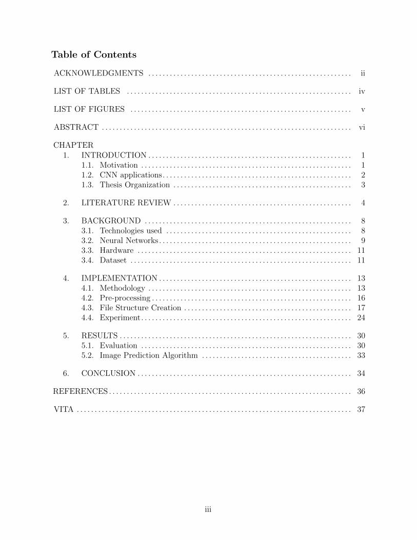
Table of Contents

ACKNOWLEDGMENTS . . . . . . . . . . . . . . . . . . . . . . . . . . . . . . . . . . . . . . . . . . . . . . . . . . . . . . . . . ii

LIST OF TABLES . . . . . . . . . . . . . . . . . . . . . . . . . . . . . . . . . . . . . . . . . . . . . . . . . . . . . . . . . . . . . . . iv

LIST OF FIGURES . . . . . . . . . . . . . . . . . . . . . . . . . . . . . . . . . . . . . . . . . . . . . . . . . . . . . . . . . . . . . . v

ABSTRACT . . . . . . . . . . . . . . . . . . . . . . . . . . . . . . . . . . . . . . . . . . . . . . . . . . . . . . . . . . . . . . . . . . . . . . vi

CHAPTER1. INTRODUCTION . . . . . . . . . . . . . . . . . . . . . . . . . . . . . . . . . . . . . . . . . . . . . . . . . . . . . . . . . 1

1.1. Motivation . . . . . . . . . . . . . . . . . . . . . . . . . . . . . . . . . . . . . . . . . . . . . . . . . . . . . . . . . . . 11.2. CNN applications. . . . . . . . . . . . . . . . . . . . . . . . . . . . . . . . . . . . . . . . . . . . . . . . . . . . . 21.3. Thesis Organization . . . . . . . . . . . . . . . . . . . . . . . . . . . . . . . . . . . . . . . . . . . . . . . . . . 3

2. LITERATURE REVIEW . . . . . . . . . . . . . . . . . . . . . . . . . . . . . . . . . . . . . . . . . . . . . . . . . . 4

3. BACKGROUND . . . . . . . . . . . . . . . . . . . . . . . . . . . . . . . . . . . . . . . . . . . . . . . . . . . . . . . . . . 83.1. Technologies used . . . . . . . . . . . . . . . . . . . . . . . . . . . . . . . . . . . . . . . . . . . . . . . . . . . . 83.2. Neural Networks . . . . . . . . . . . . . . . . . . . . . . . . . . . . . . . . . . . . . . . . . . . . . . . . . . . . . . 93.3. Hardware . . . . . . . . . . . . . . . . . . . . . . . . . . . . . . . . . . . . . . . . . . . . . . . . . . . . . . . . . . . . 113.4. Dataset . . . . . . . . . . . . . . . . . . . . . . . . . . . . . . . . . . . . . . . . . . . . . . . . . . . . . . . . . . . . . . 11

4. IMPLEMENTATION . . . . . . . . . . . . . . . . . . . . . . . . . . . . . . . . . . . . . . . . . . . . . . . . . . . . . . 134.1. Methodology . . . . . . . . . . . . . . . . . . . . . . . . . . . . . . . . . . . . . . . . . . . . . . . . . . . . . . . . . 134.2. Pre-processing . . . . . . . . . . . . . . . . . . . . . . . . . . . . . . . . . . . . . . . . . . . . . . . . . . . . . . . . 164.3. File Structure Creation . . . . . . . . . . . . . . . . . . . . . . . . . . . . . . . . . . . . . . . . . . . . . . . 174.4. Experiment. . . . . . . . . . . . . . . . . . . . . . . . . . . . . . . . . . . . . . . . . . . . . . . . . . . . . . . . . . . 24

5. RESULTS . . . . . . . . . . . . . . . . . . . . . . . . . . . . . . . . . . . . . . . . . . . . . . . . . . . . . . . . . . . . . . . . . 305.1. Evaluation . . . . . . . . . . . . . . . . . . . . . . . . . . . . . . . . . . . . . . . . . . . . . . . . . . . . . . . . . . . 305.2. Image Prediction Algorithm . . . . . . . . . . . . . . . . . . . . . . . . . . . . . . . . . . . . . . . . . . 33

6. CONCLUSION . . . . . . . . . . . . . . . . . . . . . . . . . . . . . . . . . . . . . . . . . . . . . . . . . . . . . . . . . . . . 34

REFERENCES . . . . . . . . . . . . . . . . . . . . . . . . . . . . . . . . . . . . . . . . . . . . . . . . . . . . . . . . . . . . . . . . . . . . 36

VITA . . . . . . . . . . . . . . . . . . . . . . . . . . . . . . . . . . . . . . . . . . . . . . . . . . . . . . . . . . . . . . . . . . . . . . . . . . . . . 37

iii

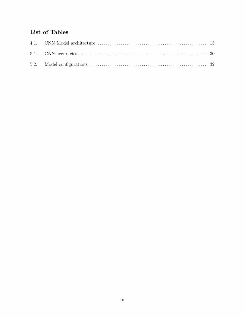
List of Tables

4.1. CNN Model architecture . . . . . . . . . . . . . . . . . . . . . . . . . . . . . . . . . . . . . . . . . . . . . . . . . . . . 15

5.1. CNN accuracies . . . . . . . . . . . . . . . . . . . . . . . . . . . . . . . . . . . . . . . . . . . . . . . . . . . . . . . . . . . . . 30

5.2. Model configurations . . . . . . . . . . . . . . . . . . . . . . . . . . . . . . . . . . . . . . . . . . . . . . . . . . . . . . . . 32

iv

List of Figures

1.1. Mosquito life cycle . . . . . . . . . . . . . . . . . . . . . . . . . . . . . . . . . . . . . . . . . . . . . . . . . . . . . . . . . . 2

3.1. Typical CNN architecture . . . . . . . . . . . . . . . . . . . . . . . . . . . . . . . . . . . . . . . . . . . . . . . . . . . 10

3.2. Sample image of Pupae . . . . . . . . . . . . . . . . . . . . . . . . . . . . . . . . . . . . . . . . . . . . . . . . . . . . . . 12

3.3. Sample image of Instar . . . . . . . . . . . . . . . . . . . . . . . . . . . . . . . . . . . . . . . . . . . . . . . . . . . . . . 12

4.1. Workflow diagram . . . . . . . . . . . . . . . . . . . . . . . . . . . . . . . . . . . . . . . . . . . . . . . . . . . . . . . . . . . 14

4.2. Pre-processed Images . . . . . . . . . . . . . . . . . . . . . . . . . . . . . . . . . . . . . . . . . . . . . . . . . . . . . . . . 164.3. Request for input directory . . . . . . . . . . . . . . . . . . . . . . . . . . . . . . . . . . . . . . . . . . . . . . . . . . 18

4.4. Request for directory to save data . . . . . . . . . . . . . . . . . . . . . . . . . . . . . . . . . . . . . . . . . . . 19

4.5. Request for input ‘data’ directory . . . . . . . . . . . . . . . . . . . . . . . . . . . . . . . . . . . . . . . . . . . . 25

4.6. Model summary . . . . . . . . . . . . . . . . . . . . . . . . . . . . . . . . . . . . . . . . . . . . . . . . . . . . . . . . . . . . . 29

5.1. Accuracies for various configurations . . . . . . . . . . . . . . . . . . . . . . . . . . . . . . . . . . . . . . . . . 31

5.2. Overfitting . . . . . . . . . . . . . . . . . . . . . . . . . . . . . . . . . . . . . . . . . . . . . . . . . . . . . . . . . . . . . . . . . . 32

v

Abstract

Human life has always been affected by insects, especially mosquitoes, since it’s early

beginnings. This pesky insect acts as a vector that transmit pathogens through feeding

on our blood, spreading life-threatening diseases like Zika Virus, Malaria, Dengue fever,

Chikungunya and more. It is important to prevent these mosquitoes from harming humans

and one way to do so is to control the mosquito population, or mosquito abatement as it is

commonly known. It is important to note that not all mosquitoes are the same and each

of them live, reproduce and attack in their own unique way. Hence it is crucial for humans

to identify each of the mosquito species and study them in a detailed manner which turns

out to be a very complicated and time-consuming problem that needs to be solved prior to

any attempt at mosquito control. This gives rise to the need of novel algorithms to identify

mosquitoes through image processing tasks, coupled with automated machine learning

classification techniques. In our thesis, we have used Convolutional Neural Networks to

build an image classification model to identify two life-stages of a mosquito, namely, Instar

4 and Pupae. Our algorithm yielded an average accuracy of over 95%, reducing the time

to process similar classifications by hand to at least a hundredfold.

vi

Chapter 1.Introduction

1.1. Motivation

During the Summer of 2018, the LSU AgCenter got into an agreement with the St.

Tammany Parish Mosquito Abatement, to assist them with their classification and detec-

tion of mosquito development in their lab. The main task of this effort is to generate an

automated, machine learning based method to explore images of mosquitoes in a lab envi-

ronment and potentially the field. The ultimate goal would be an algorithm which reads

an image captured by the staff of the STPMAD and outputs an estimate of the types and

number of mosquitoes present. The program should allow for inherent noise in the image

and it should be robust with respect to lighting conditions and aspect like focus, orientation

depth etc. The final solution reduces the experts’ time spent for the classification task from

several hours to just a couple of seconds.

According to the experts at (STPMAD) there are about 47 different species of

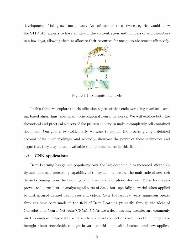
mosquitoes in the general Louisiana area. In this thesis we deal with one particular

mosquito species and follow it during its life cycle. That cycle includes four stages: (a)

Eggs, (b) Larvae/instar, (c) Pupae and (d) Adult mosquito, as described in figure 1.1. The

life cycle of the specific species of mosquito used in this research is a more detailed break-

down of the cycle described above. The first stage is the same i.e., eggs, which are layed by

the adult mosquitoes. The eggs then hatch into 1st instar larvae, which are the smallest,

least developed stage in the mosquito lifecycle. After a few days, 1st instars molt into 2nd

instar larvae, shedding their old husk. This process happens again, producing a larger 3rd

instar larva, and for one last time, producing a large 4th instar larva. 4th instar larvae

molt into pupae, similar to a cocoon, prior to emerging as a fully grown adult mosquito.

Husks are left behind between every instar, and are most obvious as pupae emerge into

the adult stage. In this research we limit our classification to binary, the two classes being

Instar4 (fouth stage instars) and Pupae, since these are the stages directly prior to the

1

development of full grown mosquitoes. An estimate on these two categories would allow

the STPMAD experts to have an idea of the concentration and numbers of adult numbers

in a few days, allowing them to allocate their resources for mosquito abatement effectively.

Figure 1.1. Mosquito life cycle

In this thesis we explore the classification aspect of that endeavor using machine learn-

ing based algorithms, specifically convolutional neural networks. We will explore both the

theoretical and practical aspects of the process and try to make a completely self-contained

document. Our goal is two-fold; firstly, we want to explain the process giving a detailed

account of its inner workings, and secondly, showcase the power of these techniques and

argue that they may be an invaluable tool for researchers in this field.

1.2. CNN applications

Deep Learning has gained popularity over the last decade due to increased affordabil-

ity and increased processing capability of the system, as well as the multitude of new rich

datasets coming from the booming of internet and cell phone devices. These techniques

proved to be excellent at analyzing all sorts of data, but especially powerful when applied

to unstructured dataset like images and videos. Over the last few years, numerous break-

throughs have been made in the field of Deep Learning primarily through the ideas of

Convolutional Neural Networks(CNNs). CNNs are a deep learning architecture commonly

used to analyze image data, or data where spatial connections are important. They have

brought about remarkable changes in various field like health, business and new applica-

2

tions are constantly being discovered in other areas like transportation, agriculture and

others. Some of the CNN’s applications are face recognition, video captioning, image clas-

sification, activity recognition, hand writing recognition, etc. Our thesis can be categorized

under image classification using CNNs.

CNNs, and more generally Deep Learning techniques, that have become popular re-

placements to traditional supervised learning algorithms and advanced statistical tech-

niques due to their ability to work with large datasets (to the order of terabytes). Also it

can be argued that the most challenging areas of traditional tools, like feature extraction,

can be eliminated as the CNNs themselves capture the patterns/features from the training

data.

1.3. Thesis Organization

The rest of the document is organized as follows. In Chapter 2, we talk about the

relevant literature to get a gist of the various types of solutions to similar problems. In

chapter 3, we introduce the preliminaries required for understanding the research done.

In chapter 4, we present the solution and describe it’s internal workings. In chapter 5,

we discuss the results of our research and finally in chapter 6, we conclude the research

conducted and talk about possible future work.

3

Chapter 2.Literature Review

In this chapter we will explore the relevant literature and showcase the need for these

types of techniques in the field of Entomology. Our goal is not to be exhaustive, but

at least be suggestive of the parallel efforts out there of the use of image processing and

machine learning classification in support of the scientific research in the relevant area and

specifically in the analysis of the various mosquito life-cycles.

In her thesis, “A Machine Learning Framework to Classify Mosquito Species from

Smart-phone Images” Mona Minakshi [15] presents a step by step process that follows the

capture of images of certain mosquitoes in the wild using a simple mobile phone camera and

the subsequent identification of species prevalent in a specific area of interest. She reports

an accuracy method of more than 90% when trying to distinguish 9 different species of

mosquitoes based on Support Vector Machines. Unlike her, the mosquitoes we tried to

classify were in an earlier stage of their life-cycle and thus using features and the color

space was not a viable option. Also, our images are captured in a lab setting, making the

pre-processing part much easier. Finally, in her attempt, single mosquitoes were captured

in each image, and thus it was easier to create a simple classification scheme. We note

that the use of SVM that she employed could be augmented with the use of a CNN or an

ensemble method. Still her classification score is high enough especially for such a small

original dataset.

In the paper titled “SIGKDD Demo: Sensors and Software to Allow Computational

Entomology, an Emerging Application of Data Mining” Batista et al., have presented a

sensor-based approach for identifying various types of insects, which is the “super class”

containing all the species of mosquitoes [10]. In their research, they have worked with three

types of insects, namely, Bombus impatiens commonly known as Bumble Bee, and Culex

and Aedes which are two different types of mosquito species. They have produced counts

of flying insects using low-cost sensors in real time. As explained the sensors used will

4

detect a flying insect by their wings occluding the sensor light and this produces a reading

by phototransistors. These readings are then used to calculate specific features like light

signal amplitude. These features are then used for the classification of the insect using

Bayesian probabilities. Unlike their research we restrict our problem to just one particular

species mosquito’s life cycle and neither of the Pupae nor Instar are capable of flying thus

eliminating the possibility of using wing-beat sensors to classify them. They have reported

100%, 97.34% and 89.92% classification accuracies for each of their three classes, all great

scores overall.

Fuchida et al., in their paper “Vision-based perception and classification of mosquitoes

using support vector machines” have tackled a similar problem of classifying mosquitoes

from other types of insects in a given environment [13]. They give a full explanation of their

approach to solve this problem using Support Vector Machines(SVMs) in a self contained

manner. They take the input images captured by a digital camera and analyze them to

obtain morphological features like length, width etc. Finally with these features they train

SVMs to separate the mosquitoes from other insects which is then followed by extracting

color-based features for identifying various types of mosquito species. Unlike our research

they focus on inter-insect-species classification. Their paper reports a maximum recall of

98%, which signifies again the effectiveness of these methods even if the datasets are small

and complex.

In the paper ‘ImageNet Classification with Deep Convolutional Neural Networks’ by

Krizhevsky et al., demonstrated a record breaking result on the ImageNet LSVRC-2012

competition [14]. To solve the problem the team has trained a Convolutional Neural Net-

work model (aka AlexNet) on the ImageNet dataset, which contains about 1.2 million

images of 1000 categories. The pre-processing involved scaling images to 256x256 images,

followed by further data augmentation resulting in 224x224 images. These images were

generated by randomly sampling patches of that size from each 256x256 image. The model

architecture consists of five convolutional layers and three fully connected layers. The ar-

5

chitecture also makes uses of reLU non-linearity function, max-pooling layer and, dropout

for avoiding over-fitting. They trained their model on two GPUs for parallelism, and yet

reported that training time was 5-6 days. This is mainly because combination of the high

dimensionality of features and complexity of the model. The authors reported top-1 and

top-5 test set error rates of 37.5% and 17.0%. Our techniques are closely aligned to the ones

of this paper, which shows the similarity between the context of the problem. Although

it is similar, it is not trivial to apply the same model to any problem. Since, our problem

is less complicated than ImageNet, our model is naturally less complicated than the one

described in the paper.

Another paper which is about the ImageNet competition is ‘Visualizing and Under-

standing Convolutional Neural Networks’, Zeiler and Fergus [17]. The model (aka ZF Net)

was trained on the ImageNet 2012 training set with 1.3 million images and over 1000 differ-

ent classes. This architecture was more of a fine tuning to the previous AlexNet structure,

but still explained some key ideas about improving performance. The authors did a great

job by spending a good amount of time explaining a lot of the intuition behind ConvNets

and showing how to visualize the filters and weights correctly. The authors used ReLUs

for their activation functions, cross-entropy loss for the error function, and trained using

batch stochastic gradient descent. The authors mentioned using 7x7 filters instead of using

11x11 sized filters in the first layer, as in AlexNet. The reason behind this modification is

that a smaller filter size in the first convolutional layer helps retain a lot of original pixel

information in the input volume. A filter of size 11x11 proved to be ignores a lot of relevant

information, especially as this is the first convolutional layer. As the network grows, we

also see a rise in the number of filters used. The training was done on two GPUs for 12

days, which illustrates the complexity of the model. This model achieved an 11.2% error

rate bettering the previous winners model, i.e., AlexNet.

According to our literature review, it seems that the problem of classifying different

stages of a mosquito life-cycle through automated machine learning tools have not been

6

attempted in the past. We believe that our research would be a first step towards tackling

it. The rest of the thesis is devoted in the analysis of such an endeavor.

7

Chapter 3.Background

3.1. Technologies used

In this part of the thesis we will describe the various technologies/software we used

throughout the project. These tools are the basis for most image classification problem

nowadays and in general are in the forefront of any Data Analytic efforts.

3.1.1. Python

One of our main drives in this project was to use “open source” material and software

as much as possible. We wanted our implementation to be flexible and applicable in many

scenarios, without having to worry about proprietary software. Hence, we decided that we

would build our codes in Python, with the intent to create a freeware algorithm available

to all.

Python is one of the most widely accepted high-level language specializing in data

science field. It is easy to understand and implement. It enforces structured coding which

aids in user-readability and maintainability [6]. It has a lot of interesting packages which

are simple and straight-forward to understand. Below we describe the ones we used in this

effort:

1) Keras is a deep-learning package built on Tensorflow and can be thought of as the

answer to the machine learning community’s problem of implementing the complex

Tensorflow algorithms. Some of the advantages include, modularity, easy extensibility,

ease of use and others [11].

2) NumPy is one of the most widely used python package for scientific computing. It is

built on optimizing processes based on N-dimensional arrays leading to a speed up in

computations. It also provides an environment to integrate with other languages like,

FORTRAN and C++ [7].

3) Pandas is an important data analysis and data structure package. It makes use of

8

data-frames for performing all its tasks by manipulating the columns and rows of the

table data. It is inspired by the applications of the R language and is great for many

statistical techniques [8].

4) Sci-kit learn is the main machine-learning package of python. It provides simple and

efficient tools for data mining and data analysis. It is accessible to everybody, and

reusable in various contexts. It is built on NumPy, SciPy, and matplotlib packages [4].

5) OpenCV is short for ‘Open Source Computer Vision’ library. As the name suggests

OpenCV is a open source python (and C) library for Computer Vision and Machine

Learning. OpenCV was built to provide a common infrastructure for computer vision

applications and to accelerate the use of machine perception in commercial products.

Being a BSD-licensed product, OpenCV makes it easy for businesses to utilize and

modify the code [3].

3.1.2. Anaconda

Anaconda is a free and open-source distribution of Python primarily but also of the R

programming language. It is especially tuned to scientific computing and machine learning

applications. The main motive behind such a distribution is to simplify package manage-

ment and deployment. It also comes with ‘Anaconda Navigator’ which acts as a graphical

user interface between user and the various IDE’s like Spyder, Jupyter notebook and oth-

ers. We note here that we are using Spyder [5] for our experiments due to its ease of use

and the “tidy” interface [1].

3.2. Neural Networks

The machine learning algorithm based on the world’s most efficient learning system,

i.e., human brain. This algorithm makes use of nodes which are connected to various other

nodes and activate them based on the input and an activation function analogous to the

neurons in the brain.

9

3.2.1. Deep Learning

Deep learning (also known as deep structured learning or hierarchical learning) is part

of a broader family of machine learning methods based on learning data representations,

as opposed to task-specific algorithms. Learning can be supervised, semi-supervised or

unsupervised. One of the deep learning architectures is Deep Neural Networks, which has

more than one hidden layers [16].

3.2.2. CNN

In deep learning, a convolutional neural network (CNN, or ConvNet) is a class of deep,

feed-forward artificial neural networks, most commonly applied to analyzing visual imagery.

CNNs have emerged from the study of brain’s visual cortex. These type of deep neural

nets have been used in image recognition since 1980s [9].

A CNN architecture is formed by a stack of distinct layers that transform the input

volume into an output volume (e.g. holding the class scores) through a differentiable

function. A few distinct types of layers are commonly used and they are convolutional

layer, pooling layer, ReLU activation layer, fully connected layer [2].

Figure 3.1. Typical CNN architecture

A typical CNN architecture consists of two parts, as seen in figure 3.1:

1) Feature learning- It is the first part of the architecture which receives the image input

and extracts important features. These important features are extracted using convo-

10

lutional layers. The pooling layers are used for reducing the spatial dimensionality of

the representation, saving a lot of computational power and also reducing the risk of

over-fitting.

2) Classification- As the name suggests, in this part the input is the extracted features

from the feature learning part which are used for training the fully connected layers for

classification. The final fully connected usually outputs the prediction of the image.

3.3. Hardware

The experiments were performed in a workstation located at the LSU’s Computer

Science Department (Dr. Jianhua Chen’s lab). All the required documents, data and

necessary computations were created and stored on this workstation. The configuration of

this workstation is as follows:

Processor: Intel Core i7-3770 CPU @ 3.40 GHz

RAM: 16.0 GB

3.4. Dataset

The data is provided by the St. Tammany Parish Mosquito Abatement (STPMAD)

Research Center and it is collected in a controlled environment. It comprises of pre-

classified images of two classes namely, ’Instar4’, ’Pupae’ which are two different stages

of a mosquito’s life-cycle. The original dataset comprised of 43 images for each class re-

sulting in total of 86 images. Each image is of size 6000x4000 pixels and depicts a petri

dish with a single object (which reduces the burden of object-isolation) immersed in water,

the object may be an instar (at growth four) or a pupae. Figures 3.2 and 3.3 represent the

images from each of the two classes.

11

Figure 3.2. Sample image of Pupae

Figure 3.3. Sample image of Instar

12

Chapter 4.Implementation

In this chapter we will describe the steps of our algorithm in detail. The general process

is described below:

4.1. Methodology

As mentioned earlier, our main objective was to build a robust machine learning model

which classifies two specific stages of a mosquito life cycle, namely ‘Instar4’ and ‘Pupae’.

To tackle this binary classification problem we have employed Deep Neural Networks and

more specifically a Convolutional Neural Networks(CNNs) architecture. The workflow of

the process is presented in the figure 4.1 and is explained below:

1) Retrieve data from the source (STPMAD) and divide the data into train and test sets.

a The train set is further broken down into 70-30% splits for training and validating

the model.

b The file structure is created and stored.

2) Perform exploratory analysis to find the patterns/irregularities.

3) Apply pre-processing techniques to standardize the input stream for training the model.

4) Start the experiment with a standard configuration of CNN model for image classifica-

tion.

a) Train and validate the model for its performance on training data and analyze the

learn-ability on known data.

b) Evaluate the model on unseen data to test the robustness of the model.

5) Iteratively change the configuration of the model and the input data size to fine-tune

and optimize the solution.

6) Save the model and its weights for reusing them in a modular solution.

7) Save and present the accuracies.

13

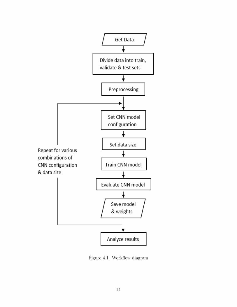
Figure 4.1. Workflow diagram

14

In our method, we started with 8338 images which we have divided into training and

test sets as mentioned above. For the first experiment we use 8000 images for training and

the remaining 338 images for testing. For the next try we decrease the train set by 500

images, setting the training size to 7500 images and the remaining 838 images are used

as test set. We repeat this process with reductions of 500 until we have 2000 images in

the train set and the remaining images in the test set. In each experiment the images are

selected at random and also the training set is further broken into 70% for training and

30% for validating the CNN model.

Table 4.1. CNN Model architecture

Layer type # of filters/nodes Stride Size Activation

Conv2D layer 1-32 filters 1 3x3 reluMax pooling layer 2 2x2

Conv2D layer 1-32 filters 1 3x3 reluMax pooling layer 2 2x2

FlattenFully connected layer 8-64 nodes relu

DropoutFully connected layer 1 node sigmoid

For each of the datasets created above we create CNN architectures with varying convo-

lutional layer filters and number of nodes in the fully connected layer. As seen in table 4.1,

the input image of 200x200 RGB image is fed into the model through a two-dimensional

convolutional layer with varying number of filters from 1 to 32. Each filter is of 3x3 size,

with a default stride value of 1, and activation function relu. The resulting feature map is

pushed onto a max-pooling layer with pooling size 2x2 and stride 2, reducing the dimen-

sionality of the network by 75%. This combination of convolutional layer and max pooling

layer is repeated one more time. After these layers, the model is guaranteed to learn the

important features and these learnt features need to be classified. This classification is done

by a pair of fully connected layers. The first one with 8-64 nodes and relu actiavtion and

the last layer with 1 node and sigmoid activation. This last fully connected layer outputs

15

the prediction of the input image.

We repeat the process five times for every combination of dataset size and configuration

with random splits of the train-validation-test to validate the learning ability of the model

and show that the results are not image dependent. We report the accuracies at each stage

and compare them. It is interesting to study the accuracy as compared to the complexity

of the model and input data size.

4.2. Pre-processing

This the zeroth step in any data science problem since in real life applications, datasets

are seldom clean and ready to be analyzed.

In our experiment, we initially faced problems like, under-sampling, and over-fitting.

We have identified that the causes of the problems were, (a) not enough data, and (b) too

many features. To deal with these problems we first augmented the data by using 180

derivatives of each image (rotating the original ones by 1-degree). Also, we have applied

pixel dimension reduction by identifying the object in the image and cropping it to a

200x200 pixel image. We also discarded the images which do not have a full object in

them and ended up with a total of 8338 with both classes combined. Figures 4.2 show the

resulting images of our dataset after the pre-processing has occurred.

(a) Pre-processed Pupae (b) Pre-processed Instar

Figure 4.2. Pre-processed Images

16

4.3. File Structure Creation

Now that we have a good dataset, we should structure it properly for conducting our

experiments. This process works as long as there exists an input folder directory with

the images in different classes in it. The following is an automated process to create the

required structure:

1) Reads the images with their labels from the input folder.

2) Creates sub-folders,‘train’, ‘vaidation’, ‘test’.

3) Creates sub-folders for each label namely, ’instar4’ and ’pupae’ under each of the ‘train’,

‘validation’ and ‘test’ folders.

4) Copies the required images into each of the labeled folders. These will later be used for

the training and validation of our models.

5) Creates a ’test’ folder which contains the images used for testing the model created.

The following script is used to request the user input. To do so we need to import the

required ‘tkinter’ package which is a python package containing all the necessary functions

used for all the GUI implementations. First, the ‘tkinter’ pop-up window is displayed, as

shown in figure 4.3, prompting the user to navigate to the folder containing the input data.

Listing 4.1. Request for input directory

import tkinter as tk

root = tk.Tk()

root.withdraw ()

input_data_dir = filedialog.askdirectory(parent=root ,

initialdir="//",title=’Pick_the

directory_containing_input_data ’)

The following code is used for getting the directory to save the data through a ‘tkinter’

pop-up window like the previous one as shown in figure 4.4.

17

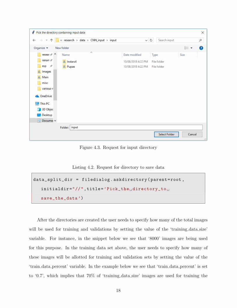
Figure 4.3. Request for input directory

Listing 4.2. Request for directory to save data

data_split_dir = filedialog.askdirectory(parent=root ,

initialdir="//",title=’Pick_the directory_to

save_the_data ’)

After the directories are created the user needs to specify how many of the total images

will be used for training and validations by setting the value of the ‘training data size’

variable. For instance, in the snippet below we see that ‘8000’ images are being used

for this purpose. In the training data set above, the user needs to specify how many of

these images will be allotted for training and validation sets by setting the value of the

‘train data percent’ variable. In the example below we see that ‘train data percent’ is set

to ‘0.7’, which implies that 70% of ‘training data size’ images are used for training the

18

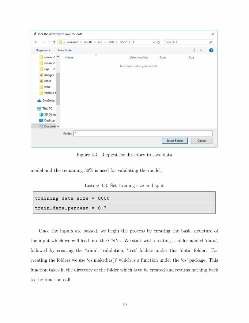
Figure 4.4. Request for directory to save data

model and the remaining 30% is used for validating the model.

Listing 4.3. Set training size and split

training_data_size = 8000

train_data_percent = 0.7

Once the inputs are passed, we begin the process by creating the basic structure of

the input which we will feed into the CNNs. We start with creating a folder named ‘data’,

followed by creating the ‘train’, ‘validation, ‘test’ folders under this ‘data’ folder. For

creating the folders we use ‘os.makedirs()’ which is a function under the ‘os’ package. This

function takes in the directory of the folder which is to be created and returns nothing back

to the function call.

19

Listing 4.4. Creating the basic skeleton for input to CNN.

import os

#data_split_dir is where the ’data’ will be created and

contains train , validation and test folders under it.

data_split_dir = data_split_dir+’/data’

train_data = data_split_dir+’/train’

validation_data = data_split_dir+’/validation ’

test_data = data_split_dir+’/test’

#Creating the ’data’ folder and ’train ’,’validation ’ and ’

test’ folders under it.

os.makedirs(data_split_dir)

os.makedirs(train_data)

os.makedirs(validation_data)

os.makedirs(test_data)

After preparing the skeleton directory, now is the time to get the images from the input

directory and copy them into this skeleton which we have just created. This process begins

by retrieving the names of the classes from the input data and we do so by reading all the

folders inside the input directory. We use another function from the ‘os’ package named

‘listdir()’ which essentially takes in the directory of a folder and returns all of its contents.

Listing 4.5. Retrieve the class names.

input_folders = os.listdir(input_data_dir)

20

Before we start filling the folders with images we still need to create folders for each

class under each of train, validation and test folders. The following snippet illustrates how

this can be achieved through a for-loop implementation where each time the loop gets

executed one of the class’s named folder is created under the train, validation and test

folders.

Listing 4.6. Retrieve the class names.

#Creating the empty folders for filling in the pictures

later

for folder in input_folders:

if(input_folders != ’data’):

os.makedirs(train_data+’/’+folder)

os.makedirs(validation_data+’/’+folder)

os.makedirs(test_data+’/’+folder)

We now finally copy the images from the input folders to respective folders with ap-

propriate amount of images in each of the folders. This step of the process can be further

divided into several parts as follows:

For each of the classes the procedure described below is repeated.

1) Count the number the images associated with this label in the input data.

2) Compute the number of images to be copied into training and validation sets using the

‘train data percent’, ‘training data size’ variables and ‘0.65’ or ‘0.35’ for training and

validation sets, to maintain the original 65%-35% ratio between the two classes.

3) Retrieve the filenames of the images from the input folder and store them into a list

(python’s data structure to save various string variables) using the ‘os.listdir()’ function

and search for only the image files i.e., images with ‘.jpg’ extension.

4) Sort the filenames alphabetically using python’s ‘.sort()’ function.

21

5) Randomize the order to get a randomly split data into all the folders. To randomize the

order ‘random.randint(1,1000)’ is used, which produces a random integer between 1 &

1000 every time it gets executed. Using this random integer the ‘random.seed()’ is set.

6) The random.seed() activates the ‘random’ which is used for shuffling the filenames by

‘random.shuffle(filenames)’ command.

7) Now, for each image, the image is either copied into train, valid or test based on the count

of the train size, valid size computed above. Also, to copy the image the ‘shutil.copy()’

from the ‘shutil’ package is used. This command takes the file to copied and file director

where the file is to be copied, and performs copy function.

Listing 4.7. Fill the folders with appropriate images.

for folder in input_folders:

current_input_folder = input_data_dir+’/’+folder

number_of_images = sum([len(files) for r, d, files

in os.walk(current_input_folder)])

print(number_of_images)

if(folder == ’Pupae’):

train_size = train_data_percent *

training_data_size * 0.65

valid_size = 0.3 * training_data_size * 0.65 +

train_size

else:

train_size = train_data_percent *

training_data_size * 0.35

valid_size = 0.3 * training_data_size * 0.35 +

train_size

train_folder = train_data+’/’+folder+’/’

(Listing 4.7. cont’d.)

22

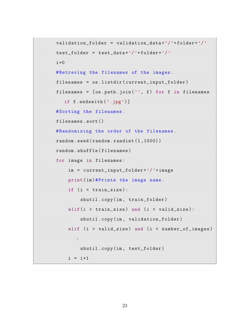
validation_folder = validation_data+’/’+folder+’/’

test_folder = test_data+’/’+folder+’/’

i=0

#Retreving the filenames of the images.

filenames = os.listdir(current_input_folder)

filenames = [os.path.join(’’, f) for f in filenames

if f.endswith(’.jpg’)]

#Sorting the filenames.

filenames.sort()

#Randomizing the order of the filenames.

random.seed(random.randint (1 ,1000))

random.shuffle(filenames)

for image in filenames:

im = current_input_folder+’/’+image

print(im)#Prints the image name.

if (i < train_size):

shutil.copy(im, train_folder)

elif(i > train_size) and (i < valid_size):

shutil.copy(im, validation_folder)

elif (i > valid_size) and (i < number_of_images)

:

shutil.copy(im, test_folder)

i = i+1

23

4.4. Experiment

Once the required data is organized in a structured format we conduct our experi-

ments using the convolutional neural network (CNN) which we have built. The process of

conducting these experiments can be broken down into simple steps as follows :

1) Get input directory.

2) Create and run CNN.

a) Set hyper parameters.

b) Configure CNN.

c) Compile and run CNN.

3) Evaluate the CNN on the test data.

4) Save the results.

The first step is to get the input directory. It can be retrieved by requesting the user to

navigate through the ‘tkinter’ pop-up window (similar to the one in the previous section).

The user will select the ‘data’ folder which was created earlier. Once this is done, we will

set the train and validation directories based on the given input. The script which does

this is as follows:

Listing 4.8. Request input directory.

import tkinter as tk

from tkinter import filedialog

root = tk.Tk()

root.withdraw ()

data_dir = filedialog.askdirectory(parent=root ,initialdir="

//",title=’Pick the directory containing data’)

train_data_dir = data_dir+’/train ’

validation_data_dir = data_dir+’/validation ’

24

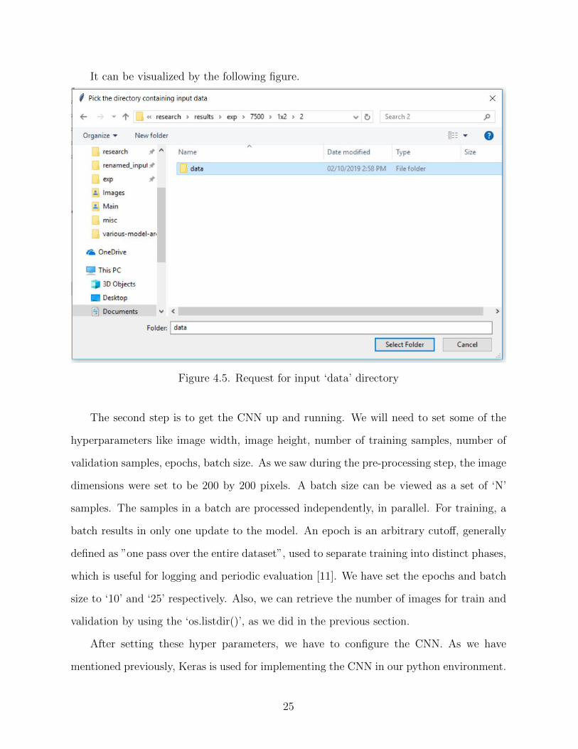
It can be visualized by the following figure.

Figure 4.5. Request for input ‘data’ directory

The second step is to get the CNN up and running. We will need to set some of the

hyperparameters like image width, image height, number of training samples, number of

validation samples, epochs, batch size. As we saw during the pre-processing step, the image

dimensions were set to be 200 by 200 pixels. A batch size can be viewed as a set of ‘N’

samples. The samples in a batch are processed independently, in parallel. For training, a

batch results in only one update to the model. An epoch is an arbitrary cutoff, generally

defined as ”one pass over the entire dataset”, used to separate training into distinct phases,

which is useful for logging and periodic evaluation [11]. We have set the epochs and batch

size to ‘10’ and ‘25’ respectively. Also, we can retrieve the number of images for train and

validation by using the ‘os.listdir()’, as we did in the previous section.

After setting these hyper parameters, we have to configure the CNN. As we have

mentioned previously, Keras is used for implementing the CNN in our python environment.

25

The most important data structure of a Keras implementation is the ‘model’, which is

the aggregate of all CNN layers. There are quite a few options when it comes to the type

of models which one can create. Out of all the models, the Sequential model is the simplest

one of all. Basically the Sequential model is nothing but a linear stack of layers. [11]

Listing 4.9. Initialize model.

from keras.models import Sequential

model = Sequential ()

After initializing the model we will start stacking up the layers using ‘model.add()’

function from the Keras library. This model.add() will be used to add layers, specify

activation function, input shape/size, and has a number of other specialized features, like

‘Dense’ which represents the number of nodes in a particular layer.

Listing 4.10. model.add()

from keras.layers import Dense

# input: 200 x200 images with 3 channels -> (200, 200, 3)

tensors.

# this applies 32 convolution filters of size 3x3 each.

model.add(Conv2D (32, (3, 3), input_shape =(200 ,200 ,3)))

model.add(Activation(’relu’))

model.add(MaxPooling2D(pool_size =(2, 2)))

model.add(Flatten ())

model.add(Dropout (0.5))

In the above script we can observe that the first add function is trying to add a two

dimensional convolutional layer with 32 convolutional filters. This Conv2D layer creates a

convolution kernel that is convolved with the layer input to produce a tensor of outputs.

26

The second add function is specifying the activation function as ‘relu’ to the previously

added Conv2D layer. ‘relu’ is short for rectified linear unit which is one of the most

commonly used activation functions in all types of neural networks.

The third add function is adding a max pooling layer which is very common to observe

between two successive CNN layers. The function of pooling layer is to operate indepen-

dently on each depth slice of the input and re-sizes it spatially. In simpler words, it acts

as a filter which takes in an input matrix (usually 2x2 size) and returns maximum value of

the matrix.

Next add function is used to flatten out the convoluted layers in the CNN architecture.

This flattening is the essential step of CNN architecture which converts CNN architecture

to fully connected ANN architecture. This ANN is actually used for classification purposes.

The last add function is used to add a dropout layer. These layers are primarily used

to combat the problem of overfitting where after a certain moment in training this layer

would drop out a random set of activations in that layer by setting them to zero. This

helps the model not to fit the weights too much. The model just memorizes the data and

not essentially generalize (to find patterns) on data to actually learn the data and perform

a good classification task [12].

Listing 4.11. Data preparation for training input

#We use train_generator variable for getting images for the

input directory to the model

train_generator = ImageDataGenerator ().flow_from_directory(

train_data_dir ,

target_size =(img_width , img_height),

batch_size=batch_size ,

class_mode=’binary ’)

27

‘ImageDataGenerator()’ is a Keras function which is used for generating more samples

of each single image from the input stream. This function is useful when the input data

size is too small for solving the problem. The newly generated images can be obtained by

rotating, translating, flipping either vertically or horizontally, etc. In our case as we did

this in pre-processing phase and we don’t use it again here.

‘flow from directory()’ is another Keras function which acts as an input data pipeline.

In other words, this function is used for getting the input stream of images into the model

we created.

Listing 4.12. Model summary

model.summary ()

When using deep learning, it is useful to understand the different layers present in

the network and how they are organized. This can be visualized by the ‘summary()’,

which prints the model’s architecture along with the total parameters (trainable and none-

trainable) at each layer. An example of the model’s summary can be observed in Figure

4.6.

The last step of the training phase and probably one of the most important step is to

save the results. The functions ‘save’ and ‘save weights’ save the model and its weights

respectively into a ‘.h5’ file. By default these files are saved at the working directory,

although you can pass a target directory as a parameter for saving them at a different

location.

Listing 4.13. Save model and weights

model.save(results_path+’model.h5’)

model.save_weights(results_path+’weights.h5’)

28

Figure 4.6. Model summary

29

Chapter 5.Results

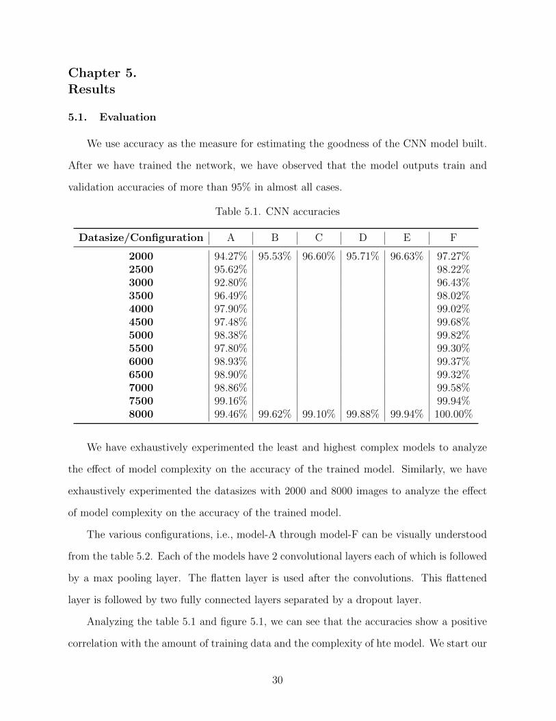
5.1. Evaluation

We use accuracy as the measure for estimating the goodness of the CNN model built.

After we have trained the network, we have observed that the model outputs train and

validation accuracies of more than 95% in almost all cases.

Table 5.1. CNN accuracies

Datasize/Configuration A B C D E F

2000 94.27% 95.53% 96.60% 95.71% 96.63% 97.27%2500 95.62% 98.22%3000 92.80% 96.43%3500 96.49% 98.02%4000 97.90% 99.02%4500 97.48% 99.68%5000 98.38% 99.82%5500 97.80% 99.30%6000 98.93% 99.37%6500 98.90% 99.32%7000 98.86% 99.58%7500 99.16% 99.94%8000 99.46% 99.62% 99.10% 99.88% 99.94% 100.00%

We have exhaustively experimented the least and highest complex models to analyze

the effect of model complexity on the accuracy of the trained model. Similarly, we have

exhaustively experimented the datasizes with 2000 and 8000 images to analyze the effect

of model complexity on the accuracy of the trained model.

The various configurations, i.e., model-A through model-F can be visually understood

from the table 5.2. Each of the models have 2 convolutional layers each of which is followed

by a max pooling layer. The flatten layer is used after the convolutions. This flattened

layer is followed by two fully connected layers separated by a dropout layer.

Analyzing the table 5.1 and figure 5.1, we can see that the accuracies show a positive

correlation with the amount of training data and the complexity of hte model. We start our

30

Figure 5.1. Accuracies for various configurations

experiments with training data size of 2000 images and increase them upto 8000 with 500

increments. Also, we have increasing complexities of models from model-A through model-

F. It is interesting to compare the average time taken for training of various architectures.

The most simple CNN model with 2000 training images takes about 240 seconds, while the

most complex CNN model with 8000 training images takes about 2100 seconds. Also, we

see an increasing trend when we either increase the number of training images or increase

the complexity of the CNN model.

Also, we observed that the test accuracies are always similar to the train and validation

accuracies, which is greater than 95%. Occasionally we have seen that for a particular

experiment, the model overfits the data leaving us with huge gaps between train, test

31

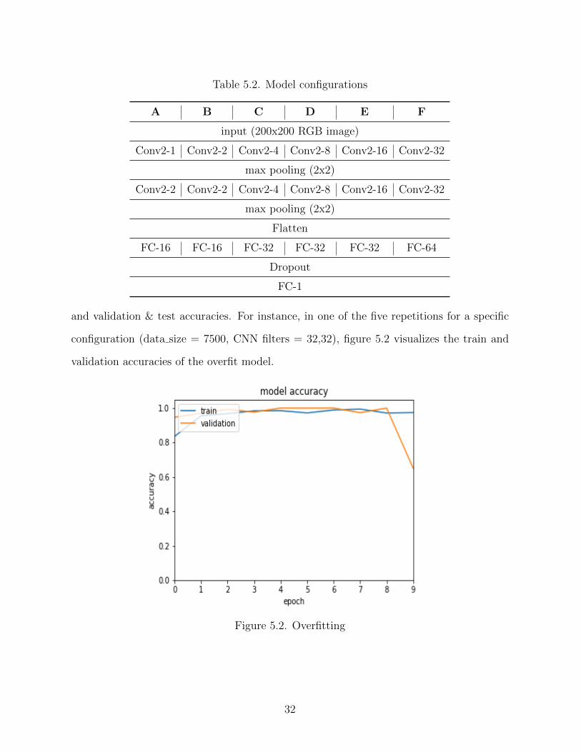
Table 5.2. Model configurations

A B C D E F

input (200x200 RGB image)

Conv2-1 Conv2-2 Conv2-4 Conv2-8 Conv2-16 Conv2-32

max pooling (2x2)

Conv2-2 Conv2-2 Conv2-4 Conv2-8 Conv2-16 Conv2-32

max pooling (2x2)

Flatten

FC-16 FC-16 FC-32 FC-32 FC-32 FC-64

Dropout

FC-1

and validation & test accuracies. For instance, in one of the five repetitions for a specific

configuration (data size = 7500, CNN filters = 32,32), figure 5.2 visualizes the train and

validation accuracies of the overfit model.

Figure 5.2. Overfitting

32

5.2. Image Prediction Algorithm

Besides the analysis of the model with respect to different sizes and architecture, the

goal of this thesis, as mentioned earlier, was to create an automatic prediction tool based

on machine learning. We make use of the saved model architecture and model weights to

reconstruct the model as required to make predictions based on the new test images. We

automated this process for predictions as follows:

1) Read the directory which contains the test images.

2) Create a folder ’predictions’ in the same directory as the test images folder.

3) Create a folder under ’predictions’ for each class, namely, ‘Instar4’, ‘Pupae’ (in our

case).

4) Run the model against these test images to produce predictions which are saved in a

.csv file.

5) A copy of image is saved under their respective labeled folder under the folder named

‘predictions’.

This tool is carefully built by keeping in mind that it can easily be modified into a

solution for any image classification problem. For instance, one application could be to

use this tool for classifying inter-mosquito species. It can even be used to classify different

objects with minute differences such as other stages of mosquito life-cycle like, instar1,

instar2, instar3, which is one of the plausible future works.

33

Chapter 6.Conclusion

In this thesis, we have investigated the use of Convolutional Neural Networks in clas-

sifying two stages of a particular mosquito species’ life cycle namely, Instar4 and Pupae.

We believe we have achieved our main goal to clearly explain the complex methodology

by breaking it down into simple concepts. Furthermore, we have explored various model

configurations with different data sizes and statistically validated our results by repeating

the experiments multiple times. We have achieved a maximum of 100% accuracy in some

runs, with the majority of the accuracy scores being more than 95%.

This thesis is an example of how powerful the Convolutional Neural Networks can be in

the field of Entomology and we hope the results will motivate other researchers to explore

this methodology further and use it for solving similar image classification problems in their

fields.

There are multiple directions in which we would like to extend our research. For

example, one of our immediate goals will be to explore alternative classification algorithms

like a forward feed neural network or Support Vector Machines and perhaps some ensemble

methods, and compare them with ours. Although we believe CNN’s are best suited for this

analysis, they usually take a lot of time for training. It would be interesting to compare

the accuracies, time taken and other metrics for all these plausible methods to identify the

best model in terms of both accuracy and time.

It is also interesting to extend this binary classification into a categorical problem by

considering all the other stages of the life cycle, right from the first stage instars to fully

grown mosquitoes. This new problem would be very complicated compared to the existing

problem as the various stages of instars are difficult to work with. For instance, one of the

problems would be that instar-3 and instar-4 look exactly the same except for the size of

the body relative to each other. This relative sizes is not a standard feature which can

be used for classification. Another challenge that can be faced is that instar-1 are almost

34

invisible and we anticipate that the object might either not be picked by the model or the

object might be lost during the processing of images.

All the codes for the research are publicly available in github in the following link:

https://www.github.com/sumanth-vissamsetty/Mosquito-image-classification

35

References

[1] Anaconda. https://www.anaconda.com/distribution/.

[2] Convolutional neural networks. http://cs231n.github.io/convolutional-networks/.

[3] Opencv - open source computer vision library. https://docs.opencv.org/3.4.1/d1/dfb/intro.html/.

[4] Scikit-learn: A python package with machine learning tools. https://scikit-learn.org/stable/.

[5] Spyder. https://www.spyder-ide.org/.

[6] Python programming language, 2001. https://www.python.org.

[7] Numpy package, 2005. www.numpy.org/.

[8] Pandas: powerful python data analysis toolkit, 2011. https://pandas.pydata.org/pandas-docs/stable/.

[9] Geron Aurelien, Hands-on machine learning with scikit-learn & tensorflow, Oreilly, 2017.

[10] Gustavo E Batista, Eamonn J Keogh, Agenor Mafra-Neto, and Edgar Rowton, Sigkdd demo: sensorsand software to allow computational entomology, an emerging application of data mining, Proceed-ings of the 17th acm sigkdd international conference on knowledge discovery and data mining, 2011,pp. 761–764.

[11] Francois Chollet et al., Keras: The python deep learning library, 2015. https://keras.io.

[12] Adit Deshpande, A-beginner’s-guide-to-understanding-convolutional-neural-networks (2017). https:

//adeshpande3.github.io/adeshpande3.github.io/A-Beginner’s-Guide-To-Understanding-Convolutional-Neural-Networks-Part-2/.

[13] Masataka Fuchida, Thejus Pathmakumar, Rajesh Mohan, Ning Tan, and Akio Nakamura, Vision-based perception and classification of mosquitoes using support vector machine, Applied Sciences 7(2017), no. 1, 51.

[14] Alex Krizhevsky, Ilya Sutskever, and Geoffrey E Hinton, Imagenet classification with deep convolu-tional neural networks, Advances in neural information processing systems, 2012, pp. 1097–1105.

[15] Mona Minakshi, A machine learning framework to classify mosquito species from smart-phone images,Master’s Thesis, 2018.

[16] Jurgen Schmidhuber, Deep learning in neural networks: An overview, CoRR abs/1404.7828 (2014),available at 1404.7828.

[17] Matthew D Zeiler and Rob Fergus, Visualizing and understanding convolutional networks, Europeanconference on computer vision, 2014, pp. 818–833.

36

Vita

Sumanth Vissamsetty is from Hyderabad, India, where he has spent all his life before he

decided to pursue his masters at LSU. He received his Bachelors in Computer Science from

GITAM University in Hyderabad. His passion towards machine learning and programming

motivated him to continue his education and he started his Masters degree at LSU in Com-

puter Science in the year 2016. His primary interests include Machine Learning, Databases,

and Data Analytics.

37