Morphology, dynamics and plasma parameters of plumes and inter-plume regions in solar coronal holes

arX

iv:1

103.

4481

v1 [

astr

o-ph

.SR

] 2

3 M

ar 2

011

Morphology, dynamics and plasma parameters of plumes andinter-plume regions in solar coronal holes

K. Wilhelm · L. Abbo · F. Auchere · N. Barbey · L. Feng · A.H. Gabriel · S. Giordano ·

S. Imada · A. Llebaria · W.H. Matthaeus · G. Poletto · N.-E. Raouafi · S.T. Suess ·

L. Teriaca · Y.-M. Wang

Received: 18 March 20101

DOI 10.1007/s00159-01100035-7

Abstract Coronal plumes, which extend from solar coronal holes (CH) into the high coronaand—possibly— into the solar wind (SW), can now continuously be studied with moderntelescopes and spectrometers on spacecraft, in addition to investigations from the ground,in particular, during total eclipses. Despite the large amount of data available on theseprominent features and related phenomena, many questions remained unanswered as to theirgeneration and relative contributions to the high-speed streams emanating from CHs. Anunderstanding of the processes of plume formation and evolution requires a better knowledgeof the physical conditions at the base of CHs, in plumes and in the surrounding inter-plumeregions (IPR). More specifically, information is needed on the magnetic field configuration, theelectron densities and temperatures, effective ion temperatures, non-thermal motions, plumecross-sections relative to the size of a CH, the plasma bulk speeds, as well as any plume sig-natures in the SW. In spring 2007, the authors proposed a study on “Structure and dynamicsof coronal plumes and inter-plume regions in solar coronal holes” to the International SpaceScience Institute (ISSI) in Bern to clarify some of these aspects by considering relevant ob-servations and the extensive literature. This review summarizes the results and conclusionsof the study. Stereoscopic observations allowed us to include three-dimensional reconstruc-tions of plumes. Multi-instrument investigations carried out during several campaigns ledto progress in some areas, such as plasma densities, temperatures, plume structure and therelation to other solar phenomena, but not all questions could be answered concerning thedetails of plume generation process(es) and interaction with the SW.

Keywords Sun · Corona · Coronal holes · Coronal plumes · Inter-plume regions · Solar wind————————————K. Wilhelm (corresponding author), L. Feng∗, L. TeriacaMax-Planck-Institut fur Sonnensystemforschung37191 Katlenburg-Lindau, Germanye-mail: [email protected]; fax: +49 5556 979 240; tel.: +49 5556 979 423∗ also at Purple Mountain Observatory, Chinese Academy of Sciences210008 Nanjing, China, e-mail: [email protected]

L. Abbo, S. GiordanoINAF – Osservatorio Astronomico di Torinovia Osservatorio 20, 10025 Pino Torinese, Italy

F. Auchere, N. Barbey, A.H. GabrielInstitut d’Astrophysique SpatialeUniversite Paris XI, batiment 121, 91405 Orsay, France

S. ImadaInstitute of Space and Astronautical Science, Japan Aerospace Exploration Agency

1

3-1-1 Yoshinodai, Sagamihara-shi, Kanagawa, 229-8510, Japan

A. LlebariaObservatoire Astronomique de Marseille-Provence, Laboratoire d’Astrophysique de MarseillePole de l’Etoile Site de Chateau-Gombert38, rue Frederic Joliot–Curie, 13388 Marseille Cedex 13, France

W.H. MatthaeusBartol Research Institute and Department of Physics and AstronomyUniversity of Delaware, Newark, DE 19716, USA

G. PolettoOsservatorio Astrofisico di ArcetriLargo Enrico Fermi 5, 50125 Firenze, Italy

N.-E. RaouafiJohns Hopkins University, Applied Physics Laboratory11100 Johns Hopkins Road, Laurel, MD 20723-6099, USA

S.T. SuessNational Space Science and Technology Center320 Sparkman Drive, Huntsville, AL 35805, USA

Y.-M. WangCode 7672, E. O. Hulburt Center for Space ResearchNaval Research LaboratoryWashington, DC 20375-5352, USA

Contents1 Introduction 3

2 Instrumentation 5

2.1 Ground-based systems . . . . . . . . . . . . . . . . . . . . . . . . . . . . . . . . . . . . . . . . . 52.2 Space systems . . . . . . . . . . . . . . . . . . . . . . . . . . . . . . . . . . . . . . . . . . . . . . . 5

2.2.1 Ulysses . . . . . . . . . . . . . . . . . . . . . . . . . . . . . . . . . . . . . . . . . . . . . . . 62.2.2 Remote-sensing instrumentation . . . . . . . . . . . . . . . . . . . . . . . . . . . . . . . 7

2.3 Eclipse and other campaigns . . . . . . . . . . . . . . . . . . . . . . . . . . . . . . . . . . . . . . 92.3.1 Eclipse campaign 2006 . . . . . . . . . . . . . . . . . . . . . . . . . . . . . . . . . . . . . 92.3.2 Multi-instrument campaign 2008 . . . . . . . . . . . . . . . . . . . . . . . . . . . . . . . 9

3 Morphology of plumes in coronal holes 10

3.1 Magnetic field configuration . . . . . . . . . . . . . . . . . . . . . . . . . . . . . . . . . . . . . . 10

3.2 Plume geometry and dimensions . . . . . . . . . . . . . . . . . . . . . . . . . . . . . . . . . . . 14

4 Dynamics 18

4.1 Life cycle of plumes . . . . . . . . . . . . . . . . . . . . . . . . . . . . . . . . . . . . . . . . . . . 204.2 Waves and turbulence in plumes and inter-plume regions . . . . . . . . . . . . . . . . . . . . 20

4.3 Outflows in plumes, inter-plume regions and coronal holes . . . . . . . . . . . . . . . . . . . 22

5 Plasma conditions in coronal holes 26

5.1 Electron densities in plumes and inter-plume regions . . . . . . . . . . . . . . . . . . . . . . 275.2 Plasma temperatures and non-thermal motions . . . . . . . . . . . . . . . . . . . . . . . . . . 32

5.2.1 Electron temperature . . . . . . . . . . . . . . . . . . . . . . . . . . . . . . . . . . . . . . 325.2.2 Line profiles and effective ion temperatures . . . . . . . . . . . . . . . . . . . . . . . . 395.2.3 Ion temperatures and non-thermal motions . . . . . . . . . . . . . . . . . . . . . . . . 42

5.3 Elemental abundances and first ionization potentials . . . . . . . . . . . . . . . . . . . . . . 43

6 Relations of plumes to other solar phenomena 45

6.1 Chromospheric network . . . . . . . . . . . . . . . . . . . . . . . . . . . . . . . . . . . . . . . . . 456.2 Bright points . . . . . . . . . . . . . . . . . . . . . . . . . . . . . . . . . . . . . . . . . . . . . . . 46

6.3 Spicules, macrospicules and jets . . . . . . . . . . . . . . . . . . . . . . . . . . . . . . . . . . . 46

2

6.4 Fast solar wind and the Heliosphere . . . . . . . . . . . . . . . . . . . . . . . . . . . . . . . . . 496.5 Density and magnetic-field fluctuations . . . . . . . . . . . . . . . . . . . . . . . . . . . . . . . 50

7 Classification 51

8 Plume models and generation processes 52

8.1 Plume formation and decay . . . . . . . . . . . . . . . . . . . . . . . . . . . . . . . . . . . . . . 52

8.2 Beam and network plumes . . . . . . . . . . . . . . . . . . . . . . . . . . . . . . . . . . . . . . . 558.3 Forward modeling . . . . . . . . . . . . . . . . . . . . . . . . . . . . . . . . . . . . . . . . . . . . 55

9 Conclusions 55

A List of acronyms and abbreviations 58

1 Introduction

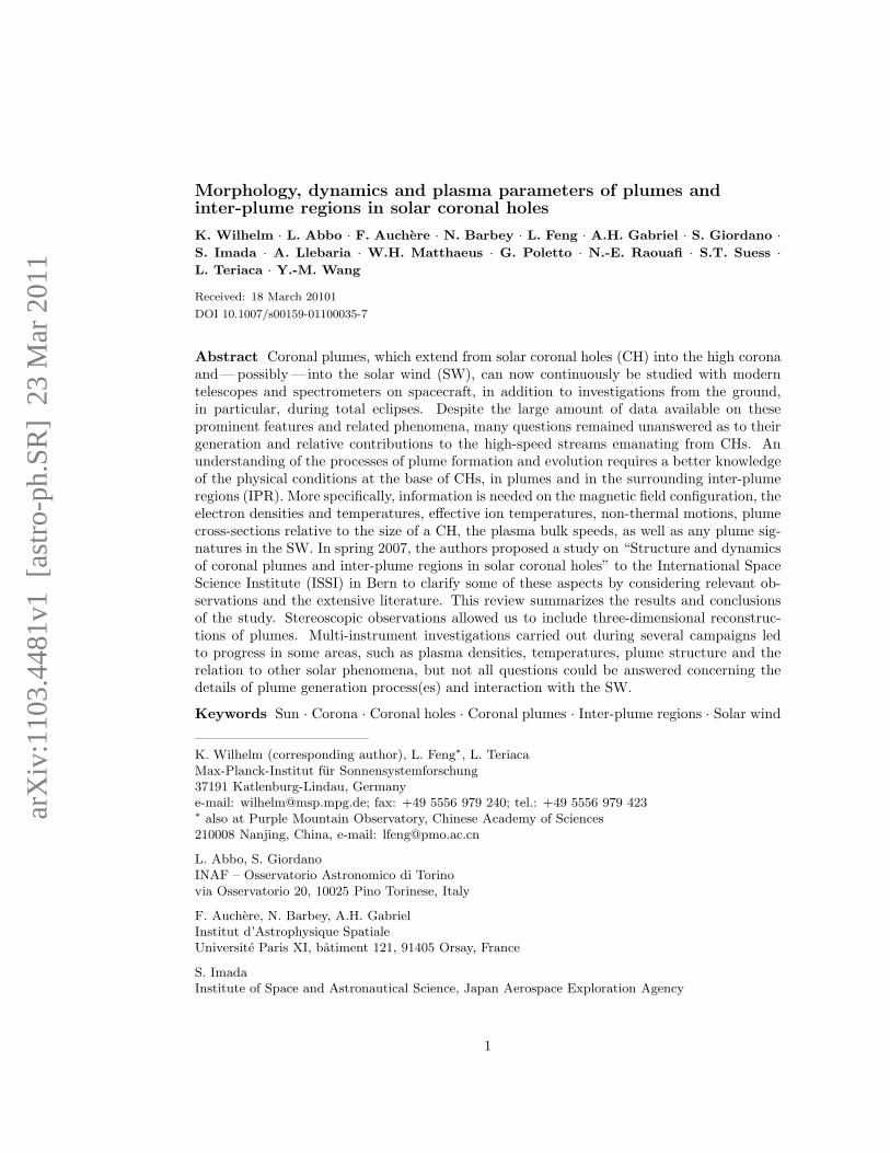
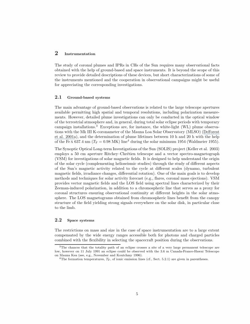
Coronal plumes, extending as bright, narrow structures from the solar chromosphere intothe high corona, have long been seen as fascinating phenomenon during total eclipses (cf.,e.g., van de Hulst 1950a, b), and can now be observed with telescopes and spectrometers onspacecraft without interruption. They are prominent features of the solar corona, both invisible and ultraviolet (UV)1 radiation, and are rooted in coronal holes (CH). A spectacularimage of the solar corona during an eclipse is shown in Fig. 1. Notice— in the context ofour study—the plumes at the N and S poles as well as the bright coronal material in theN that would interfere with any line-of-sight (LOS) observations of the plume configuration.In order to demonstrate the relation between coronal plumes and the northern and southernpolar coronal holes (PCH), the occulted disk of the Sun is filled with an extreme-ultraviolet(EUV) image taken by the EUV Imaging Telescope (EIT) (cf., Sect. 2.2.2).

Van de Hulst (1950b) confirmed Alfven’s conclusion that polar coronal plumes (rays in theold terminology, cf., Sect. 7) coincided with “open” magnetic lines of force and thus outlinethe general magnetic field of the Sun. PCHs are best developed during the minimum of thesolar activity. Consequently, many plume and PCH studies were carried out after the launchof the Solar and Heliospheric Observatory (SOHO) under very quiet conditions of the Sun in1996 and 1997, followed by additional observations during the recent minimum of the 11 yearsunspot cycle. Plumes are also observed in non-polar CHs (Del Zanna and Bromage 1999; DelZanna et al. 2003; Wang and Muglach 2008). Most of the past observations have, however,been related to polar plumes, and they will be the main topic of this study proposed to theInternational Space Science Institute (ISSI), Bern, in March 2007. It was motivated by thefact that no undisputed theoretical concept was available for the formation of plumes, andeven many observational facts appeared to be in conflict with each other. In particular, thethree-dimensional (3D) structure of plumes and their dynamical properties, along with thoseof the inter-plume regions (IPR) had been under discussion.

We, the members of the study team on “Structure and dynamics of coronal plumes and inter-plume regions” reviewed, without any claim to be exhaustive, the wealth of observational dataavailable on coronal plumes and their environment.2 This, together with the analyses carried

1A list of acronyms and abbreviations is compiled in Appendix A.2Taking advantage of the prevailing solar minimum conditions at the beginning of the proposed study,

some additional plume observations had also been suggested and were carried out in 2007 and 2008. Theanalysis of these data sets is not yet completed, but some campaign information and results are included inthis report.

3

Figure 1: The solar corona during the total eclipse on 1 August 2008 observed from Mongolia.The corona at solar minimum conditions has wide PCHs with reduced radiation, open magneticfield lines and many plume structures. At lower latitudes closed field-line regions dominate thecorona and extend into coronal streamers (from Pasachoff et al. 2009; composite eclipse image by M.Druckmuller, P. Aniol and V. Rusin). An image in 19.5 nm of the solar disk taken from EIT/SOHOat the time of the eclipse has been inserted into the shadow of the Moon.

out in the past, allowed us to answer a number of questions formulated in the proposal phaseof the study. These questions will be repeated in the appropriate sections, and we will restrictthe discussion to these specific topics as a general review on coronal plumes taking all aspectsinto account will appear in Living Reviews (Poletto, to be submitted). We can also refer thereader to earlier plume studies, e.g., by Saito (1965a), Newkirk and Harvey (1968), Ahmadand Withbroe (1977), Del Zanna et al. (1997), DeForest et al. (1997) and Koutschmy andBocchialini (1998). Reference can also be made to reviews on the extended corona of the Sun(Kohl et al. 2006) and to solar UV spectroscopy (Wilhelm et al. 2004, 2007). The interestin coronal plumes led to two special sessions in the past, namely, “Solar jets and coronalplumes”, Guadeloupe, 23 – 26 February 1998 (ESA SP-421, 1998, T-D Guyenne, ed.) and“Solar polar plumes” at the 2nd Asia Oceania Geoscience (AOGS) Conference, Singapore, 20– 24 June 2005.

It might be appropriate to mention from the outset that not all questions could be answeredconclusively. Future investigations utilizing multi-instrument, high-resolution observationswill be needed to complete the task.

4

2 Instrumentation

The study of coronal plumes and IPRs in CHs of the Sun requires many observational factsobtained with the help of ground-based and space instruments. It is beyond the scope of thisreview to provide detailed descriptions of these devices, but short characterizations of some ofthe instruments mentioned and the cooperation in observational campaigns might be usefulfor appreciating the corresponding investigations.

2.1 Ground-based systems

The main advantage of ground-based observations is related to the large telescope aperturesavailable permitting high spatial and temporal resolutions, including polarization measure-ments. However, detailed plume investigations can only be conducted in the optical windowof the terrestrial atmosphere and, in general, during total solar eclipse periods with temporarycampaign installations.3 Exceptions are, for instance, the white-light (WL) plume observa-tions with the Mk III K-coronameter of the Mauna Loa Solar Observatory (MLSO) (DeForestet al. 2001a), and the determination of plume lifetimes between 10 h and 20 h with the helpof the Fex 637.4 nm (TF = 0.98 MK) line4 during the solar minimum 1954 (Waldmeier 1955).

The Synoptic Optical Long-term Investigations of the Sun (SOLIS) project (Keller et al. 2003)employs a 50 cm aperture Ritchey–Chretien telescope and a vector spectro-magnetograph(VSM) for investigations of solar magnetic fields. It is designed to help understand the originof the solar cycle (complementing helioseismic studies) through the study of different aspectsof the Sun’s magnetic activity related to the cycle at different scales (dynamo, turbulentmagnetic fields, irradiance changes, differential rotation). One of the main goals is to developmethods and techniques for solar activity forecast (e.g., flares, coronal mass ejections). VSMprovides vector magnetic fields and the LOS field using spectral lines characterized by theirZeeman-induced polarization, in addition to a chromospheric line that serves as a proxy forcoronal structures ensuring observational continuity at different heights in the solar atmo-sphere. The LOS magnetograms obtained from chromospheric lines benefit from the canopystructure of the field yielding strong signals everywhere on the solar disk, in particular closeto the limb.

2.2 Space systems

The restrictions on mass and size in the case of space instrumentation are to a large extentcompensated by the wide energy ranges accessible both for photons and charged particlescombined with the flexibility in selecting the spacecraft position during the observations.

3The chances that the totality path of an eclipse crosses a site of a very large permanent telescope arelow, however on 11 July 1991 an eclipse could be observed with the 3.6 m Canada-France-Hawai Telescopeon Mauna Kea (see, e.g., November and Koutchmy 1996).

4The formation temperatures, TF, of ionic emission lines (cf., Sect. 5.2.1) are given in parentheses.

5

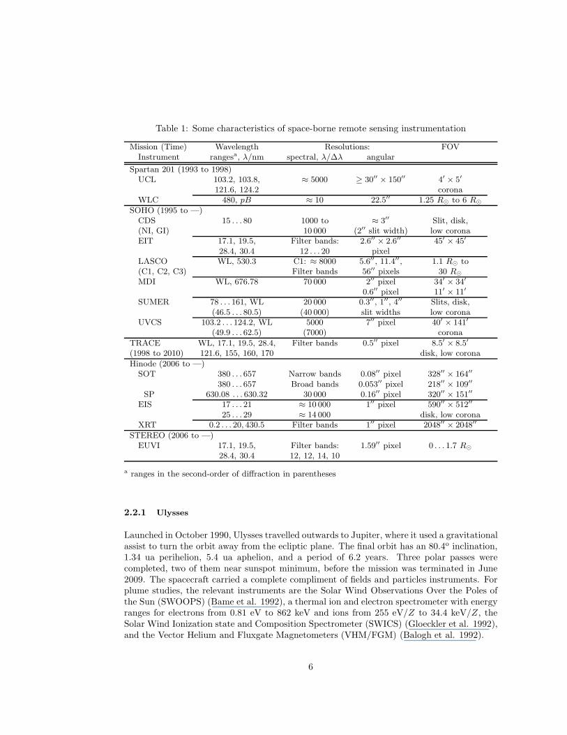
Table 1: Some characteristics of space-borne remote sensing instrumentation

Mission (Time) Wavelength Resolutions: FOVInstrument rangesa, λ/nm spectral, λ/∆λ angular

Spartan 201 (1993 to 1998)UCL 103.2, 103.8, ≈ 5000 ≥ 30′′ × 150′′ 4′ × 5′

121.6, 124.2 coronaWLC 480, pB ≈ 10 22.5′′ 1.25 R⊙ to 6 R⊙

SOHO (1995 to —)CDS 15 . . . 80 1000 to ≈ 3′′ Slit, disk,(NI, GI) 10 000 (2′′ slit width) low coronaEIT 17.1, 19.5, Filter bands: 2.6′′ × 2.6′′ 45′ × 45′

28.4, 30.4 12 . . . 20 pixelLASCO WL, 530.3 C1: ≈ 8000 5.6′′, 11.4′′, 1.1 R⊙ to(C1, C2, C3) Filter bands 56′′ pixels 30 R⊙

MDI WL, 676.78 70 000 2′′ pixel 34′ × 34′

0.6′′ pixel 11′ × 11′

SUMER 78 . . . 161, WL 20 000 0.3′′, 1′′, 4′′ Slits, disk,(46.5 . . . 80.5) (40 000) slit widths low corona

UVCS 103.2 . . . 124.2, WL 5000 7′′ pixel 40′ × 141′

(49.9 . . . 62.5) (7000) corona

TRACE WL, 17.1, 19.5, 28.4, Filter bands 0.5′′ pixel 8.5′ × 8.5′

(1998 to 2010) 121.6, 155, 160, 170 disk, low corona

Hinode (2006 to —)SOT 380 . . . 657 Narrow bands 0.08′′ pixel 328′′ × 164′′

380 . . . 657 Broad bands 0.053′′ pixel 218′′ × 109′′

SP 630.08 . . . 630.32 30 000 0.16′′ pixel 320′′ × 151′′

EIS 17 . . . 21 ≈ 10 000 1′′ pixel 590′′ × 512′′

25 . . . 29 ≈ 14 000 disk, low coronaXRT 0.2 . . . 20, 430.5 Filter bands 1′′ pixel 2048′′ × 2048′′

STEREO (2006 to —)EUVI 17.1, 19.5, Filter bands: 1.59′′ pixel 0 . . . 1.7 R⊙

28.4, 30.4 12, 12, 14, 10

a ranges in the second-order of diffraction in parentheses

2.2.1 Ulysses

Launched in October 1990, Ulysses travelled outwards to Jupiter, where it used a gravitationalassist to turn the orbit away from the ecliptic plane. The final orbit has an 80.4o inclination,1.34 ua perihelion, 5.4 ua aphelion, and a period of 6.2 years. Three polar passes werecompleted, two of them near sunspot minimum, before the mission was terminated in June2009. The spacecraft carried a complete compliment of fields and particles instruments. Forplume studies, the relevant instruments are the Solar Wind Observations Over the Poles ofthe Sun (SWOOPS) (Bame et al. 1992), a thermal ion and electron spectrometer with energyranges for electrons from 0.81 eV to 862 keV and ions from 255 eV/Z to 34.4 keV/Z, theSolar Wind Ionization state and Composition Spectrometer (SWICS) (Gloeckler et al. 1992),and the Vector Helium and Fluxgate Magnetometers (VHM/FGM) (Balogh et al. 1992).

6

SWOOPS returned the temperatures, densities and vector speeds of protons (H+, p), αparticles (He2+) and electrons. Speed changes of a few kilometres per second over a fewseconds could be resolved. SWICS recorded the speed and density of He2+ and the densities,ionization states and speeds of several minor ions of the elements C, O, Ne, Mg, Si and Fe.The data rate of Ulysses was limited by the transmitter power available and the distancefrom the Earth so that expected SWICS plume signatures are at the level of detectability.VH-FGM measured the vector magnetic field at a far higher cadence than SWOOPS.

2.2.2 Remote-sensing instrumentation

Some of the relevant instrument characteristics are listed in Table 1 in order to present acompact and coherent overview of the following missions and their operational periods:– Spartan was a satellite system launched and retrieved by the Space Shuttle on four occasions.It carried the Ultraviolet Coronal Spectrometer (UCS), an externally and internally occultedcoronagraph with a dual spectrograph as well as the White Light Coronagraph (WLC) (Kohlet al. 1995; Guhathakurta and Fisher 1995), a coronagraph with polarimeter for polarizedbrightness, pB, measurements (cf., Sect. 5.1).– SOHO was launched on 2 December 1995 and injected into a halo orbit around the Sun-EarthLagrange point L1 (≈ 0.01 ua sunward of the Earth) on 14 February 1996 (see Domingo etal. 1995 and references therein). The following instruments are of importance in our context:(1) The Coronal Diagnostic Spectrometer (CDS) with normal- and grazing-incidence (NI/GI)spectrometers in the EUV wavelength range. (2) EIT, a full-disk solar imager for observationsin the emission lines Fe ix 17.1 nm (0.71 MK), (Fex 17.5 nm); Fexii 19.5 nm (1.38 MK);Fexv 28.4 nm (2.08 MK); He ii 30.4 nm (81 000 K). (3) The Large Angle and SpectrometerCoronagraph (LASCO), a triple coronagraph (C1, C2, C3) in the visible wavelength regimewith nested FOVs out to heliocentric distances R = 30 R⊙ (1 R⊙ = 696 Mm, the radius of theSun5). C1 observed with a Fabry–Perot interferometer, among other lines, Fexiv 530.3 nm(1.82 MK). C2 and C3 had a set of wideband filters. Most of images were obtained with theorange filter of C2: (540 to 640) nm, and the clear filter of C3: (400 to 850) nm; both used aset of three polarizers (– 60o, 0o, 60o) on specific sequences. (4) The Michelson Doppler Imager(MDI) observes solar oscillations and LOS magnetic fields in the Ni i 678.8 line with a tunableinterferometer. (5) The Solar Ultraviolet Measurements of Emitted Radiation spectrometer(SUMER) measures radiation in the vacuum-ultraviolet (VUV) wavelength range with slitlengths of 120′′ and 300′′ and spatial rasters. (6) The Ultraviolet Coronagraph Spectrometer(UVCS) spectrometers are fed by three occulted telescopes for observations of the extendedsolar corona.– The Transition Region and Coronal Explorer (TRACE), was launched by a Pegasus vehicleinto a Sun-synchronous Earth orbit on 2 April 1998. The spacecraft carried a 30 cm Cassegraintelescope. A typical temporal resolution was 5 s (Handy et al. 1999).– Hinode was launched on 22 September 2006 (Kosugi et al. 2007). The three instrumentson board are: (1) The Solar Optical Telescope (SOT), a 50 cm diffraction-limited Gregoriantelescope (Suematsu et al. 2008) feeding narrow-band and broad-band filter imagers and aspectro-polarimeter (SP). Polarization spectra of the Fe i 630.15 nm and 630.20 nm lines areobtained for high-precision Stokes polarimetry and measurements of the three components

51R⊙ is seen from Earth under an angle of 961′′±15′′, depending on the season. The angle is ≈ 10′′ largerfrom SOHO. A distance of ≈ 720 km in the solar photosphere corresponds to 1′′.

7

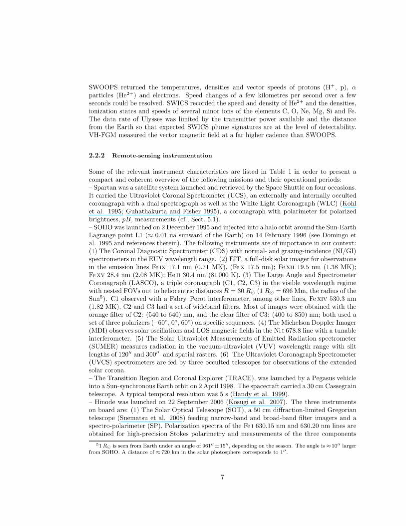
Figure 2: Composite image of the corona during the eclipse of 29 March 2006 built up from SOHOdata (outer frame from LASCO, green rectangle near south pole from SUMER), polarized radiationfrom the EKPol experiment (circular portion from Abbo et al. 2008) and WL ground-based obser-vations (rectangular portion from Koutchmy et al. 2006; obs.: J. Mouette). The solar disk in the17.1 nm band of EIT has been inserted into the shadow of the Moon. The black solid line representsthe operational UVCS slit during the eclipse.

of the magnetic field in the photosphere (Tsuneta et al. 2008a). (2) The EUV ImagingSpectrometer (EIS), a NI stigmatic spectrometer fed by a multi-layer telescope (Culhane etal. 2007), observes prominent emission lines, e.g., Feviii 18.52 nm (0.44 MK), Fexii, Fexiii20.2 nm (1.58 MK) and Fexxiv 19.20 nm (17.0 MK), with four slit or slot widths from1′′ to 266′′. (3) The X-Ray Telescope (XRT), a 30 cm aperture GI telescope with analysisfilters, provides nine X-ray wavelength bands with different lower cut-off energies (Golup etal. 2007).– The Solar Terrestrial Relations Observatory (STEREO), was launched in October 2006near a minimum of solar activity. Two identical spacecraft (STEREO A and B) are driftingapart along the Earth’s orbit and observe the Sun almost simultaneously with the ExtremeUltraviolet Imager (EUVI) telescopes (Wuelser et al. 2004) of the instrument package SunEarth Connection Coronal and Heliospheric Investigation (Secchi) (Howard et al. 2008). Forplume observations, long exposure times and low compression rates are applied to increasethe signal-to-noise ratio.

8

2.3 Eclipse and other campaigns

In particular during total eclipse periods, but also at other times, special plume observingcampaigns have been organized involving many instruments on the ground and in space.Examples are:

2.3.1 Eclipse campaign 2006

Total solar eclipses offer great opportunities to observe the faint solar corona, especially inits inner portions, which are not easily accessible by coronagraphic telescopes, owing to theinstrumentally scattered light. This background is significantly reduced during an eclipse.

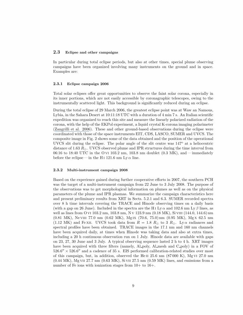
During the total eclipse of 29 March 2006, the greatest eclipse point was at Waw an Namous,Lybia, in the Sahara Desert at 10:11:18 UTC with a duration of 4 min 7 s. An Italian scientificexpedition was organized to reach this site and measure the linearly polarized radiation of thecorona, with the help of the EKPol experiment, a liquid crystal K-corona imaging polarimeter(Zangrilli et al. 2006). These and other ground-based observations during the eclipse werecoordinated with those of the space instruments EIT, CDS, LASCO, SUMER and UVCS. Thecomposite image in Fig. 2 shows some of the data obtained and the position of the operationalUVCS slit during the eclipse. The polar angle of the slit centre was 147o at a heliocentricdistance of 1.63 R⊙. UVCS observed plume and IPR structures during the time interval from06:16 to 18:40 UTC in the Ovi 103.2 nm, 103.8 nm doublet (0.3 MK), and— immediatelybefore the eclipse— in the H i 121.6 nm Lyα line.

2.3.2 Multi-instrument campaign 2008

Based on the experience gained during further cooperative efforts in 2007, the southern PCHwas the target of a multi-instrument campaign from 22 June to 3 July 2008. The purpose ofthe observations was to get morphological information on plumes as well as on the physicalparameters of the plume and IPR plasmas. We summarize the campaign characteristics hereand present preliminary results from XRT in Sects. 5.2.1 and 6.3. SUMER recorded spectraover 8 h time intervals covering the TRACE and Hinode observing times on a daily basis(with a gap on 26 June). Included in the spectra are the H i Lyα and 102.6 nm Ly β lines, aswell as lines from Ovi 103.2 nm, 103.8 nm, Nv 123.9 nm (0.18 MK), Siviii (144.0, 144.6)nm(0.81 MK), Neviii 77.0 nm (0.62 MK), Mg ix (70.6, 75.0) nm (0.95 MK), Mgx 62.5 nm(1.12 MK) and Fexii. UVCS took data from R = 1.8 R⊙ to 3 R⊙. Lyα radiances andspectral profiles have been obtained. TRACE images in the 17.1 nm and 160 nm channelshave been acquired daily, at times when Hinode was taking data and also at extra times,including a 20 h continuous observation run on 1 July. Hinode data are available with gapson 23, 27, 30 June and 3 July. A typical observing sequence lasted 2 h to 4 h. XRT imageshave been acquired with three filters (namely, Al poly, Al mesh and C poly) in a FOV of526.6′′ × 526.6′′ and a cadence of 35 s. EIS performed calibration-related studies over mostof this campaign, but, in addition, observed the He ii 25.6 nm (87 000 K), Mgvi 27.0 nm(0.44 MK), Mgvii 27.7 nm (0.63 MK), Sivii 27.5 nm (0.59 MK) lines, and emissions from anumber of Fe ions with ionization stages from 10+ to 16+.

9

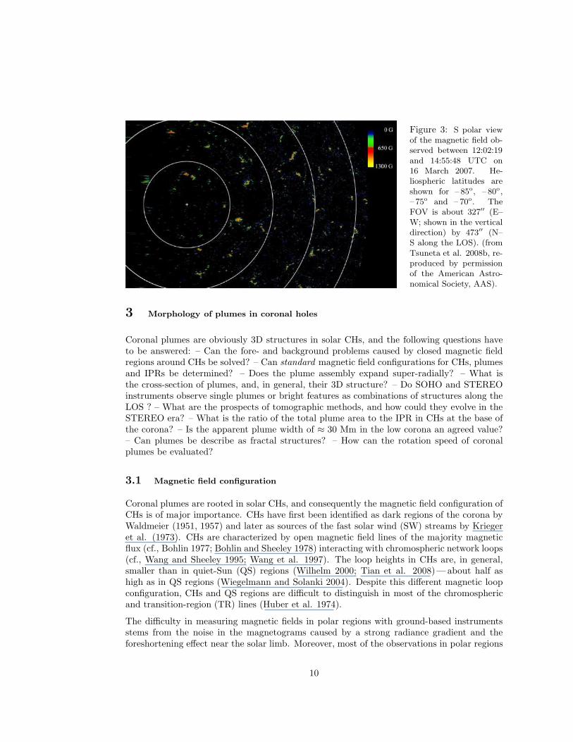
Figure 3: S polar viewof the magnetic field ob-served between 12:02:19and 14:55:48 UTC on16 March 2007. He-liospheric latitudes areshown for – 85o, – 80o,– 75o and – 70o. TheFOV is about 327′′ (E–W; shown in the verticaldirection) by 473′′ (N–S along the LOS). (fromTsuneta et al. 2008b, re-produced by permissionof the American Astro-nomical Society, AAS).

3 Morphology of plumes in coronal holes

Coronal plumes are obviously 3D structures in solar CHs, and the following questions haveto be answered: – Can the fore- and background problems caused by closed magnetic fieldregions around CHs be solved? – Can standard magnetic field configurations for CHs, plumesand IPRs be determined? – Does the plume assembly expand super-radially? – What isthe cross-section of plumes, and, in general, their 3D structure? – Do SOHO and STEREOinstruments observe single plumes or bright features as combinations of structures along theLOS ? – What are the prospects of tomographic methods, and how could they evolve in theSTEREO era? – What is the ratio of the total plume area to the IPR in CHs at the base ofthe corona? – Is the apparent plume width of ≈ 30 Mm in the low corona an agreed value?– Can plumes be describe as fractal structures? – How can the rotation speed of coronalplumes be evaluated?

3.1 Magnetic field configuration

Coronal plumes are rooted in solar CHs, and consequently the magnetic field configuration ofCHs is of major importance. CHs have first been identified as dark regions of the corona byWaldmeier (1951, 1957) and later as sources of the fast solar wind (SW) streams by Kriegeret al. (1973). CHs are characterized by open magnetic field lines of the majority magneticflux (cf., Bohlin 1977; Bohlin and Sheeley 1978) interacting with chromospheric network loops(cf., Wang and Sheeley 1995; Wang et al. 1997). The loop heights in CHs are, in general,smaller than in quiet-Sun (QS) regions (Wilhelm 2000; Tian et al. 2008)—about half ashigh as in QS regions (Wiegelmann and Solanki 2004). Despite this different magnetic loopconfiguration, CHs and QS regions are difficult to distinguish in most of the chromosphericand transition-region (TR) lines (Huber et al. 1974).

The difficulty in measuring magnetic fields in polar regions with ground-based instrumentsstems from the noise in the magnetograms caused by a strong radiance gradient and theforeshortening effect near the solar limb. Moreover, most of the observations in polar regions

10

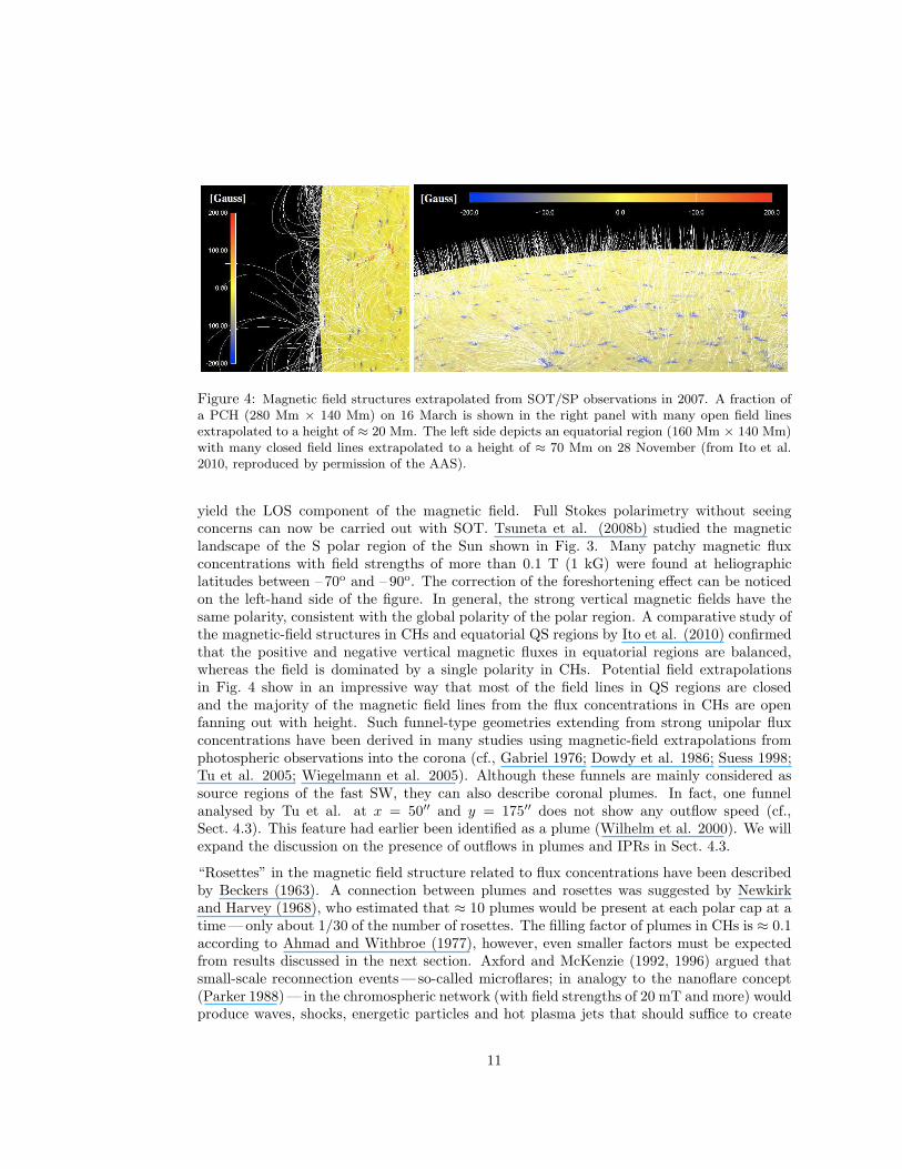
Figure 4: Magnetic field structures extrapolated from SOT/SP observations in 2007. A fraction ofa PCH (280 Mm × 140 Mm) on 16 March is shown in the right panel with many open field linesextrapolated to a height of ≈ 20 Mm. The left side depicts an equatorial region (160 Mm × 140 Mm)with many closed field lines extrapolated to a height of ≈ 70 Mm on 28 November (from Ito et al.2010, reproduced by permission of the AAS).

yield the LOS component of the magnetic field. Full Stokes polarimetry without seeingconcerns can now be carried out with SOT. Tsuneta et al. (2008b) studied the magneticlandscape of the S polar region of the Sun shown in Fig. 3. Many patchy magnetic fluxconcentrations with field strengths of more than 0.1 T (1 kG) were found at heliographiclatitudes between – 70o and – 90o. The correction of the foreshortening effect can be noticedon the left-hand side of the figure. In general, the strong vertical magnetic fields have thesame polarity, consistent with the global polarity of the polar region. A comparative study ofthe magnetic-field structures in CHs and equatorial QS regions by Ito et al. (2010) confirmedthat the positive and negative vertical magnetic fluxes in equatorial regions are balanced,whereas the field is dominated by a single polarity in CHs. Potential field extrapolationsin Fig. 4 show in an impressive way that most of the field lines in QS regions are closedand the majority of the magnetic field lines from the flux concentrations in CHs are openfanning out with height. Such funnel-type geometries extending from strong unipolar fluxconcentrations have been derived in many studies using magnetic-field extrapolations fromphotospheric observations into the corona (cf., Gabriel 1976; Dowdy et al. 1986; Suess 1998;Tu et al. 2005; Wiegelmann et al. 2005). Although these funnels are mainly considered assource regions of the fast SW, they can also describe coronal plumes. In fact, one funnelanalysed by Tu et al. at x = 50′′ and y = 175′′ does not show any outflow speed (cf.,Sect. 4.3). This feature had earlier been identified as a plume (Wilhelm et al. 2000). We willexpand the discussion on the presence of outflows in plumes and IPRs in Sect. 4.3.

“Rosettes” in the magnetic field structure related to flux concentrations have been describedby Beckers (1963). A connection between plumes and rosettes was suggested by Newkirkand Harvey (1968), who estimated that ≈ 10 plumes would be present at each polar cap at atime—only about 1/30 of the number of rosettes. The filling factor of plumes in CHs is ≈ 0.1according to Ahmad and Withbroe (1977), however, even smaller factors must be expectedfrom results discussed in the next section. Axford and McKenzie (1992, 1996) argued thatsmall-scale reconnection events—so-called microflares; in analogy to the nanoflare concept(Parker 1988)— in the chromospheric network (with field strengths of 20 mT and more) wouldproduce waves, shocks, energetic particles and hot plasma jets that should suffice to create

11

the fast SW on open field-line structures (McKenzie et al. 1995).

From WL observations, plumes appear to expand super-radially together with the CHs withaltitude (Saito 1965a; Ahmad and Withbroe 1977; Munro and Jackson 1977; Fisher andGuhathakurta 1995; Koutchmy and Bocchialini 1998). DeForest et al. (1997) found fromSOHO observations that plumes rapidly expand (super-radially with a half-cone angle of 45o)in their lowest height range h = R − 1 R⊙ < 30 Mm to diameters of 20 Mm to 30 Mm, andmore slowly above; the linear expansion ratios of plumes seen in the plane of the sky were 1,3 and 6 at heights of h = (0.05, 4, 14) R⊙, respectively, and 1, 3 and 3 for the backgroundCH. The expansion factor of a plume is also a weak function of the footpoint location in theCH (cf., Goldstein et al. 1996; DeForest et al. 2001b). The CH expansion factor, f(R),for a flux tube with cross-section A is often defined (cf., e.g., Kopp and Holzer 1976) asA(R)/A(R⊙) = (R/R⊙)

2 f(R), where f(R⊙) = 1 and f(R) depends upon the parametersfmax, R1 as well as σ (fmax is the net non-radial divergence, R1 the distance of the mostrapid expansion and σ the range over which it occurs). In this framework, the CH expansionpublished by Cranmer et al. (1999) can be parametrized by the values 6.5, 1.5 R⊙ and0.6 R⊙ of the above parameters, whereas the expansion of DeForest et al. (2001b) can befitted reasonably well by the values 5.65, 1.53 R⊙ and 0.65 R⊙ —after noticing that thequantity

√

f(R) is shown in their Fig. 8. The conclusion was reached that a radial expansionclaimed by some authors (cf., e.g., Woo and Habbal 2000) is inconsistent with observationsin PCHs. The plumes subtend a solar latitude angle of 2o to 2.5o near the limb, which is inagreement with eclipse observations (Newkirk and Harvey 1968). Observations during foureclipse periods showed an average width of 31 Mm (corresponding to 2.6o) at h = 0.05 R⊙

(Hiei et al. 2000). The fraction of plumes wider than 4o or narrower than 2o was ≈ 20 %,each.

As mentioned in Sect. 1, the best observing conditions of coronal plumes exist near theminimum of the activity cycle when the PCHs have their maximum extension from the polesto ± 60◦ solar latitudes (Wang and Sheeley 1990; Banaszkiewicz et al. 1998). In this phase,it is unlikely that neighbouring streamers significantly contaminate the PCH observations.6

The southern CH in Fig. 1 shows an example of such an optimal condition. It is obviousfrom this figure that the plumes diverge super-radially with altitude in the PCHs. Plumesnear the limb appear to converge to points on the solar rotation axis more than half the waybetween the centre of the Sun and the poles (Saito 1965a; Marsch et al. 1997; Boursier andLlebaria 2008). The super-radial expansion could also be confirmed in the 3D reconstructionsusing EUVI data in 2007 (Feng et al. 2009). An example of such a reconstruction is shownin Fig. 5. In addition to the divergence of the plume assembly, the cross-sectional area ofthe plumes expands as well (cf., Casalbuoni et al. 1999; and the discussion in the previousparagraph). According to model calculations, most of this expansion occurs at the base below≈ 35 Mm, where the plumes grow in diameter from ≈ 3 Mm by nearly a factor of ten. Inthe regime of low β (the ratio of the plasma pressure to the magnetic pressure) up to at least5 R⊙, the geometric spreading factors in plumes and IPRs vary together (Suess et al. 1998;Suess 2000).

In the photosphere, the footpoints of plumes—more specific beam plumes as defined in thenext section— lie near unipolar flux concentrations, and in the corona the plumes follow, as

6The LOS geometry from the Earth will also be influenced by the tilt angle of the solar rotation axes of7.25o with respect to the ecliptic plane.

12

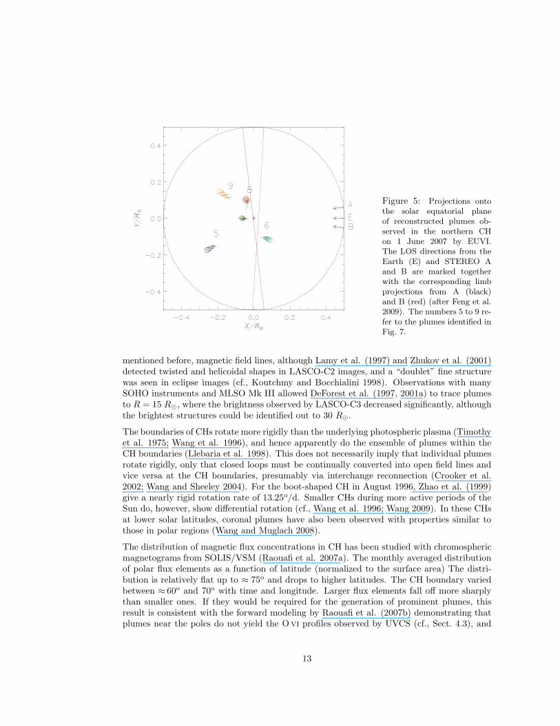
Figure 5: Projections ontothe solar equatorial planeof reconstructed plumes ob-served in the northern CHon 1 June 2007 by EUVI.The LOS directions from theEarth (E) and STEREO Aand B are marked togetherwith the corresponding limbprojections from A (black)and B (red) (after Feng et al.2009). The numbers 5 to 9 re-fer to the plumes identified inFig. 7.

mentioned before, magnetic field lines, although Lamy et al. (1997) and Zhukov et al. (2001)detected twisted and helicoidal shapes in LASCO-C2 images, and a “doublet” fine structurewas seen in eclipse images (cf., Koutchmy and Bocchialini 1998). Observations with manySOHO instruments and MLSO Mk III allowed DeForest et al. (1997, 2001a) to trace plumesto R = 15 R⊙, where the brightness observed by LASCO-C3 decreased significantly, althoughthe brightest structures could be identified out to 30 R⊙.

The boundaries of CHs rotate more rigidly than the underlying photospheric plasma (Timothyet al. 1975; Wang et al. 1996), and hence apparently do the ensemble of plumes within theCH boundaries (Llebaria et al. 1998). This does not necessarily imply that individual plumesrotate rigidly, only that closed loops must be continually converted into open field lines andvice versa at the CH boundaries, presumably via interchange reconnection (Crooker et al.2002; Wang and Sheeley 2004). For the boot-shaped CH in August 1996, Zhao et al. (1999)give a nearly rigid rotation rate of 13.25o/d. Smaller CHs during more active periods of theSun do, however, show differential rotation (cf., Wang et al. 1996; Wang 2009). In these CHsat lower solar latitudes, coronal plumes have also been observed with properties similar tothose in polar regions (Wang and Muglach 2008).

The distribution of magnetic flux concentrations in CH has been studied with chromosphericmagnetograms from SOLIS/VSM (Raouafi et al. 2007a). The monthly averaged distributionof polar flux elements as a function of latitude (normalized to the surface area) The distri-bution is relatively flat up to ≈ 75o and drops to higher latitudes. The CH boundary variedbetween ≈ 60o and 70o with time and longitude. Larger flux elements fall off more sharplythan smaller ones. If they would be required for the generation of prominent plumes, thisresult is consistent with the forward modeling by Raouafi et al. (2007b) demonstrating thatplumes near the poles do not yield the Ovi profiles observed by UVCS (cf., Sect. 4.3), and

13

also with Saito’s (1965a) observations that plumes are rooted preferably in a ring at latitudesbetween 70o and 80o.

3.2 Plume geometry and dimensions

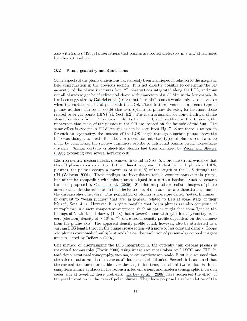
Some aspects of the plume dimensions have already been mentioned in relation to the magneticfield configuration in the previous section. It is not directly possible to determine the 3Dgeometry of the plume structures from 2D observations integrated along the LOS, and thusnot all plumes might be of cylindrical shape with diameters of ≈ 30 Mm in the low corona. Ithas been suggested by Gabriel et al. (2003) that “curtain” plumes would only become visiblewhen the curtain will be aligned with the LOS. These features would be a second type ofplumes as there can be no doubt that near-cylindrical plumes do exist, for instance, thoserelated to bright points (BPs) (cf. Sect. 6.2). The main argument for non-cylindrical plumestructures stems from EIT images in the 17.1 nm band, such as those in Fig. 6, giving theimpression that most of the plumes in the CH are located on the far side of the Sun. Thesame effect is evident in EUVI images as can be seen from Fig. 7. Since there is no reasonfor such an asymmetry, the increase of the LOS length through a curtain plume above thelimb was thought to create the effect. A separation into two types of plumes could also bemade by considering the relative brightness profiles of individual plumes versus heliocentricdistance. Similar curtain- or sheet-like plumes had been identified by Wang and Sheeley(1995) extending over several network cells.

Electron density measurements, discussed in detail in Sect. 5.1, provide strong evidence thatthe CH plasma consists of two distinct density regimes. If identified with plume and IPRplasmas, the plumes occupy a maximum of ≈ 10 % of the length of the LOS through theCH (Wilhelm 2006). These findings are inconsistent with a conterminous curtain plume,but might be compatible with microplumes aligned in a certain fashion. Such a scenariohas been proposed by Gabriel et al. (2009). Simulations produce realistic images of plumeassemblies under the assumption that the footpoints of microplumes are aligned along lanes ofthe chromospheric network. This population of plumes is therefore called “network plumes”in contrast to “beam plumes” that are, in general, related to BPs at some stage of theirlife (cf., Sect. 4.1). However, it is quite possible that beam plumes are also composed ofmicroplumes in a more compact arrangement. Such an option might shed some light on thefindings of Newkirk and Harvey (1968) that a typical plume with cylindrical symmetry has acore (electron) density of ≈ 108 cm−3 and a radial density profile dependent on the distancefrom the plume axis. The apparent density profile could, however, also be attributed to avarying LOS length through the plume cross-section with more or less constant density. Loopsand plumes composed of multiple strands below the resolution of present-day coronal imagersare considered by DeForest (2007).

One method of disentangling the LOS integration in the optically thin coronal plasma isrotational tomography (Frazin 2000) using image sequences taken by LASCO and EIT. Intraditional rotational tomography, two major assumptions are made. First it is assumed thatthe solar rotation rate is the same at all latitudes and altitudes. Second, it is assumed thatthe coronal structures are stable over the acquisition time, i.e. about two weeks. Both as-sumptions induce artifacts in the reconstructed emissions, and modern tomographic inversioncodes aim at avoiding these problems. Barbey et al. (2008) have addressed the effect oftemporal variation in the case of polar plumes. They have proposed a reformulation of the

14

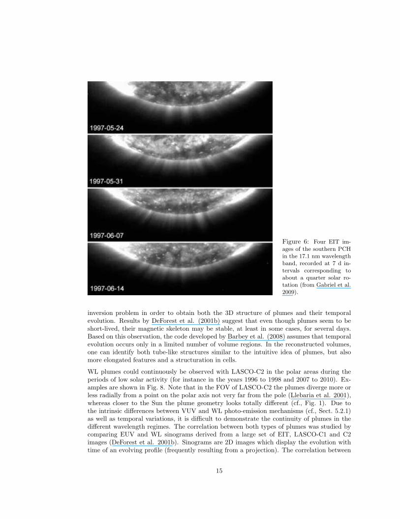
Figure 6: Four EIT im-ages of the southern PCHin the 17.1 nm wavelengthband, recorded at 7 d in-tervals corresponding toabout a quarter solar ro-tation (from Gabriel et al.2009).

inversion problem in order to obtain both the 3D structure of plumes and their temporalevolution. Results by DeForest et al. (2001b) suggest that even though plumes seem to beshort-lived, their magnetic skeleton may be stable, at least in some cases, for several days.Based on this observation, the code developed by Barbey et al. (2008) assumes that temporalevolution occurs only in a limited number of volume regions. In the reconstructed volumes,one can identify both tube-like structures similar to the intuitive idea of plumes, but alsomore elongated features and a structuration in cells.

WL plumes could continuously be observed with LASCO-C2 in the polar areas during theperiods of low solar activity (for instance in the years 1996 to 1998 and 2007 to 2010). Ex-amples are shown in Fig. 8. Note that in the FOV of LASCO-C2 the plumes diverge more orless radially from a point on the polar axis not very far from the pole (Llebaria et al. 2001),whereas closer to the Sun the plume geometry looks totally different (cf., Fig. 1). Due tothe intrinsic differences between VUV and WL photo-emission mechanisms (cf., Sect. 5.2.1)as well as temporal variations, it is difficult to demonstrate the continuity of plumes in thedifferent wavelength regimes. The correlation between both types of plumes was studied bycomparing EUV and WL sinograms derived from a large set of EIT, LASCO-C1 and C2images (DeForest et al. 2001b). Sinograms are 2D images which display the evolution withtime of an evolving profile (frequently resulting from a projection). The correlation between

15

Figure 7: EUVI images in the 17.1 nm band of the northern CH on 1 June 2007 seen from STEREO A(top panel) and B (bottom panel). Strong (beam) plumes are marked by dark dotted lines (afterFeng et al. 2009). The LOS geometries and the reconstructions of the plumes labelled 5 to 9 areshown in Fig. 2. The scales of the axes are in pixels with a size of 1.59′′.

sinograms obtained in different wavelengths and radial distances required an angular correc-tion to compensate for the super-radial expansion. The resulting correlation coefficient wassignificant and established a direct link between EUV and WL plumes. This demonstrationbased on the co-evolution of both features is more robust than image-to-image comparisonsof local details. The CH expansion factor deduced is 2.25 at R = 3 R⊙ in good agreementwith other determinations (DeForest et al. 1997; Cranmer et al. 1999).

With LASCO-C2 it was possible to restitute simultaneously images of the polarized K-coronaand the unpolarized F-corona from polarization measurements (Llebaria et al. 2010). In

16

circular profiles of the K-corona centred on the divergence point, plumes and IPRs appearas random oscillations with a relative amplitude of ≈ 1%. From a spectral analysis of suchoscillations, Llebaria et al. (2002a) concluded that the angular size distribution is fractal,and thus the concept of a characteristic angular size is inapplicable to images of WL plumes.A superposition of multiple strands of different sizes leads to a smooth variation undulatingthe background. The low level of high-frequency oscillations relative to the background isindicative of a large number of tiny plumes along the LOS. Support for this concept has beenobtained by a forward modeling approach (Boursier and Llebaria 2005; cf., Sect. 8.3). Sincethe observed plumes are projections of 3D structures, the fractal 2D structure provides astrong clue for assuming a fractal structure also for the physical plumes, i.e., the 3D electrondensity distribution over the CH domain is probably fractal. Its dimension must be D = 2.9over the CH, in order to obtain a fractal dimension of D = 1.5 in the transverse profile ofWL plumes. The high fractal dimension required by the density distribution of plumes lookssurprising, but is understandable because of the strong integration effect along the LOS. Theimplication that CHs have a fibrous structure might indicate that the beam plumes mentionedearlier should indeed not be thought of as compact entities.

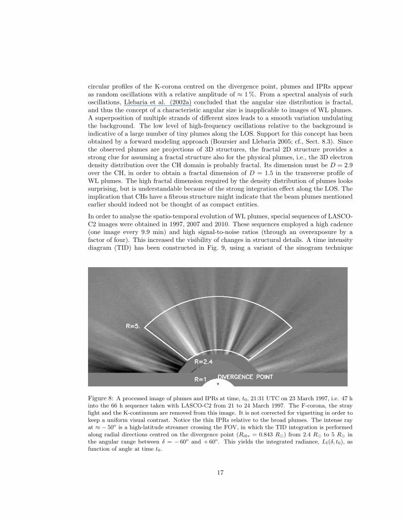
In order to analyse the spatio-temporal evolution of WL plumes, special sequences of LASCO-C2 images were obtained in 1997, 2007 and 2010. These sequences employed a high cadence(one image every 9.9 min) and high signal-to-noise ratios (through an overexposure by afactor of four). This increased the visibility of changes in structural details. A time intensitydiagram (TID) has been constructed in Fig. 9, using a variant of the sinogram technique

Figure 8: A processed image of plumes and IPRs at time, t0, 21:31 UTC on 23 March 1997, i.e. 47 hinto the 66 h sequence taken with LASCO-C2 from 21 to 24 March 1997. The F-corona, the straylight and the K-continuum are removed from this image. It is not corrected for vignetting in order tokeep a uniform visual contrast. Notice the thin IPRs relative to the broad plumes. The intense rayat ≈ − 50o is a high-latitude streamer crossing the FOV, in which the TID integration is performedalong radial directions centred on the divergence point (Rdiv = 0.843 R⊙) from 2.4 R⊙ to 5 R⊙ inthe angular range between δ = − 60o and +60o. This yields the integrated radiance, LI(δ, t0), asfunction of angle at time t0.

17

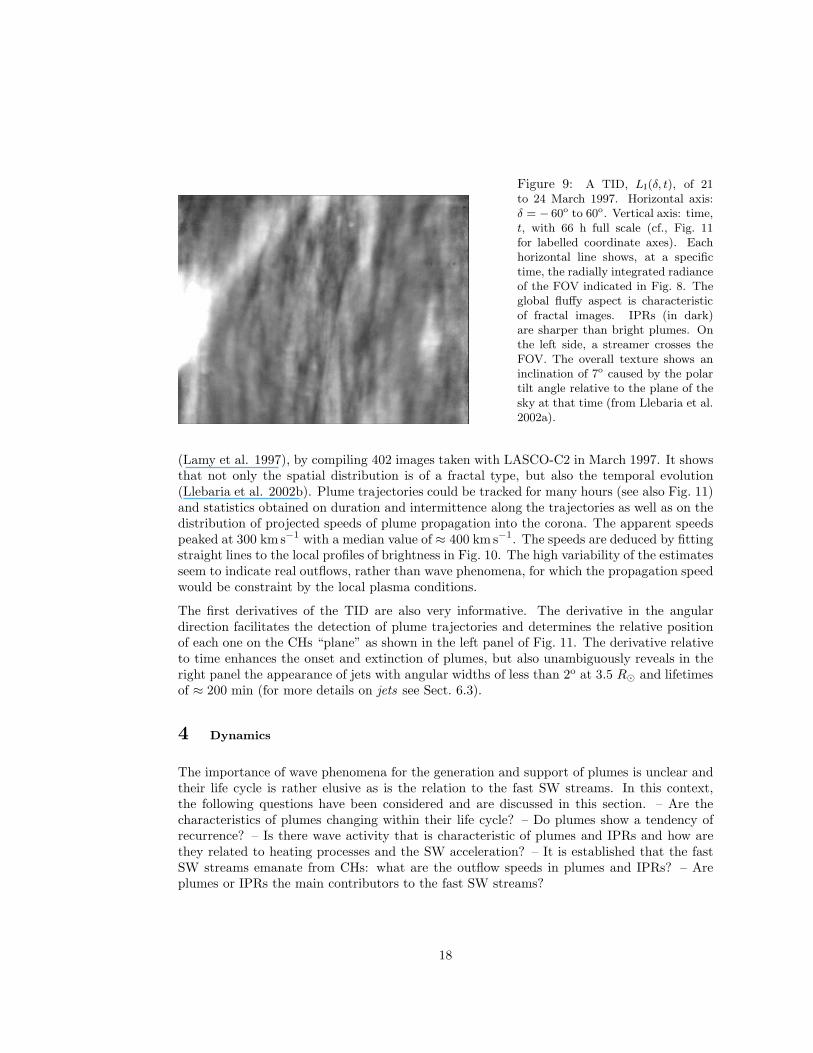
Figure 9: A TID, LI(δ, t), of 21to 24 March 1997. Horizontal axis:δ = − 60o to 60o. Vertical axis: time,t, with 66 h full scale (cf., Fig. 11for labelled coordinate axes). Eachhorizontal line shows, at a specifictime, the radially integrated radianceof the FOV indicated in Fig. 8. Theglobal fluffy aspect is characteristicof fractal images. IPRs (in dark)are sharper than bright plumes. Onthe left side, a streamer crosses theFOV. The overall texture shows aninclination of 7o caused by the polartilt angle relative to the plane of thesky at that time (from Llebaria et al.2002a).

(Lamy et al. 1997), by compiling 402 images taken with LASCO-C2 in March 1997. It showsthat not only the spatial distribution is of a fractal type, but also the temporal evolution(Llebaria et al. 2002b). Plume trajectories could be tracked for many hours (see also Fig. 11)and statistics obtained on duration and intermittence along the trajectories as well as on thedistribution of projected speeds of plume propagation into the corona. The apparent speedspeaked at 300 km s−1 with a median value of ≈ 400 km s−1. The speeds are deduced by fittingstraight lines to the local profiles of brightness in Fig. 10. The high variability of the estimatesseem to indicate real outflows, rather than wave phenomena, for which the propagation speedwould be constraint by the local plasma conditions.

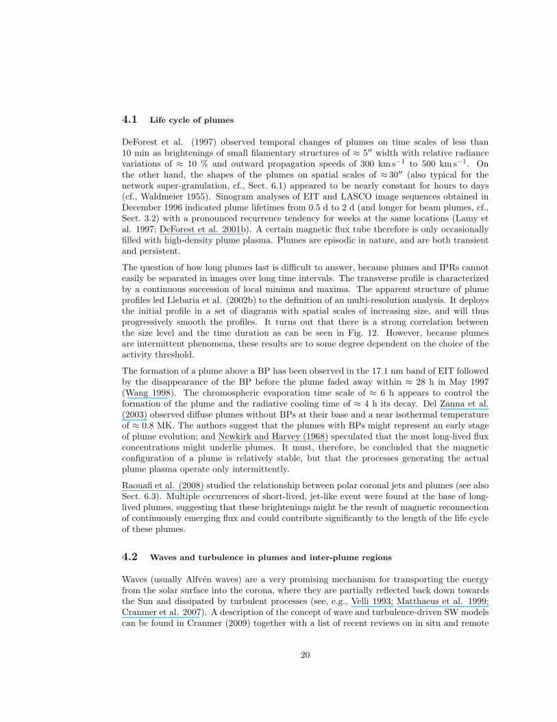
The first derivatives of the TID are also very informative. The derivative in the angulardirection facilitates the detection of plume trajectories and determines the relative positionof each one on the CHs “plane” as shown in the left panel of Fig. 11. The derivative relativeto time enhances the onset and extinction of plumes, but also unambiguously reveals in theright panel the appearance of jets with angular widths of less than 2o at 3.5 R⊙ and lifetimesof ≈ 200 min (for more details on jets see Sect. 6.3).

4 Dynamics

The importance of wave phenomena for the generation and support of plumes is unclear andtheir life cycle is rather elusive as is the relation to the fast SW streams. In this context,the following questions have been considered and are discussed in this section. – Are thecharacteristics of plumes changing within their life cycle? – Do plumes show a tendency ofrecurrence? – Is there wave activity that is characteristic of plumes and IPRs and how arethey related to heating processes and the SW acceleration? – It is established that the fastSW streams emanate from CHs: what are the outflow speeds in plumes and IPRs? – Areplumes or IPRs the main contributors to the fast SW streams?

18

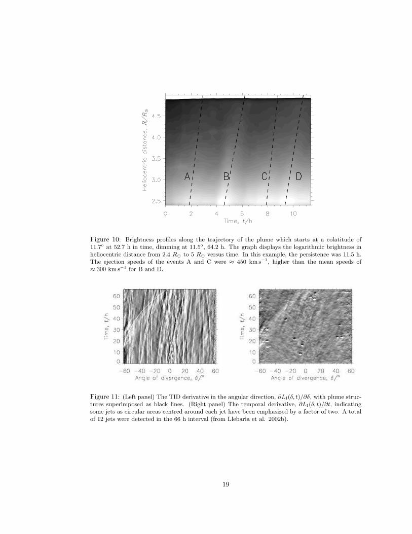
Figure 10: Brightness profiles along the trajectory of the plume which starts at a colatitude of11.7o at 52.7 h in time, dimming at 11.5o, 64.2 h. The graph displays the logarithmic brightness inheliocentric distance from 2.4 R⊙ to 5 R⊙ versus time. In this example, the persistence was 11.5 h.The ejection speeds of the events A and C were ≈ 450 kms−1, higher than the mean speeds of≈ 300 kms−1 for B and D.

Figure 11: (Left panel) The TID derivative in the angular direction, ∂LI(δ, t)/∂δ, with plume struc-tures superimposed as black lines. (Right panel) The temporal derivative, ∂LI(δ, t)/∂t, indicatingsome jets as circular areas centred around each jet have been emphasized by a factor of two. A totalof 12 jets were detected in the 66 h interval (from Llebaria et al. 2002b).

19

4.1 Life cycle of plumes

DeForest et al. (1997) observed temporal changes of plumes on time scales of less than10 min as brightenings of small filamentary structures of ≈ 5′′ width with relative radiancevariations of ≈ 10 % and outward propagation speeds of 300 kms−1 to 500 km s−1. Onthe other hand, the shapes of the plumes on spatial scales of ≈ 30′′ (also typical for thenetwork super-granulation, cf., Sect. 6.1) appeared to be nearly constant for hours to days(cf., Waldmeier 1955). Sinogram analyses of EIT and LASCO image sequences obtained inDecember 1996 indicated plume lifetimes from 0.5 d to 2 d (and longer for beam plumes, cf.,Sect. 3.2) with a pronounced recurrence tendency for weeks at the same locations (Lamy etal. 1997; DeForest et al. 2001b). A certain magnetic flux tube therefore is only occasionallyfilled with high-density plume plasma. Plumes are episodic in nature, and are both transientand persistent.

The question of how long plumes last is difficult to answer, because plumes and IPRs cannoteasily be separated in images over long time intervals. The transverse profile is characterizedby a continuous succession of local minima and maxima. The apparent structure of plumeprofiles led Llebaria et al. (2002b) to the definition of an multi-resolution analysis. It deploysthe initial profile in a set of diagrams with spatial scales of increasing size, and will thusprogressively smooth the profiles. It turns out that there is a strong correlation betweenthe size level and the time duration as can be seen in Fig. 12. However, because plumesare intermittent phenomena, these results are to some degree dependent on the choice of theactivity threshold.

The formation of a plume above a BP has been observed in the 17.1 nm band of EIT followedby the disappearance of the BP before the plume faded away within ≈ 28 h in May 1997(Wang 1998). The chromospheric evaporation time scale of ≈ 6 h appears to control theformation of the plume and the radiative cooling time of ≈ 4 h its decay. Del Zanna et al.(2003) observed diffuse plumes without BPs at their base and a near isothermal temperatureof ≈ 0.8 MK. The authors suggest that the plumes with BPs might represent an early stageof plume evolution; and Newkirk and Harvey (1968) speculated that the most long-lived fluxconcentrations might underlie plumes. It must, therefore, be concluded that the magneticconfiguration of a plume is relatively stable, but that the processes generating the actualplume plasma operate only intermittently.

Raouafi et al. (2008) studied the relationship between polar coronal jets and plumes (see alsoSect. 6.3). Multiple occurrences of short-lived, jet-like event were found at the base of long-lived plumes, suggesting that these brightenings might be the result of magnetic reconnectionof continuously emerging flux and could contribute significantly to the length of the life cycleof these plumes.

4.2 Waves and turbulence in plumes and inter-plume regions

Waves (usually Alfven waves) are a very promising mechanism for transporting the energyfrom the solar surface into the corona, where they are partially reflected back down towardsthe Sun and dissipated by turbulent processes (see, e.g., Velli 1993; Matthaeus et al. 1999;Cranmer et al. 2007). A description of the concept of wave and turbulence-driven SW modelscan be found in Cranmer (2009) together with a list of recent reviews on in situ and remote

20

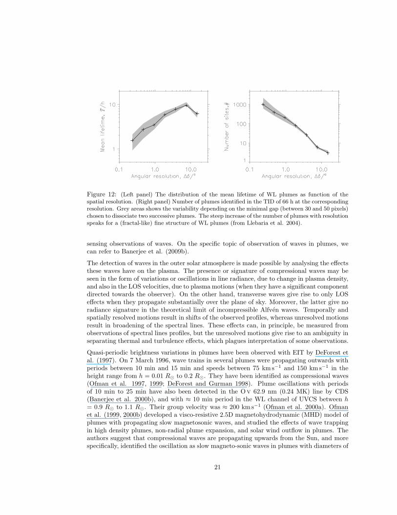
Figure 12: (Left panel) The distribution of the mean lifetime of WL plumes as function of thespatial resolution. (Right panel) Number of plumes identified in the TID of 66 h at the correspondingresolution. Grey areas shows the variability depending on the minimal gap (between 30 and 50 pixels)chosen to dissociate two successive plumes. The steep increase of the number of plumes with resolutionspeaks for a (fractal-like) fine structure of WL plumes (from Llebaria et al. 2004).

sensing observations of waves. On the specific topic of observation of waves in plumes, wecan refer to Banerjee et al. (2009b).

The detection of waves in the outer solar atmosphere is made possible by analysing the effectsthese waves have on the plasma. The presence or signature of compressional waves may beseen in the form of variations or oscillations in line radiance, due to change in plasma density,and also in the LOS velocities, due to plasma motions (when they have a significant componentdirected towards the observer). On the other hand, transverse waves give rise to only LOSeffects when they propagate substantially over the plane of sky. Moreover, the latter give noradiance signature in the theoretical limit of incompressible Alfven waves. Temporally andspatially resolved motions result in shifts of the observed profiles, whereas unresolved motionsresult in broadening of the spectral lines. These effects can, in principle, be measured fromobservations of spectral lines profiles, but the unresolved motions give rise to an ambiguity inseparating thermal and turbulence effects, which plagues interpretation of some observations.

Quasi-periodic brightness variations in plumes have been observed with EIT by DeForest etal. (1997). On 7 March 1996, wave trains in several plumes were propagating outwards withperiods between 10 min and 15 min and speeds between 75 km s−1 and 150 kms−1 in theheight range from h = 0.01 R⊙ to 0.2 R⊙. They have been identified as compressional waves(Ofman et al. 1997, 1999; DeForest and Gurman 1998). Plume oscillations with periodsof 10 min to 25 min have also been detected in the Ov 62.9 nm (0.24 MK) line by CDS(Banerjee et al. 2000b), and with ≈ 10 min period in the WL channel of UVCS between h= 0.9 R⊙ to 1.1 R⊙. Their group velocity was ≈ 200 kms−1 (Ofman et al. 2000a). Ofmanet al. (1999, 2000b) developed a visco-resistive 2.5D magnetohydrodynamic (MHD) model ofplumes with propagating slow magnetosonic waves, and studied the effects of wave trappingin high density plumes, non-radial plume expansion, and solar wind outflow in plumes. Theauthors suggest that compressional waves are propagating upwards from the Sun, and morespecifically, identified the oscillation as slow magneto-sonic waves in plumes with diameters of

21

≈ 30 Mm. On the other hand, these time scales are commensurate with the slow photosphericmotions thought to drive Alfvenic (incompressible) fluctuations that propagate upwards andare implicated in heating at coronal altitudes (see, e.g., Dmitruk et al. 2002; Verdini et al.2010). Consequently, it is not out of the question that plume formation and dynamics is insome way related to this broader issue. Very long-period activity (≈ 170 min) in a PCH hasbeen reported by Popescu et al. (2005). In a review article, Ofman (2005) concluded thatthe energy flux in slow-mode waves is too small for all of the coronal heating and that othermodes must be considered in addition.

Above BP groups, torsional Alfvenic perturbations have been detected through non-thermalbroadenings of the Hα line profile (Jess et al. 2009). The authors conclude that the energyflux of these waves is sufficient to heat the corona. Indirect evidence for Alfven waves hasbeen found in CHs by Banerjee et al. (1998, 2009a) as well as by Dolla and Solomon (2008)from measurements of line broadenings in spectra obtained with very long exposure times.The propagation and dissipation of Alfven waves in plumes were discussed by Ofman andDavila (1995) using a 2.5D MHD model. The injection of Alfven waves and the formation ofa jet was recently studied by Pinto et al. (2010) using such a model.

Recently, Gupta et al. (2010) detected the presence of propagating waves in an IPR with a15 min to 20 min periodicity—obtained from a wavelet analysis—and a propagation speed in-creasing from (130 ± 14) kms−1 just above the limb to (330 ± 140) km s−1 around 160′′ abovethe limb. The distant-time map of the Fexii radiance over nearly 2 h is shown in the upperpanel of Fig. 13. Although the waves are best seen in radiance, significant power at thoseperiodicities is also detected in both Doppler width and shift. In the adjacent plume re-gion (lower panel), propagating radiance disturbances also appear to be present (no spectralprofiles are available) with the same range of periodicity, but with propagation speeds in therange of (135 ± 18) kms−1 to (165 ± 43) kms−1. The plume observations might, however, beaffected by the IPRs along the LOS, because of the low electron temperature in plumes, thehigh formation temperature of the Fexii line (cf., Figs. 18 and 19) and the more favourableconditions for such emissions in IPRs. Based on the acceleration to supersonic speeds and thesignature in Doppler width and shift, the authors suggest that in IPRs the waves are likelyeither Alfvenic or fast magneto-acoustic, whereas they are slow magneto-acoustic in plumes.

An important feature of turbulence models (Dmitruk et al. 2001) is the non-linear pump-ing of non-propagating ”zero frequency” structures. These would appear in observations asstrong transverse gradients. When present these ”quasi-2D” fluctuations can catalyse a pow-erful cascade perpendicular to the large-scale magnetic field that may drive strong turbulentheating at fine transverse scales (e.g., Verdini et al. 2010). For this reason in consideringturbulence models, it is essential to examine fluctuations that may not be described by anylinear wave mode (see, e.g., Dmitruk and Matthaeus 2009). It is possible that plumes, withtheir characteristic transverse structure, may participate in these low-frequency dynamicalcouplings, and thus could play a direct role in coronal turbulence.

4.3 Outflows in plumes, inter-plume regions and coronal holes

Coronal plumes together with other dynamic structures in the solar atmosphere, such asspicules, macrospicules and chromospheric jets, are potential sources of the SW. The contri-bution of plumes to the fast SW has been disputed in the literature. Some studies indicate

22

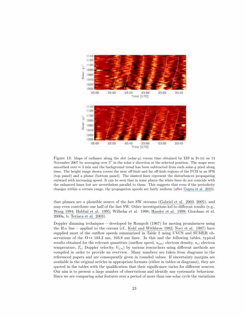
Figure 13: Maps of radiance along the slot (solar-y) versus time obtained by EIS in Fexii on 13November 2007 by averaging over 5′′ in the solar-x direction at the selected position. The maps weresmoothed over ≈ 3 min and the background trend has been subtracted from each solar-y pixel alongtime. The height range shown covers the near off-limb and far off-limb regions of the PCH in an IPR(top panel) and a plume (bottom panel). The slanted lines represent the disturbances propagatingoutward with increasing speed. It can be seen that in some places the white lines do not coincide withthe enhanced lanes but are nevertheless parallel to them. This suggests that even if the periodicitychanges within a certain range, the propagation speeds are fairly uniform (after Gupta et al. 2010).

that plumes are a plausible source of the fast SW streams (Gabriel et al. 2003, 2005), andmay even contribute one half of the fast SW. Other investigations led to different results (e.g.,Wang 1994; Habbal et al. 1995; Wilhelm et al. 1998; Hassler et al. 1999; Giordano et al.2000a, b; Teriaca et al. 2003).

Doppler dimming techniques—developed by Rompolt (1967) for moving prominences usingthe Hα line—applied to the corona (cf., Kohl and Withbroe 1982; Noci et al. 1987) havesupplied most of the outflow speeds summarized in Table 2 using UVCS and SUMER ob-servations of the Ovi 103.2 nm, 103.8 nm lines. In this and the following tables, typicalresults obtained for the relevant quantities (outflow speed, uout; electron density, ne; electrontemperature, Te; Doppler velocity, V1/e) by various researchers using different methods arecompiled in order to provide an overview. Many numbers are taken from diagrams in thereferenced papers and are consequently given in rounded values. If uncertainty margins areavailable in the original articles in appropriate formats (either in tables or diagrams), they arequoted in the tables with the qualification that their significance varies for different sources.Our aim is to present a large number of observations and identify any systematic behaviour.Since we are comparing solar features over a period of more than one solar cycle the variations

23

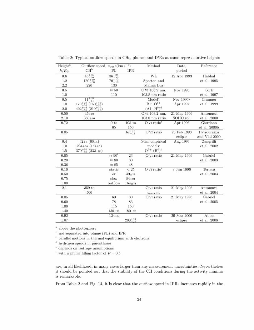
Table 2: Typical outflow speeds in CHs, plumes and IPRs at some representative heights

Heighta Outflow speed, uout/(km s−1) Method Date, Reference

h/R⊙ CHb PL IPR period

0.6 45+55−20 36+25

−20 WL 12 Apr 1993 Habbal1.2 130+50

−60 70+70−10 Spartan and et al. 1995

2.2 220 130 Mauna Loa

0.5 ≈ 50 Ovi 103.2 nm, Nov 1996 Corti1.0 110 103.8 nm ratio et al. 1997

0.5 11+38−11 Modelc Nov 1996/ Cranmer

1.0 179+78−76 (150+49

−55) B1: O5+ Apr 1997 et al. 1999

2.0 402+44−68 (219+30

−23) (A1: H0)d

0.50 45±10 Ovi 103.2 nm, 21 May 1996 Antonucci2.10 360±40 103.8 nm ratio SOHO roll et al. 2000

0.72 0 to 105 to Ovi ratioe Apr 1996 Giordano65 150 et al. 2000b

0.05 67+16−14 Ovi ratio 26 Feb 1998 Patsourakos

eclipse and Vial 2000

0.4 62±5 (60±5) Semi-empirical Aug 1996 Zangrilli1.0 234±20 (154±5) models: et al. 20021.5 370+60

−90 (232±30) O5+ (H0)d

0.05 ≈ 90f 23 Ovi ratio 21 May 1996 Gabriel0.20 ≈ 80 30 et al. 20030.36 ≈ 85 48

0.10 static < 25 Ovi ratioe 3 Jun 1996 Teriaca0.50 or 49±28 et al. 20030.75 slow 84±21

1.00 outflow 164±38

2.1 359 to Ovi ratio 21 May 1996 Antonucci500 uout, ne et al. 2004

0.05 60 30 Ovi ratio 21 May 1996 Gabriel0.60 78 83 et al. 20051.00 115 1501.40 130±20 180±20

0.92 124±5 Ovi ratio 29 Mar 2006 Abbo1.07 208+41

−27 eclipse et al. 2008

a above the photosphereb not separated into plume (PL) and IPRc parallel motions in thermal equilibrium with electronsd hydrogen speeds in parenthesese depends on isotropy assumptionsf with a plume filling factor of F = 0.5

are, in all likelihood, in many cases larger than any measurement uncertainties. Neverthelessit should be pointed out that the stability of the CH conditions during the activity minimais remarkable.

From Table 2 and Fig. 14, it is clear that the outflow speed in IPRs increases rapidly in the

24

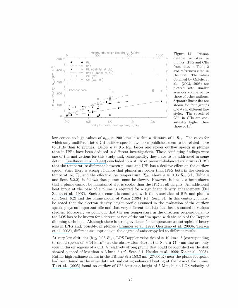
Figure 14: Plasmaoutflow velocities inplumes, IPRs and CHsfrom data in Table 2and references cited inthe text. The valuesobtained by Gabriel etal. (2003, 2005) areplotted with smallersymbols compared tothose of other authors.Separate linear fits areshown for four groupsof data in different linestyles. The speeds ofO5+ in CHs are con-sistently higher thanthose of H0.

low corona to high values of uout ≈ 200 km s−1 within a distance of 1 R⊙. The cases forwhich only undifferentiated CH outflow speeds have been published seem to be related moreto IPRs than to plumes. Below h ≈ 0.5 R⊙, faster and slower outflow speeds in plumesthan in IPRs have been deduced in different investigations. These conflicting findings wereone of the motivations for this study and, consequently, they have to be addressed in somedetail. Casalbuoni et al. (1999) concluded in a study of pressure-balanced structures (PBS)that the temperature difference between plumes and IPR has a decisive effect on the outflowspeed. Since there is strong evidence that plumes are cooler than IPRs both in the electrontemperature, Te, and the effective ion temperature, Teff , above h ≈ 0.03 R⊙ (cf., Table 4and Sect. 5.2.2), it follows that plumes must be slower. However, it has also been shownthat a plume cannot be maintained if it is cooler than the IPR at all heights. An additionalheat input at the base of a plume is required for a significant density enhancement (DelZanna et al. 1997). Such a scenario is consistent with the association of BPs and plumes(cf., Sect. 6.2) and the plume model of Wang (1994) (cf., Sect. 8). In this context, it mustbe noted that the electron density height profile assumed in the evaluation of the outflowspeeds plays an important role and that very different densities had been assumed in variousstudies. Moreover, we point out that the ion temperature in the direction perpendicular tothe LOS has to be known for a determination of the outflow speed with the help of the Dopperdimming technique. Although there is strong evidence for temperature anisotropies of heavyions in IPRs and, possibly, in plumes (Cranmer et al. 1999; Giordano et al. 2000b; Teriacaet al. 2003), different assumptions on the degree of anisotropy led to different results.

At very low altitudes (h ≤ 0.03 R⊙), LOS Doppler velocities of ≈ 10 km s−1 (correspondingto radial speeds of ≈ 14 km s−1 at the observation site) in the Neviii 77.0 nm line are onlyseen in darker regions of a CH. A relatively strong plume that could be identified on the diskshowed a speed of less than ≈ 3 km s−1 (cf., Sect. 3.1; Hassler et al. 1999; Xia et al. 2003).Rather high radiance values in the TR line Si ii 153.3 nm (27 000 K) near the plume footpointhad been found in the same data set, indicating enhanced heating at the base of the plume.Tu et al. (2005) found no outflow of C3+ ions at a height of 5 Mm, but a LOS velocity of

25

≈ 10 kms−1 in funnels of the same CH at 20 Mm (for Ne7+). However, no significant outflowcould be detected in a magnetic plume structure (cf., Sect. 3.1). It thus appears as if, indeed,the IPRs have larger outflow speeds along a height profile and, together with the small fillingfactor of plumes in CHs, provide the main contribution to the fast SW streams as suggestedby Wang (1994). The funnels harbouring the outflows seen in Neviii are most likely rootedin flux concentrations described by Tsuneta et al. (2008b). The picture of expanding coronalfunnels is supported by the findings of Tian et al. (2010) that increasingly larger patchesof blue-shifted line profiles (outflows) are observed in hotter spectral lines with EIS in theon-disk part of a PCH.

Raouafi et al. (2007b) studied the plasma dynamics (outflow speed and turbulence) in-side coronal polar plumes and compared line profiles (mainly of Ovi) observed by UVCS atthe minimum between solar cycles 22 and 23 with model calculations. Maxwellian velocitydistributions with different widths are assumed for both plumes and IPRs, and different com-binations of the outflow velocities, uout, and most-probable speeds, V1/e (cf., Sect. 5.2.2) areconsidered. The observed profiles are reproduced best by low outflow speeds close to the Sunin plumes that increased with height to reach IPR values above h ≈ 3 R⊙. The most-probablespeeds in plumes and IPRs assumed are included in Table 5.

In equatorial coronal holes (ECH), with characteristics very similar to PCHs, outflows alongopen field lines can be detected in spectral lines with formation temperatures above 0.1 MK(cf., Sect. 5.2.1). An average outflow speed of uout ≈ 5 km s−1 was measured for Ne7+ ionsand of ≈ 10 km s−1 for Mg8+ (Wilhelm et al. 2002a; Xia et al. 2004; Wiegelmann et al.2005). Woo (2007) summarized outflow observations as filamentary structures on open fieldlines within the so-called closed corona.

On balance, there seems to be some evidence that IPR outflow speeds become significantlygreater than outflows in plumes at increasing altitude in the lower corona. In this context,Sheeley et al. (1997) made an interesting remark on the direction of time that can always beidentified in coronal streamers, but not in polar coronal plumes— implying that the outflowsignatures in plumes are less pronounced.

5 Plasma conditions in coronal holes

The knowledge of the plasma conditions in plumes and their environment in CHs is critical foran understanding of the plume physics. We asked questions as follows: – Can standard heightprofiles of the electron density in plumes and IPRs be defined considering that the measure-ments obtained with various methods agree remarkably well within the general variability ofsolar features? – Specifically, what is the plume/IPR density ratio and its potential variationwith height? – What are the plume and IPR electron and ion temperatures as a functionof height? – Is there a significant anisotropy of the ion temperatures in plumes and IPRs?– What can be said about the elemental abundance in plumes and IPRs, and, specifically,about the first-ionization potential (FIP) effect? – What is the expected FIP and ionizationstate signature of plumes in the SW, given a hypothesis for their source? – Is it agreed thatthere are different plasma regimes present along the LOS in CH observations—plumes andIPRs?

A brief discussion of the resulting plasma pressures is included in Sect. 6.4.

26

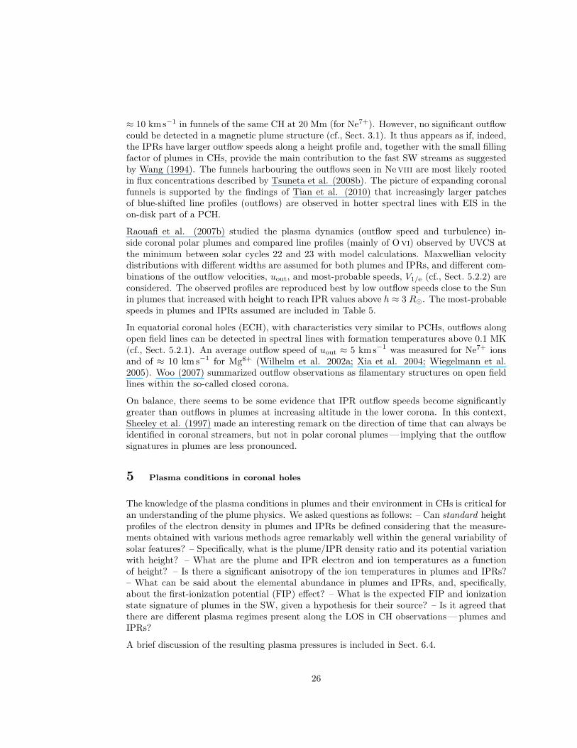
Figure 15: (a) Radianceof the Siviii 144.6 nm linein the southern CH be-fore and after the totaleclipse on 29 March 2006.During the actual eclipse,the scan was interruptedin favour of high-cadenceOvi observations, an ex-ample of which is shownin Fig. 26. The concen-tric height ranges, h1 toh7, outline the data se-lection in Fig. 16b. Ra-dius vectors at ± 12o areindicated. (b) Electrondensity determined fromthe LOS Siviii line ratioL144.6/L144.0 . The pro-jection of a plume nearx = 200′′ is shown for acomparison with the ra-dius vector in panel (a).

5.1 Electron densities in plumes and inter-plume regions

Above the solar limb, coronal plumes seen in WL appear brighter than the surroundingmedium which led many authors to the conclusion that they are denser than the backgroundcorona (called here IPR) (van de Hulst 1950b; Saito 1965a; Koutchmy 1977; Ahmad andWithbroe 1977; Fisher and Guhathakurta 1995). The density measurements in WL utilizethe fact that Thomson scattering of electrons produces polarized light, whereas the muchstronger F-coronal radiance from dust particles is unpolarized. The polarized brightness

pB =√

Q2 + U2 , (1)

with Q and U the relevant Stokes parameters, then has to be related to the electron densityalong the LOS taking into account the dependence of pB upon the distance from the planeof the sky (cf., Koutchmy and Bocchialini 1998).

VUV observations rely on atomic data for a determination of the electron density from line-ratio measurements. In the polar corona the nitrogen-like ion Si7+ and its magnetic dipoletransitions 2s22p3 4S3/2−2s22p3 2D3/2 and 2s22p3 4S3/2−2s22p3 2D5/2 with the correspondingemission lines Siviii 144.6 nm and 144.0 nm provide a convenient means of deducing ne

through the radiance ratio RSi = L144.6/L144.0. It is density sensitive, because de-excitationof the D5/2 level occurs not only radiatively, but also collisionally (see Laming et al. 1997;Doschek et al. 1997 for a conversion procedure). Compared with this procedure, the electrondensities determined from RSi with the help of the CHIANTI atomic data base yield slightlyhigher values (Banerjee et al. 1998). Warren and Hassler (1999) discussed, in addition, otherdensity-sensitive line ratios, and derived CH densities that are in good agreement with the

27

Siviii values. In an ECH, Del Zanna and Bromage (1999) measured coronal electron densitiesof ne ≈ 3× 108 cm−2 (approximately a factor of two lower than in the adjoining QS regions).A selection of typical electron density measurements, obtained with the help of spacecraft andeclipse observations, is compiled in Table 3 for some representative heliocentric distances.

For an isothermal plasma, optically thin for a certain emission line, the LOS-integrated elec-tron density (along the z direction) can be deduced from

∫

n2e dz, the emission measure (EM)

(see, e.g., Raymond and Doyle 1981), which in turn can be obtained from radiance observa-tion, if the electron temperature and the element abundance are known (cf. Sects. 5.2.1 and5.3). It is important to note that the Thomson scattering depends linearly on the electrondensity, whereas the emission process is a function of n2

e . So that WL observations yieldthe mean value of the electron density, 〈ne〉, whereas spectroscopic line ratios yield

√

〈n2e〉.

These will not be the same where there are inhomogeneities in the plasma, and there is someevidence for this. Such inhomegeneities could have different scales, for example beam plumesand IPRs, network plumes, or even much finer structures due to turbulence.

A radiance map of the southern low corona in the Siviii 144.6 nm line during the eclipsecampaign 2006 is shown in Fig. 15a together with the electron densities in panel (b), derivedfrom the L144.6/L144.0 photon radiance ratio observed in 96 raster steps of the SUMER slitfrom W to E. The height resolution is limited by the count statistics to a super-pixel of eightdetector pixels. Several plume signatures with enhanced density can be identified. The line-ratio method—as applied here so far—obviously suffers from LOS effects if there are density(and temperature) variations along the integration path, complications discussed by Habbalet al. (1993). The polarization brightness, on the other hand, depends more on the conditionsnear the plane of the sky (Munro and Jackson 1977; Koutchmy and Bocchialini 1998), so thatplumes and IPRs can probably be separated more effectively. From an analysis of the polarizedK-corona measurements obtained with the EKPol polarimeter, electron density profiles havebeen derived in plume and IPR structures for the total eclipse on 29 March 2006 (Abbo etal. 2008; see Table 3 for representative values).

In an attempt to improve the separation of plume and IPR plasma regimes with the help ofline-ratio observations, the radiances L144.6 and L144.0 measured with SUMER on 29 March2006 are plotted in Fig. 16(a) and (b) averaged over certain height intervals per W-E step. Inthe upper panel, linear fits are calculated from data points obtained along tangential heightranges following a procedure developed earlier for 2005 observations (Wilhelm 2006). Inthe lower panel, the same measurements are organized according to concentric height rangesdefined in Fig. 15. The highest range, h7, has been omitted, because the data were too noisy.In both plots, the extrapolations of the linear fits do not pass through the origins of thediagrams as indicated for the lowest heights, h1 and h2 in panel (a). The only explanationfor this behaviour appears to be that more than one density regime is encountered at most ofthe LOS directions. Under the assumption that the lowest radiances observed for each heightrange— encircled in panel (b)—represent pure IPR plasma (or at least the best estimatewe can get), the ratio of these radiances then provides the density of the IPR plasma.7 Thehighly significant regression lines allow us to conclude that there must be (at a given height)another plasma with a rather well-defined higher density as determined from the slopes. Avarying amount of this “plume” plasma is sampled at different LOS positions. The variations

7This method has some similarities with the radial background subtraction employed by DeForest andGurman (1998).

28

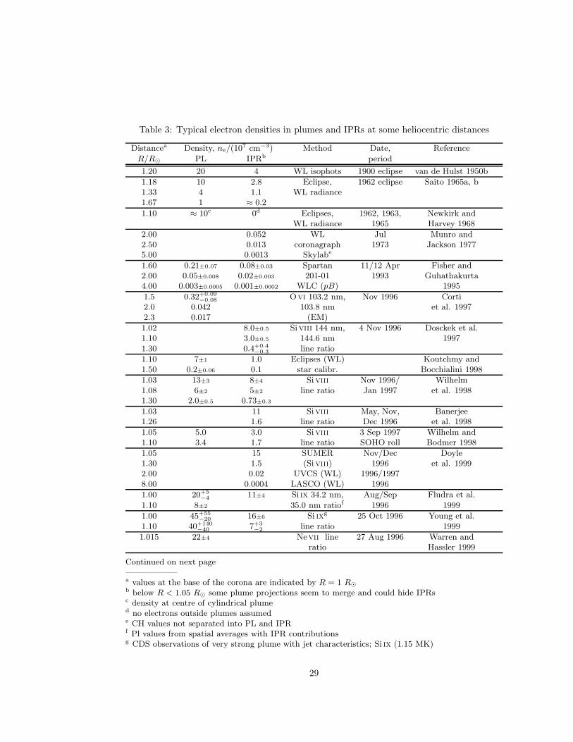
Table 3: Typical electron densities in plumes and IPRs at some heliocentric distances

Distancea Density, ne/(107 cm−3) Method Date, Reference

R/R⊙ PL IPRb period

1.20 20 4 WL isophots 1900 eclipse van de Hulst 1950b

1.18 10 2.8 Eclipse, 1962 eclipse Saito 1965a, b1.33 4 1.1 WL radiance1.67 1 ≈ 0.2

1.10 ≈ 10c 0d Eclipses, 1962, 1963, Newkirk andWL radiance 1965 Harvey 1968

2.00 0.052 WL Jul Munro and2.50 0.013 coronagraph 1973 Jackson 19775.00 0.0013 Skylabe

1.60 0.21±0.07 0.08±0.03 Spartan 11/12 Apr Fisher and2.00 0.05±0.008 0.02±0.003 201-01 1993 Guhathakurta4.00 0.003±0.0005 0.001±0.0002 WLC (pB) 1995

1.5 0.32+0.09−0.08 Ovi 103.2 nm, Nov 1996 Corti

2.0 0.042 103.8 nm et al. 19972.3 0.017 (EM)

1.02 8.0±0.5 Siviii 144 nm, 4 Nov 1996 Dosckek et al.1.10 3.0±0.5 144.6 nm 19971.30 0.4+0.4

−0.3 line ratio

1.10 7±1 1.0 Eclipses (WL) Koutchmy and1.50 0.2±0.06 0.1 star calibr. Bocchialini 1998

1.03 13±3 8±4 Siviii Nov 1996/ Wilhelm1.08 6±2 5±2 line ratio Jan 1997 et al. 19981.30 2.0±0.5 0.73±0.3

1.03 11 Siviii May, Nov, Banerjee1.26 1.6 line ratio Dec 1996 et al. 1998

1.05 5.0 3.0 Siviii 3 Sep 1997 Wilhelm and1.10 3.4 1.7 line ratio SOHO roll Bodmer 1998

1.05 15 SUMER Nov/Dec Doyle1.30 1.5 (Siviii) 1996 et al. 19992.00 0.02 UVCS (WL) 1996/19978.00 0.0004 LASCO (WL) 1996

1.00 20+5−4 11±4 Si ix 34.2 nm, Aug/Sep Fludra et al.

1.10 8±2 35.0 nm ratiof 1996 1999

1.00 45+55−20 16±6 Si ixg 25 Oct 1996 Young et al.

1.10 40+140−40 7+3

−2 line ratio 1999

1.015 22±4 Nevii line 27 Aug 1996 Warren andratio Hassler 1999

Continued on next page——————a values at the base of the corona are indicated by R = 1 R⊙b below R < 1.05 R⊙ some plume projections seem to merge and could hide IPRsc density at centre of cylindrical plumed no electrons outside plumes assumede CH values not separated into PL and IPRf Pl values from spatial averages with IPR contributionsg CDS observations of very strong plume with jet characteristics; Si ix (1.15 MK)

29

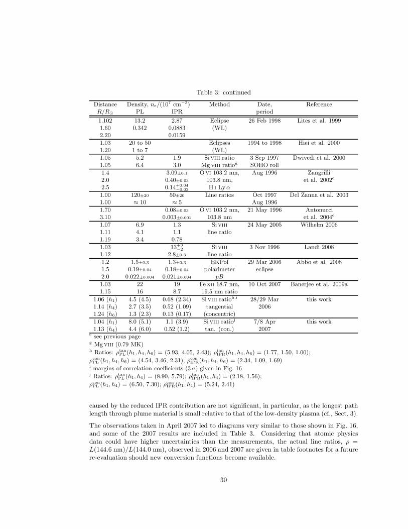
Table 3: continued

Distance Density, ne/(107 cm−3) Method Date, Reference

R/R⊙ PL IPR period

1.102 13.2 2.87 Eclipse 26 Feb 1998 Lites et al. 19991.60 0.342 0.0883 (WL)2.20 0.0159

1.03 20 to 50 Eclipses 1994 to 1998 Hiei et al. 20001.20 1 to 7 (WL)

1.05 5.2 1.9 Siviii ratio 3 Sep 1997 Dwivedi et al. 20001.05 6.4 3.0 Mgviii ratiog SOHO roll

1.4 3.09±0.1 Ovi 103.2 nm, Aug 1996 Zangrilli2.0 0.40±0.03 103.8 nm, et al. 2002e

2.5 0.14+0.04−0.03 H i Lyα

1.00 120±20 50±20 Line ratios Oct 1997 Del Zanna et al. 20031.00 ≈ 10 ≈ 5 Aug 1996

1.70 0.08±0.03 Ovi 103.2 nm, 21 May 1996 Antonucci3.10 0.003±0.001 103.8 nm et al. 2004e

1.07 6.9 1.3 Siviii 24 May 2005 Wilhelm 20061.11 4.1 1.1 line ratio1.19 3.4 0.78

1.03 13+3−2 Siviii 3 Nov 1996 Landi 2008

1.12 2.8±0.3 line ratio

1.2 1.5±0.3 1.3±0.3 EKPol 29 Mar 2006 Abbo et al. 20081.5 0.19±0.04 0.18±0.04 polarimeter eclipse2.0 0.022±0.004 0.021±0.004 pB

1.03 22 19 Fexii 18.7 nm, 10 Oct 2007 Banerjee et al. 2009a1.15 16 8.7 19.5 nm ratio

1.06 (h1) 4.5 (4.5) 0.68 (2.34) Siviii ratioh,i 28/29 Mar this work1.14 (h4) 2.7 (3.5) 0.52 (1.09) tangential 20061.24 (h6) 1.3 (2.3) 0.13 (0.17) (concentric)

1.04 (h1) 8.0 (5.1) 1.1 (3.9) Siviii ratioj 7/8 Apr this work1.13 (h4) 4.4 (6.0) 0.52 (1.2) tan. (con.) 2007

e see previous pageg Mgviii (0.79 MK)h Ratios: ρtanPL (h1, h4, h6) = (5.93, 4.05, 2.43); ρtanIPR(h1, h4, h6) = (1.77, 1.50, 1.00);

ρconPL (h1, h4, h6) = (4.54, 3.46, 2.31); ρconIPR(h1, h4, h6) = (2.34, 1.09, 1.69)i margins of correlation coefficients (3σ) given in Fig. 16j Ratios: ρtanPL (h1, h4) = (8.90, 5.79); ρtanIPR(h1, h4) = (2.18, 1.56);

ρconPL (h1, h4) = (6.50, 7.30); ρconIPR(h1, h4) = (5.24, 2.41)

caused by the reduced IPR contribution are not significant, in particular, as the longest pathlength through plume material is small relative to that of the low-density plasma (cf., Sect. 3).

The observations taken in April 2007 led to diagrams very similar to those shown in Fig. 16,and some of the 2007 results are included in Table 3. Considering that atomic physicsdata could have higher uncertainties than the measurements, the actual line ratios, ρ =L(144.6 nm)/L(144.0 nm), observed in 2006 and 2007 are given in table footnotes for a futurere-evaluation should new conversion functions become available.

30

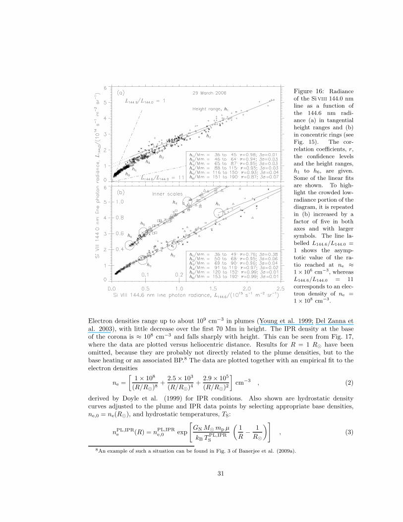
Figure 16: Radianceof the Siviii 144.0 nmline as a function ofthe 144.6 nm radi-ance (a) in tangentialheight ranges and (b)in concentric rings (seeFig. 15). The cor-relation coefficients, r,the confidence levelsand the height ranges,h1 to h6, are given.Some of the linear fitsare shown. To high-light the crowded low-radiance portion of thediagram, it is repeatedin (b) increased by afactor of five in bothaxes and with largersymbols. The line la-belled L144.6/L144.0 =1 shows the asymp-totic value of the ra-tio reached at ne ≈

1× 106 cm−3, whereasL144.6/L144.0 = 11corresponds to an elec-tron density of ne =1× 108 cm−3.

Electron densities range up to about 109 cm−3 in plumes (Young et al. 1999; Del Zanna etal. 2003), with little decrease over the first 70 Mm in height. The IPR density at the baseof the corona is ≈ 108 cm−3 and falls sharply with height. This can be seen from Fig. 17,where the data are plotted versus heliocentric distance. Results for R = 1 R⊙ have beenomitted, because they are probably not directly related to the plume densities, but to thebase heating or an associated BP.8 The data are plotted together with an empirical fit to theelectron densities

ne =

[

1× 108

(R/R⊙)8+

2.5× 103

(R/R⊙)4+

2.9× 105

(R/R⊙)2

]

cm−3 , (2)

derived by Doyle et al. (1999) for IPR conditions. Also shown are hydrostatic densitycurves adjusted to the plume and IPR data points by selecting appropriate base densities,ne,0 = ne(R⊙), and hydrostatic temperatures, TS:

nPL,IPRe (R) = nPL,IPR

e,0 exp

[

GN M⊙ mp µ

kB TPL,IPRS

(

1

R− 1

R⊙

)

]

, (3)

8An example of such a situation can be found in Fig. 3 of Banerjee et al. (2009a).

31

where GN is the gravitational constant, M⊙ the mass of the Sun, mp the proton mass, kBthe Boltzmann constant and µ = 0.56 for a fractional helium abundance of nα/np = 5 % (cf.,Bame et al. 1977). However, with the high outflow speeds that have been observed in IPRs,the hydrostatic model does, in all likelihood, not provide a viable option for that case.

Considering that the various data points and the fits have been obtained with the help ofdifferent methods and observations of many plumes and IPRs spread over several years intwo sunspot minimum periods, it must be concluded that the excellent agreement can onlybe explained, if CH conditions in general are remarkably stable. It therefore appears tobe reasonable to assume standard plume and IPR densities close to the graphs in Fig. 17and examine, in particular, the density ratio between these plasma regimes. If we take thepower-law fits at face value, we find a plume-IPR density ratio of three below R = 2 R⊙ withne ∝ (R⊙/R)8 both in plumes and IPRs. Above R = 3 R⊙, it is n

PLe ∝ (R⊙/R)3, whereas the

IPR density nIPRe is proportional to (R⊙/R)2. In the low corona, the densities of plumes and

IPRs thus decline at the same rate. Higher up, the plume densities seem to decrease fasterthan those of IPRs and the density ratio becomes smaller. This ratio is four to seven in thelow corona from WL eclipse observations, but, in general, the value is near two if obtainedfrom LOS line-ratio studies, such as that in Fig. 15. This discrepancy could be resolved bythe above consideration of density variations along the LOS caused by two plasma regimes inFig. 16, leading to density ratios in agreement with WL observations.

5.2 Plasma temperatures and non-thermal motions

5.2.1 Electron temperature

Early electron-temperature determinations of CH plasmas have been summarized by Habbalet al. (1993). Data obtained in wavelength ranges from X-rays to WL as well as charge-state measurements have been considered together with relevant evaluation methods. Theconclusion was that large uncertainties have to be accepted and that Te increases in CHsbetween h > 0 and h = 0.6 R⊙ from 0.8 MK to ≈ 1.3 MK with some indication of highertemperatures on the disk.

Typical temperatures found in CHs, IPRs and plumes (using methods described below) duringthe last two decades are summarized in Table 4 and Fig. 18. It appears as if the temperatureincrease with height in CHs is mainly related to IPRs, but is not typical for plumes. Theelectron temperature in the solar corona can be measured using several different methods,most of them depend, at this stage, on the observations of electromagnetic radiation fromatoms and ions: Under the assumption of ionization equilibrium, the ionic fractions of thevarious species in a plasma as a function of the electron temperature can be determined (cf.,e.g., Mazzotta et al. 1998). The excitation and de-activation processes of the species alsodepend on the electron temperature. For allowed transitions, spontaneous photon emission,in general, is the dominant de-activation process. It is controlled by the contribution function

Gjg(Te) =ng

nX

1√Te

exp

(−∆ǫgjkB Te

)

, (4)

where ng/nX is the ionic fraction of the element X, if most of the ions are in the ground stateand ∆ǫgj the energy difference between the states g and j (cf., Pottasch 1963; Gabriel andJordan 1973; Mariska 1992; Wilhelm et al. 2004).

32

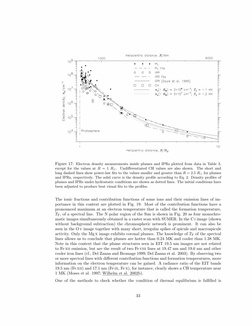
Figure 17: Electron density measurements inside plumes and IPRs plotted from data in Table 3,except for the values at R = 1 R⊙. Undifferentiated CH values are also shown. The short andlong dashed lines show power-law fits to the values smaller and greater than R = 2.5 R⊙ for plumesand IPRs, respectively. The solid curve is the density profile according to Eq. 2. Density profiles ofplumes and IPRs under hydrostatic conditions are shown as dotted lines. The initial conditions havebeen adjusted to produce best visual fits to the profiles.

The ionic fractions and contribution functions of some ions and their emission lines of im-portance in this context are plotted in Fig. 19. Most of the contribution functions have apronounced maximum at an electron temperature that is called the formation temperature,TF, of a spectral line. The N polar region of the Sun is shown in Fig. 20 as four monochro-matic images simultaneously obtained in a raster scan with SUMER. In the C i image (shownwithout background subtraction) the chromospheric network is prominent. It can also beseen in the Ov image together with many short, irregular spikes of spicule and macrospiculeactivity. Only the Mgx image exhibits coronal plumes. The knowledge of TF of the spectrallines allows us to conclude that plumes are hotter than 0.24 MK and cooler than 1.38 MK.Note in this context that the plume structures seen in EIT 19.5 nm images are not relatedto Fexii emission, but are the result of two Feviii lines at 19.47 nm and 19.6 nm and othercooler iron lines (cf., Del Zanna and Bromage 1999; Del Zanna et al. 2003). By observing twoor more spectral lines with different contribution functions and formation temperatures, moreinformation on the electron temperature can be gained. A radiance ratio of the EIT bands19.5 nm (Fexii) and 17.1 nm (Fe ix, Fex), for instance, clearly shows a CH temperature near1 MK (Moses et al. 1997; Wilhelm et al. 2002b).

One of the methods to check whether the condition of thermal equilibrium is fulfilled is

33

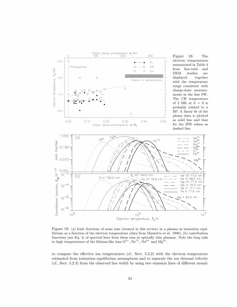
Figure 18: Theelectron temperaturessummarized in Table 4from line-ratio andDEM studies aredisplayed togetherwith the temperaturerange consistent withcharge-state measure-ments in the fast SW.The CH temperatureof 2 MK at h = 0 isprobably related to aBP. A linear fit of theplume data is plottedas solid line and thatfor the IPR values asdashed line.

Figure 19: (a) Ionic fractions of some ions (treated in this review) in a plasma in ionization equi-librium as a function of the electron temperature (data from Mazzotta et al. 1998); (b) contributionfunctions (see Eq. 4) of spectral lines from these ions in optically thin plasmas. Note the long tailsto high temperatures of the lithium-like ions O5+, Ne7+, Na8+ and Mg9+.

to compare the effective ion temperatures (cf., Sect. 5.2.2) with the electron temperatureestimated from ionization equilibrium assumptions and to separate the ion thermal velocity(cf., Sect. 5.2.3) from the observed line width by using two emission lines of different atomic

34

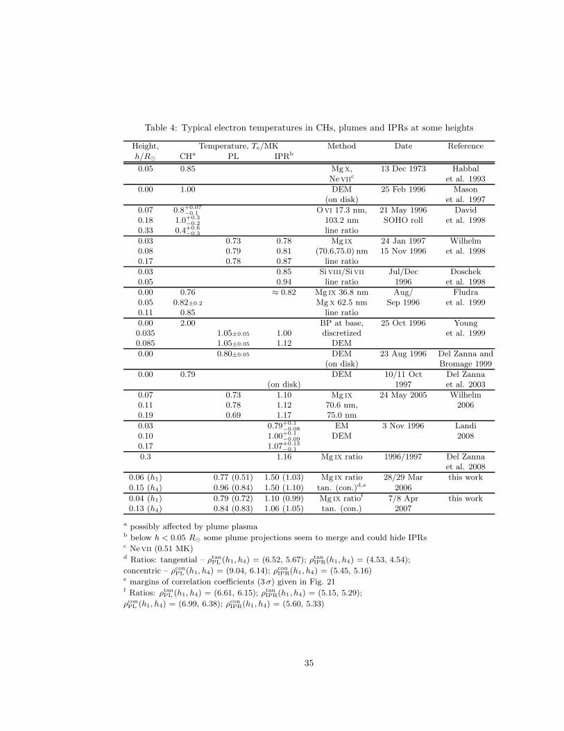
Table 4: Typical electron temperatures in CHs, plumes and IPRs at some heights

Height, Temperature, Te/MK Method Date Reference

h/R⊙ CHa PL IPRb

0.05 0.85 Mgx, 13 Dec 1973 HabbalNeviic et al. 1993

0.00 1.00 DEM 25 Feb 1996 Mason(on disk) et al. 1997

0.07 0.8+0.07−0.1 Ovi 17.3 nm, 21 May 1996 David

0.18 1.0+0.3−0.2 103.2 nm SOHO roll et al. 1998

0.33 0.4+0.6−0.3 line ratio

0.03 0.73 0.78 Mg ix 24 Jan 1997 Wilhelm0.08 0.79 0.81 (70.6,75.0) nm 15 Nov 1996 et al. 19980.17 0.78 0.87 line ratio

0.03 0.85 Siviii/Sivii Jul/Dec Doschek0.05 0.94 line ratio 1996 et al. 1998

0.00 0.76 ≈ 0.82 Mg ix 36.8 nm Aug/ Fludra0.05 0.82±0.2 Mgx 62.5 nm Sep 1996 et al. 19990.11 0.85 line ratio

0.00 2.00 BP at base, 25 Oct 1996 Young0.035 1.05±0.05 1.00 discretized et al. 19990.085 1.05±0.05 1.12 DEM

0.00 0.80±0.05 DEM 23 Aug 1996 Del Zanna and(on disk) Bromage 1999

0.00 0.79 DEM 10/11 Oct Del Zanna(on disk) 1997 et al. 2003

0.07 0.73 1.10 Mg ix 24 May 2005 Wilhelm0.11 0.78 1.12 70.6 nm, 20060.19 0.69 1.17 75.0 nm

0.03 0.79+0.1−0.08 EM 3 Nov 1996 Landi

0.10 1.00+0.1−0.09 DEM 2008

0.17 1.07+0.13−0.1

0.3 1.16 Mg ix ratio 1996/1997 Del Zannaet al. 2008

0.06 (h1) 0.77 (0.51) 1.50 (1.03) Mg ix ratio 28/29 Mar this work

0.15 (h4) 0.96 (0.84) 1.50 (1.10) tan. (con.)d,e 2006

0.04 (h1) 0.79 (0.72) 1.10 (0.99) Mg ix ratiof 7/8 Apr this work0.13 (h4) 0.84 (0.83) 1.06 (1.05) tan. (con.) 2007

a possibly affected by plume plasmab below h < 0.05 R⊙ some plume projections seem to merge and could hide IPRsc Nevii (0.51 MK)d Ratios: tangential – ρtanPL (h1, h4) = (6.52, 5.67); ρtanIPR(h1, h4) = (4.53, 4.54);

concentric – ρconPL (h1, h4) = (9.04, 6.14); ρconIPR(h1, h4) = (5.45, 5.16)e margins of correlation coefficients (3σ) given in Fig. 21f Ratios: ρtanPL (h1, h4) = (6.61, 6.15); ρtanIPR(h1, h4) = (5.15, 5.29);

ρconPL (h1, h4) = (6.99, 6.38); ρconIPR(h1, h4) = (5.60, 5.33)

35

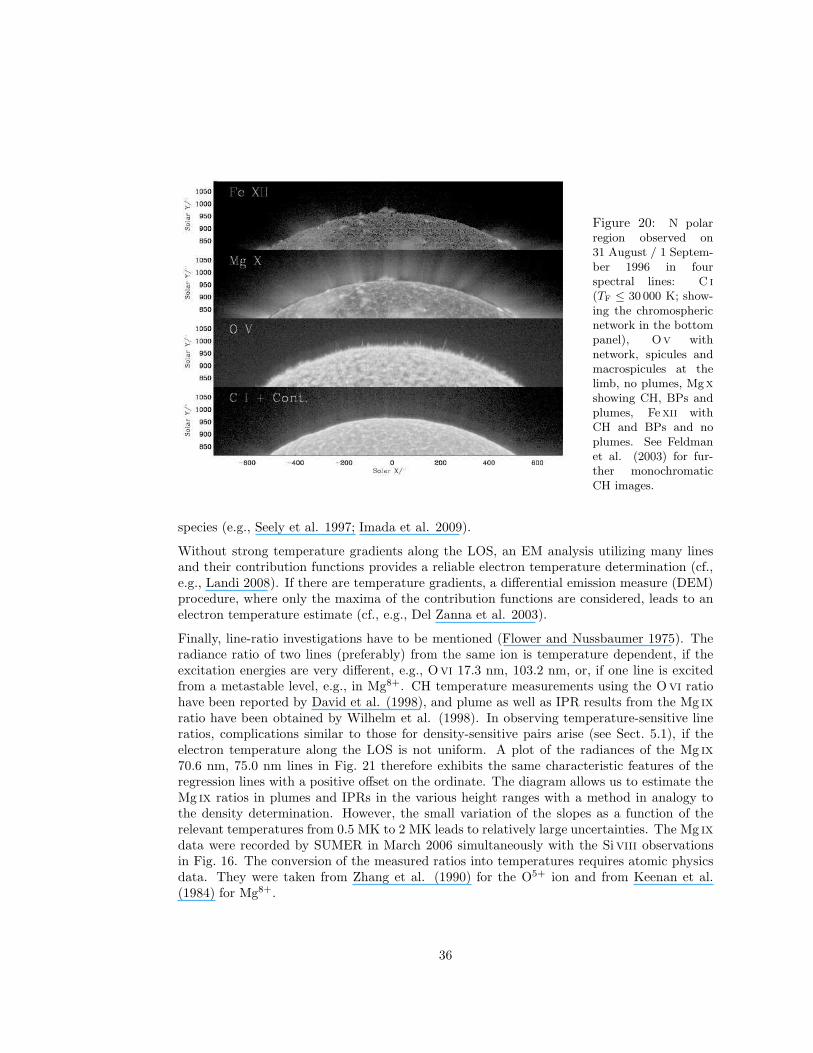
Figure 20: N polarregion observed on31 August / 1 Septem-ber 1996 in fourspectral lines: C i(TF ≤ 30 000 K; show-ing the chromosphericnetwork in the bottompanel), Ov withnetwork, spicules andmacrospicules at thelimb, no plumes, Mgxshowing CH, BPs andplumes, Fexii withCH and BPs and noplumes. See Feldmanet al. (2003) for fur-ther monochromaticCH images.

species (e.g., Seely et al. 1997; Imada et al. 2009).

Without strong temperature gradients along the LOS, an EM analysis utilizing many linesand their contribution functions provides a reliable electron temperature determination (cf.,e.g., Landi 2008). If there are temperature gradients, a differential emission measure (DEM)procedure, where only the maxima of the contribution functions are considered, leads to anelectron temperature estimate (cf., e.g., Del Zanna et al. 2003).

Finally, line-ratio investigations have to be mentioned (Flower and Nussbaumer 1975). Theradiance ratio of two lines (preferably) from the same ion is temperature dependent, if theexcitation energies are very different, e.g., Ovi 17.3 nm, 103.2 nm, or, if one line is excitedfrom a metastable level, e.g., in Mg8+. CH temperature measurements using the Ovi ratiohave been reported by David et al. (1998), and plume as well as IPR results from the Mg ixratio have been obtained by Wilhelm et al. (1998). In observing temperature-sensitive lineratios, complications similar to those for density-sensitive pairs arise (see Sect. 5.1), if theelectron temperature along the LOS is not uniform. A plot of the radiances of the Mg ix70.6 nm, 75.0 nm lines in Fig. 21 therefore exhibits the same characteristic features of theregression lines with a positive offset on the ordinate. The diagram allows us to estimate theMg ix ratios in plumes and IPRs in the various height ranges with a method in analogy tothe density determination. However, the small variation of the slopes as a function of therelevant temperatures from 0.5 MK to 2 MK leads to relatively large uncertainties. The Mg ixdata were recorded by SUMER in March 2006 simultaneously with the Siviii observationsin Fig. 16. The conversion of the measured ratios into temperatures requires atomic physicsdata. They were taken from Zhang et al. (1990) for the O5+ ion and from Keenan et al.(1984) for Mg8+.

36

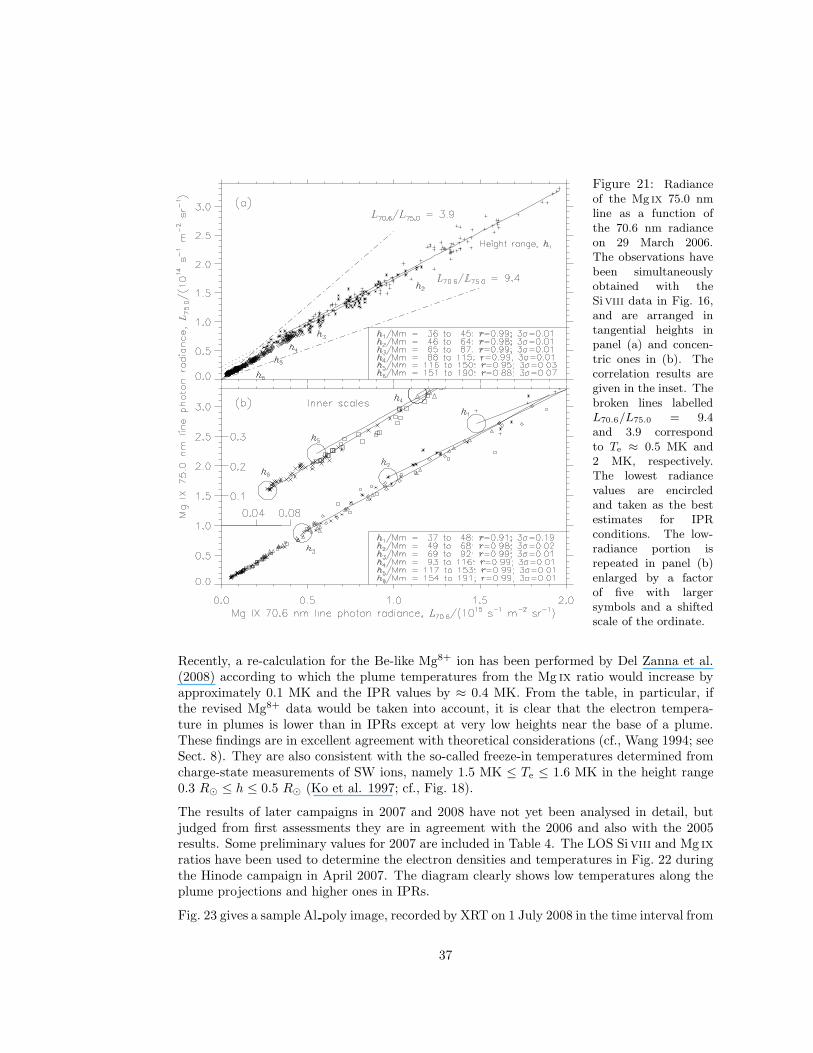
Figure 21: Radianceof the Mg ix 75.0 nmline as a function ofthe 70.6 nm radianceon 29 March 2006.The observations havebeen simultaneouslyobtained with theSiviii data in Fig. 16,and are arranged intangential heights inpanel (a) and concen-tric ones in (b). Thecorrelation results aregiven in the inset. Thebroken lines labelledL70.6/L75.0 = 9.4and 3.9 correspondto Te ≈ 0.5 MK and2 MK, respectively.The lowest radiancevalues are encircledand taken as the bestestimates for IPRconditions. The low-radiance portion isrepeated in panel (b)enlarged by a factorof five with largersymbols and a shiftedscale of the ordinate.

Recently, a re-calculation for the Be-like Mg8+ ion has been performed by Del Zanna et al.(2008) according to which the plume temperatures from the Mg ix ratio would increase byapproximately 0.1 MK and the IPR values by ≈ 0.4 MK. From the table, in particular, ifthe revised Mg8+ data would be taken into account, it is clear that the electron tempera-ture in plumes is lower than in IPRs except at very low heights near the base of a plume.These findings are in excellent agreement with theoretical considerations (cf., Wang 1994; seeSect. 8). They are also consistent with the so-called freeze-in temperatures determined fromcharge-state measurements of SW ions, namely 1.5 MK ≤ Te ≤ 1.6 MK in the height range0.3 R⊙ ≤ h ≤ 0.5 R⊙ (Ko et al. 1997; cf., Fig. 18).

The results of later campaigns in 2007 and 2008 have not yet been analysed in detail, butjudged from first assessments they are in agreement with the 2006 and also with the 2005results. Some preliminary values for 2007 are included in Table 4. The LOS Siviii and Mg ixratios have been used to determine the electron densities and temperatures in Fig. 22 duringthe Hinode campaign in April 2007. The diagram clearly shows low temperatures along theplume projections and higher ones in IPRs.

Fig. 23 gives a sample Al poly image, recorded by XRT on 1 July 2008 in the time interval from

37

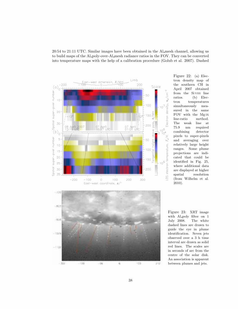
20:54 to 21:11 UTC. Similar images have been obtained in the Al mesh channel, allowing usto build maps of the Al poly-over-Al mesh radiance ratios in the FOV. They can be convertedinto temperature maps with the help of a calibration procedure (Golub et al. 2007). Dashed

Figure 22: (a) Elec-tron density map ofthe southern CH inApril 2007 obtainedfrom the Siviii lineratios. (b) Elec-tron temperaturessimultaneously mea-sured in the sameFOV with the Mg ixline-ratio method.The weak line at75.9 nm requiredcombining detectorpixels to super-pixelsand averaging overrelatively large heightranges. Some plumeprojections are indi-cated that could beidentified in Fig. 25,where additional dataare displayed at higherspatial resolution(from Wilhelm et al.2010).

Figure 23: XRT imagewith Al poly filter on 1July 2008. The whitedashed lines are drawn toguide the eye in plumeidentification. Seven jetsobserved over a 3 h timeinterval are drawn as solidred lines. The scales arein seconds of arc from thecentre of the solar disk.An association is apparentbetween plumes and jets.

38

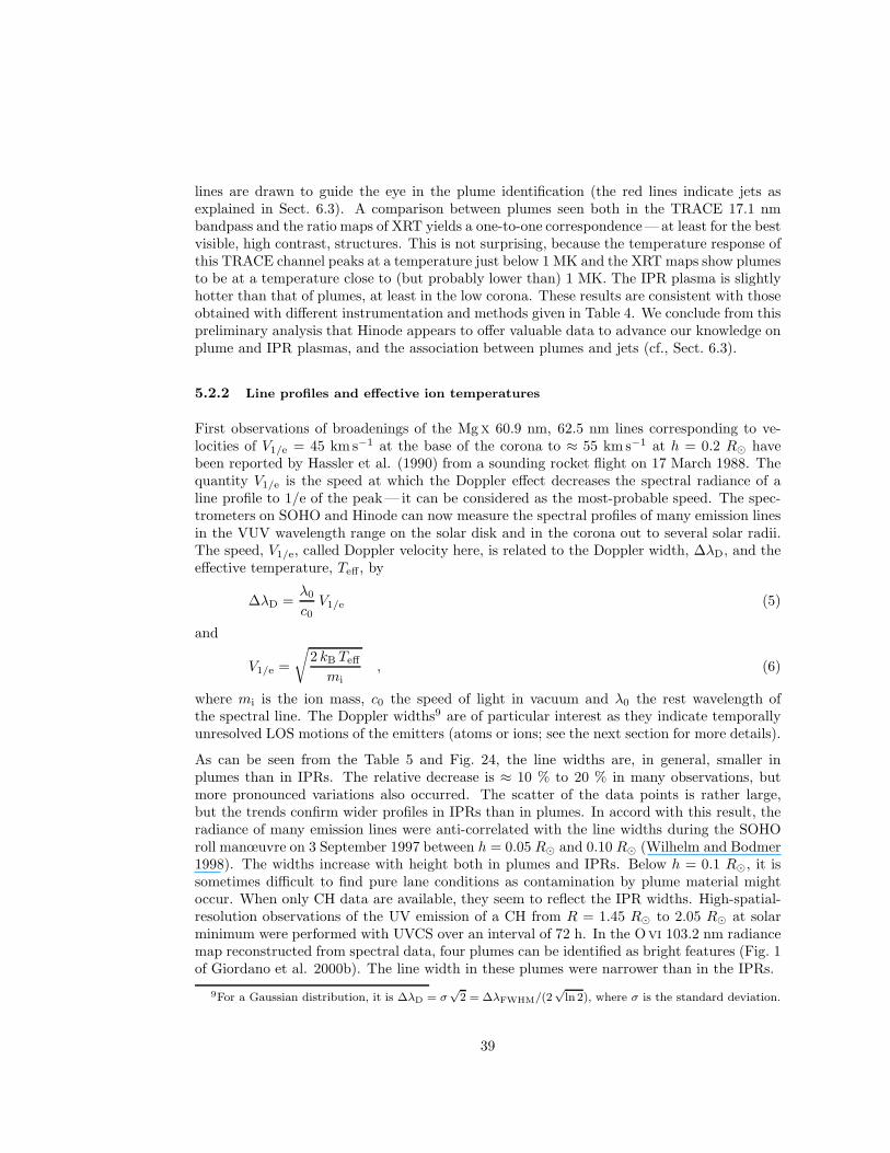
lines are drawn to guide the eye in the plume identification (the red lines indicate jets asexplained in Sect. 6.3). A comparison between plumes seen both in the TRACE 17.1 nmbandpass and the ratio maps of XRT yields a one-to-one correspondence—at least for the bestvisible, high contrast, structures. This is not surprising, because the temperature response ofthis TRACE channel peaks at a temperature just below 1 MK and the XRT maps show plumesto be at a temperature close to (but probably lower than) 1 MK. The IPR plasma is slightlyhotter than that of plumes, at least in the low corona. These results are consistent with thoseobtained with different instrumentation and methods given in Table 4. We conclude from thispreliminary analysis that Hinode appears to offer valuable data to advance our knowledge onplume and IPR plasmas, and the association between plumes and jets (cf., Sect. 6.3).

5.2.2 Line profiles and effective ion temperatures

First observations of broadenings of the Mgx 60.9 nm, 62.5 nm lines corresponding to ve-locities of V1/e = 45 km s−1 at the base of the corona to ≈ 55 km s−1 at h = 0.2 R⊙ havebeen reported by Hassler et al. (1990) from a sounding rocket flight on 17 March 1988. Thequantity V1/e is the speed at which the Doppler effect decreases the spectral radiance of aline profile to 1/e of the peak— it can be considered as the most-probable speed. The spec-trometers on SOHO and Hinode can now measure the spectral profiles of many emission linesin the VUV wavelength range on the solar disk and in the corona out to several solar radii.The speed, V1/e, called Doppler velocity here, is related to the Doppler width, ∆λD, and theeffective temperature, Teff , by

∆λD =λ0

c0V1/e (5)

and

V1/e =

√

2 kB Teff

mi

, (6)

where mi is the ion mass, c0 the speed of light in vacuum and λ0 the rest wavelength ofthe spectral line. The Doppler widths9 are of particular interest as they indicate temporallyunresolved LOS motions of the emitters (atoms or ions; see the next section for more details).

As can be seen from the Table 5 and Fig. 24, the line widths are, in general, smaller inplumes than in IPRs. The relative decrease is ≈ 10 % to 20 % in many observations, butmore pronounced variations also occurred. The scatter of the data points is rather large,but the trends confirm wider profiles in IPRs than in plumes. In accord with this result, theradiance of many emission lines were anti-correlated with the line widths during the SOHOroll manœuvre on 3 September 1997 between h = 0.05 R⊙ and 0.10 R⊙ (Wilhelm and Bodmer1998). The widths increase with height both in plumes and IPRs. Below h = 0.1 R⊙, it issometimes difficult to find pure lane conditions as contamination by plume material mightoccur. When only CH data are available, they seem to reflect the IPR widths. High-spatial-resolution observations of the UV emission of a CH from R = 1.45 R⊙ to 2.05 R⊙ at solarminimum were performed with UVCS over an interval of 72 h. In the Ovi 103.2 nm radiancemap reconstructed from spectral data, four plumes can be identified as bright features (Fig. 1of Giordano et al. 2000b). The line width in these plumes were narrower than in the IPRs.

9For a Gaussian distribution, it is ∆λD = σ√2 = ∆λFWHM/(2

√ln 2), where σ is the standard deviation.

39

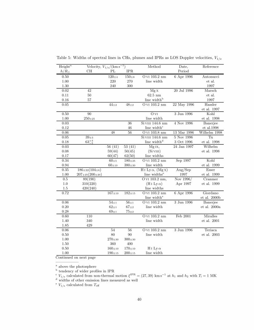
Table 5: Widths of spectral lines in CHs, plumes and IPRs as LOS Doppler velocities, V1/e

Heighta Velocity, V1/e/(km s−1) Method Date, Referenceh/R⊙ CH PL IPR Period

0.50 120±4 150±8 Ovi 103.2 nm 6 Apr 1996 Antonucci1.00 220 270 line width et al.1.30 240 300 1997

0.02 42 Mgx 20 Jul 1996 Marsch0.11 50 62.5 nm et al.

0.16 57 line widthb 1997

0.05 44±2 48±2 Ovi 103.2 nm 22 May 1996 Hassleret al. 1997

0.50 90 Ovi 3 Jun 1996 Kohl1.00 250±25 line width et al. 1998

0.03 36 Siviii 144.6 nm 4 Nov 1996 Banerjee0.12 46 line widthc et al.1998

0.06 48 56 Ovi 103.8 nm 13 Mar 1996 Wilhelm 1998

0.05 39±3 Siviii 144.6 nm 5 Nov 1996 Tu0.18 63+4

−5 line widthd 3 Oct 1996 et al. 1998

0.03 56 (41) 53 (41) Mg ix, 24 Jan 1997 Wilhelm0.08 59(44) 50(45) (Siviii) et al. 19980.17 60(47) 62(50) line widths

0.34 60±5 180±25 Ovi 103.2 nm Sep 1997 Kohl0.94 60±10 380±30 line width et al. 1999

0.35 186±22(104±6) H i Lyα, (Mgx) Aug/Sep Esser1.00 207±25(200±20) line widthse 1997 et al. 1999

0.5 89(190) Ovi 103.2 nm, Nov 1996/ Cranmer1.0 310(220) (H i Lyα) Apr 1997 et al. 19991.5 420(240) line widths

0.72 167±10 182±15 Ovi 103.2 nm 6 Apr 1996 Giordanoline widthe et al. 2000b

0.06 54±1 56±1 Ovi 103.2 nm 3 Jun 1996 Banerjee0.20 62±1 67±2 line width et al. 2000a0.28 69±1 75±2

0.60 110 Ovi 103.2 nm Feb 2001 Miralles1.40 340 line width et al. 20011.85 429

0.06 54 56 Ovi 103.2 nm 3 Jun 1996 Teriaca0.50 80 90 line width et al. 20031.00 270±30 300±30

1.50 360 4000.50 160±10 170±10 H i Lyα1.00 190±15 200±15 line width

Continued on next page——————a above the photosphereb tendency of wider profiles in IPRc V1/e calculated from non-thermal motion ξIPR = (27, 39) kms−1 at h1 and h2 with Ti = 1 MKd widths of other emission lines measured as welle V1/e calculated from Teff

40

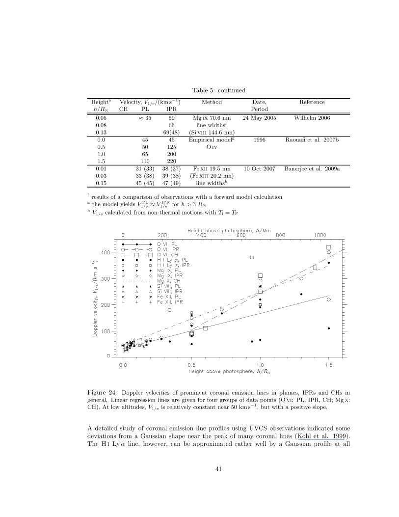
Table 5: continued

Heighta Velocity, V1/e/(km s−1) Method Date, Referenceh/R⊙ CH PL IPR Period

0.05 ≈ 35 59 Mg ix 70.6 nm 24 May 2005 Wilhelm 20060.08 66 line widthsf

0.13 69(48) (Siviii 144.6 nm)

0.0 45 45 Empirical modelg 1996 Raouafi et al. 2007b0.5 50 125 O iv1.0 65 2001.5 110 220

0.01 31 (33) 38 (37) Fexii 19.5 nm 10 Oct 2007 Banerjee et al. 2009a0.03 33 (38) 39 (38) (Fexiii 20.2 nm)

0.15 45 (45) 47 (49) line widthsh

f results of a comparison of observations with a forward model calculationg the model yields V PL

1/e ≈ V IPR1/e for h > 3 R⊙

h V1/e calculated from non-thermal motions with Ti = TF

Figure 24: Doppler velocities of prominent coronal emission lines in plumes, IPRs and CHs ingeneral. Linear regression lines are given for four groups of data points (Ovi: PL, IPR, CH; Mgx:CH). At low altitudes, V1/e is relatively constant near 50 kms−1, but with a positive slope.

A detailed study of coronal emission line profiles using UVCS observations indicated somedeviations from a Gaussian shape near the peak of many coronal lines (Kohl et al. 1999).The H i Lyα line, however, can be approximated rather well by a Gaussian profile at all

41

heights, whereas the Ovi profiles are more complex: at low altitudes (below h ≈ 0.35 R⊙)they are nearly Gaussians, but more pronounced deviations occur at greater heights. TheOvi profiles can be represented there by narrow and broad components. The latter appearsto be associated with low-density IPRs, and the former with denser plumes along the LOS.They are mainly observed at the centre of the line close to the rest wavelength, so that nosignificant Doppler shifts are observed for these plume contributions. The width of the narrowcomponent hardly changes with height. Beyond R = 2.5 R⊙, the line profiles are formed onlyby the broad component, and the narrow component is no longer observed.

For SUMER observations from low altitudes, the separation of a narrow plume line profilefrom a somewhat wider IPR contribution is not easy. In a forward calculation, the observedline widths in Mg ix 70.6 nm could be reproduced under the assumption of a constant V1/e =35 km s−1 over a height range from 0.05 R⊙ to 0.13 R⊙ and the IPR widths nearly twiceas wide (see Table 5). This result would explain the observations by Doschek et al. (2001)indicating line-width increases with height for Siviii 144.6 nm on 3 May 1996 and no effectfor several ions on 3 November 1996, if the SUMER slit was aligned with an IPR in Mayand with a plume in November. It should be mentioned here that Banerjee et al. (2000a)and Xia et al. (2004) found wider Ovi line widths in plumes (or near their footpoints) thanin darker regions on the disk. We also have to note that the V1/e speeds of O5+ ions aremuch higher than those of Si7+ in IPR (Banerjee et al. 2000a), and that magnesium ionshave higher speeds than hydrogen (Esser et al. 1999) or Si7+ (Wilhelm et al. 1998; Wilhelm2006). Finally, O5+ exhibits about twice the difference in V1/e between plumes and IPR thanhydrogen at h ≈ 0.5 R⊙ to 1 R⊙ (Giordano et al. 1997).

5.2.3 Ion temperatures and non-thermal motions

The Doppler width, ∆λD, of an emission line is caused by the thermal motions along theLOS of the atom or ion under study and the non-thermal contributions, which are eitherturbulence or temporally unresolved waves. We can thus write

∆λD =λ0

c0

√

2 kB Ti

mi

+ ξ2 , (7)

where Ti is the ion temperature and ξ the non-thermal speed (cf., Mariska 1992).

Under the assumption of Ti = 1 MK for Si7+ ions, Banerjee et al. (1998) derived non-thermalmotions of 27 km s−1 at 0.03 R⊙ above the limb in PCHs and 46 km s−1 at 0.26 R⊙. Bothvalues were obtained in IPR. An ion temperature of 2 MK did not lead to a consistent result.Hassler et al. (1997) and Banerjee et al. (2000a) put forward the hypothesis that the iontemperatures in plumes and IPRs are not very different, but that higher non-thermal motionsare present in IPRs.

The non-thermal speed is related to the wave amplitude by ξ2 = 〈δv2〉/ζ (with ζ ≈ 2 de-pending on the polarization and LOS), if waves are responsible for this contribution (cf., e.g.,Hassler et al. 1990). Variations of ξ as function of height above the limb have been calcu-lated from EIS observations in the lines Fexii 19.5 nm and Fexiii 20.2 nm (Banerjee et al.2009a). Since the separation of V1/e into Ti and ξ is not a straightforward procedure—asdiscussed in detail by Dolla and Solomon (2008)—we include in Table 5 only LOS Doppler

42

velocities directly derived from line-width measurements or calculated from ξ and Ti data inthe literature.

5.3 Elemental abundances and first ionization potentials

The composition of the solar photosphere can, with the exception of the noble gases, bedirectly determined from spectroscopic observations (cf., Grevesse and Sauval 1998). In thecorona, attempts to measure the helium abundance have been made by Gabriel et al. (1986)and Laming and Feldman (2001); for argon and neon abundances see Phillips et al. (2003) andLandi et al. (2007). Methods of measuring the solar and coronal abundances of an element Xhave been reviewed by von Steiger et al. (2001). In the corona, the abundance of elementsis varying and the so-called FIP effect seems to play a dominant role. Elements with a FIPof IX < 10 eV are defined as low-FIP elements and those with FIP of IX > 10 eV as high-FIP elements, separated by the photon energy h ν = 10 eV of the H i Lyα line. The low-FIPelements are—with respect to photospheric values—overabundant in the (equatorial) coronaby a factor of about four to five relative to the high-FIP elements (cf., Widing et al. 2005).The magnesium/neon abundance ratio in plumes is enhanced relative to IPRs by a factorof 1.5 (Young et al. 1999) to 1.7 at h = 0.05 R⊙ and 3.5 at 0.1 R⊙ (Wilhelm and Bodmer1998). These abundance determinations depend on the electron temperatures employed, andmight have to be re-evaluated should better temperature data become available. According toFeldman et al. (1998), there was no significant FIP effect observed at h = 0.03 R⊙ above thenorthern solar limb on 3 November 1996; these data were taken by SUMER in an IPR of a CH(cf., Landi 2008). If the IPRs are indeed the source regions of the fast SW, no compositionchanges would be expected in the high-speed streams in accordance with observations, exceptprobably for helium with its long first ionization time (FIT) (Geiss et al. 1995).

Observations of the Neviii 77.0 nm and Mgviii 77.2 nm lines in April 2007 during the mostrecent solar minimum showed a very clear plume/IPR structure in a map of the radianceratio L77.0/L77.2 (Curdt et al. 2008), which is repeated in Fig. 25(a). Any doubt that thiseffect is caused by the high-temperature tail of the lithium-like Neviii contribution function(see Fig. 19) can be dispelled by inspecting Fig. 25(b) and (d) showing radiance ratios of theNeviii line with the Mg ix and Na ix 69.4 nm (0.85 MK) lines.10 Although these lines havedifferent contribution functions compared to Mgviii, the plume/IPR patterns are basicallythe same. In particular, as the contribution function of Na ix is always larger than that ofNeviii above 0.8 MK, it must be concluded that a FIP effect in plumes operates with anenhancement of the magnesium abundance by a factor of 1.5 to 2 relative to neon, and thatthe relative abundance of the low-FIP element sodium is enhanced as well. A verificationthat there are higher electron temperatures in IPRs than in plumes follows from Fig. 25(e)displaying the L(Siviii)/L(Si ix) radiance ratio.

Widing and Feldman (2001) found in active regions (AR) that the confinement time of aplasma is a decisive parameter for abundance variations. A FIP bias of nearly ten wasreached after ≈ 6 d. If these findings can be applied to plumes, we would expect confinementtimes of a day or so—not too different from plume and BP lifetimes.

10Temperature effects, however, cause the high Neviii/Mg ix and Neviii/Na ix ratios at low altitudes inpanels (b) and (d), and the increase of the Neviii/Mgviii ratio in panel (a) above 120 Mm in the hot IPRs.

43

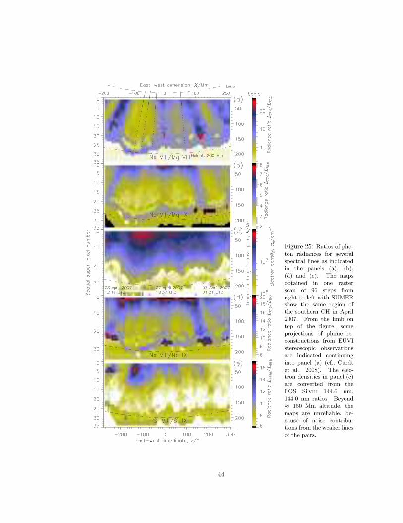
Figure 25: Ratios of pho-ton radiances for severalspectral lines as indicatedin the panels (a), (b),(d) and (e). The mapsobtained in one rasterscan of 96 steps fromright to left with SUMERshow the same region ofthe southern CH in April2007. From the limb ontop of the figure, someprojections of plume re-constructions from EUVIstereoscopic observationsare indicated continuinginto panel (a) (cf., Curdtet al. 2008). The elec-tron densities in panel (c)are converted from theLOS Siviii 144.6 nm,144.0 nm ratios. Beyond≈ 150 Mm altitude, themaps are unreliable, be-cause of noise contribu-tions from the weaker linesof the pairs.

44

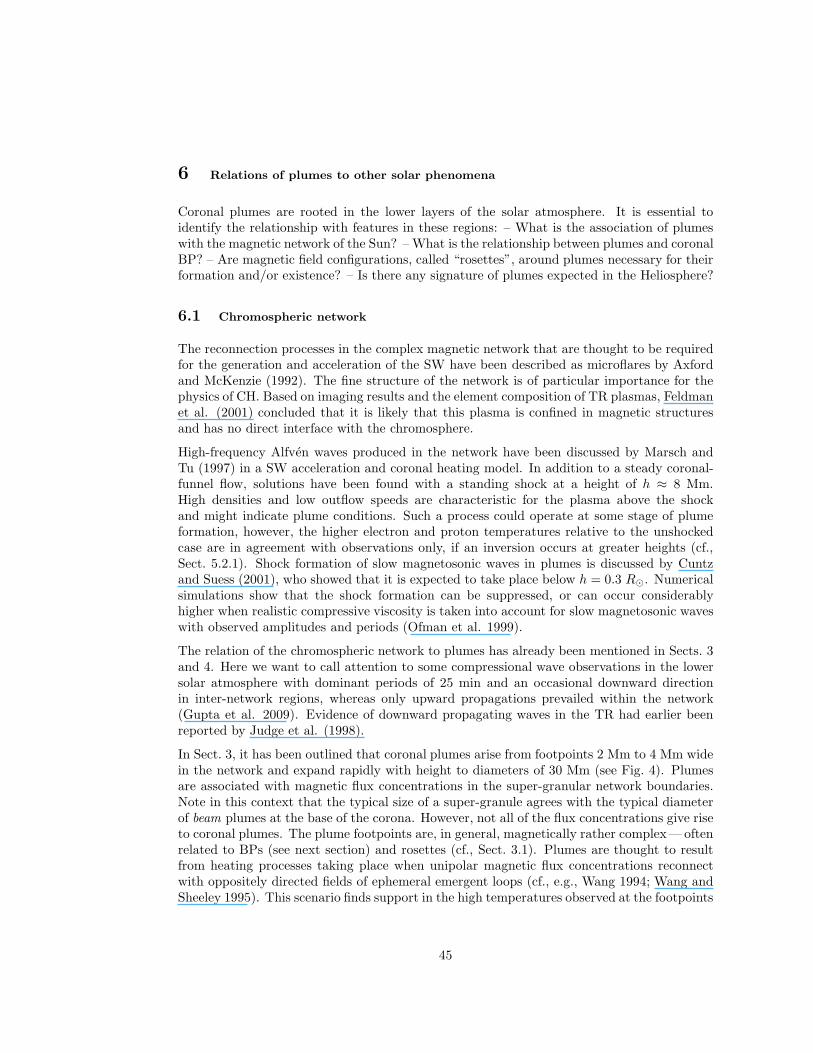
6 Relations of plumes to other solar phenomena

Coronal plumes are rooted in the lower layers of the solar atmosphere. It is essential toidentify the relationship with features in these regions: – What is the association of plumeswith the magnetic network of the Sun? – What is the relationship between plumes and coronalBP? – Are magnetic field configurations, called “rosettes”, around plumes necessary for theirformation and/or existence? – Is there any signature of plumes expected in the Heliosphere?

6.1 Chromospheric network

The reconnection processes in the complex magnetic network that are thought to be requiredfor the generation and acceleration of the SW have been described as microflares by Axfordand McKenzie (1992). The fine structure of the network is of particular importance for thephysics of CH. Based on imaging results and the element composition of TR plasmas, Feldmanet al. (2001) concluded that it is likely that this plasma is confined in magnetic structuresand has no direct interface with the chromosphere.

High-frequency Alfven waves produced in the network have been discussed by Marsch andTu (1997) in a SW acceleration and coronal heating model. In addition to a steady coronal-funnel flow, solutions have been found with a standing shock at a height of h ≈ 8 Mm.High densities and low outflow speeds are characteristic for the plasma above the shockand might indicate plume conditions. Such a process could operate at some stage of plumeformation, however, the higher electron and proton temperatures relative to the unshockedcase are in agreement with observations only, if an inversion occurs at greater heights (cf.,Sect. 5.2.1). Shock formation of slow magnetosonic waves in plumes is discussed by Cuntzand Suess (2001), who showed that it is expected to take place below h = 0.3 R⊙. Numericalsimulations show that the shock formation can be suppressed, or can occur considerablyhigher when realistic compressive viscosity is taken into account for slow magnetosonic waveswith observed amplitudes and periods (Ofman et al. 1999).

The relation of the chromospheric network to plumes has already been mentioned in Sects. 3and 4. Here we want to call attention to some compressional wave observations in the lowersolar atmosphere with dominant periods of 25 min and an occasional downward directionin inter-network regions, whereas only upward propagations prevailed within the network(Gupta et al. 2009). Evidence of downward propagating waves in the TR had earlier beenreported by Judge et al. (1998).

In Sect. 3, it has been outlined that coronal plumes arise from footpoints 2 Mm to 4 Mm widein the network and expand rapidly with height to diameters of 30 Mm (see Fig. 4). Plumesare associated with magnetic flux concentrations in the super-granular network boundaries.Note in this context that the typical size of a super-granule agrees with the typical diameterof beam plumes at the base of the corona. However, not all of the flux concentrations give riseto coronal plumes. The plume footpoints are, in general, magnetically rather complex—oftenrelated to BPs (see next section) and rosettes (cf., Sect. 3.1). Plumes are thought to resultfrom heating processes taking place when unipolar magnetic flux concentrations reconnectwith oppositely directed fields of ephemeral emergent loops (cf., e.g., Wang 1994; Wang andSheeley 1995). This scenario finds support in the high temperatures observed at the footpoints

45

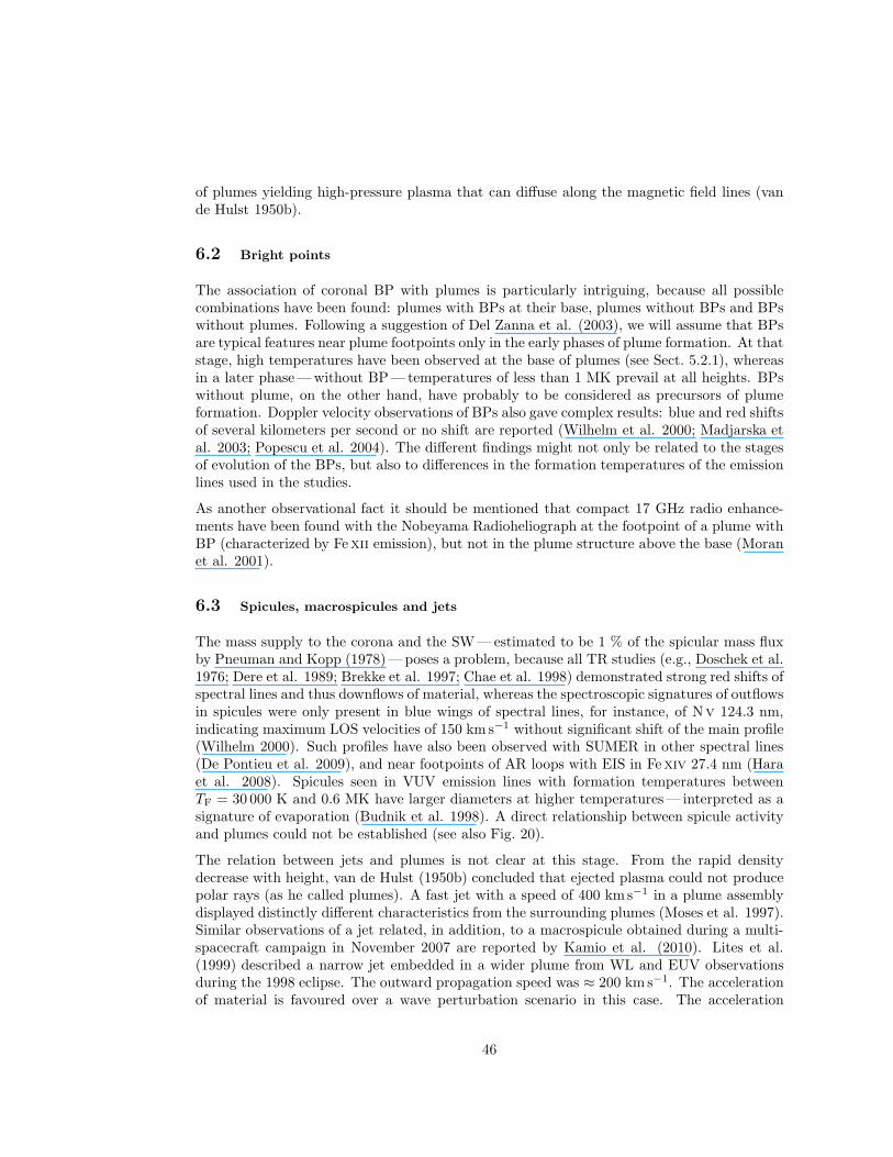
of plumes yielding high-pressure plasma that can diffuse along the magnetic field lines (vande Hulst 1950b).

6.2 Bright points

The association of coronal BP with plumes is particularly intriguing, because all possiblecombinations have been found: plumes with BPs at their base, plumes without BPs and BPswithout plumes. Following a suggestion of Del Zanna et al. (2003), we will assume that BPsare typical features near plume footpoints only in the early phases of plume formation. At thatstage, high temperatures have been observed at the base of plumes (see Sect. 5.2.1), whereasin a later phase—without BP—temperatures of less than 1 MK prevail at all heights. BPswithout plume, on the other hand, have probably to be considered as precursors of plumeformation. Doppler velocity observations of BPs also gave complex results: blue and red shiftsof several kilometers per second or no shift are reported (Wilhelm et al. 2000; Madjarska etal. 2003; Popescu et al. 2004). The different findings might not only be related to the stagesof evolution of the BPs, but also to differences in the formation temperatures of the emissionlines used in the studies.

As another observational fact it should be mentioned that compact 17 GHz radio enhance-ments have been found with the Nobeyama Radioheliograph at the footpoint of a plume withBP (characterized by Fexii emission), but not in the plume structure above the base (Moranet al. 2001).

6.3 Spicules, macrospicules and jets

The mass supply to the corona and the SW—estimated to be 1 % of the spicular mass fluxby Pneuman and Kopp (1978)—poses a problem, because all TR studies (e.g., Doschek et al.1976; Dere et al. 1989; Brekke et al. 1997; Chae et al. 1998) demonstrated strong red shifts ofspectral lines and thus downflows of material, whereas the spectroscopic signatures of outflowsin spicules were only present in blue wings of spectral lines, for instance, of Nv 124.3 nm,indicating maximum LOS velocities of 150 km s−1 without significant shift of the main profile(Wilhelm 2000). Such profiles have also been observed with SUMER in other spectral lines(De Pontieu et al. 2009), and near footpoints of AR loops with EIS in Fexiv 27.4 nm (Haraet al. 2008). Spicules seen in VUV emission lines with formation temperatures betweenTF = 30 000 K and 0.6 MK have larger diameters at higher temperatures— interpreted as asignature of evaporation (Budnik et al. 1998). A direct relationship between spicule activityand plumes could not be established (see also Fig. 20).

The relation between jets and plumes is not clear at this stage. From the rapid densitydecrease with height, van de Hulst (1950b) concluded that ejected plasma could not producepolar rays (as he called plumes). A fast jet with a speed of 400 kms−1 in a plume assemblydisplayed distinctly different characteristics from the surrounding plumes (Moses et al. 1997).Similar observations of a jet related, in addition, to a macrospicule obtained during a multi-spacecraft campaign in November 2007 are reported by Kamio et al. (2010). Lites et al.(1999) described a narrow jet embedded in a wider plume from WL and EUV observationsduring the 1998 eclipse. The outward propagation speed was ≈ 200 km s−1. The accelerationof material is favoured over a wave perturbation scenario in this case. The acceleration

46

Figure 26: A jet seenin the southern CH on 29March 2006 during the to-tal eclipse campaign em-bedded in plume and IPRstructures. The jet wasrecorded in Ovi line at103.2 nm and 103.8 nm(not shown) between 10:26and 11:23 UTC. The ratioL(103.2 nm)/L(103.8 nm)was 2.3 in the centre of thejet at 70 Mm height, justleft of it in plume plasmathe value was 2.35 and 2.4to the right in an IPR. Thesame event is shown in Fig 2as green rectangle. A super-pixel is equivalent to two de-tector pixels for this strongline.

could possibly be caused by explosive reconnection events (cf., Dere et al. 1991; Innes et al.1997). Explosive events observed in chromospheric and TR lines did not show any detectablesignature in the coronal Mgx 62.5 nm line (Teriaca et al. 2002; Doyle et al. 2004). However,the latter authors report their detection in the TRACE 17.1 nm channel. Thus a directgeneration of the coronal plasma by the explosive event can be excluded; however, an indirectprocess must operate in order to heat the plasma.

Correlated observations of EUV and WL jets with EIT and LASCO near the limb and atseveral solar radii showed that the bulk of the material travelled with a speed of ≈ 250 km s−1

much lower than the injection speeds (Wang et al. 1998). The jets originated near BPs and,in many cases, in the vicinity of plumes. Detailed studies of six polar jets observed in H i Lyαand Ovi by UVCS (some of them also seen by LASCO and EIT) indicated a relative decreasein line width during the jet brightenings comparable to the plume/IPR ratio (Dobrzycka etal. 2002). A pronounced plume-like brightening was observed in the northern CH duringthe total eclipse on 29 March 2006 from five different sites (Pasachoff et al. 2008). It wastherefore possible to determine an outward propagation speed of ≈ 65 km s−1 in the heightrange from h = 0.07 R⊙ to 0.27 R⊙. Based on the available data, the authors could notdecide whether the brightening was of a wave-like nature or a material jet. More or lesssimultaneously, a jet was observed in the southern CH by SUMER in the Ovi 103.2 nm,103.8 nm lines. It is shown in Fig. 26 together with plumes in the neighbourhood of the jet,which has a significantly different structure.

From XRT and EUVI observations in April 2007, Raouafi et al. (2008) found evidence thatjets are precursors of coronal plume formation. An example of a jet observed by EUVI aboardSTEREO A is recorded in Fig. 27 over a time period of 20 min showing in four images the

47

Figure 27: Observa-tions made by EUVIon STEREO A in the17.1 nm passband on7 April 2007 illustrat-ing a jet seen in thenegative prints. Itsevolution into a coro-nal plume occurredwithin 15 min. Thex and y coordinatescales are in secondsof arc from the centreof the solar disk (fromRaouafi et al. 2008).

transformation of a bright jet into plume haze interpreted as material on newly opened fieldlines. The base-heating model for plumes (Wang 1994) was applied to short-lived burst togenerate the jets in this model. The association of plumes and jets is confirmed by thepreliminary results of the Hinode campaign in summer 2008, where we found seven jets overa time interval of ≈ 3 h. They lasted from 4 min to 17 min, and most of them were seen inregions with prominent plumes. Fig. 23 shows the seven jets indicated as solid red lines inthe XRT Al poly image of a CH (see Sect. 5.2.1).

Twelve jets where detected during the 66 h LASCO-C2 observations in the right panel ofFig. 11. These features correspond to those jets-like structures seen by StCyr et al. (1997)above the polar regions and analysed by Wang et al. (1998). The conclusion was that theWL polar jets last for ≈ 2 h in the C2 FOV, their occurrence frequency is three to four perday with an angular width (measured with respect to their non-radial axis) of 2o to 4o; inagreement with the parameters deduced from the TID in Fig. 9. The super-radial expansionfactor of ≈ 2.2 reduces the angular width to 1o at the base of the corona (see DeForest et al.2001b). Recurrent WL polar jets reported by Wang et al. (1998) look like transient eventsdistinct from the quiescent emission of WL polar plumes. The main argument is the specificangular width and lifetime of these events. Some authors (e.g., Raouafi et al. 2008) foundevidence that jets are precursors of coronal plume formation. An TID analysis showed thatjets observed by LASCO-C2 in WL agree in duration, width and occurrence frequency withthose seen in the VUV by EIT and UVCS (Llebaria et al. 2002b). Nearly all of the jets inWL appear to be associated with bright plumes (at least in the projection plane of view).

48

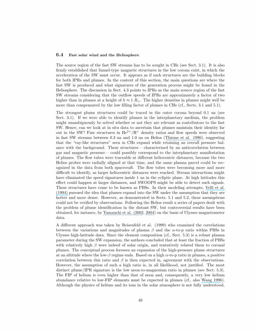
6.4 Fast solar wind and the Heliosphere

The source region of the fast SW streams has to be sought in CHs (see Sect. 3.1). It is alsofirmly established that funnel-type magnetic structures in the low corona exist, in which theacceleration of the SW must occur. It appears as if such structures are the building blocksfor both IPRs and plumes. In the context of this section, the main questions are where thefast SW is produced and what signatures of the generation process might be found in theHeliosphere. The discussion in Sect. 4.3 points to IPRs as the main source region of the fastSW streams considering that the outflow speeds of IPRs are approximately a factor of twohigher than in plumes at a height of h ≈ 1 R⊙. The higher densities in plumes might well bemore than compensated by the low filling factor of plumes in CHs (cf., Sects. 3.1 and 5.1).

The strongest plume structures could be traced in the outer corona beyond 0.1 ua (seeSect. 3.1). If we were able to identify plumes in the interplanetary medium, the problemmight unambiguously be solved whether or not they are relevant as contributors to the fastSW. Hence, can we look at in situ data to ascertain that plumes maintain their identity farout in the SW? Fine structures in He2+/H+ density ratios and flow speeds were observedin fast SW streams between 0.3 ua and 1.0 ua on Helios (Thieme et al. 1990), suggestingthat the “ray-like structures” seen in CHs expand while retaining an overall pressure bal-ance with the background. These structures—characterized by an anticorrelation betweengas and magnetic pressure—could possibly correspond to the interplanetary manifestationof plumes. The flow tubes were traceable at different heliocentric distances, because the twoHelios probes were radially aligned at that time, and the same plasma parcel could be rec-ognized in the data from both spacecraft. The flow tubes were becoming more and moredifficult to identify, as larger heliocentric distances were reached. Stream interactions mighthave eliminated the speed signatures inside 1 ua in the ecliptic plane. At high latitudes thiseffect could happen at larger distances, and SWOOPS might be able to detect such signals.These structures have come to be known as PBSs. In their modeling attempts, Velli et al.(1994) pursued the idea that plumes expand into the SW under the assumption that they arehotter and more dense. However, as demonstrated in Sects. 5.1 and 5.2, these assumptionscould not be verified by observations. Following the Helios result a series of papers dealt withthe problem of plume identification in the distant SW, but controversial results have beenobtained, for instance, by Yamauchi et al. (2002, 2004) on the basis of Ulysses magnetometerdata.

A different approach was taken by Reisenfeld et al. (1999) who examined the correlationsbetween the variations and magnitudes of plasma β and the α-to-p ratio within PBSs inUlysses high-latitude data. Since the element composition (cf., Sect. 5.3) is a robust plasmaparameter during the SW expansion, the authors concluded that at least the fraction of PBSswith relatively high β were indeed of solar origin, and tentatively related them to coronalplumes. The conceptual process foresees an expansion of the high-pressure plume structuresat an altitude where the low-β regime ends. Based on a high α-to-p ratio in plumes, a positivecorrelation between this ratio and β is then expected in, agreement with the observations.However, the assumption of such a high ratio is, in all likelihood, not justified. The mostdistinct plume/IPR signature is the low neon-to-magnesium ratio in plumes (see Sect. 5.3).The FIP of helium is even higher than that of neon and, consequently, a very low heliumabundance relative to low-FIP elements must be expected in plumes (cf., also Wang 1996).Although the physics of helium and its ions in the solar atmosphere is not fully understood,

49

it should be pointed out that helium is indeed less abundant than neon relative to low-FIPelements in the SW (Geiss et al. 1995).

In order to explain the Ulysses observations, only a slight modification of the assumptions isrequired: plume plasma, although on open field lines, will not become part of the SW, at leastnot in great quantities. Plume flux tubes would then be more or less void of plasma at largedistances from the Sun. Therefore, the IPRs, the regions with higher plasma pressure, willexpand when β increases, and have, of course, a higher He2+ abundance relative to H0. InFig. 5 of Reisenfeld and co-workers, the plume and IPR assignments just have to be reversed,and the lower portions of the newly defined plumes filled with dense plasma. Figs. 1 and 2 ofThieme et al. (1990) contain some examples of PBSs measured near 0.63 ua at times (42.0,43.4, 44.0) d with relatively low β, α-to-p density ratio and proton temperature as well asrelatively high magnetic fields that might qualify for remnants of a plume structures.

PBS have not been the only structures considered as possible candidates of plume remnants.Microstreams—small features identified in Ulysses data by a typical velocity profile—havebeen analysed by Neugebauer et al. (1995), who concluded that these were not to be identifiedwith plumes. The same result was reached by von Steiger et al. (1999), because no significantdepletion of the Ne/Mg abundance and charge-state deviation in these structures could bedetected with respect to the surrounding fast SW.

Altogether, we may summarize that there is no clear indication for the presence of plumeplasma in the SW (see, e.g., Poletto et al. 1996; DeForest et al. 2001a). Its disappearancebeyond 30 R⊙ must be ascribed to some interactions with the plasma in the IPRs. It hasbeen suggested, for instance, that the differential flow speed between plumes and IPRs willlead to a Kelvin–Helmholtz instability that mixes the plume with IPR plasmas, removing thespeed difference beyond ≈ 10 R⊙ (Hardee and Clark 1995; Parhi et al. 1999). Alternatively,the shear could have been reduced below these heights, as implied by the decreasing densitycontrast illustrated in Fig. 17, due to some other interaction (Suess 2000). Plume signaturesin temperature, composition and ionization state may still exist unless there is an actualmixing of plasma and magnetic field lines—something otherwise not expected to occur inthe fast SW.

Before concluding this section, a possible link between plumes and the heliospheric currentsheet should be mentioned as envisaged by Veselovsky and Panassenko (2000). With ananalytical model of the global magnetic configuration in the heliosphere, and by superimposinga multi-polar geometry onto an equatorial current sheet, they argue that the shape andphysical conditions of plumes are dictated not only by local conditions, but also by the globalsolar and heliospheric scenario.

6.5 Density and magnetic-field fluctuations

In situ data revealed the presence of interplanetary density and magnetic-field fluctuationswhose power spectra have, over some restricted range of frequencies, a 1/f shape (see, e.g.,Matthaeus and Goldstein 1986). This had long been known; however, photospheric high-latitude magnetic field spectra from MDI have recently been shown to display the samefeature (see Matthaeus et al. 2007). Bemporad et al. (2008) have analysed coronal Lyαradiance fluctuations (that might be considered as a proxy for density fluctuations) in UVCS

50

data taken above a PCH at about 2 R⊙ and came to the conclusion that coronal high-latitude power spectra show the 1/f shape over about the same frequency interval where itwas detected in interplanetary data. These results appear to imply that the 1/f noise persiststhroughout the solar atmosphere. The origin of this phenomenon and its interpretation arenot clear yet, but a possible explanation invokes a cascade of scale-invariant reconnectionprocesses, originating somewhere in the solar atmosphere, which transfer energy from smallerto larger scales and eventually show up in the 1/f spectrum. Since plumes can be identifiedby UVCS in the Lyα line (see, e.g., Kohl et al. 1997), it might be possible to check whetherthe 1/f spectrum is ubiquitous over the CH by analysing Lyα fluctuations in plumes, anddisentangle the plume from the IPR spectrum, possibly showing they are different. Shouldplumes be the source of SW, or should the SW originate from both plumes and IPRs, wemight expect the spectrum of plume density fluctuations to be similar to the in situ spectra.

There are problems in implementing such a project, because we need to follow a plume for along enough time to be able to build up its spectrum, but the LOS contribution from the IPRmay mask any effect. On the other hand, should we find different spectra, we might confirmthe different nature of the plume versus IPR plasmas. This could provide a further means ofchecking the persistence of plume structures in the interplanetary medium, if in situ spectraat different heliocentric distances would become available, thus adding a further feature tothose adopted so far in this investigation (see Sect. 6.4).

On the other hand, if the plumes and observations do not cooperate in giving enough exposuretime to get very low-frequency spectra, it might be feasible to look at intermediate wavenumbers and frequencies to form a kind of k-ω-diagram (i.e., wave-number-frequency relation)over a modest range of scales and periods. This could help distinguish whether the space-time structure of plumes is more like wave with linear propagation, or some kind of non-lineareffect, such as turbulence or cascades.

7 Classification

Taking all the existing observations into account, it should be possible to agree on a plumenomenclature and answer the questions: – Is there more than one type of plume? – How arepolar rays and jets related to plumes? – Are polar plumes in PCHs comparable to coronalplumes in non-polar CHs?

The terminology related to our phenomenon has changed over the years: “polar rays” and“brush-like plumes” (van de Hulst 1950b); “Polarstrahlen” (Waldmeier 1955); “polar rays”(Saito 1965a); “coronal polar plumes” (Newkirk and Harvey 1968); “polar plumes” (Ahmadand Withbroe 1977; Wang 1994) and “polar rays” (Koutchmy 1994). There can be littledoubt that all names are related to the same phenomenon: field-aligned plasma densityenhancements in the low and extended solar corona. These enhancements can either bedetected via Thomson scattering of WL by electrons or via VUV emission lines from atomsand ions. In the range from R = 1 R⊙ to R = 8 R⊙ mainly considered in this report, thedensity enhancements deduced with the help of both observational methods yield comparableresults (see Table 3 and Fig. 17). We call them “polar coronal plumes”. “Coronal plumes”have a wider meaning and include plumes from non-polar CHs. In VUV spectroheliogramspolar coronal plumes appear as short spikes near the polar limb. DeForest et al. (2001a)

51

have claimed that individual high-altitude WL structures can be traced to root structures inPCHs.

Although often difficult to detect outside the polar regions because of the presence of brightforeground and background material, plumes have been observed in low-latitude CHs (Wangand Muglach 2008). These low-latitude plumes appear to be completely analogous to theirpolar counterparts, overlying regions of mixed polarity within the predominantly unipolarCH and having characteristic lifetimes on the order of a day.

Diffuse, plume-like structures are also seen above small active regions that happen to emergeinside CHs. On even larger spatial scales, WL streamers that separate CHs of the samepolarity might be regarded as giant plumes; such “pseudostreamers” overlie double arcadesrooted in photospheric flux of the opposite polarity and extend outwards into the heliospherein the form of plasma sheets without polarity reversals (Wang et al. 2007a, b). When the axisof the double arcade is oriented perpendicular to the solar limb, the pseudostreamer plasmasheet is seen edge-on and appears as a bright, narrow stalk; when the axis is parallel to thelimb, a fan-like structure is observed. In contrast, ordinary coronal plumes more often havea cylindrical geometry, since the underlying minority-polarity flux is generally concentratedwithin a very small area. Examples of the different kinds of plume-like structures are displayedin Fig. 28.

According to Gabriel et al. (2009), there are at least two different structures masqueradingto give a similar 2D appearance. The first is a beam plume; a quasi cylindrical structureoverlaying a photospheric bipolar loop or group of loops (cf., Sect. 3.2). The second structurehas been called network plume. These represent a very faint enhancement in the corona (involume luminosity) overlaying the network boundaries. Its brightness becomes comparableto beam plumes only due to a large LOS integration. It is likely that the network plumes arein reality made up of many beam plumes, on a much smaller scale below the resolution limitof the imagers. An individual microplume (cf., Sect. 3) appears fainter due to the dilution bythe normal coronal medium within a pixel of the detector.

8 Plume models and generation processes

The most important topic is, of course, how coronal or, in the restricted sense, polar plumesare generated and maintained in the corona: – Plumes are ubiquitous in CHs, but not in quiet-Sun areas. Can suitable constraints be defined and an agreement on the plume generationprocess be reached? – Can forward modeling create plume structures in CHs?

8.1 Plume formation and decay

The elevated densities in plumes can be explained if a strong heating source is present neartheir bases (Wang 1994). As plumes are found to overlie areas of mixed magnetic polaritywithin the predominantly unipolar CHs, this extra heating can be attributed to reconnectionbetween the small bipoles that continually emerge at the photosphere and the neighbouringunipolar flux concentrations (Wang 1998; Xia et al. 2003; Gabriel et al. 2009). Plumesdecay after the underlying minority-polarity flux is cancelled on the ≈ 1 d time scale of thesuper-granular convection (Wang 1998; DeForest et al. 2001b; Wang and Muglach 2008).

52

Figure 28: Three kindsof plume-like structuresobserved at the south-west limb on 6 February2004: a low-latitude coro-nal plume (PL), an activeregion plume (APL) and apseudostreamer (PS). Topleft: EIT Fe ix/x 17.1 nmimage at 19:00 UTC. Bot-tom left: EIT Fexii19.5 nm image at 19.13.Top right: MDI magne-togram at 19:15. Bottomright: LASCO-C2 imageshowing the overlying WLcorona beyond R ≈ 2 R⊙

at 19:31. Coronal plumesin the southern PCH canalso be seen in the leftpanels.

The effect of two coronal heating sources, one spread over a distance on the order of 1 R⊙,the other concentrated very near the coronal base, is illustrated by the SW solutions inFig. 29 (from Wang 1994). Here, the single-fluid equations of mass, momentum and energyconservation were solved, subject to the boundary condition that the downward heat flux atthe coronal base be balanced by the total radiation and enthalpy losses from the TR. Theheating function was taken to be of the form

FPL = Fglobal + Fbase

=B

B0

[

Fg0 exp

(

R⊙ −R

Hg

)

+ Fb0 exp

(

R⊙ −R

Hb

)]

, (8)

with Fg0 = Fb0 = 400 Jm−2 s−1 and (for simplicity) B ∝ (R⊙/R)2. The three “plume”solutions in Fig. 29 were obtained by setting Hb, the damping length for the base heating,equal to (0.01, 0.02, 0.04) R⊙, and Hg ≈ 1 R⊙, for the global heating, i.e., Hb << Hg.An IPR solution is also plotted for comparison, where the base heating is set to zero. Notsurprisingly, the strong low-level heating acts to steepen the temperature gradient near thecoronal base, giving rise to a local temperature maximum and a large increase in the downwardheat flux. AsHb is reduced, the temperature “kink” moves inwards and becomes more sharplylocalized near the footpoint; at the same time, however, the plume temperature decreases.Compared with the IPR solution, the plume models have higher footpoint temperatures butlower temperatures at greater heights, as indeed suggested by the observations plotted inFig. 18; they are also characterized by substantially smaller flow velocities in the low corona,

53

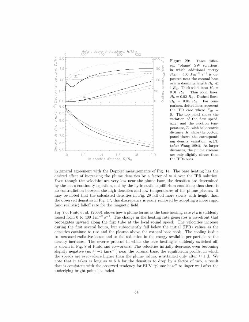
Figure 29: Three differ-ent “plume” SW solutions,in which additional energyFb0 = 400 Jm−2 s−1 is de-posited near the coronal baseover a damping length Hb ≪

1 R⊙. Thick solid lines: Hb =0.01 R⊙. Thin solid lines:Hb = 0.02 R⊙. Dashed lines:Hb = 0.04 R⊙. For com-parison, dotted lines representthe IPR case where Fb0 =0. The top panel shows thevariation of the flow speed,uout, and the electron tem-perature, Te, with heliocentricdistance, R, while the bottompanel shows the correspond-ing density variation, ne(R)(after Wang 1994). At largerdistances, the plume streamsare only slightly slower thanthe IPRs ones.

in general agreement with the Doppler measurements of Fig. 14. The base heating has thedesired effect of increasing the plume densities by a factor of ≈ 4 over the IPR solution.Even though the velocities are very low near the plume base, the densities are determinedby the mass continuity equation, not by the hydrostatic equilibrium condition; thus there isno contradiction between the high densities and low temperatures of the plume plasma. Itmay be noted that the calculated densities in Fig. 29 fall off more slowly with height thanthe observed densities in Fig. 17; this discrepancy is easily removed by adopting a more rapid(and realistic) falloff rate for the magnetic field.

Fig. 7 of Pinto et al. (2009), shows how a plume forms as the base heating rate Fb0 is suddenlyraised from 0 to 400 Jm−2 s−1. The change in the heating rate generates a wavefront thatpropagates upward along the flux tube at the local sound speed. The velocities increaseduring the first several hours, but subsequently fall below the initial (IPR) values as thedensities continue to rise and the plasma above the coronal base cools. The cooling is dueto increased radiative losses and to the reduction in the energy available per particle as thedensity increases. The reverse process, in which the base heating is suddenly switched off,is shown in Fig. 8 of Pinto and co-workers. The velocities initially decrease, even becomingslightly negative (u0 ≈ −1 km s−1) near the coronal base; the equilibrium profile, in whichthe speeds are everywhere higher than the plume values, is attained only after ≈ 1 d. Wenote that it takes as long as ≈ 5 h for the densities to drop by a factor of two, a resultthat is consistent with the observed tendency for EUV “plume haze” to linger well after theunderlying bright point has faded.

54

8.2 Beam and network plumes

Both beam plumes and the individual filaments of network plumes (cf., Sect. 3.2) might havesimilar densities and temperatures; and extend to 1.5 R⊙ to 2.0 R⊙ in VUV images (Gabrielet al. 2009). They are both due to the interaction and reconnection of emerging flux loops(with very different scales) with a monopolar ambient field. Network plumes appear for amaximum of 2 d, due to solar rotation and the evolution time of the network. The individualfilaments of network plumes might have a much shorter lifetime. Jets are characterized by abasic monopole-bipole topology similar to that of plumes, but the energy release is far moreimpulsive, perhaps because the reconnection is driven by the rapid emergence of small bipolesrather than by their slower decay and dispersal in the supergranular flow field.

8.3 Forward modeling

The “forward modeling” approach has been used for many years. The purpose is to obtainsimulated images from controlled parameters with the same statistical characteristics (or atleast the same visual impression) as images of solar coronal plumes. Wang and Sheeley (1995)simulated plumes and their base areas in PCHs, observed in the Mg ix 38.4 nm line with theslitless spectrograph S082A on Skylab. They demonstrated that bright plumes always showintense network features within their base areas, but the converse does not hold. They alsoconsidered how the appearance of UV plumes might depend on their orientation relative to theLOS. From theoretical consideration about the formation of a coronal plume, they deduceda typical time scale τp = 14 h for the energy transfer from the network to the plume.

The purpose of simulations in WL is to reproduce their fluffy aspect in TID, i.e., to mimicin space and time the visual behaviour of plumes, as, for instance, shown in Fig. 30. Twodifferent methods were used by Llebaria et al. (2004) to simulate the image sequences and,from it, the TID. The first one is based on a fractal affine model and the second on anevolutive multi-scale model. These models required both the fractal dimension of 2.9 for the2D electron density distribution over the polar cap. More recently, Boursier and Llebaria(2008) introduced a parametric model based jointly on the “hidden Markov trees” and on the2D wavelet transform, in order to control both the localization of the electrons and the fractaldimension. Simulations of VUV plumes by Barbey et al. (2008) reproduced the intermittentbehaviour of plumes using a dynamic model.

The modeling activities have been successful in the sense that they produce images withrealistic plumes and TID structures and their temporal evolution, although a convincingstatistical comparison between simulation and reality remains to be done.

9 Conclusions

In line with the definition of work in the introduction, ideally answers should be given here toall questions asked in the proposal phase of this study and discussed in the various sections.However, the situation is not ideal: not all problems could be solved and, in some cases, notall team members agreed on a proposed solution. Consequently, three categories will have

55

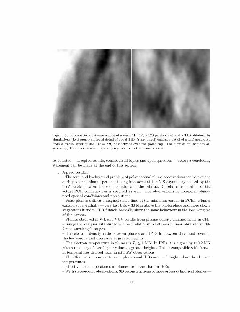
Figure 30: Comparison between a zone of a real TID (128×128 pixels wide) and a TID obtained bysimulation: (Left panel) enlarged detail of a real TID; (right panel) enlarged detail of a TID generatedfrom a fractal distribution (D = 2.9) of electrons over the polar cap. The simulation includes 3Dgeometry, Thompson scattering and projection onto the plane of view.

to be listed—accepted results, controversial topics and open questions—before a concludingstatement can be made at the end of this section.

1. Agreed results:– The fore- and background problem of polar coronal plume observations can be avoidedduring solar minimum periods, taking into account the N-S asymmetry caused by the7.25o angle between the solar equator and the ecliptic. Careful consideration of theactual PCH configuration is required as well. The observations of non-polar plumesneed special conditions and precautions.– Polar plumes delineate magnetic field lines of the minimum corona in PCHs. Plumesexpand super-radially—very fast below 30 Mm above the photosphere and more slowlyat greater altitudes. IPR funnels basically show the same behaviour in the low β-regimeof the corona.– Plumes observed in WL and VUV results from plasma density enhancements in CHs.– Sinogram analyses established a direct relationship between plumes observed in dif-ferent wavelength ranges.– The electron density ratio between plumes and IPRs is between three and seven inthe low corona and decreases at greater heights.– The electron temperature in plumes is Te ≤ 1 MK. In IPRs it is higher by ≈ 0.2 MKwith a tendency of even higher values at greater heights. This is compatible with freeze-in temperatures derived from in situ SW observations.– The effective ion temperatures in plumes and IPRs are much higher than the electrontemperatures.– Effective ion temperatures in plumes are lower than in IPRs.– With stereoscopic observations, 3D reconstructions of more or less cylindrical plumes—

56

called here beam plumes—could be achieved.– Beam plumes are, in many cases, related to coronal BPs during the beginning of theirlifetime that last up to 2 d. They have a recurrence tendency over much longer timescales.– Plumes show some evolution during their lifetime.– Compressional waves are frequently observed in plumes, but these slow magnetosonicwaves do not seem to carry large energy fluxes.– Non-compressional Alfvenic waves are thought to be of importance, at least, in IPRs,but are difficult to detect.– Footpoints of beam plumes lie near magnetic flux concentrations interacting withsmall magnetic dipoles. The reconnection activity generates heat near the base of aplume and leads to jets that probably provide some of the plume plasma.– The SW outflow velocity is higher in IPRs than in plumes above a height of h ≈ 0.6R⊙.The filling factor of plumes in CHs is ≤ 0.1. The IPR contribution to the SW is thusmore important than that of plumes.– Plumes and IPRs have a distinctly different abundance composition, in the sense thatthe ratio of low-FIP/high-FIP elements is much larger in plumes than in IPRs.– Coronal plumes observed in low-latitude CHs have very similar properties to plumesin PCHs.– Rosettes in the chromospheric network could be of importance for the plume forma-tion.– The ensemble of plumes appears to rotate rigidly within the CH boundaries. Thelifetime of a plume is too short for a definite answer.

2. Controversial topics:– Based on EIT observations, a second class of plumes appears to exist. In contrast tobeam plumes, they are composed of small structures—microplumes—with footpointsalong network lanes. They are therefore called network plumes and only visible whenthe LOS is directed in their long dimension.– It is not excluded that beam plumes are also composed of microplumes in a morecompact fashion.– The indication that plumes can be described as fractals support the microplumeconcept.– The outflow speed of the SW at low altitudes is slower in IPRs than in plumes insome studies. Most of the results give, however, higher speeds in IPRs at all heights.– Plume/IPR signatures in the fast SW at large distances from the Sun based oncompositional and magnetic variations appear to be present, but are not sufficientlypronounced for an unambiguous identification.

3. Open questions:– There are indications of temperature anisotropies of heavy ions both in IPRs and inplumes, but the degree of anisotropy in both regions needs further investigations.– Although models of plumes and their formation are available, an exact descriptionof the physical processes operating at the base and inside of plumes as well as theirinteraction with the SW is still outstanding.– Is there any contribution of plume plasma to the fast SW streams at all?– What produces the clear FIP effect signature between plumes and IPRs?

57

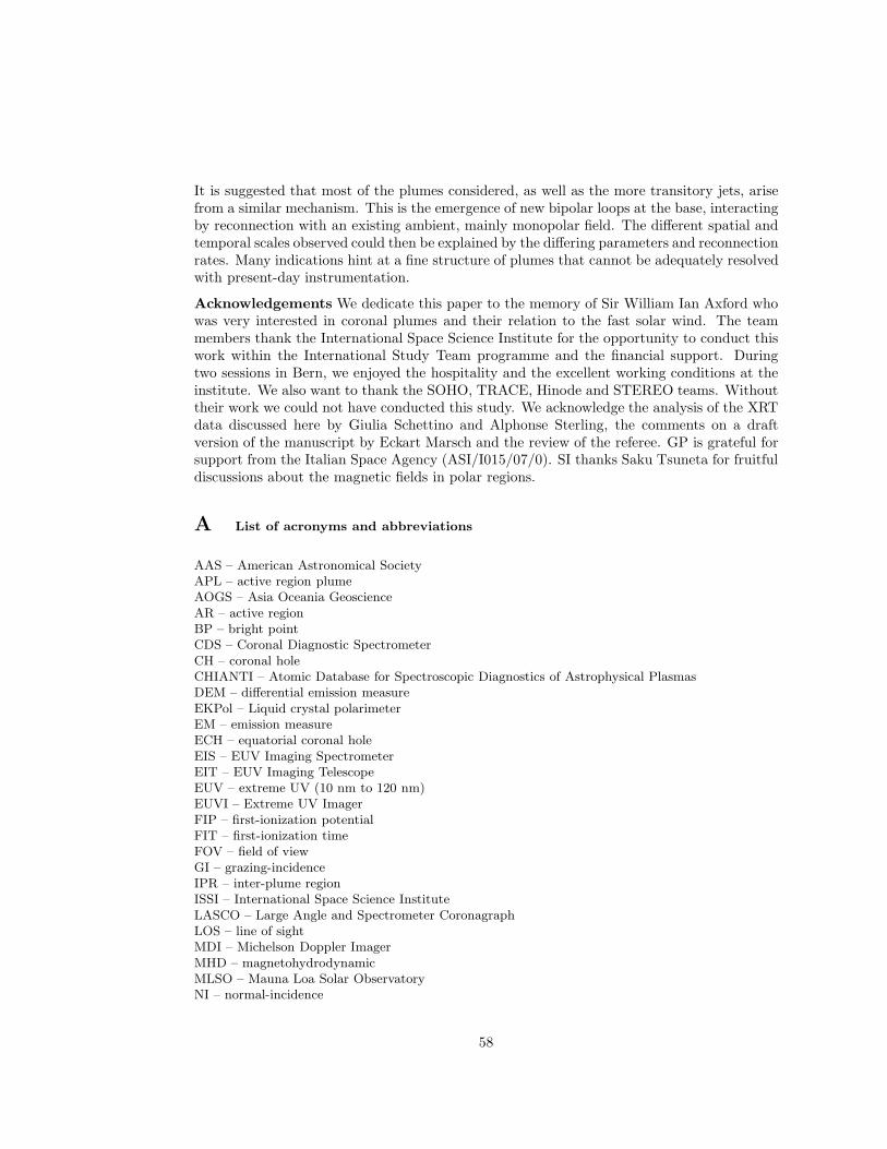
It is suggested that most of the plumes considered, as well as the more transitory jets, arisefrom a similar mechanism. This is the emergence of new bipolar loops at the base, interactingby reconnection with an existing ambient, mainly monopolar field. The different spatial andtemporal scales observed could then be explained by the differing parameters and reconnectionrates. Many indications hint at a fine structure of plumes that cannot be adequately resolvedwith present-day instrumentation.

Acknowledgements We dedicate this paper to the memory of Sir William Ian Axford whowas very interested in coronal plumes and their relation to the fast solar wind. The teammembers thank the International Space Science Institute for the opportunity to conduct thiswork within the International Study Team programme and the financial support. Duringtwo sessions in Bern, we enjoyed the hospitality and the excellent working conditions at theinstitute. We also want to thank the SOHO, TRACE, Hinode and STEREO teams. Withouttheir work we could not have conducted this study. We acknowledge the analysis of the XRTdata discussed here by Giulia Schettino and Alphonse Sterling, the comments on a draftversion of the manuscript by Eckart Marsch and the review of the referee. GP is grateful forsupport from the Italian Space Agency (ASI/I015/07/0). SI thanks Saku Tsuneta for fruitfuldiscussions about the magnetic fields in polar regions.

A List of acronyms and abbreviations

AAS – American Astronomical SocietyAPL – active region plumeAOGS – Asia Oceania GeoscienceAR – active regionBP – bright pointCDS – Coronal Diagnostic SpectrometerCH – coronal holeCHIANTI – Atomic Database for Spectroscopic Diagnostics of Astrophysical PlasmasDEM – differential emission measureEKPol – Liquid crystal polarimeterEM – emission measureECH – equatorial coronal holeEIS – EUV Imaging SpectrometerEIT – EUV Imaging TelescopeEUV – extreme UV (10 nm to 120 nm)EUVI – Extreme UV ImagerFIP – first-ionization potentialFIT – first-ionization timeFOV – field of viewGI – grazing-incidenceIPR – inter-plume regionISSI – International Space Science InstituteLASCO – Large Angle and Spectrometer CoronagraphLOS – line of sightMDI – Michelson Doppler ImagerMHD – magnetohydrodynamicMLSO – Mauna Loa Solar ObservatoryNI – normal-incidence

58

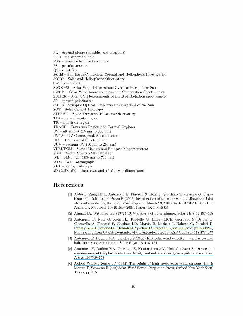
PL – coronal plume (in tables and diagrams)PCH – polar coronal holePBS – pressure-balanced structurePS – pseudostreamerQS – quiet SunSecchi – Sun Earth Connection Coronal and Heliospheric InvestigationSOHO – Solar and Heliospheric ObservatorySW – solar windSWOOPS – Solar Wind Observations Over the Poles of the SunSWICS – Solar Wind Ionization state and Composition SpectrometerSUMER – Solar UV Measurements of Emitted Radiation spectrometerSP – spectro-polarimeterSOLIS – Synoptic Optical Long-term Investigations of the SunSOT – Solar Optical TelescopeSTEREO – Solar Terrestrial Relations ObservatoryTID – time-intensity diagramTR – transition regionTRACE – Transition Region and Coronal ExplorerUV – ultraviolet (10 nm to 380 nm)UVCS – UV Coronagraph SpectrometerUCS – UV Coronal SpectrometerVUV – vacuum UV (10 nm to 200 nm)VHM/FGM – Vector Helium and Fluxgate MagnetometersVSM – Vector Spectro-MagnetographWL – white light (380 nm to 760 nm)WLC – WL CoronagraphXRT – X-Ray Telescope3D (2.5D, 2D) – three-(two and a half, two)-dimensional

References

[1] Abbo L, Zangrilli L, Antonucci E, Fineschi S, Kohl J, Giordano S, Massone G, Capo-bianco G, Calcidese P, Porcu F (2008) Investigation of the solar wind outflows and jointobservations during the total solar eclipse of March 29, 2006. 37th COSPAR ScientificAssembly. Montreal, 13–20 July 2008, Paper: D24-0038-08

[2] Ahmad IA, Withbroe GL (1977) EUV analysis of polar plumes. Solar Phys 53:397–408

[3] Antonucci E, Noci G, Kohl JL, Tondello G, Huber MCE, Giordano S, Benna C,Ciaravella A, Fineschi S, Gardner LD, Martin R, Michels J, Naletto G, Nicolosi P,Panasyuk A, Raymond CJ, Romoli M, Spadaro D, Strachan L, van Ballegooijen A (1997)First results from UVCS: Dynamics of the extended corona. ASP Conf Ser 118:273–277

[4] Antonucci E, Dodero MA, Giordano S (2000) Fast solar wind velocity in a polar coronalhole during solar minimum. Solar Phys 197:115–134

[5] Antonucci E, Dodero MA, Giordano S, Krishnakumar V, Noci G (2004) Spectroscopicmeasurement of the plasma electron density and outflow velocity in a polar coronal hole.A&A 416:749–758

[6] Axford WI, McKenzie JF (1992) The origin of high speed solar wind streams. In: EMarsch E, Schwenn R (eds) Solar Wind Seven, Pergamon Press, Oxford New York SeoulTokyo, pp 1–5

59

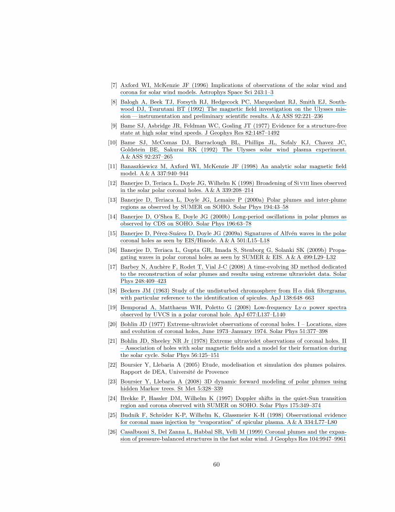
[7] Axford WI, McKenzie JF (1996) Implications of observations of the solar wind andcorona for solar wind models. Astrophys Space Sci 243:1–3

[8] Balogh A, Beek TJ, Forsyth RJ, Hedgecock PC, Marquedant RJ, Smith EJ, South-wood DJ, Tsurutani BT (1992) The magnetic field investigation on the Ulysses mis-sion— instrumentation and preliminary scientific results. A&ASS 92:221–236

[9] Bame SJ, Asbridge JR, Feldman WC, Gosling JT (1977) Evidence for a structure-freestate at high solar wind speeds. J Geophys Res 82:1487–1492

[10] Bame SJ, McComas DJ, Barraclough BL, Phillips JL, Sofaly KJ, Chavez JC,Goldstein BE, Sakurai RK (1992) The Ulysses solar wind plasma experiment.A&ASS 92:237–265

[11] Banaszkiewicz M, Axford WI, McKenzie JF (1998) An analytic solar magnetic fieldmodel. A&A 337:940–944

[12] Banerjee D, Teriaca L, Doyle JG, Wilhelm K (1998) Broadening of Siviii lines observedin the solar polar coronal holes. A&A 339:208–214

[13] Banerjee D, Teriaca L, Doyle JG, Lemaire P (2000a) Polar plumes and inter-plumeregions as observed by SUMER on SOHO. Solar Phys 194:43–58

[14] Banerjee D, O’Shea E, Doyle JG (2000b) Long-period oscillations in polar plumes asobserved by CDS on SOHO. Solar Phys 196:63–78

[15] Banerjee D, Perez-Suarez D, Doyle JG (2009a) Signatures of Alfven waves in the polarcoronal holes as seen by EIS/Hinode. A&A 501:L15–L18

[16] Banerjee D, Teriaca L, Gupta GR, Imada S, Stenborg G, Solanki SK (2009b) Propa-gating waves in polar coronal holes as seen by SUMER & EIS. A&A 499:L29–L32

[17] Barbey N, Auchere F, Rodet T, Vial J-C (2008) A time-evolving 3D method dedicatedto the reconstruction of solar plumes and results using extreme ultraviolet data. SolarPhys 248:409–423

[18] Beckers JM (1963) Study of the undisturbed chromosphere from Hα disk filtergrams,with particular reference to the identification of spicules. ApJ 138:648–663

[19] Bemporad A, Matthaeus WH, Poletto G (2008) Low-frequency Lyα power spectraobserved by UVCS in a polar coronal hole. ApJ 677:L137–L140

[20] Bohlin JD (1977) Extreme-ultraviolet observations of coronal holes. I – Locations, sizesand evolution of coronal holes, June 1973–January 1974. Solar Phys 51:377–398

[21] Bohlin JD, Sheeley NR Jr (1978) Extreme ultraviolet observations of coronal holes. II– Association of holes with solar magnetic fields and a model for their formation duringthe solar cycle. Solar Phys 56:125–151

[22] Boursier Y, Llebaria A (2005) Etude, modelisation et simulation des plumes polaires.Rapport de DEA, Universite de Provence

[23] Boursier Y, Llebaria A (2008) 3D dynamic forward modeling of polar plumes usinghidden Markov trees. St Met 5:328–339

[24] Brekke P, Hassler DM, Wilhelm K (1997) Doppler shifts in the quiet-Sun transitionregion and corona observed with SUMER on SOHO. Solar Phys 175:349–374

[25] Budnik F, Schroder K-P, Wilhelm K, Glassmeier K-H (1998) Observational evidencefor coronal mass injection by “evaporation” of spicular plasma. A&A 334:L77–L80

[26] Casalbuoni S, Del Zanna L, Habbal SR, Velli M (1999) Coronal plumes and the expan-sion of pressure-balanced structures in the fast solar wind. J Geophys Res 104:9947–9961

60

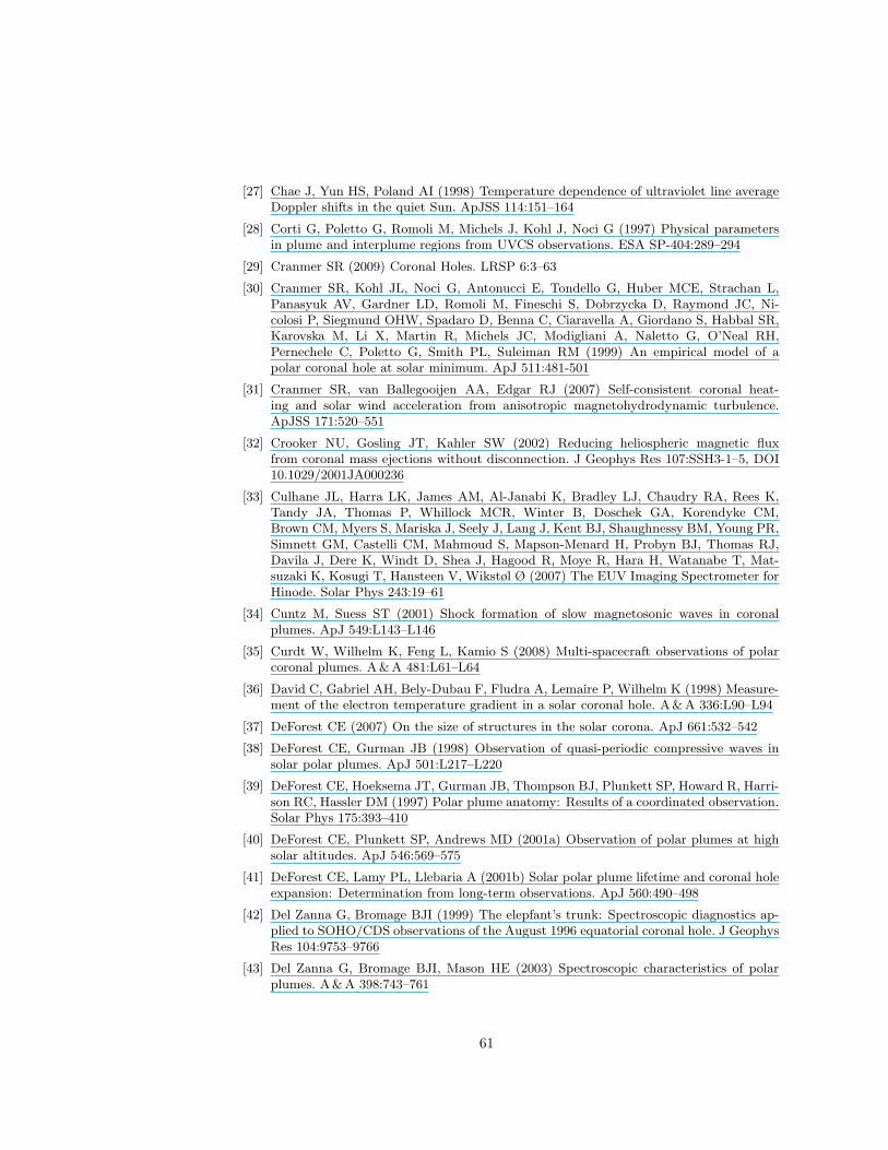
[27] Chae J, Yun HS, Poland AI (1998) Temperature dependence of ultraviolet line averageDoppler shifts in the quiet Sun. ApJSS 114:151–164

[28] Corti G, Poletto G, Romoli M, Michels J, Kohl J, Noci G (1997) Physical parametersin plume and interplume regions from UVCS observations. ESA SP-404:289–294

[29] Cranmer SR (2009) Coronal Holes. LRSP 6:3–63

[30] Cranmer SR, Kohl JL, Noci G, Antonucci E, Tondello G, Huber MCE, Strachan L,Panasyuk AV, Gardner LD, Romoli M, Fineschi S, Dobrzycka D, Raymond JC, Ni-colosi P, Siegmund OHW, Spadaro D, Benna C, Ciaravella A, Giordano S, Habbal SR,Karovska M, Li X, Martin R, Michels JC, Modigliani A, Naletto G, O’Neal RH,Pernechele C, Poletto G, Smith PL, Suleiman RM (1999) An empirical model of apolar coronal hole at solar minimum. ApJ 511:481-501

[31] Cranmer SR, van Ballegooijen AA, Edgar RJ (2007) Self-consistent coronal heat-ing and solar wind acceleration from anisotropic magnetohydrodynamic turbulence.ApJSS 171:520–551

[32] Crooker NU, Gosling JT, Kahler SW (2002) Reducing heliospheric magnetic fluxfrom coronal mass ejections without disconnection. J Geophys Res 107:SSH3-1–5, DOI10.1029/2001JA000236

[33] Culhane JL, Harra LK, James AM, Al-Janabi K, Bradley LJ, Chaudry RA, Rees K,Tandy JA, Thomas P, Whillock MCR, Winter B, Doschek GA, Korendyke CM,Brown CM, Myers S, Mariska J, Seely J, Lang J, Kent BJ, Shaughnessy BM, Young PR,Simnett GM, Castelli CM, Mahmoud S, Mapson-Menard H, Probyn BJ, Thomas RJ,Davila J, Dere K, Windt D, Shea J, Hagood R, Moye R, Hara H, Watanabe T, Mat-suzaki K, Kosugi T, Hansteen V, Wikstøl Ø (2007) The EUV Imaging Spectrometer forHinode. Solar Phys 243:19–61

[34] Cuntz M, Suess ST (2001) Shock formation of slow magnetosonic waves in coronalplumes. ApJ 549:L143–L146

[35] Curdt W, Wilhelm K, Feng L, Kamio S (2008) Multi-spacecraft observations of polarcoronal plumes. A&A 481:L61–L64

[36] David C, Gabriel AH, Bely-Dubau F, Fludra A, Lemaire P, Wilhelm K (1998) Measure-ment of the electron temperature gradient in a solar coronal hole. A&A 336:L90–L94

[37] DeForest CE (2007) On the size of structures in the solar corona. ApJ 661:532–542

[38] DeForest CE, Gurman JB (1998) Observation of quasi-periodic compressive waves insolar polar plumes. ApJ 501:L217–L220

[39] DeForest CE, Hoeksema JT, Gurman JB, Thompson BJ, Plunkett SP, Howard R, Harri-son RC, Hassler DM (1997) Polar plume anatomy: Results of a coordinated observation.Solar Phys 175:393–410

[40] DeForest CE, Plunkett SP, Andrews MD (2001a) Observation of polar plumes at highsolar altitudes. ApJ 546:569–575

[41] DeForest CE, Lamy PL, Llebaria A (2001b) Solar polar plume lifetime and coronal holeexpansion: Determination from long-term observations. ApJ 560:490–498

[42] Del Zanna G, Bromage BJI (1999) The elepfant’s trunk: Spectroscopic diagnostics ap-plied to SOHO/CDS observations of the August 1996 equatorial coronal hole. J GeophysRes 104:9753–9766

[43] Del Zanna G, Bromage BJI, Mason HE (2003) Spectroscopic characteristics of polarplumes. A&A 398:743–761

61

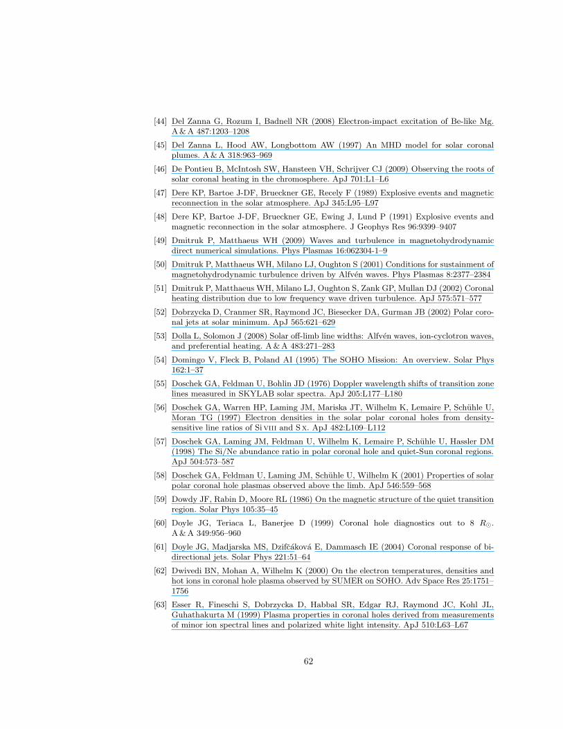
[44] Del Zanna G, Rozum I, Badnell NR (2008) Electron-impact excitation of Be-like Mg.A&A 487:1203–1208

[45] Del Zanna L, Hood AW, Longbottom AW (1997) An MHD model for solar coronalplumes. A&A 318:963–969

[46] De Pontieu B, McIntosh SW, Hansteen VH, Schrijver CJ (2009) Observing the roots ofsolar coronal heating in the chromosphere. ApJ 701:L1–L6

[47] Dere KP, Bartoe J-DF, Brueckner GE, Recely F (1989) Explosive events and magneticreconnection in the solar atmosphere. ApJ 345:L95–L97

[48] Dere KP, Bartoe J-DF, Brueckner GE, Ewing J, Lund P (1991) Explosive events andmagnetic reconnection in the solar atmosphere. J Geophys Res 96:9399–9407

[49] Dmitruk P, Matthaeus WH (2009) Waves and turbulence in magnetohydrodynamicdirect numerical simulations. Phys Plasmas 16:062304-1–9

[50] Dmitruk P, Matthaeus WH, Milano LJ, Oughton S (2001) Conditions for sustainment ofmagnetohydrodynamic turbulence driven by Alfven waves. Phys Plasmas 8:2377–2384

[51] Dmitruk P, Matthaeus WH, Milano LJ, Oughton S, Zank GP, Mullan DJ (2002) Coronalheating distribution due to low frequency wave driven turbulence. ApJ 575:571–577

[52] Dobrzycka D, Cranmer SR, Raymond JC, Biesecker DA, Gurman JB (2002) Polar coro-nal jets at solar minimum. ApJ 565:621–629

[53] Dolla L, Solomon J (2008) Solar off-limb line widths: Alfven waves, ion-cyclotron waves,and preferential heating. A&A 483:271–283

[54] Domingo V, Fleck B, Poland AI (1995) The SOHO Mission: An overview. Solar Phys162:1–37

[55] Doschek GA, Feldman U, Bohlin JD (1976) Doppler wavelength shifts of transition zonelines measured in SKYLAB solar spectra. ApJ 205:L177–L180

[56] Doschek GA, Warren HP, Laming JM, Mariska JT, Wilhelm K, Lemaire P, Schuhle U,Moran TG (1997) Electron densities in the solar polar coronal holes from density-sensitive line ratios of Siviii and Sx. ApJ 482:L109–L112

[57] Doschek GA, Laming JM, Feldman U, Wilhelm K, Lemaire P, Schuhle U, Hassler DM(1998) The Si/Ne abundance ratio in polar coronal hole and quiet-Sun coronal regions.ApJ 504:573–587

[58] Doschek GA, Feldman U, Laming JM, Schuhle U, Wilhelm K (2001) Properties of solarpolar coronal hole plasmas observed above the limb. ApJ 546:559–568

[59] Dowdy JF, Rabin D, Moore RL (1986) On the magnetic structure of the quiet transitionregion. Solar Phys 105:35–45

[60] Doyle JG, Teriaca L, Banerjee D (1999) Coronal hole diagnostics out to 8 R⊙.A&A 349:956–960

[61] Doyle JG, Madjarska MS, Dzifcakova E, Dammasch IE (2004) Coronal response of bi-directional jets. Solar Phys 221:51–64

[62] Dwivedi BN, Mohan A, Wilhelm K (2000) On the electron temperatures, densities andhot ions in coronal hole plasma observed by SUMER on SOHO. Adv Space Res 25:1751–1756

[63] Esser R, Fineschi S, Dobrzycka D, Habbal SR, Edgar RJ, Raymond JC, Kohl JL,Guhathakurta M (1999) Plasma properties in coronal holes derived from measurementsof minor ion spectral lines and polarized white light intensity. ApJ 510:L63–L67

62

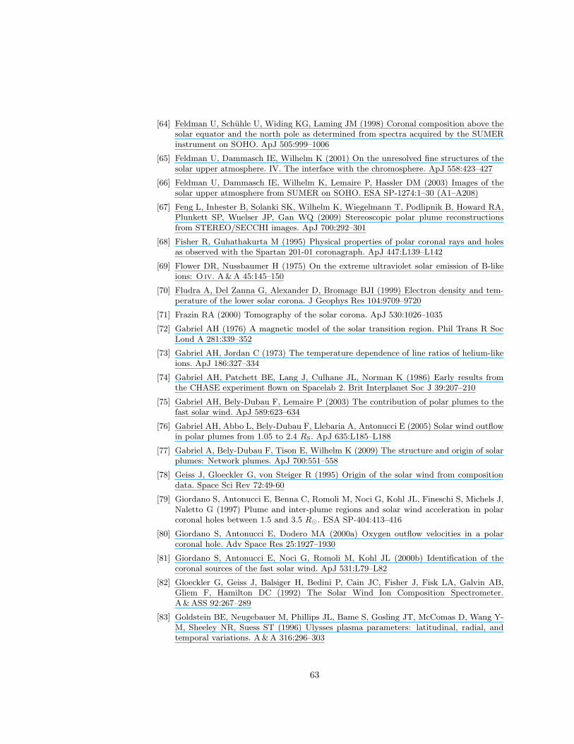
[64] Feldman U, Schuhle U, Widing KG, Laming JM (1998) Coronal composition above thesolar equator and the north pole as determined from spectra acquired by the SUMERinstrument on SOHO. ApJ 505:999–1006

[65] Feldman U, Dammasch IE, Wilhelm K (2001) On the unresolved fine structures of thesolar upper atmosphere. IV. The interface with the chromosphere. ApJ 558:423–427

[66] Feldman U, Dammasch IE, Wilhelm K, Lemaire P, Hassler DM (2003) Images of thesolar upper atmosphere from SUMER on SOHO. ESA SP-1274:1–30 (A1–A208)

[67] Feng L, Inhester B, Solanki SK, Wilhelm K, Wiegelmann T, Podlipnik B, Howard RA,Plunkett SP, Wuelser JP, Gan WQ (2009) Stereoscopic polar plume reconstructionsfrom STEREO/SECCHI images. ApJ 700:292–301

[68] Fisher R, Guhathakurta M (1995) Physical properties of polar coronal rays and holesas observed with the Spartan 201-01 coronagraph. ApJ 447:L139–L142

[69] Flower DR, Nussbaumer H (1975) On the extreme ultraviolet solar emission of B-likeions: O iv. A&A 45:145–150

[70] Fludra A, Del Zanna G, Alexander D, Bromage BJI (1999) Electron density and tem-perature of the lower solar corona. J Geophys Res 104:9709–9720

[71] Frazin RA (2000) Tomography of the solar corona. ApJ 530:1026–1035

[72] Gabriel AH (1976) A magnetic model of the solar transition region. Phil Trans R SocLond A 281:339–352

[73] Gabriel AH, Jordan C (1973) The temperature dependence of line ratios of helium-likeions. ApJ 186:327–334

[74] Gabriel AH, Patchett BE, Lang J, Culhane JL, Norman K (1986) Early results fromthe CHASE experiment flown on Spacelab 2. Brit Interplanet Soc J 39:207–210

[75] Gabriel AH, Bely-Dubau F, Lemaire P (2003) The contribution of polar plumes to thefast solar wind. ApJ 589:623–634

[76] Gabriel AH, Abbo L, Bely-Dubau F, Llebaria A, Antonucci E (2005) Solar wind outflowin polar plumes from 1.05 to 2.4 RS. ApJ 635:L185–L188

[77] Gabriel A, Bely-Dubau F, Tison E, Wilhelm K (2009) The structure and origin of solarplumes: Network plumes. ApJ 700:551–558

[78] Geiss J, Gloeckler G, von Steiger R (1995) Origin of the solar wind from compositiondata. Space Sci Rev 72:49-60

[79] Giordano S, Antonucci E, Benna C, Romoli M, Noci G, Kohl JL, Fineschi S, Michels J,Naletto G (1997) Plume and inter-plume regions and solar wind acceleration in polarcoronal holes between 1.5 and 3.5 R⊙. ESA SP-404:413–416

[80] Giordano S, Antonucci E, Dodero MA (2000a) Oxygen outflow velocities in a polarcoronal hole. Adv Space Res 25:1927–1930

[81] Giordano S, Antonucci E, Noci G, Romoli M, Kohl JL (2000b) Identification of thecoronal sources of the fast solar wind. ApJ 531:L79–L82

[82] Gloeckler G, Geiss J, Balsiger H, Bedini P, Cain JC, Fisher J, Fisk LA, Galvin AB,Gliem F, Hamilton DC (1992) The Solar Wind Ion Composition Spectrometer.A&ASS 92:267–289

[83] Goldstein BE, Neugebauer M, Phillips JL, Bame S, Gosling JT, McComas D, Wang Y-M, Sheeley NR, Suess ST (1996) Ulysses plasma parameters: latitudinal, radial, andtemporal variations. A&A 316:296–303

63

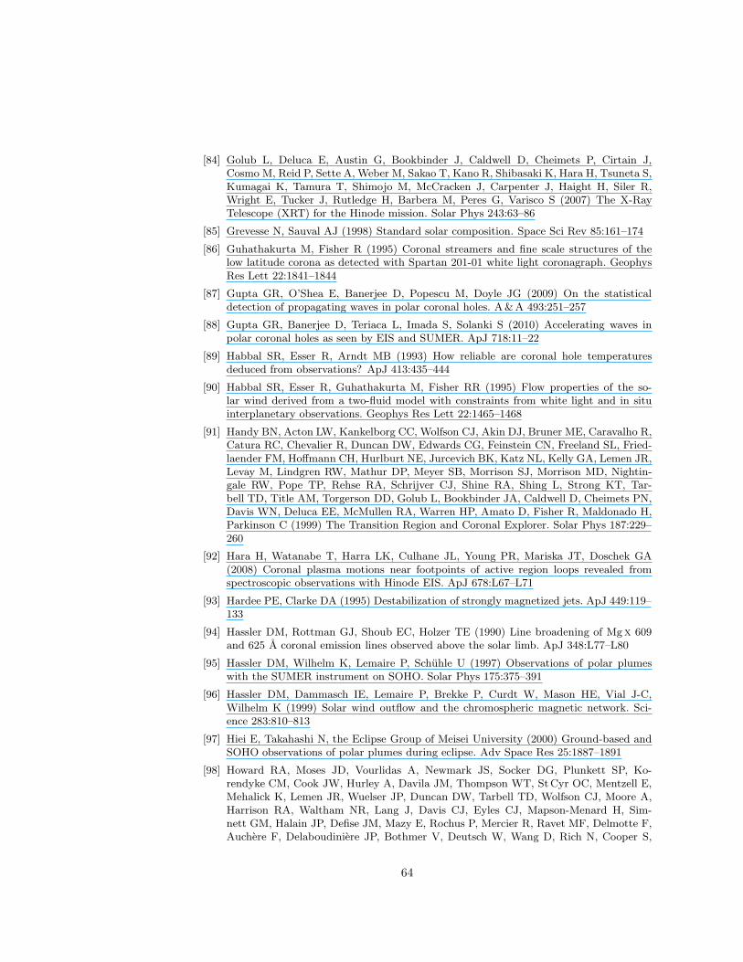
[84] Golub L, Deluca E, Austin G, Bookbinder J, Caldwell D, Cheimets P, Cirtain J,Cosmo M, Reid P, Sette A, Weber M, Sakao T, Kano R, Shibasaki K, Hara H, Tsuneta S,Kumagai K, Tamura T, Shimojo M, McCracken J, Carpenter J, Haight H, Siler R,Wright E, Tucker J, Rutledge H, Barbera M, Peres G, Varisco S (2007) The X-RayTelescope (XRT) for the Hinode mission. Solar Phys 243:63–86

[85] Grevesse N, Sauval AJ (1998) Standard solar composition. Space Sci Rev 85:161–174

[86] Guhathakurta M, Fisher R (1995) Coronal streamers and fine scale structures of thelow latitude corona as detected with Spartan 201-01 white light coronagraph. GeophysRes Lett 22:1841–1844

[87] Gupta GR, O’Shea E, Banerjee D, Popescu M, Doyle JG (2009) On the statisticaldetection of propagating waves in polar coronal holes. A&A 493:251–257

[88] Gupta GR, Banerjee D, Teriaca L, Imada S, Solanki S (2010) Accelerating waves inpolar coronal holes as seen by EIS and SUMER. ApJ 718:11–22

[89] Habbal SR, Esser R, Arndt MB (1993) How reliable are coronal hole temperaturesdeduced from observations? ApJ 413:435–444

[90] Habbal SR, Esser R, Guhathakurta M, Fisher RR (1995) Flow properties of the so-lar wind derived from a two-fluid model with constraints from white light and in situinterplanetary observations. Geophys Res Lett 22:1465–1468

[91] Handy BN, Acton LW, Kankelborg CC, Wolfson CJ, Akin DJ, Bruner ME, Caravalho R,Catura RC, Chevalier R, Duncan DW, Edwards CG, Feinstein CN, Freeland SL, Fried-laender FM, Hoffmann CH, Hurlburt NE, Jurcevich BK, Katz NL, Kelly GA, Lemen JR,Levay M, Lindgren RW, Mathur DP, Meyer SB, Morrison SJ, Morrison MD, Nightin-gale RW, Pope TP, Rehse RA, Schrijver CJ, Shine RA, Shing L, Strong KT, Tar-bell TD, Title AM, Torgerson DD, Golub L, Bookbinder JA, Caldwell D, Cheimets PN,Davis WN, Deluca EE, McMullen RA, Warren HP, Amato D, Fisher R, Maldonado H,Parkinson C (1999) The Transition Region and Coronal Explorer. Solar Phys 187:229–260

[92] Hara H, Watanabe T, Harra LK, Culhane JL, Young PR, Mariska JT, Doschek GA(2008) Coronal plasma motions near footpoints of active region loops revealed fromspectroscopic observations with Hinode EIS. ApJ 678:L67–L71

[93] Hardee PE, Clarke DA (1995) Destabilization of strongly magnetized jets. ApJ 449:119–133

[94] Hassler DM, Rottman GJ, Shoub EC, Holzer TE (1990) Line broadening of Mgx 609and 625 A coronal emission lines observed above the solar limb. ApJ 348:L77–L80

[95] Hassler DM, Wilhelm K, Lemaire P, Schuhle U (1997) Observations of polar plumeswith the SUMER instrument on SOHO. Solar Phys 175:375–391

[96] Hassler DM, Dammasch IE, Lemaire P, Brekke P, Curdt W, Mason HE, Vial J-C,Wilhelm K (1999) Solar wind outflow and the chromospheric magnetic network. Sci-ence 283:810–813

[97] Hiei E, Takahashi N, the Eclipse Group of Meisei University (2000) Ground-based andSOHO observations of polar plumes during eclipse. Adv Space Res 25:1887–1891

[98] Howard RA, Moses JD, Vourlidas A, Newmark JS, Socker DG, Plunkett SP, Ko-rendyke CM, Cook JW, Hurley A, Davila JM, Thompson WT, StCyr OC, Mentzell E,Mehalick K, Lemen JR, Wuelser JP, Duncan DW, Tarbell TD, Wolfson CJ, Moore A,Harrison RA, Waltham NR, Lang J, Davis CJ, Eyles CJ, Mapson-Menard H, Sim-nett GM, Halain JP, Defise JM, Mazy E, Rochus P, Mercier R, Ravet MF, Delmotte F,Auchere F, Delaboudiniere JP, Bothmer V, Deutsch W, Wang D, Rich N, Cooper S,

64

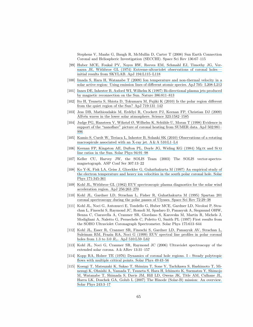
Stephens V, Maahs G, Baugh R, McMullin D, Carter T (2008) Sun Earth ConnectionCoronal and Heliospheric Investigation (SECCHI). Space Sci Rev 136:67–115

[99] Huber MCE, Foukal PV, Noyes RW, Reeves EM, Schmahl EJ, Timothy JG, Ver-nazza JE, Withbroe GL (1974) Extreme-ultraviolet observations of coronal holes—initial results from SKYLAB. ApJ 194:L115–L118

[100] Imada S, Hara H, Watanabe T (2009) Ion temperature and non-thermal velocity in asolar active region: Using emission lines of different atomic species. ApJ 705: L208-L212

[101] Innes DE, Inhester B, Axford WI, Wilhelm K (1997) Bi-directional plasma jets producedby magnetic reconnection on the Sun. Nature 386:811–813

[102] Ito H, Tsuneta S, Shiota D, Tokumaru M, Fujiki K (2010) Is the polar region differentfrom the quiet region of the Sun? ApJ 719:131–142

[103] Jess DB, Mathioudakis M, Erdelyi R, Crockett PJ, Keenan FP, Christian DJ (2009)Alfven waves in the lower solar atmosphere. Science 323:1582–1585

[104] Judge PG, Hansteen V, Wikstøl Ø, Wilhelm K, Schuhle U, Moran T (1998) Evidence insupport of the “nanoflare” picture of coronal heating from SUMER data. ApJ 502:981–996

[105] Kamio S, Curdt W, Teriaca L, Inhester B, Solanki SK (2010) Observations of a rotatingmacrospicule associated with an X-ray jet. A&A 510:L1–L4

[106] Keenan FP, Kingston AE, Dufton PL, Doyle JG, Widing KG (1984) Mg ix and Sixiline ratios in the Sun. Solar Phys 94:91–98

[107] Keller CU, Harvey JW, the SOLIS Team (2003) The SOLIS vector-spectro-magnetograph. ASP Conf Ser 307:13–22

[108] Ko Y-K, Fisk LA, Geiss J, Gloeckler G, Guhathakurta M (1997) An empirical study ofthe electron temperature and heavy ion velocities in the south polar coronal hole. SolarPhys 171:345-361

[109] Kohl JL, Withbroe GL (1982) EUV spectroscopic plasma diagnostics for the solar windacceleration region. ApJ 256:263–270

[110] Kohl JL, Gardner LD, Strachan L, Fisher R, Guhathakurta M (1995) Spartan 201coronal spectroscopy during the polar passes of Ulysses. Space Sci Rev 72:29–38

[111] Kohl JL, Noci G, Antonucci E, Tondello G, Huber MCE, Gardner LD, Nicolosi P, Stra-chan L, Fineschi S, Raymond JC, Romoli M, Spadaro D, Panasyuk A, Siegmund OHW,Benna C, Ciaravella A, Cranmer SR, Giordano S, Karovska M, Martin R, Michels J,Modigliani A, Naletto G, Pernechele C, Poletto G, Smith PL (1997) First results fromthe SOHO Ultraviolet Coronagraph Spectrometer. Solar Phys 175:613–644

[112] Kohl JL, Esser R, Cranmer SR, Fineschi S, Gardner LD, Panasyuk AV, Strachan L,Suleiman RM, Frazin RA, Noci G (1999) EUV spectral line profiles in polar coronalholes from 1.3 to 3.0 R⊙. ApJ 510:L59–L62

[113] Kohl JL, Noci G, Cranmer SR, Raymond JC (2006) Ultraviolet spectroscopy of theextended solar corona. A&ARev 13:31–157

[114] Kopp RA, Holzer TE (1976) Dynamics of coronal hole regions. I - Steady polytropicflows with multiple critical points. Solar Phys 49:43–56

[115] Kosugi T, Matsuzaki K, Sakao T, Shimizu T, Sone Y, Tachikawa S, Hashimoto T, Mi-nesugi K, Ohnishi A, Yamada T, Tsuneta S, Hara H, Ichimoto K, Suematsu Y, ShimojoM, Watanabe T, Shimada S, Davis JM, Hill LD, Owens JK, Title AM, Culhane JL,Harra LK, Doschek GA, Golub L (2007) The Hinode (Solar-B) mission: An overview.Solar Phys 243:3–17

65

[116] Koutchmy S (1977) Study of the June 30, 1973 trans-polar coronal hole. SolarPhys 51:399-407

[117] Koutchmy S (1994) Coronal physics from eclipse observations. Adv Space Res 14:(4)29–39

[118] Koutchmy S, Bocchialini K (1998) White-light polar plumes from solar eclipses. ESASP-421:51–62

[119] Koutchmy S, Daniel J-Y, Mouette J, Vilinga J, Noens J-C, Dame L, Faurobert M,Dara H, Hady A, Semeida M, Sabry M, Domenech, A, Munier J-M, Jimenez R, LegaultTh, Viladrich Ch, Kuzin S, Pertsov A, the O.A. Team (2006) Preliminary results fromthe March 29, 2006 total eclipse observations in Egypt. Proc Annual Meeting Soc Fran-caise Astron Astrophys, 547–548

[120] Krieger AS, Timothy AF, Roelof EC (1973) A coronal hole and its identification as thesource of a high velocity solar wind stream. Solar Phys 29:505–525

[121] Laming JM, Feldman U (2001) The solar helium abundance in the outer corona deter-mined from observations with SUMER/SOHO. ApJ 546:552–559

[122] Laming JM, Feldman U, Schuhle U, Lemaire P, Curdt W, Wilhelm K (1997) Elec-tron density diagnostics for the solar upper atmosphere from spectra obtained bySUMER/SOHO. ApJ 485:911–919

[123] Lamy P, Llebaria A, Koutchmy S, Reynet P, Molodensky M, Howard R, Schwenn R,Simnett G (1997) Characterization of polar plumes from LASCO-C2 images in early1996. ESA SP-404:487–490

[124] Landi E (2008) The off-disk thermal structure of a polar coronal hole. ApJ 685:1270–1276

[125] Landi E, Feldman U, Doschek GA (2007) Neon and oxygen absolute abundances in thesolar corona. ApJ 659:743–749

[126] Lites BW, Card G, Elmore DF, Holzer T, Lecinski A, Streander KV, Tomczyk S, Gur-man JB (1999) Dynamics of polar plumes observed at the 1998 February 26 eclipse.Solar Phys 190:185–206

[127] Llebaria A, Lamy P, DeForest CE, Koutchmy S (1998) Time domain analysis of polarplumes observed with LASCO-C2 and EIT. ESA SP-421:87–92

[128] Llebaria A, Thernisien A, Lamy P (2001) Projective transform techniques to recon-struct the 3-D structure and the temporal evolution of solar polar plumes. ASP ConfSer 238:377–380

[129] Llebaria A, Saez F, Lamy P (2002a) The fractal nature of the polar plumes. ESA SP-508:391–394

[130] Llebaria A, Thernisien A, Lamy P (2002b) Characterization of the polar plumes fromhigh cadence LASCO-C2 observations. Adv Space Res 29:343–348

[131] Llebaria A, Boulanger J, Boursier Y (2004) Time domain analysis of polar plumesobserved with the LASCO/SOHO coronagraph. Proc ADA-III, Astron Data AnalysisConf, eWIC Conf (http://www.bcs.org/server.php?show=conWebDoc.3885)

[132] Llebaria A, Loirat J, Lamy P (2010) Restitution of multiple overlaid components onextremely long series of solar corona images. SPIE Proc 7533:0Y-1–8

[133] Madjarska MS, Doyle JG, Teriaca L, Banerjee D (2003) An EUV bright point as seenby SUMER, CDS, MDI and EIT on-board SOHO. A&A 398:775–784

[134] Mariska JT (1992) The solar transition region. Cambridge University Press, Cambridge

66

[135] Marsch E, Tu C-Y (1997) Solar wind and chromospheric network. Solar Phys 176:87–106.

[136] Marsch E, Tu C-Y, Wilhelm K, Curdt W, Schuhle U, Dammasch IE (1997) Brightplumes and dark lanes as observed in Mgx 625 A and Nv 1239 A in the solar polarcorona. ESA SP-404:555–560

[137] Mason HE, Young PR, Pike CD, Harrison RA, Fludra A, Bromage BJI, Del Zanna G(1997) Application of spectroscopic diagnostics to early observations with the SOHOCoronal Diagnostic Spectrometer. Solar Phys 170:143–161

[138] Matthaeus WH, Goldstein ML (1986) Low-frequency 1/f noise in the interplanetarymagnetic field. Phys Rev Lett 57:495–498

[139] Matthaeus WH, Zank GP, Oughton S, Mullan DJ, Dmitruk P (1999) Coronal heat-ing by magnetohydrodynamic turbulence driven by reflected low-frequency waves.ApJ 523:L93–L96

[140] Matthaeus WH, Breech B, Dmitruk P, Bemporad A, Poletto G, Velli M, Romoli M(2007) Density and magnetic field signatures of interplanetary 1/f noise. ApJ 657:L121–L124

[141] Mazzotta P, Mazzitelli G, Colafrancesco S, Vittorio N (1998) Ionization balance foroptically thin plasmas: Rate coefficients for all atoms and ions of the elements H to Ni.A&ASS 133:403–409

[142] McKenzie JF, Banaszkiewicz M, Axford WI (1995) Acceleration of the high speed solarwind. A&A 303:L45–L48

[143] Miralles MP, Cranmer SR, Kohl JL (2001) Ultraviolet Coronagraph Spectrometer ob-servations of a high-latitude coronal hole with high oxygen temperatures and the nextsolar cycle polarity. ApJ 560:L193–L196

[144] Moran T, Gopalswamy N, Dammasch IE, Wilhelm K (2001) A multi-wavelength studyof solar coronal-hole regions showing radio enhancements. A&A 378:1037–1045

[145] Moses D, Clette F, Delaboudiniere J-P, Artzner GE, Bougnet M, Brunaud J, Cara-betian C, Gabriel AH, Hochedez JF, Millier F, Song XY, Au B, Dere KP, Howard RA,Kreplin R, Michels DJ, Defise JM, Jamar C, Rochus P, Chauvineau JP, Marioge JP,Catura RC, Lemen JR, Shing L, Stern RA, Gurman JB, Neupert WM, Newmark J,Thompson B, Maucherat A, Portier-Fozzani F, Berghmans D, Cugnon P, van Dessel EL,Gabryl JR (1997) EIT observations of the extreme ultraviolet Sun. Solar Phys 175:571–599

[146] Munro RH, Jackson BV (1977) Physical properties of a coronal hole from 2 to 5 R⊙.ApJ 213:874–886

[147] Neugebauer M, Goldstein BE, McComas DJ, Suess ST, Balogh A (1995) Ulysses obser-vations of microstreams in the solar wind from coronal holes. J Geophys Res 100:23 389–23 395

[148] Newkirk G Jr, Harvey J (1968) Coronal polar plumes. Solar Phys 3:321–343

[149] Noci G, Kohl JL, Withbroe GL (1987) Solar wind diagnostics from Doppler-enhancedscattering. ApJ 315:706–715.

[150] November LJ, Koutchmy S (1996) White-light coronal dark threads and density finestructure. ApJ 466:512–528

[151] Ofman L (2005) MHD waves and heating in coronal holes. Space Sci Rev 120:67–94

[152] Ofman L, Davila JM (1995) Alfven wave heating of coronal holes and the relation tothe high-speed solar wind. J Geophys Res 100:23 413–23 425

67

[153] Ofman L, Romoli M, Poletto G, Noci G, Kohl JL (1997) Ultraviolet Coronagraph Spec-trometer observations of density fluctuations in the solar wind. ApJ 491:L111–L114

[154] Ofman L, Nakariakov VM, DeForest CE (1999) Slow magnetosonic waves in coronalplumes. ApJ 514:441–447

[155] Ofman L, Romoli M, Poletto G, Noci G, Kohl JL (2000a) UVCS WLC observations ofcompressional waves in the south polar coronal hole. ApJ 529:592–598

[156] Ofman L, Nakariakov VM, Sehgal N (2000b) Dissipation of slow magnetosonic waves incoronal plumes. ApJ 533:1071–1083

[157] Parhi S, Suess ST, Sulkanen M (1999) Can Kelvin–Helmholtz instabilities of jet-likestructures and plumes cause solar wind fluctuations at 1 AU? J Geophys Res 104:14 781–14 787

[158] Parker EN (1988) Nanoflares and the solar X-ray corona. ApJ 330:474–479

[159] Pasachoff JM, Rusin V, Druckmuller M, Druckmullerova, H, Belık M, Saniga M, Mi-narovjech M, Markova E, Babcock BA, Souza SP, Levitt JS (2008) Polar plume bright-ening during the 2006 March 29 total eclipse. ApJ 682:638–643

[160] Pasachoff JM, Rusin V, Druckmuller M, Aniol P, Saniga M, Minarovjech M (2009) The2008 August 1 eclipse solar-minimum corona unraveled. ApJ 702:1297–1308

[161] Patsourakos S, Vial J-C (2000) Outflow velocity of interplume regions at the base ofpolar coronal holes. A&A 359:L1–L4

[162] Phillips KJH, Sylwester J, Sylwester B, Landi E (2003) Solar flare abundances of potas-sium, argon, and sulphur. ApJ 589:L113–L116

[163] Pinto R, Grappin R, Wang Y-M, Leorat J (2009) Time-dependent hydrodynamicalsimulations of slow solar wind, coronal inflows, and polar plumes. A&A 497:537–543

[164] Pinto R, Grappin R, Leorat J(2010) Coronal inflows and giant polar plumes. AIP ConfProc 1216:80–83

[165] Pneuman GW, Kopp RA (1978) Downflow in the supergranulation network and itsimplications for transition region models. Solar Phys 57:49-64

[166] Poletto G, Parenti S, Noci G, Livi S, Suess ST, Balogh A, McComas DJ (1996) Searchingfor coronal plumes in Ulysses observations of the far solar wind. A&A 316:374–383

[167] Popescu MD, Doyle JG, Xia L-D (2004) Network boundary origins of fast solar windseen in the low transition region? A&A 421:339–348

[168] Popescu MD, Banerjee D, O’Shea E, Doyle JG, Xia L-D (2005) Very long period activityat the base of solar wind streams. A&A 442:1087–1090

[169] Pottasch SR (1963) The lower solar corona: Interpretation of the ultraviolet spectrum.ApJ 137:945–966

[170] Raouafi N-E, Harvey JW, Henney CJ (2007a) Latitude distribution of polar magneticflux in the chromosphere near solar minimum. ApJ 669:636–641

[171] Raouafi N-E, Harvey JW, Solanki SK (2007b) Properties of solar polar coronal plumesconstrained by Ultraviolet Coronagraph Spectrometer data. ApJ 658:643–656

[172] Raouafi N-E, Petrie GJD, Norton AA, Henney CJ, Solanki SK (2008) Evidence for polarjets as precursors of polar plume formation. ApJ 682:L137–L140

[173] Raymond JC, Doyle JG (1981) Emissivities of strong ultraviolet lines. ApJ 245:1141–1144

[174] Reisenfeld DB, Mc Comas DJ, Steinberg JT (1999) Evidence of a solar origin for pressurebalance structures in the high-latitude solar wind. Geophys Res Lett 26:1805–1808

68

[175] Rompolt B (1967) The Hα radiation field in the solar corona for moving prominences.Acta Astron 17:329–340

[176] Saito K (1965a) Polar rays of the solar corona observed at the 1965 May 30 eclipse inthe South Pacific. PASJ 17:421–426

[177] Saito K (1965b) Polar rays of the solar corona, II. PASJ 17:1–26

[178] Seely JF, Feldman U, Schuhle U, Wilhelm K, Curdt W, Lemaire P (1997) Turbulentvelocities and ion temperatures in the solar corona obtained from SUMER line widths.ApJ 484:L87–L90

[179] Sheeley NR Jr, Wang Y-M, Hawley SH, Brueckner GE, Dere KP, Howard RA,Koomen MJ, Korendyke CM, Michels DJ, Paswaters SE, Socker DG, StCyr OC,Wang D, Lamy PL, Llebaria A, Schwenn R, Simnett GM, Plunkett S, Biesecker DA(1997) Measurements of flow speeds in the corona between 2 and 30 R⊙. ApJ 484:472–478

[180] StCyr O C, Howard RA, Simnett GM, Gurman JB, Plunkett SP, Sheeley NR,Schwenn R, Koomen MJ, Brueckner GE, Michels DJ, Andrews M, Biesecker DA, CookJ, Dere KP, Duffin R, Einfalt E, Korendyke CM, Lamy PL, Lewis D, Llebaria A, LyonsM, Moses JD, Moulton NE, Newmark J, Paswaters SE, Podlipnik B, Rich N, SchenkKM, Socker DG, Stezelberger ST, Tappin SJ, Thompson B, Wang D (1997) White-lightcoronal mass ejections: A new perspective from LASCO. ESA SP-415:103–110

[181] Suematsu Y, Tsuneta S, Ichimoto K, Shimizu T, Otsubo M, Katsukawa Y, Nakagiri M,Noguchi M, Tamura T, Kato Y, Hara H, Kubo M, Mikami I, Saito H, Matsushita T,Kawaguchi N, Nakaoji T, Nagae K, Shimada S, Takeyama N, Yamamuro T (2008) TheSolar Optical Telescope of Solar-B (Hinode): The Optical Telescope Assembly. SolarPhys 249:197–220

[182] Suess ST (1998) Models of plumes: Their flow, their geometric spreading, and theirmixing with interplume flow. ESA SP-421:223–230

[183] Suess ST (2000) The Sun and the solar wind close to the Sun. Adv Space Res 26:761–770

[184] Suess ST, Poletto G, Wang A-H, Wu ST, Cuseri I (1998) The geometric spreading ofcoronal plumes and coronal holes. Solar Phys 180:231–246

[185] Teriaca L, Madjarska MS, Doyle JG (2002) Transition region explosive events: Do theyhave a coronal counterpart? A&A 392:309–317

[186] Teriaca L, Poletto G, Romoli M, Biesecker DA (2003) The nascent solar wind: Originand acceleration. ApJ 588:566–577

[187] Thieme KM, Marsch E, Schwenn R (1990) Spatial structures in high-speed streams assignatures of fine structures in coronal holes. Ann Geophys 8:713–723

[188] Tian H, Marsch E, Tu C-Y, Xia L-D, He J-S (2008) Sizes of transition-region structuresin coronal holes and in the quiet Sun. A&A 482:267–272

[189] Tian H, Tu C-Y, Marsch E, He J, Kamio S (2010) The nascent fast solar wind observedby the EUV Imaging Spectrometer on board Hinode. ApJ 709:L88–L93

[190] Timothy AF, Krieger AS, Vaiana GS (1975) The structure and evolution of coronalholes. Solar Phys 42:135–156

[191] Tsuneta S, Ichimoto K, Katsukawa Y, Nagata S, Otsubo M, Shimizu T, Suematsu Y,Nakagiri M, Noguchi M, Tarbell T, Title A, Shine R, Rosenberg W, Hoffmann C, Ju-rcevich B, Kushner G, Levay M, Lites B, Elmore D, Matsushita T, Kawaguchi N, SaitoH, Mikami I, Hill LD, Owens JK (2008a) The Solar Optical Telescope for the Hinodemission: An overview. Solar Phys 249:167–196

69

[192] Tsuneta S, Ichimoto K, Katsukawa Y, Lites BW, Matsuzaki K, Nagata S, OrozcoSuarez D, Shimizu T, Shimojo M, Shine RA, Suematsu Y, Suzuki TK, Tarbell TD,Title AM (2008b) The magnetic landscape of the Sun’s polar region. ApJ 688:1374–1381

[193] Tu C-Y, Marsch E, Wilhelm K, Curdt W (1998) Ion temperatures in a solar polarcoronal hole observed by SUMER on SOHO. ApJ 503:475–482

[194] Tu C-Y, Zhou C, Marsch E, Xia L-D, Zhao L, Wang J-X, Wilhelm K (2005) Solar windorigin in coronal funnels. Science 308:519–523

[195] van de Hulst HC (1950a) The electron density of the solar corona. Bull Astron InstNetherlands 11:135–150

[196] van de Hulst HC (1950b) On the polar rays of the corona. Bull Astron Inst Netherlands11:150–159

[197] Velli M (1993) On the propagation of ideal, linear Alfven waves in radially stratifiedstellar atmospheres and winds. A&A 270:304–314

[198] Velli M, Habbal SR, Esser R (1994) Coronal plumes and fine strucure in high speedsolar wind streams. Space Sci Rev 70:391–396

[199] Verdini A, Velli M, Matthaeus WH, Oughton S, Dmitruk P (2010) A turbulence-drivenmodel for heating and acceleration of the fast wind in coronal holes. ApJ 708:L116–L120

[200] Veselovsky IS, Panassenko OA (2000) Magnetic coupling between polar plumes and theheliospheric current. Adv Space Res 26:819–822

[201] von Steiger R, Fisk LA, Gloeckler G, Schwadron NA, Zurbuchen TH (1999) Compositionvariations in fast solar wind streams. AIP Conf Proc 471:143–146

[202] von Steiger R, Vial J-C, Bochsler P, Chaussidon M, Cohen CMS, Fleck B, Heber VS, Hol-weger H, Issautier K, Lazarus AJ, Ogilvie KW, Paquette JA, Reisenfeld DB, Teriaca L,Wilhelm K, Yusainee S, Laming JM, Wiens RC (2001) Measuring solar abundances.AIP Conf Proc 598:13–22

[203] Waldmeier M (1951) Die Sonnenkorona I. Birkhauser, Basel

[204] Waldmeier M (1955) Die Minimumsstruktur der Sonnenkorona. Z Astrophys 37:233–260

[205] Waldmeier M (1957) Die Sonnenkorona II. Birkhauser, Basel

[206] Wang Y-M (1994) Polar plumes and the solar wind. ApJ 435:L153–L156

[207] Wang Y-M (1996) Element separation by upward proton drag in the chromosphere.ApJ 464:L91–L94

[208] Wang Y-M (1998) Network activity and the evaporative formation of polar plumes.ApJ 501:L145–L150

[209] Wang Y-M (2009) Coronal holes and open magnetic flux. Space Sci Rev 144:383–399

[210] Wang Y-M, Sheeley NR Jr (1990) Solar wind speed and coronal flux-tube expansion.ApJ 355:726–732

[211] Wang Y-M, Sheeley NR Jr (1995) Coronal plumes and their relationship to networkactivity. ApJ 452:457–461

[212] Wang Y-M, Sheeley NR Jr (2004) Footpoint switching and the evolution of coronalholes. ApJ 612:1196–1205

[213] Wang Y-M, Muglach K (2008) Observations of low-latitude coronal plumes. SolarPhys 249:17–35

[214] Wang Y-M, Hawley SH, Sheeley NR Jr (1996) The magnetic nature of coronal holes.Science 271:464–469

70

[215] Wang Y-M, Sheeley NR Jr, Dere KP, Duffin RT, Howard RA, Michels DJ, Moses JD,Harvey JW, Branston DD, Delaboudiniere J-P, Artzner GE, Hochedez JF, Defise JM,Catura RC, Lemen JR, Gurman JB, Neupert WM, Newmark J, Thompson B,Maucherat A, Clette F (1997) Association of Extreme-ultraviolet Imaging Telescope(EIT) polar plumes with mixed-polarity magnetic network. ApJ 484:L75–L78

[216] Wang Y-M, Sheeley NR Jr, Socker DG, Howard RA, Brueckner GE, Michels DJ,Moses D, StCyr OC, Llebaria A, Delaboudiniere J-P (1998) Observations of correlatedwhite-light and extreme-ultraviolet jets from polar coronal holes. ApJ 508:899–907

[217] Wang Y-M, Sheeley NR Jr, Rich NB (2007a) Coronal pseudostreamers. ApJ 658:1340–1348

[218] Wang Y-M, Biersteker JB, Sheeley NR Jr, Koutchmy S, Mouette J, Druckmuller M(2007b) The solar eclipse of 2006 and the origin of raylike features in the white-lightcorona. ApJ 660:882–892

[219] Warren HP, Hassler DM (1999) The density structure of a solar polar coronal hole. JGeophys Res 104:9781–9789

[220] Widing KG, Feldman U (2001) On the rate of abundance modifications versus time inactive region plasmas. ApJ 555:426–434

[221] Widing KG, Landi E, Feldman U (2005) Coronal element comparison observed by SOHOSUMER in the quiet southeast and northwest limb regions at 1.04 R⊙ above the solardisk. ApJ 622:1211–1215

[222] Wiegelmann T, Solanki SK (2004) Similarities and differences between coronal holesand the quiet Sun: Are loop statistics the key? Solar Phys 225:227–247

[223] Wiegelmann T, Xia L-D, Marsch E (2005) Links between magnetic fields and plasmaflows in a coronal hole. A&A 432:L1–L4

[224] Wilhelm K (1998) Results from the SUMER telescope and spectrometer on SOHO. Proc3rd SOLTIP Symp, 1996, Beijing, pp 75–80

[225] Wilhelm K (2000) Solar spicules and macrospicules observed by SUMER.A&A 360:351–362

[226] Wilhelm K (2006) Solar coronal-hole plasma densities and temperatures. A&A 455:697–708

[227] Wilhelm K, Bodmer R (1998) Solar EUV and UV emission line observations above apolar coronal hole. Space Sci Rev 85:371–378

[228] Wilhelm K, Marsch E, Dwivedi BN, Hassler DM, Lemaire P, Gabriel AH, Huber MCE(1998) The solar corona above polar coronal holes as seen by SUMER on SOHO.ApJ 500:1023–1038

[229] Wilhelm K, Dammasch IE, Marsch E, Hassler DM (2000) On the source regions of thefast solar wind in polar coronal holes. A&A 353:749–756

[230] Wilhelm K, Dammasch IE, Xia L-D (2002a) Observations of ultraviolet emission linesin solar coronal holes on the disk with SUMER on SOHO. Adv Space Res 30:517–522

[231] Wilhelm K, Inhester B, Newmark JS (2002b) The inner solar corona seen by SUMER,LASCO/C1, and EIT: Electron densities and temperatures during the rise of the newsolar cycle. A&A 382:328–341

[232] Wilhelm K, Dwivedi BN, Marsch E, Feldman U (2004) Observations of the Sun atvacuum-ultraviolet wavelengths from space. Part I: Concepts and instrumentation.Space Sci Rev 111:415–480

71

[233] Wilhelm K, Marsch E, Dwivedi BN, Feldman U (2007) Observations of the Sun atvacuum-ultraviolet wavelengths from space. Part II: Results and interpretations. SpaceSci Rev 133:103–179

[234] Wilhelm K, Dwivedi BN, Curdt W (2010) Spectroscopic diagnostics of polar coronalplumes. In: Hasan SS, Rutten RJ (eds), Astrophys Space Sci Proc, pp 454–458, Springer,Berlin Heidelberg

[235] Woo R (2007) Filamentary structures of coronal white-light images. Solar Phys 241:251–261

[236] Woo R, Habbal SR (2000) Connecting the Sun and the solar wind: Source regions ofthe fast wind observed in interplanetary space. J Geophys Res 105:12 667–12 674

[237] Wuelser J-P, Lemen JR, Tarbell TD, Wolfson CJ, Cannon JC, Carpenter BA, Dun-can DW, Gradwohl GS, Meyer SB, Moore AS, Navarro RL, Pearson JD, Rossi GR,Springer LA, Howard RA, Moses JD, Newmark JS, Delaboudiniere J-P, Artzner GE,Auchere F, Bougnet M, Bouyries P, Bridou F, Clotaire J-Y, Colas G, Delmotte F, JeromeA, Lamare M, Mercier R, Mullot M, Ravet M-F, Song X, Bothmer V, Deutsch W (2004)EUVI: the STEREO-SECCHI extreme ultraviolet imager. SPIE Proc 5171:111–122

[238] Xia L-D, Marsch E, Curdt W (2003) On the outflow in an equatorial coronal hole.A&A 399:L5–L9

[239] Xia L-D, Marsch E, Wilhelm K (2004) On the network structures in solar equatorialcoronal holes. Observations of SUMER and MDI on SOHO. A&A 424:1025–1037

[240] Yamauchi Y, Suess ST, Sakurai T (2002) Relation between pressure balance structuresand polar plumes from Ulysses high latitude observations. Geophys Res Lett 29:21-1–4

[241] Yamauchi Y, Suess ST, Steinberg JT, Sakurai T (2004) Differential velocity betweensolar wind protons and alpha particles in pressure balance structures. J GeophysRes 109:A03104-1–10

[242] Young PR, Klimchuk JA, Mason HE (1999) Temperature and density in a polar plume—measurements from CDS/SOHO. A&A 350:286–301

[243] Zangrilli L, Poletto G, Nicolosi P, Noci G, Romoli M (2002) Two-dimensional structureof a polar coronal hole at solar minimum: New semiempirical methodology for derivingplasma parameters. ApJ 574:477–494

[244] Zangrilli L, Fineschi S, Massone G, Capobianco G, Porcu F, Calcidese P (2006) EKPol:Liquid crystal polarimeter for eclipse observations of the K-corona. Proc Int Symp SPSE2006, Waw an Namos, 27–29 March 2006, pp. 37–45

[245] Zhang HL, Sampson DH, Fontes CJ (1990) Relativistic distorted-wave collision strengthsand oscillator strengths for the 33 Cu-like ions with 60 ≤ Z ≤ 92. Atomic Nucl DataTab 44:31–77

[246] Zhao XP, Hoeksema JT, Scherrer PH (1999) Changes of the boot-shaped coronal holeboundary during Whole Sun Month near sunspot minimum. J Geophys Res 104:9735–9752

[247] Zhukov AN, Veselovsky IS, Koutchmy S, Llebaria A (2001) Helical magnetic structureof white light polar plumes. IAU Symp 203:434–436

72