Morphological Connected Filtering on Viscous Lattices

J Math Imaging Vis (2010) 36: 254–269DOI 10.1007/s10851-009-0184-8

Morphological Connected Filtering on Viscous Lattices

Israel Santillán · Ana M. Herrera-Navarro ·Jorge D. Mendiola-Santibáñez · Iván R. Terol-Villalobos

Published online: 22 December 2009© Springer Science+Business Media, LLC 2009

Abstract This paper deals with the notion of connectivity inviscous lattices. In particular, a new family of morphologi-cal connected filters, called connected viscous filters is pro-posed. Connected viscous filters are completely determinedby two criteria: size parameter and connectivity. The con-nection of these filters is defined on viscous lattices in sucha way that they verify several properties of the traditionallyknown filters by reconstruction. Moreover, reconstructionalgorithms used to implement filters by reconstruction canalso be employed to implement these new filters. We alsoshow that connected viscous filters have a behavior similarto filters with reconstruction criteria. The interest of thesenew connected filters is illustrated with different examples.

Keywords Viscous lattices · Transformations withreconstruction criteria · Connectivity class · Geodesicreconstruction · Connected viscous filters

I. Santillán · A.M. Herrera-Navarro · J.D. Mendiola-SantibáñezFacultad de Ingeniería, Universidad Autónoma de Querétaro,76000, Querétaro, México

I. Santilláne-mail: [email protected]

J.D. Mendiola-Santibáñeze-mail: [email protected]

J.D. Mendiola-SantibáñezUniversidad Politécnica de Querétaro, Carretera Estatal 420 S/N,el Rosario, el Marqués, 76240, Querétaro, México

I.R. Terol-Villalobos (�)CIDETEQ, S.C., Parque Tecnológico Querétaro S/N, SanFandila,Pedro Escobedo, 76700, Querétaro, Mexicoe-mail: [email protected]

1 Introduction

Connectivity notion plays an important role in morpholog-ical image processing, particularly, its wide application inimage segmentation and filtering. In fact, the separation ofan image into its connected components (image segmenta-tion) is an ongoing research topic in image processing [32].In image processing and analysis, connectivity is defined bymeans of either topological or graph-theoretic frameworks.Nevertheless, although these concepts have been extensivelyapplied in image processing, they are incompatible. In ad-dition to incompatibilities between these approaches, thereare conceptual limitations that restrict the type of objectsto which connectivity can be applied. These main prob-lems of classical connectivity approaches inspired Matheronand Serra [27] to propose a purely algebraic axiomatic ap-proach to connectivity, known as connectivity classes. Inten-sive work has been done on the study of connectivity classes.Some recent studies dealing with this subject have been car-ried out in [1–5, 7, 9, 15–17, 19, 20, 22, 28–32, 41, 46, 47],just to mention a few. Image filtering, on the other hand, isone of the most interesting topics in image processing andanalysis. Even though image filtering has many applications,an interesting goal consists of removing undesirable regionsfrom the image. In this sense, filtering is closely relatedto image segmentation. Indeed, in mathematical morphol-ogy (MM), the watershed-plus-marker approach [13, 32] forsegmenting images requires the appropriate knowledge ofthe different tools for extracting the markers. Among thesetools, morphological filtering plays a fundamental role notonly for simplifying the input image, but also for detectingmarkers. Particularly, the class of connected filters called byreconstruction [5, 24, 33, 45] has been successfully appliednot only in image filtering but also in image segmentation.A generalization of filters by reconstruction by means of an

J Math Imaging Vis (2010) 36: 254–269 255

attribute-based approach has been introduced in [3]. Thisfamily of connected attribute filters has been widely investi-gated in [15–17, 46], using efficient algorithms based on treestructures [25]. In [17] and [46], the usual connectivity inattribute filters is extended to the second generation of con-nectivity, whereas in [15], fuzzy connectivity is introducedin attribute openings. One of the most interesting character-istics of the filters by reconstruction is that they enable thecomplete extraction of the marked objects by preserving theedges. However, the main difficulty with these filters, moreprecisely with its associated connectivity (arcwise connec-tivity), is that it connects too much, hence one requires asmaller connection instead of the usual one. In fact, this con-nectivity frequently hinders the identification of the differentregions in an image. To attenuate this inconvenience, severalworks in the last ten years have been addressing this prob-lem, [8, 10, 11, 23, 30–32, 39–41, 43, 46], among others.Meyer [10, 11] takes into account the interesting characteris-tics of filters by reconstruction to define monotone planingsand flattenings in order to introduce levelings; these defini-tions enable to have an algebraic framework to propose thenotion of opening (also closing) with reconstruction crite-ria [39]. Openings and closings with reconstruction criteriahave been applied to medical image segmentation [44]. Re-cently, Meyer [12] has studied levelings as a tool for sim-plifying and segmenting images. In addition, Serra extendedthese concepts by means of a marker approach and the ac-tivity mappings notion [32]. However, among these works,the most interesting is that proposed by Serra [30, 31], inwhich the author characterizes the concept of viscous propa-gation by means of geodesic reconstruction. This character-ization was suggested by the viscosity algorithm proposedby Vachier and Meyer [14, 42]. To carry out this characteri-zation, the usual working space P (E), the set of all subsets,is replaced by a more convenient framework given by thedilated sets (viscous lattices). Thus, a connection on viscouslattices, which does not connect too much, is defined to al-low the separation of arc-wise connected components intoa set of connected components in the viscous lattice sense.These results give rise to the working space for the transfor-mations with reconstruction criteria, given by viscous lat-tices [40]. An interesting work linked to the notion of vis-cous lattices was carried out by Maragos and Vachier [8]where the authors generalize the viscous operators proposedin [43] and introduce non linear scale-space PDEs to modelthese viscous operators. The main goal of viscous operatorsproposed by Vachier and Meyer [43] and that of Maragosand Vachier [8] is focused on segmenting objets with dottedand irregular contours.

Based on the works developed by Serra [30, 31] on vis-cous lattices, the current paper aims to introduce the con-nected viscous filters notion and to show that these new fil-ters have a behavior similar to filters with reconstruction cri-teria [39, 40]. From a practical point of view, the present

paper is focused on the so-called leakage problem of filtersby reconstruction: wide flat zones joined by narrow linkscannot be treated in a separated way. In other words, thereis no way of controlling the reconstruction process. Sev-eral solutions such as pseudo-connectivities [23], general-ized connectivity measures to quantify the degree of con-nectivity [41], or viscous operators [43] have been proposedto control the effect of the leakage problem. In [46], Wilkin-son introduces a new class of connected operator based onattribute-space connectivity which permits to split the re-gions into constituent parts, whereas in [16] Ouzounis pro-poses a method based on hyperconnected attribute filtersthat takes into account contrast and structural information.Both methods [16] and [46] enable the treatment of the leak-age problem. Recently, Soille [36] has defined a constrainedconnectivity for image partition and simplification whichtakes into account this problem. In this study, the connec-tion defined on viscous lattices is used to find a solution.

Finally, let us establish a difference between the viscousoperators proposed in [8] and [43] and the ones proposed inthe present work. The idea of viscous operators in [8] and[43] is to combine the effects of a whole family of clos-ings (or openings) of decreasing activity (size of the struc-turing element) in such a way that low luminance areas areseverely smoothed whereas points of high luminance are leftunchanged. This approach allows the reconnection of dottedthin crest lines. In contrast to these viscous operators, theones proposed in current paper process the gray-levels ofthe image in the same manner using two parameters: vis-cosity and size criteria. The connected components on theimage depend on the viscosity parameter which is linked tothe connection on the viscous lattices. Since this connectionis smaller than usual it enables the separation of arc-wiseconnected components into a set of elementary connectedshapes, which is the goal in image segmentation.

This paper is organized as follows. One first gives areview of some morphological filters and the connectivityclass notion in Sect. 2. Besides, in this section, a short de-scription of transformations with reconstruction criteria ispresented. In Sect. 3, a study of connectivity on viscouslattices is carried out in order to introduce connected vis-cous filters. Next, in Sect. 4, an analysis of connected vis-cous filters is performed, showing that these filters havesimilar properties than filters by reconstruction. In Sect. 5,a comparison between connected viscous filters and filterswith reconstruction criteria is presented in order to indicatethat connected viscous filters have, from a practical pointof view, a behavior similar to filters with reconstruction cri-teria. Subsequently, in Sect. 6, alternating sequential filtersusing viscous connected filters are introduced. Finally, inSect. 7 the choice of the viscosity parameter is discussed.Section 8 concludes.

256 J Math Imaging Vis (2010) 36: 254–269

2 Some Basic Concepts of Morphological Filtering

2.1 Basic Notions of Morphological Filtering

MM is mainly based on the so-called increasing transforma-tions [6, 26, 35]. A transformation T is increasing if for twosets X, Y such that X ⊆ Y ⇒ T (X) ⊆ T (Y ). In the graylevel case, the inclusion is substituted by the usual order,i.e., f ≤ g ⇔ f (x) ≤ g(x) for all x. Then, a transforma-tion T is increasing if for all pair of functions f and g, withf ≤ g ⇒ T (f ) ≤ T (g). In other words, increasing transfor-mations preserve the order. A second important property inMM is the idempotence notion. A transformation T is idem-potent if and only if T (T (f )) = T (f ). The use of these twoproperties plays a fundamental role in the theory of morpho-logical filtering. In fact, one calls morphological filter to allincreasing and idempotent transformation. The basic mor-phological filters are the morphological opening γμB andthe morphological closing ϕμB with a given structuring el-ement, where B represents the elementary structuring ele-ment (3 × 3 pixels, for example) containing its origin and μ

is an homothetic parameter. Thus, the morphological open-ing and closing are given, respectively, by equation (1):

γμB(f ) = δμB(εμB(f )), ϕμB(f ) = εμB(δμB(f )) (1)

where the morphological erosion εμB and dilation δμB areexpressed by εμB(f ) = f � μB : x �→ infy∈μB f (x + y)

and δμB(f ) = f ⊕ μB : x �→ supy∈μB f (x − y).Henceforth, the set B will be suppressed, rendering the

expressions γμ and γμB as equivalent ( γμ = γμB ). Whenthe parameter μ is equal to one, all parameters are sup-pressed (δB = δ).

2.2 Connected Class

One of the most interesting concepts proposed in MM is thenotion of connectivity class. In MM a connection or con-nected class [26] on E is a set family C ⊆ P (E) that satisfiesthe three following axioms:

(i) ∅ ∈ C ,(ii) x ∈ E ⇒ {x} ∈ C ,

(iii) {Xi, i ∈ I } ⊆ C and⋂

Xi �= ∅ ⇒ ⋃Xi ∈ C

An equivalent definition to the connected class is the con-nection opening expressed by the following theorem, whichprovides an operating way to act on connections:

Theorem 1 (Connection opening) The datum of a con-nected class C on P (E) is equivalent to the family {γx, x∈E}of the so called “connection openings” such that

(iv) for all x ∈ E, we have γx(x) = {x},(v) for all A ⊆ E, x, y in E, γx(A) and γy(A) are equal or

disjoint,

(vi) for all A ⊆ E and for all x ∈ E, we have x /∈ A ⇒γx(A) = ∅.

Observe that γx(A), x ∈ E constitutes a partition of A.

2.3 Opening (Closing) by Reconstruction

The notion of reconstruction is a very useful concept pro-vided by MM. Reconstruction transformations enable theelimination of undesirable regions without considerably af-fecting the remaining structures.

Geodesic transformations are used to build the recon-struction transformations [45]. In the binary case, the geo-desic dilation of size 1 of a set Y (called the marker) insidethe set X is defined as δ1

X(Y ) = δ(Y ) ∩ X. To build a geo-desic dilation of size m, the geodesic dilation of size 1 is iter-ated m times. Dually, a geodesic erosion εm

X(Y ) is computedby iterating m times the geodesic erosion of size 1, ε1

X(Y ) =ε(Y ) ∪ X for a set Y containing X. When filters by recon-struction are built, the geodesic transformations are iterateduntil idempotence is reached. The reconstruction transfor-mation in the gray-level case is a direct extension of the bi-nary one. In this case, the geodesic dilation δ1

f (g) (resp. the

geodesic erosion ε1f (g)) with g ≤ f (resp. g ≥ f ) of size 1

given by δ1f (g) = f ∧ δB(g) (resp. ε1

f (g) = f ∨ εB(g)) isiterated until idempotence. Consider two functions f and g,with f ≥ g (f ≤ g). Reconstruction transformations of themarker function g in f , using geodesic dilations and ero-sions, expressed by R(f,g) and R∗(f, g), respectively, aredefined by:

R(f,g) = limn→∞ δn

f (g) = δ1f · · · δ1

f δ1f

︸ ︷︷ ︸Until stability

(g)

R∗(f, g) = limn→∞ εn

f (g) = ε1f · · · ε1

f ε1f

︸ ︷︷ ︸Until stability

(g)(2)

When the marker function g is equal to the erosion or thedilation of the original function in (2), the opening and theclosing by reconstruction are obtained:

γ̃μ(f ) = limn→∞ δn

f (εμ(f )), ϕ̃μ(f ) = limn→∞ εn

f (δμ(f ))

(3)

The opening and closing by reconstruction can be alsodefined by using the morphological opening γμB(f ) andclosing ϕμB(f ) as markers. This holds if B contains the ori-gin and is connected for the graph adjacency correspondingto the neighborhood dilatation δ1. Under these markers thefilters by reconstruction are expressed in terms of morpho-logical filters.

J Math Imaging Vis (2010) 36: 254–269 257

2.4 Openings (Closings) with Reconstruction Criteria

The notion of openings (and closings) with reconstructioncriteria was introduced in [39, 40]. The idea of this conceptarises from the observation that reconstruction transforma-tions do not enable the elimination of some structures ofthe image (these transformations reconstruct all connectedregions during the reconstruction process). To build open-ings with reconstruction criteria, the operator ω1

λ,f (g) =f ∧ δγλ(g) is iterated until stability (δ is the dilation us-ing the elementary structuring element). To do that, someconditions must be imposed to the marker g. Consider thefollowing property satisfied by the morphological openingand dilation:

Property 1 For all pairs of parameters λ1, λ2 with λ1 ≤ λ2,δλ2(g) = γλ1(δλ2(g)).

This means that the dilation permits the generation ofinvariants for the morphological opening; the dilation of afunction g, δλ2(g), is an invariant of γλ1 (γλ1(δλ2(g)) =δλ2(g)). Using this type of marker (where g is replaced byδλ

′ (g) with λ′ ≥ λ), the expression limn→∞ ωn

λ,f (g) can bedescribed in terms of geodesic dilations. Observe that atthe first iteration of the operator ω1

λ,f , we have ω1λ,f (g) =

f ∧ δγλ(g) = f ∧ δ(g) = δ1f (g), which is the geodesic di-

lation of size 1. At the second iteration, ω2λ,f (g) = f ∧

δγλ(ω1λ,f (g)) = f ∧ δγλ(δ

1f (g)) = δ1

f γλδ1f (g). Thus, when

stability is reached the transformation with reconstructioncriteria can be established under the form:

limn→∞ωn

λ,f (g) = δ1f γλδ

1f γλ · · · δ1

f γλδ1f

︸ ︷︷ ︸Until stability

(g)

This sequence is growing for n ≥ 1, then the operatorωn

λ,f is overpotent. In order to remain inside the frameworkof viscous lattices, an opening size λ is applied to this lastequation (see [40]). The transformation with reconstructioncriteria is expressed by:

R′λ,f (g) = γλ lim

n→∞ωnλ,f (g) = γλδ

1f γλδ

1f · · ·γλδ

1f

︸ ︷︷ ︸Until stability

(g) (4)

Its dual transformation is given by:

R′∗λ,f (g) = ϕλε

1f ϕλε

1f ϕλ · · · ε1

f ϕλε1f

︸ ︷︷ ︸Until stability

(g)

These transformations with reconstruction criteria canbe used to generate new openings γλ,μ and closings ϕλ,μ,which are defined by the updated equations:

γλ,μ(f ) = R′λ,f (γμ(f )), ϕλ,μ(f ) = R′∗

λ,f (ϕμ(f )) (5)

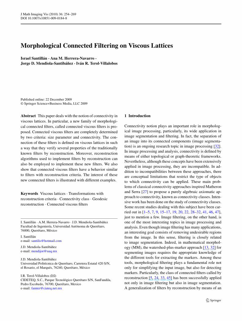
Fig. 1 (a) Original image, (b) morphological closing ϕμ with μ = 7,(c) closing by reconstruction ϕμ with μ = 7, (d) closing with recon-struction criteria γλ,μ with μ = 7 and λ = 3

with λ ≤ μ. The interest of these transformations is illus-trated in Fig. 1. This is the typical problem of connectedoperators called leakage. By using the morphological clos-ing, the word “LETTER” (Fig. 1(a)) is removed and theremaining structures are modified (see Fig. 1(b)). On theother hand, when the closing by reconstruction is applied,the remaining structures kept unchanged but the word hasnot been correctly removed (Fig. 1(c)). Finally, by applyingthe closing with reconstruction criteria ϕλ,μ, one observesin Fig. 1(d) that the remaining structures have not been con-siderably modified and the word has been removed.

3 Connectivity and Filtering on Viscous Lattices

In this section, we will focus on the viscous lattices notionto define a class of connected filters.

3.1 Connectivity and Connected Viscous Filters

First, let us remember an interesting concept that has beenrecently proposed by Serra [30, 31]. In order to characterizethe notion of viscous propagations, Serra replaces the usualspace P(E) by a viscous lattice structure. By establishingthat the family L = {δλ(X), X ∈ P (E)} with λ > 0, isboth the image P (E) under an extensive dilation δλ and un-der the opening δλελ, Serra proposes the viscous lattice asfollows:

258 J Math Imaging Vis (2010) 36: 254–269

Fig. 2 (a) Original image, (b), (c) and (d) morphological openingsusing disks of sizes 10, 20, and 30, respectively

Proposition 1 (Viscous Lattice [31]) The set L is a com-plete lattice regarding the inclusion ordering. In this lattice,the supremum coincides with the set union, whereas the in-fimum ∧ is the opening according to γλ = δλελ of the inter-section.

∧{Xi, i ∈ I } = γλ

(⋂{Xi, i ∈ I }

)

, {Xi, i ∈ I } ∈ L

The universal bounds of L are E and the empty set ∅. L issaid to be the viscous lattice of dilation δλ.

Lλ denotes the image of P (E) under the opening (or thedilation) size λ, and L the image of P (E) under the open-ing or (dilation) for all λ > 0. Figures 2(b)–(d) show threeimages at viscosity 10, 20, 30, respectively. Now, since di-lation δλ is extensive by definition and for every point x,δλ(x) ∈ C , then it preserves the whole class C and the adjointerosion ε treats the connected components independently ofeach other, i.e.

X =⋃

{Xi,Xi ∈ C} ⇒ ελ(X) =⋃

ελ(Xi)

Given that Serra proposes to define connections on P (E)

before the dilation δλB , these connections can be establishedas follows.

Theorem 2 (Serra [31]) Let C be a connection on P (E)

and δλ: P (E) → P (E) be an extensive dilation of adjoint

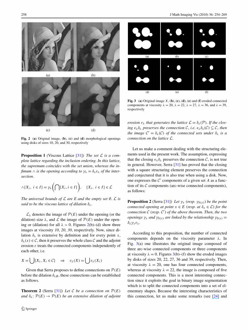
Fig. 3 (a) Original image X, (b), (c), (d), (e) and (f) eroded connectedcomponents at viscosity λ = 20, λ = 22, λ = 27, λ = 36, and λ = 39,respectively

erosion ελ that generates the lattice L = δλ(P ). If the clos-ing ελδλ preserves the connection C , i.e. ελδλ(C) ⊆ C , thenthe image C′ = δλ(C) of the connected sets under δλ is aconnection on the lattice L.

Let us make a comment dealing with the structuring ele-ments used in the present work. The assumption, expressingthat the closing ελδλ preserves the connection C , is not truein general. However, Serra [31] has proved that the closingwith a square structuring element preserves the connectionand conjectured that it is also true when using a disk. Now,one expresses the C′ components of a given set A as a func-tion of its C components (arc-wise connected components),as follows:

Proposition 2 (Serra [31]) Let γx (resp. γδ(x)) be the pointconnected opening at point x ∈ E (resp. at δx ∈ L) for theconnection C (resp. C′) of the above theorem. Then, the twoopenings γx and γδ(x) are linked by the relationship γδ(x) =δλγxελ.

According to this proposition, the number of connectedcomponents depends on the viscosity parameter λ. InFig. 3(a) one illustrates the original image composed ofthree arc-wise connected components or three componentsat viscosity λ = 0. Figures 3(b)–(f) show the eroded imagesby disks of sizes 20, 22, 27, 36 and 39, respectively. Then,at viscosity λ = 20, one has four connected components,whereas at viscosity λ = 22, the image is composed of fiveconnected components. This is a most interesting connec-tion since it exploits the goal in binary image segmentationwhich is to split the connected components into a set of el-ementary shapes. Because the interesting characteristics ofthis connection, let us make some remarks (see [24] and

J Math Imaging Vis (2010) 36: 254–269 259

[33]), concerning traditionally known filters by reconstruc-tion, before introducing a new family of connected filterson viscous lattices. These filters have the fundamental prop-erty of interacting with the image by means of flat zones(which are the largest connected components where the im-age is constant); flat zones are removed or merged. The flatzone notion is an approach for extending connected opera-tors from sets to functions. In the binary case, an operatorψ is said to be connected when for any set A, the symmet-rical difference A � ψ(A) = [A ∩ ψc(A)] ∪ [Ac ∩ ψ(A)]is composed of connected components of A or its comple-ment Ac. Let us show that this is not true when one workswith the connected components of the viscous lattices. First,one assumes that the input image is an element of Lλ, i.e.δλελ(f ) = f .

Since the connectivity of an image depends on the viscos-ity λ, let us classify the connected components in the viscouslattice.

Definition 1 The connected components of Lλ are calledλ-connected components.

Observe that an arc-wise connected component A is aλ-connected component if for all x and y in A, there ex-ists a path p0,p1, . . . , pm with (pk,pk+1) neighbors andλBpk

⊂ A for all k and such that x ∈ λBp0 and y ∈ λBpm .In other words, in the connection of viscous lattices oneneeds to go from one place to another by a continuous pathmade of disks whose centers move along this path. This is amost interesting property of λ-connected components giventhat in our practical problem, the so-called leakage prob-lem, wide flat zones joined by narrow links are forbiddenin this connection. Unlike other interesting connections de-fined by means of a path, for example the partial connectionproposed by Ronse [20] where the union of two overlappingdisks belong to this connection, the viscous lattice connec-tion is better adapted to resolve the leakage problem. Fromthis path definition of λ-connected components it is clearthat a λ2-connected component A of Lλ2 is a λ1-connectedcomponent of Lλ1 with λ1 ≤ λ2, for all connected compo-nents A ∈ Lλ2 , i.e., δλ2ελ2(A) = A ⇒ δλ1ελ1(A) = A. Onthe other hand, in contrast with the arc-wise connectivityin C , where a set X and its complement Xc are composed ofarc-wise connected components, the complement of a set Xin the viscous lattice Lλ is not necessarily composed of λ-connected components. Thus, at viscosity λ and for a givenset X (X = δλελ(X)), the connected components of its com-plement are not λ-connected components (Xc /∈ Lλ). Theonly way for obtaining such a set is to use as input im-age X = γλϕλγλ(X), thus γλ(X) = ϕλ(X) = X. This meansthat X and its complement Xc are composed of λ-connectedcomponents. However, by removing a λ-connected compo-nent of X (for example, using the connected opening intro-duced below γ̃λ,μ), nothing assures that the complement of

the output set is composed of λ-connected components. Thisproblem is a consequence of working in the viscous latticespace, since it does not have the properties of P (E). Forexample, the complement of a viscous set does not neces-sarily belong to the viscous lattice space. Moreover, the vis-cous lattice does not have a lattice-theoretical complemen-tation operation associating to each X a unique X′ such thatX ∧ X′ = ∅ and X ∨ X′ = E. Hence, it is not possible tospeak of connected components for the viscous connectionof the complement of the viscous set. Thus the connectedviscous openings and closings introduced below are definedin terms of connected components of the object and back-ground, respectively. One will see in Sect. 4 that some in-teresting properties fulfilled by filters by reconstruction arealso satisfied by the filters proposed in this section. Now, letus introduce new connected openings and closings into theviscous lattices. Let γo be a trivial opening [5]:

γo(A) =

⎧⎪⎪⎪⎪⎨

⎪⎪⎪⎪⎩

A, if A satisfies an increasing

criterion

∅, if A does not satisfy the

increasing criterion

Similarly, a trivial closing is given by the following rela-tionship:

ϕo(A) =

⎧⎪⎪⎪⎪⎨

⎪⎪⎪⎪⎩

E, if A satisfies an increasing

criterion

A, if A does not satisfy the

increasing criterion

Using these trivial opening and closing, the opening andclosing by reconstruction can be expressed as γ̃ = ∨

x γoγx

and ϕ̃ = ∧x ϕoϕx , respectively. These openings and clos-

ings by reconstruction are established in a general sense -area openings and closings, volume openings and closings,etc. Based on this characterization, the following connectedopening and closing on the viscous lattice can be introduced.

Definition 2 An opening γ̃λ,o (closing ϕ̃λ,o) is a connectedviscous opening (a closing) at viscosity λ if and only if it isconnected in the viscous lattice sense and

γ̃λ,o(X) =∨

x

δλγoγxελ(X) = δλ

∨

x

γoγxελ(X)

= δλγ̃ ελ(X)

ϕ̃λ,o(X) =∧

x

ελϕoϕxδλ(X) = ελ

∧

x

ϕoϕxδλ(X)

= ελϕ̃δλ(X)

(6)

These new filters are also established in a general form;however, the present study is focused on the use of increas-

260 J Math Imaging Vis (2010) 36: 254–269

ing criteria given by the morphological erosion εμ and dila-tion δμ. It is shown later in Sect. 5 that under these increas-ing criteria, connected viscous openings and closings have abehavior similar to openings and closings with reconstruc-tion criteria.

3.2 Geodesic Reconstruction and Filtering

Connected filters are frequently implemented by means ofreconstruction algorithms. Similarly, connected viscous fil-ters on viscous lattices can also be implemented using thesealgorithms. In [47], Wilkinson has shown that even thoughthe great interest of the transformation with reconstructioncriteria ((4) and (5)), the main drawback lies in the com-plexity of computational time. To overcome this inconve-nience a reconstruction process is carried out by floodingthe area to be reconstructed with a viscous liquid as pro-posed by Serra [31]. In the current section, we will focus onthe same reconstruction approach to build connected viscousfilters. It is assumed that the increasing criteria of the trivialopening and closing are established by the morphologicalerosion and dilation, respectively. Thus, the connected vis-cous opening and closing at viscosity λ (with λ ≤ μ) aregiven by:

γ̃λ,μ(f ) = δλR(ελ(f ), εμ−λελ(f ))

= δλR(ελ(f ), εμ(f ))

ϕ̃λ,μ(f ) = ε̃λR∗(δλ(f ), δμ−λδλ(f ))

= ελR∗(δλ(f ), δμ(f ))

(7)

The viscous reconstruction δλR(ελ(f ), εμ(f )) has beenproposed by Serra [31] (see Proposition 2) and clarified byWilkinson [47]. Both transformations, γ̃λ,μ and ϕ̃λ,μ, arenow expressed in terms of reconstruction transformations.The parameter λ determines the viscosity of the transforma-tion and μ the size criterion. Then, to compute γ̃λ,μ, oneselects from the erosion ελ(f ), the regional maxima of sizegreater than or equal to μ − λ, which is equivalent to apply-ing an opening by reconstruction of this size, whereas forcomputing ϕλ,μ, the minima structures of size greater thanor equal to μ−λ are selected from δλ(f ) using a closing byreconstruction. Thus,

γ̃λ,μ(f ) = δλγ̃μ−λελ(f ), ϕ̃λ,μ(f ) = ελϕ̃μ−λδλ(f ) (8)

Now, from (7) and (8), the following inclusion relation-ships can be established:

γμ(f ) = γ̃μ,μ(f ) ≤ γ̃μ−1,μ(f ) ≤ · · · ≤ γ̃1,μ(f )

≤ γ̃0,μ(f ) = γ̃μ(f )

ϕμ(f ) = ϕ̃μ,μ(f ) ≥ ϕ̃μ−1,μ(f ) ≥ · · · ≥ ϕ̃1,μ(f )

≥ ϕ̃0,μ(f ) = ϕ̃μ(f )

(9)

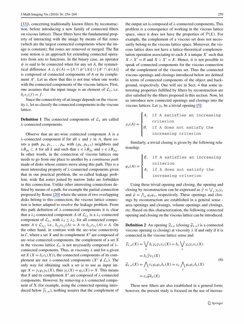
Fig. 4 (a) Original image, (b) and (c) morphological opening γμ withμ, 5 and 15, respectively, (d) and (e) opening by reconstruction γ̃μ

with μ, 5 and 15, respectively, (f) and (g) eroded images εμ of sizes 5and 15, respectively, (h) geodesic reconstruction of reference image (f)from marker image (g), (i) dilated image computed from (h) size 5

For the sake of simplicity let us only prove the order-ing relationships for the opening in the binary case. Ob-serve that from (8), γ̃μ,μ(X) = γμ(X) for λ = μ; whereasfor λ = 0, γ̃0,μ(X) = γ̃μ(X). Now, for a given λ let usshow that γ̃λ+1,μ(X) ⊆ γ̃λ,μ(X) or from (7) one has thatδλδR(ελ+1(X), εμ(X)) ⊆ δλR(ελ(X), εμ(X)). Given theincreasing property of the dilation, one only needs to provethe inclusion δR(ελ+1(X), εμ(X)) ⊆ R(ελ(X), εμ(X)).Since εμ(X) ⊆ ελ+1(X) ⊆ ελ(X), this implies thatR(ελ+1(X), εμ(X)) ⊆ R(ελ(X), εμ(X)). Thus, all con-nected components X

′i ∈ R(ελ+1(X), εμ(X)) are connected

components of ελ+1(X) marked by εμ(X) and there-fore included in the connected components Xi of ελ(X)

marked by εμ(X). Since δελ+1(X) = δεελ(X) ⊆ ελ(X),then δR(ελ+1(X), εμ(X)) ⊆ R(ελ(X), εμ(X)) andγ̃λ+1,μ(X) ⊆ γ̃λ,μ(X).

Figure 4 illustrates the interest of these transformations.To remove the skull from the image in Fig. 4(a), the morpho-logical opening, the opening by reconstruction and the con-nected viscous opening were applied. Figures 4(b) and (c)show the output images computed by the morphologicalopening of size 5 and 15, respectively, whereas Figs. 4(d)and (e) illustrate the output images computed by the open-ing by reconstruction of sizes 5 and 15. The morphologicalopening removes the skull but causes considerable modifi-cations in the remaining structures, while the opening by

J Math Imaging Vis (2010) 36: 254–269 261

reconstruction does not remove the skull. Both parametervalues, 5 and 15, were used to build the connected vis-cous opening. Figures 4(f) and (g) show the eroded imagesof sizes 5 and 15, which were used as the reference andmarker images, respectively, to obtain the image in Fig. 4(h)(R(ε5(f ), ε15(f ))). Finally, this last image was dilated withμ = 5 in order to compute de image in Fig. 4(i). Observe thatthe skull has been removed and the remaining structures arepreserved.

4 Some Properties of Connected Viscous Filters

In Sect. 3, one has discussed the connection derived from theviscous lattice space with the goal of introducing connectedviscous openings and closings. Under these new definitions((7) and (8)), several interesting properties fulfilled by filtersby reconstruction are also satisfied by connected viscous fil-ters. Let us study the effect of these filters on connectedcomponents of the input set. Particularly, the behavior ofthese filters when they form granulometries as establishedby the following definition.

Definition 3 A family of openings {γμi} (respectively clos-

ings {ϕμi}), where μi ∈ {1,2, . . . , n}, is a granulometry (re-

spectively antigranulometry) if for all μi,μj ∈ {1,2, . . . , n}and for all function f ,

μi ≤ μj ⇒ γμi(f ) ≥ γμj

(f )

(resp. ϕμi(f ) ≤ ϕμj

(f ))

Before introducing these properties, let us make some re-marks concerning the λ-connection in the binary case. Here,the study is carried out in a given connectivity λ and the in-put images f or X are considered elements of the viscouslattice Lλ. Thus, the λ parameter remains constant, whereasthe size parameter μ belongs to a family {μk} with k ∈{1,2, . . . , n}. Observe from (7) and (8) that in γ̃μ−λελ(X) =R(ελ(X), εμ(X)), the opening by reconstruction removesarc-wise connected components of ελ(X) smaller than μ−λ

and leaves intact the other connected components. Then, forλ ≤ μ1 ≤ μ2 one has γ̃μ2−λελ(X) = R(ελ(X), εμ2(X)) ⊆γ̃μ1−λελ(X) = R(ελ(X), εμ1(X)); thus, for each connectedcomponent Xi of γ̃μ2−λελ(X), there exists a connected com-ponent X

′j of γ̃μ1−λελ(X) such that Xi = X

′j and δλ(Xi) =

δλ(X′j ). This means that for two elements of a family of

connected viscous openings the following property is estab-lished.

Property 2 Let μ1 and μ2 be two parameters such thatλ ≤ μ1 ≤ μ2. If γδ(x)γ̃λ,μ1 �= ∅ and γδ(x)γ̃λ,μ2(X) �= ∅ thenγδ(x)γ̃λ,μ1(X) = γδ(x)γ̃λ,μ2(X).

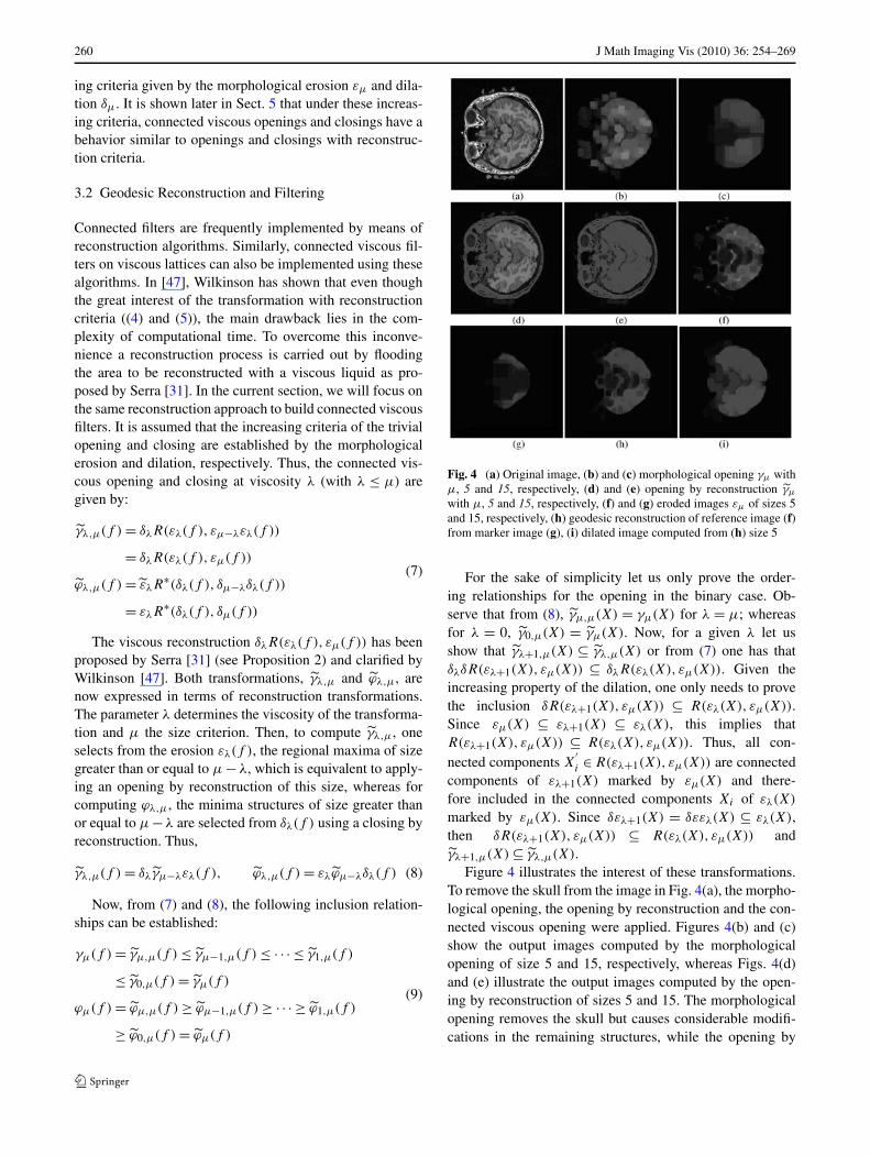
Fig. 5 (a) Input image, (b) eroded image size 20, (c) maxima of imagein (b), (d) contours of λ-maxima, (e) regional maxima of input image,(f), (g) and (h) output images computed by γ̃λ,μ with λ = 20 and μ

values equal to 25, 28, and 32, respectively, (i), (j) and (k) output im-ages computed by γ̃μk−λελ(f ) with λ = 20 and μ values equal to 25,28, and 32, respectively

Remember that γδ(x) = δλγxελ and each connected com-ponent in ελ(γ̃λ,μ2(X)) also exists in ελ(γ̃λ,μ1(X)). Thus,as the parameter k varies, the λ-connected components inγ̃λ,μk

(X) remain identical or vanish. This property can beextended to the function case by working with the maxima(also the minima) notion and the flat zone concept. In or-der to be congruent with the λ-connected components, onecalls these features λ-flat zones and λ-maxima. In Fig. 5the difference between λ-maxima and regional maxima isillustrated. Figures 5(b) and (c) show the eroded image size20, computed from 5(a) and its maxima, respectively. Theeroded image contains nine maxima, hence the original im-age in Fig. 5(a) has nine λ-maxima (at viscosity λ = 20),as illustrated in Fig. 5(d). Only their contours are shownto better illustrate λ-maxima. Compare these λ-maxima,with the regional maxima shown in Fig. 5(e). On the otherhand, Figs. 5(f), (g) and (h) illustrate the output imagescomputed by γ̃λ,μ with λ = 20 and μ values 25, 28 and32, respectively. The opening by reconstruction in the term

262 J Math Imaging Vis (2010) 36: 254–269

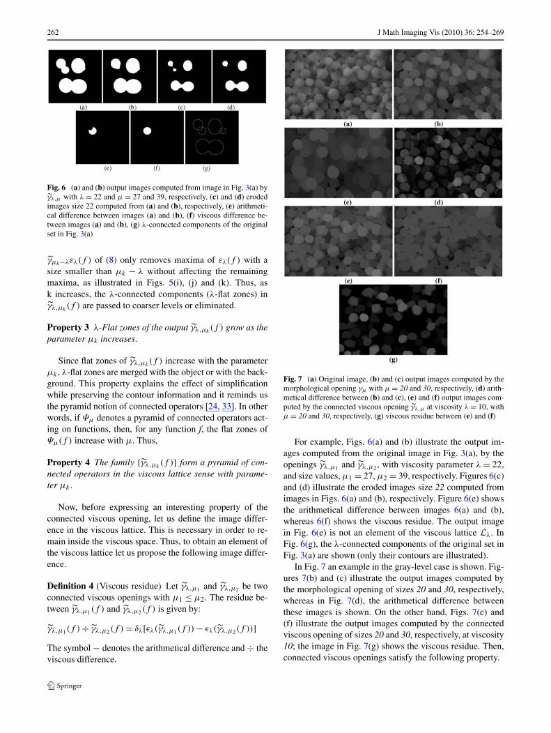
Fig. 6 (a) and (b) output images computed from image in Fig. 3(a) byγ̃λ,μ with λ = 22 and μ = 27 and 39, respectively, (c) and (d) erodedimages size 22 computed from (a) and (b), respectively, (e) arithmeti-cal difference between images (a) and (b), (f) viscous difference be-tween images (a) and (b), (g) λ-connected components of the originalset in Fig. 3(a)

γ̃μk−λελ(f ) of (8) only removes maxima of ελ(f ) with asize smaller than μk − λ without affecting the remainingmaxima, as illustrated in Figs. 5(i), (j) and (k). Thus, ask increases, the λ-connected components (λ-flat zones) inγ̃λ,μk

(f ) are passed to coarser levels or eliminated.

Property 3 λ-Flat zones of the output γ̃λ,μk(f ) grow as the

parameter μk increases.

Since flat zones of γ̃λ,μk(f ) increase with the parameter

μk , λ-flat zones are merged with the object or with the back-ground. This property explains the effect of simplificationwhile preserving the contour information and it reminds usthe pyramid notion of connected operators [24, 33]. In otherwords, if Ψμ denotes a pyramid of connected operators act-ing on functions, then, for any function f, the flat zones ofΨμ(f ) increase with μ. Thus,

Property 4 The family {γ̃λ,μk(f )} form a pyramid of con-

nected operators in the viscous lattice sense with parame-ter μk .

Now, before expressing an interesting property of theconnected viscous opening, let us define the image differ-ence in the viscous lattice. This is necessary in order to re-main inside the viscous space. Thus, to obtain an element ofthe viscous lattice let us propose the following image differ-ence.

Definition 4 (Viscous residue) Let γ̃λ,μ1 and γ̃λ,μ2 be twoconnected viscous openings with μ1 ≤ μ2. The residue be-tween γ̃λ,μ1(f ) and γ̃λ,μ2(f ) is given by:

γ̃λ,μ1(f ) ÷ γ̃λ,μ2(f ) = δλ[ελ(γ̃λ,μ1(f )) − ελ(γ̃λ,μ2(f ))]The symbol − denotes the arithmetical difference and ÷ theviscous difference.

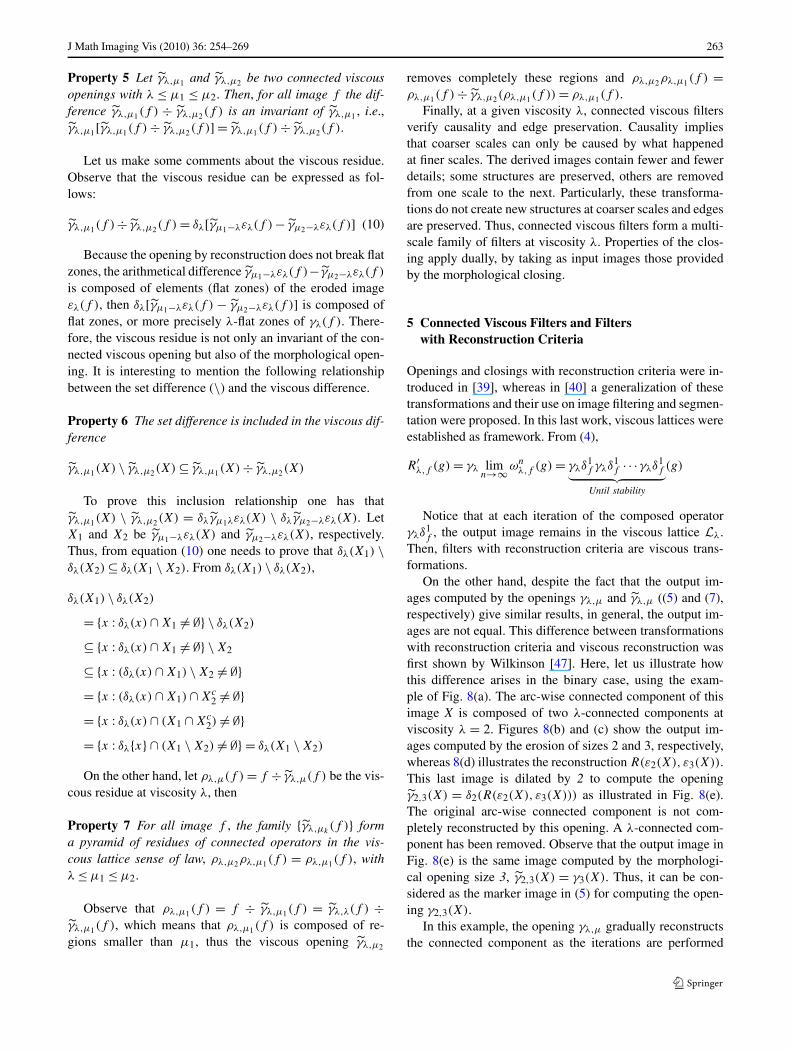
Fig. 7 (a) Original image, (b) and (c) output images computed by themorphological opening γμ with μ = 20 and 30, respectively, (d) arith-metical difference between (b) and (c), (e) and (f) output images com-puted by the connected viscous opening γ̃λ,μ at viscosity λ = 10, withμ = 20 and 30, respectively, (g) viscous residue between (e) and (f)

For example, Figs. 6(a) and (b) illustrate the output im-ages computed from the original image in Fig. 3(a), by theopenings γ̃λ,μ1 and γ̃λ,μ2 , with viscosity parameter λ = 22,and size values, μ1 = 27, μ2 = 39, respectively. Figures 6(c)and (d) illustrate the eroded images size 22 computed fromimages in Figs. 6(a) and (b), respectively. Figure 6(e) showsthe arithmetical difference between images 6(a) and (b),whereas 6(f) shows the viscous residue. The output imagein Fig. 6(e) is not an element of the viscous lattice Lλ. InFig. 6(g), the λ-connected components of the original set inFig. 3(a) are shown (only their contours are illustrated).

In Fig. 7 an example in the gray-level case is shown. Fig-ures 7(b) and (c) illustrate the output images computed bythe morphological opening of sizes 20 and 30, respectively,whereas in Fig. 7(d), the arithmetical difference betweenthese images is shown. On the other hand, Figs. 7(e) and(f) illustrate the output images computed by the connectedviscous opening of sizes 20 and 30, respectively, at viscosity10; the image in Fig. 7(g) shows the viscous residue. Then,connected viscous openings satisfy the following property.

J Math Imaging Vis (2010) 36: 254–269 263

Property 5 Let γ̃λ,μ1 and γ̃λ,μ2 be two connected viscousopenings with λ ≤ μ1 ≤ μ2. Then, for all image f the dif-ference γ̃λ,μ1(f ) ÷ γ̃λ,μ2(f ) is an invariant of γ̃λ,μ1 , i.e.,γ̃λ,μ1[γ̃λ,μ1(f ) ÷ γ̃λ,μ2(f )] = γ̃λ,μ1(f ) ÷ γ̃λ,μ2(f ).

Let us make some comments about the viscous residue.Observe that the viscous residue can be expressed as fol-lows:

γ̃λ,μ1(f ) ÷ γ̃λ,μ2(f ) = δλ[γ̃μ1−λελ(f ) − γ̃μ2−λελ(f )] (10)

Because the opening by reconstruction does not break flatzones, the arithmetical difference γ̃μ1−λελ(f )− γ̃μ2−λελ(f )

is composed of elements (flat zones) of the eroded imageελ(f ), then δλ[γ̃μ1−λελ(f ) − γ̃μ2−λελ(f )] is composed offlat zones, or more precisely λ-flat zones of γλ(f ). There-fore, the viscous residue is not only an invariant of the con-nected viscous opening but also of the morphological open-ing. It is interesting to mention the following relationshipbetween the set difference (\) and the viscous difference.

Property 6 The set difference is included in the viscous dif-ference

γ̃λ,μ1(X) \ γ̃λ,μ2(X) ⊆ γ̃λ,μ1(X) ÷ γ̃λ,μ2(X)

To prove this inclusion relationship one has thatγ̃λ,μ1(X) \ γ̃λ,μ2(X) = δλγ̃μ1λελ(X) \ δλγ̃μ2−λελ(X). LetX1 and X2 be γ̃μ1−λελ(X) and γ̃μ2−λελ(X), respectively.Thus, from equation (10) one needs to prove that δλ(X1) \δλ(X2) ⊆ δλ(X1 \ X2). From δλ(X1) \ δλ(X2),

δλ(X1) \ δλ(X2)

= {x : δλ(x) ∩ X1 �= ∅} \ δλ(X2)

⊆ {x : δλ(x) ∩ X1 �= ∅} \ X2

⊆ {x : (δλ(x) ∩ X1) \ X2 �= ∅}= {x : (δλ(x) ∩ X1) ∩ Xc

2 �= ∅}= {x : δλ(x) ∩ (X1 ∩ Xc

2) �= ∅}= {x : δλ{x} ∩ (X1 \ X2) �= ∅} = δλ(X1 \ X2)

On the other hand, let ρλ,μ(f ) = f ÷ γ̃λ,μ(f ) be the vis-cous residue at viscosity λ, then

Property 7 For all image f , the family {γ̃λ,μk(f )} form

a pyramid of residues of connected operators in the vis-cous lattice sense of law, ρλ,μ2ρλ,μ1(f ) = ρλ,μ1(f ), withλ ≤ μ1 ≤ μ2.

Observe that ρλ,μ1(f ) = f ÷ γ̃λ,μ1(f ) = γ̃λ,λ(f ) ÷γ̃λ,μ1(f ), which means that ρλ,μ1(f ) is composed of re-gions smaller than μ1, thus the viscous opening γ̃λ,μ2

removes completely these regions and ρλ,μ2ρλ,μ1(f ) =ρλ,μ1(f ) ÷ γ̃λ,μ2(ρλ,μ1(f )) = ρλ,μ1(f ).

Finally, at a given viscosity λ, connected viscous filtersverify causality and edge preservation. Causality impliesthat coarser scales can only be caused by what happenedat finer scales. The derived images contain fewer and fewerdetails; some structures are preserved, others are removedfrom one scale to the next. Particularly, these transforma-tions do not create new structures at coarser scales and edgesare preserved. Thus, connected viscous filters form a multi-scale family of filters at viscosity λ. Properties of the clos-ing apply dually, by taking as input images those providedby the morphological closing.

5 Connected Viscous Filters and Filterswith Reconstruction Criteria

Openings and closings with reconstruction criteria were in-troduced in [39], whereas in [40] a generalization of thesetransformations and their use on image filtering and segmen-tation were proposed. In this last work, viscous lattices wereestablished as framework. From (4),

R′λ,f (g) = γλ lim

n→∞ωnλ,f (g) = γλδ

1f γλδ

1f · · ·γλδ

1f

︸ ︷︷ ︸Until stability

(g)

Notice that at each iteration of the composed operatorγλδ

1f , the output image remains in the viscous lattice Lλ.

Then, filters with reconstruction criteria are viscous trans-formations.

On the other hand, despite the fact that the output im-ages computed by the openings γλ,μ and γ̃λ,μ ((5) and (7),respectively) give similar results, in general, the output im-ages are not equal. This difference between transformationswith reconstruction criteria and viscous reconstruction wasfirst shown by Wilkinson [47]. Here, let us illustrate howthis difference arises in the binary case, using the exam-ple of Fig. 8(a). The arc-wise connected component of thisimage X is composed of two λ-connected components atviscosity λ = 2. Figures 8(b) and (c) show the output im-ages computed by the erosion of sizes 2 and 3, respectively,whereas 8(d) illustrates the reconstruction R(ε2(X), ε3(X)).This last image is dilated by 2 to compute the openingγ̃2,3(X) = δ2(R(ε2(X), ε3(X))) as illustrated in Fig. 8(e).The original arc-wise connected component is not com-pletely reconstructed by this opening. A λ-connected com-ponent has been removed. Observe that the output image inFig. 8(e) is the same image computed by the morphologi-cal opening size 3, γ̃2,3(X) = γ3(X). Thus, it can be con-sidered as the marker image in (5) for computing the open-ing γ2,3(X).

In this example, the opening γλ,μ gradually reconstructsthe connected component as the iterations are performed

264 J Math Imaging Vis (2010) 36: 254–269

Fig. 8 (a) Original image X, (b) erosion size 2 (ε2(X)), (c) ero-sion size 3 (ε3(X)), (d) reconstruction R(ε2(X), ε3(X)), (e) dila-tion size 2 of image in (d) γ̃2,3(X) = δ2[R(ε2(X), ε3(X))], (f) out-put image, first iteration, γλδ

1X(γ̃2,3(X)), (g) output image, second

iteration, γλδ1Xγλδ

1X(γ̃2,3(X)) = (γλδ

1X)2(γ̃2,3(X)), (h) output image,

third iteration, (γλδ1X)3(γ̃2,3(X)), (i) output image, until stability,

(γλδ1X)n(γ̃2,3(X)), (j) union of overlapping disks

(Figs. 8(f)–(i)): first iteration γλδ1X(γ̃2,3(X)) (see Fig. 8(f));

second iteration γλδ1Xγλδ

1X(γ̃2,3(X)) = (γλδ

1X)2(γ̃2,3(X))

(Fig. 8(g)); third iteration (γλδ1X)3 (γ̃2,3(X)) (Fig. 8(h)), and

until stability (γλδ1X)n(γ̃2,3(X)) (Fig. 8(i)). Thus, the open-

ing γλ,μ reconstructs more than the opening γ̃λ,μ, and theoutput image computed by γλ,μ is not composed of one λ-connected component, as is the case in γ̃λ,μ, but of bothoriginal λ-connected components. This means, that this re-sult is not congruent with the size criterion given by μ = 3,since a λ-connected component of size 2 has been preserved.This problem is directly linked to a comment made in Sect. 3with regard to the connection on viscous lattices where oneneeds to go from a point x to a point y by a continuous pathmade of disks whose centers move along this path. This isnot true for the transformations with reconstruction crite-ria as illustrated in Fig. 8(j) where one observes that it isnot possible to go from x to y by means of a continuouspath. Therefore, a connection on transformations with re-construction criteria must be introduced using a partial con-nection where the union of two overlapping disks belongs tothis connection as proposed by Ronse [20]. Figure 8(j) onlyshows the squares for the extreme points of the path.

A real example to compare the output images of bothopenings is illustrated in Fig. 9. Figures 9(b) and (c) show

Fig. 9 (a) Original image, (b) and (c) output images computed byγλ,μ and γ̃λ,μ, respectively, (d) the regions with different gray levelsbetween images (b) and (c) are seen as white points

the output images computed by γλ,μ and γ̃λ,μ from the orig-inal image in Fig. 9(a). Visually, both images are the same;however, in Fig. 9(d) the white points show the regions withdifferent gray level values. These regions correspond to sim-ilar configurations as the ones illustrated in Fig. 8.

6 Alternating Sequential Filters

Even though both families, {γ̃λ,μi} and {ϕ̃λ,μi

}, have simi-lar properties than {γ̃μi

} and {ϕ̃μi}, little can be said about

the properties of the families {γ̃λ,μiϕ̃λ,μi

} and {ϕ̃λ,μiγ̃λ,μi

}when compared with filters by reconstruction. For example,the equality (see [5]) γ̃μi

ϕ̃μiγ̃μi

= ϕ̃μiγ̃μi

fulfilled by filtersby reconstructions is not satisfied by connected viscous fil-ters, γ̃λ,μi

ϕ̃λ,μiγ̃λ,μi

�= ϕ̃λ,μiγ̃λ,μi

.However, from a practical point of view, these filters have

interesting characteristics as it is shown in this section. It iswell-known that when structures (dark and bright) that areto be removed from the image have a wide range of scales,the use of a sequence of an opening (closing) followed by aclosing (opening) does not lead to acceptable results. A solu-tion to this problem is the use of alternating sequential filters(ASFs) (see [6, 26, 34, 35, 37]). Serra defines and character-izes four operators mμ(f ) = γμϕμ(f ), nμ(f ) = ϕμγμ(f ),rμ(f ) = ϕμγμϕμ(f ), sμ(f ) = γμϕμγμ(f ), where the sizeof the structuring element μ is indexed over a size distri-bution with 1 ≤ μ ≤ ν. Let us take two of these operators

J Math Imaging Vis (2010) 36: 254–269 265

Fig. 10 (a) Original image, (b) ASF using connected viscous open-ings and closings, (c) ASF using openings and closings by reconstruc-tion

defined as follows:

mλ,μ(f ) = γ̃λ,μϕ̃λ,μ(f ), nλ,μ(f ) = ϕ̃λ,μγ̃λ,μ(f ) (11)

The following inequalities have been introduced andproved in [26, 34], for morphological openings and closings.Here, these inequalities are expressed in terms of connectedviscous openings and closings. For a fixed parameter μ andparameters λ1, λ2 with λ1 ≤ λ2 ≤ μ, one has that:

mλ2,μmλ1,μ(f ) ≤ mλ2,μ(f ) ≤ mλ1,μmλ2,μ(f )

nλ1,μnλ2,μ(f ) ≤ nλ2,μ(f ) ≤ nλ2,μnλ1,μ(f )

Let us prove the inequality mλ2,μmλ1,μ(f ) ≤ mλ2,μ(f ) ≤mλ1,μmλ2,μ(f ) (see [26, 34]). Given that γ̃λ,μ is anti-extensive one has γ̃λ1,μϕ̃λ1,μ(f ) ≤ ϕ̃λ1,μ(f ) and from (9)ϕ̃λ1,μ(f ) ≤ ϕ̃λ2,μ(f ) hence γ̃λ1,μϕ̃λ1,μ(f ) ≤ ϕ̃λ2,μ(f ). ϕ̃λ,μ

being increasing and idempotent ϕ̃λ2,μγ̃λ1,μϕ̃λ1,μ(f ) ≤ϕ̃λ2,μϕ̃λ2,μ(f ) = ϕ̃λ2,μ(f ). Now, γ̃λ,μ is also increasing,hence γ̃λ2,μϕ̃λ2,μγ̃λ1,μϕ̃λ1,μ(f ) ≤ γ̃λ2,μϕ̃λ2,μ(f ), i.e.mλ2,μmλ1,μ(f ) ≤ mλ2,μ(f ). Similarly, f ≤ ϕ̃λ,μ(f ) andγ̃λ,μ is increasing, hence γ̃λ1,μ(f ) ≤ γ̃λ1,μϕ̃λ1,μ(f ). Thus,since γ̃λ2,μ(f ) ≤ γ̃λ1,μ(f ) (see (9)), then γ̃λ2,μ(f ) ≤γ̃λ1,μϕ̃λ1,μ(f ). Now, since γ̃λ,μ is idempotent, γ̃λ2,μγ̃λ2,μ(f )

= γ̃λ2,μ(f ) ≤ γ̃λ1,μϕ̃λ1,μγ̃λ2,μ(f ) and then γ̃λ2,μϕ̃λ2,μ(f ) ≤γ̃λ1,μϕ̃λ1,μγ̃λ2,μϕ̃λ2,μ(f ), i.e. mλ2,μ(f ) ≤ mλ1,μmλ2,μ(f ).

A similar proof can be used for nλ1,μnλ2,μ(f ) ≤ nλ2,μ(f )

≤ nλ2,μnλ1,μ(f ).Since the connected viscous opening and closing take

two parameters, let us use the μ parameter as the size ofthe structures of the image to be preserved and the λ pa-rameter as the size of those structures linked to the struc-tures to be preserved. While the size parameter μ detectsthe main structures, the λ parameter permits the smoothingof these structures. Then, from (11) and for a family {λi}

Fig. 11 (a) Original image, (b) alternating filter γ̃μϕ̃μ(f ) withμ = 25, (c) ASF γ4ϕ4γ3ϕ3γ2ϕ2γ1ϕ1(f ), (d) alternating filterγ̃λ,μϕ̃λ,μ(f ) with μ = 25 and λ = 4, (e) ASF γ̃4,μϕ̃4,μγ̃3,μϕ̃3,μ

γ̃2,μϕ̃2,μγ̃1,μϕ̃1,μ(f ) with μ = 25, (f) ASF γ̃4,μϕ̃4,μγ̃2,μϕ̃2,μ(f ) withμ = 25

with λj < λk if j < k, the following alternating sequentialfilters are defined:

Mλn,μ(f ) = mλn,μ . . .mλ2,μmλ1,μ(f )

Nλn,μ(f ) = nλn,μ . . . nλ2,μnλ1,μ(f )(12)

with the condition λn ≤ μ. Figures 10(b) and (c) show theoutput images computed by an ASF using connected vis-cous filters and an ASF by reconstruction. Another exam-ple illustrating the differences between two kinds of ASF isshown in Fig. 11. The image in Fig. 11(b) shows the out-put image computed from the original image in Fig. 11(a)by the alternate filter using an opening and closing by re-construction γ̃μϕ̃μ(f ) with μ = 25, while the image inFig. 11(c) was computed by ASF γ4ϕ4γ3ϕ3γ2ϕ2γ1ϕ1(f ).Observe that the alternating filter, using reconstruction fil-ters, enables the extraction of the main structure of the im-age by removing all regions not connected to this struc-ture; while the ASF, using morphological openings and clos-ings, allows the removal of some structures linked to themain region (the cameraman). The idea of using connectedviscous openings and closings consists in taking into ac-count both behaviors. Then, let us apply a sequence ofconnected viscous openings and closings. The images inFigs. 11(d) to (f) illustrate the use of ASFs using connectedviscous openings and closings. The image in Fig. 11(d)was computed by using the filter γ̃λ,μϕ̃λ,μ(f ) with μ =25 and λ = 4, whereas in Fig. 11(e) the result of usingASF γ̃4,μϕ̃4,μγ̃3,μϕ̃3,μγ̃2,μϕ̃2,μγ̃1,μϕ̃1,μ(f ) with μ = 25 isshown. Finally, the image in Fig. 11(f) was computed withASF γ̃4,μϕ̃4,μγ̃2,μϕ̃2,μ(f ) and μ = 25.

On the other hand, in Fig. 12 the above-described prob-lem of removing the skull is illustrated. Figures 12(b) and (c)

266 J Math Imaging Vis (2010) 36: 254–269

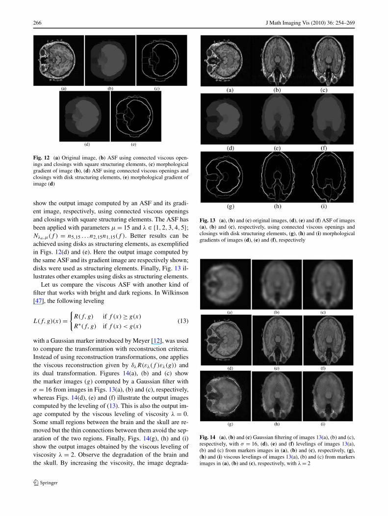
Fig. 12 (a) Original image, (b) ASF using connected viscous open-ings and closings with square structuring elements, (c) morphologicalgradient of image (b), (d) ASF using connected viscous openings andclosings with disk structuring elements, (e) morphological gradient ofimage (d)

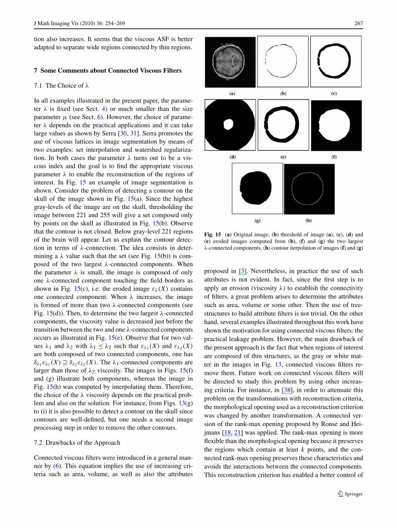
show the output image computed by an ASF and its gradi-ent image, respectively, using connected viscous openingsand closings with square structuring elements. The ASF hasbeen applied with parameters μ = 15 and λ ∈ {1,2,3,4,5};Nλn,μ(f ) = n5,15 . . . n2,15n1,15(f ). Better results can beachieved using disks as structuring elements, as exemplifiedin Figs. 12(d) and (e). Here the output image computed bythe same ASF and its gradient image are respectively shown;disks were used as structuring elements. Finally, Fig. 13 il-lustrates other examples using disks as structuring elements.

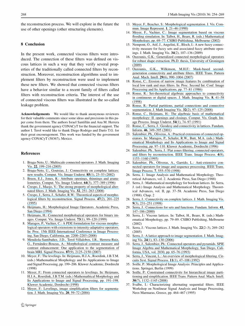
Let us compare the viscous ASF with another kind offilter that works with bright and dark regions. In Wilkinson[47], the following leveling

L(f,g)(x) ={

R(f,g) if f (x) ≥ g(x)

R∗(f, g) if f (x) < g(x)(13)

with a Gaussian marker introduced by Meyer [12], was usedto compare the transformation with reconstruction criteria.Instead of using reconstruction transformations, one appliesthe viscous reconstruction given by δλR(ελ(f )ελ(g)) andits dual transformation. Figures 14(a), (b) and (c) showthe marker images (g) computed by a Gaussian filter withσ = 16 from images in Figs. 13(a), (b) and (c), respectively,whereas Figs. 14(d), (e) and (f) illustrate the output imagescomputed by the leveling of (13). This is also the output im-age computed by the viscous leveling of viscosity λ = 0.Some small regions between the brain and the skull are re-moved but the thin connections between them avoid the sep-aration of the two regions. Finally, Figs. 14(g), (h) and (i)show the output images obtained by the viscous leveling ofviscosity λ = 2. Observe the degradation of the brain andthe skull. By increasing the viscosity, the image degrada-

Fig. 13 (a), (b) and (c) original images, (d), (e) and (f) ASF of images(a), (b) and (c), respectively, using connected viscous openings andclosings with disk structuring elements, (g), (h) and (i) morphologicalgradients of images (d), (e) and (f), respectively

Fig. 14 (a), (b) and (c) Gaussian filtering of images 13(a), (b) and (c),respectively, with σ = 16, (d), (e) and (f) levelings of images 13(a),(b) and (c) from markers images in (a), (b) and (c), respectively, (g),(h) and (i) viscous levelings of images 13(a), (b) and (c) from markersimages in (a), (b) and (c), respectively, with λ = 2

J Math Imaging Vis (2010) 36: 254–269 267

tion also increases. It seems that the viscous ASF is betteradapted to separate wide regions connected by thin regions.

7 Some Comments about Connected Viscous Filters

7.1 The Choice of λ

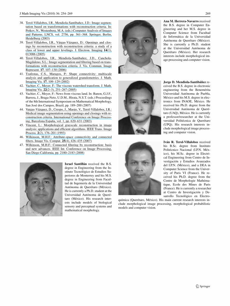
In all examples illustrated in the present paper, the parame-ter λ is fixed (see Sect. 4) or much smaller than the sizeparameter μ (see Sect. 6). However, the choice of parame-ter λ depends on the practical applications and it can takelarge values as shown by Serra [30, 31]. Serra promotes theuse of viscous lattices in image segmentation by means oftwo examples: set interpolation and watershed regulariza-tion. In both cases the parameter λ turns out to be a vis-cous index and the goal is to find the appropriate viscousparameter λ to enable the reconstruction of the regions ofinterest. In Fig. 15 an example of image segmentation isshown. Consider the problem of detecting a contour on theskull of the image shown in Fig. 15(a). Since the highestgray-levels of the image are on the skull, thresholding theimage between 221 and 255 will give a set composed onlyby points on the skull as illustrated in Fig. 15(b). Observethat the contour is not closed. Below gray-level 221 regionsof the brain will appear. Let us explain the contour detec-tion in terms of λ-connection. The idea consists in deter-mining a λ value such that the set (see Fig. 15(b)) is com-posed of the two largest λ-connected components. Whenthe parameter λ is small, the image is composed of onlyone λ-connected component touching the field borders asshown in Fig. 15(c), i.e. the eroded image ελ(X) containsone connected component. When λ increases, the imageis formed of more than two λ-connected components (seeFig. 15(d)). Then, to determine the two largest λ-connectedcomponents, the viscosity value is decreased just before thetransition between the two and one λ-connected componentsoccurs as illustrated in Fig. 15(e). Observe that for two val-ues λ1 and λ2 with λ1 ≤ λ2 such that ελ1(X) and ελ2(X)

are both composed of two connected components, one hasδλ1ελ1(X) ⊇ δλ2ελ2(X). The λ1-connected components arelarger than those of λ2 viscosity. The images in Figs. 15(f)and (g) illustrate both components, whereas the image inFig. 15(h) was computed by interpolating them. Therefore,the choice of the λ viscosity depends on the practical prob-lem and also on the solution. For instance, from Figs. 13(g)to (i) it is also possible to detect a contour on the skull sincecontours are well-defined, but one needs a second imageprocessing step in order to remove the other contours.

7.2 Drawbacks of the Approach

Connected viscous filters were introduced in a general man-ner by (6). This equation implies the use of increasing cri-teria such as area, volume, as well as also the attributes

Fig. 15 (a) Original image, (b) threshold of image (a), (c), (d) and(e) eroded images computed from (b), (f) and (g) the two largestλ-connected components, (h) contour iterpolation of images (f) and (g)

proposed in [3]. Nevertheless, in practice the use of suchattributes is not evident. In fact, since the first step is toapply an erosion (viscosity λ) to establish the connectivityof filters, a great problem arises to determine the attributessuch as area, volume or some other. Then the use of tree-structures to build attribute filters is not trivial. On the otherhand, several examples illustrated throughout this work haveshown the motivation for using connected viscous filters: thepractical leakage problem. However, the main drawback ofthe present approach is the fact that when regions of interestare composed of thin structures, as the gray or white mat-ter in the images in Fig. 13, connected viscous filters re-move them. Future work on connected viscous filters willbe directed to study this problem by using other increas-ing criteria. For instance, in [38], in order to attenuate thisproblem on the transformations with reconstruction criteria,the morphological opening used as a reconstruction criterionwas changed by another transformation. A connected ver-sion of the rank-max opening proposed by Ronse and Hei-jmans [18, 21] was applied. The rank-max opening is moreflexible than the morphological opening because it preservesthe regions which contain at least k points, and the con-nected rank-max opening preserves these characteristics andavoids the interactions between the connected components.This reconstruction criterion has enabled a better control of

268 J Math Imaging Vis (2010) 36: 254–269

the reconstruction process. We will explore in the future theuse of other openings (other structuring elements).

8 Conclusion

In the present work, connected viscous filters were intro-duced. The connection of these filters was defined on vis-cous lattices in such a way that they verify several prop-erties of the traditionally called connected filters by recon-struction. Moreover, reconstruction algorithms used to im-plement filters by reconstruction were used to implementthese new filters. We showed that connected viscous filtershave a behavior similar to a recent family of filters calledfilters with reconstruction criteria. The interest of the useof connected viscous filters was illustrated in the so-calledleakage problem.

Acknowledgements We would like to thank anonymous reviewersfor their valuable comments since some ideas and precisions in this pa-per come from them. The authors Israel Santillán and Ana M. Herrerathank the government agency CONACyT for the financial support. Theauthor I. Terol would like to thank Diego Rodrigo and Darío T.G. fortheir great encouragement. This work was funded by the governmentagency CONACyT (58367), Mexico.

References

1. Braga-Neto, U.: Multiscale connected operators. J. Math. ImagingVis. 22, 199–216 (2005)

2. Braga-Neto, U., Goutsias, J.: Connectivity on complete lattices:new results. Comput. Vis. Image Underst. 85(1), 23–53 (2002)

3. Breen, E.J., Jones, R.: Attribute openings, thinnings and granu-lometries. Comput. Vis. Image Underst. 64(3), 377–389 (1996)

4. Crespo, J., Maojo, V.: The strong property of morphological alter-nated filters. J. Math. Imaging Vis. 32, 251–263 (2008)

5. Crespo, J., Serra, J., Schafer, R.W.: Theoretical aspects of morpho-logical filters by reconstruction. Signal Process. 47(2), 201–225(1995)

6. Heijmans, H.: Morphological Image Operators. Academic Press,San Diego (1994)

7. Heijmans, H.: Connected morphological operators for binary im-ages. Comput. Vis. Image Underst. 73(1), 99–120 (1999)

8. Maragos, P., Vachier, C.: A PDE formulation for viscous morpho-logical operators with extensions to intensity-adaptative operators.In: Proc. 15th IEEE-International Conference in Image Process-ing, San Diego, California, pp. 2200–2203 (2008)

9. Mendiola-Santibañez, J.D., Terol-Villalobos, I.R., Herrera-Ruiz,G., Fernández-Bouzas, A.: Morphological contrast measure andcontrast enhancement: One application to the segmentation ofbrain MRI. Signal Process. 87(9), 2125–2150 (2007)

10. Meyer, F.: The levelings. In: Heijmans, H.J.A., Roerdink, J.B.T.M.(eds.) Mathemathical Morphology and Its Applications to Imageand Signal Processing, pp. 199–206. Kluwer Academic, Dordrecht(1998)

11. Meyer, F.: From connected operators to levelings. In: Heijmans,H.J.A., Roerdink, J.B.T.M. (eds.) Mathemathical Morphology andIts Applications to Image and Signal Processing, pp. 191–198.Kluwer Academic, Dordrecht (1998)

12. Meyer, F.: Levelings, image simplification filters for segmenta-tion. J. Math. Imaging Vis. 20, 59–72 (2004)

13. Meyer, F., Beucher, S.: Morphological segmentation. J. Vis. Com-mun. Image Represent. 1, 21–46 (1990)

14. Meyer, F., Vachier, C.: Image segmentation based on viscousflooding simulation. In: Talbot, H., Beare, R. (eds.) MathematicalMorphology, pp. 69–77. CSIRO Publishing, Melbourne (2002)

15. Nempont, O., Atif, J., Angelini, E., Bloch, I.: A new fuzzy connec-tivity measure for fuzzy sets and associated fuzzy attribute open-ings. J. Math. Imaging Vis. 34(2), 107–136 (2009)

16. Ouzounis, G.K.: Generalized connected morphological operatorsfor robust shape extraction. Ph.D. thesis, University of Groningen(2009)

17. Ouzounis, G.K., Wilkinson, M.H.F.: Mask-based second-generation connectivity and attribute filters. IEEE Trans. PatternAnal. Mach. Intell. 29(6), 990–1004 (2007)

18. Ronse, C.: Erosion of narrow image features by combination oflocal low rank and max filters. In: Proc. Second Int. Conf. ImageProcessing and Its Applications, pp. 77–81 (1986)

19. Ronse, R.: Set-theoretical algebraic approaches to connectivityin continuous or digital spaces. J. Math. Imaging Vis. 8, 41–58(1998)

20. Ronse, R.: Partial partitions, partial connections and connectivesegmentation. J. Math Imaging Vis. 32(2), 97–125 (2008)

21. Ronse, C., Heijmans, H.: The algebraic basis of mathematicalmorphology: II. openings and closings. Comput. Vis. Graph. Im-age Process. Image Underst. 54(1), 74–97 (1991)

22. Ronse, C., Serra, J.: Geodesy and connectivity in lattices. Fundam.Inform. 46, 349–395 (2001)

23. Salembier, Ph., Oliveras, A.: Practical extensions of connected op-erators. In: Maragos, P., Schafer, R.W., Butt, M.A. (eds.) Math-ematical Morphology and Its Applications to Image and SignalProcessing, pp. 97–110. Kluwer Academic, Dordrecht (1996)

24. Salembier, Ph., Serra, J.: Flat zones filtering, connected operators,and filters by reconstruction. IEEE Trans. Image Process. 4(8),1153–1160 (1995)

25. Salembier, Ph., Oliveras, A., Garrido, L.: Anti-extensive con-nected operators for image and sequence processing. IEEE Trans.Image Process. 7, 555–570 (1998)

26. Serra, J.: Image Analysis and Mathematical Morphology. Theo-retical Advances, vol. 2. Academic Press, San Diego (1988)

27. Serra, J.: Mathematical morphology for boolean lattices. In: Serra,J. (ed.) Image Analysis and Mathematical Morphology. Theoret-ical Advances, vol. II, pp. 37–58. Academic Press, San Diego(1988). Chap. 2

28. Serra, J.: Connectivity on complete lattices. J. Math. Imaging Vis.9(3), 231–251 (1998)

29. Serra, J.: Connections for sets and functions. Fundam. Inform. 41,147–186 (2000)

30. Serra, J.: Viscous lattices. In: Talbot, H., Beare, R. (eds.) Math-ematical Morphology, pp. 79–89. CSIRO Publishing, Melbourne(2002)

31. Serra, J.: Viscous lattices. J. Math. Imaging Vis. 22(2–3), 269–282(2005)

32. Serra, J.: A lattice approach to image segmentation. J. Math. Imag-ing Vis. 24(1), 83–130 (2006)

33. Serra, J., Salembier, Ph.: Connected operators and pyramids. SPIEImage Algebra and Mathematical Morphology, San Diego, Cali-fornia, USA, vol. 2030, pp. 65–76 (1993)

34. Serra, J., Vincent, L.: An overview of morphological filtering. Cir-cuits Syst. Signal Process. 11(1), 47–108 (1992)

35. Soille, P.: Morphological Image Analysis: Principles and Applica-tions. Springer, Berlin (1999)

36. Soille, P.: Constrained connectivity for hierarchical image parti-tioning and simplification. IEEE Trans. Pattern Anal. Mach. Intell.30(7), 1132–1145 (2008)

37. Svalbe, I.: Characterizing alternating sequential filters. IEEEWorkshop on Nonlinear Signal Analysis and Image Processing,Neos Marmaras, Greece, pp. 464–467 (1995)

J Math Imaging Vis (2010) 36: 254–269 269

38. Terol-Villalobos, I.R., Mendiola-Santibañez, J.D.: Image segmen-tation based on transformations with reconstruction criteria. In:Petkov, N., Westenberg, M.A. (eds.) Computer Analysis of Imagesand Patterns. LNCS, vol. 2756, pp. 361–368. Springer, Berlin,Heidelberg (2003)

39. Terol-Villalobos, I.R., Várgas-Vázquez, D.: Openings and clos-ings by reconstruction with reconstruction criteria: a study of aclass of lower and upper levelings. J. Electron. Imaging 14(1),013006 (2005)

40. Terol-Villalobos, I.R., Mendiola-Santibañez, J.D., Canchola-Magdaleno, S.L.: Image segmentation and filtering based on trans-formations with reconstruction criteria. J. Vis. Commun. ImageRepresent. 17, 107–130 (2006)

41. Tzafestas, C.S., Maragos, P.: Shape connectivity: multiscaleanalysis and application to generalized granulometries. J. Math.Imaging Vis. 17, 109–129 (2002)

42. Vachier, C., Meyer, F.: The viscous watershed transform. J. Math.Imaging Vis. 22(2–3), 251–267 (2005)

43. Vachier, C., Meyer, F.: News from viscous land. In: Banon, G.J.F.,Barrera, J., Braga-Neto, U.D.M., Hirata, N.S.T. (eds.) Proceedingsof the 8th International Symposium on Mathematical Morphology,San José dos Campos, Brazil, pp. 189–200 (2007)

44. Vargas-Vázquez, D., Crespo, J., Maojo, V., Terol-Villalobos, I.R.:Medical image segmentation using openings and closings with re-construction criteria. International Conference on Image Process-ing, Barcelona España, vol. 1, pp. 620–631 (2003)

45. Vincent, L.: Morphological grayscale reconstruction in imageanalysis: applications and efficient algorithms. IEEE Trans. ImageProcess. 2(2), 176–201 (1993)

46. Wilkinson, M.H.F.: Attribute-space connectivity and connectedfilters. Image Vis. Comput. 25(4), 426–435 (2007)

47. Wilkinson, M.H.F.: Connected filtering by reconstruction: basisand new advances. IEEE Int. Conference on Image Processing,San Diego California, pp. 2180–2183 (2008)

Israel Santillán received the B.S.degree in Engineering from the In-stituto Tecnológico de Estudios Su-periores de Monterrey and his M.S.degree in Engineering from Facul-tad de Ingeniería de la UniversidadAutónoma de Querétaro (México).He is currently a Ph.D. student at theUniversidad Autónoma de Queré-taro (México). His research inter-ests include models of biologicalsensory and perceptual systems andmathematical morphology.

Ana M. Herrera-Navarro receivedthe B.S. degree in Computer En-gineering and her M.S. degree inComputer Science from Facultadde Informática de la UniversidadAutónoma de Querétaro (México).She is currently a Ph.D. studentat the Universidad Autónoma deQuerétaro (México). Her researchinterests include morphological im-age processing and computer vision.

Jorge D. Mendiola-Santibáñez re-ceived the B.S. degree in electronicengineering from the BeneméritaUniversidad Autónoma de Puebla,México and his M.S. degree in elec-tronics from INAOE, México. Hereceived his Ph.D. degree from theUniversidad Autónoma de Queré-taro (UAQ), México. He is currentlya professor/researcher at the Uni-versidad Politécnica de Querétaro(UPQ). His research interests in-clude morphological image process-ing and computer vision.

Iván R. Terol-Villalobos receivedhis B.Sc. degree from InstitutoPolitécnico Nacional (I.P.N. Méx-ico), his M.Sc. degree in Electri-cal Engineering from Centro de In-vestigación y Estudios Avanzadosdel I.P.N. (México), and a DEA inComputer Science from the Univer-sity of Paris VI (France). He re-ceived his Ph.D. degree from theCentre de Morphologie Mathéma-tique, Ecole des Mines de Paris(France). He is currently a researcherat Centro de Investigación y De-sarrollo Tecnológico en Electro-

química (Querétaro, México). His main current research interests in-clude morphological image processing, morphological probabilisticmodels and computer vision.