More Graphs and Displays 1 Section 2.2. Section 2.2 Objectives Graph quantitative data using stem-and-leaf plots and dot plots Graph qualitative data.

More Graphs and Displays

1

Section 2.2

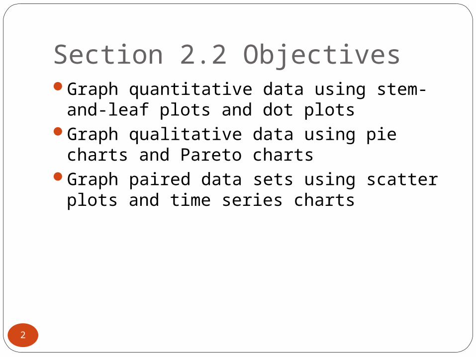
Section 2.2 ObjectivesGraph quantitative data using stem-and-

leaf plots and dot plotsGraph qualitative data using pie charts and

Pareto chartsGraph paired data sets using scatter plots

and time series charts

2

Graphing Quantitative Data Sets

Stem-and-leaf plotEach number is separated into a stem and a

leaf.Similar to a histogram.Still contains original data values.

Data: 21, 25, 25, 26, 27, 28, 30, 36, 36, 45

26

21 5 5 6 7 83 0 6 6

4 5

3

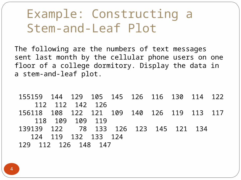
Example: Constructing a Stem-and-Leaf Plot

The following are the numbers of text messages sent last month by the cellular phone users on one floor of a college dormitory. Display the data in a stem-and-leaf plot.

155159 144 129 105 145 126 116 130 114 122 112 112 142 126

156118 108 122 121 109 140 126 119 113 117 118 109 109 119

139139 122 78 133 126 123 145 121 134 124 119 132 133 124

129 112 126 148 147

4

Solution: Constructing a Stem-and-Leaf Plot

• The data entries go from a low of 78 to a high of 159.• Use the rightmost digit as the leaf.

For instance, 78 = 7 | 8 and 159 = 15 | 9

• List the stems, 7 to 15, to the left of a vertical line.• For each data entry, list a leaf to the right of its stem.

155159 144 129 105 145 126 116 130 114 122 112 112 142 126

156118 108 122 121 109 140 126 119 113 117 118 109 109 119

139139 122 78 133 126 123 145 121 134 124 119 132 133 124

129 112 126 148 147

5

Solution: Constructing a Stem-and-Leaf Plot

Include a key to identify the values of the data.

From the display, you can conclude that more than 50% of the cellular phone users sent between 110 and 130 text messages.6

Graphing Quantitative Data Sets

Dot plotEach data entry is plotted, using a point,

above a horizontal axisDots represent an actual data value. Dots

representing the same value are stacked.

Data: 21, 25, 25, 26, 27, 28, 30, 36, 36, 45 26

20 21 22 23 24 25 26 27 28 29 30 31 32 33 34 35 36 37 38 39 40 41 42 43 44 45

7

Example: Constructing a Dot Plot

Use a dot plot organize the text messaging data.

• So that each data entry is included in the dot plot, the horizontal axis should include numbers between 70 and 160.

• To represent a data entry, plot a point above the entry's position on the axis.

• If an entry is repeated, plot another point above the previous point.

155159 144 129 105 145 126 116 130 114 122 112 112 142 126

156118 108 122 121 109 140 126 119 113 117 118 109 109 119

139139 122 78 133 126 123 145 121 134 124 119 132 133 124

129 112 126 148 147

8

Solution: Constructing a Dot Plot

From the dot plot, you can see that most values cluster between 105 and 148 and the value that occurs the most is 126. You can also see that 78 is an unusual data value.

155159 144 129 105 145 126 116 130 114 122 112 112 142 126

156118 108 122 121 109 140 126 119 113 117 118 109 109 119

139139 122 78 133 126 123 145 121 134 124 119 132 133 124

129 112 126 148 147

9

Graphing Qualitative Data Sets

Pie ChartA circle is divided into sectors that represent

categories.The area of each sector is proportional to the

frequency of each category.

10

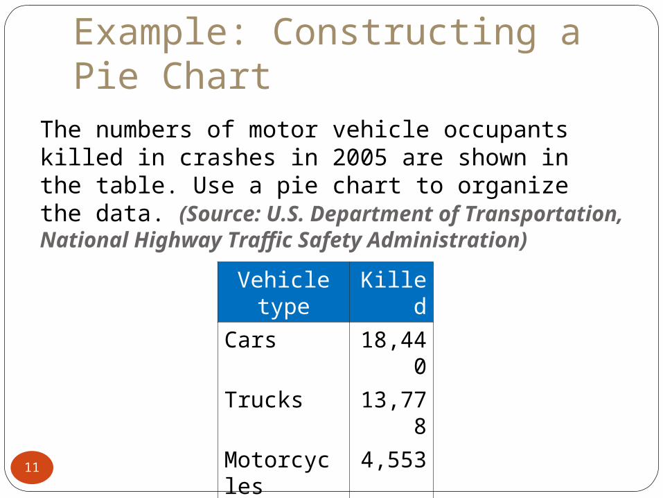
Example: Constructing a Pie Chart

The numbers of motor vehicle occupants killed in crashes in 2005 are shown in the table. Use a pie chart to organize the data. (Source: U.S. Department of Transportation, National Highway Traffic Safety Administration)

Vehicle type

Killed

Cars 18,440

Trucks 13,778

Motorcycles

4,553

Other 823

11

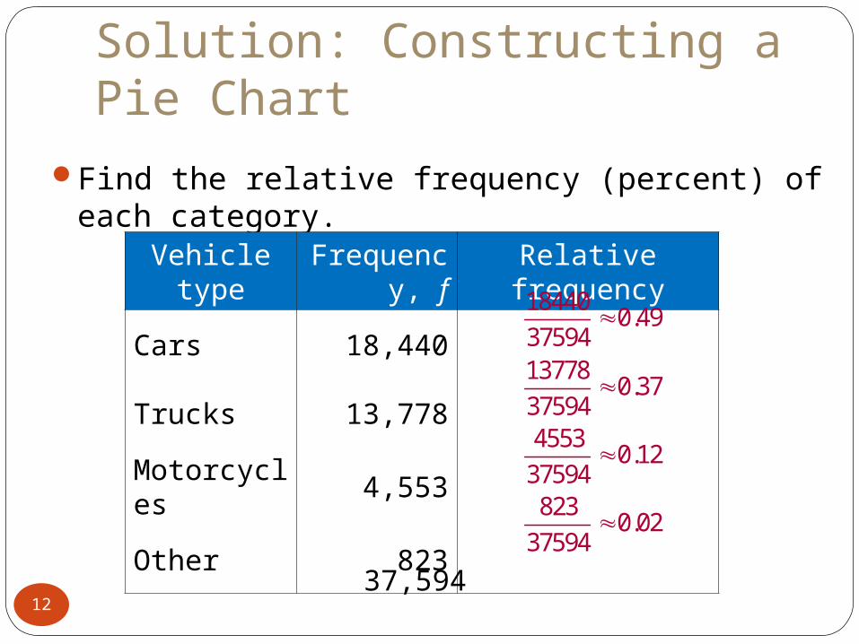
Solution: Constructing a Pie Chart

Find the relative frequency (percent) of each category.

Vehicle type

Frequency, f

Relative frequency

Cars 18,440

Trucks 13,778

Motorcycles

4,553

Other 823

37,594

184400.49

37594

137780.37

37594

45530.12

37594

8230.02

37594

12

Solution: Constructing a Pie Chart

Construct the pie chart using the central angle that corresponds to each category. To find the central angle, multiply 360º

by the category's relative frequency. For example, the central angle for cars is

360(0.49) ≈ 176º

13

Solution: Constructing a Pie Chart

Vehicle type

Frequency, f

Relative frequenc

yCentral angle

Cars 18,440 0.49

Trucks 13,778 0.37

Motorcycles

4,553 0.12

Other 823 0.02

360º(0.49)≈176º

360º(0.37)≈133º

360º(0.12)≈43º

360º(0.02)≈7º

14

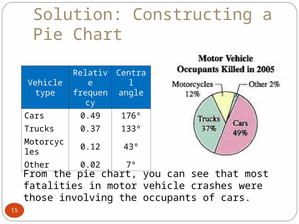
Solution: Constructing a Pie Chart

Vehicle type

Relative frequen

cy

Central angle

Cars 0.49 176º

Trucks 0.37 133º

Motorcycles

0.12 43º

Other 0.02 7º

From the pie chart, you can see that most fatalities in motor vehicle crashes were those involving the occupants of cars.

15

Graphing Qualitative Data Sets

Pareto ChartA vertical bar graph in which the height of each bar

represents frequency or relative frequency.The bars are positioned in order of decreasing

height, with the tallest bar positioned at the left.

Categories

Freq

uen

cy

16

Example: Constructing a Pareto Chart

In a recent year, the retail industry lost $41.0 million in inventory shrinkage. Inventory shrinkage is the loss of inventory through breakage, pilferage, shoplifting, and so on. The causes of the inventory shrinkage are administrative error ($7.8 million), employee theft ($15.6 million), shoplifting ($14.7 million), and vendor fraud ($2.9 million). Use a Pareto chart to organize this data. (Source: National Retail Federation and Center for Retailing Education, University of Florida)

17

Solution: Constructing a Pareto Chart

Cause $ (million)

Admin. error

7.8

Employee theft

15.6

Shoplifting 14.7

Vendor fraud

2.9

From the graph, it is easy to see that the causes of inventory shrinkage that should be addressed first are employee theft and shoplifting.

18

Graphing Paired Data SetsPaired Data SetsEach entry in one data set corresponds to

one entry in a second data set.Graph using a scatter plot.

The ordered pairs are graphed aspoints in a coordinate plane.

Used to show the relationship between two quantitative variables.

x

y

19

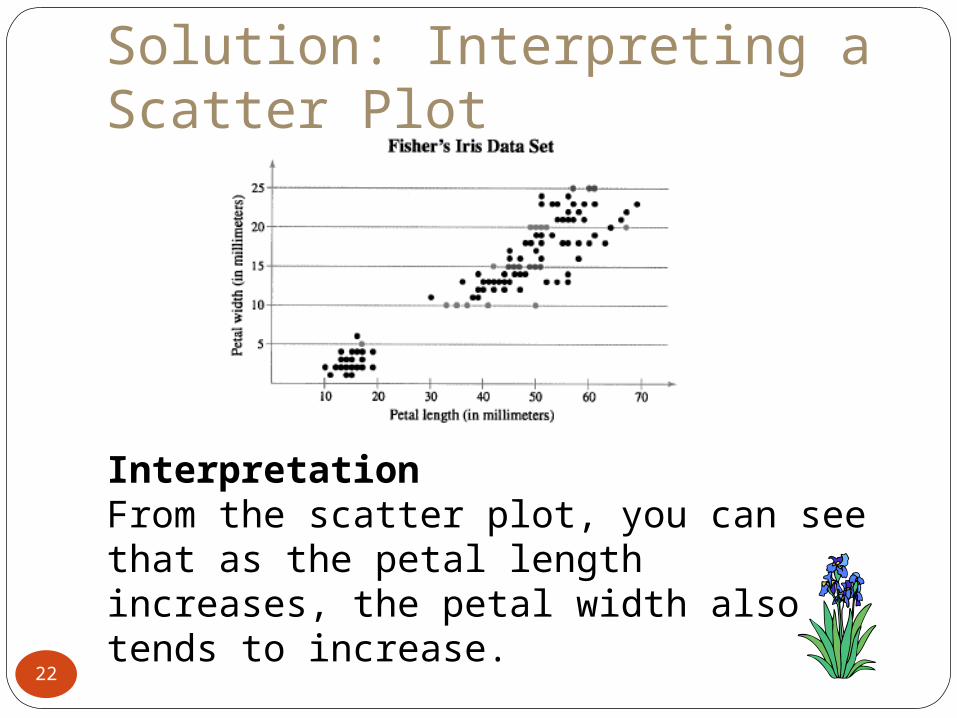
Example: Interpreting a Scatter Plot

The British statistician Ronald Fisher introduced a famous data set called Fisher's Iris data set. This data set describes various physical characteristics, such as petal length and petal width (in millimeters), for three species of iris. The petal lengths form the first data set and the petal widths form the second data set. (Source: Fisher, R. A., 1936)

20

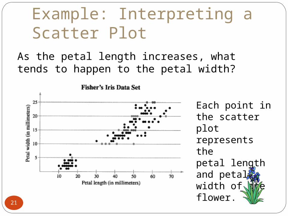
Example: Interpreting a Scatter Plot

As the petal length increases, what tends to happen to the petal width?

Each point in the scatter plot represents thepetal length and petal width of one flower.

21

Solution: Interpreting a Scatter Plot

Interpretation From the scatter plot, you can see that as the petal length increases, the petal width also tends to increase.

22

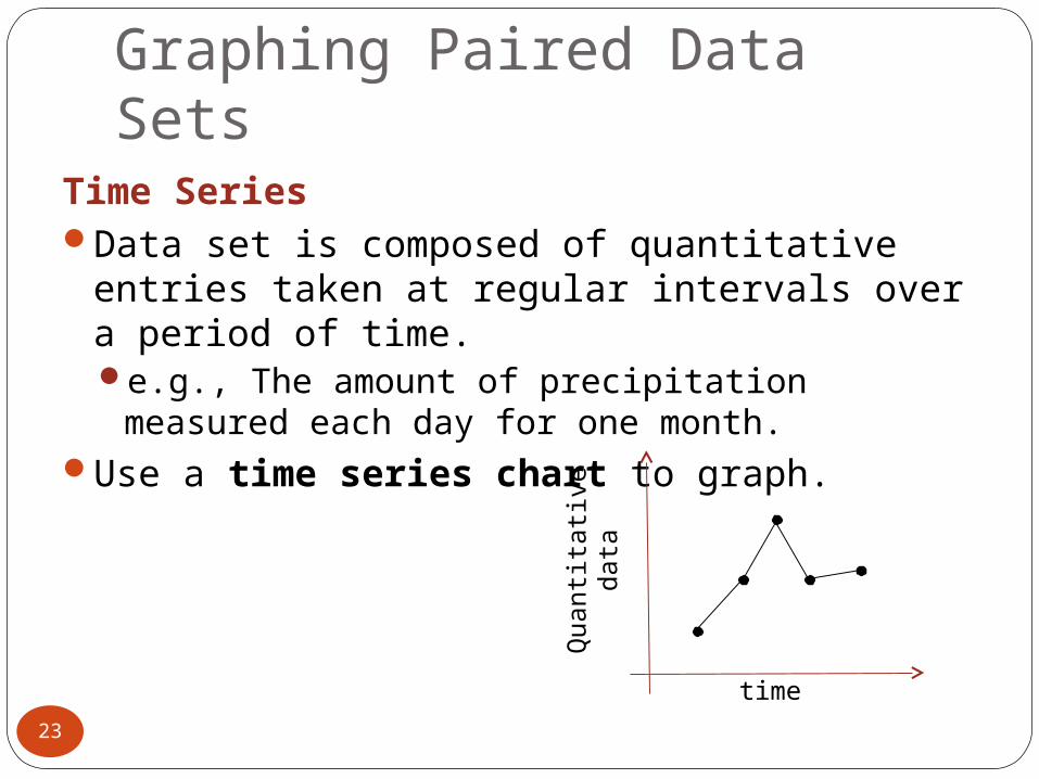
Graphing Paired Data SetsTime SeriesData set is composed of quantitative entries

taken at regular intervals over a period of time. e.g., The amount of precipitation measured

each day for one month. Use a time series chart to graph.

time

Quanti

tati

ve

data

23

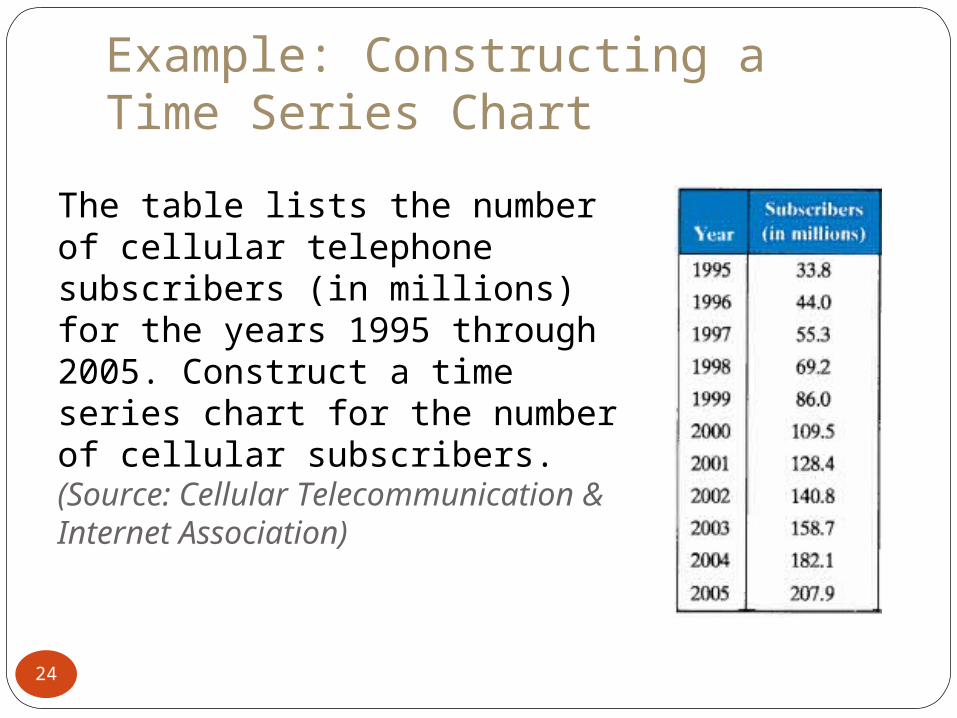
Example: Constructing a Time Series Chart

The table lists the number of cellular telephone subscribers (in millions) for the years 1995 through 2005. Construct a time series chart for the number of cellular subscribers. (Source: Cellular Telecommunication & Internet Association)

24

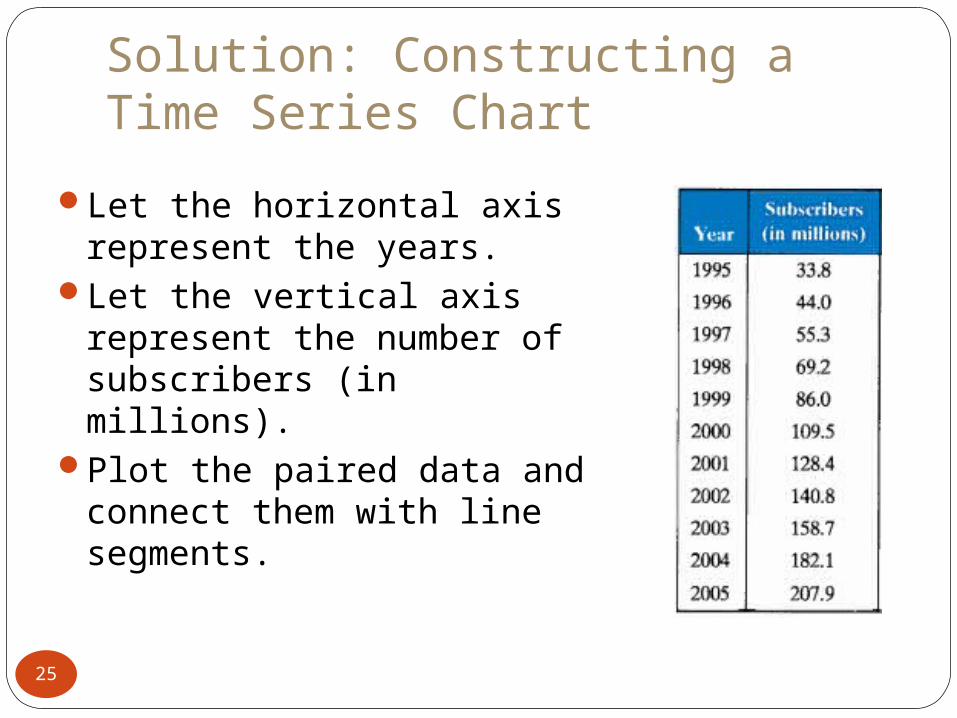
Solution: Constructing a Time Series Chart

Let the horizontal axis represent the years.

Let the vertical axis represent the number of subscribers (in millions).

Plot the paired data and connect them with line segments.

25

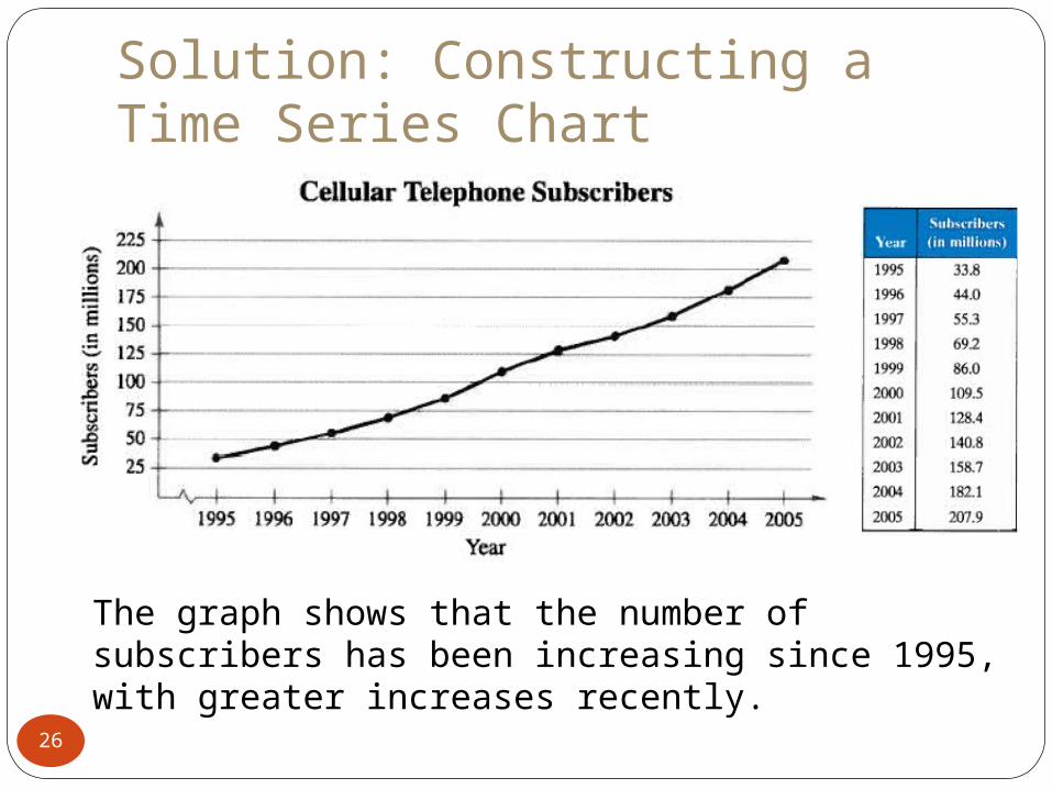
Solution: Constructing a Time Series Chart

The graph shows that the number of subscribers has been increasing since 1995, with greater increases recently.

26

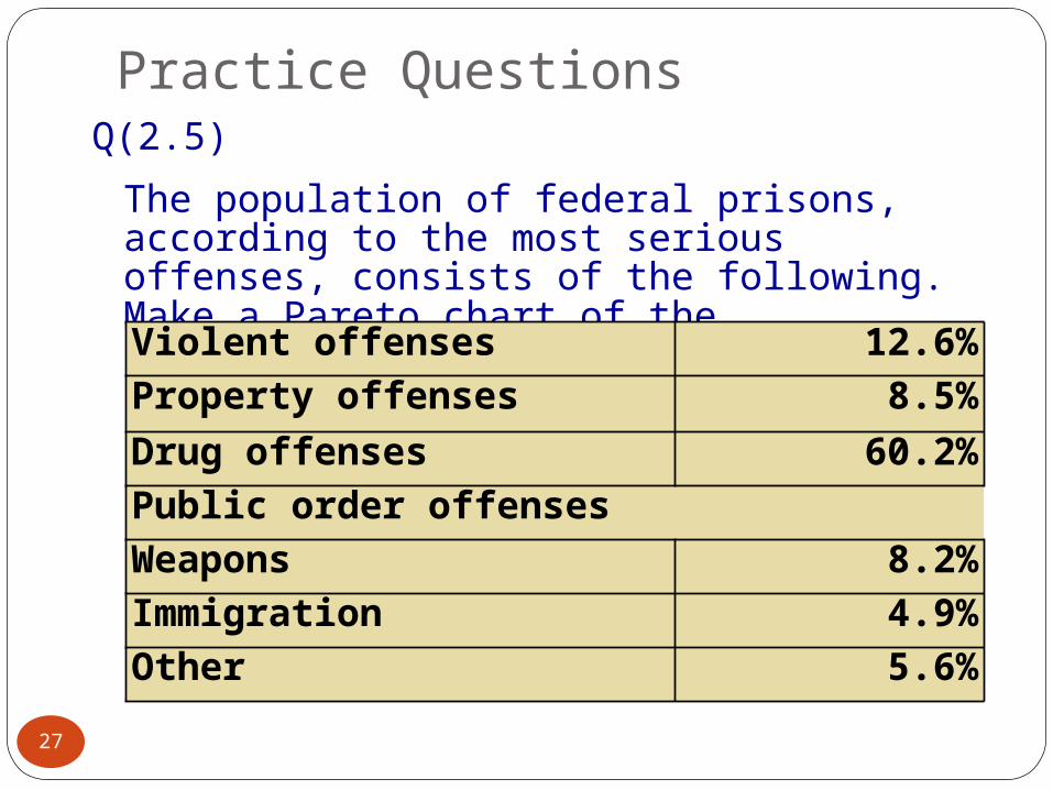
Q(2.5)

The population of federal prisons, according to the most serious offenses, consists of the following. Make a Pareto chart of the population.

27

Practice Questions

Violent offenses 12.6%

Property offenses 8.5%

Drug offenses 60.2%

Public order offensesWeapons 8.2%

Immigration 4.9%Other 5.6%

Q(2.6)

The assets of the richest 1% of Americans are distributed as follows. Make a pie chart for the percentages.

28

Practice Questions

Principal residence 7.8%

Liquid assets 5.0%

Pension accounts 6.9%

Stock, mutual funds, and personal trusts 31.6%

Businesses and other real estate 46.9%

Miscellaneous 1.8%

Q(2.7)

The age at inauguration for each U.S. President is shown below. Construct a stem and leaf plot and analyze the data.

29

Practice Questions

57 54 52 55 51 5661 68 56 55 54 6157 51 46 54 51 5257 49 54 42 60 6958 64 49 51 62 64

57 48 50 56 43 46

61 65 47 55 55 54

Q(2.8)

The data represent the personal consumption (in billions of dollars) for tobacco in the United States. Draw a time series graph for the data and explain the trend.

30

Practice Questions

Year 1995 1996 1997 1998 1999 2000 2001 2002

Amount 8.5 8.7 9.0 9.3 9.6 9.9 10.2 10.4

Section 2.2 SummaryGraphed quantitative data using stem-and-

leaf plots and dot plotsGraphed qualitative data using pie charts

and Pareto chartsGraphed paired data sets using scatter

plots and time series charts

31