Monterey, California management issues can now be evaluated in an experimental setting which eliminates the financial risks. The objective of the thesisi is to use the Sytems Dynamic

AD-A245 063

NAVAL POSTGRADUATE SCHOOLMonterey, California

DTIC0 GilAVU S ' LECT IFJAN2B 1992U

THESISDECISION MAKING FOR SOFTWARE PROJECT

MANAGEMENT IN A MULTI-PROJECT ENVIRONMENT:AN EXPERIMENTAL INVESTIGATION

by

Michael J. Hardebeck

September, 1991

Thesis Advisor: Tarek K. Abdel-Hamid

Approved for public release; distribution is unlimited

92-02117,-' 1 11

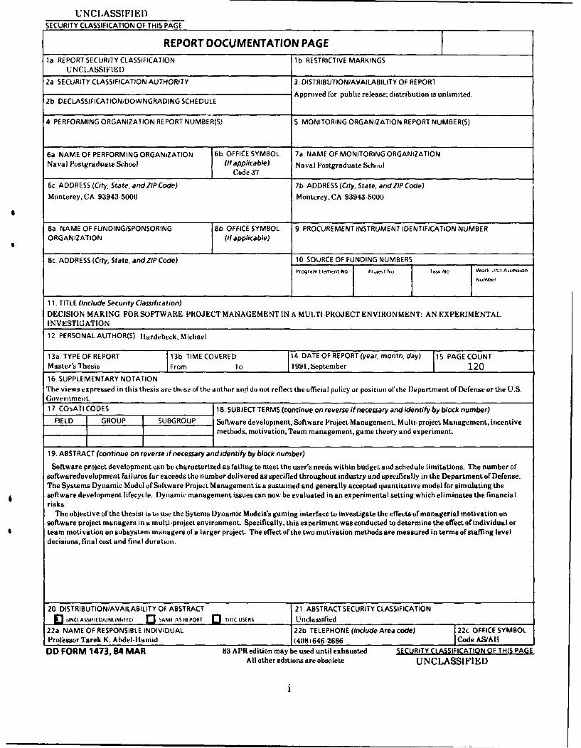
UNCLASSIFIEI)SECURITY CLASSIFICATION OF THIS PAGE

REPORT DOCUMENTATION PAGEla REPORT SECURITY CLASSIFICATION l b RESTRICTIVE MARKINGS

UNCLASSIFIED

2a SECURITY CLASSIFICATION AUTHORITY 3 DISTRIBUTION/AVAILABILITY OF REPORT

Approved for public release; distribution is unlimited.2b DECLASSIFICATIONIDOWNGRADING SCHEDULE

4 PERFORMING ORGANIZATION REPORT NUMBER(S) 5 MONITORING ORGANIZATION REPORT NUMBER(S)

6a NAME OF PERFORMING ORGANIZATION 6b. OFFICE SYMBOL 7a NAME OF MONITORING ORGANIZATIONNaval Postgraduate School (If applicable) Naval Postgraduate School

I Code 37

6c ADDRESS (Cty, State, and ZIP Code) 7b ADDRESS (City, State, and ZIP Code)Monterey, CA 93943-5000 Monterey, CA 93943-5000

8a NAME OF FUNDING/SPONSORING 1 8b. OFFICE SYMBOL 9 PROCUREMENT INSTRUMENT IDENTIFICATION NUMBERORGANIZATION (If applicable)

8c ADDRESS (City, State, and ZIP Code) 10 SOURCE OF FUNDING NUMBERSProgrdm ti ement NyO lPr.je. N. I dok No WorN UNIS AC ,n

humbr

11. TITLE (Include Security Classification)

DECISION MAKING FOR SOFTWARE PROJECT MANAGEMENT IN A MULTI-PROJECT ENVIRONMENT: AN EXPERIMENTALINVESTIGATION

12 PERSONAL AUTHOR(S) Hardebeck, Michael

13a TYPE OF REPORT 13b TIME COVERED 14 DATE OF REPORT (year, month, day) 15 PAGECOUNT

Master's Thesis From To 1991, September 12016. SUPPLEMENTARY NOTATIONThe views expressed in this thesis are those of the author antd do not reflect the official policy or position of the Department of Defense or the U.S.Government.17, CObATI CODES 18. SUBJECT TERMS (continue on reverse if necessary and identify by block number)

FIELD GROUP SUBGROUP Software development, Software Project Management, Multi-project Management, incentivemethods, motivation, Team management, game theory and experiment.

19. ABSTRACT (continue on reverse if necessary and identify by block number)

Software project development can be characterized as failing to meet the user's needs within budget and schedule limitations. The number ofsoftwaredevelopment failures far exceeds the number delivered as specified throughout industry and specifically in the Department of Defense.The Systems Dynamic Model of Sottware Project Management is a sustained and generally accepted quantitative model for simulating thesoftware development lifecycle. Dynamic management issues can now be evaluated in an experimental setting which eliminates the financialrisks.

The objective of the thesisi is to use the Sytems Dynamic Models's gaming interface to investigate the effects of managerial motivation onsoftware project managers in a multi-project environment. Specifically, this experiment was conducted to determine the effect of individual orteam motivation on subsystem managers of a larger project. The effect of the two motivation methods are measured in terms of staffing leveldecisions, final cost and final duration.

20 DISTRIBUTION/AVAILABILITY OF ABSTRACT 21 ABSTRACT SECURITY CLASSIFICATIONNCASSIFIED/UNLIMID 13 SAW AS 10.PORT 13DIC USERS Unclassified

22a NAME OF RESPONSIBLE INDIVIDUAL 22b TELEPHONE (Include Area code) 22c OFFICE SYMBOLProfessor Tarek K. Ahdel-|iamid (408)646-2686 Code AS/AH

DD FORM 1473,84 MAR 83 APR edition may be used until exhausted SECURITY CLASSIFICATION OF THIS PAGEAll other editions are obsolete U NC LASSIFI ED

i

Approved for public release; distribution is unlimited.

Decision Making for For Software ProjectManagement in a Multi-Project Environment:

An Experimental Investigation

by

Michael J. HardebeckLieutenant, United States Navy

B.S., The University of Texas, Austin, 1983

Submitted in partial fulfillmentof the requirements for the degree of

MASTER OF SCIENCE IN INFORMATION SYSTEMS

from the

NAVAL POSTGRADUATE SCHOOLSEPTEMBER 1991

Author: LMic ael J. Hardebeck

Approved by::_Tarek K. Abdel-Hamid, Thesis Advisor

Kishore Sengupta, Second R a

David R. Whipple, ChairmanDepartment of Administrative Scences

ii

ABSTRACT

Software project development can be characterized as failing to meet the user's needs

within budget and schedule limitations. The number of software development failures

far exceeds the number delivered as specified throughout industry and specifically in the

Department of Defense. The System Dynamics Model of Software Project Management is

a sustained and generally accepted quantitative model for simulating the software

development lifecycle. Dynamic management issues can now be evaluated in an

experimental setting which eliminates the financial risks.

The objective of this thesis is to use the System Dynamics Model's gaming interface

to investigate the effects of managerial motivation on software project managers in a multi-

project environment. Specifically, this experiment was conducted to determine the effect

of individual or team motivation on subsystem managers of a larger project. The effect of

the two motivation methods are measured in terms of staffing level decisions, final cost

and final duration.

'i

TABLE OF CONTENTS

I. INTRODUCTION . . . . . . . . . . . . . . . . . . . 1

A. BACKGROUND.....................1

B. PURPOSE OF RESEARCH.................4

C. SCOPE OF RESEARCH..................5

D. ASSUMP~TIONS.....................6

E. THESIS ORGANIZATION.................7

II. PREPARING THE GAMING INTERFACE.............8

A. EXPERIMENTAL DESIGN.................8

B. THE SOFTWARE...................14

C. THE DOCUMENTATION.................21

D. THE TRIAL EXPERIMENT................26

E. FINAL PREPARATIONS................30

III. CONDUCTING THE EXPERIMENT..............32

A. TASKS AND PROJECT CHARACTERISTICS.........32

B. ORGANIZING THE EXPERIMENT.............33

C. THE SAMPLE POPULATION...............35

D. DEPENDENT MEASURES................37

IV. EXPERIMENTAL RESULTS AND ANALYSIS..........41

A. MODEL OF ANALYSIS..................41

iv

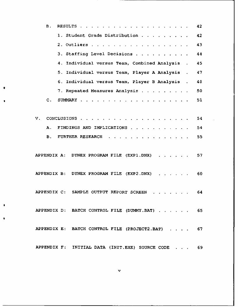
B. RESULTS ........ .................... 42

1. Student Grade Distribution .. ......... 42

2. Outliers ....... .................. 43

3. Staffing Level Decisions ... .......... 44

4. Individual versus Team, Combined Analysis 45

5. Individual versus Team, Player A Analysis 47

6. Individual versus Team, Player B Analysis 48

7. Repeated Measures Analysis .. ......... 50

C. SUMMARY ........ .................... 51

V. CONCLUSIONS ........ .................... 54

A. FINDINGS AND IMPLICATIONS ... ........... 54

B. FURTHER RESEARCH ...... ............... 55

APPENDIX A: DYNEX PROGRAM FILE (EXP1.DNX) ...... 57

APPENDIX B: DYNEX PROGRAM FILE (EXP2.DNX) ...... 60

APPENDIX C: SAMPLE OUTPUT REPORT SCREEN . ....... 64

APPENDIX D: BATCH CONTROL FILE (DUMMY.BAT) ...... 65

APPENDIX E: BATCH CONTROL FILE (PROJECT2.BAT) . . . . 67

APPENDIX F: INITIAL DATA (INIT.EXE) SOURCE CODE . . . 69

v

APPENDIX G: DATA STRIPPING (INFOOFB.EXE) SOURCE CODE 71

APPENDIX H: MULTI-PROJECT EXPERIMENT COMPUTER SCREENS 75

APPENDIX I: "DUMMY" EXPERIMENT DOCUMENTATION ..... 82

APPENDIX J: "PROJECT 2" EXPERIMENT DOCUMENTATION . 88

APPENDIX K: "PROJECT 2" DOCUMENTATION SHEET (PLAYER B) 94

APPENDIX L: SAMPLE POPULATION RANDOMIZING WORKSHEET 95

APPENDIX M: "PROJECT 2" EXPERIMENT PAIRS ........ 97

APPENDIX N: SEATING CHART ..... .............. 99

APPENDIX 0: STAFFING LEVEL DECISIONS SPREADSHEET . . . 100

APPENDIX P: SAMPLE DATA VALIDATION RUN .. ........ 101

APPENDIX Q: SAS DATA FILES ..... .............. 102

APPENDIX R: SAS CONTROL FILES .... ............ 106

LIST OF REFERENCES ........ .................. 110

vi

INITIAL DISTRIBUTION LIST.............. . . .. .. .... 1

ell,

IAccession ForNTIS GA&I mo

DTICT A0

p-El

vii,

£

B

I. INTRODUCTION

A. BACKGROUND

In a recent congressional report, eight major computer

systems in the U.S. Department of Defense experienced a

combined cost overrun of more than one billion dollars.

Further, a survey of software applications revealed that 47%

of the software applications were delivered and not used, 29%

were paid for but not delivered, 19% were abandoned or

reworked, and only 2% were used as delivered. In spite of

best efforts to reverse the trend of software project

development malaise, software systems continue to be delivered

late with cost overruns, poor reliability and user

dissatisfaction [Ref. 2: p. 1426). [Ref. 1]

The problem is compounded as the demand for software

applications continues to exceed the ability of many software

engineers to provide economical products on time that meet the

user requirements. A conservative estimate indicates a one

hundredfold increase in demand for software in the last two

decades [Ref. 2: p. 1426]. There is little argument that

technology has kept pace with the demand. Recent efforts for

improving performance have shifted the focus from the

technological production of the software application to the

managerial operating process and environment involved.

1

Managing software development is a very complex process.

The software project manager must make decisions based on a

wide variety of decision variables in an increasingly

competitive environment of scarce resources. A major

deficiency in much of the research to date on software project

management has been the inability to utilize our knowledge of

the microcomponents of the software development process such

as scheduling, productivity, and staffing to drive

implications about the behavior of the total socio-technical

system [Ref. 2: p. 1428].

The Systems Dynamic Model (SDM) of Software Project

Management represents a comprehensive model of the dynamics of

software development [Ref. 2: p. 1426]. Through the use of

the model, a wide range of managerial processes and dynamic

operating environments can be simulated, tested and evaluated.

The SDM has supported a stream of research into the

implications of managerial decision making in software

development projects. A stated benefit of using the SDM is

the ability to examine the effects of changing one factor

while all the other factors are held unchanged [Ref. 2: p.

1433]. The model was initially designed to evaluate such

factors as the effects of staffing level decisions on the

final cost and schedule in a single project environment.

Subsequent enhancements to the model expands its capabilities

from single project simulation to multiple project or

subsystem simulation environments.

2

This enhancement offers a rich opportunity to evaluate the

dynamics of decision making in a multi-project environment.

Using a number of project managers operating as pairs, data on

many potential software project management concerns and

general management theories can be evaluated. Such potential

questions include: subsystems of a larger project with

overlapping start dates, differing or competing resources, and

changes in project size and/or complexity. Pert charts

traditionally identify a single critical path; however, with

modular software development there may be several critical

paths de7ending on changes in a subsystem's complexity. The

enhanced SDM might be used as an iterative process for

optimizing this situation.

An area of significant concern in a time of decreasing

budgets and increasing oversight is managerial decision making

with insufficient resources. An interesting issue is the

motivation style employed to ensure the performance of two

subsystem managers operating on a single project with a

limited resource pool of staff. One alternative motivation

method is to reward or compensate managers based on the

performance of their subsystem. This puts them in direct

competition with their counterpart. The other motivation

method, in this case, is to reward or compensate managers

based on the total performance for the combined project. This

is "team" motivation versus "individual" motivation and is

intuitively the preferred management style. The question is,

3

does team motivation produce improved results as measured by

the final cost and final completion date of the project as a

whole?

B. PURPOSE OF RESEARCH

The purpose of this thesis is to design, construct and

execute a multi-project management experiment, using the

enhanced version of the SDM gaming interface. This experiment

addresses the research question of the effects of managerial

motivation on project performance. Even though "individual"

versus "team" motivation has been explored in general

management theory, it has not been formally tested with

respect to software project development. A review of the

literature with respect to competition and incentives has

revealed very little research conducted to identify an

acceptable experimental format under these circumstances. The

software project management system is a far more complex

conglomerate of interdependent variables that are interrelated

in various nonlinear fashions (Ref. 2: p. 1427].

The SDM gaming interface is used to present management

pairs with a standard interface to the simulation model. The

managers are subject to either "team" or "individual"

motivation and are required to make staffing level decisions

through the design and testing phases of project development.

Performance is measured in terms of final cost and final

completion date of the total project. This data is analyzed

4

using standard SAS procedures to determine the significance of

performance deviation. Through this process, some light

should be shed on management motivation in multi-project

environments.

Secondly, this thesis is intended to be a model for

conducting experiments using the SDM gaming interface. The

multi-project experiment serves as the context for presenting

a sequential series of steps taken to design and conduct the

experiment as well as analyze the data. In general, sections

are written with the methodology-specific information

preceding the experiment-specific information.

C. SCOPE OF RESEARCH

The scope of this research includes the design,

construction, preparation of documentation and software,

execution and data analysis of the multi-project experiment.

The design required an iterative process of diagraming,

building and testing several potential models in order to

identify the single independent variable that offered the

richest research opportunity. The construction of the

experiment required that the SDM model gaming interface be

tailored for the specific research question. Special care was

taken in the presentation of the interface and reports to the

experimental subjects in order to prevent introducing any

external biases that could affect the results. The

preparation of the experiment entailed writing the

5

documentation that each group used and finalizing the files

required by each experimental group onto a single floppy disk.

Each experimental subject was presented with an individual

folder and any specific instructions. The execution of the

experiment was organized to conduct and collect the data in a

single day. This was accomplished with two groups of roughly

thirty subjects each. Limitations on scheduling and

microcomputer resources dictated such careful planning. The

analysis of the data consisted of analyzing the data with

Quattro Pro spreadsheet software and SAS statistical system

procedures.

D. ASSUMPTIONS

The subjects in this experiment were fifth-quarter (in a

six-quarter curriculum) graduate students studying in the

Computer Systems Management curriculum at the Naval

Postgraduate School. These same subjects participated in a

similar experiment using the SDM gaming interface during

previous quarters. Although the subjects were not practicing

software project managers, the amount of training completed in

the curriculum and experience with similar software management

experiments leads to the assumption that the results of the

experiment and the conclusions would be represented in the

software industry. This is also supported by the work of

William Remus [Ref. 3:pp. 19-25].

6

E. THESIS ORGANIZATION

Chapter II is a description of the software files and

documentation design and construction considerations in

preparing the experiment materials. The chapter also includes

a section on conducting the trial experiment. Chapter III is

an in-depth description of the methodology, sample population,

and experiment organization required to conduct the

I experiment. Chapter IV validates and analyzes the

experimental results. Chapter V summarizes the significant

accomplishments and implications of the findings presented in

Chapters II-IV and provides recommendations for further

research.

7

II. PREPARING THE GAMING INTERFACE

A. EXPERIMENTAL DESIGN

The Systems Dynamic Model gaming interface enables

software management experiments to be designed which are

similar in many ways to the flight simulators that pilots use

to mimic flying an aircraft from takeoff at point A to landing

at point B. Instead of flying an aircraft, though, this

simulation mimics the life of a real software project from the

start of the "design" phase until the end of the "testing"

phase. Virtually any management concern or theory can be

tested by designing an appropriate experiment and gaming

interface. Figure 2-1 is a simple experimental design

worksheet used to conceptualize many design possibilities.

Exploratory experimental designs and test simulations

using the gaming interface, as well as the ideas presented in

previous research with the SDM gaming interface, provided

several potential research questions. While a single research

question was isolated for examination, some of the most

interesting alternative questions are described in Chapter V.

In a time of decreasing budgets and increasing oversight

the richest research opportunity is managerial decision making

with insufficient resources. An interesting issue is the

motivation method employed to ensure the performance of two

8

subsystem managers operating on a single project with a

limited resource pool of staff. By imposing a restrictive

workforce ceiling, real life concerns can be addressed. One

alternative motivation method is to reward or compensate

managers based on the performance of their subsystem. This

puts them in direct competition with their counterpart. The

other motivation method, in this case, is to reward or

compensate managers based on the total performance for the

combined project. This is "team" motivation versus

"individual" motivation and is intuitively the preferred

management method. The question is, does team motivation

produce improved results as measured by the final cost and

final completion date of the project as a whole?

Figure 2-1 is the worksheet representation of the

experimental design of this thesis. In this experiment,

subjects play an important role as the manager of one of two

major subsystems that are being developed on a single project.

Subjects were paired as the two subsystem managers for the

project. Each subsystem manager was required to track the

progress of his subsystem using a number of status reports

that were produced at two-month intervals (40 working days).

As the subsystem manager, the subject was required to

determine and/or revise the staff size required for his

subsystem at each reporting period. When entering staffing

level decisions at each time period, subjects were required to

coordinate with the other subsystem manager to ensure that

9

their total staffing needs did not exceed the imposed staff

level ceiling for the project as a whole. Each subject

MULTIPROJECT EXPERIMENT

RESOURCECOMPET1ON TEAM INDEPENDANT

FORSCARCERESOURCES 20% - 80% 80% - 20%

PLAYERA

GROUP GROUP

WFNTRI(1) AT AI

INCREASEDPROJECT

SIZE

PLAYERB GROUP GROUP

WFNTRI(2) BT BI

INCREASEDCOMPLEXITY

Figure 2-1 Experimental Design Worksheet

entered into the simulation his and the other subsystem

staffing level needs.

10

Subject pairs were divided into two sets according to the

method of motivation imposed. While the subjects were not

monetarily compensated for their efforts, they were told that

their performance would impact their assigned grade in the

Software Engineering course they were taking. This ensured

that the subjects provided a serious and diligent effort. One

set was given written instructions which indicated that 80% of

their compensation would depend on the performance of their

subsystem with only 20% compensation for the performance of

the overall project. This set is referred to as

"Individually" motivated. The other set was given written

instructions which indicated their compensation would be 80%

for the performance of the overall project and only 20%

compensation for the individual subsystem performance. This

set is referred to as "Team" motivated. Pairs consisted of

Player A and Player B, both receiving written instructions of

the same motivation method. The performance of the "Team"

motivated Player A and Player B pairs was compared to the

performance of the "Individually" motivated Player A and

Player B pairs.

The independent variable is the method of motivation and

the dependent variables include: final cost, final schedule

and staffing level decisions.

One experimental concern was that the pairs would simply

compromise rather than compete for staff resources by dividing

the available pool down the middle. This issue was resolved

11

by altering the dynamics of each subsystem. The Player A

subsystem increased in number of tasks roughly double during

the life of the design and testing phases. The Player B

subsystem increased in complexity roughly double during the

life of the design and testing phases. Each subsystem,

therefore, experienced an increasing need for staff. Further,

each subsystem was staffed with an initial core team of five

people remaining at the end of the requirements phase.

The result was four groups of subjects who received group-

specific sets of instructions. The groups are referred to as

"AI" (indicating Player A, Individually motivated), "AT,"

"BI," and "BT," as indicated in Appendix A.

The experimental population had previous experience with

the SDM gaming interface within the previous six months. In

order to prepare the subjects for providing the best possible

performance, each subject received an initial 30 minute review

of the function of the gaming interface. During this initial

review the subjects were reminded that a real project

management situation did not provide them with absolute

control over the work force level. Turnover, promotions, work

force ceilings, transfers, hiring and assimilation delays

prevent the manager from always getting the exact work force

requested. Following the review session, each subject

performed a "DUMMY" simulation on an individual basis. This

design and documentation is discussed later in this chapter.

The purpose of these training sessions was to eliminate any

12

discomfort, unfamiliarity or bias that might be attributed to

subject interaction with the gaming interface itself. Only on

the day of the experiment were the subjects informed of the

subsystem nature of the experimental task and that they would

be paired with a randomly-selected counterpart.

The DUMMY simulation was a SDM model named EXPI based on

an actual NASA experiment. Each subject played this

simulation as a single project, entering the desired work

force level required. The input variable named WFNTR1(1) was

transparent to the subjects. Each subject played the

simulation for two forty-day time periods (80 days) to become

familiar with the interface and then exited out of the

program.

The actual experiment was a SDM model named EXP2 based on

an actual NASA experiment which has been used as the basis for

several other research experiments. By using the real

projects with real data, the results of the experiment can be

measured, compared and validated against a known baseline.

Each subject was required to enter, for each time period, the

desired staff level for his subsystem as well as for his

counterpart's subsystem. A simple computer algorithm

prevented the subjects from entering a combined total greater

than the imposed work force ceiling levels for the project as

a whole.

13

B. THE SOFTWARE

In order to conduct the experiment, two significant design

and construction efforts were required so that the

experimental subjects experienced the design outlined above.

The first was the construction of the software which drives

the computer gaming interface that the subjects used. The

second was the documentation which explained to the

experimental subjects the instructions, environment, task,

rules and other considerations. This documentation was also

used to capture in writing the desired staffing level

decisions.

The SDM model gaming interface includes the Dynamo

simulation files as well as the Dynex files which allow the

model designer to interface with the Dynamo simulation

language. The objective is to assimilate a set of files whose

construction allows the novice user (experimental subject) to

simply start and play the gaming interface with ease and

without error. Further, the files must be designed in a

manner which allows the designer to capture the raw data for

further analysis. While the actual contents of the base file

set may differ depending on the experimental design in

question, there is a minimum of 13 files required to provide

a format for a smooth gaming interface design. Figure 2-2 is

the base file set used for this experiment.

The Dynamo simulation model should be constructed,

modified and maintained by a single project manager. This

14

model controls all the dynamic variables which define the

experimental setting. The base set files EXP2.DAT, EXP2.INS,

and EXP.SMT are the minimum required files that define the

project environment. The only limitation with these files is

that all the variable names used with the remainder of the

base set of files must be defined within these Dynamo files

prior to their compilation.

MOVE.BAT Transfers output files to a floppy.PROJECT2.BAT Control file for experiment.BAT.COM Batch enhancement language.EXP2.DAT Dynamo required data file.EXP2.DNX Designer Dynex interface to Dynamo.EXP2.DRS Output report specification.DYNEX.EXE Dynex execution file.INFOOFB.EXE C language data stripping file.INIT.EXE C language initializing file.REP.EXE Report generator execution file.SMLT.EXE Dynamo simulation execution file.EXP2.INS Dynamo required simulation file.EXP2.SMT Dynamo required simulation file.

Figure 2-2 Base File Set

The language interface that the experiment designer will

use to interact with the Dynamo model is called Dynex [Ref.

4]. The Dynex file EXPI.DNX (filename.DNX) for the DUMMY

simulation is included as Appendix A, and the Dynex file

EXP2.DNX for the experiment simulation is included as Appendix

B. These files are written by the experiment designer and are

plain ASCII text which can be edited with a favorite text

15

editor, even WordPerfect. Chapters 12 and 13 of the Dynex

user's manual (Ref. 4] provide the basic instructions for

constructing the Dynex file. The basic purpose of this file

is threefold: to provide dialog to the user which identifies

what the user needs to do to interact with the gaming

interface, to capture the variable(s) required for the

simulation, and to provide a report format for the output

screens. In the case of the DUMMY simulation the user was

instructed to enter a single staffing level decision

(WFNTR1 (1)). In the case of the experiment simulation the

user was instructed to enter the staffing level decision for

Player A's subsystem (WFNTR1(1)) and Player B's subsystem

(WFNTR1 (2)). In order to personalize and standardize the

gaming interface for all subjects, the order of appearance of

the variables in EXP2.DNX were ordered such that each player's

staffing level input was solicited first. The order of

appearance of WFNTR1(1) and WFNTR1(2) in Appendix B reflects

the Dynex file used for all Player A subjects. The reverse

order was used for all Player B subjects.

The Dynex file was further personalized in the reporting

format of the output screen. Notice that each of the report

variables appearing at the end of EXP2.DNX specify 1 in

parenthesis corresponding to the use of WFNTRl(1) for Player

A. Likewise Player B received a report output screen which

specified only the variables corresponding to WFNTRI (2). This

produced an output report at the end of each simulated time

16

period which showed only the status of the individual

subsystem. In this manner, each subject was able to keep his

subsystem status confidential. A sample output report screen

is included as Appendix C. In addition to the output report

specification at the end of the Dynex file, this output report

specification also should be duplicated in a file by itself

with a .DRS extension, as is the case with the base set file

EXP2.DRS. This file is used by the Dynamo simulation model to

specify and record the output format.

The second file that is directly controlled by the

experiment designer is the batch control file which controls

the flow of the gaming interface. The file DUMMY.BAT is

included as Appendix D for the DUMMY simulation and the file

PROJECT2.BAT is included as Appendix E for the experiment

simulation. This is a standard batch file routine which

controls the traffic fiow while playing the game. The most

noteworthy feature of these batch files is that they allow

full use of the computer screen. Depending on the text editor

used, this file may not reflect the true appearance of the

screen until it is executed. Notice that the batch file

controls the order of program execution, as well as

controlling screen colors and menu selection options. The

batch files used in this experiment were enhanced using the

Extended Batch Language (EBL) to control menu selection items

and appear in the base set of files as BAT.COM. While EBL was

used in this experiment there are several alternative

17

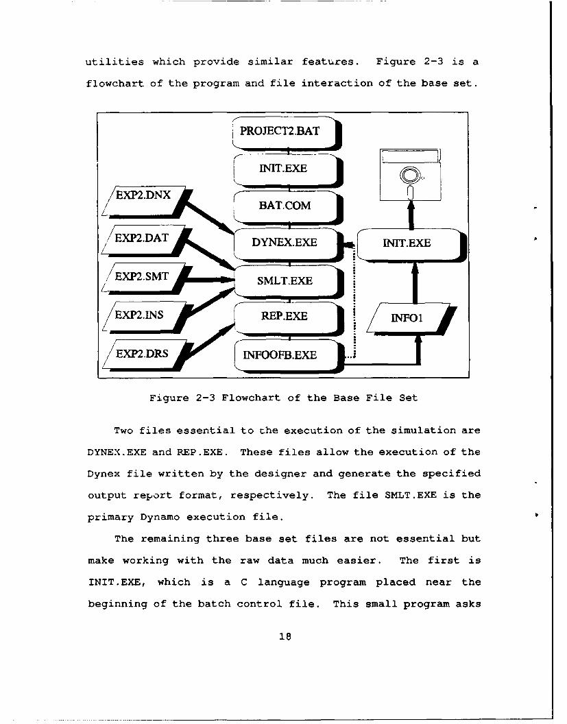
utilities which provide similar features. Figure 2-3 is a

flowchart of the program and file interaction of the base set.

EX2.N DBE.E NI.E

SMLT.EX i

,iEXP.DRS NOF-EX

Figure 2-3 Flowchart of the Base File Set

Two files essential to the execution of the simulation are

DYNEX.EXE and REP.EXE. These files allow the execution of the

Dynex file written by the designer and generate the specified

output report format, respectively. The file SMLT.EXE is the

primary Dynamo execution file.

The remaining three base set files are not essential but

make working with the raw data much easier. The first is

INIT.EXE, which is a C language program placed near the

beginning of the batch control file. This small program asks

18

the experimental subject to enter his name and Student Mailbox

Code (SMC). The program also captures the keystrokes that the

subject enters during the course of the experiment which can

be used as an audit trail. This data is deposited in a file

called LOG1. The source code for this program is provided as

Appendix F. The second base set file is INFOOFB.EXE, also a

C language program, which reads the numerical data values from

their video screen position and strips the data values from

each output report screen. Appendix C is a sample output

screen. This program reads the data displayed for each time

period as recorded in the JUNK.OUT output file described

later. INFOOFB.EXE can and must be specifically modified and

compiled to match each text report used. The system designer

should place the INFOOFB.EXE program call in the controlling

batch file, just after the REP.EXE program call. This type of

file can be used to record the output data from several

different text report screens by modifying the source code

(provided in Appendix G), changing the program name and

changing the destination file name. This is a time-saving

program which collects all the report data and deposits it

into a file called INFOl The third base set file is MOVE.BAT

which is a simple batch file written to transfer the output

files and the data files described about from the C: hard

drive directory to a floppy diskette in the A: drive. The

necessity for this file is described in Chapter III.

19

When the simulation is executed these 13 files expand to

a total of 22. The additional files that are created by the

Dynamo simulation are presented in Figure 2-4.

INFOl Data stripped from INFOOFB.EXELOG1 . Data recorded by INIT.EXEEXP2.CHG Dynamo generated file.EXP2.OUT Complete report log.INTERVAL.OUT Holds the last report output screen.JUNK.OUT INTERVAL.OUT, but Feeds INFOOFB.EXE.EXP2.RSL . Dynamo generated file.EXP2.STT . Dynamo generated file.EXP2.WAS Temporary store for input variables.

Figure 2-4 Dynamo Created Simulation Files

The INFOl and LOG1 files are described above and are

useful during data validation and analysis. All the .OUT

files, including JUNK.OUT, provide the reported results from

the output report screen. Depending on the research question,

this information may be used to evaluate many alternative

issues. The EXP2.WAS file temporarily records the Dynex input

variable values of WFNTR1(1) and WFNTR1(2). During the next

iteration, the Dynex file recalls these values and reports

them as the last recorded entries. The new variable values

replace the old ones. Appendix H is a copy of each of the

computer screens, in sequence, which is the product of

programming the software. These screens are the actual ones

seen by the subjects during the experiment.

20

The software for the DUMMY experiment was designed and

constructed to represent the experiment environment as closely

as possible and still remain in a single project mode. The

primary intent of the DUMMY simulation was to familiarize the

subjects with the gaming interface. The experimentation

interface differed only where necessary to facilitate the two-

player option.

C. THE DOCUMENTATION

The documentation provided to each subject was an

instruction set which described the purpose, scope, rules and

procedure for the gaming interface. For the experimental

subject, the documentation was the key link in achieving a

clear understanding of his role in the experiment. For the

researcher, the documentation served two very important

functions: to give each subject any unique instructions, and

to capture the staffing level decisions.

The experimental sequence of events had the subjects

performing a DUMMY simulation two days prior to the actual day

of the experiment. As previously stated, the DUMMY simulation

was designed to be as closely identical to the actual

experiment as possible without revealing the nature of the

experiment to be conducted. As such, the documentation

provided to each subject closely followed the documentation

that was used for the experiment. Appendix I is a copy of the

DUMMY documentation set provided to each experimental subject.

21

The DUMMY documentation differs only in reference to single

versus multi-project environments and most significantly in

the area of compensation. The instructions for compensation

specified in the DUMMY documentation identify that the

performance criteria is strictly calculated as a function of

schedule and budget overruns. The experiment documentation

uses the same base calculation for performance; however, the

multi-project environment provides the opportunity to affect

the manager's motivation to perform.

When constructing both the computer interface and the

written instructions, it is important to eliminate any

external bias in the experiment environment. Unless the

research question is directly dependent on the gaming

interface itself (as is the case when evaluating feedback

models), the computer interface should be identical for each

subject. As a result, the documentation itself represents the

primary means to convey unique information to a subject. The

unique instructions for the experiment documentation appear on

the second page of Appendix J. Each subject was told that

his/her compensation was based on either 80% individual or 80%

combined performance. Appendix J is the unique set of

instructions provided to the "AI" group of subjects. This

designates that this Player A was independently motivated. In

the multi-project environment the method of motivation served

as the independent variable for this experiment. The section

titled "YOUR GRADE" identified to the subject the motivation

22

method in terms of the manner in which his performance would

be compensated. Figure 2-5 is the unique instruction that all

individually-motivated subjects received.

********************************************** *******

* IMPORTANT *

* 80% of your compensation will be based on your ** subsystem's performance. ** 20% of your compensation will be based on total ** project performance. ** *

Figure 2-5 Compensation Criteria for Individual Motivation

Figure 2-6 is the unique instruction that all team-

motivated subjects received.

************************ *

* IMPORTANT *

* 20% of your compensation will be based on your ** subsystem' s performance. ** 80% of your compensation will be based on total ** project performance. *

Figure 2-6 Compensation Criteria for Team Motivation

The 80-20 split was chosen as a realistic motivation

environment that may be employed in actual software

development management, where 100% in either direction may be

unrealistic.

23

Both the DUMMY and the experiment documentation identify

to the subject some important considerations. These

considerations include information on how the size of the full

time staff is dynamically affected by: work force ceiling,

hiring delays, assimilation time, and turnover rate. The

subjects were provided with clear instructions that they may

not exceed any imposed work force ceiling. A simple heuristic

for calculating a minimum staff level required at any

reporting period was also provided both by instruction and by

example. During the training session conducted on the day of

the DUMMY simulation it was stressed that this heuristic did

not take into account all the staff level dynamics identified

above, rather that they would also need to use their

judgement.

The documentation also includes a step-by-step set of

instructions on the exact keystroke sequence of events

required while using the computer gaming interface. At the

end of the training session and the DUMMY simulation, all

experimental subjects were interacting with the gaming

interface without error.

The final page of the documentation handout is the

staffing level record sheet. This page identifies to the

subjects the initial estimates for the size, cost, duration

and core team. The DUMMY documentation identified these

values for the single project being managed. The experimental

documentation identified these values for the subject's

24

subsystem and his counterpart's subsystem. Tasks roughly

represent 50 lines of code and the core team represents the

group of software professionals that developed the subsystem's

requirement specification. For Player A the initial size and

duration of the subsystem was specified as 396 tasks and 1,i1

man days, respectively. For Player B the initial size and

duration of the subsystem was specified as 475 tasks and 1,345

man days, respectively. The size of the initial core team was

set at five people. In order to provide consistency

throughout the experiment, the terms "Your Subsystem" and

"Other Subsystem" were used both in the documentation and in

the gaming interface. As such, the final page of the Player

B documentation reverses the order of appearance of the

initial estimate information. The final page of the Player B

documentation is provided as Appendix K. The Dynex gaming

interface was constructed to impose a work force ceiling of

fifteen for both subsystems combined, or the project as a

whole. Taking into account that the Player A subsystem

increased in size and the Player B subsystem increased in

complexity during the life of the project, and through several

trial simulations, a work force ceiling of 15 was determined

to be just barely enough to complete the two subsystems within

a reasonable budget and schedule.

The Dynex software uses a file called "filename.WAS" to

store temporarily the staffing level variables used by the

Dynamo simulation. With each iteration, this .WAS file is

25

overwritten and the information is lost. The record sheet is

therefore the only practical means to capture the staffing

level decisions. The only means to by-pass this limitation is

to include the staffing variables WFNTRl(1) and WFNTR1(2) in

the output report. This may or may not be desirable.

Validation of this written data is discussed in Chapter IV.

D. THE TRIAL EXPERIMENT

Once the gaming interface and the documentation have been

prepared, trial experiment(s) should be conducted to provide

the researcher with feedback on any potential design or

implementation problems. Two students who had knowledge of

the System Dynamics Model beyond that of the remaining sample

population were selected to play the experiment simulation as

a trial experiment or pilot study. The objective of the trial

experiment was not to measure the performance, but rather the

interaction of the students with the documentation and the

gaming interface. The following is the initial list of

objectives for conducting the trial experiment.

- Are the instructions clear?

- Do the subjects appear to be comfortable with theinterface?

- How long does the experiment take?

- How do the subjects interact with each other during theexperiment?

The trial experiment was conducted using the documentation and

interface for the multi-project experiment. At the time of

26

conducting the trial experiment a second research question was

under development and considered for inclusion as a second

experiment. This second research question would have had each

subject manage a single project similar to the DUMMY

experiment before completing the multi-project experiment.

Due to the time limitations, the potential for biasing the

subjects for the multi-project experiment and the following

findings of the trial experiment, the single project

experiment was dropped. The following is a long but not

comprehensive list of pertinent observations and lessons

learned as a result of conducting the trial experiment.

- Elapsed time 1 hour 40 minutes. Keeping in mind that thisexperiment will be preceded by a DUMMY experiment andPROJECT1, an estimated time range for all subjects wouldprobably be on the order of 2 to 3 hours. This could bea problem in terms of lab assets and attention span.

- Though time is limited, running DUMMY and PROJECT1 on oneday and PROJECT2 on another would ease the time pressureand ensure that the sample population is familiar with theinterface prior to running the multi-project experiment.

- Both subjects appeared to be seriously conscientious.

- They read the instructions carefully without anyquestions.

- They were careful not to divulge any information to theircounterpart.

- They complained initially about the simulation speedassociated with disk reads from the A drive but did notpersist once they accepted the conditions. The simulationseemed to run reliably from the A drive.

- Player B was very familiar with the model and immediatelytried to out-game the simulation.

- Both subjects spent a good deal of time studying theoutput report.

27

- Need to tell the sample population to bring calculators to

the simulation.

- Player B questioned if 40 days equals 2 working months.

- Both subjects spent an extraordinary amount of time tryingto solve the "optimal" COCOMO solution and appearedfrustrated with their attempts. As much time was spentwith a calculator and paper as with the entire rest of theexperiment. This consumed a tremendous amount of time andcould result in some subjects taking more time to completeall three project sets than the allotted time for the useof the labs.

- Player A noticed the increase in tasks after period 2 andexpressed some distress. At the end of the simulationPlayer B noticed that tasks had not increased yet progresstoward development dropped significantly following period4. Player B expressed that this was probably attributedto a decrease in personnel productivity and seemed veryupset that this was not measurable. Player B's projectstalled even though tasks did not change and staffing washigh. This subsystem was ultimately much higher in cost.

- Both subjects seemed to have become very familiar with theenvironment and would serve well as lab attendants.

- With Player A's subsystem having escalating tasks andPlayer B's subsystem having some dynamic change inproductivity, performance comparison seems to only bevalid in A to A and B to B vice A to B.

- Subject B calculated that the 50 lines of code per tasktimes the initial estimate of the number of tasks produceda number of lines of code which when entered into thebasic COCOMO formula did not match the initial staff sizeof 5 people.

- The only available explanation was that the LOC/Task is anapproximation and that the COCOMO calculations are tenuousin a dynamically-simulated environment.

- On the first time at the MAIN MENU screen, both subjectshit ENTER after selecting option one and returned to theMAIN MENU. This was never repeated as a problem once themechanics of the interface were understood.

- This researcher does propose that with one menu option itwould seem to make sense that the MAIN MENU screen is notneeded. This option has been investigated on apreliminary basis and is determined to be such an integral

28

component to the structure of the main batch file that anentirely new batch file structure would have to beadopted. This would probably take longer to change thanthe allotted time available.

- Researcher's note: If the variable which will serve asthe basis for statistical analysis is the staffing levelschosen then it would seem important to capture this dataelectronically vice depending on the documentation sheets.Several times the subjects were reminded to record theirdecisions on the documentation sheets. The only knownpossibility for this is to include the WFNTR1 for eachperiod in the status report ("Your Selected StaffSize...") and capture the .OUT files. Since the inputsare overwritten in the .WAS file the above option is theknown possibility.

- After period 4, Player B hit key 2 to proceed to the nextsimulation and could not return to view the status report.The experiment continued with Player B leaving thestaffing level for period 5 the same. This does notappear to have been a problem with previous research andwas not repeated as a mistake again. A loop at this pointmay be possible, but could take longer to program than theremaining time.

- Both subjects began reducing staff size by period 6. Ifconstrained resources is intended to be a researchenvironmental condition, then a max ceiling of 20 isrecommended with anything less (i.e., 15) increasing thepressure and influencing the outcome.

A quick scan of the above observahioiis indicates the

breadth and depth of information gleaned from the trial

experiment. This information proved invaluable in shaping the

content, structure and format for conducting the experiment.

The two students who participated in the trial experiment were

later used as lab attendants for the actual experiment.

29

E. FINAL PREPARATIONS

Having prepared the gaming interface and the documentation

for the multi-project experiment, the lessons learned from the

trial experiment produced a single research question: Whether

team motivated multi-project managers performed better than

individually motivated project managers. The work on the

gaming interface with modifications adopted as a result of the

trial experiment produced the clean base set of 13 files.

There were two versions of the base set. The Player A and

Player B versions of the software differed only in the Dynex

control file. The first difference is that the input

variables WFNTR1(1) for Player A and WFNTR1(2) for Player B

reverse order of appearance such tiiat the specified Player's

variable appeared first as "Your Subsystem" and the

counterpart variable appeared second as "Other Subsystem."

The second difference is in the report format at the end of

the Dynex file where all report variables use the (1) or (2)

subscripts depending on which Player's disk was specified.

Remember also that the PROJECT.DRS file duplicates the report

format and the associated subscripts. The identical Player A

or Player B set of files was used regardless of motivation

method specified in the documentation.

The final smooth copies of the documentation required a

unique set of instructions for each of the four groups: "AI,"

"AT," "BI," and "BT." Each of these sets of instructions

differed only in the compensation message on page two for

30

individual or team, and the order of the initial estimates on

the final page for Player A or Player B. The results of the

preparation produced a clean set of instructions and a single

floppy diskette for each unique subject group.

Other preparations included: verifying the scheduled

availability of the lab and sample population, preparing

lecture notes for the training session, and hardware

pretesting.

31

III. CONDUCTING THE EXPERIMENT

A. TASKS AND PROJECT CHARACTERISTICS

By completing the introductory training session and DUMMY

simulation two days prior to the day of the actual experiment,

the research subjects were familiar with the Dynamo gaming

interface and skills required to manage software projects.

Project two was the experiment simulation scenario

designed to address the research question. The simulation was

designed to allow the experimental subjects, working together

as management pairs, to make staffing level decisions for one

of two subsystems every forty days until the completion of

both projects. The subsystem manager acts as a resource

manager who must allocate his/her manpower resources as

necessary to complete the project on time (days) and on budget

(man days). Subjects used the gaming interface to enter the

staffing needs for the two subsystems and were provided with

an odtput report which provided the subjects with a status

report of their progress at intervals of forty days. This

status report was designed to be in a standard text format

which allowed the data in each output report to be captured by

the gaming interface. The final cost and schedule data were

then obtained for each individual and also for each managing

pair.

32

The staffing level decisions were entered into the gaming

interface as well as recorded on the final page of the

documentation sheet. Both subsystem staffing level decisions

were recorded as a measure of comparison.

Each student's participation grade in the Software

Engineering course was contingent on participation in the

simulation. This was used as an instrument to keep the

subjects motivated.

B. ORGANIZING THE EXPERIMENT

The experimental setting consisted of a ten-minute

classroom training session in which the nature, sequence of

events and instructions were verbally explained to the

subjects. The subjects moved from the classroom to one of two

preassigned labs down the hall. Each lab had 12 80286

personal computers. Each student had a folder sitting on the

keyboard of a preassigned PC with his or her name on it. In

order to avoid inadvertent sharing of status report

information, subjects were instructed to turn their monitors

so that they faced away from their counterparts. The

experiment was conducted in a single day.

The details which were required prior to the day of the

experiment involved the preparation of the individual folders,

setup and testing of the hardware, and assignment of seating.

Within each folder were a set of instructions and a floppy

diskette. There were four unique sets of instructions

33

corresponding to the group to which each subject was assigned.

The instructions revealed for the first time to the

experimental subjects the nature of the compensation method

which would be used to evaluate their performance. In

essence, the subjects were uniquely motivated by the method

(individual or team) as specified in the documentation

provided to each subject. The computer disks in each folder

were prepared with the simulation files needed to run the

experiment and included a volume label with the name of the

subject. The volume label served as a redundant check with

the initial information captured by the gaming interface,

which identified the data as coming from a specific subject.

A lab attendant was available in each lab to answer

general questions about the procedure or gaming interface.

The lab attendants did not answer any substantive questions

with respect to the staffing level decision to be made. As a

measure of safety and redundancy a full set of backup

diskettes and instructions were available so that any problems

could be immediately resolved.

The current version of the Dynamo software is only

compatible with MS or PC DOS versions up to 3.3. Some of the

lab machines were using DOS 4.01 and were not usable for the

experiment. Later testing of the software using MS DOS

version 5.0 revealed that Dynamo was not compatible with it

either, even when using the SETVER.EXE function to report an

earlier version of DOS to the software.

34

C. THE SAMPLE POPULATION

The subjects for this experiment consisted of students

from two segments of an IS-4300, Software Engineering and

Management, course at the Naval Postgraduate School. Segment

one consisted of 26 students and segment two consisted of 28

students. In order to randomize the sample population, assign

them to pairs, and designate them as either individually or

team motivated, the following matched sample procedure was

used (Ref. 8:p. 263].

An alphabetical list for each segment was used along with

a standard table of random digits to perform a two-level

randomization [Ref. 8:p. 598]. Appendix L includes the sample

population randomizing worksheet used for each segment.

Column A is the alphabetical listing of the students in each

segment. Column B is a two-digit random number taken from the

standard table of random numbers and assigned to each student.

Zor segment one, column B consists of two-digit numbers

assigned beginning with row one of the table. Likewise for

segment two numbers were assigned beginning with row 2. For

each segment the list was then sorted into ascending order of

random number. This randomized the alphabetical listing in

the first level. At this point the pairs were determined with

the first two students forming a pair, etc. The second level

was to randomly determine which of the students in each pair

would be assigned as Player A and which would be assigned as

Player B. Using the random table, the first member of the

35

pair was assigned a random digit and is shown in Column E.

Row 5 was used for segment 1 and row 6 was used for segment 2.

An occurrence of an odd digit assigned the first student in

the pair as Player A and the occurrence of an even digit

assigned the first student as Player B as shown in Column F.

With this two-level randomization completed, there were 13

pairs in segment 1 and 14 pairs in segment 2. The pairs were

split in half for each segment in order to provide roughly an

equal number of individual and team motivated pairs as shown

in Column G. Simply assigning one segment as individual and

one segment as team was avoided since conclusions could

possibly be attributed to segment or time of day dependency.

The training session and DUMMY simulation were conducted

two days prior to the day of the experiment. Five students

did not receive this training and were dropped from the sample

population. These students are designated in Appendix L by

the shading of their name. In order to maximize the number in

the sample population, the counterparts of those who were

dropped from the list were reassigned. In segment one, Fortin

was reassigned from a "BI" to a "BT" and paired with McKeon.

Hedges was dropped completely. In segment two, Wawrzeniak was

reassigned from a "BT" to a "AT" and paired with Montgomery.

A total of six students were dropped from the list, and the

revised assignment of pairs and designation as either

individual or team is shown in Appendix M. This left 12

36

subjects in each of the four groups or a sample size of 12

pairs for a team versus individual comparison.

Each sample pair was assigned two specific computers in

the lab. Appendix N is the seating chart used to ensure

alternation of Player A and Player B subjects in the lab.

This prevented Player A and B monitors from directly facing

each other. Subjects also were instructed to perform their

own work and that, with several versions of the simulation

being used, anyone else's data could be misleading.

D. DEPENDENT MEASURES

The first dependent variable measured as an output of the

simulation was final cost. The line on the status output

report screen from Appendix C which reads, "Total Man Days

Expended to date" is the cost at the end of any reporting

period. Upon completion of the simulation, this variable

represents the final cost. Completion of the simulation is

signified when "% Development (Design & Coding) Reported

Complete" and "% Testing Reported Complete" are both 100

percent. This data is available for each individual. Subject

pairs were instructed to add this number for both subsystems

to report the final cost for the project as a whole. This

data was later validated.

The second dependent variable measured as an output of the

simulation was the final schedule. The line on the status

report which reads, "Updated Est. of Subsystem Duration

37

(start-end)" is the projected subsystem completion date at the

_nd of each reporting period. This variable is determined by

the Dynaro simulation based on the status of the subsystem at

that specific moment in time. It projects the actual

completion date. Upon completion of the simulation this

variable specifies the final schedule. This variable also

closely projects the final schedule if the development and

testing do not reach 100 percent. The subject pairs were

instructed to record the larger of the two subsystem values

for schedule as the final schedule for the project as a whole.

The final measure collected as a point of comparison was

the actual staffing level decisions for each player. Each

subject coordinated and negotiated his staffing level needs

an i-corded the entries for both subsystems on the

documentation sheet before entering them into the computer.

Figure 3-1 identifies the independent variable and the

dependent variables.

DEPENDENT VARIABLES INDEPENDENT VARIABLE

1. Final Cost Method of Motivation

2. Final Schedule

3. Staffing Decisions

Figure 3-1 Independent and Dependent Variables

As discussed earlier, the documentation sheet was the only

means to capture this data. In the design of the

38

documentation sheet, the column for recording the "OTHER

SUBSYSTEM" staffing levels provided a cross check for

accuracy. Th data in this experiment contained six staffing

level sequences which did not match within team members. This

is resolved later. In addition, the Dynamo gaming interface

does not allow some projects to reach design and testing

completion of 100 percent. Under certain combinations of

staffing level entries the simulation will signify completion

by repeating status report information with the value

specified at around 97 percent design and testing completion.

The general heuristic used to verify that a simulation was

indeed complete was to accept the data on the second

occurrence of the 97 percent report.

In order to resolve any doubt that any simulation had

reached completion or that the exact staffing level decisions

were determined for each subject, a series of verification

runs were used to duplicate a team's experiment. Since the

Dynamo model responds identically under identical

circumstances, this measure firmly confirmed the data accuracy

for these subjects. Without exception all 48 students' data

were accepted as correctly recorded and their data validated.

Appendix P shows two of the staffing level decision data

validation runs. For example, the Bryant data is the data

from the subject's INFOl file from the actual experiment,

while the X-Bryant data is the data from the INF01 file from

39

the validation run. Notice the identical results, which

verifies that the data recorded was accurate.

40

IV. EXPERIMENTAL RESULTS AND ANALYSIS

A. MODEL OF ANALYSIS

The raw data produced by the multi-project experiment

produced a final cost and schedule for each subsystem manager.

The final cost and schedule were combined for each managing

pair in order to obtain the final cost and schedule for the

project as a whole. Since the subsystems managed by Players

A and B were very much different in their design, there are

three areas of comparison in analyzing the data. The first is

the individual versus team performance for the project as a

whole. The second is the individual versus team performance

for the Player A subsystem. The third is the individual

versus team performance for the Player B subsystem.

Cost and schedule are dependent variables which are

evaluated using the SAS General Linear Models procedures.

Specifically, the Multivariate Analysis of Variances (MANOVA)

procedure is used to provide the test criteria and exact F

statistic for the null hypothesis of no overall GROUP effect

on the performance measures. This is done for each of the

three areas of comparison with GROUP defined for each. Beyond

the multivariate analysis, each is further evaluated on the

basis of the univariate analysis for each of the dependent

variables. For each area, these data will answer whether the

41

_ _ _ _ _ _ _ _

means compared differ significantly, but not indicate which of

the means has deviated. To clarify the questions raised by

the analysis of variance procedure, the means and standard

deviation statistics are provided. [Ref. 5] [Ref. 6] [Ref. 7]

The raw data is presented in Appendix Q in the form of SAS

data files. The raw data includes the name of the subject and

his final cost and schedule. Each subject was assigned a

numerical value as an administrative tool for ordering the

subjects into groups. The actual variables used for data

analysis are the percent deviation of cost and schedule from

their initial values. The SAS control files are included in

Appendix R and calculate two new variables: DIFFCOST and

DIFFSKED. As an example DIFFCOST is calculated as final cost

minus initial cost divided by the initial cost. For each area

of comparison a final analysis of variance procedure is

conducted on the average cost plus schedule deviation. This

is a new variable called COSTSKED.

B. RESULTS

These results are presented primarily on the basis of the

analysis of the dependent variables and the impact that each

incurred as a result of the individual or team GROUP

identified in each of the three areas identified below.

1. Student Grade Distribution

In order to validate the randomization of the sample

population, a two-level SAS analysis was performed to

42

determine if there was any significant difference in the

academic performance of the experimental population. The

sample populaticn was randomly divided into pairs resulting in

each subject being designated as either Player A or Player B

and designated as either Individual or Team. The SAS data

files in Appendix Q includes a listing of the subjects with

their two-level designations and assigned grades in the

Software Engineering course completed while experimental

subjects. The SAS control file (GRADES.SAS) in Appendix R

identifies the statistical comparison of the sample

population. Groupl corresponds to the Individual or Team

designation and Group2 corresponds to the Player A or Player

B designation. The analysis of variances procedure for each

of the two levels of comparison identifies by the F statistic

that there is no statistical significance in the distribution

difference of the sample population. Thus, we reject the

alternate explanation that any difference between experimental

conditions was caused by difference in population

characteristics.

2. Outliers

Preliminary SAS data analysis was performed on the raw

data and revealed no significant findings, which led to an

evaluation of the raw data for noise which would need to be

eliminated. The Linear Structural Relations (LISREL)

procedure was applied to the raw data to test for multivariate

43

normality [Ref. 9]. This procedure identified four subjects

which were outliers in the data set and had to be dropped.

The four subjects were: Carney, Frierson, Stone, and Ditri.

In addition to these four, their managing counterpart also had

to be dropped. They were: Laskowski, O'Connor, Coley, and

Clark. These eight subjects represented two individuals in

each of the four groups: AI, AT, BI, and BT. The remainder

is a sample size of 10 for each group.

3. Staffing Level Decisions

The staffing level decisions for each of the valid 40

subjects is presented in Appendix 0. For each of the four

groups the mean (of 10 subjects) staffing level decisions for

each time period was determined and plotted in Figure 4-1.

STAFFING LEVEL DECISIONS10.5-

10-9.5- i-- \ Leg d

9- \ --

/\

7.5- .' /_ _

7 //6.5- /

S-~~~ ."" - :" ..... .. .5.5 .

5-

4.54-

3.3

Figure 4-1 Staffing Level Decisions

44

The noticeable observations in Figure 4-1 are that as a

group, the "Team"-motivated subjects were quicker to utilize

more of the available resources. This held true regardless of

managing either the Player A or Player B subsystems. In

addition, the "Individually"-motivated subjects reacted late

and increased their staffing level requirements noticeably

towards the end of the project. This too is independent of

the Player A or Player B subsystem managed. In general, the

team-motivated curves are more consistent with less of the

dramatic changes characteristic in the individually-motivated

curves.

4. Individual versus Team, Combined Analysis

This area of comparison combines the final cost and

schedule for the project as a whole. The subject's data are

combined to provide 10 individual pairs (AI, BI) and 10 team

pairs (AT, BT) for comparison. Group is defined in this case

as either "Individual" or "Team." The null hypothesis is that

the group has no affect on final cost and schedule. Table 4-1

provides the means and standard deviation for cost and

schedule in each group. The data in the table reveals that

the team group has a lower mean value, which indicates that as

a group they were closer to the initial estimates. Also, in

both groups the deviation from schedule was much less than the

deviation from the budget. This may be partially attributed

to the fact that the resource constraints were liberal enough

45

to allow a subject to pursue schedule as a higher priority

regardless of cost.

TABLE 4-1 PROJECT MEANS AND STANDARD DEVIATION

Combined Variable MEAN STD DEV

Individual DIFFCOST 0.8079 0.0250

SDIFFSKED 0.3144 0.1052

Team t DIFFCOST 0.7894 0.0091

DIFFSKED 0.2441 0.0438

In table 4-2 the F statistic Pr > F indicated by the

MANOVA analysis shows that the difference between the

individual and team groups is significant at p < 0.07.

TABLE 4-2 PROJECT MULTIVARIATE ANALYSIS

[ Variable Mean F - value Pr > F

DIFFCOST 0.7987 4.85 0.0409

DIFFSKED 0.2792 3.81 0.'668

MANOVA ------ 3.154 0.0684

Cost + Sked 0.539 5.09 0.0368

Thus, the null hypothesis is rejected. When testing the null

hypothesis for the combined cost and schedule, the F statistic

clearly rejects the null hypothesis. This is a clear

statement that the slightly better performance of the team-

motivated group as indicated in Table 4-1 is statistically

significant in measure.

46

5. Individual versus Team, Player A Analysis

This area of comparison groups the 10 Player A

"Inuividually"-motivated subjects (AI) with the ten Player A

"Team"-motivated subjects (AT) for comparison. The hypothesis

here is that within a subsystem which roughly doubles in size

during the lifecycle, that individual versus team-motivation

groups do not significantly affect the dependent performance

measures of final cost and schedule for that subsystem. Table

4-3 provides the means and standard deviations. While those

Player A subjects who were team motivated had a lower

deviation from schedule (0.0297), the recurring theme is that

regardless of the motivation method, budget was sacrificed in

favor of schedule.

TABLE 4-3 PLAYER A MEANS AND STANDARD DEVIATION

Player A Variable MZAN STD DEV

Individual DIFFCOST 0.5788 0.0288

DIFFSKED 0.1156 0.1845

Team DIFFCOST 0.5700 0.0221

DIFFSKED 0.0297 0.1496

Table 4-4 (Pr > F) indicates that the null hypothesis can

not be rejected. This signifies that in a subsystem which

increases dramatically in size, method of motivation is not a

factor.

47

TABLE 4-4 PLAYER A MULTIVARIATE ANALYSIS

Variable Mean F - value Pr > F

DIFFCOST 0.5744 0.59 0.4521

DIFFSKED 0.0727 1.31 0.2676

MANOVA ------ 0.9543 0.4048

Cost + Sked 0.3235 1.22 0.2847

6. Individual versus Team, Player B Analysis

The final area of comparison groups the 10 Player B

"Individually"-motivated subjects (BI) with the 10 Player B

"Team"-motivated subjects (BT) for comparison. The hypothesis

here is that in subsystems which roughly double in complexity

during the lifecycle, that the team versus individually-

motivated groups do not significantly affect the dependent

performance measures of final cost and schedule. Table 4-5

provides the means and standard deviations. The relationships

identified with Player A also holds true with Player B.

TABLE 4-5 PLAYER B MEANS AND STANDARD DEVIATION

Player B Variable MEAN STD DEV

Individual DIFFCOST 0.9972 0.0506

DIFFSKED 0.3031 0.0850

Team DIFFCOST 0.9707 0.0184

DIFFSKED 0.2441 0.0438

While there is slightly better performance for the team-

motivated Player B subjects in terms of final schedule, it is

48

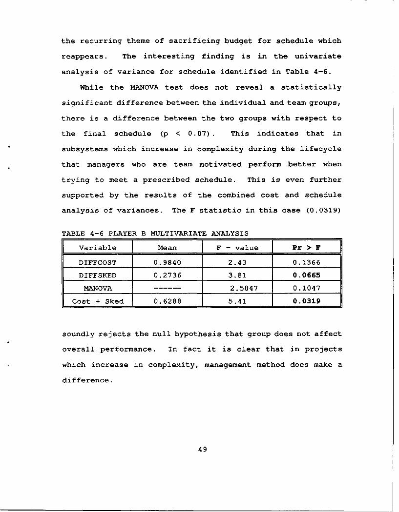
the recurring theme of sacrificing budget for schedule which

reappears. The interesting finding is in the univariate

analysis of variance for schedule identified in Table 4-6.

While the MANOVA test does not reveal a statistically

significant difference between the individual and team groups,

there is a difference between the two groups with respect to

the final schedule (p < 0.07). This indicates that in

subsystems which increase in complexity during the lifecycle

that managers who are team motivated perform better when

trying to meet a prescribed schedule. This is even further

supported by the results of the combined cost and schedule

analysis of variances. The F statistic in this case (0.0319)

TABLE 4-6 PLAYER B MULTIVARIATE ANALYSIS

I Variable Mean F - value Pr > F

DIFFCOST 0.9840 2.43 0.1366

DIFFSKED 0.2736 3.81 0.0665

MANOVA 2.5847 0.1047

Cost + Sked 0.6288 5.41 0.0319

soundly rejects the null hypothesis that group does not affect

overall performance. In fact it is clear that in projects

which increase in complexity, management method does make a

difference.

49

7. Repeated Measures Analysis

A repeated measures analysis was conducted for

evaluating staffing level decisions. The staffing level

decision data for the "AI" versus "AT" and the "BI" versus

"BT" comparisons are included in Appendix Q. The related SAS

control files are included in Appendix R. A graph of the

staffing level decisions is included earlier in this chapter.

The following results of the SAS analysis report the findings

identified in the Wilks' Lambda statistics.

The first test evaluated the hypothesis of no TIME

effect on the staffing level decisions. The "BI" versus "BT"

comparison is significant (F(7,12) = 4.74, p < 0.011 while the

"AI" versus "AT" comparison is not significant {F(7,12) =

1.41, p < 0.29}. Thus, there is a time effect for staffing

level decisions for projects which significantly increase in

complexity, but not in size, over the life of the project.

The second test evaluated the hypothesis for between

subjects effects. The "BI" versus "BT" comparison is

significant (mean: 13.2; F value: 9.04; p < 0.01} while the

"AI" versus "AT" comparison is not significant {mean: 9.6; F

value: 1.75; p < .20}. It appears that the staffing level

decisions for project "B" were affected by the specific group

assigned while the staffing level decisions for project "A"

were independent of group assigned.

50

The third test evaluated the hypothesis of no

TIME*GROUP effect. None of the comparisons were significant,

which indicated that group behavior did not differ over time.

The results of the repeated measures tests show that

the behavior of the subjects who managed subsystems in which

complexity roughly doubled over the life of the project

differs depending on their method of motivation. Combined

with the findings above, these results suggest that subsystem

managers who are managing projects which significantly

increase in complexity during the lifecycle behave differently

when team motivated, and perform better.

C. SUMMARY

The multi-project experiment was conducted using a

properly randomized sample population. This was verified by

statistical analysis of the grade distribution of the assigned

subject groups. Subject data which fell outside the range of

normality were eliminated as noise which could contaminate

statistical analysis. Figure 4-7 summarizes the specific

findings of the thesis. The following items summarize these

three findings:

" The performance of subsystem managers in a multi-projectsoftware development environment is significantly betterwhen the managers are provided with a "Team" incentivestructure versus an "Individually"-competitive structure.

" The performance of subsystem managers in a subsystem whichroughly doubles in complexity during the project lifecycleis significantly better when provided with a "Team"-incentive structure. These managers performed

51

significantly better when trying to meet a prescribedschedule.

* The performance of subsystem managers in a subsystem whichroughly doubles in size during the project lifecycle isnot significantly different for either incentivestructure.

PERFORMANCE ENVIRONMENT

T > I Multi-project systems,overall.

T > I Subsystems which doublein complexity.

T = I Subsystems which doublein size.

Figure 4-7 Multi-Project Experiment Summary

The measure of performance in each case is the ability of

managers to meet final cost and schedule in a dynamic software

development environment. In all cases, the deviation from

final schedule was less than the deviation from final cost.

Further, the staffing level decisions reveal that the work

force ceiling imposed allowed completion of the experiment

with excess staff resources. The finding associated with

these facts indicates that if the staff resources are

available, that managers will sacrifice final cost in order to

meet the final schedule.

The trends implied by the staffing level decisions

indicate that "Team"-motivated managers use the available

resources more efficiently. The "Individually"-motivated

52

managers tended to use fewer resources early and to increase

rapidly the staff size at the end of the project.

53

V. CONCLUSIONS

A. FINDINGS AND IMPLICATIONS

The objective of the thesis has been two-fold: to conduct

an experiment on multi-project management motivation and to

produce a template thesis which serves as a basis for future

experimental studies.

In a time of decreasing budgets and increasing oversight,

the thesis creates and tests by experimentation the affects of

"Team" versus "Individual" motivation on managers who are

operating with limited staff resources. To date, software

project cost estimation tools have proven effective for

predicting a project's cost and schedule in a set environment.

These cost estimation tools are company specific and must be

evaluated over time. As recent Congressional reports have

indicated, industry in general and the Department of Defense

specifically continues to have disastrous problems with cost

and schedule overruns. These overruns are costing millions of

dollars and damage the confidence and credibility of software

cost estimation.

The problem stems from the fact that there are sufficient

software development and estimation products available, yet a

correct management process has not been identified. This is

primarily due to the extreme dynamics that surround software

54

development. It is therefore necessary to model this

environment and test management theory.

The thesis was designed to investigate the affects of

incentive structure on management performance, by using the

System Dynamics Model gaming interface. Managers were

provided with either a competitive or cooperative incentive

structure for two project subsystems with limited staff

resources. The experimental results confirm that project

management teams perform better when trying to deliver a

software project on time and on budget, while operating under

restricted resources, and when provided with a cooperative

incentive structure. These findings suggest that in dynamic

environments with limited resources, team-motivated management

pairs are more successful in delivering software projects on

time and on budget.

B. FURTHER RESEARCH

There are four significant areas of potential research

using the SDM gaming interface to investigate managerial

heuristics in software development.

The first area involves a replication of this multi-

project experiment and delaying the start of the second

project. Preliminary simulations conducted during the design

formulation for this thesis follow the indications specified

in previous research that such a dynamic environment might

affect the quality of management decisions. The simulations

55

conducted during design indicated that final effort and cost

reacted most strongly with a 100 day delay in the start of the

second subset.

The second area involves combining this multi-project

experiment with a single project environment to reveal if the

pressures associated with managing more than one project at a

time has an affect on the quality of project management.

The third area involves a replication of this multi-

project experiment with significant increased stress on the

managers by causing high personnel turnover. This further

examines the crisis-management tendencies of managers.

The final area involves an experiment using a new gaming

interface under development which would allow the manager to

manipulate several management decisions in addition to the

staffing levels.

56

APPENDIX A: DYNEX PROGRAM FILE (XPl.DNX)

if #tm<.l thendisplay clear

Important Points to Remember !!!!! 'H

- You are not allowed to discuss this exercise with anyoneother than a lab attendant. Please refrain from discussingthis with other class members until they have completedthe exercise.

- The system will start by showing you the size of the initial coreteam (they developed the requirement specifications). It willthen ask you for your desired staffing level for the remainder ofthe project.

- Next it will run through the first simulation time period (2 months)and provide you with a status report. At the end of each reportingperiod, you will have an option to revise your desired staff level.Make your change to the desired staffing level both on the screenas well as on the documentation sheet provided.

- Keep in mind that if a work force ceiling is imposed on yourproject, the simulation will not allow you to acquire a stafflevel above that ceiling.

A LAB ATTENDANT MUST VERIFY YOUR FINAL RESULTS!

- GOOD LUCK! Press <ENTER> to continue.

dendqchoice Icend 1/1display clear

THE WORK FORCE CEILING FOR THIS PROJECT HAS BEEN SET AT: 7.5

THE SIZE OF THE INITIAL CORE TEAM IS 5.0 People

1) Enter your desired staffing level and press <ENTER>.

* * OR *********

2) Press <ENTER> to keep that same 5.0.

The current staffing level =dendqdq WFNTR1(1)- 0<7.5display clear

57

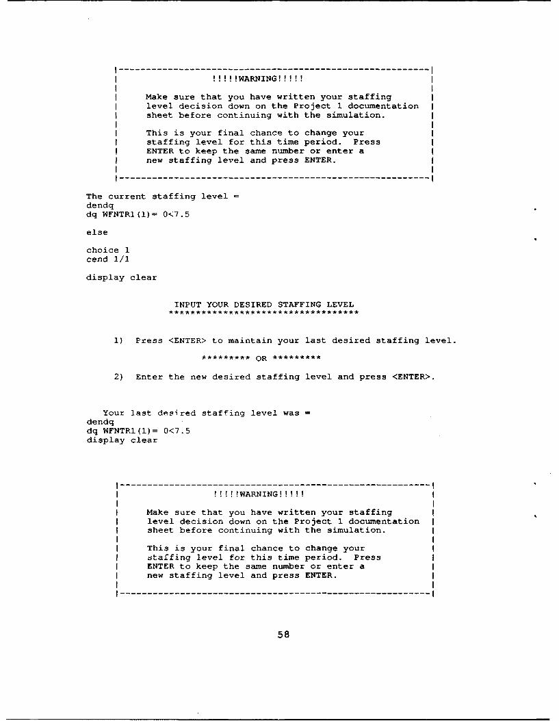
!!!!!WARNING!!!!!

Make sure that you have written your staffinglevel decision down on the Project 1 documentationsheet before continuing with the simulation.

This is your final chance to change yourstaffing level for this time period. PressENTER to keep the same number or enter anew staffing level and press ENTER.

--------------------------------------------------------

The current staffing level =

dendqdq WFNTRl(1)= 0<7.5

else

choice 1cend 1/1

display clear

INPUT YOUR DESIRED STAFFING LEVEL

1) Press <ENTER> to maintain your last desired staffing level.

********* OR *********

2) Enter the new desired staffing level and press <ENTER>.

Your last desired staffing level was =

dendqdq WFNTRI(1)= 0<7.5display clear

--------------------------------------------------------I!!!!!WARNING!!!!!

Make sure that you have written your staffinglevel decision down on the Project 1 documentationsheet before continuing with the simulation.

This is your final chance to change yourstaffing level for this time period. PressENTER to keep the same number or enter anew staffing level and press ENTER.

---------------------------------------------------------

58

The current staffing leveldendqdq WFNTR1(1)= 0<7.5

if #tm<90 thenendenddisplay clear

Press <ENTER> to simulate the next time interval.

dendqchoice 1REPORTt ime--maxtime,FORMAT=" 40-""PROJECT STATUS REPORT";;Format=n20<, 54<, 66<n,PICTURE="Z, ZZ9V"I"ELAPSED TIME -- - - ->",tm,"DayS";;

Format=" 5<""ESTIMATES MADE AT THE START OF THE PROJECT-;FORMAT="8<,52<, 66<",PICTURE="ZZZ,ZZZV""Project Size", IPRJSZ (1) ,"Tasks";FORMAT="8<, 52<, 66<", PICTURE="ZZZ, ZZZV""Project Cost in Man Days",ITOTMD(l),"Man Days";FORMAT="8<, 52<, 66<",PICTURE-"ZZZ, ZZZV""Project Duration",TDEV(1) ,"Days";;Format="5<, 52<, 66<", PICTURE="ZZZ, ZZ9V""PROJECT STATUS at Time = = -= =-----= = =>",tm, "Days";FORMAT=-8<, 52<, 66<", PICTURE="ZZZ, ZZ9V. 99""Updated Estimate of Total Project Size",PJBSZ(1),"Tasks";FORMAT="8<, 52<, 66<", PICTURE-"ZZZ,ZZ9V. 99""% Development (Design & Code) Reported Complete",PDVRC(1),"Percent";FORMAT="8<, 52<, 66<", PICTURE-"ZZZ, ZZ9V. 99""% Testing Reported Complete",PTKTST (1) *l00,ulPercentl;;FORMAT=-8<, 52<, 66<", PICTURE="ZZZ,Z9gV. 99""Updated Estimate of Total Man Days",JBSZMD(l),"Man Days";FORMAT="18<, 52<, 66<", PICTURE-"ZZZ, ZZZV. 99""Total Man Days Expended to date",CUMMD (1),"Man Days";;FORMAT=-8<, 52<, 66<", PICTURE-nZZZ, ZZ9V""Updated Est. of Project Duration (start-end)",SCHCDT(l),"Daysn;;

A FORMAT="8<,52<, 66<",PICTURE-"ZZZ,ZZ9V.9""Current Staff Size",FTEQWF(l),"Fulltime Staff";;FORMAT="5<""PRESS <ENTER> TO RETURN TO MENU"cend 1/1spec md-length=#length+40

59

APPENDIX B: DYNEX PROGRAM FILE (EXP2.DNX)

if #tm<.l thendisplay clear

Important Points to Remember !!!! ! ! !!*********** ***************************

- The system will ttart by showing you the size of the initial coreteam (they developed the requirement specifications). It willthen ask you for you. desired staffing level for the remainder ofthe lifecycle.

- Staffing decisions need to be coordinated with the other subsystemmanaet to ensure that the sum of the two does not exceed thetotal project work force ceiling.

- Next, the simulation will run through the first time period (40 days)and provide you with a status report for your subsystem. At the endof each reporting period, you will have an option to revise yourdesired staff level. Make your changes to the desired staffing level.n the documentation sheet provided as well as on the screen.

- Keep in mind that if a work force ceiling is imposed on yourproject, the simulation will not allow the sum of the staff requests-or the 2 subsystems to be above that ceiling.

A LAB ATTENDANT MUST VERIFY YOUR FINAL RESULTS!

- GOOD LUCK! Press <ENTER> to continue.

dendqchoice 1cend 1/1display clear

THE WORK FORCE CEILING SUM FOR BOTH SUBSYSTEMS HAS BEEN SET AT: 15.0

THE SIZE OF YOUR INITIAL CORE TEAM IS: 5.0 People

FIRST, Deter'ine your desired staff level alone.SECOND, Be prepared to present and defend your subsystem needs to

the other manager.THIRD, When the other manager is ready, have a conference to discuss

your needs.FCIJRTH, You must together:

1. Agree on the desired staff levels for both subsystems.2. Ensure that the sum of both is below the work force ceiling.

FIFTH, Enter the desired staffing level for both subsystems into thedocumentation sheet. (You both do this individually)

SIXTH, Enter the desired staffing level for both subsystems into theComputer. Press <ENTER> to keep the current values, otherwisetype in the new values.

60

Your subsystem current staffing level =dendqdq WFNTR1(1)= 0<15display

Other subsystem current staffing level =dendqdq WFNTRI(2)= 0<#(15-WFNTR1(1))display clear

-----------------------------------------------------I!!!!!WARNING!!!!!

Make sure that you have written the staffinglevel decisions for both subsystems down onyour documentation sheet before continuingwith the simulation.

This is your final chance to check and correctstaffing levels for this time period. PressENTER to keep the same numbers or entercorrected staffing levels and press ENTER.

-----------------------------------------------------I

Your subsystem selected staffing level =dendqdq WFNTR1(1)= 0<15displayOther subsystem selected staffing level =dendqdq WFNTRI(2)= 0<#(15-WFNTR1(1))

else

choice 1cend 1/1display clear

INPUT YOUR DESIRED STAFFING LEVEL

SIXTH, Enter the desired staffing level for both subsystems into theComputer. Press <ENTER> to keep the current values, otherwisetype in the new values.

Your subsystem current staffing level =dendqdq WFNTR1(1)- 0<15display

Other subsystem current staffing level =dendqdq WFNTR1(2)= 0<#(15-WFNTR1(1))display clear

61

!!!!!WARNING!!!!!

Make sure that you have written the staffinglevel decisions for both subsystems down onyour documentation sheet before continuingwith the simulation

This is your final chance to check and correctstaffing levels for this time period. PressENTER to keep the same numbers or entercorrected levels and press ENTER.

----------------------------------------------------- I

Your subsystem selected staffing level =dendqdq WFNTR1(1)= 0<15displayOther subsystem selected staffing level =dendqdq WFNTRI(2)= 0<#(15-WFNTRI(1))

if #tm<90 thenendenddisplay clear

Press <ENTER> to simulate the next time interval.

dendqchoice 1

62

REPORTt ime--maxt ime,FORMAT="4 0-""SUBSYSTEM STATUS REPORT",,Format="20<, 54<, 66<", PICTURE="Z, ZZ9V""ELAPSED TIME == = ==>",tm, "Days";;Fo rmat=" 5<""ESTIMATES MADE AT THE START OF THE PROJECT-;FORMAT--8<,52<, 66<",PICTURE="ZZZ,ZZZV""Subsystem Size", IPRJSZ (1) ,"Tasks";FORMAT="8<, 52<, 66<", PICTURE="ZZZ, ZZZV""Subsystem Cost in Man Days",ITOTMD(1),"Man Days";FORMAT="8<, 52<, 66<", PICTURE="ZZZ, ZZZV""Subsystem Duration",TDEV(1) ,"Days";;Format="5<, 52<, 66<", PICTURE="ZZZ, ZZ9V""SUBSYSTEM STATUS at Time-- = = = = = = == = >",tm, "Days";FORMAT="8<, 52<, 66<", PICTURE="ZZZ, ZZ9V. 99""Updated Estimate of Total Subsystem Size",PJBSZ(l),"Tasks";FORMAT="8<, 52<, 66<", PICTURE="ZZZ, ZZ9V. 99""% Development (Design & Code) Reported Completen,PDVRC(1),"Percent";FORMAT=-8<,52<,66<"1,PICTURE="ZZZ,ZZ9V.99"11% Testing Reported Complete",PTKTST(1) *100, "Percent";;FORMAT="8<, 52<, 66<", PICTURE="ZZZ, ZZ9V. 99""Updated Estimate of Subsystem Man Days",JBSZMD(1),"Man Days";FORMAT="8<, 52<, 66<",PICTURE="ZZZ, ZZZV. 99""Total Man Days Expended to date",CUMMD(l),"Man Days";;FORMAT=-8<, 52<, 66<",PICTURE="ZZZ, ZZ9V""Updated Est. of Subsystem Duration (start-end)n,SCHCDT(1),"Days";;FORMAT="8<, 52<, 66<", PICTURE="ZZZ, ZZ9V. 9""Current Staff Size",FTEQWF(1) ,"Fulltime Staff";;FORMAT="5<""PRESS <ENTER> TO RETURN TO MENU"cend 1~/1spec md-length=#length+40

63

APPENDIX C: SAMPLE OUTPUT REPORT SCREEN

SUBSYSTEM STATUS REPORT

ELAPSED TIME =========> 400 Days

ESTIMATES MADE AT THE START OF THE PROJECTSubsystem Size 396 TasksSubsystem Cost in Man Days 1,111 Man DaysSubsystem Duration 320 Days

SUBSYSTEM STATUS at Time => 400 DaysUpdated Estimate of Total Subsystem Size 610.02 Tasks% Development (Design & Code) Reported Complete 100.00 Percent% Testing Reported Complete 100.00 Percent

Updated Estimate of Subsystem Man Days 1,714.93 Man DaysTotal Man Days Expended to date 1,714.76 Man Days

Updated Est. of Subsystem Duration (start-end) 290 Days

Current Staff Size 0.1 Fulltime Staff

PRESS <ENTER> TO RETURN TO MENU

64

APPENDIX D: BATCH CONTROL FILE (DUOIY .BAT)

echo offCLSmnit 1GRAPHICSbat IN /p /asmit EXPi -go -- pr - -Is -no -pim 6 -bw

-top dynex EXPi -in EXPI.STT -ac -is -pin 6 -bwsmit EXPi -gmn - -no -pin 6 -bwrep EXP I -out f INTERVAL. OrT -t -bw >KUJLrep EXPi -bw >NULinfoofb ICall -topIExitgoto -top%A

-topi %A- Icolor \IFramCISbegtype

\ID 1 \IF VIEW PROJECT STATUS REPORT

\ID 2 \IF PROCEED TO SIMULATE NEXT TIME PERIODH

Choose an option: (DO NOT HIT <ENTER> AFTER SELECTIONHH)and

-iatkeyl inkey %O 1 if %O # - 1 type %0;if %0 - key~ib returngoto -%O-i

-2ndkeyi inkey %i I if %I # - 1 type %1;if %I - key~ib returnif %I - keyO2O goto -$%O$iif %I - keyOOd goto -$%O$iif %i - keyOS goto -topiif %1 - keyi4b goto -topigoto -%O%ii

-i-1i **** VIEW PROJECT STATUS REPORTrep EXP1 EXPi -outf DUOIY.OUT -t -ac -is -pin 6 -byINKEY %Obat /p /s goto -topi

-2-1 **** PROCEED WITH NEXT SIMULATIONBAT CLSBAT COLOR \lFBAT BEGTYPE

65

* 1. DETERMINE THE STAFFING LEVEL YOU DESIRE FOR THE ** REST OF THE PROJECT. ** 2. WRITE YOUR DESIRED STAFFING LEVEL ON THE ** DOCUMENTATION SHEET PROVIDED. ** 3. PRESS <ENTER> *

* *

ENDbat /p /a goto -top

-%0~1

-$%O$1-%O%ll beep goto -topl

-on.error-if %R > 82 if %R < 90 type !I Floating Point Error !! Igoto -Calc.Cla beep type Unexpected batch file error %R in line %L !exit

66

APPENDIX Z: BATCH CONTROL FILE (PROJZCT2.BAT)

echo offCLSinit 1GRAPHICSbat IN /p /ssmlt EXP2 -go - -pro - -1 -ns -plm 6 -bw

-top dynex EXP2 -in EXP2.STT -sc -is -plm 6 -bwsmit EXP2 -gin - -no -plm 6 -bwrep EXP2 -outf INTERVAL.OUT -t -bw >NULrep EXP2 -bw >NUL

infoofb 1Call -toplExitgoto -top%A

-topl %A = 1color \IFramcISbegtype

I\IA MAIN M9NU \IF I

\IF ENSURE THAT YOU HAVE VIEWED THE STATUS REPORT\IF FOR THIS TIME PERIOD PRIOR TO SELECTING OPTION #2

\ID 1 \IF VIEW YOUR SUBSYSTEM STATUS REPORT

\1D 2 \IF PROCEED TO SIMULATE NEXT TIME PERIOD

Choose an option: (DO NOT HIT <ENTER> AFTER SELECTION1!!)end

-lstkeyl inkey %0 1 if %0 # - 1 type %0;if %0 - key01b returngoto -%O-1

-2ndkeyl inkey %1 I if %l # - 1 type %1;if %i - koy01b returnif %1 - key02O goto -$%O$if %1 - keyOOd goto -$%O5if %1 - key0OS goto -toplif %1 - key14b goto -top1goto -%O%11

-- 1 **** VIEW PROOECT STATUS REPORT *****************rep EXP2 EXP2 -outf JUNK.OUT -t -Sc -is -plm 6 -bwINKEY %0bat /p /a goto -topi

-2-1 **** PROCEED WITH NEXT SIMULATION ********************BAT CLSBAT COLOR \IFBAT BEGTYPE

67

* FIRST, Determine your desired staff level alone. ** SECOND, Be prepared to present and defend your subsystem needs ** to the other manager. ** THIRD, When the other manager is ready, have a conference to ** discuss your needs. ** FOURTH, You must together: *

* 1. Agree on the desired staff levels for both subsystems. ** 2. Ensure that the sum of both is below the ceiling. *

* FIFTH, Enter the desired staffing level for both subsystems ** into the documentation sheet. (You both do this ** individually) *

* Press <ENTER> for step SIX. *

* ********* ** ****** ************************** ****** ************ ** ****** ** **

ENDbat /p /s goto -top

-%0~1-$%051-%O%ll beep goto -topl

-on.error-if %R > 82 if %R < 90 type 1! Floating Point Error I1 Igoto -Calc.Cls beep type Unexpected batch file error %R in line %L lexit

68

APPENDIX F: INITIAL DATA (INIT.EXZ) SOURE CODE

1* INIT.C - Put init info in file *

A nclude "stdio .h#include "dos. h"#include "ctypeh'#include 's~'

main(argc, argv)int argc;char *argv[j;f

struct info userinfo;char logfile [FILESIZE] * outfile [FILESIZE], name [30],

smc[10I;FILE *fl, *f2, *fopeno;

1* Opening formalities ... *if(argc<2) { 1* NO arguments entered *

printf("\nNeed to know if project 1,2 or 3");exit (0);

/* Get mnit info from screen *cls 0';set cursor (6, 5);printf ("Please enter Your Last Name");set cursor(6,35);scanf("%s", name);set cursor (7, 5) ;printf ("Please enter your smc");set cursor (7, 35) ;scanf("%s", smc);/*printf("%s %s", name, amc) ;*/d4os_getdate(&userinfo.date);

strcpy (logf ile, "");Istrcat (logfile, LOGFILE);strcat (logfile, argv(1]);strcpy(outfile, "");st rcat (out f ile, OUTFILE);strcat (outfile, argv[1]);if( (fl=fopen(logfile, "w") )==NULL)

printf("couldn't open %s for write", logfile);exit (0);

69

if( (f2=fopen(outfile, "lwl) )==NULL)printf("\couldn't open %s for write", outfile);exit (0);

fprintf(fl, "\n%s %s"l, name, smc);fprintf(f2, "\n%s %s"l, name, smc);fprintf(fl, "\n%d-%d-%d", userinfo.date.month,

userinfo .date. day, \userinfo date. year);

fprintf(f2, "\n%d-%d-%d", userinfo.date.month,userinfo date. day, \

userinfo. date. year);fclose(fl);fclose (f2);

70

APPENDIX G: DATA STRIPPING (INFOOIB.mX) SOURCE CODE

/* INFOCFB.C - Read infile containing data and put it inout file.

Reads 14 lines and prints out 12 values.*/

#include "stdio.h"#include "dos.h#include "ctype .h"#include "eh

main(argc, argv)int argc;char *arg-v[1;

struct info userinfo;char outfile[FILESIZE], name[30], smc[1Q], tmp[30];char dat[12];FILE *fj, *fo, *fopen();int

1* Opening formalities ... *if(argc<2) { /* NO arguments entered *

printfQ'\nNeed to know if project 1,2 or 311);exit (0);

strcpy(outfile, ")

strcat (outfile, OUTFILE);strcat (outfile, arg-v[11);if( (fi=fopen(INFILE, "r") )==NULL){

printf("\couldn't open %s for read", INFILE);exit (0);

if( (fo=fopen(outfile, "a") )==NULL){printf("\couldn't open %s for write", outfile);exit (0);

/* Read line 1: Current ... Elapsed time *for (i0O; i<6; i++){

fscanf(fi, "1%s", tmp);/*printf("1%s", tmp) ;*/

fscanf(fi, "%s", dat);1* Write line 1 */fprintf(fo, "\n%s ",dat);

71

/* Read line 2: Initial ..... Project *for (i0O; i<9; i++) I

fscanf(fi, "%s", tmp);

}*rnf"s" m)*

/* Read line 3: Project Size ... Tasks*/for (i0O; i<2; i++)f

fscanf(fi, "1%s", tmp);/* printf("%s", tmp);*/

}saff," ' a)fscanf(fi, "%s",, dt);

1* Write line 3 */fprintf(fo, " %s ",dat);

/* Read line 4: Project Duration.... .Days *for (i=O; i<2; i++)(

fscanf(fi, "%s", tmp);/* printf("%s", tmp);*I

}saff," ' a)fscanf(fi, "%W", dt);

1* Write line 4 *1fprintf(fo, "1 %s "1,dat);

/* Read line 5: Reported... .Days *for (i0O; i<12; i++)

fscanf(fi, 11%s", tmp);/* printf("%s", tmp);*/

1* Read line 6: %de.... .Percent *for (i=O; i<4; i++)f

fscanf(fi, "1%s", tmp);1* printf("%s", tmp);*/

fsaff,"%" a)fscanf(fi, "%W", dt);

1* Write line 6 *!fprintf(fo, " %s ",dat);

/* Read line 7: %testing. .... Percent *for (i0O; i<4; i++)

fscanf(fi, "1%s", tmp);-1* printf("%s", tmp);*I

fsaff,"%" a)fscanf(fi, "%W", dt);

/* Write line 7 */fprintf(fo, "%s ",dat);

72

/* Read line 8: Perceived. .Size. .Tasks *for (i=0; i<7; i++)

fscanf (fi, "f%s", tmp);/* printf ("%s", tmp);*

f scanf (f i, %s ', dat) ;fscanf (fi, "%s", tmp) ;/* Write line 8 *1fprintf(fo, " %s ",dat);

/* Read line 9: Perceived. .Cost. .Man Days *for (i=0; i<7; i++l

fscanf(fi, "%s", tmp);1* printf ("%s"v, tmp);*

fscanf(fi, "%s", dat);fscanf(fi, "1%s %s", tmp, tmp);/* Write line 9 */fprintf(fo, " %s ",dat);

1* Read line 10: Total Number... .Staff *for (i=0; i<6; i++)f

fscanf(fi, "%s", tmp);/* printf("%s", tmp);*/

fscanf(fi, "%s", dat);fscanf(fi, "%s %s", tmp, tmp);1* Write line 10 */fprintf (f o, 11 %s ., dat);

/* Read line 11: New Est of... .Days *for (i=0; i<6; i++)

fscanf (fi, "%s", tmp);/* printf ("%s" , tmp);*

fscanf(fi, "1%s", dat);fscanf(fi, "1%s 11, tmp);1* Write line 11 */

* fprintf(fo, "1 %s ". dat);-

/* Read line 12: Maximum Tolerable... .Days ** for (i=0; i<4; i++) {

fscanf(fi, "%s't, tmp);/* printf("%s", tmp);*/

f cn i r1 s dfscanf(fi, "%s", dt);

1* Write line 12 *fprintf(fo, "1 %s ",dat);

73

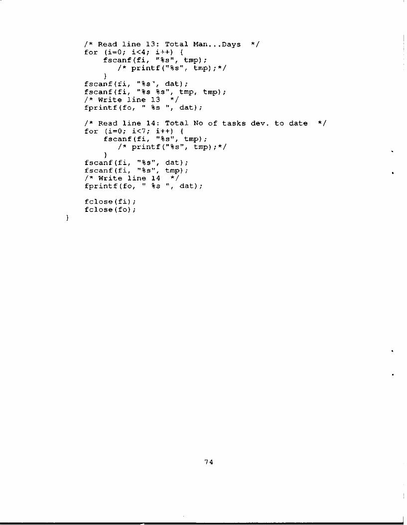
1* Read line 13: Total Man... .Days *for (i=O; i<4; i++){

f scanf (f i, " %s ", tmp);1* printf ("%s", tmp);*

f scanf (f i, " %s ", dat);fscanf(fi, "%s %s", tmp, tmp);/* Write line 13 */fprintf (fo, " %s ", dat);

/* Read line 14: Total No of tasks dev. to date *for (i=O; i<7; i++)

fscanf (fi, "%s", tmp);1*print f(" % s", tmp);*

fscanf(fi, "%s", dat);fscanf(fi, "%s", tmp);/* Write line 14 *fprintf(fo, " %s ",dat);

fclose (fi);fclose (fo);

74

APPENDIX H: MULTI-PROJECT EXPERIMENT COMPUTER SCREENS

Please enter Your Last Name HARDEBECKPlease enter your smc 2293

Important Points to Remember !!!!!!!!

- The system will start by showing you the size of the initial coreteam (they developed the requirement specifications). It willthen ask you for your desired staffing level for the remainder ofthe lifecycle.

- Staffing decisions need to be coordinated with the other subsystemmanager to ensure that the sum of the two does not exceed thetotal project work force ceiling.

- Next, the simulation will run through the first time period (40 days)and provide you with a status report for your subsystem. At the endof each reporting period, you will have an option to revise yourdesired staff level. Make your changes to the desired staffing levelon the documentation sheet provided as well as on the screen.

- Keep in mind that if a work force ceiling is imposed on yourproject, the simulation will not allow the sum of the staff requestsfor the 2 subsystems to be above that ceiling.

A LAB ATTENDANT MUST VERIFY YOUR FINAL RESULTS!

- GOOD LUCK! Press <ENTER> to continue.

75

THE WORK FORCE CEILING SUM FOR BOTH SUBSYSTEMS HAS BEEN SET AT: 15.0THE SIZE OF YOUR INITIAL CORE TEAM IS: 5.0 People

FIRST, Determine your desired staff level alone.SECOND, Be prepared to present and defend your subsystem needs to

the other manager.THIRD, When the other manager is ready, have a conference to discuss

your needs.FOURTH, You must together:

1. Agree on the desired staff levels for both subsystems.2. Ensure that the sum of both is below the work force ceiling.

FIFTH, Enter the desired staffing level for both subsystems into thedocumentation sheet. (You both do this individually)

SIXTH, Enter the desired staffing level for both subsystems into theComputer. Press <ENTER> to keep the current values, otherwisetype in the new values.

Your subsystem current staffing level =5.

THE SIZE OF YOUR INITIAL CORE TEAM IS: 5.0 People

FIRST, Determine your desired staff level alone.SECOND, Be prepared to present and defend your subsystem needs to

the other manager.THIRD, When the other manager is ready, have a conference to discuss

your needs.FOURTH, You must together:

1. Agree on the desired staff levels for both subsystems.2. Ensure that the sum of both is below the work force ceiling.

FIFTH, Enter the desired staffing level for both subsystems into thedocumentation sheet. (You both do this individually)

SIXTH, Enter the desired staffing level for both subsystems into theComputer. Press <ENTER> to keep the current values, otherwisetype in the new values.

Your subsystem current staffing level =5.

Other subsystem current staffing level =5.

76

!!!!!WARNING!!!!!

Make sure that you have written the staffinglevel decisions for both subsystems down onyour documentation sheet before continuingwith the simulation.

This is your final chance to check and correctstaffing levels for this time period. PressENTER to keep the same numbeLs or entercorrected staffing levels and press ENTER.

I----------------------------------------------------------I

Your subsystem selected staffing level =

5.

----------------------------------------------------- I!!!!!WARNING!!!!!

Make sure that yqu have written the staffinglevel decisions for both subsystems down onyour documentation sheet before continuingwith the simulation.

This is your final chance to check and correctstaffing levels for this time period. PressENTER to keep the same numbers or entercorrected staffing levels and press ENTER.

I----------------------------------------------------------I

Your subsystem selected staffing level =

5.

Other subsystem selected staffing level =5.

77

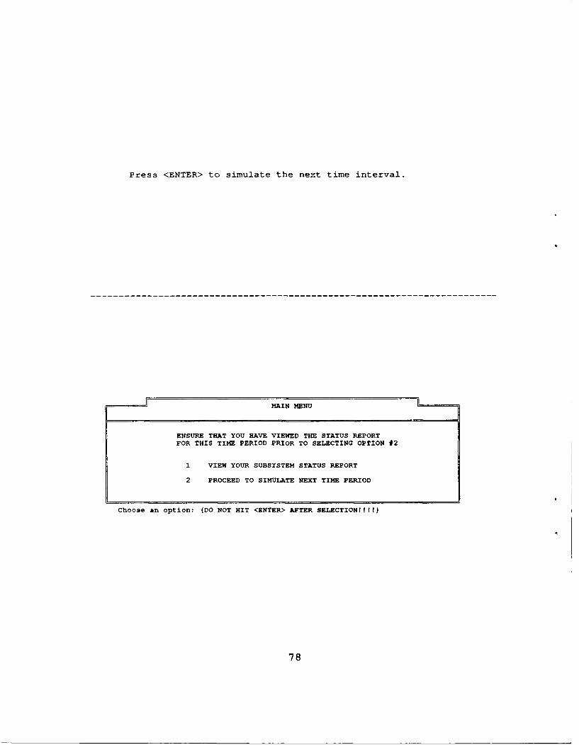
Press <ENTER> to simulate the next time interval.

MAIN MENU

ENSURE THAT YOU HAVE VIEWED THE STATUS REPORTFOR THIS TIME PERIOD PRIOR TO SELECTING OPTION #2

1 VIEW YOUR SUBSYSTEM STATUS REPORT

2 PROCEED TO SIMULATE NEXT TIME PERIOD

Choose an option: (DO NOT HIT <ENTER> AFTER SELECTION! f!)

78

SUBSYSTEM STATUS REPORT

ELAPSED TIME = ========> 40 Days

ESTIMATES MADE AT THE START OF THE PROJECTSubsystem Size 396 TasksSubsystem Cost in Man Days 1,111 Man DaysSubsystem Duration 320 Days

SUBSYSTEM STATUS at Time => 40 DaysUpdated Estimate of Total Subsystem Size 399.38 Tasks% Development (Design & Code) Reported Complete 8.70 Percent% Testing Reported Complete 0.00 Percent

Updated Estimate of Subsystem Man Days 1,111.00 Man DaysTotal Man Days Expended to date 116.92 Man Days

Updated Est. of Subsystem Duration (start-end) 278 DaysCurrent Staff Size 4.0 Fulltime Staff

PRESS <ENTER> TO RETURN TO MENU

** * * ** * * * * * * ** * *****

* FIRST, Determine your desired staff level alone. ** SECOND, Be prepared to present and defend your subsystem needs *

* to the other manager. ** THIRD, When the other manager is ready, have a conference to *

discuss your needs. ** FOURTH, You must together: *

* 1. Agree on the desired staff levels for both subsystems. ** 2. Ensure that the sum of both is below the ceiling. *

* FIFTH, Enter the desired staffing level for both subsystems ** into the documentation sheet. (You both do this ** individually) *

* Press <ENTER> for step SIX. ** *

79

INPUT YOUR DESIRED STAFFING LEVEL

SIXTH, Enter the desired staffing level for both subsystems into theComputer. Press <ENTER> to keep the current values, otherwisetype in the new values.

Your subsystem current staffing level =5.

INPUT YOUR DESIRED STAFFING LEVEL

SIXTH, Enter the desired staffing level for both subsystems into theComputer. Press <ENTER> to keep the current values, otherwisetype in the new values.

Your subsystem current staffing level =5.

Other subsystem current staffing level =5.

80

!!!!!WARNING!!!!!

Make sure that you have written the staffinglevel decisions for both subsystems down onyour documentation sheet before continuingwith the simulation

This is your final chance to check and correctstaffing levels for this time period. PressENTER to keep the same numbers or entercorrected levels and press ENTER.

--------------------------------------------------------I

Your subsystem selected staffing level =

5.

--------------------------------------------------------I!!!!!WARNING!!!!!

Make sure that you have written the staffinglevel decisions for both subsystems down onyour documentation sheet before continuingwith the simulation

This is your final chance to check and correctstaffing levels for this time period. PressENTER to keep the same numbers or entercorrected levels and press ENTER.

--------------------------------------------------------I

Your subsystem selected staffing level =

5.

Other subsystem selected staffing level =

5.

Press <ENTER> to simulate the next time interval.

81

APPENDIX I: "DUMMY" EXPERIMENT DOCUMENTATION

Dummy

YOUR NAME

SMC NO.

INTRODUCTION

The exercise you are about to undeztake is similar in many ways to theflight simulators that pilots use to mimic flying an aircraft from takeoffat point A to landing at point B. Instead of flying an aircraft, though,this simulator mimics the life of a real software project from the startof the design phase until the end of testing. In this simulation, youwill be more than an observer. In fact you will play an important role onthe project: that of the project manager.

Specifically, your role will be to track the project's progress using anumber of status reports that will be produced for you at two-monthintervals (40 working days) during the project. As the project manager,you must then determine the project's staff size based on the knowledgeyou gain from these reports. You can hire additional staff or decreasethe staffing level as you deem necessary to complete the project.

PROJECT

The project that you will manage, happens to have been a real projectconducted in a real organization. The particular organization is on theleading edge in software engineering technology. For the project, youwill be given a project profile containing the following initialinformation:

Estimated Project Size (in No. of tasks)Estimated Duration (in No. of Work Days)Estimated Project Cost (in No. of Man Days)Size of Initial Core Team (in No. of People)

A task is a software module that is approximately 50 lines of code insize. The Core Team is the group of software professionals that developedthe project's requirement specifications. (Remember, you are taking over

at the beginning of the Design Phase).

82

YOUR TASK

Your task is to use the bi-monthly status reports generated by the projectteam at different points in the project to determine a desired staffinglevel for the remainder of the project. Your objective in setting thestaffing level should be to:

(a) complete the project on schedule(b) at the lowest possible cost

YOUR GRADE

Equal weighting will be given to schedule overruns and budget overruns:

(a) Schedule overruns are calculated as follows: Say the initial"Project Duration" is 200 days, and the final completion date is 240days, you will be considered to have overshot the schedule by(240-200)/200 = 20%.

(b) Cost overruns are calculated as follows: Say the initial"Project Cost in Man Days" is 2,000 man days and the final cost atcompletion is 2,500 man days, you will be considered to haveovershot the cost by (2,500-2,000)/2,000 = 25%.

83

SOME IMPORTANT THINGS TO CONSIDER IN MAKING YOUR STAFFING DECISIONS:

1. You will start with a core team that developed your Project'sRequirements. This is to reflect the fact that most projects start outwith a small core team of personnel.

2. As a P .oject manager, you specify the desired staffing level for theremainder of the lifecycle. Of course, the actual staff levels may bedifferent due to things you cannot control such as turnover and lengthyhiring delays.

3. In some cases, a workforce ceiling might be imposed on the project(i.e., because of budgeting considerations). Your staff request mu_ notexceed it.

4. The hiring delay for new employees can take up to 6 weeks. Once newpeople are hired, the assimilation period for a newly hired employee istypically one month long. This is the time needed to train a new employeein the mechanics of the project and bring him/her up to speed. A newemployee (i.e. one that is being trained) is only half as productive as anexperienced employee.

5. The personnel turnover rate is 20% per year.

6. Staff sizes will always be in terms of "Full Time Equivalent"people.

7. At different points in the project you will be given information onthe status of the project. Four key pieces of information for thisstaffing task are:

(a) The "Updated Estimate of Total Project Size" (this can change toreflect the addition of new requirements).

(b) The "Updated Estimate of Total Man Days" (this update can changeto reflect the addition of new requirements and/or changes in theestimate of the team's overall productivity). It is important tonote, that this is an estimate which may or may not be totallyreliable.

(c) The "Total Man Days Expended to date". Subtracting the "TotalMan Days Expended to date" trom "Updated Estimate of Total Man Days"yields the "Remaining Effort in man days."

(d) The "Ut'dated Est. of Project Duration (start-end)". In order todetermine une "Remaining Time", you subtract the "Elapsed Time" frCmthe "Updated Est. of Project Duration (start-end)." It is importantto note, that this is an estimate which may or may not be totallyreliable.

84

8. Let us say that at some point in the project the "Remaining Effort,is 1000 man days, the "Remaining "Time is 100 days and you have 7 fulltime equivalent employees working. You are, thus, in a position where youhave to use your judgement to do one of the following:

I. Stick with the current schedule. If so then you will need astaff size of 1000/100 = 10 full time employees.

2. Stick with your staff size of 7. This means the schedule hasto be pushed back. In this case the model will make the appropriateadjustment to the schedule for you. That is extend it to 1000/7 =

143 man days.

3. Do a bit of both. That is increase the staff size a bit, sayto 8, which will also mean that the schedule will be extended(appropriately by the model) to 1000/8 - 125 days.

85

HOW TO PLAY THE GAME

1. Take some time to practice and get familiar with the system.

(a) Do not start the network. From the C> prompt changedirectories to CD IS4300A.

(b) Type DUMMY for running the dummy project.

(c) The system will show you the size of the initial core team.It will then ask you for your initial desired staffing level.

(d) Determine your desired staffing level for the remainder of thelifecycle.

(e) Ensure that your request does not exceed the workforce

ceiling.

(f) Input your desired staffing level on your documentation sheet.

(g) Enter the staff level number into your PC.

(h) Next the simulation will run through the first simulation timeperiod and show you the "MAIN MENU".

(I) Press 1 to view the status report. DO NOT HIT ENTER AFTERMENU SELECTIONS. Please be sure you understand the report.

(j) Perform steps (d) thru (h), for as many intervals as necessary(by pressing 2), till you are comfortable with the system. Run thedummy project for a minimum of 2 intervals.

(k) After you are finished, hit <ESC> when you are at the "MAINMENU" screen to exit. This is the only time you should hit <ESC>.

(1) Turn your disk and documentation sheet in to the labattendant.

86

DULI4Y

Management's Initial Project Estimates

Initial Estimate of Project Size: 396 TasksInitial Estimate of Project Cost: 1,111 Man DaysInitial Estimate of Project Duration: 320 DaysSize of Initial Core Team: 5 People

A project is considered complete when "% Reported Complete" = 100 for both

development work (i.e., Design and Coding) and testing.

Staffing Level Sought

Please enter your staffing decisions below:

At start of Simulation:

Time elapsed - 40 days:

Time elapsed - 80 days:

Time elapsed - 120 days:

Time elapsed - 160 days:

Time elapsed - 200 days:

Time elapsed - 240 days:

Time elapsed - 280 days:

Time elapsed - 320 days:

Time elapsed - 360 days:

Time elapsed - 400 days:

Time elapsed - 440 days:

Time elapsed - 480 days:

Time elapsed - 520 days:

Time elapsed - 560 days:

Time elapsed - 600 days:

Time elapsed - 640 days:

*** WHEN YOU ARE DONE, CALL FOR A LAB ATTENDANT ***

87