Monte Carlo integration over stepping stone models for spatial genetic inference using approximate Bayesian computation

INFERRING PROCESSES DURING INTRODUCTION AND RANGE EXPANSION

Monte Carlo integration over stepping stonemodels forspatial genetic inference using approximate Bayesiancomputation

STUART J. E. BAIRD,*† and FILIPE SANTOS*†

*Centro de Investigacao em Biodiversidade e Recursos Geneticos (CIBIO ⁄UP), Campus Agrario de Vairao, 4485-661 Vairao,Portugal, †Centre de Biologie et de Gestion des Populations (CBGP), Campus International de Baillarguet CS 30 016, 34988Montferrier ⁄Lez cedex. France

Abstract

Approximate Bayesian computation (ABC) substitutes simulation for analytic models inBayesian inference. Simulating evolutionary scenarios under Kimura’s stepping stone model(KSS) might therefore allow inference over spatial genetic process where analytical resultsare difficult to obtain. ABC first creates a reference set of simulations and would proceed bycomparing summary statistics over KSS simulations to summary statistics from localitiessampled in the field, but: comparison of which localities and stepping stones? Identical step-ping stones can be arranged so two localities fall in the same stepping stone, nearest or diago-nal neighbours, or without contact. None is intrinsically correct, yet some choice must bemade and this affects inference. We explore a Bayesian strategy for mapping field observa-tions onto discrete stepping stones. Wemake Sundial, for projecting field data onto the plane,available. We generalize KSS over regular tilings of the plane. We show Bayesian averagingover the mapping between a continuous field area and discrete stepping stones improves thefit between KSS and isolation by distance expectations. We make Tiler Durden available forcarrying out this Bayesian averaging. We describe a novel parameterization of KSS based onWright’s neighbourhood size, placing an upper bound on the geographic area represented bya stepping stone and make it available as m Vector. We generalize spatial coalescence recur-sions to continuous and discrete space cases and use these to numerically solve for KSS coa-lescence previously examined only using simulation. We thus provide applied and analyticalresources for comparison of stepping stone simulations with field observations.

Keywords: approximate Bayesian computation, geometric probability, Monte Carlo integration,nearest-neighbour stepping stone models

Received 11 December 2009; revision received 24 February 2010, 9 March 2010; accepted 10 March 2010

The need for explicit spatial models of evolutionary pro-cess is now well recognized (see Guillot et al. (2009) forreview). Approximate Bayesian computation (Tavareet al. 1997; Pritchard et al. 1999; Beaumont et al. 2002)allows explicit algorithmic models to be used instead ofexplicit mathematical models for the purposes of Bayes-ian inference. Simulation of complex evolutionary scenar-ios based on the principles of Kimura’s (1953) steppingstone model might therefore be used to make inference

over spatial genetic process where explicit analyticalresults are difficult to obtain. Stepping stone models havea long history in population genetics. They were first pro-posed by Malecot (1949, 1950) but did not gain a largeaudience until the work of Kimura (1953). Kimura’ssteeping stone model has found wide application as atractable approximation to relatedness in structured pop-ulations (Kimura & Weiss 1964; Maruyama 1970, 1971)and clinal changes in allele frequencies (Christiansen1987). Cox & Durrett (2002) provide a brief overview ofmore recent work on Kimura’s lattice and the equivalent,but independently described, probabilist voter model.Stepping stone models seem an attractive choice for

Correspondence: Stuart J. E. Baird, Fax: +351252661780;E-mail: [email protected]

! 2010 Blackwell Publishing Ltd

Molecular Ecology Resources (2010) 10, 873–885 doi: 10.1111/j.1755-0998.2010.02865.x

approximate Bayesian computation (ABC) for pragmaticreasons: their equilibrium properties are well understood(Sawyer 1976; Epperson 2003), allowing verification ofsimulation algorithms, and their simplicity makes themcomputationally efficient. Conversely, we might ask: isABC the best choice for inference over stepping stonemodels? The explicit nature and time reversibility ofstepping stone models makes them, at least in principle,open to exact Bayesian computation. We will return tothis topic in the discussion. For the moment, we suggestthe current absence of such exact computationapproaches may indicate their design is not straightfor-ward, a problem avoided by the relative simplicity ofABC design. This design convenience has a cost: withABC, we trade-off design simplicity against both accu-racy and computational burden, as the first stage of ABCinference is to create a (very) large reference set of simu-lations. The computational efficiency of the steppingstone algorithm reduces this burden. Given this referenceset, ABC could proceed by comparing summary statisticsover stepping stone simulation outcomes to summarystatistics from localities sampled in the field. For a spreadof field sampling locations the question arises: whichfield localities should be compared with which steppingstones? Identical stepping stones can be arranged such

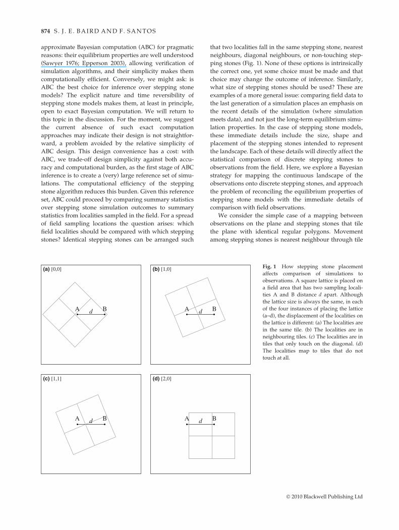
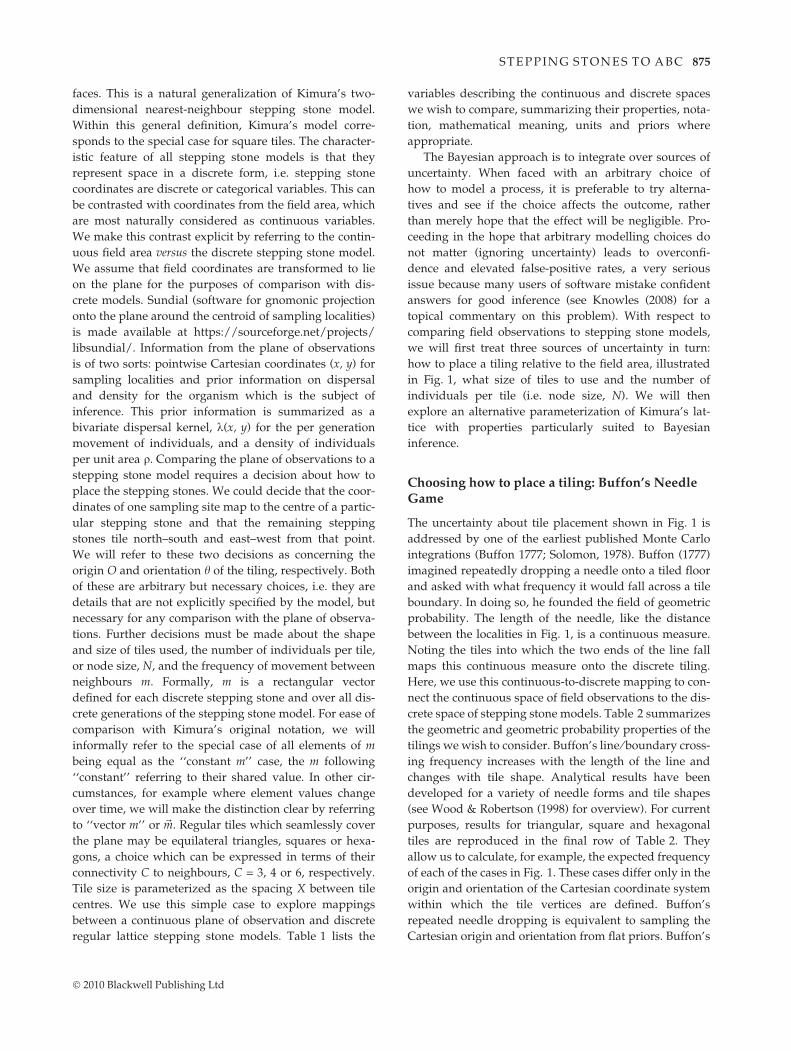
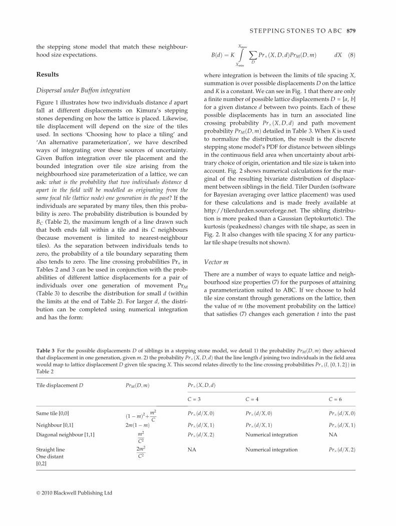
that two localities fall in the same stepping stone, nearestneighbours, diagonal neighbours, or non-touching step-ping stones (Fig. 1). None of these options is intrinsicallythe correct one, yet some choice must be made and thatchoice may change the outcome of inference. Similarly,what size of stepping stones should be used? These areexamples of a more general issue: comparing field data tothe last generation of a simulation places an emphasis onthe recent details of the simulation (where simulationmeets data), and not just the long-term equilibrium simu-lation properties. In the case of stepping stone models,these immediate details include the size, shape andplacement of the stepping stones intended to representthe landscape. Each of these details will directly affect thestatistical comparison of discrete stepping stones toobservations from the field. Here, we explore a Bayesianstrategy for mapping the continuous landscape of theobservations onto discrete stepping stones, and approachthe problem of reconciling the equilibrium properties ofstepping stone models with the immediate details ofcomparison with field observations.

We consider the simple case of a mapping betweenobservations on the plane and stepping stones that tilethe plane with identical regular polygons. Movementamong stepping stones is nearest neighbour through tile

A Bd

A Bd

A Bd

A Bd

(a) [0,0] (b) [1,0]

(d) [2,0](c) [1,1]

Fig. 1 How stepping stone placementaffects comparison of simulations toobservations. A square lattice is placed ona field area that has two sampling locali-ties A and B distance d apart. Althoughthe lattice size is always the same, in eachof the four instances of placing the lattice(a–d), the displacement of the localities onthe lattice is different: (a) The localities arein the same tile. (b) The localities are inneighbouring tiles. (c) The localities are intiles that only touch on the diagonal. (d)The localities map to tiles that do nottouch at all.

! 2010 Blackwell Publishing Ltd

874 S . J . E . BAIRD AND F. SANTOS

faces. This is a natural generalization of Kimura’s two-dimensional nearest-neighbour stepping stone model.Within this general definition, Kimura’s model corre-sponds to the special case for square tiles. The character-istic feature of all stepping stone models is that theyrepresent space in a discrete form, i.e. stepping stonecoordinates are discrete or categorical variables. This canbe contrasted with coordinates from the field area, whichare most naturally considered as continuous variables.We make this contrast explicit by referring to the contin-uous field area versus the discrete stepping stone model.We assume that field coordinates are transformed to lieon the plane for the purposes of comparison with dis-crete models. Sundial (software for gnomonic projectiononto the plane around the centroid of sampling localities)is made available at https://sourceforge.net/projects/libsundial/. Information from the plane of observationsis of two sorts: pointwise Cartesian coordinates (x, y) forsampling localities and prior information on dispersaland density for the organism which is the subject ofinference. This prior information is summarized as abivariate dispersal kernel, k(x, y) for the per generationmovement of individuals, and a density of individualsper unit area q. Comparing the plane of observations to astepping stone model requires a decision about how toplace the stepping stones. We could decide that the coor-dinates of one sampling site map to the centre of a partic-ular stepping stone and that the remaining steppingstones tile north–south and east–west from that point.We will refer to these two decisions as concerning theorigin O and orientation h of the tiling, respectively. Bothof these are arbitrary but necessary choices, i.e. they aredetails that are not explicitly specified by the model, butnecessary for any comparison with the plane of observa-tions. Further decisions must be made about the shapeand size of tiles used, the number of individuals per tile,or node size, N, and the frequency of movement betweenneighbours m. Formally, m is a rectangular vectordefined for each discrete stepping stone and over all dis-crete generations of the stepping stone model. For ease ofcomparison with Kimura’s original notation, we willinformally refer to the special case of all elements of mbeing equal as the ‘‘constant m’’ case, the m following‘‘constant’’ referring to their shared value. In other cir-cumstances, for example where element values changeover time, we will make the distinction clear by referringto ‘‘vector m’’ or ~m. Regular tiles which seamlessly coverthe plane may be equilateral triangles, squares or hexa-gons, a choice which can be expressed in terms of theirconnectivity C to neighbours, C = 3, 4 or 6, respectively.Tile size is parameterized as the spacing X between tilecentres. We use this simple case to explore mappingsbetween a continuous plane of observation and discreteregular lattice stepping stone models. Table 1 lists the

variables describing the continuous and discrete spaceswe wish to compare, summarizing their properties, nota-tion, mathematical meaning, units and priors whereappropriate.

The Bayesian approach is to integrate over sources ofuncertainty. When faced with an arbitrary choice ofhow to model a process, it is preferable to try alterna-tives and see if the choice affects the outcome, ratherthan merely hope that the effect will be negligible. Pro-ceeding in the hope that arbitrary modelling choices donot matter (ignoring uncertainty) leads to overconfi-dence and elevated false-positive rates, a very seriousissue because many users of software mistake confidentanswers for good inference (see Knowles (2008) for atopical commentary on this problem). With respect tocomparing field observations to stepping stone models,we will first treat three sources of uncertainty in turn:how to place a tiling relative to the field area, illustratedin Fig. 1, what size of tiles to use and the number ofindividuals per tile (i.e. node size, N). We will thenexplore an alternative parameterization of Kimura’s lat-tice with properties particularly suited to Bayesianinference.

Choosing how to place a tiling: Buffon’s NeedleGame

The uncertainty about tile placement shown in Fig. 1 isaddressed by one of the earliest published Monte Carlointegrations (Buffon 1777; Solomon, 1978). Buffon (1777)imagined repeatedly dropping a needle onto a tiled floorand asked with what frequency it would fall across a tileboundary. In doing so, he founded the field of geometricprobability. The length of the needle, like the distancebetween the localities in Fig. 1, is a continuous measure.Noting the tiles into which the two ends of the line fallmaps this continuous measure onto the discrete tiling.Here, we use this continuous-to-discrete mapping to con-nect the continuous space of field observations to the dis-crete space of stepping stone models. Table 2 summarizesthe geometric and geometric probability properties of thetilings we wish to consider. Buffon’s line ⁄boundary cross-ing frequency increases with the length of the line andchanges with tile shape. Analytical results have beendeveloped for a variety of needle forms and tile shapes(see Wood & Robertson (1998) for overview). For currentpurposes, results for triangular, square and hexagonaltiles are reproduced in the final row of Table 2. Theyallow us to calculate, for example, the expected frequencyof each of the cases in Fig. 1. These cases differ only in theorigin and orientation of the Cartesian coordinate systemwithin which the tile vertices are defined. Buffon’srepeated needle dropping is equivalent to sampling theCartesian origin and orientation from flat priors. Buffon’s

! 2010 Blackwell Publishing Ltd

STEPPING STONES TO ABC 875

original question allows us to map two localities (one ateither end of the line joining them) to a discrete steppingstone model. More generally, for any number of sampling

localities, it is straightforward to take a Buffon sample ofthe assignments of localities to stepping stones. Here, werepeat Buffon’s original Monte Carlo integration. Now,

Table 1 Variables and notation for (a) data and prior information from a continuous field area (b) classic parameterization of discretestepping stone models and (c) implicit parameters of stepping stone models that must be made explicit for comparison with fieldinformation

Variable Description Nature Units

a) Data and prior information from a continuous field areak x; y! " Parent–offspring

dispersal distributionProbability density function defined on R2 and normalizedby measuring distance in units r.

r2

(x, y) Cartesian coordinates Pointwise locality positions in R2 (the continuous plane) r; r! "d Distance Distance in any direction on the plane i.e. continuous scalar

‡0.r

q Density Individuals per unit area. Continuous ‡ 0. r)2

b) Explicit parameters of a generalized 2D nearest-neighbour stepping stone modelC Connectivity Discrete 2 {3,4,6}, corresponding to triangular, square and

hexagonal tilesnone

N Node size Number of individuals represented at a lattice node.Continuous ‡ 0.

none

m Movement probability Rectangular vector of probability elements definedover all discrete generations and tiles

none

Constantm Rectangular vector with all element values equal to m noneVector m, (~m) Rectangular vector with all element values at generation

t equal to mt

none

D Lattice displacement A tuple of displacements along each lattice axis ordered fromhighest to lowest magnitude

none

c) Implicit stepping stone parameters made explicit by comparison with field dataO Origin The Cartesian coordinates (x, y) where the lattice origin

is placed in the field arear; r! "

h Lattice orientation The orientation with which the lattice is placed relative to theCartesian axes of the field area

none

X Tile spacing Distance d between tile centres r

Table 2 Geometry, and geometric probability, of the generalized two-dimensional stepping stone model. Space is measured in units ofr, the natural measure given an organism’s parent–offspring distribution. Line crossing probabilities Pr# l; f0; 1; 2g! " are taken fromWood & Robertson (1998), with corrections to the final two hexagonal cases

SymbolPropertyTile shape

Tilings

UnitsTriangle Square Hexagon

C Connectivity 3 4 6X Euclidian distance between tile centroids rA Tile area C

4 TanpC

! "X2 r2

A1 Tile area for X = 1 $1.30 1 $0.87 r2

Bf Upper Bound on the length of a line falling within a focal tile######3X

p ######2X

p1##3

p X rBC Upper Bound on the length of a line with ends falling within a focal tile and its C neighbours

2######3X

p #########10X

p2

#######73X

qr

Pr ·(l, i) Line crossing probability: The probability that a line length l X falling at random on the lattice will cross i tileboundaries

Pr ·(l, 0) 1% 2l2

9 % l!4##3

p%l##

3p

p1% l!4%l"

p 1% l2

3 %l!4%

##3

pl

p

Pr ·(l, 1) % 5l2

9 & l!4##3

p%1##

3p

p2l!2%l"

pl2

3 %l!4%

###3l

p

p

Pr ·(l, 2) 4l2

9 % l2##3

pp

l2

p 0Limit of Pr ·(l, i) solution

l £ 1 l £ 1 l ' 12 Xr

! 2010 Blackwell Publishing Ltd

876 S . J . E . BAIRD AND F. SANTOS

however, the object dropped onto the tiled floor is morecomplex than two points joined by a line. It is, instead, allof the field sampling points. Buffon foresaw such general-izations ‘‘But if instead of throwing into the air a round objectsuch as a coin, one threw an object of another shape such as asquare Spanish pistole, or a needle, or a stick, etc., the problemwould demand a little more geometry, although in general itwould always be possible to give its solution by comparison ofspace.’’ (Buffon 1777). In the intervening years, computershave made such calculation straightforward and here wemake Tiler Durden, software for repeatedly dropping setsof sampling localities onto lattices available at http://tilerdurden.sourceforge.net. In this way, Buffon’s MonteCarlo approach can be used to very precisely integrateover the uncertainty attached to two of the parameters ofthe stepping stone model (the origin O and the orienta-tion of the tiling h). Incorporating this uncertainty into theposterior distribution of the approximate Bayesian com-putation avoids both overconfidence and undue influenceof idiosyncratic juxtapositions of simulation and observa-tion.

Choosing a tile size: the geographic scale ofmovement

The classic approach for relating stepping stone modelsto information from the plane of observations is to matchthe prior on the geographic scale of movement of organ-isms with the scale of movement on the lattice. Assumeprior observations about the organism’s movements eachgeneration are summarized by the distribution k. Theseobservations may originally have been recorded withunits of metres or yards; however, the natural distanceunit r is the one that normalizes k, i.e. when all distancesare measured in terms of r the area under k is 1, and itbecomes a probability density function (PDF). On theplane, r2 is the scale of movement per generation. If k is(radially symmetric) bivariate normal, r2 is the marginalvariance in distance moved per generation. If the dis-tance between tiles centres is X and the probability ofmoving between tiles constant m, the variance in distancemoved per generation on the stepping stones is mX2, andthe stepping stone model can be parameterized by equat-ing the scales of movement observed in nature and simu-lated on the lattice

r2 ( mX2

X ( 1####m

p r!1"

Thus, a range of tile size X is consistent with an observedscale of movement r: Simulations can be run with m any-where between 0 and 1, and so tile size has range one rto infinity.

Choosing the number of individuals at a tile node

We will call the number N of individuals at a tile nodethe node size. We wish to relate the number of individualsin the field area to the node size. A simple approach is toimagine dropping the tile (like a quadrat) in the field andcounting the number of individuals N that fall within itsbounds: this is then the node size for that tile. We haveassumed information on numbers of individuals in thefield is summarized in terms of a prior on the density q.Before proceeding further, note that density is a numberper unit area, or per distance2, and as all distances aremost naturally measured in units of r (see ‘Choosing atile size’), the units of density q are r)2. Mapping a uni-form density prior from the field observations to nodesize is simplified by assuming individuals are distrib-uted according to a homogeneous spatial Poisson pro-cess rate q. (Complications arising from boundaries onthe extent over which the process is defined are avoided,without loss of precision, by defining the process on thesurface of a torus). If tiles have area A, then the numberof individuals per tile is then Poisson distributed withexpectation E N) * ( qA. The simplified model we wish toconsider here is that the node size of each tile is identical,and so we will assume the expected number per tile islarge enough that the effects of local heterogeneitybetween tiles can be ignored, letting N $ E N) * ( qA, orin terms of the tile spacing and connectivity fromTable 2,

N ( C4Tan

pC

$ %X2q !2"

(Note that the units of X and q cancel, leaving N, asexpected, a unit-free count). In the case of square tiles(C = 4), the tile spacing X and the tile side are the same,and the node size simplifies to X2q. For constant distanceX between tile centres, triangles pack less densely on theplane than squares, and hexagons more densely (seeTable 2). The terms involving C in (2) account for thischange in packing density.

An alternative parameterization of Kimura’snearest-neighbour stepping stone model in termsof Wright’s neighbourhood size

In section ‘Choosing how to place a tiling’, where wepoint out that no particular lattice placement is intrinsi-cally ‘‘correct’’, Buffon’s needle game provides a satisfy-ing integration over possible placements. In section‘Choosing the number of individuals at a tile node’, noparticular choice of tile spacing X is intrinsically ‘‘cor-rect’’, and once again, inference will change dependingon the choice made. If tile spacing is very large, then all

! 2010 Blackwell Publishing Ltd

STEPPING STONES TO ABC 877

observed localities may fall within the same tile: allobservations will be treated as if coming from a singlepanmictic node at Hardy–Weinberg equilibrium. Alter-natively, if tile spacing is very small, then the nearest twolocalities may be many tiles distant, requiring manygenerations of nearest-neighbour movement for gene-flow to connect them. It is evident that any inference willthen depend on the tile spacing chosen, making conclu-sions about process based on a single arbitrary choice oftile size, for example Currat & Excoffier (2004), overconfi-dent. We have emphasized that such arbitrary choicescan be ameliorated in the Bayesian context by integratingover them. Integration over uncertainty about choice oftile spacing is however less straightforward than for tileplacement because is it not obvious how to construct ameaningful prior. For example, we might consider a flatprior on m, with 0 and 1 excluded; however, the resultingprior on X is not flat, small tile spacing being favoured ina manner unjustified by any reference to prior informa-tion about the study organism. For these reasons, thestandard parameterization (eqn 1) of the movementprobability m with respect to the variance in parent–offspring distance might seem unsatisfactory in thecurrent context, and here we seek an alternative.

We have assumed the prior information about thestudy organism is in terms of density on the plane andparent–offspring variance. These are the parameters ofWright’s (1943) neighbourhood size 4pqr2. This is theinverse of the probability that two individuals sampledfrom a locality had the same ancestor in the previous gen-eration, assuming Gaussian dispersal, and is a factor thatrepeatedly appears in spatial genetic analysis (Bartonet al. 2002). On Kimura’s lattice, the equivalent probabil-ity that two individuals sampled from a locality had thesame ancestor in the previous generation can be decom-posed into two components: (i) The probability that thefocal individuals originated in the same tile in the previ-ous generation and (ii) the probability that they had thesame parent in that tile. The first component dependsonly on the probability of movement m. It requires thatneither individual has moved from their tile of origin orboth moved in the same direction (from C possibilities).The second component depends only on N. Given bothindividuals originated in the same tile, the probability ofhaving the same parent is simply the inverse of the num-ber N of individuals represented at that tile (the nodesize). Equating Wright’s neighbourhood size with itsequivalent on Kimura’s lattice:

1

4pqr2( 1

N1%m! "2& m

C

$ %2& '

!3"

Substituting (2) for the node size N, densities cancelgiving a spatial relationship between the scale of move-

ment in the field, and tile size, connectivity and probabil-ity of movement on the lattice:

X2

4pr2( C

4Tan

pC

$ %& '%1

1%m! "2& m

C

$ %2& '

!4"

In the case of square tiles (C = 4), this simplifies to:

X2

4pr2( 1%m! "2& m

4

$ %2!5"

As with the standard parameterization (1), a range of tilesize X is consistent with an observed scale of movementr. Under the standard parameterization, simulations canbe run for m between 0 and 1, so the bounds on X are1;1) *r. Here, however, for tile size to be positive, there isan upper bound on m of 4

5 ;1517 ;

3537 for the C = 3,4 and 5

cases, respectively. The square tile area can vary frompr2 ⁄ 4 to 4p r2, and the bounds on X are then approxi-mately 0:89; 3:54) *r. In contrast to the standard parame-terization, the lower bound is smaller than r and theupper bound on tile size is finite. Thus, tilings of finer res-olution can be used, and bounded priors on X can be con-structed. For example, Estoup et al. (this issue) note thatX is the maximum distance an individual can move inone generation, and choose a flat prior on X, within itsbounding interval, as a way or representing their uncer-tainty about the capacity of movement of the focal organ-ism. It seems then that the neighbourhood sizeparameterization may be useful for the purposes of ABC,and so we pursue the approach.

Barton & Wilson (1996) extend the notion of Wright’sneighbourhood size over multiple generations into thepast. They express the probability f(d, t) of coalescence atgeneration t for a pair of gene copies observed distance dapart:

f 0; 1! " ( 1

4pqr2

f 0; t! " ( 1

4pqr21

t%Xt%1

s(1

f 0; t% s! "s

!

f d; t! " ( 1

4pqr2e%d2=4t

t%Xt%1

s(1

f d; t% s! "s

0

B@

1

CA

!6"

(When d is zero, the genes may be considered to be sam-pled from the same locality). Given the equivalent proba-bility F D; t! " that two genes lattice displacement D havetheir MRCA on Kimura’s lattice t generations in the past(see appendix A10), we can successively equate neigh-bourhood size and lattice expectations (cf 3) for eachgeneration further into the past

f 0; t q; r2((! "

( F 0; t q;C;X;mj! " !7"

Each generation densities cancel, allowing numericalsolution for parameterizations of the spatial aspects of

! 2010 Blackwell Publishing Ltd

878 S . J . E . BAIRD AND F. SANTOS

the stepping stone model that match these neighbour-hood size expectations.

Results

Dispersal under Buffon integration

Figure 1 illustrates how two individuals distance d apartfall at different displacements on Kimura’s steppingstones depending on how the lattice is placed. Likewise,tile displacement will depend on the size of the tilesused. In sections ‘Choosing how to place a tiling’ and‘An alternative parameterization’, we have describedways of integrating over these sources of uncertainty.Given Buffon integration over tile placement and thebounded integration over tile size arising from theneighbourhood size parameterization of a lattice, we canask: what is the probability that two individuals distance dapart in the field will be modelled as originating from thesame focal tile (lattice node) one generation in the past? If theindividuals are separated by many tiles, then this proba-bility is zero. The probability distribution is bounded byBC (Table 2), the maximum length of a line drawn suchthat both ends fall within a tile and its C neighbours(because movement is limited to nearest-neighbourtiles). As the separation between individuals tends tozero, the probability of a tile boundary separating themalso tends to zero. The line crossing probabilities Pr· inTables 2 and 3 can be used in conjunction with the prob-abilities of different lattice displacements for a pair ofindividuals over one generation of movement PrM(Table 3) to describe the distribution for small d (withinthe limits at the end of Table 2). For larger d, the distri-bution can be completed using numerical integrationand has the form:

B d! " ( KZXmax

Xmin

X

D

Pr# X;D; d! "PrM D;m! " dX !8"

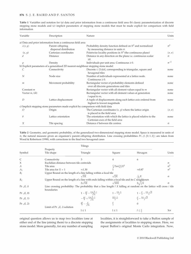
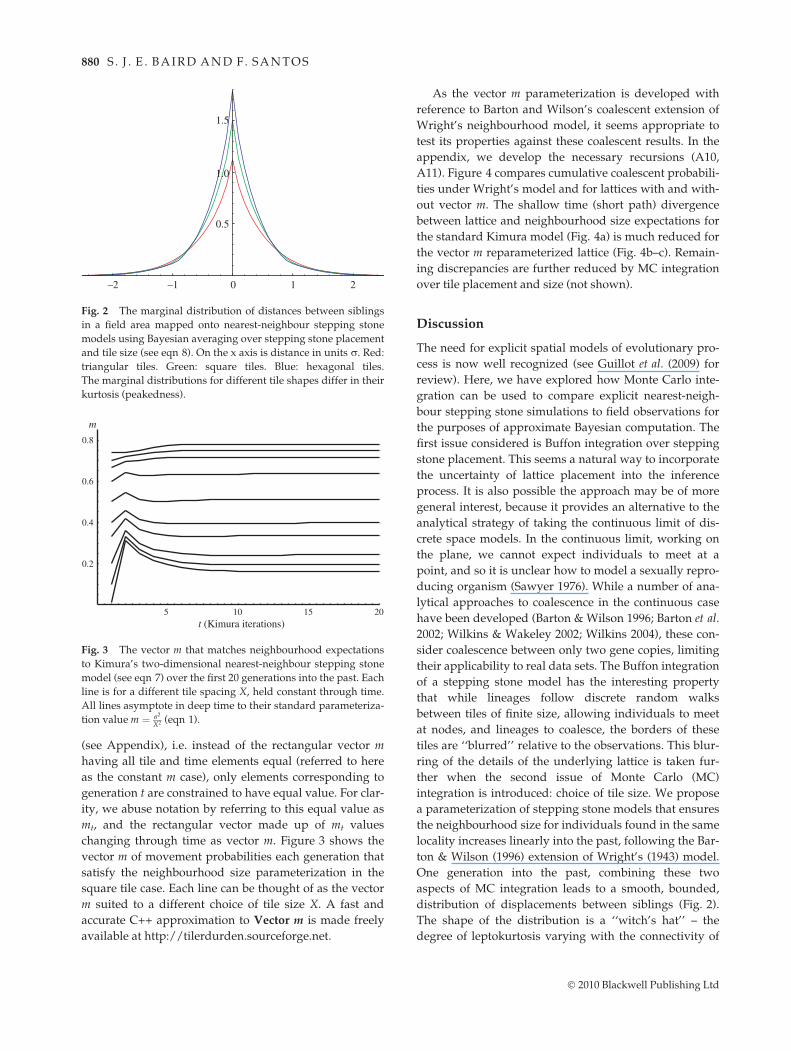
where integration is between the limits of tile spacing X,summation is over possible displacementsD on the latticeand K is a constant. We can see in Fig. 1 that there are onlya finite number of possible lattice displacementsD = [a, b]for a given distance d between two points. Each of thesepossible displacements has in turn an associated linecrossing probability Pr# X;D; d! " and path movementprobability PrM D;m! " detailed in Table 3. When K is usedto normalize the distribution, the result is the discretestepping stone model’s PDF for distance between siblingsin the continuous field area when uncertainty about arbi-trary choice of origin, orientation and tile size is taken intoaccount. Fig. 2 shows numerical calculations for the mar-ginal of the resulting bivariate distribution of displace-ment between siblings in the field. Tiler Durden (softwarefor Bayesian averaging over lattice placement) was usedfor these calculations and is made freely available athttp://tilerdurden.sourceforge.net. The sibling distribu-tion is more peaked than a Gaussian (leptokurtotic). Thekurtosis (peakedness) changes with tile shape, as seen inFig. 2. It also changes with tile spacing X for any particu-lar tile shape (results not shown).

Vector m

There are a number of ways to equate lattice and neigh-bourhood size properties (7) for the purposes of attaininga parameterization suited to ABC. If we choose to holdtile size constant through generations on the lattice, thenthe value of m (the movement probability on the lattice)that satisfies (7) changes each generation t into the past

Table 3 For the possible displacements D of siblings in a stepping stone model, we detail 1) the probability PrM D;m! " they achievedthat displacement in one generation, given m. 2) the probability Pr# X;D; d! " that the line length d joining two individuals in the field areawould map to lattice displacement D given tile spacing X. This second relates directly to the line crossing probabilities Pr# l; f0; 1; 2g! " inTable 2

Tile displacement D PrM D;m! " Pr# X;D; d! "

C = 3 C = 4 C = 6

Same tile [0,0] 1%m! "2&m2

CPr# d=X; 0! " Pr# d=X; 0! " Pr# d=X; 0! "

Neighbour [0,1] 2m 1%m! " Pr# d=X; 1! " Pr# d=X; 1! " Pr# d=X; 1! "

Diagonal neighbour [1,1] m2

C2Pr# d=X; 2! " Numerical integration NA

Straight lineOne distant[0,2]

2m2

C2NA Numerical integration Pr# d=X; 2! "

! 2010 Blackwell Publishing Ltd

STEPPING STONES TO ABC 879

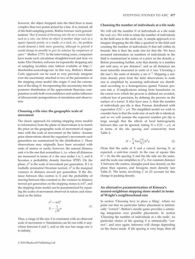
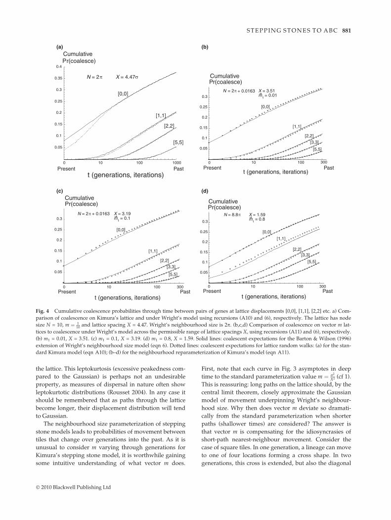
(see Appendix), i.e. instead of the rectangular vector mhaving all tile and time elements equal (referred to hereas the constant m case), only elements corresponding togeneration t are constrained to have equal value. For clar-ity, we abuse notation by referring to this equal value asmt, and the rectangular vector made up of mt valueschanging through time as vector m. Figure 3 shows thevector m of movement probabilities each generation thatsatisfy the neighbourhood size parameterization in thesquare tile case. Each line can be thought of as the vectorm suited to a different choice of tile size X. A fast andaccurate C++ approximation to Vector m is made freelyavailable at http://tilerdurden.sourceforge.net.

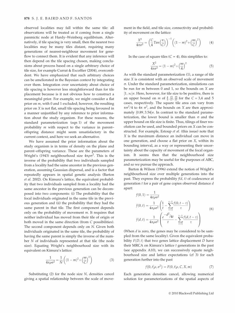
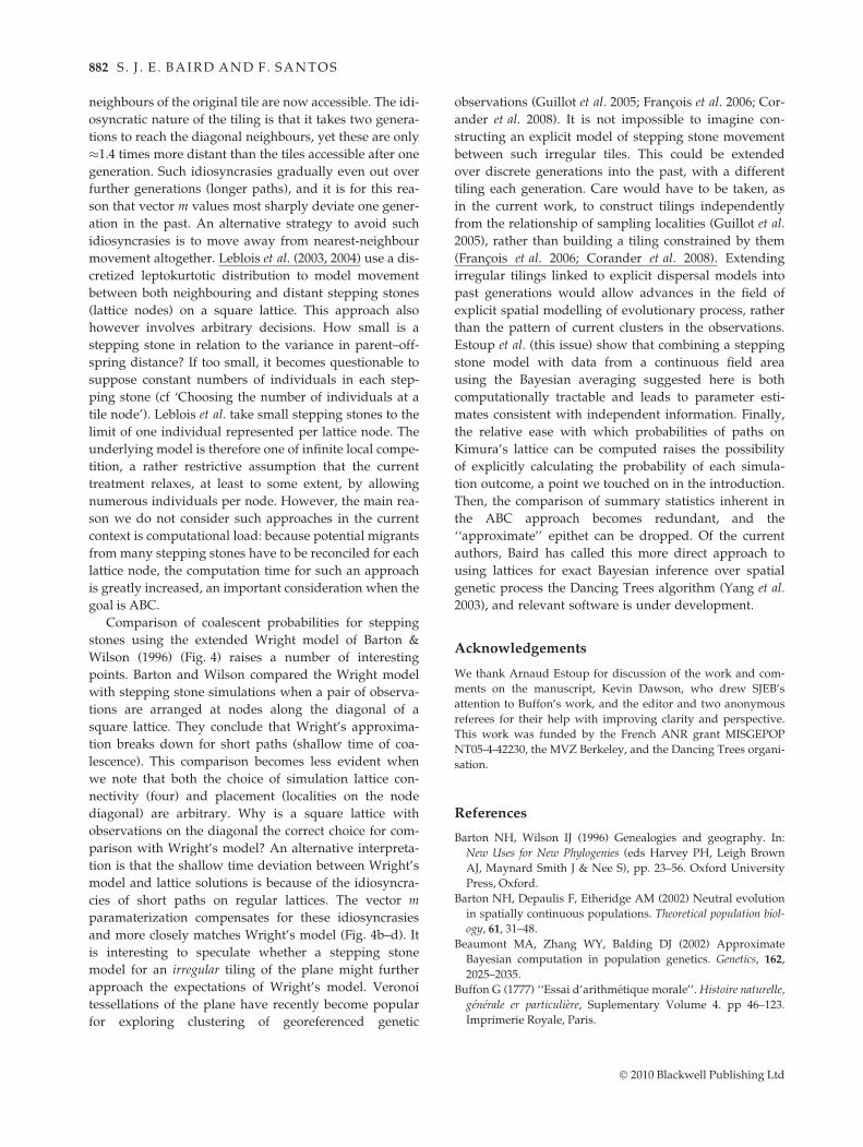
As the vector m parameterization is developed withreference to Barton and Wilson’s coalescent extension ofWright’s neighbourhood model, it seems appropriate totest its properties against these coalescent results. In theappendix, we develop the necessary recursions (A10,A11). Figure 4 compares cumulative coalescent probabili-ties under Wright’s model and for lattices with and with-out vector m. The shallow time (short path) divergencebetween lattice and neighbourhood size expectations forthe standard Kimura model (Fig. 4a) is much reduced forthe vector m reparameterized lattice (Fig. 4b–c). Remain-ing discrepancies are further reduced by MC integrationover tile placement and size (not shown).

Discussion

The need for explicit spatial models of evolutionary pro-cess is now well recognized (see Guillot et al. (2009) forreview). Here, we have explored how Monte Carlo inte-gration can be used to compare explicit nearest-neigh-bour stepping stone simulations to field observations forthe purposes of approximate Bayesian computation. Thefirst issue considered is Buffon integration over steppingstone placement. This seems a natural way to incorporatethe uncertainty of lattice placement into the inferenceprocess. It is also possible the approach may be of moregeneral interest, because it provides an alternative to theanalytical strategy of taking the continuous limit of dis-crete space models. In the continuous limit, working onthe plane, we cannot expect individuals to meet at apoint, and so it is unclear how to model a sexually repro-ducing organism (Sawyer 1976). While a number of ana-lytical approaches to coalescence in the continuous casehave been developed (Barton & Wilson 1996; Barton et al.2002; Wilkins & Wakeley 2002; Wilkins 2004), these con-sider coalescence between only two gene copies, limitingtheir applicability to real data sets. The Buffon integrationof a stepping stone model has the interesting propertythat while lineages follow discrete random walksbetween tiles of finite size, allowing individuals to meetat nodes, and lineages to coalesce, the borders of thesetiles are ‘‘blurred’’ relative to the observations. This blur-ring of the details of the underlying lattice is taken fur-ther when the second issue of Monte Carlo (MC)integration is introduced: choice of tile size. We proposea parameterization of stepping stone models that ensuresthe neighbourhood size for individuals found in the samelocality increases linearly into the past, following the Bar-ton & Wilson (1996) extension of Wright’s (1943) model.One generation into the past, combining these twoaspects of MC integration leads to a smooth, bounded,distribution of displacements between siblings (Fig. 2).The shape of the distribution is a ‘‘witch’s hat’’ – thedegree of leptokurtosis varying with the connectivity of

–2 –1 0 1 2

0.5

1.0

1.5

Fig. 2 The marginal distribution of distances between siblingsin a field area mapped onto nearest-neighbour stepping stonemodels using Bayesian averaging over stepping stone placementand tile size (see eqn 8). On the x axis is distance in units r. Red:triangular tiles. Green: square tiles. Blue: hexagonal tiles.The marginal distributions for different tile shapes differ in theirkurtosis (peakedness).

5 10 15 20

0.2

0.4

0.6

0.8

t (Kimura iterations)

m

Fig. 3 The vector m that matches neighbourhood expectationsto Kimura’s two-dimensional nearest-neighbour stepping stonemodel (see eqn 7) over the first 20 generations into the past. Eachline is for a different tile spacing X, held constant through time.All lines asymptote in deep time to their standard parameteriza-tion valuem ( r2

X2 (eqn 1).

! 2010 Blackwell Publishing Ltd

880 S . J . E . BAIRD AND F. SANTOS

the lattice. This leptokurtosis (excessive peakedness com-pared to the Gaussian) is perhaps not an undesirableproperty, as measures of dispersal in nature often showleptokurtotic distributions (Rousset 2004). In any case itshould be remembered that as paths through the latticebecome longer, their displacement distribution will tendto Gaussian.

The neighbourhood size parameterization of steppingstone models leads to probabilities of movement betweentiles that change over generations into the past. As it isunusual to consider m varying through generations forKimura’s stepping stone model, it is worthwhile gainingsome intuitive understanding of what vector m does.

First, note that each curve in Fig. 3 asymptotes in deeptime to the standard parameterization value m ( r2

X2 (cf 1).This is reassuring: long paths on the lattice should, by thecentral limit theorem, closely approximate the Gaussianmodel of movement underpinning Wright’s neighbour-hood size. Why then does vector m deviate so dramati-cally from the standard parameterization when shorterpaths (shallower times) are considered? The answer isthat vector m is compensating for the idiosyncrasies ofshort-path nearest-neighbour movement. Consider thecase of square tiles. In one generation, a lineage can moveto one of four locations forming a cross shape. In twogenerations, this cross is extended, but also the diagonal

0.05

0.1

0.15

0.2

0.25

0.3

0.35

0.4

t (generations, iterations)

[0,0]

[1,1]

Present Past

[2,2]

[5,5]

0 10 100 1000

N = 2 X = 4.47

CumulativePr(coalesce)

0.05

0.1

0.15

0.2

0.25

0.3

t (generations, iterations)

[0,0]

[1,1]

Present0 100

Past

CumulativePr(coalesce)

[2,2][3,3]

300

[5,5]

10

N = 2 + 0.0163 X = 3.51m

1 = 0.01

0.05

0.1

0.15

0.2

0.25

0.3

[0,0]

[1,1]

Present0 100

Past

CumulativePr(coalesce)

[2,2][3,3]

300

[5,5]

10

N = 2 + 0.0163 X = 3.19m

1 = 0.1

t (generations, iterations)

0.05

0.1

0.15

0.2

0.25

0.3

t (generations, iterations)

[0,0][1,1]

Present0 100

Past

CumulativePr(coalesce)

[2,2][3,3]

300

[5,5]

10

N = 8.8 X = 1.59m

1 = 0.8

(a)

(c)

(b)

(d)

Fig. 4 Cumulative coalescence probabilities through time between pairs of genes at lattice displacements [0,0], [1,1], [2,2] etc. a) Com-parison of coalescence on Kimura’s lattice and under Wright’s model using recursions (A10) and (6), respectively. The lattice has nodesize N = 10, m ( 1

10 and lattice spacing X = 4.47. Wright’s neighbourhood size is 2p. (b,c,d) Comparison of coalescence on vector m lat-tices to coalescence under Wright’s model across the permissible range of lattice spacings X, using recursions (A11) and (6), respectively.(b) m1 = 0.01, X = 3.51. (c) m1 = 0.1, X = 3.19. (d) m1 = 0.8, X = 1.59. Solid lines: coalescent expectations for the Barton & Wilson (1996)extension of Wright’s neighbourhood size model (eqn 6). Dotted lines: coalescent expectations for lattice random walks: (a) for the stan-dard Kimura model (eqn A10); (b–d) for the neighbourhood reparameterization of Kimura’s model (eqn A11).

! 2010 Blackwell Publishing Ltd

STEPPING STONES TO ABC 881

neighbours of the original tile are now accessible. The idi-osyncratic nature of the tiling is that it takes two genera-tions to reach the diagonal neighbours, yet these are only$1.4 times more distant than the tiles accessible after onegeneration. Such idiosyncrasies gradually even out overfurther generations (longer paths), and it is for this rea-son that vector m values most sharply deviate one gener-ation in the past. An alternative strategy to avoid suchidiosyncrasies is to move away from nearest-neighbourmovement altogether. Leblois et al. (2003, 2004) use a dis-cretized leptokurtotic distribution to model movementbetween both neighbouring and distant stepping stones(lattice nodes) on a square lattice. This approach alsohowever involves arbitrary decisions. How small is astepping stone in relation to the variance in parent–off-spring distance? If too small, it becomes questionable tosuppose constant numbers of individuals in each step-ping stone (cf ‘Choosing the number of individuals at atile node’). Leblois et al. take small stepping stones to thelimit of one individual represented per lattice node. Theunderlying model is therefore one of infinite local compe-tition, a rather restrictive assumption that the currenttreatment relaxes, at least to some extent, by allowingnumerous individuals per node. However, the main rea-son we do not consider such approaches in the currentcontext is computational load: because potential migrantsfrom many stepping stones have to be reconciled for eachlattice node, the computation time for such an approachis greatly increased, an important consideration when thegoal is ABC.

Comparison of coalescent probabilities for steppingstones using the extended Wright model of Barton &Wilson (1996) (Fig. 4) raises a number of interestingpoints. Barton and Wilson compared the Wright modelwith stepping stone simulations when a pair of observa-tions are arranged at nodes along the diagonal of asquare lattice. They conclude that Wright’s approxima-tion breaks down for short paths (shallow time of coa-lescence). This comparison becomes less evident whenwe note that both the choice of simulation lattice con-nectivity (four) and placement (localities on the nodediagonal) are arbitrary. Why is a square lattice withobservations on the diagonal the correct choice for com-parison with Wright’s model? An alternative interpreta-tion is that the shallow time deviation between Wright’smodel and lattice solutions is because of the idiosyncra-cies of short paths on regular lattices. The vector mparamaterization compensates for these idiosyncrasiesand more closely matches Wright’s model (Fig. 4b–d). Itis interesting to speculate whether a stepping stonemodel for an irregular tiling of the plane might furtherapproach the expectations of Wright’s model. Veronoitessellations of the plane have recently become popularfor exploring clustering of georeferenced genetic

observations (Guillot et al. 2005; Francois et al. 2006; Cor-ander et al. 2008). It is not impossible to imagine con-structing an explicit model of stepping stone movementbetween such irregular tiles. This could be extendedover discrete generations into the past, with a differenttiling each generation. Care would have to be taken, asin the current work, to construct tilings independentlyfrom the relationship of sampling localities (Guillot et al.2005), rather than building a tiling constrained by them(Francois et al. 2006; Corander et al. 2008). Extendingirregular tilings linked to explicit dispersal models intopast generations would allow advances in the field ofexplicit spatial modelling of evolutionary process, ratherthan the pattern of current clusters in the observations.Estoup et al. (this issue) show that combining a steppingstone model with data from a continuous field areausing the Bayesian averaging suggested here is bothcomputationally tractable and leads to parameter esti-mates consistent with independent information. Finally,the relative ease with which probabilities of paths onKimura’s lattice can be computed raises the possibilityof explicitly calculating the probability of each simula-tion outcome, a point we touched on in the introduction.Then, the comparison of summary statistics inherent inthe ABC approach becomes redundant, and the‘‘approximate’’ epithet can be dropped. Of the currentauthors, Baird has called this more direct approach tousing lattices for exact Bayesian inference over spatialgenetic process the Dancing Trees algorithm (Yang et al.2003), and relevant software is under development.

Acknowledgements

We thank Arnaud Estoup for discussion of the work and com-ments on the manuscript, Kevin Dawson, who drew SJEB’sattention to Buffon’s work, and the editor and two anonymousreferees for their help with improving clarity and perspective.This work was funded by the French ANR grant MISGEPOPNT05-4-42230, the MVZ Berkeley, and the Dancing Trees organi-sation.

References

Barton NH, Wilson IJ (1996) Genealogies and geography. In:New Uses for New Phylogenies (eds Harvey PH, Leigh BrownAJ, Maynard Smith J & Nee S), pp. 23–56. Oxford UniversityPress, Oxford.

Barton NH, Depaulis F, Etheridge AM (2002) Neutral evolutionin spatially continuous populations. Theoretical population biol-ogy, 61, 31–48.

Beaumont MA, Zhang WY, Balding DJ (2002) ApproximateBayesian computation in population genetics. Genetics, 162,2025–2035.

Buffon G (1777) ‘‘Essai d’arithmetique morale’’. Histoire naturelle,generale er particuliere, Suplementary Volume 4. pp 46–123.Imprimerie Royale, Paris.

! 2010 Blackwell Publishing Ltd

882 S . J . E . BAIRD AND F. SANTOS

Christiansen FB (1987) The deviation from linkage equilibriumwith multiple loci varying in a stepping-stone cline. Journal ofGenetics, 40, 45–67.

Corander J, Siren J, Arjas E (2008) Bayesian spatial modeling ofgenetic population structure. Computational Statistics, 23, 111–129.

Cox JT, Durrett R (2002) The stepping stone model: new formu-las expose old myths. Annals of Applied Probability, 12, 1348–1377.

Currat M, Excoffier L (2004) Modern humans did not admix withNeanderthals during their range expansion into Europe. PlosBiology, 2, 2264–2274.

Epperson BK (2003) Geographical Genetics. Princeton UniversityPress, Princeton.

Francois O, Ancelet S, Guillot G (2006) Bayesian clustering usinghidden Markov random fields. Genetics, 174, 805–816.

Guillot G, Mortier F, Estoup A (2005) Geneland: a computerpackage for landscape genetics. Molecular Ecology Notes, 5,712–716.

Guillot G, Leblois R, Coulon A, Frantz AC (2009) Statisticalmethods in spatial genetics.Molecular Ecology, 18, 4734–4756.

Kimura M (1953) Stepping Stone Model of Population. AnnualReport National Institute of Genetics, Japan, 3, 62–63.

Kimura M, Weiss GH (1964) The stepping stone model of popu-lation structure and the decrease of genetic correlation withdistance. Genetics, 49, 561–576.

Knowles LL (2008) Why does a method that fails continue to beused? Evolution, 62, 2713–2717.

Leblois R, Estoup A, Rousset F (2003) Influence of mutationaland sampling factors on the estimation of demographicparameters in a ‘continuous’ population under isolation bydistance.Molecular Biology and Evolution, 20, 491–502.

Leblois R, Estoup A, Rousset F (2004) Influence of spatial andtemporal heterogeneities on the estimation of demographicparameters in a continuous population using individual mi-crosatellite data. Genetics, 166, 1081–1092.

Malecot G (1949) Les processus stochastiques en genetique de popula-tion. Publications de l’Institut de Statistique de Paris I, Volume3, 1–16.

Malecot G (1950) Quelques schemas probabilistes sur la variabilitedes populations. Annales Universitatis Lyon Science, 13, 37–60.

Maruyama T (1970) Analysis of population structure I Onedimensional stepping stone models of finite length. Annals ofHuman Genetics, 34, 201–219.

Maruyama T (1971) Analysis of population structure II Twodimensional stepping stone models of finite length and othergeographically structured populations. Annals of Human Genet-ics, 35, 179–196.

Pritchard JK, Seielstad MT, Perez-Lezaun A, Feldman MW(1999) Population growth of human Y chromosomes: a studyof Y chromosome microsatellites. Molecular Biology and Evolu-tion, 16, 1791–1798.

Rousset F (2004) Genetic Structure and Selection in Subdivided Popu-lations. Princeton University Press, Princeton.

Sawyer S (1976) Results for the stepping stone model for migra-tion in population genetics. Annals of Probability, 4, 699–728.

Solomon (1978) Geometric Probability. Society for Industrial andApplied Mathematics, Philadelphia.

Tavare S, Balding DJ, Griffiths RC, Donnelly P (1997) Inferringcoalescence times from DNA sequence data. Genetics, 145,505–518.

Wilkins JF (2004) A seperation-of-timescales approach to the coa-lescent in a continuous population. Genetics, 168, 2227–2244.

Wilkins JF, Wakeley J (2002) The coalescent in a continuous,finite, linear population. Genetics, 161, 873–888.

Wood GR, Robertson JM (1998) Buffon got it straight. Statisticsand Probability Letters, 37, 415–421.

Wright S (1943) Isolation by distance. Genetics, 28, 114–138.Yang ZH, Stephens D, Dawson KJ et al. (2003) Inferences from

DNA data: population histories, evolutionary processes andforensic match probabilities - Discussion. Journal of the RoyalStatistical Society A, 166, 188–201.

Supporting Information

Additional Supporting Information may be found in theonline version of this article.

Table S1 Transition matrices for displacement on thesquare vector m lattice

Please note: Wiley-Blackwell are not responsible for thecontent or functionality of any supporting informationsupplied by the authors. Any queries (other than missingmaterial) should be directed to the corresponding authorfor the article.

Appendix

The probability of a path length L covering latticedisplacement D on the square lattice with constant m

The probability can be expressed in terms of the permu-tations and combination of events making up a randomwalk with ends at displacement D. For the case of asquare tiling, there are five types of event that we mightlabel { non-movement, north, east, south, west }. In thesimplest case of constant isotropic movement probabilityon the lattice (constant m), the first event type occurs withprobability 1-m, the rest with probability m. Events areexchangeable in the sense that random walks with thesame numbers of each event, no matter their order, willcover the same displacement on the lattice. In the squarecase, if the numbers of events of each type are denotedM0 to M4, respectively, the frequency of walks with eventnumbersM is

P M;m! " (P4

0 MQ40 M!

M1%m0

X4

1M

$ %m!A1"

For a given total number of events L and walk displace-ment D, there are several ways distributing the eventsamong types. This is because pairs of movement events{north, south}, {east, west} cancel in displacement, and soare exchangeable with pairs of nonmovement events. Thewalk displacement D sets the minimum number ofunpaired movement events D1, D2 on each axis, and soalso the maximum number of exchangeable pairs

! 2010 Blackwell Publishing Ltd

STEPPING STONES TO ABC 883

Imax ( )!L% X1 % X2"=2*, where square brackets denotethe integer part. Permuting the exchangeable pairs overthe axes, the frequency of walks length L displacement Dis

G D; L;m! " (XImax

I(0

XImax%I

J(0

P!fL% !D1 &D2 & 2!I & J"";

D1 & I;D2 & J; I; Jg;m" !A2"

Substituting (A1) for P M;m! ", this simplifies to a numeri-cal expression with computation order linear in L, thepath length:

G D; L;m! " ( 1%m! "LC 1& L! "XImax

I(0

m4 1%m! "

& '2I& Dj j H2F1 I % I+; 12 & I % I+; 1&D2; m2

4 1%m! "2

$ %

C 1& I! "C !1& I &D1! "C 1& 2 I & I+! "! "

I+ (L% Dj j

2; Dj j ( D1 &D2 !A3"

This simplification greatly reduces numerical computa-tion over longer paths and arises from substitution of oneof Gauss’ class of hypergeometric functions, H2F1 (g), fora continued fraction expansion. Similar arguments leadto numerical expressions for G for C = 3,6 (not shown).

The probability that two lineages originating at the samelattice point meet after i iterations of the square latticewith vector m

Assume the probability of movement from a steppingstone is equal in all directions, and all values of therectangular vector m are equal for a given generation,or iteration, of the stepping stone algorithm. Then, thelattice has four-way symmetry and we can representthe displacement between two lineages as an orderedtuple along two axes [J,K], J£K. Consider two lineages

that have displacement [0,0] at depth i + 1 on the lat-tice. They could have arrived in this state in one ofseveral ways:

• They had displacement [0,0] at depth i and neithermoved.• They had displacement [0,1] at depth i and onestayed in the same position while the other moved tothat position.

• They had displacement [0,0], [1,1] or [0,2] at depth iand both moved to the same lattice point.

(cf PrM, Table 3). For iteration i of the stepping stonealgorithm denote the value of the rectangular vector mthat is shared over all stepping stones as mi Let Pi = mi

andQi = 1 - mi. Remembering movement is isotropic infour directions

Pr 0; 0) *; i& 1;m! " ( Q2i Pr 0; 0) *; i;m! " & PiQi Pr 0; 1) *; i;m! "

& P2i

!14 Pr!)0; 0*; i;m" & 1

8 Pr!)1; 1*; i;m"& 1

16 Pr!)0; 2*; i;m""

( Pr 0; 0) *; i;m! " Q2i & 1

4

! "

& Pr 0; 1) *; i;m! " PiQi! "& Pr 1; 1) *; i;m! " 1

8P2i

! "

& Pr 0; 2) *; i;m! " 116P

2i

! "!A4"

Thus, the probability of displacement [0,0] at latticedepth i + 1 can be expressed in terms of the probabilitiesof lineages having displacement states [0,0] and [0,1],[1,1], [0,2] in the neighbouring lattice timeslice. Note thatwe already have an expression for the [0,0] case (A4)which can be applied recursively. We can write downsimilar expressions for [0,1], [1,1], [0,2], and so on for allthose states that could in turn give rise to them. Theresulting state transitions have an important property:moving along either axis away from symmetric casessuch as square displacements ([0,0], [1,1], [2,2],…,[J,,J]),off-square displacements ([0,1], [1,2], [2,3],…,[J,,J + 1])and one-dimensional displacements ([0,0], [0,1],[0,2],…,[0,K]), the state transition vectors and probabili-ties begin to repeat. In fact, there are only sixteen states,which we will label a,b,c,…,n,o,p that have unique statetransition descriptions relative to their neighbours. Thesesixteen unique state transitions can be summarized interms of matrices T J;K) *! ") such that:

As a notational convenience, we denote the cumber-some matrix describing the relative positions of neigh-bouring states), so

Pr J;K) *; i& 1;m! " (X

T J;K) *! "Pr }! "; !A6"

where Pr }! " is constructed by replacement of each ele-ment e of ) by Pr e; i;m! ". Eqn A6 is then the matrix

Pr J;K) *; i& 1;m! " (X

T J;K) *! "Pr

0 0 J;K % 2) * 0 00 J % 1;K % 1) * J;K % 1) * J & 1;K % 1) * 0

J % 2;K) * J % 1;K) * J;K) * J & 1;K) * J & 2;K) *0 J % 1;K & 1) * J;K & 1) * J & 1;K & 1) * 00 0 J;K & 2) * 0 0

0

BBBB@

1

CCCCA!A5"

! 2010 Blackwell Publishing Ltd

884 S . J . E . BAIRD AND F. SANTOS

product of Pr }! " and T J;K) *! " (values detailed in TableS 1), and summation is over all the elements of the result.Eqn A6 is a timeslice by timeslice recursive numericalsolution for the probability of a displacement state on asquare lattice with nearest-neighbour movement andvector m (and therefore vectors P,Q) expressing the prob-ability of movement each timeslice. For the case of twolineages originating in the same place at time zero, thebase case of the recursion is

Pr 0; 0) *;m; 0! " ( 1Pr J;K) *;m; 0! " ( 0 otherwise

)!A7"

and the recursion can be made more efficient by notingthat:

Pr J;K) *;m; i! " ( 0 if J & K>2i !A8"

that is because the two lineages start in the same placeand increase their displacement by at most two latticeunits each timeslice, the recursion can be stopped forstates with total displacements exceeding twice the num-ber of elapsed lattice time units.

Pairwise coalescence probabilities for stepping stonemodels

The pairwise coalescence recursion of (Barton & Wilson1996) (eqn 6) involves the convolution of a Gaussian ran-dom walk and generalizes over convolutions of latticerandom walksW D; t! " as:

Fw D; t! " ( 1

2NW D; 2t! " %

Xt%1

s(1

Fw D; t% s! "W 0; 2t! "

!

;

!A9a"

or equivalently

Fw D; t! " ( 1

2NW D; 2t! " %

Xt%1

s(1

W D; t% s! "Fw 0; 2t! "

!

:

!A9b"

Substituting the square lattice constant m convolution(A3) into (A9a), the coalescence probability is:

Fm D; t! " ( 1

2NG D; 2t;m! " %

Xt%1

s(1

Fm D; t% s! "G 0; 2t;m! "

!

:

!A10"

Substituting the square lattice vector m convolution(A6) into (A9a), the coalescent probability is:

F~m D; t! " ( 1

2NPr D; 2t; ~m! " %

Xt%1

s(1

F~m D; t% s! "Pr 0; 2t; ~m! " !

:

!A11"

! 2010 Blackwell Publishing Ltd

STEPPING STONES TO ABC 885