Monroe L. Weber-Shirk S chool of Civil and Environmental Engineering Gravity Water Supply Design.

Monroe L. Weber-Shirk

School of Civil and

Environmental Engineering

Gravity Water Supply DesignGravity Water Supply Design

Population ProjectionPopulation Projection

Example from Agua Para el Pueblo (Honduras)

Count the houses Assume 6 people per house Assume linear growth for design period

N = design period K = growth rate

Example from Agua Para el Pueblo (Honduras)

Count the houses Assume 6 people per house Assume linear growth for design period

N = design period K = growth rate

Población futura ( Pf ) = Pa(1+N*K/100) K = Tasa de crecimiento ( 3.5% ) N = Período de diseño ( 22 años )

( )1future presentP P NK= +

Water DemandWater Demand

Assume a per capita demand (this might be based on a governmental regulation)

Multiply per capita demand by the future population to get design average demand

Multiply average demand by scaling factors to get maximum day demand and maximum hour demand

Assume a per capita demand (this might be based on a governmental regulation)

Multiply per capita demand by the future population to get design average demand

Multiply average demand by scaling factors to get maximum day demand and maximum hour demand

Distribution Storage Tank SizeDistribution Storage Tank Size

Based on 8 hours of storage at average demand

These systems aren’t designed for fire protection

Based on 8 hours of storage at average demand

These systems aren’t designed for fire protection

Design FlowsDesign Flows

Transmission Line Design flow Perhaps based on maximum daily demand or on

maximum hourly demand Distribution system design flows

Take peak hourly flow at the end of the system design life

Divide that flow by the current number of houses to get a flow per house

The flow in each pipe is calculated based on the number of houses downstream

Transmission Line Design flow Perhaps based on maximum daily demand or on

maximum hourly demand Distribution system design flows

Take peak hourly flow at the end of the system design life

Divide that flow by the current number of houses to get a flow per house

The flow in each pipe is calculated based on the number of houses downstream

Pipe DiametersPipe Diameters

How are pipe sizes chosen? Energy Equation An equation for head loss Requirement of minimum pressure in the

system

How are pipe sizes chosen? Energy Equation An equation for head loss Requirement of minimum pressure in the

system

Ltp hhzg

Vphz

gVp 2

22

22

1

21

11

22

Ltp hhzg

Vphz

gVp 2

22

22

1

21

11

22

EGL (or TEL) and HGLEGL (or TEL) and HGL

velocityhead

velocityhead

elevationhead (w.r.t.

datum)

elevationhead (w.r.t.

datum)

pressurehead (w.r.t. reference pressure)

pressurehead (w.r.t. reference pressure)

zg

VpEGL

2

2

zg

VpEGL

2

2

zγp

HGL zγp

HGL

downwarddownward

lower than reference pressurelower than reference pressure

The energy grade line must always slope ___________ (in direction of flow) unless energy is added (pump)

The decrease in total energy represents the head loss or energy dissipation per unit weight

EGL and HGL are coincident and lie at the free surface for water at rest (reservoir)

If the HGL falls below the point in the system for which it is plotted, the local pressures are _____ ____ __________ ______

The energy grade line must always slope ___________ (in direction of flow) unless energy is added (pump)

The decrease in total energy represents the head loss or energy dissipation per unit weight

EGL and HGL are coincident and lie at the free surface for water at rest (reservoir)

If the HGL falls below the point in the system for which it is plotted, the local pressures are _____ ____ __________ ______

Energy equationEnergy equation

z = 0z = 0

pumppump

Energy Grade Line

Energy Grade LineHydraulic G

LHydraulic G L

velocity headvelocity head

pressure headpressure head

elevationelevation

datum

z

2g

V2

2g

V2

p

p

Ltp hhzg

Vphz

gVp 2

22

22

1

21

11

22

Ltp hhzg

Vphz

gVp 2

22

22

1

21

11

22

static headstatic head

Transmission Line DesignTransmission Line Design

Air release valvesAir release valves

HGL

EGL

Spring boxSpring box

Distribution Tank

2

2 5

8ff

LQh

g Dp=

( )1future presentP P NK= +

Hydraulic Grade Line MinimumHydraulic Grade Line Minimum

Avoid having the HGL below the point in the system for which it is plotted (negative pressure)

Air will accumulate at intermediate high points in the pipeline and the air release valve won’t be able to discharge the air if the pressure is negative

Avoid having the HGL below the point in the system for which it is plotted (negative pressure)

Air will accumulate at intermediate high points in the pipeline and the air release valve won’t be able to discharge the air if the pressure is negative

Methods to Calculate Head Loss(Mechanical Energy Loss)

Methods to Calculate Head Loss(Mechanical Energy Loss)

Moody Diagram Swamee-Jain Hazen-Williams

Moody Diagram Swamee-Jain Hazen-Williams

Moody DiagramMoody Diagram

0.01

0.10

1E+03 1E+04 1E+05 1E+06 1E+07 1E+08Re

fric

tion

fact

or

laminar

0.050.04

0.03

0.020.015

0.010.0080.006

0.004

0.002

0.0010.0008

0.0004

0.0002

0.0001

0.00005

smooth

lD

C pf

lD

C pf

D

D

0.02

0.03

0.04

0.050.06

0.08

2

2 5

8ff

LQh

g Dp=

Re 4QD

Swamee-Jain

1976 limitations

/D < 2 x 10-2

Re >3 x 103

less than 3% deviation from results obtained with Moody diagram

easy to program for computer or calculator use

0.044.75 5.221.25 9.4

f f

0.66LQ L

D Qgh gh

e né ùæ ö æ ö

= +ê úç ÷ ç ÷è ø è øê úë û

2

0.9

0.25f

5.74log

3.7 ReDe

=é ùæ ö+ê úè øë û

Each equation has two terms. Why?Each equation has two terms. Why?

2 f

f

1.7840.965 ln

3.7gDh

Q DL D gDh

DL

e næ öç ÷

=- +ç ÷ç ÷è ø

Pipe roughness

pipe materialpipe material pipe roughness pipe roughness (mm) (mm)

glass, drawn brass, copperglass, drawn brass, copper 0.00150.0015

commercial steel or wrought ironcommercial steel or wrought iron 0.0450.045

asphalted cast ironasphalted cast iron 0.120.12

galvanized irongalvanized iron 0.150.15

cast ironcast iron 0.260.26

concreteconcrete 0.18-0.60.18-0.6

rivet steelrivet steel 0.9-9.00.9-9.0

corrugated metalcorrugated metal 4545

PVCPVC 0.120.12

d

d Must be

dimensionless! Must be dimensionless!

Pipeline Design StepsPipeline Design Steps

Find the minimum pipe diameter that will keep the HGL above the pipeline

Round up to the next real pipe size Calculate the location of the HGL given the real

pipe size

If an intermediate high point constrained the design then investigate if a smaller size pipe could be used downstream from the high point.

Find the minimum pipe diameter that will keep the HGL above the pipeline

Round up to the next real pipe size Calculate the location of the HGL given the real

pipe size

If an intermediate high point constrained the design then investigate if a smaller size pipe could be used downstream from the high point.

0.044.75 5.221.25 9.4

f f

0.66LQ L

D Qgh gh

e né ùæ ö æ ö

= +ê úç ÷ ç ÷è ø è øê úë û

2

f 2 5

8f

LQh

g Dp=

2

0.9

0.25f

5.74log

3.7 ReDe

=é ùæ ö+ê úè øë û

Re 4QD

Minor LossesMinor Losses

Most minor losses (with the exception of expansions) can not be obtained analytically, so they must be measured

Minor losses are often expressed as a loss coefficient, K, times the velocity head.

Most minor losses (with the exception of expansions) can not be obtained analytically, so they must be measured

Minor losses are often expressed as a loss coefficient, K, times the velocity head.

2

2l

Vh K

g=

2

2l

Vh K

g=

( )geometry,RepC f= ( )geometry,RepC f=2

2C

Vp

p 2

2C

Vp

p

2

2C

V

ghlp

2

2C

V

ghlp

g

Vh pl

2C

2

g

Vh pl

2C

2

High ReHigh Re

g

VKh ee

2

2

g

VKh ee

2

2

0.1eK 0.1eK

5.0eK 5.0eK

04.0eK 04.0eK

Entrance LossesEntrance Losses

Losses can be reduced by accelerating the flow gradually and eliminating the

Losses can be reduced by accelerating the flow gradually and eliminating thevena contracta

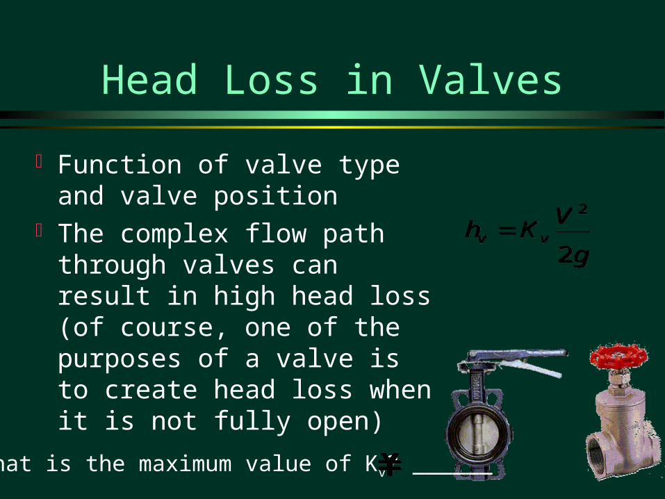
Head Loss in Valves

Function of valve type and valve position

The complex flow path through valves can result in high head loss (of course, one of the purposes of a valve is to create head loss when it is not fully open)

g

VKh vv

2

2

g

VKh vv

2

2

What is the maximum value of Kv? ______¥¥

Solution Technique: Head LossSolution Technique: Head Loss

Can be solved explicitly Can be solved explicitly

fl minorh h h= +å åfl minorh h h= +å å

2

2minor

Vh K

g=å

2

2minor

Vh K

g=å

2

f 2 5

8f

LQh

g Dp=

2

f 2 5

8f

LQh

g Dp=2

0.9

0.25f

5.74log

3.7 ReD

e=

é ùæ ö+ê úè øë û

2

0.9

0.25f

5.74log

3.7 ReD

e=

é ùæ ö+ê úè øë û

2

2 4

8minor

Q Kh

g Dp= å

2

2 4

8minor

Q Kh

g Dp= å

D

Q4Re

D

Q4Re

Solution Technique 1: Find D

Solution Technique 1: Find D

Assume all head loss is major head loss Calculate D using Swamee-Jain equation Calculate minor losses Find new major losses by subtracting minor

losses from total head loss

Assume all head loss is major head loss Calculate D using Swamee-Jain equation Calculate minor losses Find new major losses by subtracting minor

losses from total head loss

0.044.75 5.221.25 9.4

f f

0.66LQ L

D Qgh gh

e né ùæ ö æ ö

= +ê úç ÷ ç ÷è ø è øê úë û

42

28

Dg

QKhminor

42

28

Dg

QKhminor

f l minorh h h= - åf l minorh h h= - å

Solution Technique 2:Find D using Solver

Solution Technique 2:Find D using Solver

Iterative technique Solve these equations

Iterative technique Solve these equations

fl minorh h h= +å åfl minorh h h= +å å

42

28

Dg

QKhminor

42

28

Dg

QKhminor

2

f 2 5

8f

LQh

g Dp=

2

f 2 5

8f

LQh

g Dp=2

0.9

0.25f

5.74log

3.7 ReDe

=é ùæ ö+ê úè øë û

2

0.9

0.25f

5.74log

3.7 ReDe

=é ùæ ö+ê úè øë ûD

Q4Re

D

Q4Re

Use goal seek or Solver to find diameter that makes the calculated head loss equal the given head loss.

Spreadsheet

Exponential Friction FormulasExponential Friction Formulas

f

n

m

RLQh

D=f

n

m

RLQh

D=

units SI

675.10

units USC727.4

n

n

C

CR

units SI

675.10

units USC727.4

n

n

C

CR

1.852

f 4.8704

10.675 SI units

L Qh

D Cæ ö=è ø

1.852

f 4.8704

10.675 SI units

L Qh

D Cæ ö=è ø

C = Hazen-Williams coefficientC = Hazen-Williams coefficient

range of datarange of data

Commonly used in commercial and industrial settings

Only applicable over _____ __ ____ collected

Hazen-Williams exponential friction formula

Commonly used in commercial and industrial settings

Only applicable over _____ __ ____ collected

Hazen-Williams exponential friction formula

Head loss:Hazen-Williams Coefficient

Head loss:Hazen-Williams Coefficient

C Condition

150 PVC

140 Extremely smooth, straight pipes; asbestos cement

130 Very smooth pipes; concrete; new cast iron

120 Wood stave; new welded steel

110 Vitrified clay; new riveted steel

100 Cast iron after years of use

95 Riveted steel after years of use

60-80 Old pipes in bad condition

C Condition

150 PVC

140 Extremely smooth, straight pipes; asbestos cement

130 Very smooth pipes; concrete; new cast iron

120 Wood stave; new welded steel

110 Vitrified clay; new riveted steel

100 Cast iron after years of use

95 Riveted steel after years of use

60-80 Old pipes in bad condition

Hazen-Williams vs

Darcy-Weisbach

Hazen-Williams vs

Darcy-Weisbach

1.852

f 4.8704

10.675 SI units

L Qh

D Cæ ö=è ø

1.852

f 4.8704

10.675 SI units

L Qh

D Cæ ö=è ø

2

f 2 5

8f

LQh

g Dp=

2

f 2 5

8f

LQh

g Dp=

preferredpreferred

Both equations are empirical Darcy-Weisbach is dimensionally correct,

and ________. Hazen-Williams can be considered valid

only over the range of gathered data. Hazen-Williams can’t be extended to other

fluids without further experimentation.

Both equations are empirical Darcy-Weisbach is dimensionally correct,

and ________. Hazen-Williams can be considered valid

only over the range of gathered data. Hazen-Williams can’t be extended to other

fluids without further experimentation.

Air Release ValveAir Release Valve

http://www.ipexinc.com/industrial/airreleasevalves.html

http://www.apcovalves.com/airvalve.htm

PipesPipes

http://www.ipexinc.com/industrial/4080_pipe.html

Diameter O.D. Wall Thickness

I.D. Pressure 73°F

Wall Thickness

I.D. Pressure 73°F

(inches) (inches) (inches) (inches) (psi) (inches) (inches) (psi)

1/2 0.84 0.109 0.602 600 0.147 0.526 850

3/4 1.05 0.113 0.804 480 0.154 0.722 690

1 1.315 0.133 1.029 450 0.179 0.936 630

1 1/4 1.66 0.141 1.36 370 0.191 1.255 520

1 1/2 1.9 0.145 1.59 330 0.2 1.476 470

2 2.375 0.154 2.047 280 0.218 1.913 400

2 1/2 2.875 0.203 2.445 300 0.276 2.29 420

3 3.5 0.216 3.042 260 0.3 2.864 370

Schedule 40

PVC

Schedule 80

PVC

Additional PVC Pipe SchedulesAdditional PVC Pipe Schedules

http://www.prodigyweb.net.mx/pofluisa/pvc.htm#tubocementar

Presión de Trabajo

RD-13.5 22.4 kg/cm2 315 psi

RD-21 14.0 kg/cm2 200 psi

RD-26 11.1 kg/cm2 160 psi

RD-32.5 8.6 kg/cm2 125 psi

SurveyingSurveying

Vertical angle

r

x

z

cos2

x rp

qæ öD = -è ø

cos2

x rp

qæ öD = -è ø

sin2

z rp

qæ öD = -è ø

sin2

z rp

qæ öD = -è ø

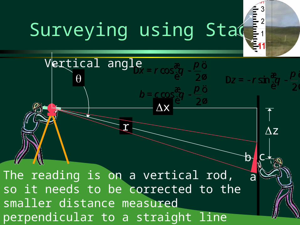
Surveying using StadiaSurveying using Stadia

Vertical angle

r

x

cos2

x rp

qæ öD = -è ø

cos2

x rp

qæ öD = -è ø sin

2z r

pqæ öD =- -

è øsin

2z r

pqæ öD =- -

è ø

The reading is on a vertical rod, so it needs to be corrected to the smaller distance measured perpendicular to a straight line connecting the theodolite to the rod.

a

z

b c

cos2

b cp

qæ ö= -è ø

cos2

b cp

qæ ö= -è ø

Horizontal DistanceHorizontal Distance

cos2

x rp

qæ öD = -è ø

cos2

x rp

qæ öD = -è ø

cos2

b cp

qæ ö= -è ø

cos2

b cp

qæ ö= -è ø

sin cos2p

q qæ ö= -è ø

sin cos2p

q qæ ö= -è ø

Trig identity

sinx r qD = sinx r qD =

sinb c q= sinb c q=

r Mb=r Mb= M is the Stadia multiplier (often 100)

( )2sinx Mc qD = ( )2sinx Mc qD = c is the Stadia reading

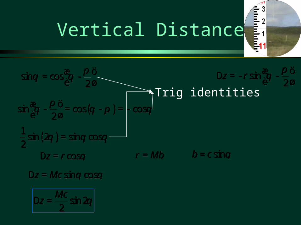
Vertical DistanceVertical Distance

sin2

z rp

qæ öD =- -è ø

sin2

z rp

qæ öD =- -è ø

( )sin cos cos2p

q q p qæ ö- = - =-è ø

( )sin cos cos2p

q q p qæ ö- = - =-è ø

sin cos2p

q qæ ö= -è ø

sin cos2p

q qæ ö= -è ø

sinb c q= sinb c q=r Mb=r Mb=

sin cosz Mc q qD = sin cosz Mc q qD =

( )1sin 2 sin cos

2q q q=( )1

sin 2 sin cos2

q q q=

cosz r qD = cosz r qD =

sin 22

Mcz qD = sin 2

2Mc

z qD =

Trig identities

Pipe Length (along the slope)Pipe Length (along the slope)

r Mb=r Mb= sinb c q= sinb c q=

sinr Mc q= sinr Mc q=