Monopolistic Competition in Trade II: 2-by-2 Model …users.ox.ac.uk/.../lecture_notes/09_Monopolistic_Competition_II.pdf · Monopolistic Competition in Trade II: 2-by-2 Model and

Monopolistic Competition in Trade II:2-by-2 Model and Transport CostsNotes for Oxford M.Phil. International Trade

J. Peter Neary

University of Oxford

November 24, 2011

J.P. Neary (University of Oxford) Monopolistic Competition II November 24, 2011 1 / 22

Plan of Lectures

1 Two-by-Two Model with Monopolistic Competition

2 Transport Costs


Two-by-Two Model with Monopolistic Competition

Plan of Lectures

1 Two-by-Two Model with Monopolistic CompetitionDixit-Stiglitz “Lite” PreferencesFactor-Price EqualisationThe FPE SetThe FPE Set and Inter-Industry TradeIntra-Industry TradeIIT without Inter-Industry TradeIntra-Industry Trade off the DiagonalLoci of Constant Intra-Industry TradeEmpirical Work on Monopolistic Competition and TradeTrade and Income Distribution

2 Transport Costs


Two-by-Two Model with Monopolistic Competition Dixit-Stiglitz “Lite” Preferences

Dixit-Stiglitz “Lite” Preferences

Extend 2-by-2 HO Model by assuming that one sector has aDixit-Stiglitz monopolistically competitive structure

2 sectors:

XF : ”Food”: homogeneous good, perfect competition, pF = 1XM : ”Manufactures”: differentiated goods, monopolistic competition

Preferences: [“Dixit-Stiglitz Lite”]

U = X1−µF X

µM , XM =

(Σix

σ−1σ

i

) σσ−1

U is “homothetically separable”, so “two-stage budgeting” is justified:Stage 1: Max U subject to: XF + PXM = I

(pF = 1; P is the price index dual to the sub-utility function XM)⇒ XF = (1− µ)I , XM = µ I

PStage 2: Max XM subject to: Σipixi = µI

⇒ xi = x = ( pP )−σ µI

P , as in earlier one-sector application.

Hence, y and p fixed by σ and costs as in one-sector case.


Two-by-Two Model with Monopolistic Competition Factor-Price Equalisation

Factor-Price Equalisation

FPE holds just as in perfectly competitive model:Food: Free entry and exit equalises output price and AC, andprofit-maximizing minimizes average cost:

1 = cF (w , r) = aLFw + aKF r (1)

Manufacturing: With homotheticity (fixed and variable costs use thesame factor proportions), total costs for firm i are:

Ci = (f + ayi ) cM (w , r) cM (w , r) = aLMw + aKM r (2)

Pricing condition for each monopolistically competitive firm is asbefore, except that MC depends on the costs of both factors ofproduction:

p =σ

σ− 1(aLMw + aKM r) (3)

Apart from σ, equations (1) and (3) are identical to the correspondingequations in the perfectly competitive Heckscher-Ohlin model.So, as there, they form a sub-system which determines factor pricesgiven the relative price of manufactures p.


Two-by-Two Model with Monopolistic Competition The FPE Set

The FPE Set

As in competitive case, all allocations in the FPE set replicate theintegrated equilibrium:

How come, with increasing returns in one sector?Because of CES preferences: y fixed, only n to be determined

Full employment conditions:

L = aLFYF + aLM (f + ay) n, K = aKFYF + aKM (f + ay) n (4)

aij fixed by FPE; a and f by assumption; y by free entry and CES.So: two linear equations in two unknowns YF and n.

Hence, just as in perfectly competitive Heckscher-Ohlin model:All factor allocations in FPE set generate the same world outputs:

(4) with L = LW and K = KW determine YWF and N = n+ n∗

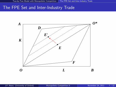
Rybczynski Theorem holds, determining outputs YF and YM = ny asfunctions of factor endowments from (4).Heckscher-Ohlin Theorem also holds: Consumption always alongdiagonal, so volume of inter-industry trade depends on differences infactor endowments only.


Two-by-Two Model with Monopolistic Competition The FPE Set and Inter-Industry Trade

The FPE Set and Inter-Industry Trade

O*A OD

E'

A

KE'

E

F

LO B


Two-by-Two Model with Monopolistic Competition Intra-Industry Trade

Intra-Industry Trade (IIT)

In addition, consumers’ taste for diversity drives IIT in manufactures.Special case: points along the diagonal OO∗:

No inter-industry trade, and so no net trade in manufacturesNevertheless, there is IIT, as consumers at all locations demand bothhome and foreign varieties of manufactures.HO model reduces to a one-factor model with n

N = LL+L∗ =

KK+K ∗ .

Total value of IIT: VIIT = 2M [M: value of home’s imports].M = θIIT I [θIIT : share of home spending I on imported manufactures].θIIT = µ n∗

N in general; = L∗

L+L∗ along OO∗.I = wL+ rK = (w + rk) L.

So: VIIT = 2M = 2µ

L+L∗ (w + rk) LL∗ = 2µ

LW(w + rk) L(LW − L).

w and r fixed by FPE, k fixed by slope of OO∗, LW assumed fixed

So VIIT is proportional to L(LW − L); this is maximized at L = LW

2 .When the countries are of equal size, each exports exactly half theoutput of its manufacturing sector.At a point on OO∗ closer to O∗, say E ′′, home produces more varietiesand so imports fewer. Hence VIIT is lower.


Two-by-Two Model with Monopolistic Competition IIT without Inter-Industry Trade

IIT without Inter-Industry Trade

O*OD

K E"

E

F

LO


Two-by-Two Model with Monopolistic Competition Intra-Industry Trade off the Diagonal

Intra-Industry Trade off the Diagonal

Next: points off the diagonal OO∗:VIIT = 2M = 2µ n∗

N I = 2µ n∗N (wL+ rK ); µ, N, w , r fixed in FPE set;

n∗ is linear in L and K ;hence iso-VIIT loci define K as a quadratic function of L.e.g.: move away from E along a line with slope −w/r so I constant

dI = wdL+ rdK = 0 if dK = −wr dL

At E ′, n∗ is lower by the Rybczynski effect.Hence home imports fewer varieties, so IIT is lower.

Bottom-line conclusions: Two types of trade coexist:

Inter-industry: driven by differences in comparative advantage.Intra-industry: encouraged by similarities in country size.


Two-by-Two Model with Monopolistic Competition Loci of Constant Intra-Industry Trade

Loci of Constant Intra-Industry Trade

O*OD

E'K

E'E"

E

F

LO


Two-by-Two Model with Monopolistic Competition Empirical Work on Monopolistic Competition and Trade

Empirical Work on Monopolistic Competition and Trade

Grubel-Lloyd (1975): Finding of pervasive IIT inspired theory.

Helpman (JJIE 1987):

Empirical implications of monopolistically competitive model: a gravityequation very similar to the Anderson one.Consistent with manufacturing trade between advanced economies.

Hummels-Levinsohn (QJE 1995):

Gravity works equally well for trade flows between non-OECD countries.

Evenett-Keller (JPE 2002):

Gravity equation works better for countries with a higher share of IIT.

Rauch (JIE 1999): Classification of traded goods:

Gravity model works better for differentiated goods.


Two-by-Two Model with Monopolistic Competition Trade and Income Distribution

Trade and Income Distribution

Finally: Stolper-Samuelson still holds in a sense.

Difference: real factor rewards depend on true price index.

This is overestimated by the common price of manufactures.

In particular: Gains from greater diversity accrue to all.

This may offset magnification effect of S-S.

This may explain findings of Balassa (1967) that adjustment togrowing trade in postwar Western Europe led to little distributionalconflict.


Transport Costs

Plan of Lectures

1 Two-by-Two Model with Monopolistic Competition

2 Transport CostsPricingPrice Index EffectPrice Index Effect: FigureGoods-Market EquilibriumPrice Indexes and Relative IncomesPrice Indexes and Relative Incomes: FigureThe Price-Index and Home-Market Effects: FigureThe Home-Market Effect


Transport Costs Pricing

Pricing

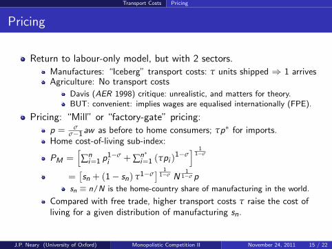
Return to labour-only model, but with 2 sectors.

Manufactures: “Iceberg” transport costs: τ units shipped ⇒ 1 arrivesAgriculture: No transport costs

Davis (AER 1998) critique: unrealistic, and matters for theory.BUT: convenient: implies wages are equalised internationally (FPE).

Pricing: “Mill” or “factory-gate” pricing:

p = σσ−1aw as before to home consumers; τp∗ for imports.

Home cost-of-living sub-index:

PM =[∑ni=1 p

1−σi + ∑n∗

i=1 (τpi )1−σ] 1

1−σ

=[sn + (1− sn) τ1−σ

] 11−σ N

11−σ p

sn ≡ n/N is the home-country share of manufacturing in the world.

Compared with free trade, higher transport costs τ raise the cost ofliving for a given distribution of manufacturing sn.


Transport Costs Price Index Effect

Price Index Effect

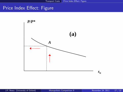
Next: More important is the effect of changes in sn itself:

A rise in sn means that home consumers save on transport costs.(They purchase more domestic varieties and fewer imported ones)Hence the true cost of living falls.Opposite is true in the foreign country.

P = P1−µF P

µM , PF common; so: P

P∗ =(PMP∗M

)µ.

Hence there is a negative relationship between the relative cost ofliving at home and abroad, P/P∗, and the home-country share ofmanufacturing sn:

P

P∗=

[sn + (1− sn) τ1−σ

(1− sn) + snτ1−σ

] µ1−σ

(5)

This is illustrated by the downward-sloping locus in Figure.


Transport Costs Price Index Effect: Figure

Price Index Effect: Figure

(a)

P/P*

A

sn


Transport Costs Goods-Market Equilibrium

Goods-Market Equilibrium

Implications of goods-market equil. with fixed factory-gate prices:

Demand facing a typical domestic firm:

x =

(p

PM

)−σ µI

PMx∗ =

(τp

P∗M

)−σ µI ∗

P∗M(6)

N.B. Price paid by foreign consumers is grossed up by transport costs.So: Total sales equal x + x∗?NO: Shipments to the foreign market exceed foreign demand forimports x∗ because of the wastage incurred in transit.Hence market-clearing condition for a typical home-produced variety:

y = X = x + τx∗ = µp−σ[IPσ−1

M + τ1−σI ∗ (P∗M )σ−1]

(7)

From the firm’s partial-equilibrium perspective, [.] is exogenous, so thedemand it faces is a simple iso-elastic function of the price it charges,with incomes, price indices, and transport costs given.However, in GE, y and p are fixed and the same in each country as wehave seen, so incomes and price indices must adjust to ensure thatgoods markets clear.


Transport Costs Price Indexes and Relative Incomes

Price Indexes and Relative Incomes

Home: y = X = x + τx∗ = µp−σ[IPσ−1

M + τ1−σI ∗ (P∗M)σ−1]

Corresponding equation for foreign firms:

y∗ = X ∗ = x∗ + τx = µp−σ[I ∗(P∗M)σ−1

+ τ1−σIPσ−1M

]Combining, with y = y∗:

IPσ−1M + τ1−σI ∗

(P∗M)σ−1

= I ∗(P∗M)σ−1

+ τ1−σIPσ−1M

⇒(1− τ1−σ

)IPσ−1

M =(1− τ1−σ

)I ∗(P∗M)σ−1

⇒ sI = (1− sI )(PMP∗M

)1−σ

where sI ≡ I/ (I + I ∗) is the home-country share of world income.⇒ required negative relationship between relative price indexes andrelative incomes:

P

P∗=

(sI

1− sI

) µ1−σ

(8)

This is illustrated by the downward-sloping locus in figure.


Transport Costs Price Indexes and Relative Incomes: Figure

Price Indexes and Relative Incomes: Figure

P/P*

B

(b)

sI


Transport Costs The Price-Index and Home-Market Effects: Figure

The Price-Index and Home-Market Effects: Figure

P/P*

AB

(a)(b)

A'B'

snsI


Transport Costs The Home-Market Effect

The Home-Market Effect

Combining the two panels, initial equilibrium at A and B:Exogenous shock raises home relative income: left arrow in panel (b).From panel (b), for goods markets to return to equilibrium, homecountry must experience a fall in its relative price level.But then, from (a), it must also acquire a larger share of worldmanufacturing.

N.B. Curve in (a) less elastic than that in (b): relative price indices aremore responsive to home’s share of income than of manufacturing.(5) and (8) only coincide with infinite transport costs (τ1−σ = 0) : inautarky, home shares of world manufacturing and income must beequal.

Formally, as in HK (1985), equations (5) and (8) can be solved:

P

P∗=

[sn + (1− sn) τ1−σ

(1− sn) + snτ1−σ

] µ1−σ

=

(sI

1− sI

) µ1−σ

(9)

to give a linear relationship between manufacturing and income shares:

sn =(1 + φ) sI − φ

1− φ, where: φ ≡ τ1−σ (10)


Monopolistic Competition in Trade II: 2-by-2 Model …users.ox.ac.uk/.../lecture_notes/09_Monopolistic_Competition_II.pdf · Monopolistic Competition in Trade II: 2-by-2 Model and

Documents