Monocular Depth Ordering Using T-Junctions and Convexity Occlusion Cues

1926 IEEE TRANSACTIONS ON IMAGE PROCESSING, VOL. 22, NO. 5, MAY 2013

Monocular Depth Ordering Using T-Junctions andConvexity Occlusion Cues

Guillem Palou, Student Member, IEEE, and Philippe Salembier, Fellow, IEEE

Abstract— This paper proposes a system that relates objectsin an image using occlusion cues and arranges them accordingto depth. The system does not rely on a priori knowledge ofthe scene structure and focuses on detecting special points,such as T-junctions and highly convex contours, to infer thedepth relationships between objects in the scene. The systemmakes extensive use of the binary partition tree as hierarchicalregion-based image representation jointly with a new approachfor candidate T-junction estimation. Since some regions maynot involve T-junctions, occlusion is also detected by examiningconvex shapes on region boundaries. Combining T-junctions andconvexity leads to a system which only relies on low level depthcues and does not rely on semantic information. However, itshows a similar or better performance with the state-of-the-artwhile not assuming any type of scene.

As an extension of the automatic depth ordering system, asemi-automatic approach is also proposed. If the user providesthe depth order for a subset of regions in the image, the systemis able to easily integrate this user information to the finaldepth order for the complete image. For some applications, userinteraction can naturally be integrated, improving the quality ofthe automatically generated depth map.

Index Terms— Binary partition tree (BPT), convexity, monoc-ular depth, occlusion cues, T-junction estimation.

I. INTRODUCTION

HUMANS are known for their ability to recognize objectsand determine the scene structure in many distinct situ-

ations. Our capacity to retrieve a coherent depth interpretationof the environment seems to be robust and reliable in themajority of cases, with the exception of some optical illusions.The ability to perceive a 3-D world in humans is mainly due tobinocular vision, where each eye provides a different image ofthe scene and disparity is subconsciously inferred. However,in monocular situations, perception is affected but still, depthinformation can be perceived. The scientific community hastried to mimic the human behavior to determine the depthstructure of scenes. To this day, human performance is stillmuch better than computer based approaches in both timeand accuracy, but the evolution of 3-D visualization hardwareencourages researchers devote efforts to estimate depth fromvisual content.

Manuscript received January 2, 2012; revised December 17, 2012; acceptedJanuary 5, 2013. Date of publication January 14, 2013; date of currentversion March 14, 2013. The associate editor coordinating the review of thismanuscript and approving it for publication was Prof. Kenneth Lam.

G. Palou and P. Salembier are with the Signal Theory and CommunicationsDepartment at the Technical University of Catalunya, Barcelona 08034, Spain(e-mail: [email protected]; [email protected]).

Color versions of one or more of the figures in this paper are availableonline at http://ieeexplore.ieee.org.

Digital Object Identifier 10.1109/TIP.2013.2240002

With the decrease of stereo camera costs, depth estimationin stereo/multiview systems is gaining more importance. Mostof the state of the art systems on depth estimation take profitof multiple points of view to infer disparity. However, mostof the acquired content has only one point of view. The hugeamount of photos or movies obtained with conventional cam-eras makes monocular depth estimation an attractive researcharea and an rather pressing need for the 3-D media industry.As 2-D to 3-D conversion is a relatively new field, manysystems still rely on semi-supervised approaches to correctestimation errors. For example, converting monocular contentto 3-D to some extend has been an objective for manyindustrial actors such as Microsoft [1], Disney [2] or PrimeFocus (a post-production company for Hollywood Studios)with View-D software [3]. Monocular depth systems are notable to estimate a perfect depth map, but, in practice, arough representation may suffice for humans to perceive a3-D effect [4]. Additionally, monocular depth estimation canbe used as an input to other systems such as object editing bydepth (foreground/background removal, or example) or as a arough depth estimation for a full 3-D system.

Although current commercial products (such as the onespreviously mentioned) heavily rely on human interaction toderive a correct depth interpretation, there is a need for anautomated system to reduce both time and costs. To thisend, many research institutions [5], [6] have proposed severalmonocular depth estimation systems. These systems basetheir reasoning on finding monocular depth cues in images.Although these cues are easily identified by humans, they area detection challenge for state of the art computer algorithms.Since they are an important part of the proposed algorithm,Section I-A is devoted to describe their role on human depthperception. Section I-B discusses the current literature onmonocular depth estimation, followed by a brief descriptionof the structure and innovations of our system.

A. Monocular Low Level Depth Cues

Perceptual organization is a widely known area of studyin the Gestalt Psychology with its Laws of Organization.According to this field, the set of cues that humans use toinfer depth in a single image [7], are, among others: bright-ness, shading, blurring, occlusion, convexity, vanishing points,texture gradient and familiar size. Even though humans makeextensive use of stereo vision to perceive absolute depth, whenonly one point of view is available, we are also capable to infercertain depth relationships. Many monocular cues also rely on

1057-7149/$31.00 © 2013 IEEE

PALOU AND SALEMBIER: MONOCULAR DEPTH ORDERING USING T-JUNCTIONS AND CONVEXITY OCCLUSION CUES 1927

(a) (b) (c) (d)

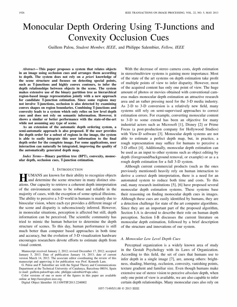
Fig. 1. (a) T-junction example. Locally, region R2 is the one forming the largest angle, appearing to be over R1 and R3. (b) Inverted T-junction example.Locally, region R1 is the one forming the largest angle, but corresponds to the sky region, which is behind the dog. (c) and (d) Points of high convexity arecues to determine the relative depth. Local cues at each boundary point should be averaged to decide the correct sign of convexity.

the overall scene knowledge and previously known situationssuch as the sun being on top or people standing upright onthe ground. A priori knowledge of the scene structure, likethe approximate size of a person or the shape of a tree mayalso help to infer depth in natural scenes. Other cues, such asocclusion, are local and related to specific image points. Atthese points, the image structure may offer good signs of depthdiscontinuity. Produced by the projection of the 3-D scene intothe image plane, occlusion is specially observed in two cases:T-junctions and convexity.

T-junction points appear when an object is in front ofother two objects, see Fig. 1. T-junctions are formed bythree regions and, locally, one of them is forming an almostflat angle (i.e. 180 degrees). The other two regions mayform two arbitrary angles, but if any falls below 30-40degrees, the perception of occlusion falls rapidly [8]. AlthoughT-junctions are clear signs of occlusion, the relative depthorder of the intervening regions cannot be determined exclu-sively by examining the local angle configuration. In normalT-junctions, the region forming the largest angle is likely to bethe occluding region (and thus closer to the viewer). However,in the case of inverted T-junctions, the same region cancorrespond to the background (and thus occluded and furtheraway to the viewer). According to [8], junction detection isdifficult even for humans but, once detected, the occludingside is easily identified, see Fig. 1(b). Computers, howeverhave much more difficulties in determining the depth orderand a global reasoning on other T-junctions is needed.

The second case of occlusion is produced when a singleobject is lying in front of other regions. In small neigh-borhoods of the object boundaries, convex shapes appear tobe in front of their background, whether or not other cuesare present. When humans deal with natural shapes, localdecisions at points of object boundaries are averaged alongthe entire object contour to arrive at a global interpretation.For example, in Fig. 1(c), a feline standing in front of a wallis shown. If convexity is interpreted along the boundariesas shown in Fig. 1(d), there may be parts of the contourindicating one depth order (green arrows) and other parts withopposite sign (red arrows). In such cases, humans partially useconvexity cues to decide that the feline is in front of the wall.As a priori information, recognizing the different parts of theimage (the feline and the wall) immediately restricts the scenestructure. Humans know that a feline cannot be visible andbehind a wall at the same time. Nevertheless, occlusion cueshelp to enforce depth relationships even in known situations.

Humans not only make use of local cues to derive thedepth structure of an image, but other global reasoningstake place. Therefore, it is unlikely that a system for depthperception defined only on T-junction and convexity detectioncan compete with human vision. However, in this paper, weare interested in studying the performances and limitationsof such a system. In cases where the system cannot achievethe correct depth interpretation, user interaction can be used.Since humans can easily identify depth planes in an image,the proposed system incorporates the possibility to acceptdepth information on a limited set of regions provided withmarkers defined by the user. Markers are widely used in imageprocessing: image segmentation [9], reconstruction [10] or 2-Dto 3-D reconstruction [4]. In this work, markers set the depthrelations on image regions.

B. Related Work

Monocular depth perception is a fairly new field of studyin computer vision. One of the first works trying to recoverthe image structure was presented in [11], but reference pointswere needed to reconstruct lines and planes. In [12], insteadof the overall depth organization, a computation of the scaleof the image (i.e. mean depth) was proposed. Focusing onalgorithms that recover absolute/relative depth of regions inthe image, two main approaches are found. The ones that usehigh level information and the ones that operate over the imagestructure finding special points indicating some depth cues. Inthe former class, [5] and [6] oversegment the image and gatherfor each region color, texture, vertical and horizontal featuresto use them in a conditional random field, trained a priori witha ground truth data set, for absolute depth estimation. The maindrawback of high-level information approaches is that they arelimited to the kind of images they have been trained for. Thelatter type of systems, where [13] can be included, use focuson the detection of relative depth cues such as occlusion toorder the objects in the scene. Occlusion does not permit toinfer absolute depth as high-level information may offer, butis more generic as it does not assume anything about the typeof scene.

Depth ordering the regions of an image permits to determineimmediately the occlusion boundaries. An occlusion boundaryis defined as the border between two different depth planes.Moreover, the nearest side of the boundary is defined as theowner (or figure, foreground) of the boundary. Similarly, itsfurther side is called the background or simply, ground, of


the boundary. The problem to detect on occlusion boundarieswhich side is figure and which side is ground has beenaddressed by works in [14]– [16]. Similar to depth estimationsystems, some of these approaches rely also on low level cuessuch as shapemes [14], convexity or parallelism [15]. The maindrawback of these systems is that they do not provide closedpartitions and only single contours are labeled.

Following the computational vision model of [17], [18],our system tries to integrate the estimation of depth cuesand the segmentation process. In this work, the segmentationis understood as a two step process: A construction of aregion-based, hierarchical representation of the image, and aselection of the regions in this hierarchy to compose the finaldepth ordered partition. Inside this framework, T-junction andconvexity cues are estimated iteratively during the first step ofthe system. The second stage proposes an optimization schemeto produce a depth ordered partition from the depth relationsdetermined by the previously mentioned cues.

This architecture differs from the one of [13], which consistsof an estimation of T-junction points, followed by imagesegmentation, convexity detection and a final depth orderingstage. Here we integrate the estimation of low level depth cuesinto the construction of the BPT. As the framework is region-based, our aim is to increase the performance and robustnessof the cue detection compared to [13] where the T-junctiondetection is performed using a modification of the [19] pixel-based detector. A part from the architecture, another funda-mental difference with [13] is that the T-junction model isextended to include both normal and inverted depth orders.Finally, the last major difference deals with the pruning of theBPT, formulated here as an optimization problem on the tree.

Although the system can provide an automatic depthordered segmentation of the image, an optional strategyinvolving user interaction is also discussed. The purpose ofincorporating human interaction is to help the system to decidein challenging situations, where the assumptions related to lowlevel depth cues are not fulfilled. To interact with the system,a few depth markers can be provided as an additional input. Ifthat is the case, the depth relations introduced by the user arenaturally combined with the detected depth cues in the secondstage of the system. This form of interaction is suitable owingto the fact that the first step of the system is computationallymore costly. As a result, with little computation overload, theuser is able to easily refine the markings in case the algorithmdoes not provide a sufficiently accurate solution. The workin [4] also proposes algorithms for semi-automatic 2-D to3-D reconstruction, for videos and single images. These sys-tems offer absolute depth maps (up to a scale), while oursystem outputs relative depth orders.

Two major conclusions can be drawn from this work: First,it is shown that using only low-level (and very local) cues aglobal depth ordering of the image can be obtained. Second, itis shown that even if the algorithm does not rely on a trainingphase, results are of similar or better quality than approachesof the state of the art [5], [6] that rely on high level specific(even semantic) cues.

The following sections describe the system architecture.First, the system models are exposed in Section II, as well as

how the hierarchical image representation is built. Section IIIis devoted to the estimation of occlusion cues. Section IVdescribes the process of finding a suitable depth orderedpartition from the set of estimated cues. Finally, experimentalresults are presented in Section V for both the automaticand the semi-automatic proposed systems. Comparison withother systems is also performed qualitatively against [5], [6],and [13] and quantitatively with [14], [15] by evaluating theperformance on occlusion boundaries.

II. SYSTEM MODELS

An important part of the system relies on the BinaryPartition Tree (BPT). The BPT is a structured hierarchicalrepresentation of the image regions that can be obtainediteratively from an initial partition [20], [21]. At each iteration,pairs of adjacent regions are iteratively merged to form aparent region containing the two merged ones [20]. The pairof regions to be merged are the two most similar accordingto a similarity measure. In this project, the BPT is used withtwo objectives:

1) Region-based representation of the image: Pixels can bethought as the basic unit of image information. Manytimes working with pixels is limiting and another imagerepresentation is needed. In our case the final objective isto have a depth ordering of objects/regions in the imageso, a region representation is needed. Going from pixelsto regions is carried out using the BPT algorithm

2) Solution space: When the BPT is constructed, the leavesof the tree represent the regions belonging to the initialpartition and the root node refers to the entire imagesupport. The remaining tree nodes represent the inter-mediate regions formed during the merging process.Many partitions can be formed by combining regionsrepresented in this hierarchical structure. This processcan be seen as a tree pruning. In summary, the BPTdefines a partition solution space.

A. Region Model

To define similarity, region models are needed, along witha distance measure between them. The chosen color spaceto represent the image is the C I E Lab because of theperceptual nature of color difference metrics in this space.Region color distribution is modeled using adaptive three-dimensional histograms (signatures), [22]. Previous regionmerging algorithms use a simpler region model, consideringonly the mean color [21] or monodimensional histograms [23].3-D-histograms do not loose correlation information betweenchannels. Unfortunately, their representation is very costly inmemory usage. To overcome this drawback, adaptive signa-tures as in [22] are chosen. In practice, 8 dominant colors area good choice to represent the whole image [24], so the samenumber is chosen to describe each region, but depending onthe region color homogeneity, a lower number may suffice.Each signature si is characterized by a set of ordered pairs{(p1, c1), (p2, c2) . . . (pn, cn)} with n ≤ 8. Each pair i iscomposed of a representative color vector ci and its probabilityof appearance pi . Since in a BPT construction, some regions


belong to the initial partition and some others are created bymerging, the estimation of these dominant colors is dependingon the nature of the region. If the initial partition is formedby individual pixels, the dominant color for each region issimply the pixel color. If a segmentation is available as input,the dominant colors of the regions containing many pixelsare estimated using a quantization algorithm as in [25]. In ourcase, the proposed system has no segmentation input, thereforethe initial partition is formed by the pixels. On the other hand,when a region is the result of a merging process, anotherapproach can be followed to reduce the computational burden.

Hierarchical Signature Estimation: To approximate a jointsignature s from two signatures si and s j , the followingalgorithm is proposed: When two regions are merged, a newsignature s is created for the parent region by joining thetwo underlying signatures, si and s j . While the number ofrepresentative colors exceeds the maximum (that is 8, here),the two most similar colors are merged and replaced by theiraverage color, until s contains at most 8 colors.

The distance di j chosen to measure the difference betweentwo colors i and j of signature s is di j = (pi + p j )ci j . Wherethe ci j term is perceptually defined as in [22] which is basedin [26]:

ci j =(

1 − e− �i jγ

)(1)

with �i j being the euclidean distance between Lab-colors ci

and c j . The decay parameter γ indicates a soft threshold ofdistinguishable colors and is set to 14.0 as in [22].

B. Region Similarity Measure

The construction of the BPT is done by merging neighbor-ing regions iteratively. The order in which these regions aremerged is defined by a similarity measure. Usually, this mea-sure is based on low-level features of the regions such as color,area, or shape [21]. In this work, however, depth informationbased on T-junctions is also introduced to contribute to thismeasure. The formal expression used to measure the similaritybetween two adjacent regions R1 and R2 is:

d(R1, R2) = da (αdc + (1 − α)ds) dd (2)

da stands for the area distance. dc and ds are the colorand shape measures respectively. α is the weighting factorbetween shape and color and its value was experimentallyset to α = 0.7, giving color much more importance thanshape. dd is the newly introduced depth measure. These fourcontributions (area,color,shape and depth) are considered to bekey characteristics to define regions.

Color has been proven to be the most important feature. Inpractice, however, objects in the real world have more or lesscompact and round shapes. The exclusive use of color distancedc lead to regions with unnatural shapes so a measure eval-uating the region shape ds is introduced. Moreover, relevantobjects in a scene present similar areas so a term addressingregion size da is also included. Since the goal of this workis to estimate depth planes, the inclusion of a depth measuredd attempts to differentiate different levels of depth alreadyduring the BPT construction.

To measure color similarity dc(R1, R2) between signatures,the earth mover’s distance (EMD) [27] is chosen:

dc(R1, R2) = E M D(s1, s2). (3)

Although in [22] this distance is used locally to detect cornersand junctions, there is no knowledge that it has been used for acomplete segmentation process. The EMD distance is definedto be the minimum cost to transport a certain probabilitymasses fi j to transform one signature s1 to another s2,according to some costs between signature colors. Formally,the EMD is defined as:

E M D(s1, s2) = min∑

i

∑j

fi j ci j (4)

subject to: fi j ≥ 0,∑

i

fi j = p2 j ,∑

j

fi j = p1i . (5)

The costs ci j are defined as the distance (1) betweensignature colors. The constraints (5) impose that the probabil-ity masses fi j should be non-negative and should transformthe probabilities of occurrence in s1 (p11, p12, . . . , p1n) tothe ones in s2, (p21, p22, . . . , p2n). The minimization of (4)subject to (5) is performed using linear programming [28].The shape distance is the relative increase of perimeter of thenew region with respect to the biggest one [21]:

ds(R1, R2) = max

(0,

min(P1, P2) − 2P1,2

max(P1, P2)

)(6)

where P1, P2 and P1,2 are the two region perimeters and thecommon perimeter respectively. ds is only applied when bothregion shapes are meaningful (i.e. at least 50 pixels in area).

The area distance is defined as:da(R1, R2) = log (1 + min(A1, A2)) (7)

with A1, A2 the respective region areas in pixels. There isno general consensus about which area weighting distanceshould be used during BPT construction. In [21], [23], eitherno weighting and linear weighting are performed. Generally,area weighting is used to encourage the merging of smalland semantically unimportant regions before the large regionsmerge. In this work, a logarithmic weighting is chosen.

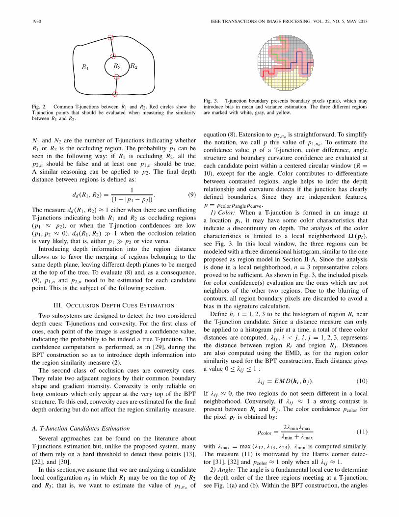
As a final similarity measure, depth information dd isintroduced using T-junction candidate points. The idea isto increase the region distance if two adjacent regions donot belong to the same depth plane, according to a set ofT-junctions. To determine the probability that a region R1occludes R2, common T-junction candidate points are exam-ined. Candidates arise where three regions meet, see Fig. 2.

If R1 and R2 share a common neighbor R3, at least aT-junction candidate n is present at the contact point(s) of thethree regions. For each candidate n a probability pi,n , i = 1, 2,of the occluding region to be Ri is computed as described inSection III. Common candidates between R1 and R2 determinethe probability of occlusion:

px =(

1 −Nx∏n

(1 − px,n

)) Ny∏n

(1 − py,n

)(8)

where (x, y) = (1, 2) or vice versa. Therefore, p1, p2 is theprobability of R1, R2 being the occluding region respectively.


R1 R2R3

Fig. 2. Common T-junctions between R1 and R2. Red circles show theT-junction points that should be evaluated when measuring the similaritybetween R1 and R2.

N1 and N2 are the number of T-junctions indicating whetherR1 or R2 is the occluding region. The probability p1 can beseen in the following way: if R1 is occluding R2, all thep2,n should be false and at least one p1,n should be true.A similar reasoning can be applied to p2. The final depthdistance between regions is defined as:

dd(R1, R2) = 1

(1 − |p1 − p2|) . (9)

The measure dd(R1, R2) ≈ 1 either when there are conflictingT-junctions indicating both R1 and R2 as occluding regions(p1 ≈ p2), or when the T-junction confidences are low(p1, p2 ≈ 0). dd(R1, R2) � 1 when the occlusion relationis very likely, that is, either p1 � p2 or vice versa.

Introducing depth information into the region distanceallows us to favor the merging of regions belonging to thesame depth plane, leaving different depth planes to be mergedat the top of the tree. To evaluate (8) and, as a consequence,(9), p1,n and p2,n need to be estimated for each candidatepoint. This is the subject of the following section.

III. OCCLUSION DEPTH CUES ESTIMATION

Two subsystems are designed to detect the two considereddepth cues: T-junctions and convexity. For the first class ofcues, each point of the image is assigned a confidence value,indicating the probability to be indeed a true T-junction. Theconfidence computation is performed, as in [29], during theBPT construction so as to introduce depth information intothe region similarity measure (2).

The second class of occlusion cues are convexity cues.They relate two adjacent regions by their common boundaryshape and gradient intensity. Convexity is only reliable onlong contours which only appear at the very top of the BPTstructure. To this end, convexity cues are estimated for the finaldepth ordering but do not affect the region similarity measure.

A. T-Junction Candidates Estimation

Several approaches can be found on the literature aboutT-junctions estimation but, unlike the proposed system, manyof them rely on a hard threshold to detect these points [13],[22], and [30].

In this section,we assume that we are analyzing a candidatelocal configuration no in which R1 may be on the top of R2and R3; that is, we want to estimate the value of p1,no of

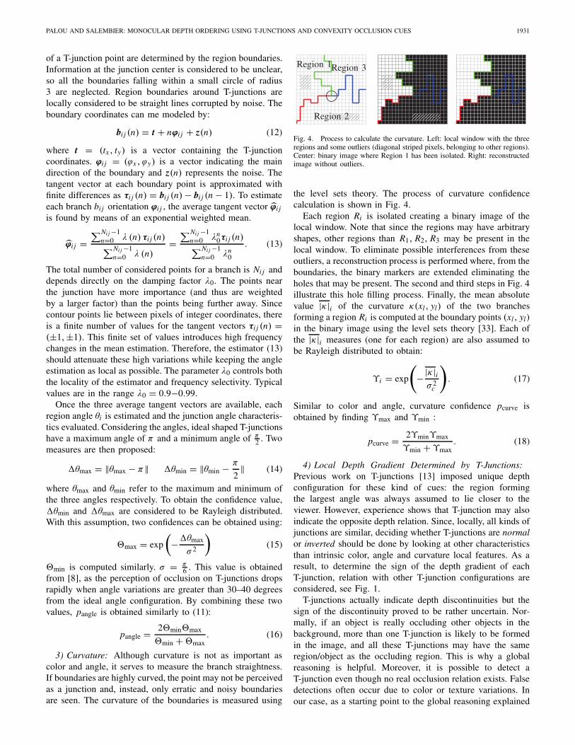
Fig. 3. T-junction boundary presents boundary pixels (pink), which mayintroduce bias in mean and variance estimation. The three different regionsare marked with white, gray, and yellow.

equation (8). Extension to p2,no is straightforward. To simplifythe notation, we call p this value of p1,no . To estimate theconfidence value p of a T-junction, color difference, anglestructure and boundary curvature confidence are evaluated ateach candidate point within a centered circular window (R =10), except for the angle. Color contributes to differentiatebetween contrasted regions, angle helps to infer the depthrelationship and curvature detects if the junction has clearlydefined boundaries. Since they are independent features,p = pcolor pangle pcurve.

1) Color: When a T-junction is formed in an image ata location pt , it may have some color characteristics thatindicate a discontinuity on depth. The analysis of the colorcharacteristics is limited to a local neighborhood � ( pt),see Fig. 3. In this local window, the three regions can bemodeled with a three dimensional histogram, similar to the oneproposed as region model in Section II-A. Since the analysisis done in a local neighborhood, n = 3 representative colorsproved to be sufficient. As shown in Fig. 3, the included pixelsfor color confidence(s) evaluation are the ones which are notneighbors of the other two regions. Due to the blurring ofcontours, all region boundary pixels are discarded to avoid abias in the signature calculation.

Define hi i = 1, 2, 3 to be the histogram of region Ri nearthe T-junction candidate. Since a distance measure can onlybe applied to a histogram pair at a time, a total of three colordistances are computed. λi j , i < j , i, j = 1, 2, 3, representsthe distance between region Ri and region R j . Distancesare also computed using the EMD, as for the region colorsimilarity used for the BPT construction. Each distance givesa value 0 ≤ λi j ≤ 1 :

λi j = E M D(hi , h j ). (10)

If λi j ≈ 0, the two regions do not seem different in a localneighborhood. Conversely, if λi j ≈ 1 a strong contrast ispresent between Ri and R j . The color confidence pcolor forthe pixel pt is obtained by:

pcolor = 2λminλmax

λmin + λmax(11)

with λmax = max (λ12, λ13, λ23). λmin is computed similarly.The measure (11) is motivated by the Harris corner detec-tor [31], [32] and pcolor ≈ 1 only when all λi j ≈ 1.

2) Angle: The angle is a fundamental local cue to determinethe depth order of the three regions meeting at a T-junction,see Fig. 1(a) and (b). Within the BPT construction, the angles


of a T-junction point are determined by the region boundaries.Information at the junction center is considered to be unclear,so all the boundaries falling within a small circle of radius3 are neglected. Region boundaries around T-junctions arelocally considered to be straight lines corrupted by noise. Theboundary coordinates can me modeled by:

bi j (n) = t + nϕi j + z(n) (12)

where t = (tx , ty) is a vector containing the T-junctioncoordinates. ϕi j = (ϕx , ϕy) is a vector indicating the maindirection of the boundary and z(n) represents the noise. Thetangent vector at each boundary point is approximated withfinite differences as τi j (n) = bi j (n) − bi j (n − 1). To estimateeach branch bi j orientation ϕi j , the average tangent vector ϕ̂i j

is found by means of an exponential weighted mean.

ϕ̂i j =∑Nij −1

n=0 λ (n) τi j (n)∑Nij −1n=0 λ (n)

=∑Nij −1

n=0 λn0τi j (n)∑Nij −1

n=0 λn0

. (13)

The total number of considered points for a branch is Nij anddepends directly on the damping factor λ0. The points nearthe junction have more importance (and thus are weightedby a larger factor) than the points being further away. Sincecontour points lie between pixels of integer coordinates, thereis a finite number of values for the tangent vectors τi j (n) =(±1,±1). This finite set of values introduces high frequencychanges in the mean estimation. Therefore, the estimator (13)should attenuate these high variations while keeping the angleestimation as local as possible. The parameter λ0 controls boththe locality of the estimator and frequency selectivity. Typicalvalues are in the range λ0 = 0.9−0.99.

Once the three average tangent vectors are available, eachregion angle θi is estimated and the junction angle characteris-tics evaluated. Considering the angles, ideal shaped T-junctionshave a maximum angle of π and a minimum angle of π

2 . Twomeasures are then proposed:

�θmax = ‖θmax − π‖ �θmin = ‖θmin − π

2‖ (14)

where θmax and θmin refer to the maximum and minimum ofthe three angles respectively. To obtain the confidence value,�θmin and �θmax are considered to be Rayleigh distributed.With this assumption, two confidences can be obtained using:

max = exp

(−�θmax

σ 2

)(15)

min is computed similarly. σ = π6 . This value is obtained

from [8], as the perception of occlusion on T-junctions dropsrapidly when angle variations are greater than 30–40 degreesfrom the ideal angle configuration. By combining these twovalues, pangle is obtained similarly to (11):

pangle = 2minmax

min + max. (16)

3) Curvature: Although curvature is not as important ascolor and angle, it serves to measure the branch straightness.If boundaries are highly curved, the point may not be perceivedas a junction and, instead, only erratic and noisy boundariesare seen. The curvature of the boundaries is measured using

Fig. 4. Process to calculate the curvature. Left: local window with the threeregions and some outliers (diagonal striped pixels, belonging to other regions).Center: binary image where Region 1 has been isolated. Right: reconstructedimage without outliers.

the level sets theory. The process of curvature confidencecalculation is shown in Fig. 4.

Each region Ri is isolated creating a binary image of thelocal window. Note that since the regions may have arbitraryshapes, other regions than R1, R2, R3 may be present in thelocal window. To eliminate possible interferences from theseoutliers, a reconstruction process is performed where, from theboundaries, the binary markers are extended eliminating theholes that may be present. The second and third steps in Fig. 4illustrate this hole filling process. Finally, the mean absolutevalue |κ |i of the curvature κ(xl, yl) of the two branchesforming a region Ri is computed at the boundary points (xl , yl)in the binary image using the level sets theory [33]. Each ofthe |κ |i measures (one for each region) are also assumed tobe Rayleigh distributed to obtain:

ϒi = exp

(−|κ |i

σ 2c

). (17)

Similar to color and angle, curvature confidence pcurve isobtained by finding ϒmax and ϒmin :

pcurve = 2ϒminϒmax

ϒmin + ϒmax. (18)

4) Local Depth Gradient Determined by T-Junctions:Previous work on T-junctions [13] imposed unique depthconfiguration for these kind of cues: the region formingthe largest angle was always assumed to lie closer to theviewer. However, experience shows that T-junction may alsoindicate the opposite depth relation. Since, locally, all kinds ofjunctions are similar, deciding whether T-junctions are normalor inverted should be done by looking at other characteristicsthan intrinsic color, angle and curvature local features. As aresult, to determine the sign of the depth gradient of eachT-junction, relation with other T-junction configurations areconsidered, see Fig. 1.

T-junctions actually indicate depth discontinuities but thesign of the discontinuity proved to be rather uncertain. Nor-mally, if an object is really occluding other objects in thebackground, more than one T-junction is likely to be formedin the image, and all these T-junctions may have the sameregion/object as the occluding region. This is why a globalreasoning is helpful. Moreover, it is possible to detect aT-junction even though no real occlusion relation exists. Falsedetections often occur due to color or texture variations. Inour case, as a starting point to the global reasoning explained


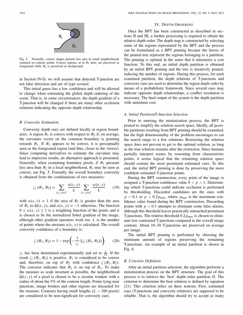
Fig. 5. Normally, convex shapes present less area in small neighborhoodscentered on contour points. Convex regions, as in R1 here, are perceived asforeground while R2 is perceived as background.

in Section IV-D, we will assume that detected T-junction arenot false detection and are of type normal.

This initial guess has a low confidence and will be allowedto change when estimating the global depth ordering of thescene. That is, in some circumstances, the depth gradient of aT-junction will be changed if there are many other occlusionrelations indicating the opposite depth relationship.

B. Convexity Estimation

Convexity depth cues are defined locally at region bound-aries. A region R1 is convex with respect to R2 if, on average,the curvature vector on the common boundary is pointingtowards R1. If R1 appears to be convex, it is perceptuallyseen as the foreground region (and thus, closer to the viewer).Since computing derivatives to estimate the curvature maylead to imprecise results, an alternative approach is presented.Generally, when examining boundary pixels, if R1 presentsless area than R2 in a local neighborhood, R1 may be seen asconvex, see Fig. 5. Formally, the overall boundary convexityis obtained from the combinations of two measures:

ζc (R1, R2) =∑

(x,y)∈�

α(x, y)

L

∑(x,y)∈�

w(x, y)

L(19)

with α(x, y) = 1 if the area of R1 is greater than the areaof R2 in �(x, y), and α(x, y) = −1 otherwise. The function0 ≤ w(x, y) ≤ 1 is a weighting function of the points and itis chosen to be the normalized Sobel gradient of the image,although other gradient operators work too. L is the numberof points where the measure α(x, y) is calculated. The overallconvexity confidence of a boundary is:

ζ (R1, R2) = 1 − exp

(− 1

γc‖ζc (R1, R2)‖

)(20)

γc has been determined experimentally and set to 112 . If the

result ζc (R1, R2) is positive, R1 is considered to be convexand, therefore, on top of R2 with confidence ζ (R1, R2).The converse indicates that R2 is on top of R1. To makethe measure as scale invariant as possible, the neighborhood�(x, y) of a pixel is chosen to be a circular window with aradius of about the 5% of the contour length. Points lying nearjunctions, image borders and other regions are discarded forthe measure. Contours having small lengths (L < 100 pixels)are considered to be non-significant for convexity cues.

IV. DEPTH ORDERING

Once the BPT has been constructed as described in sec-tions II and III, a further processing is required to obtain therelative depth order. The depth map is constructed by selectingsome of the regions represented by the BPT and the processcan be formulated as a BPT pruning because the leaves ofthe pruned tree represent the regions belonging to a partition.The pruning is optimal in the sense that it minimizes a costfunction. To this end, an initial depth partition is obtainedby an initial BPT pruning and the tree is iteratively pruned,reducing the number of regions. During this process, for eachexamined partition, the depth relations of T-junctions andconvexity cues are used to determine the region depth order bymeans of a probabilistic framework. Since several cues mayindicate opposite depth relationships, a conflict resolution isnecessary. The final output of the system is the depth partitionwith minimum cost.

A. Initial Partition/T-Junction Selection

Prior to entering the minimization process, the BPT ispruned to simplify the solution search space. Ideally, all possi-ble partitions resulting from BPT pruning should be examined,but the high dimensionality of the problem encourages to cutthe search range to a few solutions. Restricting the solutionspace does not prevent to get to the optimal solution, as longas the true solution remains after the restriction. Since humanspartially interpret scenes by reasoning from characteristicpoints, it seems logical that the remaining solution spaceshould contain the most prominent estimated cues. To thisend, the initial BPT pruning is done by preserving the moreconfident estimated T-junction points.

During the BPT construction, every point of the image isassigned a T-junction confidence value 0 < p < 1. Determin-ing which T-junctions could indicate occlusion is performedby thresholding. Discarded candidates are the ones withp < 0.1 or p < 0.2 pmax, where pmax is the maximum con-fidence value found during the BPT construction. Discardingpoints with p < 0.1 attempts to eliminate some false alarms,although this threshold leaves practically untouched prominentT-junctions. The relative threshold 0.2 pmax is chosen to elimi-nate low-contrasted T-junctions compared to the overall imagecontrast. About 10–30 T-junctions are preserved on averageper image.

The initial BPT pruning is performed by choosing theminimum amount of regions preserving the remainingT-junctions. An example of an initial partition is shown inFig. 6.

B. Criterion Definition

After an initial partition selection, the algorithm performs aminimization process on the BPT structure. The goal of thisprocess is to retrieve the ’best’ depth order partition D. Thecriterion to determine the best solution is defined by equation(21). This criterion relies on three notions: First, estimatedcues (T-junctions and convexity relations) are supposed to bereliable. That is, the algorithm should try to accept as many


Fig. 6. Original image (left) and the partition generated after T-junctionselection (right). Regions are represented by their mean color.

estimated depth cues as possible. Second, natural images canbe decomposed with few depth planes/regions. Third, regionsare expected to have at least one depth relationship withtheir neighbors. Behind these three intuitions, the followingcriterion for D can be defined:

C(D) =∑i∈R

pi + γN N + γuU (21)

where R is the set of rejected depth cues (T-junctions andconvexity relations) for a particular solution. pi is the confi-dence of a T-junction or the confidence of a convexity relationbetween region boundaries. γN and γu are the weights for Nand U . U refers to the number of isolated regions, that is,regions which do not have any depth relationship with anyother in the final depth image. Finally, N stands for the numberof regions composing the final depth partition.

The value of γu is set rather high to efficiently minimizethe number of isolated regions. In practice, values γU > 2produce good results. The value γN is chosen dependingon the values of the confidences found for T-junction andconvexity cues. Since γN weights the number of regions N ,setting a high value encourages the final solution to have fewregions. If the value is high enough, the system output behaveslike a foreground/background segregation system, separatingthe front-most depth plane from the deeper regions. Usually,pmin < γN < pmax, with pmin and pmax being the minimumand maximum confidences found in the image respectively.γN = pmin throughout the experiments of this paper.

C. Minimization Process

The adopted scheme assumes that the final depth orderedpartition D is the one minimizing the criterion C(D). Seekingfor the global minimum of this criterion starting from theinitial partition alone has proven to be difficult, as C(D) isextremely non-convex, with many local minima. The workin [29] attempts to find a global minimum by searching forthe optimal solution with a RANSAC-style algorithm. Forimages with few T-junctions, the solution found can be nearthe optimal. Nevertheless, since the complexity of [29] isexponential with the number of T-junctions, the process turnedout to be unfeasible for relatively complex images. In thiswork, the BPT is used to explore greedily a subset of solutionsand to minimize the criterion. The approach follows a strategythat gradually prunes the tree until the root node is reached.

The initial pruned tree B0 is obtained by the initialT-junction selection. At each iteration t , for each tree Bt , aset of K feasible solutions Bk

t , k = 1 . . . K , are generated byconsidering all the possible prunings that reduce the number

R23

R22 R1

R21 R19

R20 R11 R15 R9

R18 R17

R16 R7

R23

R22 R1

R21 R19

R20 R11 R15 R9

R18 R17

R3 R4

R23

R22 R1

R21 R19

R20 R11

R18 R17

R3 R4 R16 R7

(a) (b) (c)

R23

R22 R1

R21 R19

R20 R11 R15 R9

R18 R17

R3 R4 R16 R7

Fig. 7. Three allowed prunings of a given BPT. For each pruning, the framedleaf nodes are merged to their parent, reducing the number of BPT nodes byone. All other possible prunings in this BPT reduce the number of leavesby more than one. (a)–(c) Results of the prunings (red, blue, and green) areshown at the bottom.

of leaves in Bt by exactly one. In the example of Fig. 7,three such prunings are possible. Since the leaves of eachpruned BPT define a partition, the depth ordered partition Dk

tis obtained for each Bk

t . With all Dkt available, the next tree

Bt+1 is the tree corresponding to the partition of minimumcost:

Dkmin = arg min

Dki

(C(Dk

1), C(Dk2), . . . , C(Dk

s ))

. (22)

The pruning process is applied successively, obtaining at eachiteration Bt and Dt , t = 1 . . . T . At the final iteration T , thetree has only one leaf and cannot be further pruned. The finaldepth ordered partition is:

Dmin = arg minDk

min

(C(D1

min), C(D2min), . . . , C(DT

min))

. (23)

As can be seen in the previous minimization procedure, adepth ordered partition has to be generated from each prunedtree B . To this end, local depth cues should propagate theirdepth information through regions by means of a Depth OrderGraph (DOG). Since conflicts may appear, a probabilisticscheme to resolve these conflicts is proposed.

D. Probabilistic Framework for Depth Ordering

Since the initially computed cues are merely local, a globalreasoning should be done to arrive at a consistent solution forthe whole image. To this end, a Depth Order Graph (DOG) isconstructed for each partition extracted from the BPT. Nodesin the graph represent regions of the partition extracted fromthe leaves of the BPT. The depth relations are representedin the DOG by directed weighted edges, going from the


foreground region to the background one. There is exactlyone edge going from region R1 to R2 if there is a depth cuei (T-junction or convexity) stating that R1 is in front of R2.The weight of this edge is the cue confidence, pi .

To order the regions according to depth, the DOG shouldbe acyclic (with no conflicts). To achieve such a graphstructure, the DOG has to be modified. To this end, it isinterpreted as a network of reliable links [34]. Each edge in theDOG associated with a cue i is reliable with probability pi .A region R j is reachable from Ri if there exists at least onedirected path that goes from the former region to the latter. Theprobability of existence of this path ρi j is defined as reliabilityin [34], and referred in this work as probability of precedence(PoP) due to its nature. That is, the PoP ρi j is the probabilityof a region Ri to be in the foreground of R j . The proposedsolution to create a direct acyclic graph from the DOG can besummarized as follows:

1) Compute the PoP, ρi j , for every pair of regions (nodes),Ri and R j , that is, the probability that Ri is in theforeground of R j .

2) Examine all pairs ρi j and ρ j i . If a cycle is present,both Ri and R j can be foreground and, therefore, bothρi j , ρ j i �= 0.

3) In case of conflict, modify one of the paths from Ri toR j or vice versa to eliminate the cycle.

The probability ρi j can be calculated exactly by theinclusion–exclusion principle [34]. Nevertheless, its compu-tation cost encourages to find approximate solutions. Sincethe exact value of ρi j is not the ultimate goal of the conflictresolution step, an upper bound proved to give reasonableresults. The PoP is computed using a variant of the Floyd–Warshall algorithm [35]:

for j=1…|V | dofor i=1…|V | do

for k=1…|V | doρn+1

ik = ρnik + ρn

i j ρnjk − ρn

ikρni j ρ

njk

end forend for

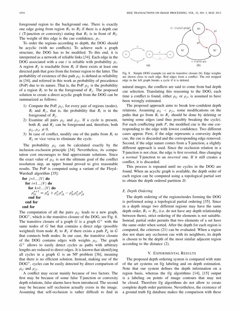
end forThe computation of all the pairs ρi j leads to a new graph,DOG+, which is the transitive closure of the DOG, see Fig. 8.The transitive closure of a graph G is a graph G+ with thesame nodes of G but that contains a direct edge (possiblyweighted) from node Ri to R j if there exists a path Pq in Gthat connects both nodes. In our case, the transitive closureof the DOG contains edges with weights ρi j . The graphG+ allows to easily detect cycles as paths with arbitrarylengths are reduced to direct edges. It is known that identifyingall cycles in a graph G is an NP problem [36], meaningthat there is no efficient solution. Instead, making use of theDOG+, cycles can be easily detected by direct comparison ofρi j and ρ j i .

A conflict may occur mainly because of two factors. Thefirst may be because of some false T-junction or convexitydepth relations, false alarms have been introduced. The secondmay be because self occlusion actually exists in the image.Assuming that self-occlusion is rather difficult to find in

(a) (b)

Fig. 8. Simple DOG example (a) and its transitive closure (b). Edge weightsare shown close to each edge. Red edges form a conflict. The red strippededge in the left graph breaks a cycle if it is deleted.

natural images, the conflicts are said to come from bad depthcue selection. Translating this reasoning to the DOG, eachtime a conflict is found, either ρi j or ρ j i is assumed to havebeen wrongly estimated.

The proposed approach aims to break low-confident depthrelations. Assuming ρi j < ρ j i , some modifications on thepaths that go from Ri to R j should be done by deleting orturning some edges (and thus possibly breaking the cycle).For each conflicting path P , the modified cue is the one cor-responding to the edge with lowest confidence. Two differentcases appear. First, if the edge represents a convexity depthcue, the cue is discarded and the corresponding edge removed.Second, if the edge nature comes from a T-junction, a slightlydifferent approach is used. Since the occlusion relation in aT-junction is not clear, the edge is first reverted, thus changinga normal T-junction to an inverted one. If it still creates aconflict, it is discarded.

This process is repeated until no cycles in the DOG arefound. When an acyclic graph is available, the depth order ofeach region can be computed using a topological partial sortto obtain the depth ordered partition D.

E. Depth Ordering

The depth ordering of the regions/nodes forming the DOGis performed using a topological partial ordering [35]. Sincein a depth image two different regions may have the samedepth order, R1 = R2, (i.e. do not have any depth relationshipbetween them), strict ordering of the elements is not suitable.Instead, partial order permits that two elements of a set havethe same order when sorted. After the depth for each region iscomputed, the criterion (21) can be evaluated. When a regiondoe not share any occlusion cue with its neighbors, its depthis chosen to be the depth of the most similar adjacent regionaccording to the distance (2).

V. EXPERIMENTAL RESULTS

The proposed depth ordering system is compared with stateof the art systems on f/g labeling and on depth estimation.Note that our system defines the depth information on aregion basis, whereas the f/g algorithms [14], [15] outputis a labeling on points of image contours that may notbe closed. Therefore f/g algorithms do not allow to createcomplete depth order partitions. Nevertheless, the existence ofa ground truth f/g database makes the comparison with these


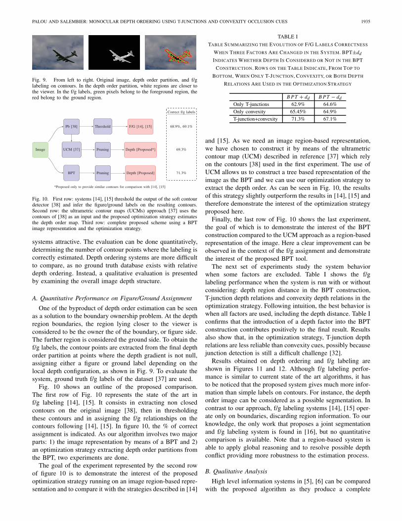
Fig. 9. From left to right. Original image, depth order partition, and f/glabeling on contours. In the depth order partition, white regions are closer tothe viewer. In the f/g labels, green pixels belong to the foreground region, thered belong to the ground region.

Fig. 10. First row: systems [14], [15] threshold the output of the soft contourdetector [38] and infer the figure/ground labels on the resulting contours.Second row: the ultrametric contour maps (UCMs) approach [37] uses thecontours of [38] as an input and the proposed optimization strategy estimatesthe depth order map. Third row: complete proposed scheme using a BPTimage representation and the optimization strategy.

systems attractive. The evaluation can be done quantitatively,determining the number of contour points where the labeling iscorrectly estimated. Depth ordering systems are more difficultto compare, as no ground truth database exists with relativedepth ordering. Instead, a qualitative evaluation is presentedby examining the overall image depth structure.

A. Quantitative Performance on Figure/Ground Assignment

One of the byproduct of depth order estimation can be seenas a solution to the boundary ownership problem. At the depthregion boundaries, the region lying closer to the viewer isconsidered to be the owner the of the boundary, or figure side.The further region is considered the ground side. To obtain thef/g labels, the contour points are extracted from the final depthorder partition at points where the depth gradient is not null,assigning either a figure or ground label depending on thelocal depth configuration, as shown in Fig. 9. To evaluate thesystem, ground truth f/g labels of the dataset [37] are used.

Fig. 10 shows an outline of the proposed comparison.The first row of Fig. 10 represents the state of the art inf/g labeling [14], [15]. It consists in extracting non closedcontours on the original image [38], then in thresholdingthese contours and in assigning the f/g relationships on thecontours following [14], [15]. In figure 10, the % of correctassignment is indicated. As our algorithm involves two majorparts: 1) the image representation by means of a BPT and 2)an optimization strategy extracting depth order partitions fromthe BPT, two experiments are done.

The goal of the experiment represented by the second rowof figure 10 is to demonstrate the interest of the proposedoptimization strategy running on an image region-based repre-sentation and to compare it with the strategies described in [14]

TABLE I

TABLE SUMMARIZING THE EVOLUTION OF F/G LABELS CORRECTNESS

WHEN THREE FACTORS ARE CHANGED IN THE SYSTEM. BPT±dd

INDICATES WHETHER DEPTH IS CONSIDERED OR NOT IN THE BPT

CONSTRUCTION. ROWS ON THE TABLE INDICATE, FROM TOP TO

BOTTOM, WHEN ONLY T-JUNCTION, CONVEXITY, OR BOTH DEPTH

RELATIONS ARE USED IN THE OPTIMIZATION STRATEGY

B PT + dd B PT − dd

Only T-junctions 62.9% 64.6%

Only convexity 65.45% 64.9%

T-junction+convexity 71.3% 67.1%

and [15]. As we need an image region-based representation,we have chosen to construct it by means of the ultrametriccontour map (UCM) described in reference [37] which relyon the contours [38] used in the first experiment. The use ofUCM allows us to construct a tree based representation of theimage as the BPT and we can use our optimization strategy toextract the depth order. As can be seen in Fig. 10, the resultsof this strategy slightly outperform the results in [14], [15] andtherefore demonstrate the interest of the optimization strategyproposed here.

Finally, the last row of Fig. 10 shows the last experiment,the goal of which is to demonstrate the interest of the BPTconstruction compared to the UCM approach as a region-basedrepresentation of the image. Here a clear improvement can beobserved in the context of the f/g assignment and demonstratethe interest of the proposed BPT tool.

The next set of experiments study the system behaviorwhen some factors are excluded. Table I shows the f/glabeling performance when the system is run with or withoutconsidering: depth region distance in the BPT construction,T-junction depth relations and convexity depth relations in theoptimization strategy. Following intuition, the best behavior iswhen all factors are used, including the depth distance. Table Iconfirms that the introduction of a depth factor into the BPTconstruction contributes positively to the final result. Resultsalso show that, in the optimization strategy, T-junction depthrelations are less reliable than convexity cues, possibly becausejunction detection is still a difficult challenge [32].

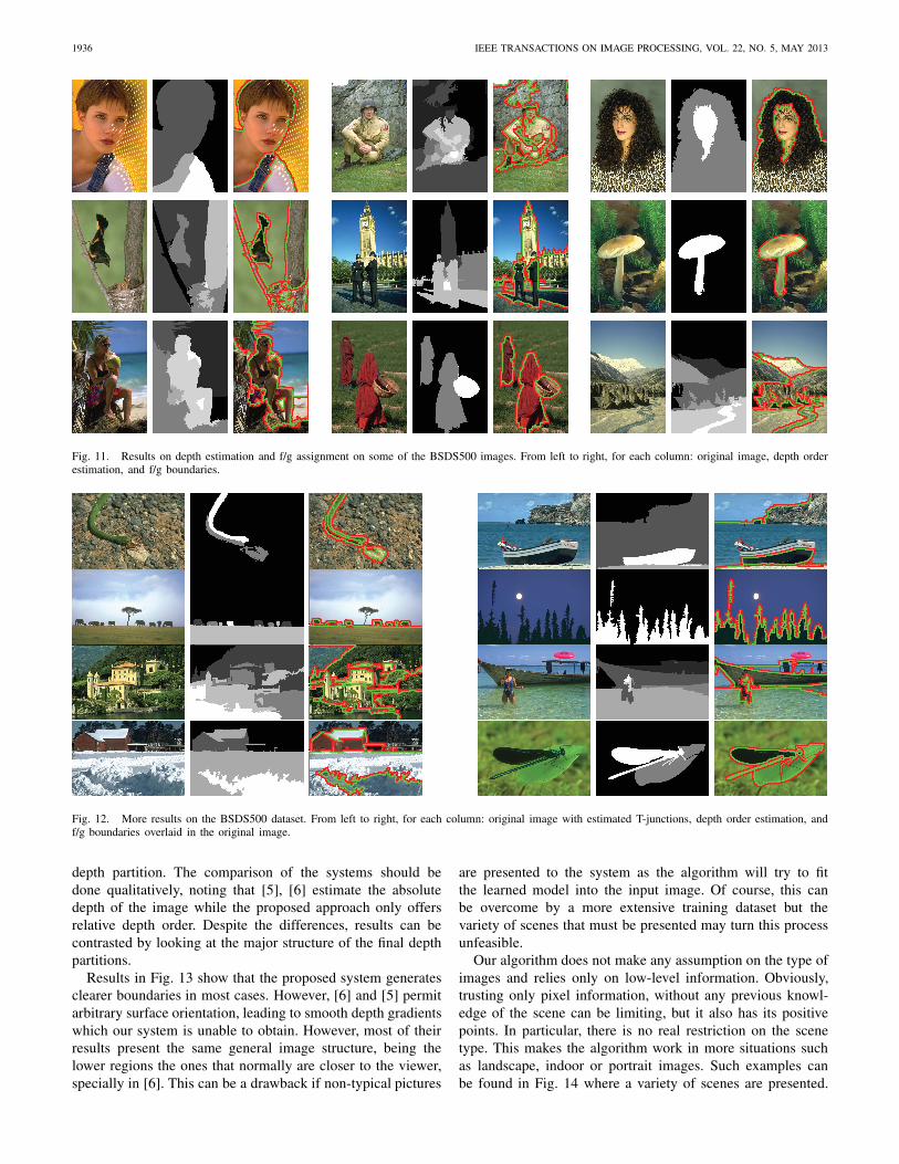
Results obtained on depth ordering and f/g labeling areshown in Figures 11 and 12. Although f/g labeling perfor-mance is similar to current state of the art algorithms, it hasto be noticed that the proposed system gives much more infor-mation than simple labels on contours. For instance, the depthorder image can be considered as a possible segmentation. Incontrast to our approach, f/g labeling systems [14], [15] oper-ate only on boundaries, discarding region information. To ourknowledge, the only work that proposes a joint segmentationand f/g labeling system is found in [16], but no quantitativecomparison is available. Note that a region-based system isable to apply global reasoning and to resolve possible depthconflict providing more robustness to the estimation process.

B. Qualitative Analysis

High level information systems in [5], [6] can be comparedwith the proposed algorithm as they produce a complete


Fig. 11. Results on depth estimation and f/g assignment on some of the BSDS500 images. From left to right, for each column: original image, depth orderestimation, and f/g boundaries.

Fig. 12. More results on the BSDS500 dataset. From left to right, for each column: original image with estimated T-junctions, depth order estimation, andf/g boundaries overlaid in the original image.

depth partition. The comparison of the systems should bedone qualitatively, noting that [5], [6] estimate the absolutedepth of the image while the proposed approach only offersrelative depth order. Despite the differences, results can becontrasted by looking at the major structure of the final depthpartitions.

Results in Fig. 13 show that the proposed system generatesclearer boundaries in most cases. However, [6] and [5] permitarbitrary surface orientation, leading to smooth depth gradientswhich our system is unable to obtain. However, most of theirresults present the same general image structure, being thelower regions the ones that normally are closer to the viewer,specially in [6]. This can be a drawback if non-typical pictures

are presented to the system as the algorithm will try to fitthe learned model into the input image. Of course, this canbe overcome by a more extensive training dataset but thevariety of scenes that must be presented may turn this processunfeasible.

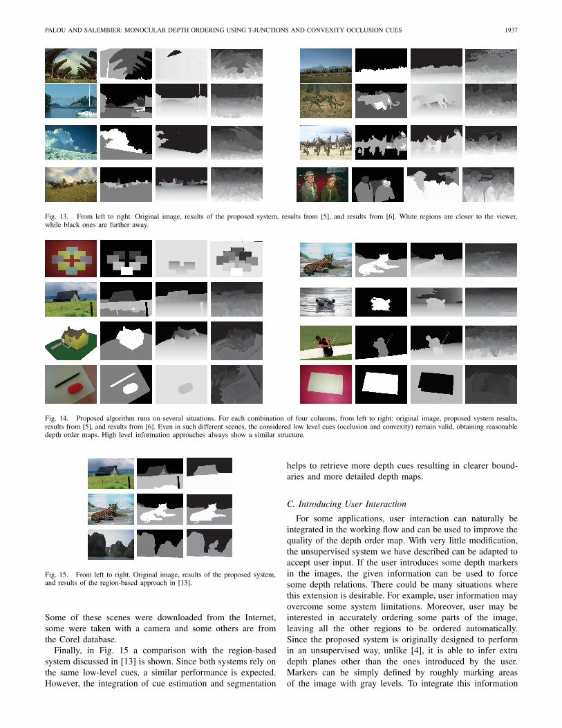
Our algorithm does not make any assumption on the type ofimages and relies only on low-level information. Obviously,trusting only pixel information, without any previous knowl-edge of the scene can be limiting, but it also has its positivepoints. In particular, there is no real restriction on the scenetype. This makes the algorithm work in more situations suchas landscape, indoor or portrait images. Such examples canbe found in Fig. 14 where a variety of scenes are presented.


Fig. 13. From left to right. Original image, results of the proposed system, results from [5], and results from [6]. White regions are closer to the viewer,while black ones are further away.

Fig. 14. Proposed algorithm runs on several situations. For each combination of four columns, from left to right: original image, proposed system results,results from [5], and results from [6]. Even in such different scenes, the considered low level cues (occlusion and convexity) remain valid, obtaining reasonabledepth order maps. High level information approaches always show a similar structure.

Fig. 15. From left to right. Original image, results of the proposed system,and results of the region-based approach in [13].

Some of these scenes were downloaded from the Internet,some were taken with a camera and some others are fromthe Corel database.

Finally, in Fig. 15 a comparison with the region-basedsystem discussed in [13] is shown. Since both systems rely onthe same low-level cues, a similar performance is expected.However, the integration of cue estimation and segmentation

helps to retrieve more depth cues resulting in clearer bound-aries and more detailed depth maps.

C. Introducing User Interaction

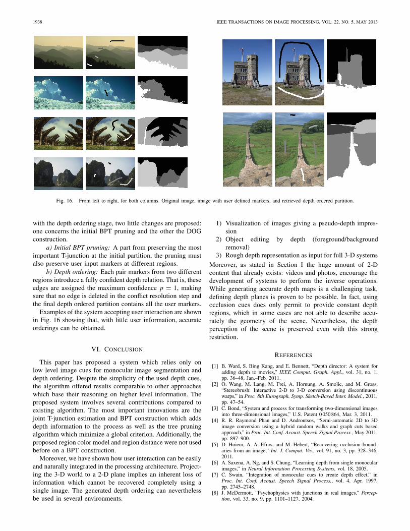
For some applications, user interaction can naturally beintegrated in the working flow and can be used to improve thequality of the depth order map. With very little modification,the unsupervised system we have described can be adapted toaccept user input. If the user introduces some depth markersin the images, the given information can be used to forcesome depth relations. There could be many situations wherethis extension is desirable. For example, user information mayovercome some system limitations. Moreover, user may beinterested in accurately ordering some parts of the image,leaving all the other regions to be ordered automatically.Since the proposed system is originally designed to performin an unsupervised way, unlike [4], it is able to infer extradepth planes other than the ones introduced by the user.Markers can be simply defined by roughly marking areasof the image with gray levels. To integrate this information


Fig. 16. From left to right, for both columns. Original image, image with user defined markers, and retrieved depth ordered partition.

with the depth ordering stage, two little changes are proposed:one concerns the initial BPT pruning and the other the DOGconstruction.

a) Initial BPT pruning: A part from preserving the mostimportant T-junction at the initial partition, the pruning mustalso preserve user input markers at different regions.

b) Depth ordering: Each pair markers from two differentregions introduce a fully confident depth relation. That is, theseedges are assigned the maximum confidence p = 1, makingsure that no edge is deleted in the conflict resolution step andthe final depth ordered partition contains all the user markers.

Examples of the system accepting user interaction are shownin Fig. 16 showing that, with little user information, accurateorderings can be obtained.

VI. CONCLUSION

This paper has proposed a system which relies only onlow level image cues for monocular image segmentation anddepth ordering. Despite the simplicity of the used depth cues,the algorithm offered results comparable to other approacheswhich base their reasoning on higher level information. Theproposed system involves several contributions compared toexisting algorithm. The most important innovations are thejoint T-junction estimation and BPT construction which addsdepth information to the process as well as the tree pruningalgorithm which minimize a global criterion. Additionally, theproposed region color model and region distance were not usedbefore on a BPT construction.

Moreover, we have shown how user interaction can be easilyand naturally integrated in the processing architecture. Project-ing the 3-D world to a 2-D plane implies an inherent loss ofinformation which cannot be recovered completely using asingle image. The generated depth ordering can neverthelessbe used in several environments.

1) Visualization of images giving a pseudo-depth impres-sion

2) Object editing by depth (foreground/backgroundremoval)

3) Rough depth representation as input for full 3-D systems

Moreover, as stated in Section I the huge amount of 2-Dcontent that already exists: videos and photos, encourage thedevelopment of systems to perform the inverse operations.While generating accurate depth maps is a challenging task,defining depth planes is proven to be possible. In fact, usingocclusion cues does only permit to provide constant depthregions, which in some cases are not able to describe accu-rately the geometry of the scene. Nevertheless, the depthperception of the scene is preserved even with this strongrestriction.

REFERENCES

[1] B. Ward, S. Bing Kang, and E. Bennett, “Depth director: A system foradding depth to movies,” IEEE Comput. Graph. Appl., vol. 31, no. 1,pp. 36–48, Jan.–Feb. 2011.

[2] O. Wang, M. Lang, M. Frei, A. Hornung, A. Smolic, and M. Gross,“Stereobrush: Interactive 2-D to 3-D conversion using discontinuouswarps,” in Proc. 8th Eurograph. Symp. Sketch-Based Inter. Model., 2011,pp. 47–54.

[3] C. Bond, “System and process for transforming two-dimensional imagesinto three-dimensional images,” U.S. Patent 0 050 864, Mar. 3, 2011.

[4] R. R. Raymond Phan and D. Androutsos, “Semi-automatic 2D to 3Dimage conversion using a hybrid random walks and graph cuts basedapproach,” in Proc. Int. Conf. Acoust. Speech Signal Process., May 2011,pp. 897–900.

[5] D. Hoiem, A. A. Efros, and M. Hebert, “Recovering occlusion bound-aries from an image,” Int. J. Comput. Vis., vol. 91, no. 3, pp. 328–346,2011.

[6] A. Saxena, A. Ng, and S. Chung, “Learning depth from single monocularimages,” in Neural Information Processing Systems, vol. 18, 2005.

[7] C. Swain, “Integration of monocular cues to create depth effect,” inProc. Int. Conf. Acoust. Speech Signal Process., vol. 4. Apr. 1997,pp. 2745–2748.

[8] J. McDermott, “Psychophysics with junctions in real images,” Percep-tion, vol. 33, no. 9, pp. 1101–1127, 2004.


[9] J. Cutrona and N. Bonnet, “Two methods for semi-automatic imagesegmentation based on fuzzy connectedness and watersheds,” in Proc.Int. Conf. Visualizat., Imag. Image Process., Sep. 2001, pp. 1–5.

[10] A. Criminisi, P. Perez, and K. Toyama, “Region filling and objectremoval by exemplar-based image inpainting,” IEEE Trans. ImageProcess., vol. 13, no. 9, pp. 1200–1212, Sep. 2004.

[11] A. Criminisi, I. Reid, and A. Zisserman, “Single view metrology,” inProc. 7th IEEE Int. Conf. Comput. Vis., vol. 1. Sep. 1999, pp. 434–441.

[12] A. Torralba and A. Oliva, “Depth estimation from image structure,”IEEE Trans. Pattern Anal. Mach. Intell., vol. 24, no. 9, pp. 1226–1238,Sep. 2002.

[13] M. Dimiccoli, “Monocular depth estimation for image segmentationand filtering,” Dept. Signal Theory Commun., Ph.D. dissertation, Univ.Politecnica de Catalunya, Barcelona, Spain, 2009.

[14] X. Ren, C. Fowlkes, and J. Malik, “Figure/ground assignment in naturalimages,” in Proc. Eur. Conf. Comput. Vis., 2006, pp. 614–627.

[15] I. Leichter and M. Lindenbaum, “Boundary ownership by lifting to2.1d,” in Proc. IEEE Int. Conf. Comput. Vis., Sep.–Oct. 2009, pp. 9–16.

[16] M. Maire, “Simultaneous segmentation and figure/ground organizationusing angular embedding,” in Proc. Eur. Conf. Comput. Vis., 2010,pp. 450–464.

[17] D. Marr, Vision: A Computational Investigation into the Human Rep-resentation and Processing of Visual Information. San Francisco, CA,USA: W.H. Freeman, 1982.

[18] S. H. Schwartz, Visual Perception: A Clinical Orientation, 3rd ed. NewYork, USA: McGraw-Hill, May 2004.

[19] S. M. Smith and J. M. Brady, “Susan-a new approach to low level imageprocessing,” Int. J. Comput. Vis., vol. 23, pp. 45–78, May 1997.

[20] P. Salembier and L. Garrido, “Binary partition tree as an efficientrepresentation for image processing, segmentation, and informationretrieval,” IEEE Trans. Image Process., vol. 9, no. 4, pp. 561–576, Apr.2000.

[21] V. Vilaplana, F. Marques, and P. Salembier, “Binary partition treesfor object detection,” IEEE Trans. Image Process., vol. 17, no. 11,pp. 2201–2216, Nov. 2008.

[22] M. A. Ruzon and C. Tomasi, “Edge, junction, and corner detection usingcolor distributions,” IEEE Trans. Pattern Anal. Mach. Intell., vol. 23,no. 11, pp. 1281–1295, Nov. 2001.

[23] F. Calderero and F. Marques, “Region merging techniques using infor-mation theory statistical measures,” IEEE Trans. Image Process., vol. 19,no. 6, pp. 1567–1586, Jun. 2010.

[24] B. S. Manjunath, J. R. Ohm, V. V. Vasudevan, and A. Yamada, “Colorand texture descriptors,” IEEE Trans. Circuits Syst. Video Technol.,vol. 11, no. 6, pp. 703–715, Jan. 1998.

[25] M. Orchard and C. Bouman, “Color quantization of images,” IEEETrans. Signal Process., vol. 39, no. 12, pp. 2677–2690, Dec. 1991.

[26] R. N. Shepard, “Toward a universal law of generalization for psycho-logical science,” Science, vol. 237, no. 4820, pp. 1317–1323, 1987.

[27] Y. Rubner, C. Tomasi, and L. Guibas, “A metric for distributions withapplications to image databases,” in Proc. 6th Int. Conf. Comput. Vis.,Jan. 1998, pp. 59–66.

[28] F. Hillier and G. Lieberman, Introduction to Mathematical Program-ming. New York, USA: McGraw-Hill, 1990.

[29] G. Palou and P. Salembier, “Occlusion-based depth ordering on monoc-ular images with binary partition tree,” in Proc. IEEE Int. Conf. Acoust.,Speech Signal Process., May 2011, pp. 1093–1096.

[30] R. Bergevin and A. Bubel, “Detection and characterization of junctionsin a 2D image,” Comput. Vis. Image Understand., vol. 93, no. 3,pp. 288–309, 2004.

[31] C. Harris and M. Stephens, “A combined corner and edge detection,” inProc. 4th Alvey Vis. Conf., 1988, pp. 147–151.

[32] M. Maire, P. Arbelaez, C. Fowlkes, and J. Malik, “Using contours todetect and localize junctions in natural images,” in Proc. IEEE Conf.Comput. Vis. Pattern Recognit., Jun. 2008, pp. 1–8.

[33] F. Guichard, L. Moisan, and J.-M. Morel, A review of P.D.E. models inimage processing and image analysis,” J. Phys. IV, vol. 12, no. 1, pp.137–154, Mar. 2002.

[34] R. Terruggia, “Reliability analysis of probabilistic networks,” Ph.D.dissertation, Dept. Comput. Sci., Univ. degli Studi di Torino, Turin, Italy,2010.

[35] T. H. Cormen, C. E. Leiserson, R. L. Rivest, and C. Stein, IntroductionAlgorithms, 2nd ed. Cambridge, MA, USA: MIT Press, Sep. 2001.

[36] P. Mateti and N. Deo, “On algorithms for enumerating all circuits of agraph,” J. Comput. Soc. Ind. Appl. Math., vol. 5, no. 1, pp. 90–99, 1976.

[37] P. Arbelaez, M. Maire, C. Fowlkes, and J. Malik, “Contour detectionand hierarchical image segmentation,” EECS Dept, Univ. California,Berkeley, USA, Tech. Rep. UCB/EECS-2010-17, Feb. 2010.

[38] D. Martin, C. Fowlkes, and J. Malik, “Learning to detect natural imageboundaries using local brightness, color, and texture cues,” IEEE Trans.Pattern Anal. Mach. Intell., vol. 26, no. 5, pp. 530–549, May 2004.

Guillem Palou (S’11) received the degree in elec-trical engineering from the Technical University ofCatalonia (UPC), Barcelona, Spain, and the finaldegree from the Massachusetts Institute of Technol-ogy, Boston, MA, USA, both in 2009. He is currentlypursuing the Ph.D. degree with the Image ProcessingGroup, UPC.

His current research interests include monoculardepth perception, image segmentation, and featuredetection.

Mr. Palou was a recipient of a Scholarship fromthe Generalitat de Catalunya.

Philippe Salembier (M’96–SM’09–F’12) receivedthe degree from the École Polytechnique, Paris,France, and the degree from the École NationaleSupérieure des Télécommunications, Paris, in 1983and 1985, respectively, and the Ph.D. degree fromthe Swiss Federal Institute of Technology (EPFL),Lausanne, Switzerland, in 1991.

He was a Post-Doctoral Fellow with the Har-vard Robotics Laboratory, Cambridge, MA, USA,in 1991. From 1985 to 1989, he was with the Lab-oratoires d’Electronique Philips, Limeil-Brevannes,

France, where he was involved in research on digital communications andsignal processing for HDTV. In 1989, he joined the Signal ProcessingLaboratory, EPFL, where he was engaged in research on image processing.In 1991, he was with the Harvard Robotics Laboratory and then with theTechnical University of Catalonia, Barcelona, Spain, where he is currently aProfessor of digital signal and image processing. His current research interestsinclude image and sequence coding, compression and indexing, segmentation,video sequence analysis, mathematical morphology, level sets, and nonlinearfiltering.

Dr. Salembier was an Area Editor of the Journal of Visual Commu-nication and Image Representation (Academic Press) from 1995 to 1998and an AdCom Officer of the European Association for Signal Processing(EURASIP) from 1994 to 1999. He was a Guest Editor of special issuesof Signal Processing on mathematical morphology in 1994 and on videosequence analysis in 1998. He was a Co-Editor of a special issue of SignalProcessing: Image Communication on MPEG-7 Technology in 2000. He wasthe Co-Editor-In-Chief of Signal Processing from 2001 to 2002. He was amember on the Image and Multidimensional Signal Processing TechnicalCommittee of the IEEE Signal Processing Society from 2000 to 2006 andwas the Technical Chair of the IEEE International Conference on ImageProcessing 2003 in Barcelona. He was an Associate Editor of the IEEETRANSACTIONS ON IMAGE PROCESSING from 2002 to 2008 and the IEEESignal Processing Letters from 2005 to 2008. He is currently an AssociateEditor of the EURASIP Journal on Image and Video Processing, SignalProcessing: Image Communication (Elsevier), and the IEEE TRANSACTIONS

ON CIRCUITS AND SYSTEMS FOR VIDEO TECHNOLOGY. He was involvedin the definition of the MPEG-7 standard (Multimedia Content DescriptionInterface) as the Chair of the Multimedia Description Scheme Group from1999 to 2001.

Monocular Depth Ordering Using T-Junctions and Convexity Occlusion Cues

Documents