Monitoring Numerical Stability of Coupled MC codes …montecarlo.vtt.fi/mtg/2013_Berkeley/Dan_Kotlyar2.pdfMonitoring Numerical Stability of Coupled MC codes Serpent User's group meeting,

1

Monitoring Numerical Stability of

Coupled MC codes

Serpent User's group meeting, Berkeley, CA,

November 6-8, 2013

D. Kotlyar, E. Shwageraus

Department of Nuclear Engineering,

Ben Gurion University of the Negev

2

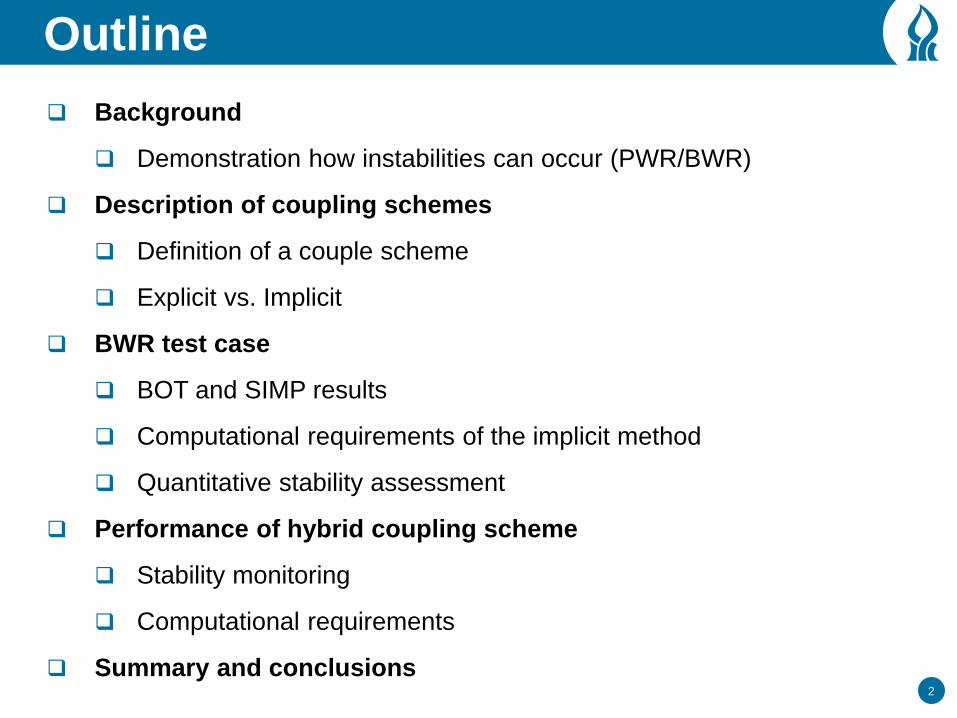
Outline

Background

Demonstration how instabilities can occur (PWR/BWR)

Description of coupling schemes

Definition of a couple scheme

Explicit vs. Implicit

BWR test case

BOT and SIMP results

Computational requirements of the implicit method

Quantitative stability assessment

Performance of hybrid coupling scheme

Stability monitoring

Computational requirements

Summary and conclusions

3

MC-Burnup-Thermal hydraulic coupling

The objective of the coupled MC analysis is to obtain:

Nuclide density field as a function of t

TH properties as a function of t

This non-linear problem is solved by operator splitting

Described by 3 coupled equations:

Burnup: describes the changes in ND

Heat balance equation: computes temperature distribution

Eigenvalue neutron transport equation: provides the neutron flux

How to couple the independent solutions ?

4

Explicit vs. Implicit methods

The explicit BOT method

Neutronic-TH convergence at BOS

Depletion with BOS (explicit) flux values

May be unstable due to the numerical explicit coupling scheme

Stochastic Implicit Mid-Point (SIMP) method

Simultaneous convergence of ND and TH fields

Uses EOS fluxes and thus implicit

Flux/power/temperatures are time-step averaged quantities

Proven to be numerically stable

5

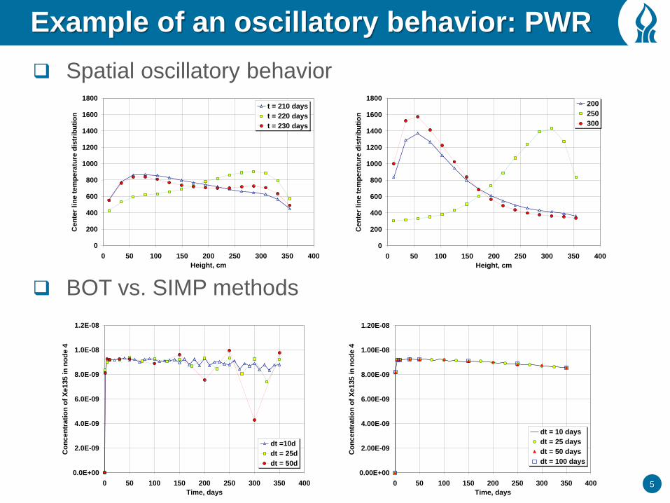
Example of an oscillatory behavior: PWR

Spatial oscillatory behavior

BOT vs. SIMP methods

0

200

400

600

800

1000

1200

1400

1600

1800

0 50 100 150 200 250 300 350 400

Height, cm

Ce

nte

r li

ne t

em

pe

ratu

re d

istr

ibu

tio

n

200

250

300

0.0E+00

2.0E-09

4.0E-09

6.0E-09

8.0E-09

1.0E-08

1.2E-08

0 50 100 150 200 250 300 350 400

Time, days

Co

ncen

trati

on

of

Xe135 in

no

de 4

dt =10d

dt = 25d

dt = 50d

0.00E+00

2.00E-09

4.00E-09

6.00E-09

8.00E-09

1.00E-08

1.20E-08

0 50 100 150 200 250 300 350 400

Time, days

Co

nc

en

tra

tio

n o

f X

e1

35

in

no

de 4

dt = 10 days

dt = 25 days

dt = 50 days

dt = 100 days

0

200

400

600

800

1000

1200

1400

1600

1800

0 50 100 150 200 250 300 350 400

Height, cm

Cen

ter

lin

e t

em

pera

ture

dis

trib

uti

on

t = 210 days

t = 220 days

t = 230 days

6

Test Case Description

77 BWR assembly, UO2 fuel

36 axial burnup regions

Previous work examined PWR assembly

The oscillations developed immediately (BOL)

Axial void dist. determines the flux dist. @ BOL

Initially, local burnup effects do not affect the flux shape

Numerical oscillations can still develop at higher burnup

Void dist. effect is compensated by the burnup dist. effect

7

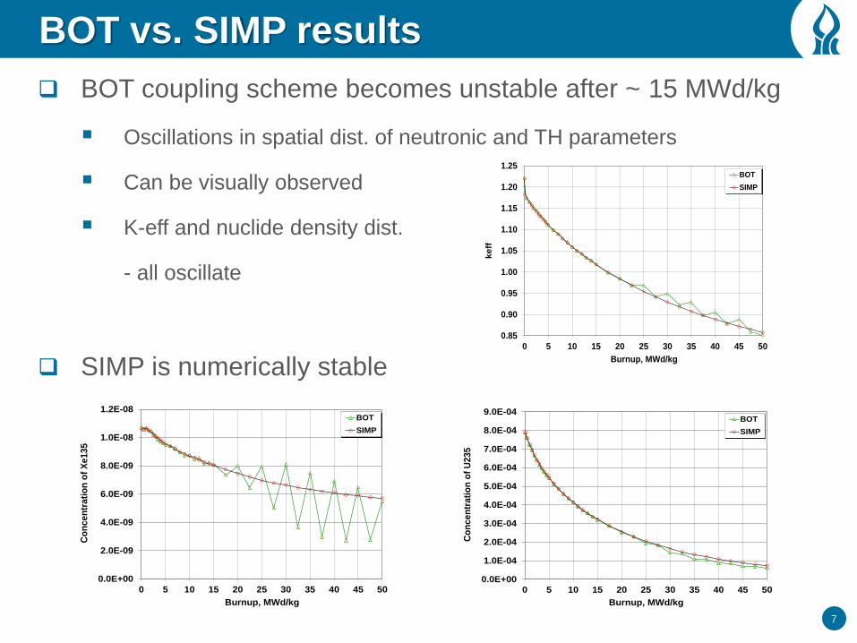
BOT vs. SIMP results

BOT coupling scheme becomes unstable after ~ 15 MWd/kg

Oscillations in spatial dist. of neutronic and TH parameters

Can be visually observed

K-eff and nuclide density dist.

- all oscillate

SIMP is numerically stable

0.85

0.90

0.95

1.00

1.05

1.10

1.15

1.20

1.25

0 5 10 15 20 25 30 35 40 45 50

ke

ff

Burnup, MWd/kg

BOT

SIMP

0.0E+00

2.0E-09

4.0E-09

6.0E-09

8.0E-09

1.0E-08

1.2E-08

0 5 10 15 20 25 30 35 40 45 50

Co

ncen

tra

tio

n o

f X

e13

5

Burnup, MWd/kg

BOT

SIMP

0.0E+00

1.0E-04

2.0E-04

3.0E-04

4.0E-04

5.0E-04

6.0E-04

7.0E-04

8.0E-04

9.0E-04

0 5 10 15 20 25 30 35 40 45 50

Co

ncen

tra

tio

n o

f U

23

5

Burnup, MWd/kg

BOT

SIMP

8

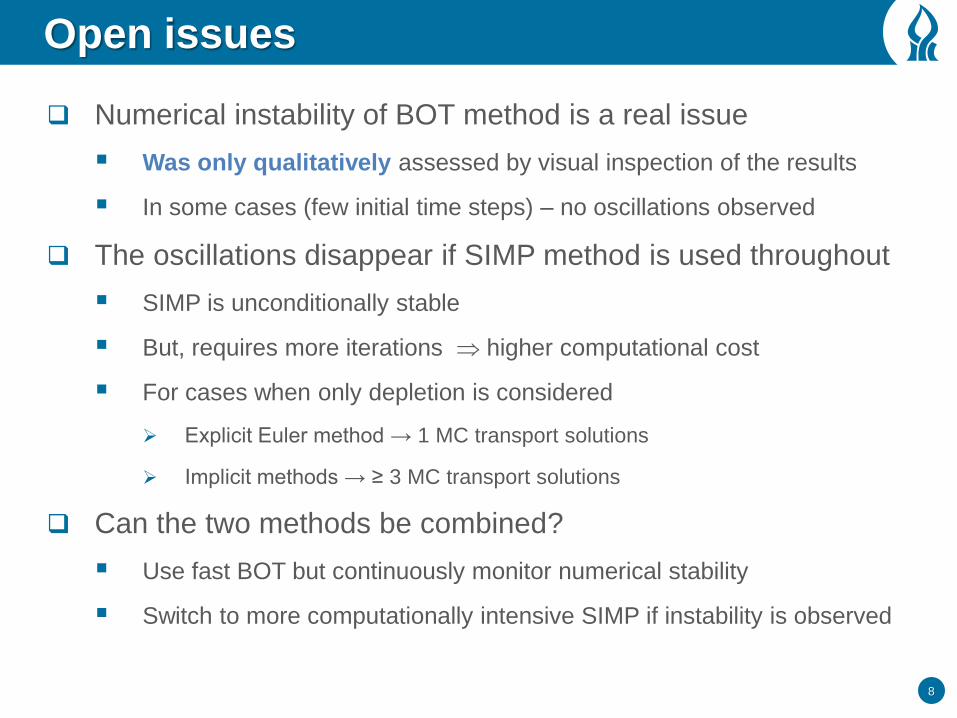
Open issues

Numerical instability of BOT method is a real issue

Was only qualitatively assessed by visual inspection of the results

In some cases (few initial time steps) – no oscillations observed

The oscillations disappear if SIMP method is used throughout

SIMP is unconditionally stable

But, requires more iterations higher computational cost

For cases when only depletion is considered

Explicit Euler method → 1 MC transport solutions

Implicit methods → ≥ 3 MC transport solutions

Can the two methods be combined?

Use fast BOT but continuously monitor numerical stability

Switch to more computationally intensive SIMP if instability is observed

9

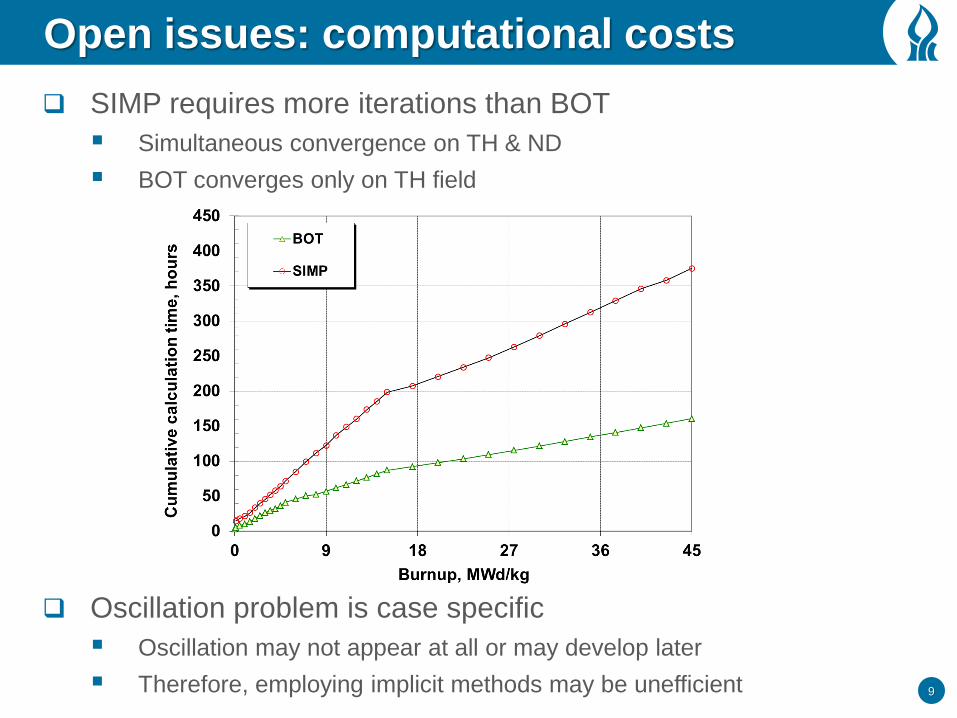
Open issues: computational costs

SIMP requires more iterations than BOT

Simultaneous convergence on TH & ND

BOT converges only on TH field

Oscillation problem is case specific

Oscillation may not appear at all or may develop later

Therefore, employing implicit methods may be unefficient

10

Alternative solution approach

Diagnostic mechanism is required:

To identify the onset of numerical instabilities,

To alert the user, or

Automatically switch to SIMP algorithm

BOT (fast and simple) → SIMP unconditionally stable but

computationally more expensive

Such hybrid algorithm was developed and implemented in BGCore

Assures numerical stability

Improves computational efficiency of coupled MC codes

Does not require any intervention from the user

11

The irradiation time is subdivided into time steps

At each time-step

Iteratively solve MC, depletion and TH problems

The procedure is repeated for the following steps

The global solution at any base point n is achieved by:

Sequentially solving the prior sub-steps (≤ n)

Analyzing the behavior of time integration method

Define amplification (growth) factor: G

The solution is stable if G is bounded

Keep monitoring G for the following steps

Depletion calculations

⋯

n

Time

0 1 2

⋯

i

12

Stability of numerical schemes

A stable scheme produces a bounded solution if the exact

solution is bounded

Error between computed solution and the exact solution

should not be amplified as we progress in time

Notation:

𝑈 𝑁 Exact solution

𝑈𝑁 Computed solution

𝜀𝑁 error = 𝑈 𝑁- 𝑈𝑁

The stability requires that:

𝐺 =𝑁+1

𝑁 ≤ 1

The growth factor must satisfy this condition for all time-steps

13

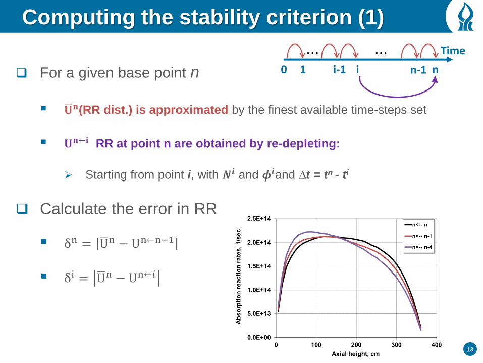
Computing the stability criterion (1)

For a given base point n

𝐔 𝐧(RR dist.) is approximated by the finest available time-steps set

𝐔𝐧←𝐢 RR at point n are obtained by re-depleting:

Starting from point i, with 𝑵𝒊 and 𝝓𝒊and ∆t = tn - ti

Calculate the error in RR

δn = U n − Un←n−1

δi = U n − Un←𝑖

n

Time

0 1 i-1

⋯ i

⋯ n-1

14

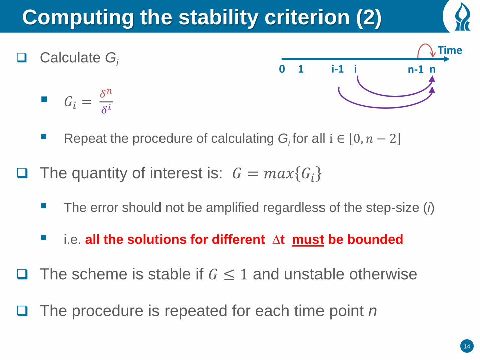
Computing the stability criterion (2)

Calculate Gi

𝐺𝑖 = 𝛿𝑛

𝛿𝑖

Repeat the procedure of calculating Gi for all i ∈ 0, 𝑛 − 2

The quantity of interest is: 𝐺 = 𝑚𝑎𝑥 𝐺𝑖

The error should not be amplified regardless of the step-size (i)

i.e. all the solutions for different ∆t must be bounded

The scheme is stable if 𝐺 ≤ 1 and unstable otherwise

The procedure is repeated for each time point n

n

Time

0 1 i-1 i n-1

15

Results: amplification factor G

Quantitative assessment of the stability

SIMP is stable (G<1)

BOT is stable only up until ~15 MWd/kg

0

4

8

12

16

20

0 9 18 27 36 45

Am

plifi

ca

tio

n f

ac

tor

G

Burnup, MWd/kg

BOT

SIMP

unstable region

stable region

16

Computational efficiency

Total (cumulative) execution time until the onset of oscillations:

BOT 87 hr. (135 transport solutions)

SIMP 198 hr. (278 transport solutions)

Applying BOT (<15 MWd/kg) and SIMP thereafter saves:

111 hr. (143 transport solutions)

CPU costs for calculating G

Loading XS data

Solving Bateman equations

Matrix-Vector multiplication

17

Conclusions (1)

Existing MC coupling methods may be unstable

Stochastic implicit mid-point (SIMP) methods was developed

Unconditionally stable

But, more computationally intensive

Some problems do not have stability issues

Always using SIMP would be a waste of computing resources

18

Conclusions (2)

A method for monitoring numerical stability was developed

Evaluates error amplification factor which must be bounded

Capable of identifying the onset of instability

Can automatically trigger the transition:

From: Explicit BOT

To: Implicit SIMP method

The hybrid method is more computationally efficient

Computational requirements for monitoring stability are negligible

19

Thank you for your attention

20

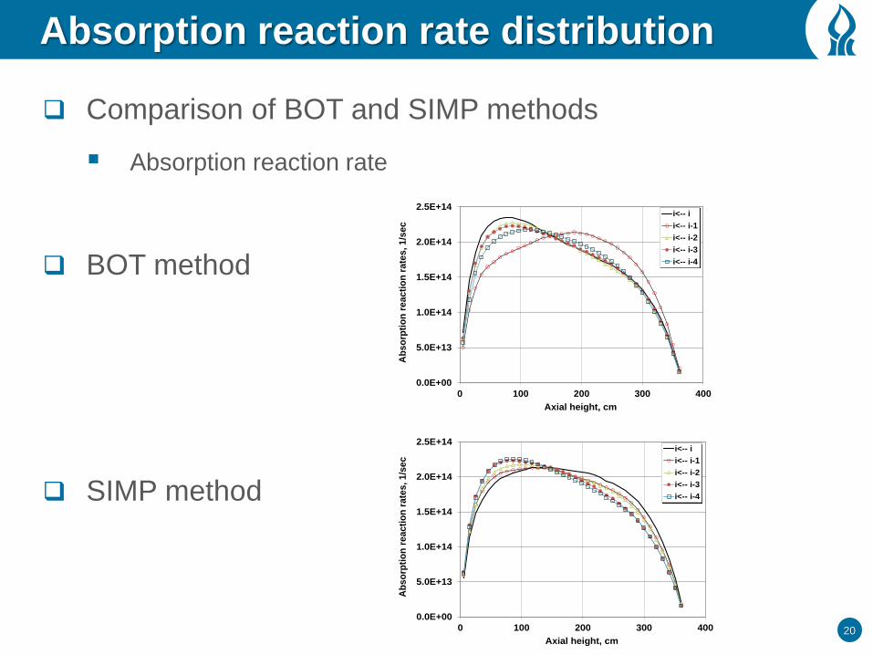
Absorption reaction rate distribution

Comparison of BOT and SIMP methods

Absorption reaction rate

BOT method

SIMP method

0.0E+00

5.0E+13

1.0E+14

1.5E+14

2.0E+14

2.5E+14

0 100 200 300 400A

bs

orp

tio

n r

ea

cti

on

ra

tes

, 1

/se

cAxial height, cm

i<-- i

i<-- i-1

i<-- i-2

i<-- i-3

i<-- i-4

0.0E+00

5.0E+13

1.0E+14

1.5E+14

2.0E+14

2.5E+14

0 100 200 300 400

Ab

so

rpti

on

re

ac

tio

n r

ate

s, 1/s

ec

Axial height, cm

i<-- i

i<-- i-1

i<-- i-2

i<-- i-3

i<-- i-4