MONEY, CREDIT AND BANKING - CiteSeerX

MONEY, CREDIT AND BANKING

ALEKSANDER BERENTSEN GABRIELE CAMERA

CHRISTOPHER WALLER

CESIFO WORKING PAPER NO. 1617 CATEGORY 6: MONETARY POLICY AND INTERNATIONAL FINANCE

DECEMBER 2005

An electronic version of the paper may be downloaded • from the SSRN website: www.SSRN.com

• from the CESifo website: www.CESifo-group.de

CESifo Working Paper No. 1617

MONEY, CREDIT AND BANKING

Abstract In monetary models in which agents are subject to trading shocks there is typically an ex-post inefficiency in that some agents are holding idle balances while others are cash constrained. This inefficiency creates a role for financial intermediaries, such as banks, who accept nominal deposits and make nominal loans. We show that in general financial intermediation improves the allocation and that the gains in welfare arise from paying interest on deposits and not from relaxing borrowers’ liquidity constraints. We also demonstrate that increasing the rate of inflation can be welfare improving when credit rationing occurs.

JEL Code: E4, E5, D9.

Keywords: money, credit, rationing, banking.

Aleksander Berentsen University of Basel

Department of Economics Petersgraben 51

4003 Basel Switzerland

[email protected]

Gabriele Camera Purdue University

Krannert Graduate School of Management 425 West State Street, West Lafayette

IN 47907-2056 USA

[email protected]

Christopher Waller University of Notre Dame

Department of Economics and Econometrics 444 Flanner Hall

Notre Dame, IN 46556-5602 USA

[email protected] August 2005. We would like to thank Ken Burdett, Allen Head, Nobuhiro Kiyotaki, Guillaume Rocheteau, Neil Wallace, Warren Weber, Randall Wright for very helpful comments. The paper has also benefited from comments by participants at several seminar and conference presentations. Much of the paper was completed while Berentsen was visiting the University of Pennsylvania. We also thank the Federal Reserve Bank of Cleveland and the CES-University of Munich for research support.

1 Introduction

In monetary models in which agents are subject to trading shocks there is

typically an ex-post inefficiency in that some agents are holding idle balances

while others are cash constrained.1 It seems natural to believe that the cre-

ation of a credit market would reduce or eliminate this inefficiency. This seems

obvious at first glance but it overlooks a fundamental tension between money

and credit. A standard result in monetary theory is that for money to be es-

sential in exchange there must be an absence of record keeping. In contrast, by

definition, credit requires record keeping. This tension has made it inherently

difficult to introduce credit in a model where money is essential.2 Furthermore,

the existence of credit raises the issues of repayment and enforcement.

This paper constructs a consistent framework in which money and credit

both arise from the same frictions. The objective is to answer the following

questions. First, how can money and credit coexist in a model where money

is essential? Second, does financial intermediation improve the allocation?

Third, what is the optimal monetary policy?

To answer these questions we construct a monetary model with financial in-

termediation done by perfectly competitive firms who accept nominal deposits

and make nominal loans. For this process to work we assume that financial in-

termediaries have a record-keeping technology that allows them to keep track

of financial histories but agents still trade with each other in anonymous goods

markets. Hence, there is no record keeping over good market trades. Conse-

quently, the existence of financial record keeping does not eliminate the need

for money as a medium of exchange and so money and credit coexist. We

refer to the firms that operate this record keeping technology as banks. We do

so because financial intermediaries who perform these activities - taking de-

posits, making loans, keeping track of credit histories - are classified as ‘banks’

by regulators around the world.

In any model with credit default is a serious issue. Therefore, to answer

1Models with this property include Bewley (1980), Levine (1991), Camera and Corbae

(1999), Green and Zhou (2005), and Berentsen, Camera and Waller (2004).2By essential we mean that the use of money expands the set of allocations (Kocherlakota

(1998) and Wallace (2001)).

2

the second and third questions we characterize the monetary equilibria for two

cases: with and without enforcement. By enforcement we mean that banks

can force repayment at no cost, which prevents any default, and the monetary

authority can withdraw money via lump-sum taxes. When no enforcement is

feasible, the only penalty for default is permanent exclusion from the financial

system and the central bank cannot use lump-sum taxes. This implies that the

central bank has no more enforcement power than the financial intermediaries.

With regard to the second question, we show that credit improves the

allocation. The gain in welfare comes from payment of interest on deposits

and not from relaxing borrowers’ liquidity constraints. With respect to the

third question, the answer depends on whether enforcement is feasible or not.

If it is feasible, the central bank can run the Friedman rule using lump-sum

taxes and this attains the first-best allocation. The intuition is that under

the Friedman rule agents can perfectly self-insure against consumption risk

by holding money at no cost. Consequently, there is no need for financial

intermediation — the allocation is the same with or without credit. In contrast,

if enforcement is not feasible, the central bank cannot implement the Friedman

rule since deflation is not possible. Surprisingly, in this case some inflation can

be welfare improving. The reason is that inflation makes holding money more

costly, which increases the severity of punishment for default.3

How does our approach differ from the existing literature? Other mecha-

nisms have been proposed to address the inefficiencies that arise when some

agents are holding idle balances while others are cash constrained. These mech-

anisms involve either trading cash against some other illiquid asset (Kocher-

lakota 2003), collateralized trade credit (Shi 1996) or inside money (Cavalcanti

andWallace 1999a,b, Cavalcanti et al. 1999, and He, Huang andWright, 2003).

In our model debt contracts play a similar role as Kocherlakota’s (2003)

‘illiquid’ bonds — they transfer money at a price from those with low marginal

value of money to those with a high one. In Kocherlakota agents adjust their

portfolios by trading assets and so no liabilities are created. Hence, an agent’s

3This confirms the intuition of Aiyagari and Williamson (2000) for why the optimal

inflation rate is positive when enforcement is not feasible.

3

ability to acquire money is limited by his asset position. In contrast, debt

contracts allow agents to acquire money even if they have no assets. Here, the

limit on liabilities creation is determined by an agent’s ability to repay. Thus

in general, the presence of additional assets cannot eliminate the role of credit.

This suggests that credit can always improve the allocation regardless of the

number of assets that are available for trading.

The mechanism in Shi (1996) and Cavalcanti and Wallace (1999a,b) are

related in the sense that the allocation is improved, as in our model, because

agents are able to relax their cash constraint by issuing liabilities. However,

the inefficiency created by idle cash balances is not eliminated. In contrast,

in our model agents can either borrow to relax their cash constraints or lend

their idle cash balances to earn interest. Contrary to these other models we

find that the welfare gain is not due to relaxing buyers’ cash constraints but

comes from generating positive rates of returns on idle cash balances.4

A further key difference of our analysis from the existing literature is that

we have divisible money. Hence, we can study how changes in the growth rate

of the money supply affect the allocation.5 We also have competitive markets

as opposed to bilateral matching and bargaining. Unlike Cavalcanti and Wal-

lace (1999a,b) and related models we do not have bank claims circulating as

medium of exchange and goods market trading histories are unobservable for

all agents. Finally, in contrast to He, Huang and Wright (2003), there is no

security motive for depositing cash in the bank.

The paper proceeds as follows. Section 2 describes the environment and

Section 3 the agents’ decision problems. In Section 4 we derive the equilibrium

when banks can force repayment at no cost and in Section 5 when punishment

for a defaulter is permanent exclusion from the banking system. The last

section concludes.

4This shows that being constrained is not per se a source of inefficiency. In general

equilibrium models agents face budget constraints, nevertheless, the equilibrium is efficient

because all gains from trade are exploited.5Recently, Faig (2004) has also developed a model of banking in which money and goods

are divisible.

4

2 The Environment

The basic framework we use is the divisible money model developed in Lagos

and Wright (2005). We use the Lagos-Wright framework because it provides a

microfoundation for money demand and it allows us to introduce heterogenous

preferences for consumption and production while still keeping the distribution

of money balances analytical tractable.6 Time is discrete and in each period

there are two perfectly competitive markets that open sequentially.7 There is

a [0, 1] continuum of infinitely-lived agents and one perishable good produced

and consumed by all agents.

At the beginning of the first market agents get a preference shock such

that they can either consume or produce. With probability 1−n an agent canconsume but cannot produce while with probability n the agent can produce

but cannot consume. We refer to consumers as buyers and producers as sellers.

Agents get utility u(q) from q consumption in the first market, where u0(q) > 0,

u00(q) < 0, u0(0) = +∞, and u0(∞) = 0. Furthermore, we impose that the

elasticity of utility e (q) = qu0(q)u(q)

is bounded. Producers incur utility cost c (q) =

q from producing q units of output. To motivate a role for fiat money, we

assume that all goods trades are anonymous which means that agents cannot

identify their trading partners. Consequently, trading histories of agents are

private information and sellers require immediate compensation so buyers must

pay with money.8

In the second market all agents consume and produce, getting utility U(x)

from x consumption, with U 0(x) > 0, U 0(0) =∞, U 0(+∞) = 0 and U 00(x) ≤ 0.The difference in preferences over the good sold in the last market allows us

to impose technical conditions such that the distribution of money holdings is

6An alternative framework would be Shi (1997) which we could ammend with preference

and technology shocks to generate the same results.7Competitive pricing in the Lagos-Wright framework has been introduced by Rocheteau

and Wright (2005) and further investigated in Berentsen, Camera and Waller (2005), Lagos

and Rocheteau (2005), and Aruoba, Waller and Wright (2003).8There is no contradiction between assuming Walrasian markets and anonymity. To

calculate the market clearing price, a Walrasian auctioneer only needs to know the aggregate

excess demand function and not the identity of the individual traders.

5

degenerate at the beginning of a period. Agents can produce one unit of the

consumption good with one unit of labor which generates one unit of disutility.

The discount factor across dates is β ∈ (0, 1).We assume a central bank exists that controls the supply of fiat currency.

The growth rate of the money stock is given by Mt = γMt−1 where γ > 0

and Mt denotes the per capita money stock in t. Agents receive lump sum

transfers τMt−1 = (γ−1)Mt−1 over the period. Some of the transfer is received

at the beginning of market 1 and some during market 2. Let τ 1 and τ 2 denote

the transfers in market 1 and 2 respectively with (τ 1 + τ 2)Mt−1 = τMt−1.

Moreover, τ 1 = (1− n) τ b + nτ s since the government might wish to treat

buyers and sellers differently. For notational ease variables corresponding to

the next period are indexed by+1, and variables corresponding to the previous

period are indexed by −1.If the central bank is able to levy taxes in the form of currency to extract

cash from the economy, then τ < 0 and hence γ < 1. Implicitly this means

that the central bank can force agents to trade with it involuntarily. However,

this does not mean that it can force agents to produce or consume certain

quantities in the good markets nor does it mean that it knows the identity of

the agents. If the central does not have this power, a lump-sum tax is not

feasible and so γ ≥ 1. We will derive the equilibrium for both environments.

Banks and record keeping. We model credit as financial intermediation

done by perfectly competitive firms who accept nominal deposits and make

nominal loans. For this process to work we assume that there is a technology

for record keeping on financial histories but not trading histories in the goods

market amongst the agents themselves. We call the firms that operate this

record keeping technology banks and they can do so at zero cost. We call

them banks because the financial intermediaries who perform these activities -

taking deposits, making loans, keeping track of credit histories - are classified

as ‘banks’ by regulators around the world. Since record keeping can only be

done for financial transactions but not good market transactions trade credit

is not feasible. Record keeping does not imply that banks can issue tangible

objects as inside money. Hence, we assume that there are no bank notes in

6

circulation. This ensures that outside fiat currency is still used as a medium

of exchange in the goods market.9 Finally, we assume that loans and deposits

cannot be rolled over. Consequently, all financial contracts are one-period

contracts. We focus one one-period debt contracts because of its simplicity.

If this form of credit improves the allocation, more elaborate contracts should

do this as well. An interesting extension of the model would be to derive the

optimal contract for this environment.

Bank

Buyer Seller Cash

Goods

Cash

IOU

Market 1

Bank

Buyer Seller

Cash

Market 2

Redeem IOU

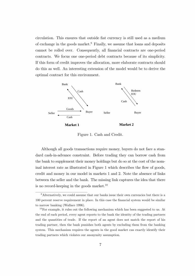
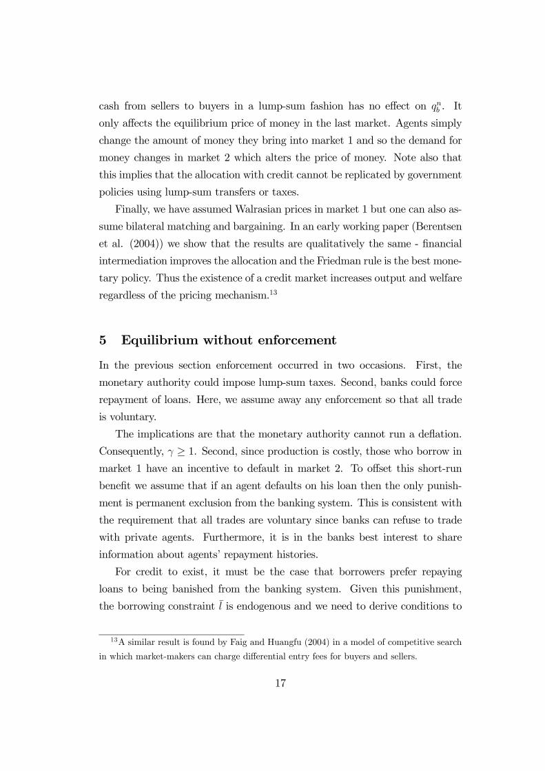
Figure 1. Cash and Credit.

Although all goods transactions require money, buyers do not face a stan-

dard cash-in-advance constraint. Before trading they can borrow cash from

the bank to supplement their money holdings but do so at the cost of the nom-

inal interest rate as illustrated in Figure 1 which describes the flow of goods,

credit and money in our model in markets 1 and 2. Note the absence of links

between the seller and the bank. The missing link captures the idea that there

is no record-keeping in the goods market.10

9Alternatively, we could assume that our banks issue their own currencies but there is a

100 percent reserve requirement in place. In this case the financial system would be similar

to narrow banking (Wallace 1996).10For example, it rules out the following mechanism which has been suggested to us. At

the end of each period, every agent reports to the bank the identity of the trading partners

and the quantities of trade. If the report of an agent does not match the report of his

trading partner, then the bank punishes both agents by excluding them from the banking

system. This mechanism requires the agents in the good market can exactly identify their

trading partners which violates our anonymity assumption.

7

Default. In any model of credit default is a serious issue. We first assume

that banks can force repayment at no cost. In such an environment, default

is not possible so agents face no borrowing constraints. Thgraphics/Figure

1.wmf on how the provision of liquidity via borrowing and lending affects the

allocation. In this case, banks are nothing more than cash machines that

post interest rates for deposits and loans. In equilibrium these posted interest

rates clear the market. We then consider an environment where banks cannot

enforce repayment. The only punishment available is that a borrower who fails

to repay his loan is excluded from the banking sector in all future periods.

Given this punishment, we derive conditions to ensure voluntary repayment

and show that this may involve imposing binding borrowing constraints, i.e.

credit rationing.

3 Symmetric equilibrium

The timing in our model is as follows. At the beginning of the first market

agents observe their production and consumption shocks and they receive the

lump-sum transfers τ 1. Then, the banking sector opens and agents can borrow

and deposit money. Finally, the banking sector closes and agents trade goods.

In the second market agents trade goods and settle financial claims.

In period t, let φ be the real price of money in the second market. We

study equilibria where end-of-period real money balances are time-invariant

φM = φ−1M−1 = Ω (1)

which implies that φ−1φ= γ. We refer to it as a stationary equilibrium.

Consider a stationary equilibrium. Let V (m1) denote the expected value

from trading in market 1 withm1 money balances conditional on the aggregate

shock. Let W (m2, l, d) denote the expected value from entering the second

market with m2 units of money, l loans, and d deposits. In what follows, we

look at a representative period t and work backwards from the second to the

first market.

8

3.1 The second market

In the second market agents produce h goods and consume x, repay loans,

redeem deposits and adjust their money balances. If an agent has borrowed l

units of money, then he pays (1 + i) l units of money, where i is the nominal

loan rate. If he has deposited d units of money, he receives (1 + id) d, where

id is the nominal deposit rate. The representative agent’s program is

W (m2, l, d) = maxx,h,m1,+1

[U (x)− h+ βV (m1,+1)] (2)

s.t. x+ φm1,+1 = h+ φ (m2 + τ 2M−1) + φ (1 + id) d− φ (1 + i) l

where m1,+1 is the money taken into period t + 1 and φ is the real price of

money. Rewriting the budget constraint in terms of h and substituting into

(2) yields

W (m2, l, d) = φ [m2 + τ 2M−1 − (1 + i) l + (1 + id) d]

+ maxx,m1,+1

[U (x)− x− φm1,+1 + βV (m1,+1)] .

The first-order conditions are U 0 (x) = 1 and

φ = βV 0 (m1,+1) (3)

where V 0 (m1,+1) is the marginal value of an additional unit of money taken

into period t+ 1.

Notice that the optimal choice of x is the same across time for all agents

and the m1,+1 is independent of m2. The implication is that regardless of how

much money the agent brings into the second market, all agents enter the

following period with the same amount of money. Those who bring too much

money into the second market, spend the excess cash on goods, while those

with too little money produce extra output to sell for money. As a result, the

distribution of money holdings is degenerate at the beginning of the following

period.

The envelope conditions are

Wm=φ (4)

Wl=−φ (1 + i) (5)

Wd=φ (1 + id) . (6)

9

Note that W (m2, l, d) is linear in its arguments.

Finally, to ensure that all loans can be feasibly repaid in market two, let

v be the ratio of aggregate nominal loan repayments, (1− n) (1 + i) l, to the

money stock,M . If v ≤ 1, then borrowers can repay their loans with one trip tothe bank only since the nominal demand for cash by borrowers for repayment

of loans is less than M . If v > 1, borrowers cannot acquire sufficient balances

in the aggregate to repay loans at once. This implies that they repay part of

their loans which is then used to settle deposit claims and the cash reenters the

goods market as depositors use the cash to acquire more goods. This recycling

of cash occurs until all claims are settled.

3.2 The first market

Let qb and qs respectively denote the quantities consumed by a buyer and

produced by a seller trading in market 1. Let p be the nominal price of goods

in market 1. It is straightforward to show that agents who are buyers will

never deposit funds in the bank and sellers will never take out loans. Thus,

ls = db = 0. In what follows we let l denote loans taken out by buyers and d

deposits of sellers. We also drop these arguments inW (m, l, d) where relevant

for notational simplicity.

An agent who hasm1 money at the opening of the first market has expected

lifetime utility

V (m1) = (1− n) [u (qb) +W (m1 + τ bM−1 + l − pqb, l)]

+n [−c (qs) +W (m1 + τ sM−1 − d+ pqs, d)](7)

where pqb is the amount of money spent as a buyer, and pqs the money received

as a seller. Once the preference shock occurs, agents become either a buyer or

a seller.

Sellers’ decisions. If an agent is a seller in the first market, his problem is

maxqs,d

[−c (qs) +W (m1 + τ sM−1 − d+ pqs, d)]

s.t. d ≤ m1 + τ sM−1

10

The first-order conditions are

−c0 (qs) + pWm=0

−Wm +Wd − λd=0.

where λd is the Lagrangian multiplier on the deposit constraint. Using (4),

the first condition reduces to

c0 (qs) = pφ. (8)

Sellers produce such that the ratio of marginal costs across markets (c0 (qs) /1)

is equal to the relative price (pφ) of goods across markets. Note that qs is

independent of m1 and d. Consequently, sellers produce the same amount

no matter how much money they hold or what financial decisions they make.

Finally, it is straightforward to show that for any id > 0 the deposit constraint

is binding and so sellers deposit all their money balances.

Buyers’ decisions. If an agent is a buyer in the first market, his problem

is:

maxqb,l

[u (qb) +W (m1 + τ bM−1 + l − pqb, l)]

s.t. pqb ≤ m1 + τ bM−1 + l

l ≤ l

Notice that buyers cannot spend more cash than what they bring into the first

market, m1, plus their borrowing, l, and the transfer τ bM−1. He also faces the

constraint that the loan size is constrained by l. For now we assume that this

constraint is arbitrary. However, it is intended to capture the fact that there

is a threshold l above which an agent would choose to default.

Using (4), (5) and (8) the buyers first-order conditions reduce to

u0 (qb)= c0 (qs) (1 + λ/φ) (9)

φi=λ− λl (10)

where λ is the multiplier on the buyer’s cash constraint and λl on the borrowing

constraint. If λ = 0, then (9) reduces to u0 (qb) = c0 (qs) implying trades are

11

efficient.11

For λ > 0, these first-order conditions yield

u0 (qb)

c0 (qs)= 1 + i+ λl/φ

If λl = 0, thenu0 (qb)

c0 (qs)= 1 + i (11)

In this case the buyer borrows up to the point where the marginal benefit of

borrowing equals the marginal cost. He spends all his money and consumes

qb = (m1 + τ bM−1 + l) /p. Note that for i > 0 trades are inefficient. In effect,

a positive nominal interest rate acts as tax on consumption.

Finally, if λl > 0u0 (qb)

c0 (qs)> 1 + i (12)

In this case the marginal value of an extra unit of a loan exceeds the mar-

ginal cost. Hence, a borrower would be willing to pay more than the pre-

vailing loan rate. However, if banks are worried about default, then the

interest rate may not rise to clear the market and credit rationing occurs.

Consequently, the buyer borrows l, spends all of his money and consumes

qb =¡m1 + τ bM−1 + l

¢/p.

Since all buyers enter the period with the same amount of money and face

the same problem qb is the same for all of them. The same is true for the

sellers. Market clearing implies

qs =1− n

nqb. (13)

so that efficiency is achieved at the quantity q∗ solving u0 (q∗) = c0¡1−nnq∗¢.

Banks. Banks accept nominal deposits, paying the nominal interest rate id,

and make nominal loans l at nominal rate i. The banking sector is perfectly

competitive, so banks take these rates as given. There is no strategic inter-

action among banks or between banks and agents. In particular, there is no

11With 1 − n buyers and n sellers, the planner maximizes (1− n)u (qb) − nc (qs) s.t.

(1− n) qb = nqs. Use the constraint to replace qs in the maximand. The first-order condition

for qb is u0 (qb) = c0 (qs).

12

bargaining over terms of the loan contract. Finally, we assume that there are

no operating costs or reserve requirements.

The representative bank solves the following problem per borrower

maxl(i− id) l

s.t. l ≤ l

u (qb)− (1 + i) lφ ≥ Γ

where Γ is the reservation value of the borrower. The reservation value is the

borrower’s surplus from receiving a loan at another bank. We investigate two

assumptions about the borrowing constraint l. In the first case, banks can

force repayment at no cost. In this case the borrowing constraint is exogenous

and we set it to l =∞. In the second case, we assume that a borrower who failsto repay his loan will be shut out of the banking sector in all future periods.

Given this punishment, the borrowing constraint is endogenous and we need

to derive conditions to ensure voluntary repayment.

The first-order condition is

i− id − λL + λΓ

∙u0 (qb)

dqbdl− (1 + i)φ

¸= 0

where λL ≥ 0 is the Lagrange multiplier on the lending constraint and λΓ

on the participation constraint of the borrower. Profit maximization implies

λΓ > 0.

In any competitive equilibrium the banks make no profit so i = id. Since,dqbdl= φ/c0 (qs) we have

u0 (qb)

c0 (qs)= 1 + i+

λLλΓφ

.

If repayment is not an issue, λL = 0 and so the loan offered by the bank

satisfies (11). If the constraint on the loan size is binding, i.e. λL > 0, it

satisfies (12).

In a symmetric equilibrium all buyers borrow the same amount, l, and

sellers deposit the same amount, d, where profit maximization implies

(1− n) l = nd. (14)

13

Marginal value of money. Using (7) the marginal value of money is

V 0 (m1) = (1− n)u0 (qb)

p+ nφ (1 + id) .

In the appendix we show that the value function is concave inm so the solution

to (3) is well defined.

Using (8) V 0 (m1) reduces to

V 0 (m1) = φ

∙(1− n)

u0 (qb)

c0 (qs)+ n (1 + id)

¸. (15)

Note that banks increase the marginal value of money because sellers can

deposit idle cash and earn interest. This is is captured by the second term on

the right-hand side. If there are no banks, this term is just n.

4 Equilibrium with enforcement

In this section as a benchmark we assume that the monetary authority can

impose lump-sum taxes and that banks can force repayment of loans at no

cost. Note that this does not imply that the banks or the monetary authority

can dictate the terms of trade between private agents in the goods market.

In any stationary monetary equilibrium use (3) lagged one period to elim-

inate V 0 (m1) from (15). Then use (1) and (13) to get

γ − β

β= (1− n)

"u0 (qb)

c0¡1−nnqb¢ − 1#+ nid. (16)

The right-hand side measures the value of bringing one extra unit of money

into the first market. The first term reflects net benefit (marginal utility minus

marginal cost) of spending the unit of money on goods when a buyer and the

second term is the value of depositing an extra unit of idle balances when a

seller.

Since banks can force agents to repay their loans, agents are unconstrained

14

and so l =∞. This implies that (11) holds. Using it in (16) yields12

γ − β

β= (1− n) i+ nid. (17)

Now, the first term on the right-hand side reflects the interest saving from

borrowing one less unit of money when a buyer.

Zero profit implies i = id and so

γ − β

β= i. (18)

We can rewrite this in terms of qb using (11) to get

γ − β

β=

u0 (qb)

c0¡1−nnqb¢ − 1. (19)

Definition 1 When repayment of loans can be enforced, a monetary equilib-

rium with credit is an interest rate i satisfying (18) and a quantity qb satisfying

(19).

Proposition 1 Assume repayment of loans can be enforced. Then if γ ≥ β, a

monetary equilibrium with credit exists and is unique for γ > β. Equilibrium

consumption is decreasing in γ, and satisfies qb < q∗ with qb → q∗ as γ → β.

It is clear from (19) that money is neutral, but not super-neutral. In-

creasing its stock has no effect on qb, while changing the growth rate γ does.

Moreover, the Friedman rule generates the first-best allocation.

How does this allocation differ from the allocation in an economy with-

out credit? Let qnb denote the quantity consumed in such an economy. It is

straightforward to show that qnb solves (16) with id = 0, i.e.,

γ − β

β= (1− n)

"u0 (qnb )

c0¡1−nnqnb¢ − 1# . (20)

Comparing (20) to (19), it is clear that qnb < qb for any γ > β.

12This equation implies that if nominal bonds could be traded in market 2, then their

nominal rate of return ib would be (1− n) i + nid. For µ = 0 the return would be i = id.

Thus agents would be indifferent between holding a nominal bond or holding a bank deposit.

15

Corollary 1 When γ > β, financial intermediation improves the allocation

and welfare.

The key result of this section is that financial intermediation improves the

allocation away from the Friedman rule. The greatest impact on welfare is for

moderate values of inflation. The reason is that near the Friedman rule there is

little gain from redistributing idle cash balances while for high inflation rates

money is of little value anyway. At the Friedman rule agents can perfectly

self-insure against consumption risk because the cost of holding money is zero.

Consequently, there is no welfare gain from financial intermediation.

Given that banks improve the allocation away from the Friedman rule, is

it because they relax borrowers’ liquidity constraints or because they allow

payment of interest to depositors? The following Proposition answers this

question.

Proposition 2 The gain in welfare from financial intermediation is due to

the fact that it allows payment of interest to depositors and not from relaxing

borrowers’ liquidity constraints

According to Proposition 2 the gain in welfare comes from payment of in-

terest to agents holding idle balances. To prove this claim we show in the proof

of Proposition 2 that in equilibrium, agents are indifferent between borrowing

to finance equilibrium consumption or holding the amount of cash that allows

them to acquire the same amount without borrowing. The only importance

of borrowing is to sustain payment of interest to depositors. That is, even

though each individual agent is indifferent between borrowing and not bor-

rowing, agents taking out loans are needed to finance the interest received by

the depositors.

As a final proof of this argument, we consider a systematic government pol-

icy that redistributes cash in market 1 by imposing lump-sum taxes on sellers

and giving the cash as lump-sum transfers to buyers. This clearly relaxes

the liquidity constraints of the buyers while paying no interest to depositors.

However, inspection of (20) reveals that neither τ 1 nor τ b appear in this equa-

tion. Hence, varying the transfer across the two markets or by redistributing

16

cash from sellers to buyers in a lump-sum fashion has no effect on qnb . It

only affects the equilibrium price of money in the last market. Agents simply

change the amount of money they bring into market 1 and so the demand for

money changes in market 2 which alters the price of money. Note also that

this implies that the allocation with credit cannot be replicated by government

policies using lump-sum transfers or taxes.

Finally, we have assumed Walrasian prices in market 1 but one can also as-

sume bilateral matching and bargaining. In an early working paper (Berentsen

et al. (2004)) we show that the results are qualitatively the same - financial

intermediation improves the allocation and the Friedman rule is the best mone-

tary policy. Thus the existence of a credit market increases output and welfare

regardless of the pricing mechanism.13

5 Equilibrium without enforcement

In the previous section enforcement occurred in two occasions. First, the

monetary authority could impose lump-sum taxes. Second, banks could force

repayment of loans. Here, we assume away any enforcement so that all trade

is voluntary.

The implications are that the monetary authority cannot run a deflation.

Consequently, γ ≥ 1. Second, since production is costly, those who borrow inmarket 1 have an incentive to default in market 2. To offset this short-run

benefit we assume that if an agent defaults on his loan then the only punish-

ment is permanent exclusion from the banking system. This is consistent with

the requirement that all trades are voluntary since banks can refuse to trade

with private agents. Furthermore, it is in the banks best interest to share

information about agents’ repayment histories.

For credit to exist, it must be the case that borrowers prefer repaying

loans to being banished from the banking system. Given this punishment,

the borrowing constraint l is endogenous and we need to derive conditions to

13A similar result is found by Faig and Huangfu (2004) in a model of competitive search

in which market-makers can charge differential entry fees for buyers and sellers.

17

ensure voluntary repayment. In what follows, since the transfers only affect

prices, we set τ b = τ s = τ 1.

For buyers entering the second market with no money and who repay their

loans, the expected discounted utility in a steady state is

U = U (x∗)− hb + βV (m1,+1 )

where hb is a buyer’s production in the second market if he repays his loan.

Consider the case of a buyer who reneges on his loan. The benefit of

reneging is that he has more leisure in the second market because he does not

work to repay the loan. The cost is that he is out of the banking system,

meaning that he cannot borrow or deposit funds for the rest of his life. He

cannot lend because the bank would confiscate his deposits to settle his loan

arrears. Thus, a deviating buyer’s expected discounted utility is

bU = U (bx)− bhb + βbV (m1,+1 )

where the hat indicates the optimal choice by a deviator. The value of being

in the banking system U as well as the expected discounted utility of defectionbU depend on the growth rate of the money supply γ. This puts constraints

on γ that the monetary authority can impose without destroying financial

intermediation.

Existence of a monetary equilibriumwith credit requires that U ≥ bU , wherethe borrowing constraint l satisfies

U = bU . (21)

In the proof of Proposition 3 we show that l satisfies

l =β

φ (1 + i) (1− β)

½(1− n)Ψ+ c0 (qs)

µγ − β

β

¶[bqb − (1− n) qb]

¾(22)

whereΨ = u (qb)−u (bqb)−c0 (qs) (qb − bqb) ≥ 0. In an unconstrained equilibriumwith credit we have l ≤ l and in a constrained equilibrium l = l.

In order to determine the sign of l, we need to determine whether a devi-

ator carries more money than a non-deviator since in (22) bqb − (1− n) qb =

18

(m1 −m1) /p. This in turn depends on his degree of risk aversion. It is reason-

able to assume that the deviator is sufficiently risk averse that he holds more

real balances to compensate for the loss of consumption insurance provided

by the banking system. In the appendix we show that a sufficient condition

for this to be true is that the degree of relative risk aversion is greater than

one. If this condition holds, then bqb − (1− n) qb > 0 for any γ ≥ 1 so l is

non-negative.

In any equilibrium, profit maximization implies that banks lend out all of

their deposits. This implies that (14) holds also in a constrained equilibrium,

i.e.,

l =n

1− nM.

To guarantee repayment in a constrained equilibrium banks charge a nominal

loan rate, ı, that is below the market clearing rate.14

Definition 2 A monetary equilibrium with unconstrained credit is a triple

(qb, bqb, i) satisfyingγ − β

β=(1− n)

∙u0 (qb)

c0 (qs)− 1¸+ ni (23)

γ − β

β=(1− n)

∙u0 (bqb)c0 (qs)

− 1¸

(24)

u0 (qb)

c0 (qs)=1 + i (25)

such that 0 < φl = nc0 (qs) qb < φl, where qs = 1−nnqb.

Definition 3 Amonetary equilibrium with constrained credit is a triple (qb, bqb, ı)satisfying (23), (24) and (22) where nc0 (qs) qb = φl and qs = 1−n

nqb.

14This may seem counter-intuitive since one would think that banks would reduce l to

induce repayment. However, this cannot be an equilibrium since it would imply that banks

are not lending out all of their deposits. If banks are not lending out all of their deposits

then zero profits would require id = (1− µ) i where µ is the fraction of deposits held idle by

the bank. If all banks were to choose a triple (i, id, µ) with µ > 0 such that they earned zero

profits, then a bank could capture the entire market and become a monopolist by raising idby an infinitesimal amount and lowering µ and i by an infinitesimal amount. Since all banks

can do this, in a constrained equilibrium, the only feasible solution is µ = 0 and i = id = ı.

19

Proposition 3 Let the degree of risk aversion be greater than one. Then

there exists a critical value β such that if β ≥ β there is a eγ > 1 such that the

following is true:

(i) If γ > eγ, a unique monetary equilibrium with unconstrained credit exists.

(ii) If 1 < γ ≤ eγ, a monetary equilibrium with constrained credit may exist.

(iii) If γ = 1, no monetary equilibrium with credit exists.

According to Proposition 3, existence of a monetary equilibrium with credit

requires that there is some inflation. The reason for this is quite intuitive. If a

borrower works to repay his loan in market 2, he is strictly worse off than when

he defaults since the outside option (trading with money only) yields almost

the efficient consumption q∗ in all future periods. With zero inflation, agents

are able to self-insure at low cost, thus having access to financial markets is of

little value. As a result, borrowers will not repay their loans and so financial

intermediation is impossible. This result is related to Aiyagari and Williamson

(2000) who also report a break-down of financial intermediation in a dynamic

contracting model with private information close to the Friedman rule.

For small rates of inflation credit rationing occurs. Again, for low rates of

inflation the cost of using money to self-insure is low. To induce repayment

banks charge a below market-clearing interest rate since this reduces the total

repayment the borrowers have to make. In short, with an endogenous bor-

rowing constraint, the interest rate is lower than would occur in an economy

where banks can force repayment.15

One aspect that is puzzling about this result is that the incentive to de-

fault is higher for low nominal interest rates and lower for high nominal in-

terest rates. This seems counter-intuitive at first glance since standard credit-

rationing models, such as Stiglitz and Weiss (1981), suggest that the likelihood

of default increases as interest rates rise. The reason for the difference in results

is that standard credit rationing models focus on real interest rates, while our

model is concerned with nominal interest rates. In our model, nominal rates

rise because of perfectly anticipated inflation, which acts as a tax on deviators’

15This result is similar to results reported in Kehoe and Levine (1993), Alvarez and

Jermann (2000) or Hellwig and Lorenzoni (2004).

20

wealth since they carry more money for transactions purposes. This reduces

the incentive to default thereby alleviating the need to ration credit. Conse-

quently, a key contribution of our analysis is to show how credit rationing can

arise from changes in nominal interest rates.

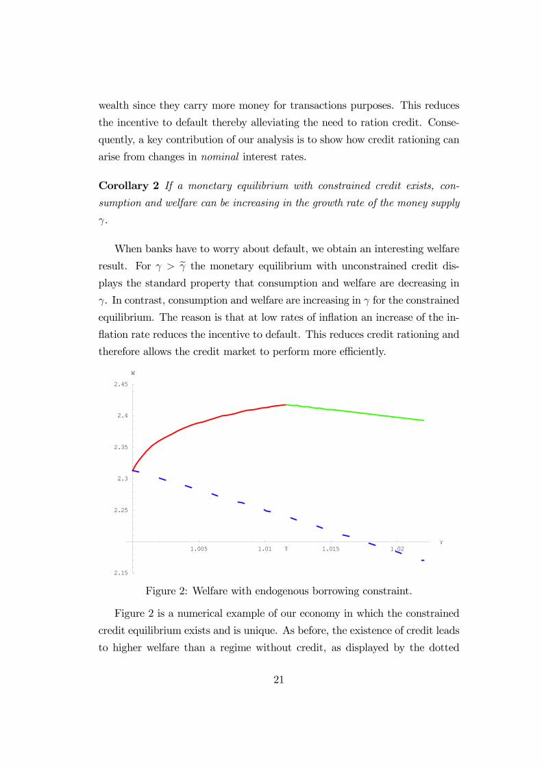
Corollary 2 If a monetary equilibrium with constrained credit exists, con-

sumption and welfare can be increasing in the growth rate of the money supply

γ.

When banks have to worry about default, we obtain an interesting welfare

result. For γ > eγ the monetary equilibrium with unconstrained credit dis-

plays the standard property that consumption and welfare are decreasing in

γ. In contrast, consumption and welfare are increasing in γ for the constrained

equilibrium. The reason is that at low rates of inflation an increase of the in-

flation rate reduces the incentive to default. This reduces credit rationing and

therefore allows the credit market to perform more efficiently.

1.005 1.01 1.015 1.02γ

2.15

2.25

2.3

2.35

2.4

2.45

W

γ

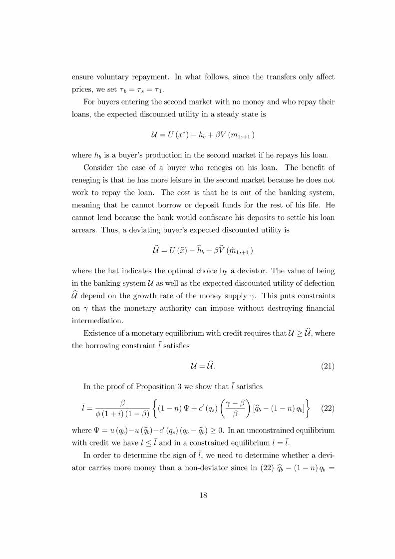
Figure 2: Welfare with endogenous borrowing constraint.

Figure 2 is a numerical example of our economy in which the constrained

credit equilibrium exists and is unique. As before, the existence of credit leads

to higher welfare than a regime without credit, as displayed by the dotted

21

blue line, even when credit is rationed. It also illustrates that with credit

welfare rises with inflation for the constrained equilibrium while it falls in the

unconstrained equilibrium.

6 Conclusion

In this paper we have shown how money and credit can coexist in an essential

model of money. Our main findings is that financial intermediation in general

improves the allocation. If enforcement exists, the optimal monetary policy is

the Friedman rule and it generates the first-best allocation. If not, then the

optimal policy may require a positive rate of inflation.

Our framework is open to many extensions such as private bank note issue,

financing of investment instead of consumption, and other financial contracts.

We could also extend the model to investigate the role of banks in transmitting

other type of shocks such as productivity shocks or preference shocks. Finally,

the interaction of government regulation and stabilization policies would allow

analysis of different monetary arrangementIKT24P00.wmfpressed by the real-

bill doctrine or the quantity theory as studied in Sargent and Wallace (1982).

22

References

Aiyagari, S. and S. Williamson (2000). “Money and Dynamic Credit Arrange-

ments with Private Information.” Journal of Economic Theory 91, 248-279.

Alvarez, F. and U. Jermann (2000). “Efficiency, Equilibrium and Asset Pricing

with Risk of Default.” Econometrica, 68 (4), 775-797.

Aruoba, B., C. Waller and R. Wright (2003). “Money and Capital.” Working

paper, University of Pennsylvania.

Berentsen, A., G. Camera and C. Waller (2004a). “The Distribution of Money

and Prices in an Equilibrium with Lotteries.” Economic Theory, Volume 24,

Number 4, p. 887 - 906 .

Berentsen, A., G. Camera and C. Waller, “Money, Credit and Banking", IEW

Working Paper No. 219 (2004).

Berentsen, A., G. Camera and C. Waller (2005). “The Distribution of Money

Balances and the Non-Neutrality of Money.” International Economic Review,

46, 465-487.

Bewley, T. (1980). “The Optimum Quantity of Money,” in John H. Karaken

and Neil Wallace, eds., Models of Monetary Economics, Minneapolis: Federal

Reserve Bank of Minneapolis, 1980, 169-210.

Camera, G. and D. Corbae (1999). “Money and Price Dispersion.” Interna-

tional Economic Review 40, 985-1008.

Cavalcanti, R. and N. Wallace (1999a). “Inside and Outside Money as Alter-

native Media of Exchange.” Journal of Money, Credit, and Banking, 31 (3)

Part 2, 443-457.

Cavalcanti, R., and N.Wallace (1999b). “AModel of Private Bank-note Issue.”

Review of Economic Dynamics, 2 (1), 104-136.

Cavalcanti, R., Erosa, A. and T. Temzelides (1999). “Private Money and Re-

serve Management in a Random-Matching Model.” Journal of Political Econ-

omy, 107 (5), 929-945.

Faig, M. (2004). “Money and Banking in an Economy with Villages” Working

paper, University of Toronto.

Faig, M. and X. Huangfu (2004). “Competitive Search Equilibrium in Mone-

tary Economies.” Working paper, University of Toronto.

23

Green, E. and R. Zhou, (2005). “Money as a Mechanism in a Bewley Econ-

omy.” International Economic Review, 46, 351-371.

He, P., L. Huang and R. Wright (2005). “Money and Banking in Search

Equilibrium.” International Economic Review, 46, 637-670.

Hellwig, C. and G. Lorenzoni (2004). “Bubbles and Private Liquidity.” Work-

ing paper, UCLA.

Kehoe, T. and D. Levine (1993). “Debt-Constrained Asset Markets.” Review

of Economic Studies, 60, 865-888.

Kocherlakota, N. (1998). “Money is Memory.” Journal of Economic Theory,

81, 232—251.

Kocherlakota, N. (2003). “Societal Benefits of Illiquid Bonds.” Journal of

Economic Theory, 108, 179-193.

Lagos, R. and R. Wright (2005). “A Unified Framework for Monetary Theory

and Policy Evaluation.” Journal of Political Economy 113, 463-484.

Lagos, R. and G. Rocheteau (2005). “Inflation, Output and Welfare.” Inter-

national Economic Review, 46, 495-522.

Levine, D. (1991). “Asset Trading Mechanisms and Expansionary Policy.”

Journal of Economic Theory, 54, 148-164.

Lucas, R. E. (1980). “Equilibrium in a Pure Currency Economy,” in John H.

Karaken and Neil Wallace, eds., Models of Monetary Economics, Minneapolis:

Federal Reserve Bank of Minneapolis, 1980.

Rocheteau, G. and R. Wright (2005). “Money in Search Equilibrium, in Com-

petitive Equilibrium and in Competitive Search Equilibrium.” Econometrica,

73, 175-202.

Sargent, T. and N. Wallace (1982). “The Real-Bills Doctrine versus the Quan-

tity Theory: A Reconsideration.” Journal of Political Economy, 90 (6), 1212-

1236.

Shi, S. (1996). “Credit and Money in a Search Model with Divisible Com-

modities.” Review of Economic Studies, 63, 627-652.

Stiglitz, J. and A. Weiss (1981). “Credit Rationing in Markets with Imperfect

Information.” American Economic Review, 71, 393-410.

Wallace, N. (1996). “Narrow Banking Meets the Diamond-Dybvig Model.”

24

Quarterly Review, Vol. 20, No. 1, Winter 1996, 3—13.

Wallace, N. (2001). “Whither Monetary Economics?” International Economic

Review, 42, 847-869.

25

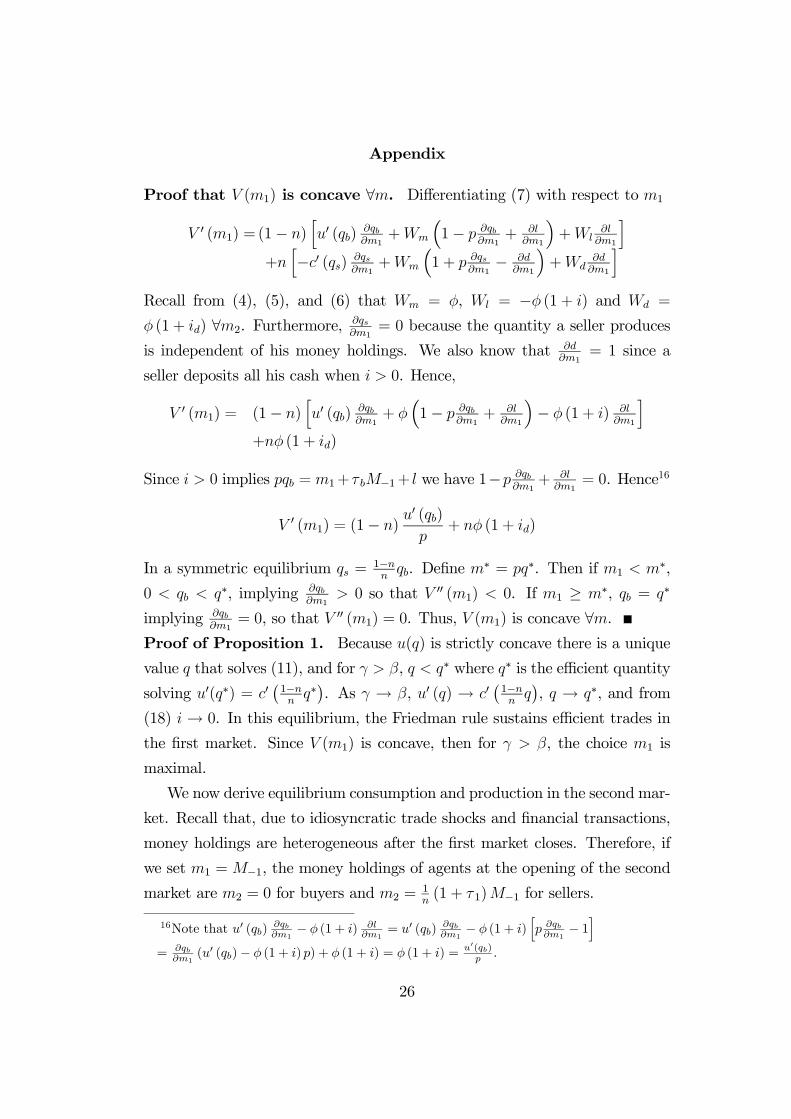
Appendix

Proof that V (m1) is concave ∀m. Differentiating (7) with respect to m1

V 0 (m1) = (1− n)hu0 (qb)

∂qb∂m1

+Wm

³1− p ∂qb

∂m1+ ∂l

∂m1

´+Wl

∂l∂m1

i+nh−c0 (qs) ∂qs

∂m1+Wm

³1 + p ∂qs

∂m1− ∂d

∂m1

´+Wd

∂d∂m1

iRecall from (4), (5), and (6) that Wm = φ, Wl = −φ (1 + i) and Wd =

φ (1 + id) ∀m2. Furthermore,∂qs∂m1

= 0 because the quantity a seller produces

is independent of his money holdings. We also know that ∂d∂m1

= 1 since a

seller deposits all his cash when i > 0. Hence,

V 0 (m1) = (1− n)hu0 (qb)

∂qb∂m1

+ φ³1− p ∂qb

∂m1+ ∂l

∂m1

´− φ (1 + i) ∂l

∂m1

i+nφ (1 + id)

Since i > 0 implies pqb = m1+τ bM−1+ l we have 1−p ∂qb∂m1

+ ∂l∂m1

= 0. Hence16

V 0 (m1) = (1− n)u0 (qb)

p+ nφ (1 + id)

In a symmetric equilibrium qs =1−nnqb. Define m∗ = pq∗. Then if m1 < m∗,

0 < qb < q∗, implying ∂qb∂m1

> 0 so that V 00 (m1) < 0. If m1 ≥ m∗, qb = q∗

implying ∂qb∂m1

= 0, so that V 00 (m1) = 0. Thus, V (m1) is concave ∀m.Proof of Proposition 1. Because u(q) is strictly concave there is a unique

value q that solves (11), and for γ > β, q < q∗ where q∗ is the efficient quantity

solving u0(q∗) = c0¡1−nnq∗¢. As γ → β, u0 (q) → c0

¡1−nnq¢, q → q∗, and from

(18) i → 0. In this equilibrium, the Friedman rule sustains efficient trades in

the first market. Since V (m1) is concave, then for γ > β, the choice m1 is

maximal.

We now derive equilibrium consumption and production in the second mar-

ket. Recall that, due to idiosyncratic trade shocks and financial transactions,

money holdings are heterogeneous after the first market closes. Therefore, if

we set m1 =M−1, the money holdings of agents at the opening of the second

market are m2 = 0 for buyers and m2 =1n(1 + τ 1)M−1 for sellers.

16Note that u0 (qb)∂qb∂m1− φ (1 + i) ∂l

∂m1= u0 (qb)

∂qb∂m1− φ (1 + i)

hp ∂qb∂m1− 1i

= ∂qb∂m1

(u0 (qb)− φ (1 + i) p) + φ (1 + i) = φ (1 + i) = u0(qb)p .

26

Equation (3) gives us x∗ = U 0−1 (1). The buyer’s production in the second

market can be derived as follows

hb = x∗ + φ m1,+1 + (1 + i) l − τ 2M−1 = x∗ + c0 (qs) qb + φil

since in equilibrium

m1,+1 =M =M−1 + τ 1M−1 + τ 2M−1 and c0 (qs) qb = φ [(1 + τ 1)M−1 + l] .

Thus, an agent who was a buyer in market 1 has to work to recover the

production cost of his consumption and the interest on his loan. The seller’s

production is

hs=x∗ + φ m1,+1 − [pqs + (1 + τ 1)M−1 + idd+ τ 2M−1]

=x∗ − c0 (qs) qs − φidd

The expected hours worked h satisfies

h = (1− n)hb + nhs = x∗ (26)

since in equilibrium qb =n1−nqs and i (1− n) l = idnd. Finally, hours in market

2 can be also expressed in terms of q as in the following tableTrading history: Production in the last market:

Buy hb = x∗ + c0 (qs) (1− n) qb + ne (qb)u (qb)

Sell hs = x∗ − (1−n)n[c0 (qs) (1− n) qb + ne (qb)u (qb)]

Since we assumed that the elasticity of utility e (qb) is bounded, we can

scale U(x) such that there is a value x∗ = U 0−1 (1) greater than the last term

for all qb ∈ [0, q∗]. Hence, hs is positive for for all qb ∈ [0, q∗] ensuring that theequilibrium exists.

Proof of Proposition 2. Assume that at some point in time t an agent

at the beginning of market 2 chooses never to borrow again but continues to

deposit. The first thing to note is that it is optimal for him to buy the same

quantity qb since his optimal choice still satisfies (19). This implies that his

money balances are m1,+1 = m1,+1 + l+1. An agent who decides to opt out

from borrowing has to carry more money but he saves the interest on loans

in the future. In particular, consumption and production in the market 1 are

27

not affected. The difference in lifetime payoffs come from difference in hours

worked.

If he enters market 2 having been a buyer, the hours worked are

hb=x∗ + φ m1,+1 + l+1 + (1 + i) l − τ 2M−1

=x∗ + c0 (qs) qb + φl+1 + φil

while if he sold in market 1 he works

hs=x∗ + φ m1,+1 + l+1 − [pqs + (1 + i) d+ τ 2M−1]

=x∗ − c0 (qs) qs + φl+1 − φidd

The expected hours worked satisfy

h = (1− n) hb + nhs = x∗ + φl+1

Consequently, from (26) the additional hours worked are

h− h = φl+1 = γnc0 (qs) qb > 0 (27)

since l+1 = γl in a steady state.

Let us next consider the hours worked in market 2 in some future period.

Since he has no loan to repay the hours worked are

hb=x∗ + φ m1,+1 + l+1 − τ 2M−1

=x∗ + φ M−1 + τ 1M−1 + l + l+1 − l

=x∗ + c0 (qs) qb + φl (γ − 1)

=x∗ + c0 (qs) qb + nc0 (qs) qb (γ − 1)

if he was a buyer while if he sold in market 1 he works

hs=x∗ + φ©m1,+1 + l+1 −

£pqs + (1 + i) d+ τ 2M−1

¤ª=x∗ + φ

©M−1 + τ 1M−1 + l + l+1 − l −

£pqs + (1 + i) d

¤ª=x∗ + c0 (qs) qb + φl (γ − 1)− φ

£pqs + (1 + i) d

¤=x∗ + c0 (qs) qb + φl (γ − 1)− c0 (qs) qs − φ (1 + i) pqb

=x∗ + nc0 (qs) qb (γ − 1)− c0 (qs) qs − ic0 (qs) qb

=x∗ + nc0 (qs) qb (γ − 1)− c0 (qs) qs − (γ − β) c0 (qs) qb/β

28

The expected hours worked h satisfies

h = (1− n) hb + nhs = x∗ − nc0 (qs) qbγ (1− β) /β

The expected gain from this strategy in any future period is

h− h = −nc0 (qs) qbγ (1− β) /β < 0 (28)

Then, from (27) and (28), the total expected gain from this deviation is

h− h+β³h− h

´1− β

= 0.

So agents are indifferent to borrow at the current rate of interest or taking in

the equivalent amount of money themselves.

Proof of Corollary ??. Neither τ 1 nor τ b appear in (19). Therefore, (τ 1, τ 2)

can only affect the equilibrium φ. Of course, by changing τ 1 we change τ 2, for

a given rate of growth of money. To see how the transfers affect φ note that

φl = c0(qs)nqb. Since l = n1−nM−1(1 + τ s) =

n1−nM(

1+τs1+τ

) and qs =1−nnqb then

we have

φ =c0(qs)nqb

l=(1− n)c0(1−n

nqb) (1 + τ)

M(1 + τ s)

which implies the price of money in the second market, φ, is affected by the

timing and size of lump-sum transfers.

Proof of Proposition 3. Since the transfers do not affect quantities set

τ b = τ s = τ 1. We now derive the endogenous borrowing constraint l. This

quantity is the maximal loan that a borrower is willing to repay in the second

market at given market prices. For buyers entering the second market with

no money, who repay their loans, the expected discounted utility in a steady

state is

U = U (x∗)− hb + βV (m1,+1 )

where hb is a buyer’s production in the second market if he repays his loan.

A deviating buyer’s expected discounted utility is

bU = U (bx)− bhb + βbV (m1,+1 )

where the hat indicates the optimal choice by a deviator.

29

We now derive bx, bhb, bqb, and bqs. In the last market the deviating buyer’sprogram is

cW (m2)= maxx,h,m1,+1

hU (bx)− bhb + β bV (m1,+1)

is.t. bx+ φm1,+1 = bhb + φ (m2 + τ 2M−1)

As before, the first-order conditions are U 0 (bx) = 1 and−φ+ βbV 0 (m1,+1) = 0. (29)

Thus, bx = x∗. The first-order condition if the deviator is a seller in the first

market is −c0 (bqs) + pφ = 0. Hence, the deviator produces the same amount

as non-deviating sellers so bqs = qs =1−nnqb.

Finally, the marginal value of the money satisfies

bV 0 (m1) = φ

∙(1− n)u0 (bqb)

c0 (qs)+ n

¸which means that (29) can be written as

γ − β

β= (1− n)

∙u0 (bqb)c0 (qs)

− 1¸. (30)

Now if we compare (30) with (19) we find that

1− n =u0 (qb)− c0 (qs)

u0 (bqb)− c0 (qs)(31)

implying bqb < qb.

The money holdings of the deviator grows at rate γ since from (30) bqb isconstant across time. The money holdings of the deviator at the opening of

the second market are m2 = 0 having bought and m2 = m1 + τ 1M−1 + pqs

having sold. Thus, hours worked are

bhb=x∗ + φ [m1,+1 − τ 2M−1] = x∗ + c0 (qs) bqb + φ (γ − 1) (m1 −M−1) (32)bhs=x∗ + φ [m1,+1 − (m1 + τ 1M−1)− pbqs − τ 2M−1]

=x∗ − c0 (qs) qs + φ (γ − 1) (m1 −M−1) (33)

since for a deviator pbqb = m1+τ 1M−1. The term φ (γ − 1) (m1 −M−1) reflects

the fact that the deviator is subject to the inflation tax in a different way than

the representative agent.

30

Since pqb =11−n (1 + τ 1)M−1 in equilibrium and pbqb = m1 + τ 1M−1 it

follows that φ (γ − 1) (m1 −M−1) = c0 (qs) (γ − 1) [bqb − (1− n) qb]. Hence, the

expected hours worked for a deviator are

bh = x∗ + c0 (qs) (1− n) (bqb − qb) + (γ − 1) [bqb − (1− n) qb] (34)

The endogenous borrowing constraint l satisfies U¡l¢= bU . To derive l

note that for a buyer who took out a loan of size l the hours worked at night

are

hb=x∗ + φ£m1,+1 + (1 + i) l − τ 2M−1

¤=x∗ + c0 (qs) qb + φ (1 + i) l − φl

Hence from U¡l¢= bU we have

U (x∗)− hb + βV (m1,+1 ) = U (bx)− bhb + βbV (m1,+1 )

where bhb satisfies (32). Since bx = x∗ we have

bhb − hb = βhbV (m1,+1 )− V (m1,+1 )

iso

φ (1 + i) l = γc0 (qs) [bqb − (1− n) qb] + βhV (m1,+1 )− bV (m1,+1 )

i(35)

since φl = nc0 (qs) qb.

Finally, the continuation payoffs are

bV (m1,+1 )=∞Xt=0

βth(1− n)u (bqb)− nc (qs) + U (x∗)− bhi

V (m1,+1 )=∞Xt=0

βt [(1− n)u (qb)− nc (qs) + U (x∗)− h] .

In a steady state the difference is

V (m1,+1 )− bV (m1,+1 )=n(1− n) [u (qb)− u (bqb)] + bh− h

o(1− β)−1

= (1− n)Ψ+ c0 (qs) (γ − 1) [bqb − (1− n) qb] (1− β)−1 .

where Ψ = u (qb)− u (bqb)− c0 (qs) (qb − bqb). Sinceu (qb)− u (bqb)

qb − bqb > u0 (qb) > c0 (qs)

31

for all γ > β, it follows that Ψ > 0. Consequently, (35) can be written as

l =β

φ (1 + i) (1− β)

½(1− n)Ψ+ c0 (qs)

µγ − β

β

¶[bqb − (1− n) qb]

¾.

Unconstrained credit equilibrium. In an unconstrained equilibrium

we have unique values of qb and i. All that is left is to show is that l ≤ l, or

φ (1 + i) l = (1 + i)nqb ≤β

1− β

½(1− n)Ψ+ c0 (qs)

µγ − β

β

¶[bqb − (1− n) qb]

¾Since in an unconstrained equilibrium (11) and (20) hold, we need

nqbu0 (qb) (1− β) ≤ β (1− n) Ψ+ [u0 (bqb)− c0 (qs)] [bqb − (1− n) qb] (36)

We need to determine the sign of bqb − (1− n) qb. Using (31) we obtain

bqb − (1− n) qb =bqbu0 (bqb)− qbu

0 (qb)

u0 (bqb)− c0 (qs)+

c0 (qs) (qb − bqb)u0 (bqb)− c0 (qs)

Since qb ≥ bqb for all γ, a sufficient condition for bqb − (1− n) qb ≥ 0 is thatqu0 (q) is monotonically decreasing in q. This is equivalent to having R(q) =

−qu00(q)/u0(q) ≥ 1 for all q ∈ [0, q∗]. If this condition holds, then l ≥ 0 for anyγ ≥ β.

Define

g (γ)≡nqbu0 (qb) (1− β)

f (γ)≡β (1− n) Ψ+ [u0 (bqb)− c0 (qs)] [bqb − (1− n) qb]

Then, g (β) = nq∗ (1− β) > 0 and f (β) = 0. Thus, the repayment constraint

is violated at the Friedman rule.

It can be shown that

f 0 (γ)= c0 (qs) [bqb − (1− n) qb]−c00 (qs) c

0 (qs)2 (1− n)2 nqb

[nu00 (qb) c0 (qs)− u0 (qb) c00 (qs) (1− n)]> 0

g0 (γ)=n (1− β)u0 (qb) [1−R(q)]dqbdγ≥ 0

Since g(β) > f(β), a sufficient condition for uniqueness, should an equilibrium

exist, is g0 (γ) < f 0 (γ) for all γ or

n (1− β) [u0 (qb) + qbu00 (qb)]

dqbdγ

<

β (1− n) u00 (qb) [bqb − (1− n) qb]dbqbdγ− β (1− n)2 c00 (qs) qb

dqbdγ

.

32

We also have, from (31),

dbqbdγ

=u00 (qb)− c00 (qs) (1− n)

(1− n)u00 (bqb) dqbdγ

< 0.

Thus after some algebra we have

n (1− β)u0 (qb)dqbdγ

<

β

∙bqb − (1− n) qb − n

µ1− β

β

¶qb

¸u00 (qb)

dqbdγ− βbqbc00 (qs) (1− n)

dqbdγ

The left hand side is negative. The second term on the RHS is positive. The

first term will be non-negative for β close to one. Thus, for β sufficiently close

to one, if an equilibrium exists it is unique.

To establish existence, note that as β → 1, g (β) → f (β). Since f 0 (γ) >

g0 (γ) for all γ as β → 1, it then follows that for β ∈³β, 1

´an equilibrium

exists for all γ greater than a finite value γ and it is unique.

Constrained credit equilibriumWe now consider 1 ≤ γ < γ. In a con-

strained equilibrium the defection constraint must hold with equality implying

(1 + ı)nc0 (qs) qb =β

1− β

½(1− n)Ψ+ c0 (qs)

µγ − β

β

¶[bqb − (1− n) qb]

¾(37)

where qb denotes the quantity consumed and ı is the interest rate in a con-

strained equilibrium. From the first-order conditions on money holdings we

have

γ − β

β=(1− n)

∙u0 (qb)

c0 (qs)− 1¸+ nı (38)

γ − β

β=(1− n)

∙u0 (bqb)c0 (qs)

− 1¸

(39)

where qs = 1−nnqb. Thus, a constrained equilibrium is a list qb, bqb, ı such that

(37)-(39) hold.

We now investigate the properties of (37)-(39). At ı = 0, from (38) and

(39), qb = bqb. Then from (37) we have γ = 1. This implies there is one and

only one monetary policy consistent with a nominal interest rate of zero in

33

a constrained credit equilibrium. Taking the total derivative of (37)-(39) and

evaluating it at γ = 1 (see below for the derivation) we find that

dı

dγ|γ=1 > 0

These observations imply that for all γ ∈ (1, eγ] we have ı > 0. It then

follows that a constrained credit equilibrium can exist if and only if γ ∈ (1, eγ].However, we cannot show existence of a constrained equilibrium in general.

Finally, we show that consumption can be increasing in γ in the constrained

equilibrium. Taking the total derivative of (37)-(39) and evaluating it at γ = 1

we can show thatdqbdγ|γ=1 > 0

if β ≥ 2−n2−n2 which is satisfied for a wide range of n when β is close to one. Thus,

in the constrained equilibrium if agents are sufficiently patient, consumption

can be increasing in γ.

34

CESifo Working Paper Series (for full list see www.cesifo-group.de)

___________________________________________________________________________ 1553 Maarten Bosker, Steven Brakman, Harry Garretsen and Marc Schramm, Looking for

Multiple Equilibria when Geography Matters: German City Growth and the WWII Shock, September 2005

1554 Paul W. J. de Bijl, Structural Separation and Access in Telecommunications Markets,

September 2005 1555 Ueli Grob and Stefan C. Wolter, Demographic Change and Public Education Spending:

A Conflict between Young and Old?, October 2005 1556 Alberto Alesina and Guido Tabellini, Why is Fiscal Policy often Procyclical?, October

2005 1557 Piotr Wdowinski, Financial Markets and Economic Growth in Poland: Simulations with

an Econometric Model, October 2005 1558 Peter Egger, Mario Larch, Michael Pfaffermayr and Janette Walde, Small Sample

Properties of Maximum Likelihood Versus Generalized Method of Moments Based Tests for Spatially Autocorrelated Errors, October 2005

1559 Marie-Laure Breuillé and Robert J. Gary-Bobo, Sharing Budgetary Austerity under Free

Mobility and Asymmetric Information: An Optimal Regulation Approach to Fiscal Federalism, October 2005

1560 Robert Dur and Amihai Glazer, Subsidizing Enjoyable Education, October 2005 1561 Carlo Altavilla and Paul De Grauwe, Non-Linearities in the Relation between the

Exchange Rate and its Fundamentals, October 2005 1562 Josef Falkinger and Volker Grossmann, Distribution of Natural Resources,

Entrepreneurship, and Economic Development: Growth Dynamics with Two Elites, October 2005

1563 Yu-Fu Chen and Michael Funke, Product Market Competition, Investment and

Employment-Abundant versus Job-Poor Growth: A Real Options Perspective, October 2005

1564 Kai A. Konrad and Dan Kovenock, Equilibrium and Efficiency in the Tug-of-War,

October 2005 1565 Joerg Breitung and M. Hashem Pesaran, Unit Roots and Cointegration in Panels,

October 2005

1566 Steven Brakman, Harry Garretsen and Marc Schramm, Putting New Economic

Geography to the Test: Free-ness of Trade and Agglomeration in the EU Regions, October 2005

1567 Robert Haveman, Karen Holden, Barbara Wolfe and Andrei Romanov, Assessing the

Maintenance of Savings Sufficiency Over the First Decade of Retirement, October 2005 1568 Hans Fehr and Christian Habermann, Risk Sharing and Efficiency Implications of

Progressive Pension Arrangements, October 2005 1569 Jovan Žamac, Pension Design when Fertility Fluctuates: The Role of Capital Mobility

and Education Financing, October 2005 1570 Piotr Wdowinski and Aneta Zglinska-Pietrzak, The Warsaw Stock Exchange Index

WIG: Modelling and Forecasting, October 2005 1571 J. Ignacio Conde-Ruiz, Vincenzo Galasso and Paola Profeta, Early Retirement and

Social Security: A Long Term Perspective, October 2005 1572 Johannes Binswanger, Risk Management of Pension Systems from the Perspective of

Loss Aversion, October 2005 1573 Geir B. Asheim, Wolfgang Buchholz, John M. Hartwick, Tapan Mitra and Cees

Withagen, Constant Savings Rates and Quasi-Arithmetic Population Growth under Exhaustible Resource Constraints, October 2005

1574 Christian Hagist, Norbert Klusen, Andreas Plate and Bernd Raffelhueschen, Social

Health Insurance – the Major Driver of Unsustainable Fiscal Policy?, October 2005 1575 Roland Hodler and Kurt Schmidheiny, How Fiscal Decentralization Flattens

Progressive Taxes, October 2005 1576 George W. Evans, Seppo Honkapohja and Noah Williams, Generalized Stochastic

Gradient Learning, October 2005 1577 Torben M. Andersen, Social Security and Longevity, October 2005 1578 Kai A. Konrad and Stergios Skaperdas, The Market for Protection and the Origin of the

State, October 2005 1579 Jan K. Brueckner and Stuart S. Rosenthal, Gentrification and Neighborhood Housing

Cycles: Will America’s Future Downtowns be Rich?, October 2005 1580 Elke J. Jahn and Wolfgang Ochel, Contracting Out Temporary Help Services in

Germany, November 2005 1581 Astri Muren and Sten Nyberg, Young Liberals and Old Conservatives – Inequality,

Mobility and Redistribution, November 2005 1582 Volker Nitsch, State Visits and International Trade, November 2005

1583 Alessandra Casella, Thomas Palfrey and Raymond Riezman, Minorities and Storable

Votes, November 2005 1584 Sascha O. Becker, Introducing Time-to-Educate in a Job Search Model, November 2005 1585 Christos Kotsogiannis and Robert Schwager, On the Incentives to Experiment in

Federations, November 2005 1586 Søren Bo Nielsen, Pascalis Raimondos-Møller and Guttorm Schjelderup, Centralized

vs. De-centralized Multinationals and Taxes, November 2005 1587 Jan-Egbert Sturm and Barry Williams, What Determines Differences in Foreign Bank

Efficiency? Australian Evidence, November 2005 1588 Steven Brakman and Charles van Marrewijk, Transfers, Non-Traded Goods, and

Unemployment: An Analysis of the Keynes – Ohlin Debate, November 2005 1589 Kazuo Ogawa, Elmer Sterken and Ichiro Tokutsu, Bank Control and the Number of

Bank Relations of Japanese Firms, November 2005 1590 Bruno Parigi and Loriana Pelizzon, Diversification and Ownership Concentration,

November 2005 1591 Claude Crampes, Carole Haritchabalet and Bruno Jullien, Advertising, Competition and

Entry in Media Industries, November 2005 1592 Johannes Becker and Clemens Fuest, Optimal Tax Policy when Firms are

Internationally Mobile, November 2005 1593 Jim Malley, Apostolis Philippopoulos and Ulrich Woitek, Electoral Uncertainty, Fiscal

Policy and Macroeconomic Fluctuations, November 2005 1594 Assar Lindbeck, Sustainable Social Spending, November 2005 1595 Hartmut Egger and Udo Kreickemeier, International Fragmentation: Boon or Bane for

Domestic Employment?, November 2005 1596 Martin Werding, Survivor Benefits and the Gender Tax Gap in Public Pension

Schemes: Observations from Germany, November 2005 1597 Petra Geraats, Transparency of Monetary Policy: Theory and Practice, November 2005 1598 Christian Dustman and Francesca Fabbri, Gender and Ethnicity – Married Immigrants

in Britain, November 2005 1599 M. Hashem Pesaran and Martin Weale, Survey Expectations, November 2005 1600 Ansgar Belke, Frank Baumgaertner, Friedrich Schneider and Ralph Setzer, The

Different Extent of Privatisation Proceeds in EU Countries: A Preliminary Explanation Using a Public Choice Approach, November 2005

1601 Jan K. Brueckner, Fiscal Federalism and Economic Growth, November 2005 1602 Steven Brakman, Harry Garretsen and Charles van Marrewijk, Cross-Border Mergers

and Acquisitions: On Revealed Comparative Advantage and Merger Waves, November 2005

1603 Erkki Koskela and Rune Stenbacka, Product Market Competition, Profit Sharing and

Equilibrium Unemployment, November 2005 1604 Lutz Hendricks, How Important is Discount Rate Heterogeneity for Wealth Inequality?,

November 2005 1605 Kathleen M. Day and Stanley L. Winer, Policy-induced Internal Migration: An

Empirical Investigation of the Canadian Case, November 2005 1606 Paul De Grauwe and Cláudia Costa Storti, Is Monetary Policy in the Eurozone less

Effective than in the US?, November 2005 1607 Per Engström and Bertil Holmlund, Worker Absenteeism in Search Equilibrium,

November 2005 1608 Daniele Checchi and Cecilia García-Peñalosa, Labour Market Institutions and the

Personal Distribution of Income in the OECD, November 2005 1609 Kai A. Konrad and Wolfgang Leininger, The Generalized Stackelberg Equilibrium of

the All-Pay Auction with Complete Information, November 2005 1610 Monika Buetler and Federica Teppa, Should you Take a Lump-Sum or Annuitize?

Results from Swiss Pension Funds, November 2005 1611 Alexander W. Cappelen, Astri D. Hole, Erik Ø. Sørensen and Bertil Tungodden, The

Pluralism of Fairness Ideals: An Experimental Approach, December 2005 1612 Jack Mintz and Alfons J. Weichenrieder, Taxation and the Financial Structure of

German Outbound FDI, December 2005 1613 Rosanne Altshuler and Harry Grubert, The Three Parties in the Race to the Bottom:

Host Governments, Home Governments and Multinational Companies, December 2005 1614 Chi-Yung (Eric) Ng and John Whalley, Visas and Work Permits: Possible Global

Negotiating Initiatives, December 2005 1615 Jon H. Fiva, New Evidence on Fiscal Decentralization and the Size of Government,

December 2005 1616 Andzelika Lorentowicz, Dalia Marin and Alexander Raubold, Is Human Capital Losing

from Outsourcing? Evidence for Austria and Poland, December 2005 1617 Aleksander Berentsen, Gabriele Camera and Christopher Waller, Money, Credit and

Banking, December 2005