Money and Liquidity in Financial Markets1portal.idc.ac.il/en/main/research/caesareacenter/annualsummit/... · Money and Liquidity in Financial Markets1 ... part of the recent crisis

Money and Liquidity in Financial Markets1

Kjell G. Nyborg Per Ostberg

University of Zurich, University of Zurich

Swiss Finance Institute, and Swiss Finance Institute

and CEPR

June 2011First draft: November 2009

1We thank Zexi Wang for research assistance. We are also grateful for comments from seminar

participants at the Bank for International Settlements, Bank of Finland, Copenhagen BusinessSchool, ESSEC, European Central Bank, ISCTE, Norges Bank, Norwegian School of Manage-ment, Stockholm School of Economics, Warwick Business School, and the Universities of Ab-

erdeen, Alabama, Amsterdam, Gothenburg, Porto, South Carolina, and Zurich as well as partic-ipants at: European Finance Association Annual Meetings, Frankfurt, Germany, August 2010;

European Central Bank conference on The Role of Financial Market Liquidity in Periods of Tur-bulence: Theory, Empirical Evidence and Implications for Policy, Frankfurt, Germany, October

2010; FRIAS-CEPR conference on Information, Liquidity and Trust in Incomplete FinancialMarkets, Freiburg, Germany, October 2010; Swiss Finance Institute Annual Meetings, Zurich

November 2011; FINRISK Research Day, Gerzensee, Switzerland, June 2011; WU GutmannSymposium on Liquidity and Asset Management, Vienna, Austria, June 2011. We also thank

Philipp Halbherr, Henrik Hasseltoft, Wolfgang Lemke, Loriana Pellizon, and members of theexternal board of the Department of Banking and Finance, University of Zurich, for comments.This research has been supported by grant 189355 of the Norwegian Research Council. We also

thank NCCR-FINRISK for financial support.Nyborg: Department of Banking and Finance, University of Zurich, Plattenstrasse 14, 8032

Zurich, Switzerland. Email: [email protected]. Ostberg: Department of Bankingand Finance, University of Zurich, Plattenstrasse 14, 8032 Zurich, Switzerland. Email:

[email protected].

Abstract

Money and Liquidity in Financial Markets

We argue that there is a connection between the interbank market for liquidity and the

broader financial markets, which has its basis in demand for liquidity by banks. Tightness

in the interbank market for liquidity leads banks to engage in what we term “liquidity

pull-back,” which involves selling financial assets either by banks directly or by levered

investors. In particular, tighter interbank markets should lead to relatively more volume in

more liquid assets. Empirical tests on the stock market support this. While our data covers

part of the recent crisis period, our results are not driven by the crisis. Our general point

is that money matters in financial markets. Different financial assets have different degrees

of moneyness (liquidity) and, as a result, there are systematic cross-sectional variations in

trading activity as the price of liquidity, or the level of tightness, in the interbank market

fluctuates. Our tests control for a variety of factors, including market-wide uncertainty

which also affects volume cross-sectionally.

Keywords: money, liquidity, interbank and financial markets, liquidity pull-back, volume,

portfolio rebalancing

JEL: G12, G21, G11, E41, E44, E51

– All the rivers run into the sea; yet the sea is not full: unto the place from whence the

rivers come, thither they return again.

Ecclesiastes 1:7

1 Introduction

We study the connection between the interbank market for liquidity and the broader finan-

cial markets. That such a connection exists is suggested, for example, by the experience

of the recent financial crisis, which saw both a breakdown in the interbank market and

a collapse in the prices of financial assets. However, our focus is not on the crisis, but

rather on the day-to-day interaction between the interbank market for liquidity and fi-

nancial market activity. The paper makes three contributions. First, it advances what we

call the liquidity pull-back hypothesis, which addresses how demand for liquidity by banks

impacts on financial market activity. Second, we test and find supportive evidence for

this hypothesis. Third, as a byproduct of controlling for market-wide uncertainty in the

testing of the liquidity pull-back hypothesis, we document a relation between uncertainty,

stock liquidity, and volume, which may help shed light on how agents rebalance portfolios

in response to fluctuations in market-wide uncertainty. In broad terms, the paper bridges

two different concepts of liquidity; namely the finance idea that liquidity is a property of

an asset and the central banking and monetary economics concept of liquidity simply as

high powered money.

There is evidence in the extant literature that financial markets are affected by mone-

tary phenomena. For example, returns in bond and equity markets appear to be influenced

by monetary shocks (Fleming and Remolona 1997, Fair 2002, Piazzesi 2005) and fund flows

(Edelen and Warner 2001, Boyer and Zheng 2009, Goetzmann and Massa 2002), as are

measures of liquidity in these markets (Chordia, Sarkar, and Subrahmanyam, 2005). How-

ever, we are not aware of research that explicitly documents a link between the interbank

market and the stock markets, as we do in this paper.

Our line of reasoning has its basis in a money and banking perspective on financial

market activity. Banks need liquidity, or central bank money, to satisfy reserve require-

1

ments, allow depositor withdrawals, etc. The central bank determines the quantity of

liquidity via its operations and then the interbank market (re)allocates it. However, if

the price of liquidity in the interbank market is high, alternative sources of liquidity may

be more attractive. Banks that have exhausted credit limits, must look for alternative

sources. But to paraphrase Friedman (1970), “One bank can increase its money balances

only by persuading another one to decrease its balances.”1 And as emphasized by Tobin

(1980), “The nominal supply of money is something to which the economy must adapt,

not a variable that adapts itself to the economy – unless the policy authorities want it to.”

So what alternatives to the interbank market are there?

Banks have, in fact, several alternatives. They can go to the discount window, but this

is expensive and a last resort. They can try to induce more deposits, but this is unlikely to

be effective within a short time span. Rather, the alternative that we wish to emphasize

here is pulling back liquidity from the financial markets. This can be done in several ways.

The most obvious one is through selling financial assets.2 This could occur through the

mechanism of a banks’ internal liquidity management system feeding into trading desks’

limits. Alternatively, a bank can increase margins to investors, which in turn may lead to

asset sales as investors seek to meet margin requirements. Increasing haircuts in repos has

a similar effect. These actions do not increase the quantity of liquidity in the system, but

they can increase the selling bank’s liquidity balances, as long as the buying counterparty

banks with another bank. One can think of liquidity pull-back as a bank dipping its ladle

into the “ocean” of financial assets, recovering for itself liquidity granted to a counterparty

some time in the past and stored all the while in the financial asset that now is being sold.

Thus, we argue that there is a connection between the interbank market for liquidity and

the broader financial markets arising from (the possibility of) liquidity pull-back.

Liquidity pull-back trading is arguably most likely to occur if the interbank market is

not allocatively efficient. The crisis is an example of it being so; volume in the interbank

market fell (Cassola, Holthausen, and Lo Duca, 2008) while central banks around the

1The original Friedman quote is: “One man can reduce his nominal money balances only by persuading

someone else to increase his. The community as a whole cannot in general spend more than it receives.”2Kashyap and Stein (2000) document that many banks hold substantial amounts of securities.

2

world injected vast amounts of liquidity to counteract banks’ unwillingness to lend to each

other. In addition, Bindseil, Nyborg, and Strebulaev (2009) find evidence that there is a

degree of allocational inefficiency in the interbank market even during what we think of

as times of normalcy, and Fecht, Nyborg, and Rocholl (2010) find evidence that interbank

liquidity networks, which are intended to overcome imperfections in the interbank market,

are not always effective. We therefore expect increased tightening in the interbank market

to give rise to an increased volume of liquidity pull-back trading.

To test the liquidity pull-back hypothesis, we focus on the cross-sectional implications.

In particular, the liquidity pull-back effect on volume should be felt differentially across

assets, depending on their degree of liquidity in the financial economics sense of the word.

By definition, trade in a highly liquid asset involves lower price impact, or transaction costs,

on average than an equivalent trade in a less liquid asset (Black 1971, Kyle 1985). The

implication, and our central hypothesis, is thus that increased tightness in the interbank

market for liquidity is associated with an increase in the volume of more liquid assets

relative to that of less liquid assets.

While our main focus is on volume, the liquidity pull-back hypothesis also has im-

plications with respect to returns. A higher price of liquidity, ceteris paribus, should be

associated with offsetting drops in asset prices. This is so as to equalize, insofar as pos-

sible, the cost of acquiring liquidity directly in the interbank market versus acquiring it

indirectly by engaging in liquidity pull-back. Put in a different way, selling a financial asset

can be thought of as an act of converting low powered money (financial assets) into higher

powered money (liquidity). When the price of liquidity goes up, the price of conversion

also rises and asset prices therefore fall. However, with respect to this price effect, we

expect no differential impact across assets of different liquidity levels, since in equilibrium

there should be an equalization across assets of the marginal costs of converting into higher

powered money.

We test the implications of the liquidity pull-back hypothesis on the CRSP universe

of stocks using the three month Libor-OIS and TED spreads as measures of tightness in

the interbank market.3 The Libor-OIS spread may be a more precise measure of the state

3Libor is London Interbank Offered Rate, OIS is overnight index swap, TED spread is 3 month Libor

3

of the interbank market, since it is the difference between two interbank rates, rather

than an interbank and a treasury rate. However, we have a longer time series of the TED

spread. The in-sample correlation between the two spreads is 0.92. While it is possible that

liquidity-pull back is prevalent in the Treasury security or broader fixed income markets,

testing our hypotheses using the CRSP universe of stocks offers several advantages. First,

the data is reliable and of high quality. Second, there are thousands of stocks, with a wide

range of liquidity levels. Third, there is homogeneity in trading infrastructure.

The empirical design involves forming portfolios of stocks based on the Amihud (2002)

price impact measure of liquidity (or illiquidity). Our predictions are confirmed in the

data: First, the market share of volume of highly liquid stocks is increasing in either

spread; second, the difference in portfolio returns between high and low spread days is

negative, but the size of the difference does not depend on the degree of liquidity of the

portfolio.

In testing the cross-sectional volume implications of the liquidity pull-back hypothesis,

we control for market-wide uncertainty, as measured by the VIX, and other factors.4

Thus, we control for the alternative hypothesis that our findings are the result of portfolio

rebalancing by investors who seek to reduce equity exposures as volatility increases (see,

e.g., Ritter (1988), Hau and Rey (2004), Calvet, Campbell, and Sodini (2009) for evidence

on portfolio rebalancing.) We find that the market share of volume of more liquid stocks

is also increasing in that part of the Libor-OIS spread that cannot be explained by the

VIX. This is strong evidence in support of the liquidity pull-back hypothesis.

The market share of volume of more liquid stocks is also increasing in the VIX itself

as well as that part of it that cannot be explained by the Libor-OIS spread. This is

supportive of a “flight to safety” effect, whereby increased volatility leads to a relative

increase in the sale of more liquid stocks as the price impact per unit is smaller for these

stocks (as outlined above). In short, our evidence suggests that liquidity pull-back and

portfolio rebalancing exist side-by-side.

While we use it as a general measure of tightness in the interbank market, the Libor-

less the 3 month treasury bill rate.4For information about the VIX, see http://www.cboe.com/micro/VIX/vixintro.aspx.

4

OIS spread can be viewed more specifically as a measure of the price of liquidity. A “Libor

transaction” gives the borrower a fixed quantity of liquidity for a fixed period of time at

a fixed rate. The alternative (in the unsecured end of the market) is borrowing overnight

and hedging the interest rate risk using the OIS. But this entails quantity risk; a bank

cannot be sure that it will get the desired quantity of liquidity every day over the next

three months, say.5 While the spread thus captures the extra cost of having the liquidity

for sure, we believe it may also reflect quantity constraints. The drop in interbank activity

during the crisis (especially at the longer end) supports this view. In addition, Gorton

and Metrick (2009) find that high Libor-OIS spreads coincide with increased haircuts in

repos. From a theoretical perspective, standard Akerlof (1970) adverse selection reasoning

yields a positive relation between the price of liquidity and unsatiated demand.6 Thus,

the Libor-OIS spread may be viewed as a general measure of interbank tightness as well

as a specific measure of the price of liquidity.

The empirical analysis in this paper is motivated by the theoretical framework sketched

above. A less bank-centric line of reasoning that is consistent with our findings is as

follows: Higher spreads imply higher funding costs for investors, as banks pass on their

own borrowing costs. As a result, stock prices fall. In turn, this leads to margin calls and

portfolio rebalancing, as already described. This still implies a connection between the

interbank market for liquidity and the broader financial markets, but the role of banks

is deemphasized. Our perspective differs from that of Grossman and Miller (1988) and

Brunnermeier and Pedersen (2009), where selling pressure originates in the asset market

rather than the money market. Brunnermeier and Pedersen in particular emphasize how

a liquidity event in the asset market can lead to dramatic falls in prices, as providers of

funding liquidity may tighten margins too much if they are uninformed about the cause

of the liquidity event. In our framework, a severe decline in stock prices could potentially

5There is also some interest rate risk, since a bank’s overnight borrowing costs will not necessarily be

equal to or perfectly correlated with the floating rate that inputs into the OIS contract, for example since

overnight rates may vary across banks.6Adverse selection may also lead to credit rationing along the lines of Jaffee and Russell (1976) or

Stiglitz and Weiss (1981).

5

be triggered by unrest in the interbank market, for example arising from extreme adverse

selection in that market. Both of these perspectives may well be relevant for understanding

the collapse in the stock markets during the crisis.

However, it bears emphasis that the liquidity pull-back hypothesis is not about the

crisis. Indeed, we find stronger evidence for the presence of liquidity pull-back over the

pre-crisis period than over the crisis period. While at first glance this may seem surprising,

it may well be the result of loose monetary policy during the crisis. TAF (term auction

facility) and other tools were introduced to help banks get liquidity, thus reducing the

need for banks to engage in liquidity pull-back.7

This paper is related to several other literatures. Liquidity pull-back is a poten-

tial contributor to the commonality in liquidity found by Chordia, Subrahmanyam, and

Roll (2000), Hasbrouck and Seppi (2001), and Huberman and Halka (2001). We also

contribute to the literature on trading volume (e.g. Ying 1966, Karpoff 1987, Lo and

Wang 2000) by documenting that the Libor-OIS and TED spreads are associated with

cross-sectional variations in volume.

The rest of this paper is organized as follows. Section 2 describes the data, provides

descriptive statistics, and defines the volume measures that we subsequently use in our

tests. Section 3 studies the liquidity pull-back hypothesis by examining volume cross-

sectionally, by liquidity, on extreme spread days. Section 4 runs time-series regressions,

controlling for market volatility and other factors. This section also contains a variety

of robustness analyses. Section 5 concludes. An appendix provides an overview of key

variables.

2 Data, variable definitions, and descriptive statistics

2.1 Money market spreads

For both the Libor-OIS and TED spreads, we focus on the widely used three month

maturity versions of these spreads. The Libor-OIS spread thus refers to the difference

7For information on TAF, see http://www.federalreserve.gov/monetarypolicy/taf.htm.

6

between 3 month USD Libor and the 3 month USD overnight index swap rate.8 Libor is

collected daily over the period January 2, 1986 to December 31, 2008. This yields a total

of 5,817 Libor observations. The OIS data are also daily, but only cover the period from

December 4, 2001 to November 11, 2008. Thus, we have 1,716 daily observations of the

Libor-OIS spread.

The TED spread is the difference between the 3 month USD Libor and the 3 month

T-Bill rate.9 The T-Bill data is available for the entire period for which we have Libor

data. But on some days we only have one or the other rate, for example because bank

holidays in the UK may fall on different days than US holidays. We have 5,648 daily

observations of the TED spread.

The Libor-OIS and TED spreads are highly correlated; the correlation in our sample

is 0.92. For this paper, the advantage of using the Libor-OIS spread is that it is a pure

interbank spread and therefore captures the price of liquidity better than the TED spread.

On the other hand, we have a longer time series of the TED spread. Thus, we make use

of both spreads in our tests.

Graphs of the two spreads over their respective sample periods are in Figures 1 and

2. As seen in Figure 1, the two spreads reacted similarly to the recent crisis, increasing

sharply in August 2007 and again in the wake of the Lehman Brothers bankruptcy in

September 2008. Figure 2 confirms that the TED spread tends to spike in times of turmoil

when financial markets often are depressed, such as when the stock market crashed in

October 1987. This is suggestive, but nothing more, of there being a connection between

the state of the money markets and the broader financial markets.10 Our focus, however, is

not on crisis periods, but on the relation between the day-to-day fluctuations in the price

of liquidity in the interbank market and the relative volume of high versus low liquidity

8Libor is downloaded from http://www.bbalibor.com. The OIS rate is obtained from Reuters.9The T-Bill data is obtained from http://www.federalreserve.gov/releases/h15/data.htm.

10For example, the recent crisis saw not only high spreads, but also declining asset prices. From 1

August 2007 to 31 March 2009, the S&P 500 fell by 46% and, in local currency, the DAX, NIKKEI, and

the FTSE 100 fell by 45%, 52%, and 37%, respectively. Similarly, in the crash of October 1987 (Black

Monday), Roll (1988) notes that 19 out of 23 markets declined by more than 20 percent that month.

Ferson and Harvey (1993) find evidence of a relation between the TED spread and stock returns.

7

stocks. The graphs show that even outside of crises, there is a fair amount of day-to-day

variation in the spreads.

Table 1 reports summary statistics of the Libor-OIS and TED spreads. The table

also breaks out the data into non-crisis versus crisis periods (see the notes to Figure 2

for a list of crisis dates) and monthly high and low spread days. For the Libor-OIS and

TED spreads, respectively, the unconditional means (standard deviations) are 25.80 basis

points [bps] (41.74 bps) and 55.80 bps (43.85 bps), respectively. For non-crisis periods, the

corresponding numbers are 11.06 bps (3.59 bps) and 47.95 bps (31.82 bps). This confirms

that there is substantial volatility in these spreads.

This can also be seen in the means of the high versus low spread days, which is also

reported in Table 1. For each spread (Libor-OIS and TED), the high spread sample

contains one observation for each month, namely the equally-weighted average of the

month’s two highest spreads.11 The low spread series are created in the analogous way.

Because there is only one observation per month in each series, this does not put more

weight on crisis periods than non-crisis periods. For the Libor-OIS spread, the mean spread

on high and low days are 33.03 bps and 21.69 bps, respectively. For the TED spread, the

corresponding means are are 70.11 bps and 43.14 bps. Thus, there is substantial intra-

month variation in the spreads.12

2.2 Stock market data

The stock market data is from the Center for Research in Security Prices (CRSP). We

consider stocks that are listed on the NYSE, NASDAQ and AMEX over the period 1986 to

11If there are several days within a month with the highest value for the spread, then the observation

for that month is simply the value of this highest spread. If there is only one day within a month with

the highest spread but several with the second highest, the value on the high spread day is averaged with

the common (single) value on the second highest spread days.12Chordia, Roll and Subrahmanyam (2001) document that there are day of the week and holiday effects

in aggregate dollar volume. However, we have seen no evidence of such effects in the Libor-OIS and TED

spreads (details are available upon request). So our findings below which relate variations in these spreads

to the relative volume of stocks with different levels of liquidity are not driven by systematic day of the

week effects.

8

2008 with CRSP share codes 10 or 11. Thus, we exclude ADRs, closed-end funds, REITs,

and shares of firms incorporated outside of the US. We also exclude financials by removing

firms with Standard Industrial Classification (SIC) codes between 6000 and 6999. Stocks

that meet any of the following criteria at any time within a given year are also removed

for that year: the stock price exceeds $999 or the firm changes ticker, cusip, or exchange.

This leaves us with an average of 4,506 individual stocks per day. The change in exchange

removal criterion is used to minimize the impact that any market microstructure changes

might have on the stock. In a later section, we examine the robustness of our findings by

removing all NASDAQ stocks.

2.3 Measuring stock liquidity

To test the liquidity pull-back hypothesis, we need a measure of the liquidity of stocks.

Goyenko, Holden and Trczinka (2009) show that low-frequency measures of liquidity based

on daily data perform well as compared with high frequency intraday measures. Low

frequency measures have the advantage of being computable for a larger range of stocks

over longer time horizons than measures based on intraday data. Among low frequency

price impact measures, Goyenko et al. finds that the best performer is Amihud’s (2002)

ILLIQ, which we therefore employ in this paper.

We measure ILLIQ on a monthly basis. For stock i and month j, ILLIQ is defined as:

ILLIQij = Averaget∈monthj

(

|rt|

Volume t

)

(1)

where, |rt| and Volumet are the absolute value of the stock’s rate of return and dollar

volume, respectively, on day t. Thus, a large ILLIQ is indicative of a highly illiquid

stock, since price impact per unit of volume is large. The average in (1) is taken across

observations for stock i in month j for days when recorded volume is positive. We exclude

observations with no recorded closing price on either day t or day t− 1 and a zero return

on day t, as this is highly suggestive of stale prices and spurious volume.13 This exclusion

13In the CRSP database, all days without a recorded closing price are given a “closing” price of the

bid/ask average and this situation is flagged by the use of negative numbers. There are occurrences in

9

results in a loss of less than 2% of monthly ILLIQ observations.

Throughout the paper, we work with portfolios sorted by ILLIQ on a monthly basis.

Each month stocks are sorted into 10 groups based on their ILLIQ for that month. Group

1 consists of the month’s 10% most liquid stocks, i.e., the stocks with the lowest ILLIQ,

Group 2 consists of the next 10% most liquid stocks, etc. Table 2 examines the month-to-

month stability of the groups, by providing month-by-month transition frequencies from

one group to another. Not surprisingly, the more liquid and illiquid groups are more

stable than the groups in the middle. For groups 1, 5, and 10, the proportion of stocks

that remain in the group the next month is 89.88%, 48.46%, and 72.90%, respectively.

In all of our analysis, for example when examining the impact of the Libor-OIS spread

on volume across different liquidity groups, we work with liquidity groups based on the

previous month’s ILLIQ s.

Table 3, Panel A, provides descriptive statistics of individual stock’s monthly ILLIQ.

The pooled sample mean is 17.632 (median 0.134). These numbers refer to the plain (or

raw) ILLIQ multiplied by 1,000,000. That is to say, volume is measured in millions. By

way of comparison, Goyenko et al. (2009) report a mean of 6.31 (median 0.104). Thus,

the stocks in our sample are more illiquid than those in Goyenko et al.’s sample.14 Both

our and their estimates can be viewed as being large; a volume of 1 million dollars implies

a price change of 13.4% for the median firm in our sample and 10.4% in Goyenko et al.’s

sample. However, for the most part, we only use stocks’ ILLIQ values to classify them into

groups. For our purposes, it is the ordinal, not cardinal, accuracy of ILLIQ that matters.15

Panel B of Table 3 provides descriptive statistics of the average ILLIQ within groups.

the database where there is no recorded closing price, thus suggesting an absence of trade, yet there is

positive recorded volume.14Potential reasons for this difference include: (i) Goyenko et al. require their sample firms to be present

in the TAQ master file (because of their objective to compare the performance of high and low frequency

measures), which we do not. (ii) We consider different time periods. (iii) They use a random sample of

400 firms, while we use the entire CRSP database.15If cardinal accuracy is important, it may be advisable to use an Acharya and Pedersen (2005) style

truncation of ILLIQ in order to reduce the impact of extreme observations. In this paper, this is an issue

only for the regressions in Table 6. Footnote 19 discusses this further.

10

There is substantial variation across groups. The average ILLIQ is 0.001 for Group 1 and

162.601 for Group 10.

2.4 Liquidity group volume measures

Our analysis of volume in this paper revolves around four measures of normalized and

relative volume.

1. For each liquidity group G and day t, we calculate:

Normalized share volume Group Gt =Volume Group G

t

Average volume for G over the previous five days ,

where volume is the number of shares traded.

2. Normalized dollar volume Group Gt.

This is defined the same way as normalized share volume, but with volume now being

the dollar value of trades. The two normalized volume measures capture abnormal

volume on a given day in a simple way.

3. For each liquidity group G, we calculate its market share of volume on day t as:

Market share of volume Group Gt =Volume Group Gt

Aggregate volumet across all stocks in the sample,

where volume is measured in dollars.

4. For each pair of liquidity groups, G and H, G > H we calculate their relative volume

on day t as:

Relative volume of Group G to Group H t =Volume Group G

t

Volume Group Ht

,

where volume is measured in dollars.

To get a cursory sense of the magnitudes of these variables, over the period January 2,

1986 to December 31, 2008, the average (standard deviation) normalized share and dollar

volumes for the market as a whole are 1.007 (0.162) and 1.009 (0.183), respectively.16 In

16These are calculated as follows: First, for each day we calculate the normalized share volume for each

individual stock and then take their equally weighted average, thus obtaining a series of daily observations

of the market normalized share volume. The market normalized dollar volume is calculated analogously.

11

other words, for a typical stock, share (dollar) volume increases by approximately 0.7%

(0.9%) per day. Over the same period, the average (standard deviation) of the Market

share of volume Group 1 and the Relative volume of Group 10 to Group 1 are 78.6%

(4.7%) and 0.043% (0.0847%), respectively.

2.5 Correlations

The analysis in this paper is primarily concerned with examining the relation between

interbank spreads and cross-sectional variations in volume for stocks with different liquidity

levels. According to the liquidity pull-back hypothesis, we expect to see relatively more

volume in more liquid stocks as the price of liquidity increases. The correlation between

the Libor-OIS and TED spreads and the Relative volume of Group 10 to Group 1 are,

respectively, -0.11 and -0.09 – yet, the correlations with aggregate market volume are

approximately zero. This is simple evidence in support of the liquidity pull-back idea.

The correlations between the Libor-OIS and TED spreads and the equally weighted market

return are -0.17 and -0.10, which are also consistent with the liquidity pull-back hypothesis.

In the next two sections we will test the hypothesis more fully.

3 Volume and returns on high versus low spread days

In this section, we carry out tests of the liquidity pull-back hypothesis using the normalized

share and dollar volume measures. We examine volume and returns of the ten liquidity

groups on high versus low spread days, by first conducting univariate analysis on our

portfolio sorts and second running Fama-MacBeth regressions. The idea is that if there is

a liquidity pull-back effect, it should be visible on extreme spread days.

We proceed, separately for the Libor-OIS and TED spreads, as follows: For each month

we: (i) select the two days with the highest and the two days with the lowest spreads;

and (ii) for the two high, as well as for the two low, spread days, we average the values of

the spread and the following three variables: each liquidity group’s normalized share and

12

dollar volumes and equally weighted return.17 In this way, for each variable of interest we

generate two time series with monthly observations, corresponding to the variable’s within-

month average value on high and low spread days, respectively.18 Since each month in the

sample period contributes equally to any statistic we calculate, this procedure controls for

changes in the level of the spreads over time (e.g. crisis versus non-crisis periods).

3.1 Differences in means

Table 4, Panel A, reports average values of the selected variables on high and low Libor-OIS

spread days for each liquidity group. The normalized volume of liquid and illiquid stocks

are seen to move in opposite directions as we go from high to low spread days. On high

Libor-OIS spread days, the most liquid stocks (Group 1) have a normalized share (dollar)

volume of 1.058 (1.054) versus 0.933 (0.922) for the most illiquid stocks (Group 10). Put

differently, the most liquid stocks have an abnormally large share (dollar) volume of 5.8%

(5.4%) on high Libor-OIS spread days, while the most illiquid stocks have an abnormal

share (dollar) volume of -6.7% (-7.8%). The difference of 12.5% (13.2%) is significant, both

economically and statistically, with the t-statistic being 3.76 (2.95). On low spread days,

there is a reversal. The most liquid stocks (Group 1) have a normalized share (dollar)

volume of 0.999 (1.006) versus 1.090 (1.154) for the most illiquid stocks (Group 10). Put

differently, the most illiquid stocks have an abnormally large share (dollar) volume of 9.1%

(14.8%) on low spread days, while no effect is seen for the most liquid stocks. Consistent

17The groups are formed a month in advance. That is, the volume and return variables are estimated

using data from the current month, while groups are based on the previous month’s ILLIQs. The volume

variables are calculated for the group as a whole (i.e. not averaged across the stocks in the group).18For a given month and spread, if there are more than two highest spread days, then all of those days

are weighted equally when calculating the monthly values of the variables we are looking at. If there is

a single highest spread day but several second highest spread days, then the latter are weighted equally.

For example, if three days have the second highest spread for a particular month then, for that month,

each of these three days represent one third of a high spread day. For a given variable (e.g. normalized

share volume), the monthly observation of the high spread day is then 0.5 times the variable’s value on the

unique high spread day plus 0.5 times the average value on the second highest spread days. We proceed

in the analogous way for low spread days.

13

with the liquidity pull-back hypothesis, this shows that volume is abnormally high (low)

for highly liquid (illiquid) stocks on days when the price of liquidity is especially large.

In terms of returns, we see that illiquid stocks offer higher returns overall (Amihud and

Mendelson 1986, Amihud 2002). More importantly with respect to the liquidity pull-back

hypothesis, we also see that returns are uniformly smaller across groups on high spread

days relative to low spread days.

Panel B of Table 4 reports on a similar exercise for the TED spread. The results

parallel those for the Libor-OIS spread.

Table 5 reports on the differences in normalized volume and returns between high and

low spread days for each liquidity group. Panel A is based on the Libor-OIS and Panel B

on the TED spread. Consistent with the liquidity pull-back hypothesis, for both volume

measures and for each spread, the difference in volume between high and low spread

days is decreasing in illiquidity, albeit not monotonically. For example, the differences

in normalized share volume between high and low Libor-OIS spread days is 5.9% for

Group 1 and -15.7% for Group 10. Thus, in terms of the difference in differences, as

we go from low to high spread days, the abnormal volume for the most liquid stocks

increases by a statistically significant 21.6% relative to that of the most illiquid stock. For

the normalized dollar volume, the difference in differences is even larger. These findings

support the liquidity pull-back hypothesis.

Our theoretical framework also predicts that returns should be lower on high spread

days, as agents pull-back liquidity from the markets. This is confirmed in Table 5. For

each liquidity group, returns are lower on high spread days. There also seems to be an

equalizing effect, in the sense that the difference in returns as we go from low to high

spread days is of the same magnitude across liquidity groups. For example, there is no

statistically significant difference (in the high minus low returns) between groups 1 and

10. This is so whether we base our analysis on the Libor-OIS or the TED spreads.

These initial results support the view that high spreads are associated with an increase

in volume for liquid stocks and a decrease for illiquid stocks. Our interpretation is that

when the market for liquidity is tight, banks or investors choose to sell assets for which

the price impact would be the least. That it is selling pressure that is behind the volume

14

effect we have documented is corroborated by the negative returns on high spread days.

3.2 Fama-MacBeth regressions

In this subsection, we run Fama-MacBeth regressions to test the hypothesis that the

difference in normalized volume between high and low spread days is decreasing in ILLIQ.

We proceed in two steps as follows:

First, we run the following cross-sectional regression for each month, m:

HSV OLG,m − LSV OLG,m = αm + βm × ILLIQG,m−1 + εG,m (2)

where HSV OLG,m−LSV OLG,m is the difference in normalized share volume between high

and low spread days in month m for liquidity group G, and ILLIQG,m−1is the average

ILLIQ across stocks in the group in month m − 1. Second, we average the coefficients

from the monthly regressions. These averages are reported in Table 6, with Newey-West

(1987) (3 lags) t-statistics.

This two-step procedure is run separately for the Libor-OIS and TED spreads. To

examine whether our findings are driven by the recent crisis, we run the procedure not

only over the entire Libor-OIS and TED spread sample periods, but also separately over

the pre-crisis periods. For the TED spread, we also run the procedure separately over the

Libor-OIS sample period.

Table 6 shows that, consistent with the liquidity pull-back hypothesis, the coefficient

on ILLIQG is negative regardless of which specification we look at.19 Furthermore, for the

Libor-OIS spread, the results are stronger for the pre-crisis period than for the sample

as a whole. For the pre-crisis period, the average coefficient on ILLIQG is -0.017 with a

t-statistic of -2.79, whereas the corresponding numbers for the whole Libor-OIS sample

period is -0.015 and -1.80. For the TED spread, the coefficient on ILLIQG is -0.004,

whether we use the sample as a whole or only the pre-crisis period, with the respective

t-statistics being -2.28 and -2.05. For the regression based on the monthly high and low

19We have also run the regressions in Table 6 using a truncated ILLIQ measure, along the lines of

Acharya and Pedersen (2005), as follows: ILLIQij,trunc = min(0.25+0.3×ILLIQij , 30). This strengthens

the results both in terms of statistical and economic significance.

15

TED spread days over the Libor-OIS sample period, the coefficient on ILLIQG is -0.013,

with a t-statistic of -2.21.

These findings are supportive of liquidity pull-back being a feature of the markets. Our

results are not driven by the crisis. During normal non-crisis times, we find that abnormal

trading volume is decreasing in stock illiquidity as the interbank price of liquidity increases.

Below, we run further tests, examining volume across the different liquidity groups as

the spreads fluctuate day-to-day. In these regressions, we consider different time periods

and include a number of controls to examine the robustness of our findings.

4 Regressions using daily observations

This section contains the paper’s main regression analysis. We examine three issues.

• First, we test whether there is support for the liquidity pull-back hypothesis in the

data on a day-to-day basis. Thus, we use the full samples rather than just the

extreme spread days.

• Second, we examine whether our findings are driven by the crisis. Thus, we run

separate regressions for the pre-crisis and crisis periods.

• Third, we examine the alternative hypothesis that our results are driven by portfolio

rebalancing due to market-wide uncertainty rather than liquidity pull-back, as such.

Thus, we include the VIX as a control variable to proxy for market-wide risk. This

also means that we examine cross-sectional variations in volume, across stocks of dif-

ferent liquidity levels, in response to changes in market-wide uncertainty. Additional

control variables (see below) are also included in these regressions.

The main regressions are run with the Market share of volume of the different groups

as the dependent variable. To examine whether the results are driven by the most liquid

stocks, we rerun a number of the regressions with Relative volume (for all group pairs) as

the dependent variable. Because we use the Market share of volume and Relative volume

variables, the analysis in this section relies only on the ordinal, rather than the cardinal,

accuracy of Amihud’s ILLIQ measure.

16

4.1 Simple regressions: Market share of volume on the spreads

As a baseline, we start the analysis by running simple regressions on the full sample periods.

For each group G, we run the following time-series regression using daily observations:

Market Share of Volume Group Gt

mean(Market Share of Volume Group G )= α + β × spreadt + εt (3)

where spreadt is either the Libor-OIS or TED spread on date t and, as always, liquidity

groups are formed based on individual stocks’ ILLIQ values the previous month. We run

separate regressions for each spread. To correct for autocorrelation, the regressions are run

using the Cochrane-Orcutt procedure.20 So as to facilitate comparisons across liquidity

groups, we have normalized the market share of volume for each group by its time series

average. Based on the liquidity pull-back hypothesis, we expect to see the coefficient on

the spread to be positive for the group consisting of the most liquid stocks (Group 1) and

negative for the most illiquid stocks (Group 10). More generally, we expect the regression

coefficient to decrease as we go from Group 1 to Group 10.

The regression results are reported in Table 7. For both spreads, the coefficient on

the spread is positive for the most liquid group (Group 1) and negative for all other

groups. With one exception, all coefficients are statistically significant. Furthermore,

the coefficients on either spread are decreasing (almost monotonically) in the illiquidity

ranking of the groups. In terms of economic significance, a one standard deviation increase

in the Libor-OIS spread leads to an increase (decrease) in the Market Share of Volume of

Group 1 (Group 10) of 1.14% (28.27%) relative to the group’s unconditional mean. These

results support the liquidity pull-back hypothesis.

20We have also run OLS with Newey-West (5 lags) standard errors. In the majority of cases, this yields

smaller standard errors and results that are more supportive of our hypothesis than the results using the

Cochrane-Orcutt procedure. We have also run unit root tests on the Libor-OIS and TED spreads. Using

the Augmented Dickey-Fuller test we reject that the Libor-OIS is a unit root at the 5% and that the TED

spread is a unit root at the 1% level. We also reject that the Libor-OIS and TED spreads follows a unit

root at the 1% level with the Zivot-Andrews (1992) test that allows for a structural break. This tests

identifies a structural break in August 2007, which is also when visual inspection reveals a sharp increase

in this spread. Details are available upon request.

17

4.2 Multivariate regressions, different time periods, and alter-

native hypotheses

In this subsection, we examine whether the results in the previous section (i) are driven by

the crisis, and (ii) stand up to the inclusion of control variables. With respect to point (i),

we break the sample period for the Libor-OIS spread up into a pre-crisis period, December

4, 2001 to June 30, 2007, and a post-TAF (term auction facility) period, December 17,

2007 to November 11, 2008. We drop July 2007 from the pre-crisis period sample in order

to avoid any contamination from the beginning of the crisis. For the crisis-period, we focus

on the post-TAF period, since the introduction of the term auction facility represents a

loosening of monetary policy. The large quantity of additional liquidity injected through

TAF and subsequent programs during the crisis may have weakened the need for liquidity

pull-back. Our regressions allow us to study this and thus comment on the effectiveness

of TAF. To minimize the number of tables, in this subsection and for the remainder of the

paper, we focus on the Libor-OIS spread only.21

With respect to point (ii), while we include several control variables, our main concern

is to control for the alternative hypothesis that our finding in the previous subsection is

the result of portfolio-rebalancing arising from market-wide uncertainty that also affects

the Libor-OIS spread. The idea is that an increase in market-wide uncertainty may lead

to an increase in the Libor-OIS spread, for example due to increased credit risk, and at the

same time to portfolio rebalancing whereby (some) agents in the economy seek to reduce

their equity exposures. Moreover, this portfolio rebalancing is such that it gives rise to

the cross-sectional pattern in volume we observed above. As our measure of market-wide

uncertainty, we use the VIX.

That the alternative portfolio rebalancing hypothesis should be taken seriously is un-

derscored by (i) the large correlation between the VIX and the Libor-OIS spread (0.67

over the sample period) and (ii) the finding by Ang, Gorovyy, and Inwegen (2010) that

hedge fund leverage is decreasing in market-wide uncertainty, as measured by the VIX.

21As discussed in the Introduction, the Libor-OIS spread is a more accurate measure of the price of

liquidity than the TED spread.

18

This supports the view that some agents shift out of riskier assets, such as equities, as

volatility increases. Of course, even if some agents reduce equity exposures as volatility

increases, it is not clear that this would impact on the market share of volume of different

liquidity groups. An increase in volatility and an accompanying shift out of equities may

involve larger volume in more liquid stocks, since, as we have explained above, liquidating

large stock positions while minimizing total price impact would have to involve relatively

more volume in more liquid stocks. But the flip side of this is that a fall in volatility

should see a shift into equities, which, to minimize price impact, should also be associ-

ated with relatively more volume in more liquid stocks. There is evidence, however, that

more illiquid stocks also have larger liquidity risk (Amihud, Mendelson, and Wood 1990,

Acharya and Pedersen 2005).22 So more volatile markets may involve more illiquid stocks

becoming relatively more illiquid. This could give rise to an asymmetric reaction between

liquid and illiquid stocks to the level of volatility. Given the high correlation between

the Libor-OIS spread and the VIX, it is difficult to distinguish between the liquidity pull-

back and the portfolio rebalancing hypotheses. Moreover, re-running the regression in the

previous subsection with the VIX in place of the Libor-OIS spread, we get statistically sig-

nificant coefficients that exhibit the same decreasing pattern as we saw for the Libor-OIS

spread. Thus, we cannot say whether the results from the previous subsection is evidence

of liquidity pull-back, portfolio rebalancing, or both.

To distinguish between the two hypotheses, we run a two-step procedure where we

use only that part of the Libor-OIS spread that is orthogonal to the VIX (for a strong

test of the liquidity pull-back hypothesis) and vice versa (for a strong test of the portfolio

rebalancing hypothesis). We run this procedure separately over both the pre-crisis and

post-TAF periods. Specifically, we proceed as follows:

Step 1. Regress, using OLS, the Libor-OIS spread on the VIX (or vice versa):

Zt = α + γXt + εt (4)

where Zt and Xt are the Libor-OIS spread and the VIX, respectively (or vice versa).

Step 2. Include the residuals, ResidualZ|X , from Step 1 among the regressors in the

22See also Pastor and Stambaugh (2003) for a discussion of liquidity risk.

19

regression of interest:

Market Share of V olume Gt

mean(Market Share of V olume G)= α + β1Xt + β2ResidualZt|Xt

+ Γ′Wt + ηt, (5)

where W is a vector with control variables (discussed below) and Γ is a vector with the

corresponding regression coefficients. Estimation is performed using the Cochrane-Orcutt

procedure.23 By toggling between the Libor-OIS spread and the VIX as X or Z, we get

two sets of results for each subperiod. If both liquidity pull-back and portfolio rebalancing

are present in the data, we should see the same decreasing pattern for the coefficients on

X as we got in the simple regression in the previous subsection, regardless of which of the

Libor-OIS spread and the VIX is used as X or Z. For stronger tests, we should observe

the decreasing pattern also on ResidualZ|X .

To make this more concrete, suppose X is the Libor-OIS spread and Z is the VIX. In

this case, a decreasing pattern on the coefficient of the Libor-OIS spread, as we go from

more liquid to less liquid groups, would be support for the liquidity pull-back hypothesis.

However, the support is only weak, in the sense that we could not exclude the possibility

that the decreasing pattern is due to the VIX, since the second step regression here is only

controlling for that part of the VIX that cannot be explained by the Libor-OIS spread. A

much stronger test of the liquidity pull-back hypothesis would be to reverse the roles of the

VIX and the Libor-OIS spread (in terms of being X or Z) and examine the coefficients on

ResidualLibor−OIS|V IX. If there is liquidity pull-back taking place, we would expect these

coefficients to be statistically significant and exhibit a decreasing pattern. Conversely, our

strongest test of the portfolio rebalancing hypothesis is to let the VIX be Z and the Libor-

OIS spread be X and require the coefficients on ResidualV IX |Libor−OIS to be decreasing in

the group number. These are strong tests in part because of the high correlation between

the Libor-OIS spread and the VIX and in part because of the presence of control variables.

We use three control variables, measured with daily frequency. (i) Lagmarket: the rate

of return on the value weighted CRSP market portfolio from the previous day. Past returns

23We have also run the second step with OLS and Newey-West standard errors. This yields somewhat

stronger results (in support of the liquidity pull-back hypothesis) both economically and statistically.

Details are available upon request.

20

have been shown by Gallant, Rossi and Tauchen (1992) to affect aggregate volume. (ii)

Relative bid-ask spread (for a liquidity group): On each day, for each stock in the group, we

calculate its bid-ask spread as a fraction of its reported closing price.24 We then calculate

the equally weighted average of these (fractional) bid-ask spreads for each group, which

we finally express as a fraction of the equally weighted average across the ten liquidity

groups to get the group’s Relative bid-ask spread. This variable may pick up differences in

the liquidity of stocks not captured by ILLIQ. Benston and Hagerman (1974) document

a relation between the bid-ask spread and volume. (iii) Normalized market dollar volume.

This is a straight control for the aggregate volume in the market. To the extent that Group

1 stocks are larger than other stocks, this may soak up much of the variation in a group’s

Market share of volume and thus make it that much “harder” for the Libor-OIS spread or

the ResidualLibor−OIS|V IX to have statistically significant Step 2 regression coefficients.

Summary statistics of the VIX and the three other control variables are in Table 8,

broken down into the pre-crisis and post-TAF periods. The table also reports on the

correlations between the Libor-OIS and the VIX in these two periods. Pre-crisis, the

correlation is 0.61 and post-TAF it is 0.89.

The results are in Table 9, which reports the second step regression output from the

four constellations described above. Panel A is for the pre-crisis period with the Libor-

OIS spread as X and the VIX as Z. This thus contains our weakest test of the liquidity

pull-back hypothesis and our strongest test of the portfolio rebalancing hypothesis, for

the pre-crisis period. Panel B reverses the roles of the Libor-OIS spread and the VIX.

It therefore contains our weakest test of the portfolio rebalancing hypothesis and our

strongest test of the liquidity pull-back hypothesis. Panels C and D repeat the exercise

for the post-TAF period.

The results for the liquidity pull-back hypothesis are as follows: Panel A shows the

same decreasing trend in the coefficient (going from Group 1 to Group 10) on the Libor-

OIS spread as in the previous subsection. The coefficient (t-statistic) is 0.787 (18.60)

24In those rare instances where CRSP reports a greater bid than ask for a given stock on a given day,

we exclude that observation. On the upside, we winsorize the 99th percentile. In particular, for individual

stocks with a bid-ask spread above 22% on a given day, the stock’s bid-ask spread is set equal to 22%.

21

and -6.896 (-1.90) for Group 1 and 10, respectively. In terms of economic significance,

one standard deviation (based on the pre-crisis period) increase in the Libor-OIS spread

leads to an increase (decrease) in the Market Share of Volume of Group 1 (Group 10) of

2.83% (24.83%) relative to the pre-crisis period mean. This is supportive evidence for the

liquidity pull-back hypothesis.

The stronger test in Panel B shows that the coefficient on ResidualLibor−OIS|V IX is

statistically significant (at the 1% to 10% levels) for Groups 1 to 6 (inclusive) and is

decreasing over these groups. We interpret this as strong evidence for the presence of

liquidity pull-back during normal, non-crisis times.

With respect to the portfolio rebalancing hypothesis, Panel B reports statistically sig-

nificant coefficients on the VIX that are decreasing in the group number. The coefficient

(t-statistic) is 0.006 (21.79) and -0.045 (-1.89) for Group 1 and 10, respectively. In terms

of economic significance, one standard deviation (based on the pre-crisis period) increase

in the VIX leads to an increase (decrease) in the Market Share of Volume of Group 1

(Group 10) of 4.08% (31.21%) relative to the pre-crisis period mean. This is supportive

evidence for the portfolio rebalancing hypothesis.

For a stronger test, Panel A shows that the coefficients on ResidualV IX |Libor−OIS are

highly statistically significant for all groups and exhibit a decreasing pattern. We interpret

this as strong evidence in support of the portfolio rebalancing hypothesis. Indeed, while the

evidence thus shows that both liquidity pull-back and portfolio rebalancing are features of

the markets over the non-crisis period, portfolio rebalancing appears to be stronger effect

(in the sense that the coefficients on ResidualV IX |Libor−OIS have larger t-statistics than

those on ResidualLibor−OIS|V IX). But this does not take away from the positive results on

the liquidity pull-back hypothesis.

Panels C and D repeat the exercise for the post-TAF period. Panel C reports that the

coefficients on the Libor-OIS still exhibits the same decreasing trend as earlier; but, as

seen in Panel D, the coefficients on ResidualLibor−OIS|V IX are not statistically significant

over the post-TAF period for any group (with the exception of Group 8). Thus, there is

only weak, if any, evidence of liquidity pull-back over this period. This is consistent with

the view that the loose monetary policy over this period obviated the need for liquidity

22

pull-back. In this sense, TAF can be said to have worked.

In contrast, there is strong evidence for portfolio rebalancing over the post-TAF period.

Panel D reports that the coefficients on the VIX are statistically significant over the post-

TAF period and are decreasing in the liquidity group number. Panel C shows that the

coefficients on ResidualV IX |Libor−OIS are statistically significant up to Group 7 (inclusive)

and exhibit a decreasing trend. Thus, basic portfolio rebalancing in response to market-

wide uncertainty is unaffected by the looser monetary policy in the post-TAF period, while

liquidity pull-back more or less disappears.

In conclusion, the results in Table 9 show that (i) there is evidence of liquidity pull-back

on a day-to-day basis in the pre-crisis period, (ii) TAF seems to have been successful in

the sense that it appears to have eliminated liquidity pull-back, (iii) the relative volume

of more liquid stocks is increasing in market-wide uncertainty, which we interpret as being

evidence of portfolio rebalancing (for some market participants). Our results establish

that stock market activity reacts to that part of the Libor-OIS spread which is orthogonal

to variations in the VIX (and vice versa). This is strong evidence that there is a monetary

effect (liquidity pull-back) alongside a more standard effect due to uncertainty that affects

trading activity in stock markets.

4.3 Multivariate regressions with Relative volume

In this subsection, we examine whether our results are driven by Group 1 by repeating

the two step procedure from the previous subsection [equations (4) and (5)], but now

with Relative volume as the dependent variable. Thus, for each specification (and time

period), we run 45 separate regressions. To minimize the number of panels, we report the

results only for the pre-crisis period, which is also where our previous findings indicated

the strongest support for the liquidity pull-back hypothesis.

Table 10, Panel A (Panel B) exhibits the regression coefficients on the Libor-OIS spread

(VIX). With only one exception, regardless of which pairing we look at, the coefficients

on the Libor-OIS spread and the VIX are negative.25 The coefficients on the Libor-OIS

25The exception is the Relative volume of Group 7 to Group 8. Here, the coefficients are positive, but

23

spread are statistically significant at the 1% level for all pairs with H ≤ 5 and G ≤ 8

(with the exception of one coefficient which is significant at the 5% level), where H (G)

is the liquidity group in the denominator (numerator) and H < G. For the VIX, the

results are similar. Recalling that Relative volume is always measured in terms of the

volume of the less liquid group as a fraction of the volume of the more liquid group, this

is strong evidence that relatively more liquid stocks experience a relatively higher volume

as market-wide uncertainty or the price of liquidity in the interbank market increases.

Our findings here show that the cross-sectional variation in volume and its relation to the

Libor-OIS spread and the VIX we found in the previous subsection is not driven by the

most liquid group (Group 1).

4.4 Robustness: exclusion of NASDAQ stocks

To maximize the variation in liquidity across stocks, and thus hopefully the power of

our tests, we have included stocks listed on all the major exchanges, NYSE, AMEX and

NASDAQ. Sixty three percent of our sample is comprised of NASDAQ stocks. However,

as noted by Atkins and Dyl (1997) and Anderson and Dyl (2007), the volume of a stock

that switches from NASDAQ to NYSE or AMEX often falls. This is due to the dealer

structure on NASDAQ which implies a significant amount of transactions between dealers

that is recorded as trading volume.

In this subsection, we examine whether our results are driven by NASDAQ stocks. To

do so, we exclude all NASDAQ stocks from the analysis. Thus, we construct new liquidity

groups for each month, comprised only of NYSE and AMEX stocks, and rerun the two-step

procedure described in Subsection 4.2.

Table 11 reports the results. The table is laid out in four panels in the exact same

way as our main results in Table 9. With respect to the liquidity pull-back hypothesis

over the pre-crisis period, the results are stronger than in Table 9, when NASDAQ stocks

were included. We see the same decreasing pattern in the coefficients on the Libor-OIS

spread and on ResidualLibor−OIS|V IX , but for the latter the coefficients are now statistically

not significantly so.

24

significant up to Group 7, inclusive. The portfolio rebalancing hypothesis also sees strong

support, as before. For the post-TAF period, we once again get only weak support for the

presence of liquidity pull-back, but strong support for portfolio rebalancing. In conclusion,

our results are robust to the exclusion of NASDAQ stocks.

5 Conclusion

We have argued that there is a connection between the interbank market for liquidity

and the broader financial markets, which has its basis in demand for liquidity by banks.

Tightness in the interbank market for liquidity leads banks to engage in what we term

liquidity pull-back, which involves selling financial assets either by banks directly or by

levered investors. This does not increase the stock of money in aggregate, but can increase

the money balances of an individual bank. This line of reasoning has several implications,

and the body of the paper is devoted to testing these. The implications are verified in the

data.

In our empirical analysis, we capture the tightness of the interbank markets by the

price of liquidity, as measured by the Libor-OIS spread. In some of our analysis, we

have also run parallel tests using the TED spread. The baseline finding is that over the

whole sample period (which overlaps with the crisis) an increase in the price of liquidity is

associated with an increase in the volume of highly liquid stocks and a decline in that of

highly illiquid stocks. We have also done a cursory analysis on returns and found evidence

that there is an equalizing effect across stocks of different liquidity levels with respect to

how they react to changes in the price of liquidity. These findings are consistent with the

liquidity pull-back hypothesis.

To examine the robustness of our baseline finding, we have studied the pre-crisis and

post-TAF periods separately, included the VIX and other factors as control variables,

examined the extent to which our results are driven by the most liquid stocks, and excluded

NASDAQ stocks from the analysis. Interestingly, we find strong evidence for liquidity pull-

back over the pre-crisis period, but only weak evidence over the post-TAF period. We think

this makes sense in light of the loose monetary policy post-TAF.

25

By using the VIX as a control variable, we have also examined the alternative hy-

pothesis that it is portfolio rebalancing in response to changes in volatility that drives the

relation we have uncovered between the price of liquidity in the interbank market and the

market share of volume of stocks of different liquidity levels. Our evidence suggests that

both such portfolio rebalancing and liquidity pull-back are going on. Unlike liquidity pull-

back, however, the evidence for portfolio rebalancing is also strong post-TAF. Our other

robustness tests shows that our results are not driven by the most liquid stocks, nor are

they driven by NASDAQ stocks. Indeed, our findings are stronger without those stocks.

The perspective we advance in this paper is that an important function of financial

markets is to act as a liquidity storage facility that players can dip into when they need

liquidity (in the monetary sense). In many ways, this is not new. It is present or implicit

in models of intertemporal saving. It is also explicit in the idea of “liquidity traders” in

the literatures on noisy rational expectations equilibria and market microstructure. In

simplistic terms, our point is that banks can act as liquidity traders as well, or force

liquidity trading by levered investors through increasing margins or haircuts. A bank may

engage in this when it needs higher powered money but the price it faces in the interbank

market is too high or its interbank credit limits are exhausted. Selling a financial asset

can be thought of as an act of converting low powered money (financial assets) into higher

powered money (liquidity). When the price of liquidity goes up, the price of conversion

also rises and asset prices therefore fall. Cross-sectional volume effects arise because stocks

have different liquidity levels.

The framework for thinking about money and liquidity in financial markets that we

have outlined in this paper may be relevant for a number of liquidity phenomena. As an

example, consider the phenomenon of increased correlations during crisis times (King and

Wadhwani, 1990) and “flight to quality” (Sundaresan, 2009 p. 343). While much of these

effects may be due to increased uncertainty, there may also be a liquidity pull-back effect

present. The liquidity pull-back interpretation of the phenomenon of increased correlations

in crisis is that these are times when liquidity is extremely dear or difficult to get in the

interbank market. Banks therefore engage in liquidity pull-back. Put differently, there

is a (financial market) credit contraction. The conjecture is that the worse conditions

26

are in the interbank market, the larger are asset cross-correlations and the stronger will

flight to quality appear to be. We have presented some cursory evidence on asset returns.

Investigating this more thoroughly is an important avenue for future research.

27

A Appendix

Variable DescriptionLibor-OIS spread The three month USD London Interbank Offered Rate (Libor) less the USD three month

Overnight Index Swap (OIS) rate.

Ted spread The three month USD London Interbank Offered Rate (Libor) less the three month T-bill rate.

VIX The VIX is calculated using the methodology introduced in 2003.See http://www.cboe.com/micro/VIX/vixintro.aspx.

Normalized share volume Share volume on day t divided by the average daily share volume over the previous five day period.

Normalized dollar volume Dollar volume on day t divided by the average daily dollar volume over the previous five dayperiod.

ILLIQij = Avg

(

|rt|

V olumet

)

rt is the return and Volumet is the dollar trading volume on day t of stock i. ILLIQij is

the average of |rt| /Volumet over all days in month j. Throughout the paper we reportILLIQij × 106 (i.e., volume is measured in millions).

ILLIQG Equally-weighted average of ILLIQij across all stocks that belong to liquidity group G.

Market share of volume of Group Gt Dollar volume of all stocks in liquidity group G on day t divided by the dollar volume of all stocksin our sample.

Relative volume of Group G to Group Ht Dollar volume of all stocks in liquidity group G divided by the dollar volume of all stocks inliquidity group H on day t.

Lagmarkett CRSP value-weighted return on day t − 1

Group relative bid-askt Equally weighted average relative bid-ask (closing ask less the closing bid divided by the price) of allstocks in the liquidity group divided by the equal-weighted relative bid-ask of all stocks in thesample on day t.

Normalized market dollar volumet Equally weighted average normalized dollar volume of all stocks on day t.

28

References

Acharya, Viral and Lasse H. Pedersen, 2005, Asset pricing with liquidity risk, Journal ofFinancial Economics 77, 375-410.

Akerlof, George, A., 1970, The market for ’lemons’: Quality uncertainty and the marketmechanism, Quarterly Journal of Economics 84, 488-500.

Amihud, Yakov, 2002, Illiquidity and stock returns: Cross section and time-series effects,Journal of Financial Markets 5, 31-56.

Amihud, Yakov and Haim Mendelson, 1986, Asset pricing and the bid-ask spread, Journalof Financial Economics 17, 223-249.

Amihud, Yakov, Haim Mendelson, and R. Wood, 1990, Liquidity and the 1987 stockmarket crash, Journal of Portfolio Management 16, 6569.

Anderson, Anne M., and Edward A. Dyl, 2007, Trading Volume: NASDAQ and the NYSE,Financial Analysts Journal 63, 115-131.

Ang, Andrew, Sergiy Gorovyy, and Gregory B. van Inwegen, 2010, Hedge fund leverage,working paper, Columbia University.

Atkins, Allen and Edward A. Dyl, 1997, Market Structure and Reported Trading Volume:Nasdaq versus the NYSE, Journal of Financial Research 20, 291-304.

Benston, George J. and Robert L. Hagerman, 1974, Determinants of bid-ask spreads inthe over-the-counter market, Journal of Financial Economics 1, 353-364.

Bindseil, Ulrich, Kjell G. Nyborg and Ilya Strebulaev, 2009, Repo auctions and the marketfor liquidity, Journal of Money Credit and Banking 41, 1391-1421.

Black, Fischer, 1971, Towards a fully automated exchange, Part I, Financial AnalystsJournal 27, 29-34.

Boyer, Brian and Lu Zheng, 2009, Investor flows and stock market returns, Journal ofEmpirical Finance 16, 87-100.

Brunnermeier, Markus, K., and Lasse H. Pedersen, 2009, Market liquidity and fundingliquidity, Review of Financial Studies 22, 2201-2238.

Calvet, Laurent E., John Y. Campbell, and Paolo Sodini, 2009, Fight or flight? Portfoliorebalancing by individual investors, Quarterly Journal of Economics 124, 301-348.

Cassola, Nuno, Cornelia Holthausen, and Marco Lo Duca, 2008, The 2007/2008 turmoil:a challenge for the integration of the euro area money market?, European Central BankWorking Paper.

Chordia, Tarun, Richard Roll, and Avanidhar Subrahmanyam, 2000, Commonality inliquidity, Journal of Financial Economics 56, 3-28.

Chordia, Tarun, Richard Roll, and Avanidhar Subrahmanyam, 2001, Market liquidity and

29

trading activity, Journal of Finance 56, 501-530.

Chordia, Tarun, Asani Sarkar, and Avanidhar Subrahmanyam, 2005, An empirical analysisof stocks and bond market liquidity, Review of Financial Studies 18, 85-130.

Edelen, Roger, M., and Jerold B. Warner, 2001, Aggregate price effects of institutionaltrading: A study of mutual fund flow and market returns, Journal of Financial Economics59, 195-220.

Fair, Ray, C., 2002, Events that shock the market, Journal of Business 75, 713-731.

Fecht, Falko, Kjell G. Nyborg, and Jorg Rocholl, 2010, The price of liquidity: the effects ofmarket conditions and bank characteristics, Journal of Financial Economics, forthcoming.

Ferson, Wayne E. and Campbell R. Harvey, 1993, The risk and predictability of interna-tional equity returns, Review of Financial Studies 6, 527-566.

Fleming, Michael, J., and Eli M. Remolona, 1997, What moves the bond market?, FRBNYEconomic Policy Review 3, 31-50.

Friedman, Milton, 1970, A framework for monetary analysis, Journal of Political Economy78, 193-238.

Gallant, A. Ronald, Rossi, Peter E., and George Tauchen, 1992, Stock prices and volume,Review of Financial Studies 5, 199-242.

Goetzmann, William, N., and Massimo Massa, 2002, Daily momentum and contrarianbehavior of index fund investors, Journal of Financial and Quantitative Analysis 37, 375-389.

Goyenko, Ruslan, Craig W. Holden, and Charles Trzcinka, 2009, Do liquidity measuresmeasure liquidity? Journal of Financial Economics 92, 153-181.

Gorton, Gary, B., and Andrew Metrick, 2009, Securitized banking and the run on repo,Yale ICF Working Paper 09-14.

Grossman, Sanford, J., and Merton Miller, 1988, Liquidity and market structure, Journalof Finance 43, 617-637.

Hasbrouck, Joel, and Duane J. Seppi, 2001, Common Factors in Prices, Order Flow, andLiquidity, Journal of Financial Economics 59, 383-411.

Hau, Harald and Rey, Helene, 2004, Can portfolio returns explain the dynamics of equityreturns, equity flows, and exchange rates?, American Economic Review 94, 126-133.

Huberman, Gur, and Dominika Halka, 2001, Systematic liquidity, Journal of FinancialResearch 24, 161-178.

Jaffee, Dwight, M., and Thomas Russell, 1976, Imperfect information, uncertainty, andcredit rationing, Quarterly Journal of Economics 90, 651-666.

Kashyap, Anil, and Jeremy C. Stein, 2000, What do a million observations on banks say

30

about the transmission of monetary policy?, American Economic Review 90, 407-428.

Karpoff, Jonathan, M., 1987, The relation between price changes and trading volume: Asurvey, Journal of Financial and Quantitative Analysis 22, 109-126.

King, Mervyn, A., and Sushil Wadhwani, 1990, Transmission of volatility between stockmarkets, Review of Financial Studies 3, 5-33.

Kyle, Albert, 1985, Continuous auctions and insider trading, Econometrica 53, 1315-1335.

Lo, Andrew, W., and Jiang Wang, 2000, Trading volume: Definitions, data analysis, andimplications of portfolio theory, Review of Financial Studies 13, 257-300.

Newey, Whitney K., and Kenneth D. West, 1987, A Simple, Positive Semi-definite, Het-eroskedasticity and Autocorrelation Consistent Covariance Matrix, Econometrica 55, 703–708.

Pastor, Lubos and Robert Stambaugh, 2003, Liquidity risk and expected stock returns,Journal of Political Economy 111, 642685.

Piazzezi, Monika, 2005, Bond yields and the Federal Reserve, Journal of Political Economy113, 311-344.

Ritter, Jay R., 1988, The buying and selling behavior of individual investors at the turnof the year, Journal of Finance 43, 701-717.

Roll, Richard, 1988, The international crash of october 1987, Financial Analysts Journal19-35.

Stiglitz, Joseph, E., and Andrew Weiss, 1981, Credit rationing in markets with imperfectinformation, American Economic Review 71, 393-410.

Sundaresan, Suresh, 2009, Fixed income markets and their derivatives, Academic Press.

Tobin, James, 1980, Redefining the aggregates: Comments on the exercise, in Measuringthe Money Aggregates: Compendium of views prepared by the subcommittee on domes-tic monetary policy of the House committee on banking, finance, and urban affairs, 96thCongress, 2nd Session, Washington DC: US Government Printing Office.

Ying, Charles, C., 1966, Stock market prices and volumes of sales, Econometrica 34, 676-685.

Zivot, Eric and Donald W. K. Andrews, 1992, Further Evidence on the Great Crash,the Oil Price Shock and the Unit Root Hypothesis, Journal of Business and EconomicStatistics 10, 251-270.

31

Figure 1: Ted and Libor‐OIS spreads

0

100

200

300

400

500

600

TED

Libor‐OIS

Start of Crisis: 9 Aug 2007

Basis Points

Figure 2: TED Spread and Crisis Periods

0

50

100

150

200

250

300

350

400

450

500

TED Crisis

TED Non‐Crisis

Iraq invades Kuwait

Asian crisis

Russian crisis and LTCM

End of dot com "bubble"

Black Monday

Basis Points

Financial Crisis

Notes to Figure 2: Crisis periods

Crisis DatesBlack Monday / the 1987 Crash October 15, 1987 –October 30, 1987First Gulf War August 2, 1990 – February 1, 1991The Asian crisis May 12, 1997 – August 19, 1997Russian crisis and LTCM August 13, 1998 – October 30, 1998End of dot com ”bubble” March 13, 2000 – April 28, 2000Financial crisis August 9, 2007 – December 31, 2008

Note: The sample period for the figure is January 2, 1986 to December 31, 2008.

1

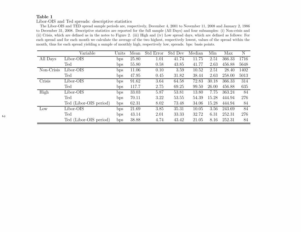
Table 1

Libor-OIS and Ted spreads: descriptive statisticsThe Libor-OIS and TED spread sample periods are, respectively, December 4, 2001 to November 11, 2008 and January 2, 1986

to December 31, 2008. Descriptive statistics are reported for the full sample (All Days) and four subsamples: (i) Non-crisis and(ii) Crisis, which are defined as in the notes to Figure 2. (iii) High and (iv) Low spread days, which are defined as follows: Foreach spread and for each month we calculate the average of the two highest, respectively lowest, values of the spread within themonth, thus for each spread yielding a sample of monthly high, respectively low, spreads. bps: basis points.

Variable Units Mean Std Error Std Dev Median Min Max NAll Days Libor-OIS bps 25.80 1.01 41.74 11.75 2.51 366.33 1716

Ted bps 55.80 0.58 43.85 41.77 2.63 456.88 5648Non-Crisis Libor-OIS bps 11.06 0.10 3.59 10.52 2.51 28.40 1402

Ted bps 47.95 0.45 31.82 38.44 2.63 258.00 5013Crisis Libor-OIS bps 91.62 3.64 64.58 72.83 30.18 366.33 314

Ted bps 117.7 2.75 69.25 99.50 26.00 456.88 635High Libor-OIS bps 33.03 5.87 53.81 13.80 7.75 363.24 84

Ted bps 70.11 3.22 53.55 54.39 15.28 444.94 276Ted (Libor-OIS period) bps 62.31 8.02 73.48 34.06 15.28 444.94 84

Low Libor-OIS bps 21.69 3.85 35.31 10.05 3.56 243.69 84Ted bps 43.14 2.01 33.33 32.72 6.31 252.31 276Ted (Libor-OIS period) bps 38.88 4.74 43.42 21.05 8.16 252.31 84

2

Table 2

Liquidity group transition matrixEach month, stocks are sorted into liquidity deciles (1 liquid and 10 illiquid), based on Amihud’s (2002)

ILLIQ [see equation (1) for the definition]. The table reports the percentage of stocks that are in group G onemonth and H the next; G, H = 1, . . . , 10.

month t + 1

month t

Group 1 2 3 4 5 6 7 8 9 101 89.88 9.76 0.19 0.08 0.04 0.02 0.01 0.01 0.01 0.012 9.84 72.69 16.41 0.85 0.14 0.05 0.02 0.01 0.00 0.003 0.23 15.61 61.07 20.36 2.21 0.39 0.09 0.02 0.01 0.004 0.05 1.00 18.35 53.43 22.72 3.53 0.73 0.15 0.03 0.015 0.02 0.20 2.49 19.82 48.46 23.12 4.68 0.98 0.19 0.046 0.01 0.06 0.50 3.61 19.90 45.88 23.52 5.33 1.02 0.187 0.00 0.02 0.14 0.88 4.58 20.14 44.32 23.54 5.59 0.808 0.01 0.00 0.04 0.24 1.18 5.25 20.39 44.20 24.33 4.359 0.01 0.00 0.02 0.06 0.27 1.22 5.33 21.58 48.14 23.3610 0.01 0.00 0.00 0.02 0.06 0.26 0.93 4.39 21.43 72.90

3

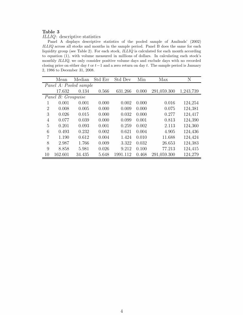
Table 3

ILLIQ : descriptive statisticsPanel A displays descriptive statistics of the pooled sample of Amihuds’ (2002)

ILLIQ across all stocks and months in the sample period. Panel B does the same for eachliquidity group (see Table 2). For each stock, ILLIQ is calculated for each month accordingto equation (1), with volume measured in millions of dollars. In calculating each stock’smonthly ILLIQ, we only consider positive volume days and exclude days with no recordedclosing price on either day t or t−1 and a zero return on day t. The sample period is January2, 1986 to December 31, 2008.

Mean Median Std Err Std Dev Min Max NPanel A: Pooled sample

17.632 0.134 0.566 631.266 0.000 291,059.300 1,243,739Panel B: Groupwise

1 0.001 0.001 0.000 0.002 0.000 0.016 124,2542 0.008 0.005 0.000 0.009 0.000 0.075 124,3813 0.026 0.015 0.000 0.032 0.000 0.277 124,4174 0.077 0.039 0.000 0.099 0.001 0.813 124,3905 0.201 0.093 0.001 0.259 0.002 2.113 124,3606 0.493 0.232 0.002 0.621 0.004 4.905 124,4367 1.190 0.612 0.004 1.424 0.010 11.688 124,4248 2.987 1.766 0.009 3.322 0.032 26.653 124,3839 8.858 5.981 0.026 9.212 0.100 77.213 124,415

10 162.601 34.435 5.648 1991.112 0.468 291,059.300 124,279

4

Table 4

Volume and returns by liquidity group on high versus low spread daysThis table presents sorts capturing the effect of spreads on stocks of different levels of liquidity. In the month prior to the observation month, all stocks are

sorted into ten groups based on ILLIQ (see Table 2), with Group 1 (10) consisting of the most (least) liquid stocks. The table reports average values of the selectedvariables on month-by-month high and low spread days for each liquidity group. In particular, for each spread and for each month, we select the two days withthe highest spreads and average the selected variables over these two days for each liquidity group. We do the same for the two lowest spread days. (If, for a givenmonth and spread, there are more than two highest (lowest) spread days, then we average across all those days. If there is a single highest (lowest) spread day andn second highest (lowest) spread days, we take a weighted average where the highest (lowest) spread day has a weight of 0.5 and the second highest (lowest) spreaddays have a weight of 0.5/n.) For each spread, each variable, and each liquidity group, this yields two time series with monthly observations on high and low spreaddays. The table reports the averages of these time series for each liquidity group. Panel A (B) classifies high and low spread days according to the Libor-OIS (TED)spread. The Libor-OIS and TED spread sample periods are, respectively, December 4, 2001 to November 11, 2008 and January 2, 1986 to December 31, 2008. a,b, and c denote statistical significance (two-tailed) at the 1%, 5%, and 10% level respectively. For all columns except Diff 1-10, statistical significance refers to thedifference between the variable on high and low spread days. In column Diff 1-10, a, b, and c indicate whether there is a statistically significant difference betweenGroups 1 and 10. Variables are defined in the appendix. Returns are daily and in percent.

Liquidity Group1 2 3 4 5 6 7 8 9 10 Diff 1-10 t-statistic

Panel A: Libor-OIS

HIGH

Normalized share volume 1.058b 1.052 1.056c 1.044 1.058 1.093 1.128 1.037 1.031 0.933a 0.125a 3.76Normalized dollar volume 1.054b 1.049 1.045 1.034 1.041 1.071 1.091 1.046 1.087 0.922b 0.132a 2.95Return (equally weighted) -0.048 -0.041 -0.073c -0.047c -0.081c -0.036c 0.016 -0.016c 0.019c 0.176c -0.225c -1.83LOW

Normalized share volume 0.999 1.010 1.012 1.028 1.030 1.053 1.035 1.037 1.060 1.090 -0.091b -2.34Normalized dollar volume 1.006 1.010 1.010 1.024 1.028 1.019 1.020 1.012 1.039 1.154 -0.148 -1.64Return (equally weighted) 0.176 0.204 0.237 0.240 0.242 0.267 0.244 0.203 0.234 0.328 -0.152 -1.26Panel B: Ted

HIGH

Normalized share volume 1.052a 1.041b 1.034c 1.032 1.038 1.034 1.04 1.028 1.036 0.997c 0.056a 3.22Normalized dollar volume 1.050a 1.040b 1.029 1.031 1.035 1.035 1.044 1.052c 1.036 1.004 0.046b 2.29Return (equally weighted) 0.004 0.002 -0.006 0.001 -0.013 -0.014 0.016 0.049 0.089 0.359 -0.355a -4.42LOW

Normalized share volume 1.004 1.012 1.009 1.014 1.016 1.024 1.013 1.021 1.024 1.033 -0.030c -1.72Normalized dollar volume 1.005 1.013 1.010 1.014 1.018 1.019 1.008 1.010 1.022 1.021 -0.016 -0.77Return (equally weighted) 0.107 0.126 0.132 0.135 0.133 0.138 0.109 0.120 0.163 0.369 -0.262a -4.14

5

Table 5

Differences in volume and returns between high and low spread daysFor each listed variable, this table reports the difference in its average value on high and low spread days, as reported in Table 4, for each liquidity group.

Panel A (B) classifies high and low spread days according to the Libor-OIS (TED) spread. The Libor-OIS and TED spread sample periods are, respectively,December 4, 2001 to November 11, 2008 and January 2, 1986 to December 31, 2008. a, b, and c denote statistical significance (two-tailed) at the 1%, 5%, and10% level respectively. For all columns except Diff 1-10, statistical significance refers to the difference between the variable on high and low spread days. Incolumn Diff 1-10, a, b, and c indicate whether there is a statistically significant difference between Groups 1 and 10. Variables are defined in the appendix.Returns are daily and in percent.

Liquidity Group1 2 3 4 5 6 7 8 9 10 Diff 1-10 t-statistic

Panel A: Libor-OIS

Normalized share volume 0.059b 0.042 0.044c 0.016 0.027 0.039 0.093 -0.001 -0.029 -0.157a 0.216a 4.04Normalized dollar volume 0.048b 0.039 0.035 0.010 0.012 0.052 0.071 0.034 0.047 -0.232b 0.280a 2.81Return (equally weighted) -0.224 -0.245 -0.310c -0.287c -0.323c -0.304c -0.228 -0.219c -0.215c -0.152c -0.072 -0.39Panel B: Ted

Normalized share volume 0.049a 0.029b 0.024c 0.017 0.022 0.011 0.027 0.007 0.012 -0.037 0.086a 3.28Normalized dollar volume 0.046a 0.027b 0.019 0.018 0.017 0.016 0.036 0.042c 0.014 -0.017 0.062b 2.03Return (equally weighted) -0.103 -0.124 -0.138 -0.133 -0.146 -0.152 -0.093 -0.071 -0.074 -0.01 -0.093 -0.976

Table 6

Fama-MacBeth regressions: Difference in normalized share volume on high versus lowspread days regressed on ILLIQ

Each month, m, we run the cross-sectional regressionHSVOLG,m − LSVOLG,m = αm + βm × ILLIQG,m−1 + εG,m.

We then report the average of all the cross-sectional coefficient estimates (αm, βm) with correspond-ing t-statistics. Standard errors are corrected using the Newey-West procedure with three lags.HSVOLG,m − LSVOLG,m is the difference in month m between the normalized share volumes onhigh versus low spread days for liquidity group G (see Tables 2 and 4). ILLIQG,m−1 is the equallyweighted average ILLIQ across stocks in liquidity group G in month m − 1. In specification (1) weuse the Libor-OIS spread to identify high and low spread days. Specification (2) uses the Ted spreadto identify high and low spread days. Specification (3) uses the Ted spread, but considers the timeperiod for which the Libor-OIS spread is available. Specifications (4) and (5) use the Libor-OIS andTed spread, respectively, but consider the period prior to the financial crisis (pre 07/2007). TheLibor-OIS and TED spread sample periods are, respectively, December 4, 2001 to November 11, 2008and January 2, 1986 to December 31, 2008. a, b, and c denote statistical significance (two-tailed)at the 1%, 5%, and 10% level respectively. Variables are defined in the appendix.

Spread / Period Intercept t-stat ILLIQG t-stat Adj. R2 N(1) Libor-OIS 0.034 (1.21) -0.015c (-1.80) 18.07% 83(2) Ted 0.023 (1.65) -0.004b (-2.28) 14.28% 275(3) Ted (OIS-period) 0.019 (0.66) -0.013b (-2.21) 20.30% 83(4) Libor-OIS (pre 07/2007) 0.026 (0.83) -0.017a (-2.79) 16.49% 66(5) Ted (pre 07/2007) 0.019 (1.50) -0.004b (-2.05) 13.70% 257

7

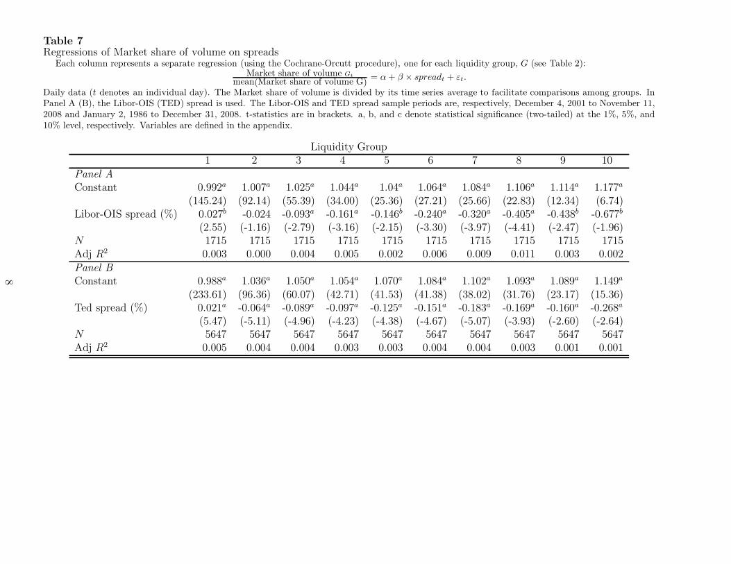
Table 7

Regressions of Market share of volume on spreadsEach column represents a separate regression (using the Cochrane-Orcutt procedure), one for each liquidity group, G (see Table 2):

Market share of volume Gt

mean(Market share of volume G)= α + β × spreadt + εt.

Daily data (t denotes an individual day). The Market share of volume is divided by its time series average to facilitate comparisons among groups. InPanel A (B), the Libor-OIS (TED) spread is used. The Libor-OIS and TED spread sample periods are, respectively, December 4, 2001 to November 11,2008 and January 2, 1986 to December 31, 2008. t-statistics are in brackets. a, b, and c denote statistical significance (two-tailed) at the 1%, 5%, and10% level, respectively. Variables are defined in the appendix.

Liquidity Group1 2 3 4 5 6 7 8 9 10

Panel A

Constant 0.992a 1.007a 1.025a 1.044a 1.04a 1.064a 1.084a 1.106a 1.114a 1.177a

(145.24) (92.14) (55.39) (34.00) (25.36) (27.21) (25.66) (22.83) (12.34) (6.74)Libor-OIS spread (%) 0.027b -0.024 -0.093a -0.161a -0.146b -0.240a -0.320a -0.405a -0.438b -0.677b

(2.55) (-1.16) (-2.79) (-3.16) (-2.15) (-3.30) (-3.97) (-4.41) (-2.47) (-1.96)N 1715 1715 1715 1715 1715 1715 1715 1715 1715 1715Adj R2 0.003 0.000 0.004 0.005 0.002 0.006 0.009 0.011 0.003 0.002Panel B

Constant 0.988a 1.036a 1.050a 1.054a 1.070a 1.084a 1.102a 1.093a 1.089a 1.149a

(233.61) (96.36) (60.07) (42.71) (41.53) (41.38) (38.02) (31.76) (23.17) (15.36)Ted spread (%) 0.021a -0.064a -0.089a -0.097a -0.125a -0.151a -0.183a -0.169a -0.160a -0.268a

(5.47) (-5.11) (-4.96) (-4.23) (-4.38) (-4.67) (-5.07) (-3.93) (-2.60) (-2.64)N 5647 5647 5647 5647 5647 5647 5647 5647 5647 5647Adj R2 0.005 0.004 0.004 0.003 0.003 0.004 0.004 0.003 0.001 0.001

8

Table 8

Libor-OIS, VIX, and control variables: descriptive statisticsPanel A is for the pre-crisis period, December 4, 2001 to July 29, 2007. Panel B is for the post TAF period, December 17, 2007 to November 11, 2008.

Daily data. Variables are defined in the appendix. TAF: term auction facility. bps: basis points.

Units Mean Std Error Std Dev Median Min Max N

Panel A: Pre-crisis period

Libor-OIS bps 11.09 0.10 3.60 10.60 2.51 28.40 1375

VIX % 17.73 0.19 6.92 15.50 9.89 45.08 1375

Group 1 Relative bid-ask % 12.36 0.16 5.78 10.58 4.95 39.18 1375

Group 2 Relative bid-ask % 16.83 0.17 6.32 14.91 7.72 44.32 1375

Group 3 Relative bid-ask % 21.26 0.16 5.98 19.44 11.58 45.91 1375

Group 4 Relative bid-ask % 27.51 0.16 6.12 25.74 16.07 51.02 1375

Group 5 Relative bid-ask % 36.82 0.20 7.42 35.60 20.43 59.11 1375

Group 6 Relative bid-ask % 53.81 0.26 9.69 52.76 32.78 82.47 1375

Group 7 Relative bid-ask % 84.26 0.30 10.98 82.05 63.99 113.70 1375

Group 8 Relative bid-ask % 134.81 0.25 9.12 134.09 106.24 165.03 1375

Group 9 Relative bid-ask % 216.05 0.31 11.58 216.55 173.99 265.59 1375

Group 10 Relative bid-ask % 396.30 1.19 44.18 408.97 280.52 485.78 1375

Lagmarket % 0.04 0.03 0.97 0.08 -3.82 5.32 1375

Normalized market dollar volume % 101.00 0.43 15.96 99.79 27.87 226.78 1375

Correlation between VIX and Libor-OIS 0.61

Panel B: Post-TAF period

Libor-OIS bps 100.48 4.91 73.68 73.93 30.18 366.33 225

VIX % 28.67 0.90 13.50 23.82 16.30 80.06 225

Group 1 Relative bid-ask % 8.78 0.19 2.79 8.49 4.07 27.78 225

Group 2 Relative bid-ask % 11.74 0.19 2.91 11.50 6.79 32.50 225

Group 3 Relative bid-ask % 13.44 0.20 2.93 13.36 8.39 36.63 225

Group 4 Relative bid-ask % 16.61 0.22 3.34 16.35 11.40 47.48 225

Group 5 Relative bid-ask % 22.13 0.29 4.36 21.82 14.06 62.22 225

Group 6 Relative bid-ask % 34.11 0.38 5.68 33.71 23.32 89.36 225

Group 7 Relative bid-ask % 65.33 0.59 8.89 63.70 50.45 134.35 225

Group 8 Relative bid-ask % 128.16 0.88 13.13 126.44 105.20 175.45 225

Group 9 Relative bid-ask % 228.54 1.07 16.07 225.76 190.79 274.56 225

Group 10 Relative bid-ask % 471.17 2.46 36.97 479.32 225.88 540.98 225

Lagmarket % -0.21 0.15 2.24 -0.06 -8.99 11.52 225

Normalized market dollar volume % 100.70 1.17 17.58 98.85 34.31 179.91 225

Correlation between VIX and Libor-OIS 0.89

9

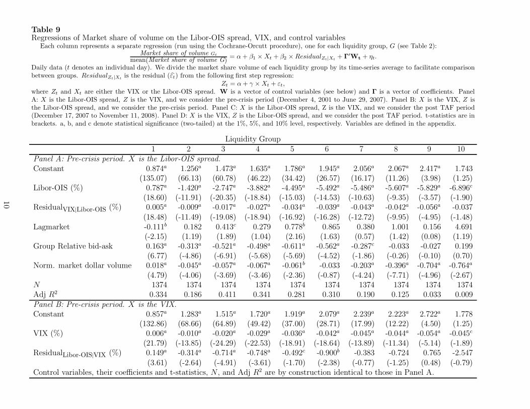
Table 9

Regressions of Market share of volume on the Libor-OIS spread, VIX, and control variablesEach column represents a separate regression (run using the Cochrane-Orcutt procedure), one for each liquidity group, G (see Table 2):

Market share of volume Gt

mean(Market share of volume G)= α + β1 × Xt + β2 × ResidualZt|Xt

+ Γ′Wt + ηt.

Daily data (t denotes an individual day). We divide the market share volume of each liquidity group by its time-series average to facilitate comparisonbetween groups. ResidualZt|Xt

is the residual (εt) from the following first step regression:Zt = α + γ × Xt + εt,

where Zt and Xt are either the VIX or the Libor-OIS spread. W is a vector of control variables (see below) and Γ is a vector of coefficients. PanelA: X is the Libor-OIS spread, Z is the VIX, and we consider the pre-crisis period (December 4, 2001 to June 29, 2007). Panel B: X is the VIX, Z isthe Libor-OIS spread, and we consider the pre-crisis period. Panel C: X is the Libor-OIS spread, Z is the VIX, and we consider the post TAF period(December 17, 2007 to November 11, 2008). Panel D: X is the VIX, Z is the Libor-OIS spread, and we consider the post TAF period. t-statistics are inbrackets. a, b, and c denote statistical significance (two-tailed) at the 1%, 5%, and 10% level, respectively. Variables are defined in the appendix.

Liquidity Group1 2 3 4 5 6 7 8 9 10

Panel A: Pre-crisis period. X is the Libor-OIS spread.

Constant 0.874a 1.256a 1.473a 1.635a 1.786a 1.945a 2.056a 2.067a 2.417a 1.743(135.07) (66.13) (60.78) (46.22) (34.42) (26.57) (16.17) (11.26) (3.98) (1.25)

Libor-OIS (%) 0.787a -1.420a -2.747a -3.882a -4.495a -5.492a -5.486a -5.607a -5.829a -6.896c

(18.60) (-11.91) (-20.35) (-18.84) (-15.03) (-14.53) (-10.63) (-9.35) (-3.57) (-1.90)ResidualVIX|Libor-OIS (%) 0.005a -0.009a -0.017a -0.027a -0.034a -0.039a -0.043a -0.042a -0.056a -0.037

(18.48) (-11.49) (-19.08) (-18.94) (-16.92) (-16.28) (-12.72) (-9.95) (-4.95) (-1.48)Lagmarket -0.111b 0.182 0.413c 0.279 0.778b 0.865 0.380 1.001 0.156 4.691

(-2.15) (1.19) (1.89) (1.04) (2.16) (1.63) (0.57) (1.42) (0.08) (1.19)Group Relative bid-ask 0.163a -0.313a -0.521a -0.498a -0.611a -0.562a -0.287c -0.033 -0.027 0.199

(6.77) (-4.86) (-6.91) (-5.68) (-5.69) (-4.52) (-1.86) (-0.26) (-0.10) (0.70)Norm. market dollar volume 0.018a -0.045a -0.057a -0.067a -0.061b -0.033 -0.203a -0.396a -0.704a -0.764a

(4.79) (-4.06) (-3.69) (-3.46) (-2.36) (-0.87) (-4.24) (-7.71) (-4.96) (-2.67)N 1374 1374 1374 1374 1374 1374 1374 1374 1374 1374Adj R2 0.334 0.186 0.411 0.341 0.281 0.310 0.190 0.125 0.033 0.009Panel B: Pre-crisis period. X is the VIX.

Constant 0.857a 1.283a 1.515a 1.720a 1.919a 2.079a 2.239a 2.223a 2.722a 1.778(132.86) (68.66) (64.89) (49.42) (37.00) (28.71) (17.99) (12.22) (4.50) (1.25)

VIX (%) 0.006a -0.010a -0.020a -0.029a -0.036a -0.042a -0.045a -0.044a -0.054a -0.045c

(21.79) (-13.85) (-24.29) (-22.53) (-18.91) (-18.64) (-13.89) (-11.34) (-5.14) (-1.89)ResidualLibor-OIS|VIX (%) 0.149a -0.314a -0.714a -0.748a -0.492c -0.900b -0.383 -0.724 0.765 -2.547

(3.61) (-2.64) (-4.91) (-3.61) (-1.70) (-2.38) (-0.77) (-1.25) (0.48) (-0.79)Control variables, their coefficients and t-statistics, N , and Adj R2 are by construction identical to those in Panel A.

10

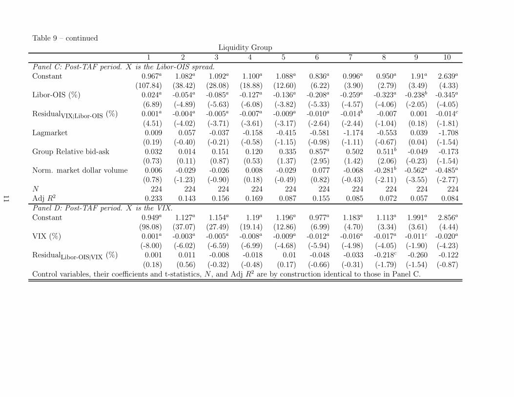
Table 9 – continuedLiquidity Group

1 2 3 4 5 6 7 8 9 10Panel C: Post-TAF period. X is the Libor-OIS spread.

Constant 0.967a 1.082a 1.092a 1.100a 1.088a 0.836a 0.996a 0.950a 1.91a 2.639a

(107.84) (38.42) (28.08) (18.88) (12.60) (6.22) (3.90) (2.79) (3.49) (4.33)Libor-OIS (%) 0.024a -0.054a -0.085a -0.127a -0.136a -0.208a -0.259a -0.323a -0.238b -0.345a

(6.89) (-4.89) (-5.63) (-6.08) (-3.82) (-5.33) (-4.57) (-4.06) (-2.05) (-4.05)ResidualVIX|Libor-OIS (%) 0.001a -0.004a -0.005a -0.007a -0.009a -0.010a -0.014b -0.007 0.001 -0.014c

(4.51) (-4.02) (-3.71) (-3.61) (-3.17) (-2.64) (-2.44) (-1.04) (0.18) (-1.81)Lagmarket 0.009 0.057 -0.037 -0.158 -0.415 -0.581 -1.174 -0.553 0.039 -1.708

(0.19) (-0.40) (-0.21) (-0.58) (-1.15) (-0.98) (-1.11) (-0.67) (0.04) (-1.54)Group Relative bid-ask 0.032 0.014 0.151 0.120 0.335 0.857a 0.502 0.511b -0.049 -0.173

(0.73) (0.11) (0.87) (0.53) (1.37) (2.95) (1.42) (2.06) (-0.23) (-1.54)Norm. market dollar volume 0.006 -0.029 -0.026 0.008 -0.029 0.077 -0.068 -0.281b -0.562a -0.485a

(0.78) (-1.23) (-0.90) (0.18) (-0.49) (0.82) (-0.43) (-2.11) (-3.55) (-2.77)N 224 224 224 224 224 224 224 224 224 224Adj R2 0.233 0.143 0.156 0.169 0.087 0.155 0.085 0.072 0.057 0.084Panel D: Post-TAF period. X is the VIX.

Constant 0.949a 1.127a 1.154a 1.19a 1.196a 0.977a 1.183a 1.113a 1.991a 2.856a

(98.08) (37.07) (27.49) (19.14) (12.86) (6.99) (4.70) (3.34) (3.61) (4.44)VIX (%) 0.001a -0.003a -0.005a -0.008a -0.009a -0.012a -0.016a -0.017a -0.011c -0.020a

(-8.00) (-6.02) (-6.59) (-6.99) (-4.68) (-5.94) (-4.98) (-4.05) (-1.90) (-4.23)ResidualLibor-OIS|VIX (%) 0.001 0.011 -0.008 -0.018 0.01 -0.048 -0.033 -0.218c -0.260 -0.122

(0.18) (0.56) (-0.32) (-0.48) (0.17) (-0.66) (-0.31) (-1.79) (-1.54) (-0.87)Control variables, their coefficients and t-statistics, N , and Adj R2 are by construction identical to those in Panel C.

11

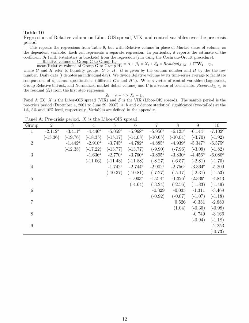
Table 10

Regressions of Relative volume on Libor-OIS spread, VIX, and control variables over the pre-crisisperiod

This repeats the regressions from Table 9, but with Relative volume in place of Market share of volume, asthe dependent variable. Each cell represents a separate regression. In particular, it reports the estimate of thecoefficient β1 (with t-statistics in brackets) from the regression (run using the Cochrane-Orcutt procedure):

Relative volume of Group G to Group Ht

mean(Relative volume of Group G to Group H)= α + β1 × Xt + β2 × ResidualZt|Xt

+ Γ′Wt + ηt,

where G and H refer to liquidity groups, G > H . G is given by the column number and H by the the rownumber. Daily data (t denotes an individual day). We divide Relative volume by its time-series average to facilitate

comparisons of β1 across specifications (different G’s and H ’s). W is a vector of control variables (Lagmarket,Group Relative bid-ask, and Normalized market dollar volume) and Γ is a vector of coefficients. ResidualZt|Xt

isthe residual (εt) from the first step regression:

Zt = α + γ × Xt + εt.Panel A (B): X is the Libor-OIS spread (VIX) and Z is the VIX (Libor-OIS spread). The sample period is thepre-crisis period (December 4, 2001 to June 29, 2007). a, b and c denote statistical significance (two-tailed) at the1%, 5% and 10% level, respectively. Variables are defined in the appendix.

Panel A: Pre-crisis period. X is the Libor-OIS spread.Group 2 3 4 5 6 7 8 9 10

1 -2.112a -3.411a -4.446a -5.059a -5.968a -5.956a -6.125a -6.144a -7.102c

(-13.36) (-19.76) (-18.35) (-15.17) (-14.08) (-10.65) (-10.04) (-3.70) (-1.92)2 -1.442a -2.910a -3.745a -4.782a -4.885a -4.939a -5.347a -6.575c

(-12.38) (-17.22) (-13.77) (-13.77) (-9.90) (-7.96) (-3.09) (-1.82)3 -1.636a -2.770a -3.760a -3.895a -3.830a -4.456a -6.080c

(-11.06) (-11.43) (-11.88) (-8.27) (-6.57) (-2.81) (-1.70)4 -1.742a -2.744a -2.902a -2.756a -3.364b -5.209

(-10.37) (-10.81) (-7.27) (-5.17) (-2.31) (-1.53)5 -1.003a -1.214a -1.326b -2.339c -4.843

(-4.64) (-3.24) (-2.56) (-1.83) (-1.49)6 -0.329 -0.035 -1.311 -3.469

(-0.92) (-0.07) (-1.07) (-1.18)7 0.526 -0.331 -2.880

(1.04) (-0.30) (-0.98)8 -0.749 -3.166

(-0.94) (-1.18)9 -2.253

(-0.73)

12

Table 10 – continued

Panel B: Pre-crisis period. X is the VIX.Group 2 3 4 5 6 7 8 9 10

1 -0.015a -0.024a -0.033a -0.039a -0.044a -0.047a -0.048a -0.056a -0.046c

(-15.46) (-23.29) (-21.79) (-19.15) (-18.05) (-13.80) (-12.33) (-5.28) (-1.88)2 -0.011a -0.023a -0.030a -0.038a -0.041a -0.038a -0.050a -0.044c

(-15.59) (-22.47) (-17.85) (-17.97) (-13.36) (-9.52) (-4.51) (-1.86)3 -0.014a -0.023a -0.031a -0.035a -0.031a -0.044a -0.042c

(-15.59) (-15.40) (-15.77) (-11.64) (-8.14) (-4.26) (-1.80)4 -0.014a -0.022a -0.027a -0.024a -0.036a -0.036

(-14.73) (-14.68) (-11.17) (-7.04) (-3.87) (-1.60)5 -0.008a -0.015a -0.012a -0.026a -0.032

(-6.63) (-6.46) (-3.74) (-3.16) (-1.50)6 -0.009a -0.004 -0.018b -0.025

(-3.95) (-1.22) (-2.23) (-1.29)7 0.003 -0.01 -0.019

(1.04) (-1.35) (-1.00)8 -0.011b -0.020

(-2.24) (-1.14)9 -0.010

(-0.47)

13

Table 11

Regressions of Market share of volume on the Libor-OIS spread, VIX, and control variables: NASDAQ stocks excludedThis table runs the same regressions as in Table 9, Panels A and B, but with NASDAQ stocks excluded from the whole analysis. Each column

represents a separate regression (run using the Cochrane-Orcutt procedure), one for each liquidity group, G (see Table 2):Market share of volume Group G

t

mean(Market share of volume Group G)= α + β1 × Xt + β2 × ResidualZt|Xt

+ Γ′Wt + ηt.

Daily data (t denotes an individual day). We divide the market share volume of each liquidity group by its time-series average to facilitate comparisonbetween groups. ResidualZt|Xt

is the residual (εt) from the following first step regression:Zt = α + γ × Xt + εt,

where Zt and Xt are either the VIX or the Libor-OIS spread. W is a column vector of control variables and Γ is a row vector of coefficients. Panel A:X is the Libor-OIS spread, Z is the VIX, and we consider the pre-crisis period (December 4, 2001 to June 29, 2007). Panel B: X is the VIX, Z is theLibor-OIS spread, and we consider the pre-crisis period. Panel C: X is the Libor-OIS spread, Z is the VIX, we consider the post TAF period (December17, 2007 to November 11, 2008). Panel D: X is the VIX, Z is the Libor-OIS spread, and we consider the post TAF period. t-statistics are in brackets.a, b, and c denote statistical significance (two-tailed) at the 1%, 5%, and 10% level, respectively. Variables are defined in the appendix.

Liquidity Group1 2 3 4 5 6 7 8 9 10

Panel A: Pre-crisis period. X is the Libor-OIS spread.

Constant 0.844a 1.119a 1.299a 1.399a 1.511a 1.582a 1.805a 1.725a 2.018a 1.480a

(113.28) (79.99) (63.15) (57.37) (47.07) (35.55) (30.15) (19.07) (15.66) (3.70)Libor-OIS (%) 0.905a -0.693a -1.525a -2.461a -3.067a -4.335a -5.363a -5.015a -4.338a -2.816b

(18.62) (-8.40) (-11.62) (-15.88) (-15.26) (-15.02) (-16.47) (-12.73) (-8.99) (-2.20)ResidualVIX|Libor-OIS (%) 0.005a -0.003a -0.008a -0.016a -0.021a -0.026a -0.034a -0.04a -0.038a -0.037a

(16.28) (-6.35) (-9.19) (-15.12) (-15.14) (-13.04) (-15.45) (-14.78) (-11.44) (-4.31)Lagmarket -0.056 -0.079 0.309 0.180 0.221 0.342 0.407 0.210 -1.118c 1.922

(-0.81) (-0.51) (1.59) (0.79) (0.79) (1.05) (0.94) (0.39) (-1.65) (1.10)Group Relative bid-ask 0.163a -0.010 -0.248a -0.189a -0.178a -0.067c -0.145a -0.006 -0.053 0.137c

(6.66) (-0.32) (-5.73) (-4.77) (-4.19) (-1.72) (-2.84) (-0.11) (-1.10) (1.83)Norm. market dollar volume 0.035a -0.040a -0.072a -0.069a -0.103a -0.064a -0.089a -0.158a -0.421a -0.703a

(7.36) (-3.88) (-5.41) (-4.46) (-5.34) (-2.83) (-2.97) (-4.25) (-9.04) (-5.86)N 1374 1374 1374 1374 1374 1374 1374 1374 1374 1374Adj R2 0.346 0.083 0.196 0.278 0.248 0.175 0.237 0.176 0.146 0.048Panel B: Pre-crisis period. X is the VIX.

Constant 0.833a 1.120a 1.308a 1.443a 1.574a 1.638a 1.894a 1.898a 2.203a 1.738a

(113.64) (83.13) (65.39) (60.58) (49.60) (35.82) (31.66) (20.80) (17.23) (4.27)VIX (%) 0.006a -0.004a -0.010a -0.018a -0.023a -0.030a -0.039a -0.041a -0.038a -0.032a

(20.64) (-9.03) (-12.27) (-18.56) (-18.18) (-15.90) (-18.85) (-16.67) (-12.53) (-3.99)ResidualLibor-OIS|VIX (%) 0.268a -0.283a -0.549a -0.577a -0.625a -1.247a -1.320a -0.294 0.125 1.544

(5.45) (-3.15) (-4.09) (-3.63) (-3.07) (-4.72) (-4.07) (-0.73) (0.25) (1.25)Control variables, their coefficients and t-statistics, N , and Adj R2 are by construction identical to those in Panel A.

14

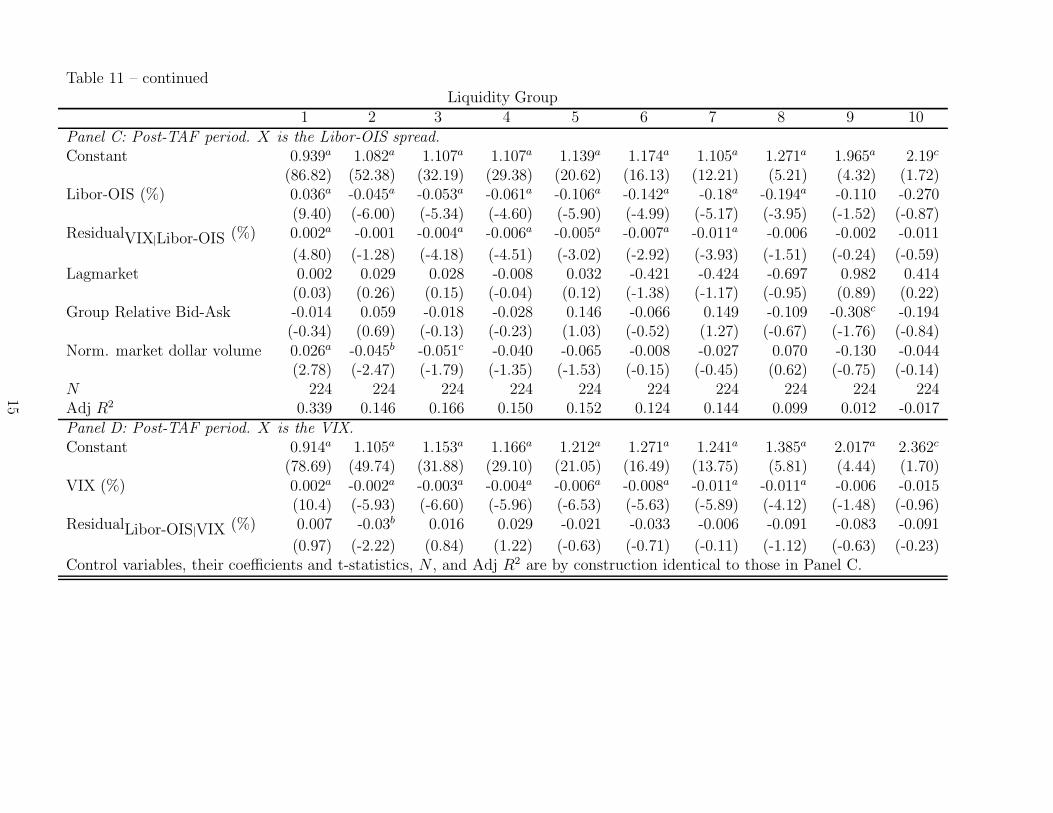
Table 11 – continuedLiquidity Group

1 2 3 4 5 6 7 8 9 10Panel C: Post-TAF period. X is the Libor-OIS spread.

Constant 0.939a 1.082a 1.107a 1.107a 1.139a 1.174a 1.105a 1.271a 1.965a 2.19c

(86.82) (52.38) (32.19) (29.38) (20.62) (16.13) (12.21) (5.21) (4.32) (1.72)Libor-OIS (%) 0.036a -0.045a -0.053a -0.061a -0.106a -0.142a -0.18a -0.194a -0.110 -0.270

(9.40) (-6.00) (-5.34) (-4.60) (-5.90) (-4.99) (-5.17) (-3.95) (-1.52) (-0.87)ResidualVIX|Libor-OIS (%) 0.002a -0.001 -0.004a -0.006a -0.005a -0.007a -0.011a -0.006 -0.002 -0.011

(4.80) (-1.28) (-4.18) (-4.51) (-3.02) (-2.92) (-3.93) (-1.51) (-0.24) (-0.59)Lagmarket 0.002 0.029 0.028 -0.008 0.032 -0.421 -0.424 -0.697 0.982 0.414

(0.03) (0.26) (0.15) (-0.04) (0.12) (-1.38) (-1.17) (-0.95) (0.89) (0.22)Group Relative Bid-Ask -0.014 0.059 -0.018 -0.028 0.146 -0.066 0.149 -0.109 -0.308c -0.194

(-0.34) (0.69) (-0.13) (-0.23) (1.03) (-0.52) (1.27) (-0.67) (-1.76) (-0.84)Norm. market dollar volume 0.026a -0.045b -0.051c -0.040 -0.065 -0.008 -0.027 0.070 -0.130 -0.044

(2.78) (-2.47) (-1.79) (-1.35) (-1.53) (-0.15) (-0.45) (0.62) (-0.75) (-0.14)N 224 224 224 224 224 224 224 224 224 224Adj R2 0.339 0.146 0.166 0.150 0.152 0.124 0.144 0.099 0.012 -0.017Panel D: Post-TAF period. X is the VIX.

Constant 0.914a 1.105a 1.153a 1.166a 1.212a 1.271a 1.241a 1.385a 2.017a 2.362c

(78.69) (49.74) (31.88) (29.10) (21.05) (16.49) (13.75) (5.81) (4.44) (1.70)VIX (%) 0.002a -0.002a -0.003a -0.004a -0.006a -0.008a -0.011a -0.011a -0.006 -0.015

(10.4) (-5.93) (-6.60) (-5.96) (-6.53) (-5.63) (-5.89) (-4.12) (-1.48) (-0.96)ResidualLibor-OIS|VIX (%) 0.007 -0.03b 0.016 0.029 -0.021 -0.033 -0.006 -0.091 -0.083 -0.091

(0.97) (-2.22) (0.84) (1.22) (-0.63) (-0.71) (-0.11) (-1.12) (-0.63) (-0.23)Control variables, their coefficients and t-statistics, N , and Adj R2 are by construction identical to those in Panel C.

15