Monetary persistence and the labor market: A new perspective

Monetary Persistence and the Labor Market: A New Perspective

Wolfgang Lechthaler Christian Merkl

Dennis J. Snower

CESIFO WORKING PAPER NO. 2935 CATEGORY 7: MONETARY POLICY AND INTERNATIONAL FINANCE

JANUARY 2010

An electronic version of the paper may be downloaded • from the SSRN website: www.SSRN.com • from the RePEc website: www.RePEc.org

• from the CESifo website: Twww.CESifo-group.org/wp T

CESifo Working Paper No. 2935

Monetary Persistence and the Labor Market: A New Perspective

Abstract In this paper we propose a novel way to model the labor market in the context of a New-Keynesian general equilibrium model, incorporating labor market frictions in the form of hiring and firing costs. We show that such a model is able to replicate many important stylized facts of the business cycle. The reactions to monetary and real shocks become much more sluggish. Job creation and job destruction are negatively correlated. And the volatility of unemployment is much larger than in the standard search and matching model.

JEL-Code: A00, A10, A11, E24, E32, E52, J23.

Keywords: monetary persistence, labor market, hiring and firing costs.

Wolfgang Lechthaler Kiel Institute for the World Economy

Düsternbrookerweg 120 Germany – 24105 Kiel

[email protected]

Christian Merkl Kiel Institute for the World Economy

Düsternbrookerweg 120 Germany – 24105 Kiel

[email protected]

Dennis J. Snower Kiel Institute for the World Economy

Düsternbrookerweg 120 Germany – 24105 Kiel [email protected]

1 Introduction

This paper offers a novel approach of integrating labor market frictions into astandard New Keynesian model with sticky prices. The labor market frictionshelp explain (i) output and unemployment persistence in response to real andmonetary shocks, (ii) strong amplification effects of real and monetary shockson unemployment and the job finding rate, and (iii) the negative correlationbetween job creation and job destruction.

At the beginning of each period, unemployed workers choose randomly oneof the firms and apply for a job. Worker-firm specific pairs are subject toidiosyncratic shocks. In addition, firms face linear hiring and firing costs. Thesesimple assumptions are sufficient to replicate several important business cyclefacts.

First, our model generates output and unemployment persistence in reactionto monetary and real shocks and inflation persistence in response to real shocks.Labor turnover costs - which in this paper are represented by linear hiring andfiring costs - lead to a sluggish adjustment in the labor market, even afterthe monetary impulse or the productivity shock have disappeared. Since laborturnover costs reduce the hiring and firing rates by making hiring and firingmore costly, they reduce the levels of hiring and firing activity in the aftermathof a monetary shock. Sluggish labor market adjustment also leads to sluggishproduct market adjustment after a shock - more sluggish than in the standardNew Keynesian models and in closer agreement with the empirical evidence.

Second, the labor market variables in the model show a strong amplificationeffect in response to both monetary and real shocks. In line with empiricalevidence, the standard deviation of the job-finding rate and the unemploymentis several times larger than the standard deviation of output. The reason is thatidiosyncratic shocks play an important role for the creation of new jobs in ourmodel.1

Third, our model is able to replicate a negative correlation between thejob-finding rate and unemployment. Further, it generates a strong negativecorrelation between job creation and the job destruction.2

It is well known that the standard small-scale New Keynesian frameworkwith a representative household and neoclassical labor markets does not gen-erate any monetary persistence when the central bank deviates in uncorrelatedmanner from the Taylor rule interest rate behavior. To overcome this prob-lem, medium scale DSGE models (e.g., Christiano et al., 2005, or Smets andWouters, 2003, 2007) contain several assumptions which may be difficult to rec-oncile with microeconomic evidence (e.g., habit formation3 or backward-looking

1In contrast, in the standard calibration of search and matching models, the idiosyncraticproductivity shock is set to replicate the appropriate job destruction rate, while it plays onlya minor role for job creation, which is primarily driven by the matching function. See Section5 for a more detailed intuitive explanation.

2search and matching models with endogenous separations and flexible wages are unableto do so. See Krause and Lubik, 2007.

3Habit formation may be present for specific goods or services, but not for the entireconsumption bundle, as it is generally assumed in medium scale models.

1

indexation4).Recently, the interaction of imperfect labor markets and labor adjustment

costs with business cycle dynamics has drawn a lot of attention. Campbelland Fisher, 2000, analyze how hiring and firing costs affect job-turnover at thefirm and industry level. Veracierto, 2008, shows in a model of employmentlotteries that firing restrictions reduce business cycle fluctuations. In addition,there are several recent contributions that include search and matching frictionsinto the New Keynesian model (e.g., Walsh, 2005, Blanchard and Galı, 2010,Christoffel and Linzert, 2006, Faia, 2008, Krause and Lubik, 2007, Thomas,2008, Barnichon, 2008).

As noted by Costain and Reiter, 2008, and Shimer, 2005, the standard searchand matching model is not able to replicate the large volatilities of unemploy-ment found in the data. There have been various attempts to remedy thisproblem. Hall, 2005, introduces wage rigidity. Hagedorn and Manovskii, 2008,propose an alternative calibration, using a very high value of unemployment,which implies that workers do not gain much from finding a job. They notethat this is especially relevant for short-term unemployed people. Thus, theircalibration obviously fits better to the US than to European countries with theircomparably low job-finding rates. Cooper et al., 2005, build a very rich modelwith fixed and variable costs of hirings, adjustments on the intensive marginand autocorrelated firm-specific shocks. To be able to handle the complexityof the model, they deviate from the common assumption of wage negotiationsand assume that firms can set the wage in a take-it-or-leave-it manner. Weoffer an alternative avenue of bringing the predictions of the new Keynesianmodel into closer consonance with the empirical evidence, namely, by introduc-ing labor market frictions in the form of hiring and firing costs and providing anew analysis of labor market flows. The assumption of perfect labor markets iswidely considered to be a conspicuous weakness of the standard new Keynesianmodels and this paper shows how this weakness may be addressed in a simpleand tractable way and how doing so helps explain various well-know stylizedfacts.

Our analysis examines the influence of hiring and firing costs on the ef-fectiveness of monetary policy.5 These labor market rigidities are empiricallyobservable6 and the monetary policy transmission mechanism can be given astraightforward intuition on this basis.

In the absence of labor turnover costs, a worker’s current employment prob-ability is independent of whether she was previously employed or unemployed,so that her retention rate is equal to her job finding rate. In the presence of hir-ing and firing costs, by contrast, her retention rate exceeds her job finding rate,

4There is little empirical microeconomic evidence for such indexation. See Woodford, 2007,for a discussion of this issue.

5Rotemberg and Woodford, 1999, analyze convex labor adjustment costs. But they focussolely on the implications of these costs for fluctuations of the markup over the business-cycle.Furthermore, their approach does not allow for unemployment.

6For the analysis and quantification of firing costs, see, for example, Botero et al., 2004,OECD, 2004, and World Bank, 2008.

2

and thus current employment depends on past employment. In this setting, acurrent monetary shock affects not only current, but also future employment.Since labor is used to produce output, employment persistence is translated intooutput persistence.

Specifically, in the presence of a positive, temporary macroeconomic shock,workers are hired but, on account of firing costs, these workers are not promptlydismissed as soon as the shock is over. Thus, the effects of the shock on em-ployment and output persist. But even in the absence of firing costs, hiringcosts create employment and output persistence. For instance, once a tempo-rary positive shock has passed, some workers are retained who would not havebeen hired in the absence of this shock, due to hiring costs. Thus the positiveshock has persistent after-effects.7 In this way, the inclusion of labor turnovercosts can be shown to explain how monetary shocks have prolonged effects onoutput and employment.

We calibrate our model under realistic values of hiring and firing costs fora typical European economy. Under uncorrelated iid monetary shocks, it takesseveral quarters until the economy returns to the steady state, while the stan-dard model generates no persistence at all. After autocorrelated productivityshocks, employment, output and inflation show hump-shaped responses. Thuslabor adjustment costs offer a new explanation for output persistence, whichhas so far been largely unexplored.

The rest of the paper is structured as follows. Section 2 presents the the-oretical model and Section 3 explains the calibration. Section 4 discusses themodel outcomes, while Section 5 illustrates important business cycle statistics.Section 6 concludes.

2 The Model

Our model grafts a labor market with labor turnover costs, wage bargaining,and employed and unemployed workers onto a New Keynesian framework withRotemberg adjustment costs. To endogenize hiring and firing decisions, it isassumed that the profitability of each worker is subject to an iid shock eachperiod. Firms can change their price in any period but price changes are subjectto quadratic adjustment costs. Monetary policy is represented by a Taylor rule.

2.1 Households

We assume that households have a standard utility function of the form:8

7Alternatively, consider an employee whose productivity is just high enough to be retained.An unemployed worker with the same productivity will not be offered a job, however, due tothe positive hiring cost. In short, hiring costs create persistence in the aftermath of a shock,because in the presence of hiring costs, the retention probability of employees exceeds thehiring probability of the unemployed.

8This is similar to the utility function in Krause and Lubik, 2007, except that we do notneed money in the utility function, since we model monetary policy by a Taylor rule ratherthan by a money growth rule.

3

Ut = Et

∞∑

j=t

βj−tc1−σj

1− σ, (1)

where β is the household’s discount factor, σ the elasticity of intertemporalsubstitution, c a consumption aggregate (described below)9 and E is the expec-tation operator.

As is common in the literature, we assume that each household consists of alarge number of individuals, each individual supplies one unit of labor inelasti-cally and shares all income with the other household members (see, e.g., Merz,1995 or Andolfatto, 1996). This implies that consumption does not depend ona worker’s employment status. Thus, the representative household maximizesits utility subject to the budget constraint:

Bot + ctPt = WtNt +BUt + (1 + it−1)Bot−1 +Πa,t − Tt, (2)

where Bo are nominal bond holdings, P is the aggregate price level, T are taxpayments, i is the nominal interest rate and Πa are nominal aggregate profits,which are transferred in lump-sum manner, W is the nominal wage, N is thetotal household labor input, B the income of unemployed workers10 and U thenumber of unemployed workers. The intertemporal utility maximization yieldsthe standard consumption Euler equation:

ct = βEtct+1

((1 + it)

Pt

Pt+1

)− 1σ

. (3)

2.2 Production and the Labor Market

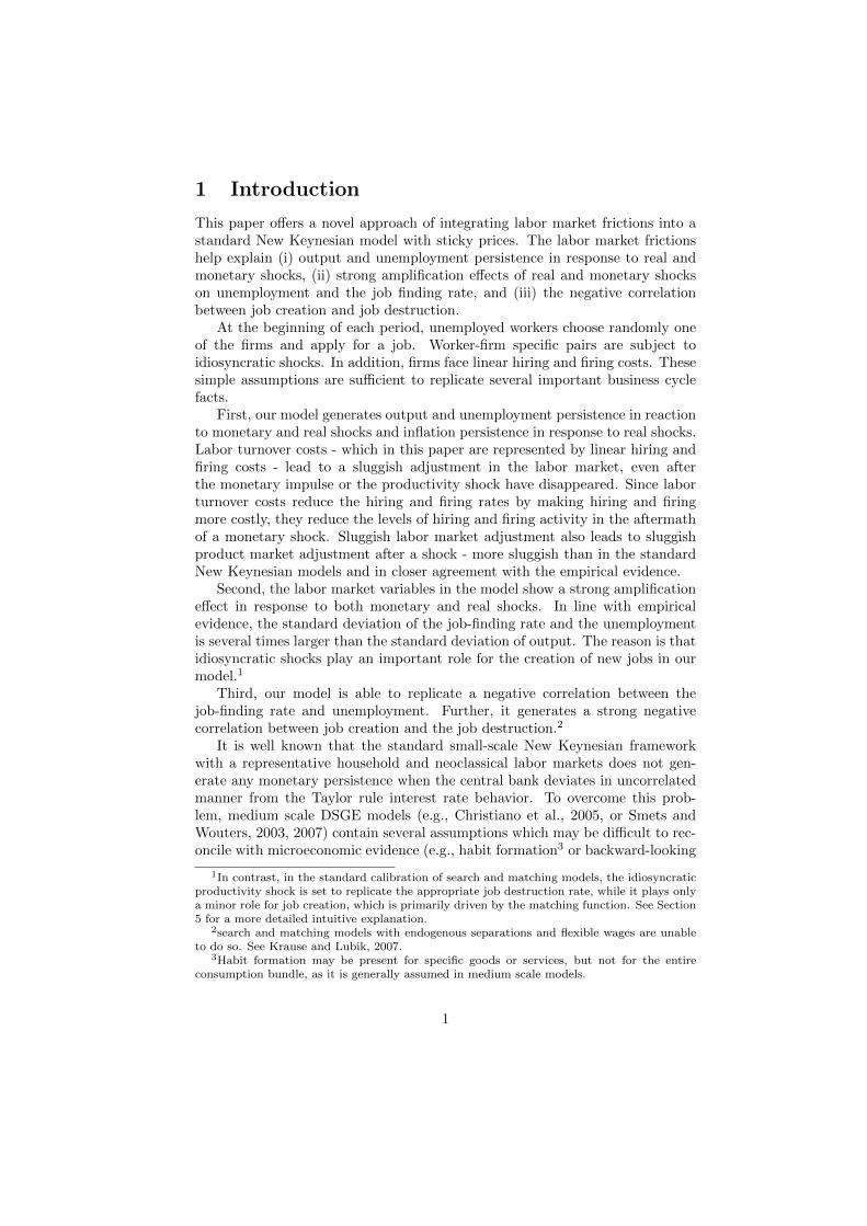
There are three types of firms. (i) Firms that produce intermediate goodsemploy labor, exhibit linear labor adjustment costs (i.e., hiring and firing costs)and sell their homogenous products on a perfectly competitive market to thewholesale sector. (ii) Firms in the wholesale sector transform the intermediategoods into consumption goods and sell them under monopolistic competition tothe retailers. They can change their price at any time but price adjustments aresubject to a quadratic adjustment cost a la Rotemberg. (iii) The retailers, inturn, aggregate the consumption goods and sell them under perfect competitionto the households. The structure of the model is illustrated in Figure 1.

2.2.1 Intermediate Goods Producers

Intermediate good firms hire labor to produce the intermediate good z. Theirproduction function is:

9In what follows capital letters refer to nominal variables and small letters refer to realvariables (i.e., detrended by the price level).

10B can either be interpreted as home production or as unemployment benefits provided bythe government (financed by lump-sum taxes).

4

Intermediate

Goods

ProducersHouseholds

Labor Market withUnemployment

Stylized Model Structure

Wholesale

Sector

Central Bank

ConsumptionGoods

Retail SectorBundled Good

Intermediate Good Labor

Bonds / M

oney

Rotemberg

Wage BargainingPerfect

Competition

AdjustmentCosts

Taylo

r Rule

Figure 1: Model structure

zt = atNt, (4)

where a is technology and N the number of employed workers. They sell theproduct at a relative price pz,t = Pz,t/Pt, which they take as given in a perfectlycompetitive environment, where Pz is the absolute price of the intermediate goodand P is the economy’s overall price level.

The labor market approach follows Snower and Merkl, 2006, and Brown,Merkl and Snower, 2007, who model the labor market in a pure partial equilib-rium setting, while we extend it to a general equilibrium setting.11

We assume an economy with a large number of firms and a large number ofworkers. At the beginning of each period, unemployed workers choose randomlyone of the firms and apply for a job there. For the resulting worker-firm pair, anidiosyncratic operating cost, εt, is drawn, e.g., during the subsequent interviewthe mutual fit is revealed. The operating costs are measured in terms of the finalconsumption good. If the shock is sufficiently bad, no match will be made, theworker stays unemployed this period and will contact an other firm next period.Employed workers are also hit by a shock, drawn from the same distribution.

The firms learn the value of the operating costs of every worker at the begin-ning of a period and base their employment decisions on it, i.e., an unemployedworker with a favorable shock will be employed while an employed worker with abad shock will be fired. Hiring and firing is not costless, firms have to pay linearhiring costs, h, and linear firing costs, f , both measured in terms of the finalconsumption good. Wages are determined by bargaining between the medianworker and the firm.

11The approach is similar to the way that separations are endogenized in search and match-ing models, see Mortensen and Pissarides, 1999.

5

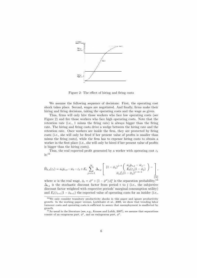
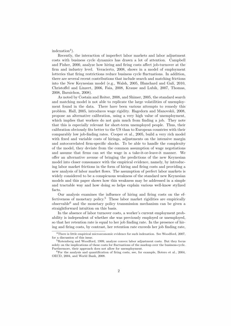
Figure 2: The effect of hiring and firing costs

We assume the following sequence of decisions: First, the operating costshock takes place. Second, wages are negotiated. And finally, firms make theirhiring and firing decisions, taking the operating costs and the wage as given.

Thus, firms will only hire those workers who face low operating costs (seeFigure 2) and fire those workers who face high operating costs. Note that theretention rate (i.e., 1 minus the firing rate) is always bigger than the firingrate. The hiring and firing costs drive a wedge between the hiring rate and theretention rate. Once workers are inside the firm, they are protected by firingcosts (i.e., she will only be fired if her present value of profits is smaller thanminus the firing costs), while the firm has to expense hiring costs to obtain aworker in the first place (i.e., she will only be hired if her present value of profitsis bigger than the hiring costs).

Thus, the real expected profit generated by a worker with operating cost εtis:12

ΠI,t(εt) = atpz,t−wt−εt+Et

∞∑

j=t+1

∆t,j

(1− φj)

j−t

(ajpz,j − wj−Et(εj |1− φj)

)−

φjfj(1− φj)j−t−1

,

(5)where w is the real wage, φt = φx + (1− φx)φn

t is the separation probability,13

∆t,j is the stochastic discount factor from period t to j (i.e., the subjectivediscount factor weighted with respective periods’ marginal consumption utility)and Et(εt+1|1− φt+1) the expected value of operating costs for an insider (i.e.,

12We only consider transitory productivity shocks in this paper and ignore productivitygrowth. In the working paper version, Lechthaler et al., 2008, we show that trending laborturnover costs and operating costs is sufficient to assure that unemployment is unaffected bygrowth.

13As usual in the literature (see, e.g., Krause and Lubik, 2007), we assume that separationsconsist of an exogenous part, φx, and an endogenous part, φn.

6

conditional on retention), given by:

Et(εt+1|1− φt+1) = Et

(1

1− φt+1

∫ υf

−∞εt+1g(εt+1)dεt+1

). (6)

where g(εt) is the probability density function of the operating cost. To simplifythe profit function, we rewrite it in recursive manner:

ΠI,t = atpz,t − wt − εt + Et(∆t,t+1ΠI,t+1), (7)

where Et(ΠI,t+1) are expected future profits, defined as:

Et(ΠI,t+1) = Et

((1− φt+1)(pz,t+1at+1 − wt+1 − Et(εt+1|1− φt+1))

+(1− φt+1)∆t,t+1ΠI,t+2 − φt+1f

). (8)

Unemployed workers are hired whenever their operating cost does not exceeda certain threshold such that the profitability of this worker is higher than thehiring cost (see Figure 2 for the graphical illustration), i.e., ΠI,t(εt) > h. Thus,the hiring threshold υh,t (the value of the operating cost at which the firm isindifferent between hiring and not hiring an unemployed worker) is defined by:

ΠI,t(υh,t) = atpz,t − wt − υh,t + Et(∆t,t+1ΠI,t+1) = h. (9)

Unemployed workers whose operating cost is lower than this value get a job,while those whose operating cost is higher remain unemployed. The resultinghiring probability is given by:

ηt = Γ(υh,t), (10)

where Γ is the cumulative density function of ε. Similarly, the firm will firea worker whenever ΠI,t(εt) < −f , i.e., when the operating costs are so highthat it is more profitable for the firm to pay the firing cost. This defines thefiring threshold (the value of the operating cost at which the firm is indifferentbetween firing and retaining the worker) as

ΠI,t(υf,t) = atpz,t − wt − υf,t + Et(∆t,t+1ΠI,t+1) = −f , (11)

and the rate of endogenous job destruction is given by

φnt = 1− Γ(υf,t). (12)

2.2.2 Employment

The change in employment (Nt −Nt−1) is the difference between the hiringfrom the unemployment pool (ηUt−1) and the firing from the employment pool(φNt−1), where Ut−1 and Nt−1 are the aggregate unemployment and employ-ment levels: Nt − Nt−1 = ηUt−1 − φNt−1. Letting (nt = Nt/Lt) be the em-ployment rate, we assume a constant workforce, Lt, and normalize it to one.Thereby, we obtain the following employment dynamics curve.

7

nt = nt−1(1− φt − ηt) + ηt. (13)

The unemployment rate is simply ut = 1− nt.

2.2.3 Wage Bargaining

We assume that wages are bargained between the firm and its median worker.This assumption fits especially well to the unionized labor markets of continentalEurope, but even in the US many industries are influenced by trade unions.14

In analogy to Hall and Milgrom, 2008, and Snower and Merkl, 2006, we assumethat the fall-back position is to continue negotiations next period.15 To highlightthat our results are driven by labor turnover costs, the wage is calibrated in sucha way that it responds strongly to changes in average productivity.

The wage is renegotiated in each period t. Under bargaining agreement,the worker receives the real wage wt and the firm receives the expected profit(atpz,t − wt − ε), where ε is the operating cost of the median worker. Underdisagreement, the worker’s fallback income is b, assumed for simplicity to beequal to real unemployment benefits.16 The firm’s fallback profit is −s, i.e.,during disagreement there is no production, but the firm suffers some constantand exogenously given losses s. This may be a fixed cost or a cost that isimposed due to a strike. Assuming that disagreement in the current perioddoes not affect future surpluses, the surplus of the worker is wt − b, while thefirm’s surplus is atpz,t − wt − ε+ s. Consequently, the Nash-product is:

Λt = (wt − b)γ(atpz,t − wt − ε+ s)

1−γ, (14)

where γ represents the bargaining strength of the worker relative to the firm.Maximizing the Nash-product with respect to the real wage, yields the followingequation:

wt = γ (atpz,t − ε+ s) + (1− γ) b. (15)

2.2.4 Wholesale Sector and Retail Sector

Firms in the wholesale sector are distributed on the unit interval and indexed byi. They produce a differentiated good yi,t using the linear production technologyyi,t = zi,t, where zi,t is their demand for intermediate goods. They sell theirgoods under monopolistic competition to the retailers who use the differentiatedgoods to produce the final consumption good according to the Dixit-Stiglitz-aggregator:

14E.g., Hall and Milgrom, 2008, motivate their bargaining setup by referring to negotiationsbetween General Motors and the United Auto Workers.

15See Cheron and Langot, 2004, for another way to break the close link between the labormarket and wage negotiations.

16Note that b is the real unemployment benefit, while B, as used in the household’s budgetconstraint, is the nominal unemployment benefit.

8

yt =

(∫y

ε−1ε

i,t di

) εε−1

, (16)

which delivers the standard price index (where Pi,t and yi,t denote the firm-specific price and output level respectively):

Pt =

(∫P 1−εi,t di

) 11−ε

, (17)

from the cost minimization problem of the aggregating firm. The implied de-mand function for differentiated products is:

yi,t = yt

(Pi,t

Pt

)−ε

. (18)

Firms in the wholesale-sector can change their prices every period, facingquadratic price adjustment costs a la Rotemberg. They maximize the followingprofit function:

ΠW,t = Et

∞∑

j=t

∆t,j

[Pi,j

Pjyi,j − pz,jyi,j − Ψ

2

(Pi,j

Pi,j−1− π

)2

yj

], (19)

where Ψ is a parameter measuring the extent of price adjustment costs andπ is the steady state inflation rate. Taking the derivative with respect to theprice, yields – after some manipulations – the standard price-setting rule underRotemberg adjustment costs:

(1− ε) + εpz,t −Ψ(πt − π)πt (20)

+Et{∆t,t+1Ψ(πt+1 − π)yt+1

ytπt+1} = 0.

2.3 Aggregation

To be able to implement the resource constraint, we need to derive the sectors’profits. The real profits of intermediate firms (ΠI) are revenues minus wagepayments minus operating costs minus labor turnover costs:

ΠI,t = pz,tatnt − wtnt − (1− φt)nt−1(1− Ξit)−

(1− nt−1)ηt(1− Ξet )− nt−1φtf − (1− nt−1)ηth, (21)

where Ξit is the expected value of operating costs for insiders, conditional on

not being fired and Ξet is the expected value of operating costs for entrants,

conditional on being hired, defined by:

9

Ξet =

∫ υh

−∞ εtf(εt)dεt

ηt, (22)

Ξit =

∫ υf

−∞ εtf(εt)dεt

1− φt. (23)

The real profits (ΠW ) of the monopolistic competitors (i.e., the wholesalesector) are:

ΠW,t = yt − pz,tatnt − Ψ

2(πt − π)

2yt, (24)

while the retailers make zero-profits. Hence overall real profits are given by:

Πa,t = yt − wtnt − nt−1φtf − (1− nt−1) ηth− (1− φt)nt−1(1− Ξit)−

(1− nt−1)ηt(1− Ξet )−

Ψ

2(πt − π)

2yt. (25)

Substituting this into the resource constraint (2) (together with Bot = Bot−1 =0), we get the relation between consumption and production:

ct = yt − nt−1φtf − (1− nt−1)ηth− (1− φt)nt−1(1− Ξit)−

(1− nt−1)ηt(1− Ξet )−

Ψ

2(πt − π)

2yt. (26)

The resource constraint tells us that aggregate consumption is equal to ag-gregate production minus aggregate labor turnover costs (since real resourcesare used for the labor turnover costs), aggregate operating costs and price ad-justment costs.

2.4 Monetary Policy

Monetary policy follows a standard Taylor rule:

(1 + it1 + ı

)=(πt

π

)απ(yty

)αy

eλt , (27)

where πt is the gross inflation rate (i.e., Pt/Pt−1), π is the central bank inflationtarget, yt is the actual output, y is the steady state level of output and ı is thenatural interest rate (for a given output and inflation level). λt is an exogenousshock to the Taylor rule.

10

3 Model Calibration

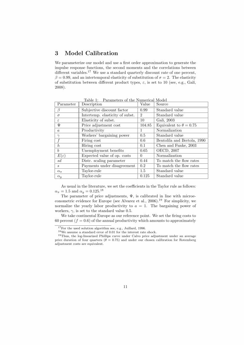
We parameterize our model and use a first order approximation to generate theimpulse response functions, the second moments and the correlations betweendifferent variables.17 We use a standard quarterly discount rate of one percent,β = 0.99, and an intertemporal elasticity of substitution of σ = 2. The elasticityof substitution between different product types, ε, is set to 10 (see, e.g., Galı,2008).

Table 1: Parameters of the Numerical ModelParameter Description Value Source

β Subjective discount factor 0.99 Standard valueσ Intertemp. elasticity of subst. 2 Standard valueε Elasticity of subst. 10 Gali, 2003Ψ Price adjustment cost 104.85 Equivalent to θ = 0.75a Productivity 1 Normalizationγ Workers’ bargaining power 0.5 Standard valuef Firing cost 0.6 Bentolila and Bertola, 1990h Hiring cost 0.1 Chen and Funke, 2003b Unemployment benefits 0.65 OECD, 2007E(ε) Expected value of op. costs 0 Normalizationsd Distr. scaling parameter 0.44 To match the flow ratess Payments under disagreement 0.2 To match the flow ratesαπ Taylor-rule 1.5 Standard valueαy Taylor-rule 0.125 Standard value

As usual in the literature, we set the coefficients in the Taylor rule as follows:απ = 1.5 and αy = 0.125.18

The parameter of price adjustments, Ψ, is calibrated in line with microe-conometric evidence for Europe (see Alvarez et al., 2006).19 For simplicity, wenormalize the yearly labor productivity to a = 1. The bargaining power ofworkers, γ, is set to the standard value 0.5.

We take continental Europe as our reference point. We set the firing costs to60 percent (f = 0.6) of the annual productivity which amounts to approximately

17For the used solution algorithm see, e.g., Juillard, 1996.18We assume a standard error of 0.01 for the interest rate shock.19Thus, the log-linearized Phillips curve under Calvo price adjustment under an average

price duration of four quarters (θ = 0.75) and under our chosen calibration for Rotembergadjustment costs are equivalent.

11

68 percent of the annual wage20 and the hiring costs to 10 percent (h = 0.1)21,22

of annual productivity. In our numerical exercise we will do robustness checkswith respect to the magnitude of labor turnover costs. We set the unemploymentbenefits to 65 percent of the level of productivity (b = 0.65). This implies, thatin steady state the wage replacement rate is roughly 74 percent, which is in linewith evidence for continental European countries (see OECD, 2007).

Operating costs are assumed to follow a logistic distribution with zero mean.23

The scaling parameter of the distribution and the payments under disagreement,s, are chosen in such a way that the resulting labor market flow rates matchthe empirical hiring and firing rates described further below. This yields a scaleparameter of 0.44 and payments under disagreement of 0.2.

We calibrate our flow rates using evidence for West Germany, as there areonly Kaplan-Meier functions for individual countries.24 But we will show fur-ther below that these flow numbers are line with other important continentalEuropean countries. Wilke’s, 2005, Kaplan-Meier functions indicate that about20 percent of the unemployed leave their status after one quarter. For a steadystate unemployment rate of 9 percent, a quarterly separation rate of 2 per-cent is necessary. This is roughly in line with Wilke’s estimated yearly risk ofunemployment. Further, we assume that the steady state share of exogenousseparations is two thirds. This is in line with Krause and Lubik, 2007, andGerman evidence (see, e.g., Erlinghagen, 2005).

The used flow numbers are in line with the OECD, 2004, numbers for othercontinental European countries.25 We conclude that a quarterly job-finding rateof η = 0.20 and a firing rate of φ = 0.02 are reasonable averages for continentalEuropean countries.

20For the period from 1975 to 1986 Bentolila and Bertola, 1990, calculate firing costs of92 percent, 75 percent and 108 percent of the respective annual wage in France, Germanyand Italy respectively. The OECD, 2004, reports that many European countries have reducedtheir job security legislation somewhat from the late 1980 to 2003 (in terms of the overallemployment protection legislation strictness). Therefore, we consider f = 0.6 to be a realisticnumber for continental European countries.

21See Chen and Funke, 2005. Empirical studies on training costs show that training costsare very substantial. Dolfin, 2006, shows that the average training time of a worker takes201 hours (i.e., roughly 25 working days) during the first quarter of employment. Thus,our number is probably rather a lower bound. To the best of our knowledge, there is nocorresponding evidence for Europe.

22The choice of hiring costs vary widely in the search and matching literature. WhileAndolfatto, 1996, Thomas and Zanetti, 2009 or Gertler and Trigari, 2009 use hiring costs ofapproximately 1 percent of output, Shimer, 2005, uses 4 percent, Hall, 2005, uses 8 percentand Mortensen and Pissarides, 1999, use 15 percent. Thus, with our choice we lie well in themiddle of the values used in the literature.

23The logistic distribution is very close to the normal distribution, but has an explicit closedform expressions.

24We choose the Kaplan-Meier functions for Germany, as it is the largest continental Euro-pean country.

25Although the numbers of the OECD outlook are not directly applicable to our model,since they are built on a monthly basis, it is possible to adjust them using a method describedin Shimer, 2007.

12

4 Labor Turnover Costs and Output Persistence

This section demonstrates how labor turnover costs affect the response of out-put to monetary and real shocks. We first consider an uncorrelated iid shockto the central bank’s Taylor rule. We next consider an autocorrelated shockto aggregate productivity. Finally, we illustrate in more detail the role of la-bor turnover costs on output persistence and demonstrate that our model alsogenerates output persistence for lower values of labor turnover costs.

4.1 One-Off Interest Rate Shock

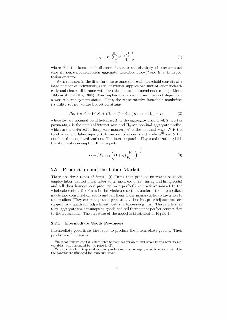
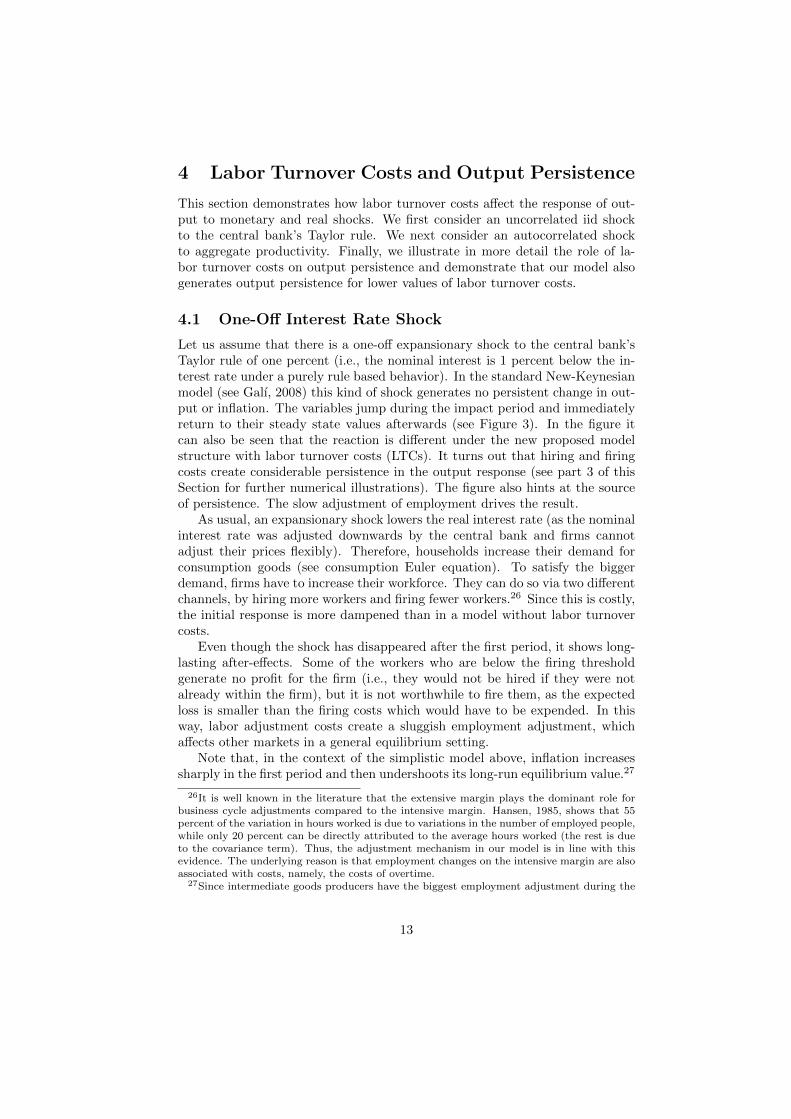
Let us assume that there is a one-off expansionary shock to the central bank’sTaylor rule of one percent (i.e., the nominal interest is 1 percent below the in-terest rate under a purely rule based behavior). In the standard New-Keynesianmodel (see Galı, 2008) this kind of shock generates no persistent change in out-put or inflation. The variables jump during the impact period and immediatelyreturn to their steady state values afterwards (see Figure 3). In the figure itcan also be seen that the reaction is different under the new proposed modelstructure with labor turnover costs (LTCs). It turns out that hiring and firingcosts create considerable persistence in the output response (see part 3 of thisSection for further numerical illustrations). The figure also hints at the sourceof persistence. The slow adjustment of employment drives the result.

As usual, an expansionary shock lowers the real interest rate (as the nominalinterest rate was adjusted downwards by the central bank and firms cannotadjust their prices flexibly). Therefore, households increase their demand forconsumption goods (see consumption Euler equation). To satisfy the biggerdemand, firms have to increase their workforce. They can do so via two differentchannels, by hiring more workers and firing fewer workers.26 Since this is costly,the initial response is more dampened than in a model without labor turnovercosts.

Even though the shock has disappeared after the first period, it shows long-lasting after-effects. Some of the workers who are below the firing thresholdgenerate no profit for the firm (i.e., they would not be hired if they were notalready within the firm), but it is not worthwhile to fire them, as the expectedloss is smaller than the firing costs which would have to be expended. In thisway, labor adjustment costs create a sluggish employment adjustment, whichaffects other markets in a general equilibrium setting.

Note that, in the context of the simplistic model above, inflation increasessharply in the first period and then undershoots its long-run equilibrium value.27

26It is well known in the literature that the extensive margin plays the dominant role forbusiness cycle adjustments compared to the intensive margin. Hansen, 1985, shows that 55percent of the variation in hours worked is due to variations in the number of employed people,while only 20 percent can be directly attributed to the average hours worked (the rest is dueto the covariance term). Thus, the adjustment mechanism in our model is in line with thisevidence. The underlying reason is that employment changes on the intensive margin are alsoassociated with costs, namely, the costs of overtime.

27Since intermediate goods producers have the biggest employment adjustment during the

13

0 2 4 6 8 100

0.1

0.2

0.3

0.4

Quarters

OUTPUT PATH (% DEVIATION)

Model with LTCSStandard Model

0 2 4 6 8 10−0.5

0

0.5

1

1.5

2

2.5

Quarters

INFLATION (ANNUALIZED)

0 2 4 6 8 100

0.1

0.2

0.3

0.4

Quarters

EMPLOYMENT RATE (% DEVIATION)

0 2 4 6 8 100

0.1

0.2

0.3

0.4

Quarters

CONSUMPTION (% DEVIATION)

Figure 3: Reaction to an uncorrelated interest-rate shock in the model withLTCs and in the standard model

This counterfactual result is no longer present when monetary shocks are suffi-ciently autocorrelated, as shown in the working paper version of this paper (seeLechthaler et al., 2008).28

4.2 Productivity Shocks

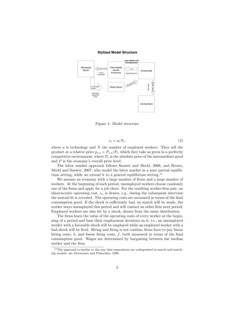
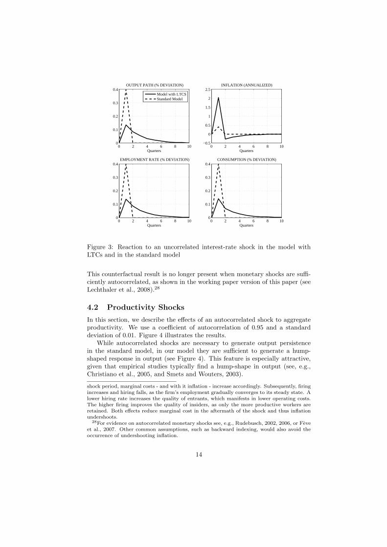
In this section, we describe the effects of an autocorrelated shock to aggregateproductivity. We use a coefficient of autocorrelation of 0.95 and a standarddeviation of 0.01. Figure 4 illustrates the results.

While autocorrelated shocks are necessary to generate output persistencein the standard model, in our model they are sufficient to generate a hump-shaped response in output (see Figure 4). This feature is especially attractive,given that empirical studies typically find a hump-shape in output (see, e.g.,Christiano et al., 2005, and Smets and Wouters, 2003).

shock period, marginal costs - and with it inflation - increase accordingly. Subsequently, firingincreases and hiring falls, as the firm’s employment gradually converges to its steady state. Alower hiring rate increases the quality of entrants, which manifests in lower operating costs.The higher firing improves the quality of insiders, as only the more productive workers areretained. Both effects reduce marginal cost in the aftermath of the shock and thus inflationundershoots.

28For evidence on autocorrelated monetary shocks see, e.g., Rudebusch, 2002, 2006, or Feveet al., 2007. Other common assumptions, such as backward indexing, would also avoid theoccurrence of undershooting inflation.

14

0 10 20 30 400

0.5

1

1.5

Quarters

OUTPUT PATH (% DEVIATION)

Model with LTCSStandard Model

0 10 20 30 40−2

−1.5

−1

−0.5

0

Quarters

INFLATION (ANNUALIZED)

0 10 20 30 40−0.4

−0.2

0

0.2

0.4

0.6

Quarters

EMPLOYMENT RATE (% DEVIATION)

0 10 20 30 400

0.5

1

1.5

Quarters

CONSUMPTION (% DEVIATION)

Figure 4: Reaction to a autocorrelated productivity shock in the model withLTCs and in the standard model

Again this result is due to labor turnover costs. Hiring and firing costs implythat adjusting output is costly. Therefore, the impact reaction is dampened. Bycontrast, in later periods the level of output is already high and therefore furtherincreases are relatively cheap. In other words, due to turnover costs the firmwants to smooth out the adjustment of the workforce.

In contrast, in the standard model without any adjustment costs, the outputjumps up to its highest level in the first period and then slowly converges backto its steady state level, one-to-one with the movement in productivity. Notethat, although the first reaction in output in our model is dampened by laborturnover costs, the jump in output is still larger than in the standard model.This is due to the decrease in employment in the standard model, as can be seenin the lower left panel of Figure 4, which counteracts the increase in output dueto the increase in productivity. In our model, by contrast, employment increases(rather than decreases) in the immediate aftermath of the shock due to the laborturnover costs.29

29It should be kept in mind, that in the standard model employment adjusts via the inten-sive margin, i.e., hours worked, while in our model adjustment takes place via the extensivemargin. The employment reaction to productivity shocks is a hotly debated empirical issue.Some authors find a negative employment reaction after positive productivity shocks (see, forexample, Galı, 1999), while others find the opposite (see, for example, Dedola and Neri, 2007).

15

1 2 3 4 5 6 7 8 9 10

0.02

0.04

0.06

0.08

0.1

0.12

0.14

Quarters

OUTPUT PATH AFTER MONETARY SHOCK (IN % DEVIATION)

fc = 0.5fc = 0.6fc = 0.7

5 10 15 20 25 30 35 40

0.3

0.4

0.5

0.6

0.7

0.8

0.9

1

1.1

1.2

1.3

Quarters

OUTPUT PATH AFTER PRODUCTIVITY SHOCK (IN % DEVIATION)

fc = 0.5fc = 0.6fc = 0.7

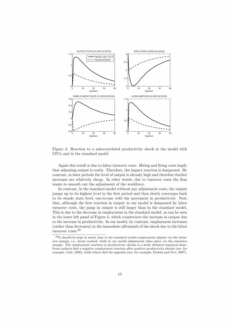
Figure 5: The effect of different firing costs

4.3 The Effect of Labor Turnover Costs

The purpose of this section is twofold. On the one hand, we want to show thatboth hiring and firing costs tend to increase persistence. On the other hand, wewill demonstrate that our model can generate a lot of persistence even for fairlylow labor turnover costs.

In our model, labor turnover costs have two effects. First, they change thesteady states. Lower labor turnover costs lead to higher employment rates andmore production. This corresponds to the observation that the United Stateshave higher employment rates and lower labor turnover costs than Europe.30

Second, as will be shown below, labor turnover costs increase output persistencein response to monetary and real shocks.

To illustrate that, Figure 5 compares our standard calibration with an econ-omy where firing costs are somewhat lower and somewhat higher than in thebaseline calibration (i.e., 50 and 70 percent of the annual wage respectively in-stead of 60 percent as before), keeping all other deep parameters constant. Forcomparability reasons (as there are steady state movements), we express all theeffects in terms of percentage deviations from the respective steady state. Theleft hand panel shows the impulse response function after a one-period interest-rate shock, while the right hand panel illustrates an autocorrelated productivityshock. As before the autoregressive component is set to 0.95.

Figure 5 shows that higher labor turnover costs lead to more output per-sistence. The larger the firing costs are, the more sluggish is the adjustmentprocess after both, interest rate and productivity shocks. While the adjustmentduring the impact period is more pronounced in an economy with lower labor

30Under the given model structure, the employment rate does not generally increase withlower firing costs. For the chosen calibration this is however the case, as the hiring rate reactsmore elastically than the firing rate (due to the calibration of the operating costs). Thisfeature is in line with recent empirical evidence, which shows that hiring is more importantthan firing to explain the business cycle dynamics (see, e.g., Shimer, 2005).

16

1 2 3 4 5 6 7 8 9 10

0.02

0.04

0.06

0.08

0.1

0.12

0.14

Quarters

OUTPUT PATH AFTER MONETARY SHOCK (IN % DEVIATION)

hc = 0.01hc = 0.1hc = 0.2

5 10 15 20 25 30 35 400.2

0.4

0.6

0.8

1

1.2

1.4

Quarters

OUTPUT PATH AFTER PRODUCTIVITY SHOCK (IN % DEVIATION)

hc = 0.01hc = 0.1hc = 0.2

Figure 6: The effect of different hiring costs

adjustment costs, the economy also returns more quickly to the steady state(i.e., shows less persistence). Thus, the adjustment is slowed down by laborturnover costs. Note, however, that even for lower values of firing costs outputis still considerably more persistent than in the standard model.

Figure 6 repeats the same exercise for varying degrees of hiring costs. Similarto firing costs, hiring costs tend to lead to more sluggish responses and higherpersistence. Note, however, that the effects are relatively small and so our modelstill generates a large degree of output persistence even when we lower the hiringcosts to 1%.

Given the fact, that European countries have considerably higher firing costs,our model would thus predict that persistence is higher in Europe than in theUS. The evidence on the volatility of business cycles across countries is mixed.Backus et al., 1995, find that the unconditional volatilities in Europe (for out-put and employment) are lower than in the United States. This is consonantwith the predictions of our model. However, there is also evidence from Vec-torautoregressions (VARs) that shows that the reactions to monetary policyshocks in Europe and in the United States are very similar (see, e.g., Angeloniet al., 2003).

One way to resolve this possible contradiction to our model would be to con-sider realistic countervailing effects (which, for brevity, we have not included inthe model above). For example, it can be shown that the more competitive areproduct markets, the greater is the corresponding degree of output persistencein response to monetary shocks.31 Since product markets in the US generally areconsidered more competitive than those in Europe, on average, this mechanismwould be one way to reconcile our model with the evidence from VARs. Fur-thermore, micro-econometric studies suggest a higher degree of price stickinessin Europe than in the United States (see, for example, Bils and Klenow, 2004,and Alvarez et al., 2006), and this, too, has implications for the comparative

31See, for example, Merkl and Snower, 2009, for more details.

17

degree of monetary persistence.Moreover, it would be premature to believe that the empirical literature has

resolved the question about whether monetary shocks are equally persistent inEurope and the US. In recent studies in this area, the microeconomic structureof estimated medium scale models for Europe and the United States (Smets andWouters, 2003 and 2007) is specified in a similar manner. Thus these studiesexamine the data with the same priors on the labor market structure. This maybe responsible for the fact that these estimated models generate similar amountsof monetary persistence for Europe and the United States. It remains for futureresearch to examine whether the specification of different labor market struc-tures in Europe and the United States - reflecting differences in labor marketinstitutions in these areas - may lead to different results concerning comparativemonetary persistence.

5 Business Cycle Statistics

To be able to make more profound statements on the performance of our model,we compare the second moments of our model to the properties of time seriesdata. As hiring and firing costs are particularly relevant in Europe, we havecalibrated our model economy to a typical continental European country. Un-fortunately, the relevant labor market data for the euro zone is not available.32

Thus, we compare the volatilities generated by the model to data from Ger-many, the largest European economy. The labor market facts are taken fromGartner et al., 2009,33 and the aggregate data on output and inflation from theOECD, 2009.

We proceed in two steps. First, we compare our model to the standard NewKeynesian model (NKM), using productivity and interest rate shocks. Second,we compare our model to Krause and Lubik, 2007, who simulate a NKM witha matching function and endogenous separations. For comparability reasons,we replace our interest rate rule with money demand and money supply distur-bances in this exercise, as in Krause and Lubik, 2007.

In line with the analysis above, we consider productivity shocks and interestrate shocks (i.e., aggregate supply and demand disturbances) when we compareour model to the standard NKM. Both exercises are done for an interest raterule with and without interest rate smoothing34 and compared to the outcome of

32Christoffel et al., 2009, have constructed a labor market data set for the euro zone. Note,however, that it does not contain important variables such as the job-finding rate and theseparation rate.

33For data availability reasons, we have to constrain ourselves to the time period from1977-2004. See Gartner et al., 2009, for details.

34We adjust the Taylor rule,(

1+it1+ı

)=

(1+it−1

1+ı

)αs((πt

π

)απ(

yty

)αy)1−αs

eλt , and set the

smoothing parameter, αs, to 0.8. The autocorrelation of the productivity shock is set to 0.95and the standard errors of the interest rate and productivity shocks are set to 0.15% and0.5% respectively. These numbers are broadly in line with de la Croix et al., 2007, and Smetsand Wouters, 2003, 2005. Note that the productivity shock plays the dominant role in thebusiness cycle statistics with both shocks. However, medium scale model contain several

18

Table

2:Businesscyclestatistics

RelativeSD

Correlations

Auto

correlations

yπ

ujfr

jdr

u,jfr

jfr,jdr

y,π

uy

πData

1.00

0.18

7.34

9.35

2.65

-0.91

-0.53

0.40

0.98

0.92

0.57

Productivityshock,

LTC

1.00

0.37

3.70

4.11

1.71

-0.78

-1.00

-0.98

0.97

0.92

0.96

withoutsm

oothing

NKM

1.00

0.41

--

--

--1.00

-0.88

0.88

Productivityshock,

LTC

1.00

0.44

3.88

3.82

1.59

-0.84

-1.00

-0.83

0.98

0.94

0.59

withsm

oothing

NKM

1.00

0.43

--

--

--0.85

-0.94

0.75

Interest

shock,

LTC

1.00

3.12

10.00

29.34

12.20

-0.65

-1.00

0.66

0.59

0.59

-0.13

withoutsm

oothing

NKM

1.00

0.26

--

--

-1.00

--0.03

-0.03

Interest

shock,

LTC

1.00

2.57

10.00

23.94

9.96

-0.63

-1.00

0.64

0.74

0.74

0.02

withsm

oothing

NKM

1.00

0.59

--

--

-1.00

-0.53

0.53

Jointshocks,

LTC

1.00

0.49

3.96

4.33

1.80

-0.79

-1.00

-0.71

0.97

0.94

0.47

withsm

oothing

NKM

1.00

0.46

--

--

--0.47

-0.88

0.69

Notes:

Data:1977-2004.Relativestandard

dev

iationsdivided

bySD

ofGDP.

LTC:model

withlabortu

rnover

costs.

NKM:standard

New

Key

nesianmodel.

19

the standard NKM. We also consider both shocks simultaneously. As noted, ourmodel generates substantial inflation, output, and unemployment persistencein response to productivity shocks (see last three columns in Table 2). Theautocorrelations for inflation, output and unemployment under productivityshocks with interest rate smoothing are very close to what can be found in theactual data. In a similar vein, our model generates output and unemploymentpersistence in response to interest rate shocks (with and without smoothing).Note, that both our model and the standard NKM do not perform well inreplicating inflation persistence in response to an interest rate shock. Therefore,medium scale NKMs (see, e.g., Smets andWouters, 2003, Christiano et al., 2005)introduce additional adjustment mechanisms to increase inflation persistence.Of course, these mechanisms would also increase inflation persistence in ourmodel.

Our simple labor market model provides a new mechanism to the NKM,which generates considerable persistence and richer dynamics (see, for example,the correlation between output and inflation, which is not -1 or 1 any more).Note that in the standard model, output and inflation persistence in responseto a productivity shock (without interest rate smoothing) basically follow thepersistence of the underlying shock,35 while they are considerably larger in ourmodel.36 With the two joint shocks, we can roughly replicate the autocorrela-tions that can be found in the data.

In the data, the standard deviation of the job-finding rate and the unemploy-ment rate are several times larger than the standard deviation of output. Ourmodel shows a strong amplification mechanism both for productivity shocks andinterest rate shocks. Table 2 also shows that the amplification effect for interestrate shocks is stronger than for productivity shocks.37 This result is in linewith Balleer, 2009, who shows in a VAR estimation that the conditional volatil-ity of job finding and unemployment to technology shocks is smaller than theunconditional volatility, leaving a large role to non-technology disturbances.38

The standard search and matching model does not have a strong amplifica-tion mechanism (see Costain and Reiter, 2008, and Shimer, 2005). This problemhas led to a growing literature trying to solve this puzzle: Hall, 2005, introduces

demand shocks, thereby giving more weight to them. See Table 3 for an example where thedemand shock is more important.

35The autocorrelation of inflation and output is the same as the autocorrelation of theproductivity shock in the standard NKM.

36Den Haan et al., 2000, show that search and matching frictions also increases persistence.However, their model uses physical capital and flexible prices and is, therefore, not directlycomparable to ours.

37Supply shocks change the production possibility frontier (yt = atnt) and generate short-run adjustment dynamics, which both affect the output path. In contrast, demand shocksonly have the latter effect, thereby leading to smaller output variations (for given labor mar-ket variations). This explains why the standard deviations of the job-finding rate and theunemployment rate divided by the standard deviation of output are larger under demandshocks.

38Note that Balleer, 2009, did this analysis for the United States. So far, there is no evidenceon this issue for Europe.

20

wage rigidity, Hagedorn and Manovskii, 2008,39 suggest an alternative calibra-tion, Cooper et al., 2007, build many additional features into the model, suchas fixed and linear costs of vacancy posting, while Den Haan et al., 2000, in-troduce physical capital.40 In contrast, our model offers a completely differentapproach, using a standard calibration, flexible wages41 and a very simple andtractable structure.

The intuition for the amplification effect works as follows: Since the agentsin our model face heterogeneous match-specific shocks, supply or demand shocksaffect the range of match-specific shocks over which firms are willing to makejob offers. Since aggregate productivity shocks are autocorrelated and demandshocks lead to strong and persistent changes in the price for intermediate goods(pz), they have a substantial leverage effect on the expected present value ofprofits generated by newly hired workers, and thereby a strong effect on thehiring thresholds (which directly affects the job-finding rate and thus unem-ployment).

This effect is not at play in the standard search and matching model, asthe creation of new jobs is primarily driven by the matching function and notthe match-specific heterogeneities. This is certainly true with exogenous separa-tions, where heterogeneities plays no role at all. But it is also true for search andmatching models with endogenous separations, as they are typically calibrated.In these models, match-specific heterogeneities are used to calibrate the appro-priate job-destruction rate, which is equal to the probability that a new contactthrough the matching function is destroyed. In our model, all the dynamics aredriven by match-specific heterogeneities. Linear hiring and firing costs drivea wedge between the probability of finding a job, which is reduced by linearhiring costs, and the probability that an existing job continues to exist, whichis raised by linear firing costs. This generates markedly different dynamics thanin a standard search and matching model.

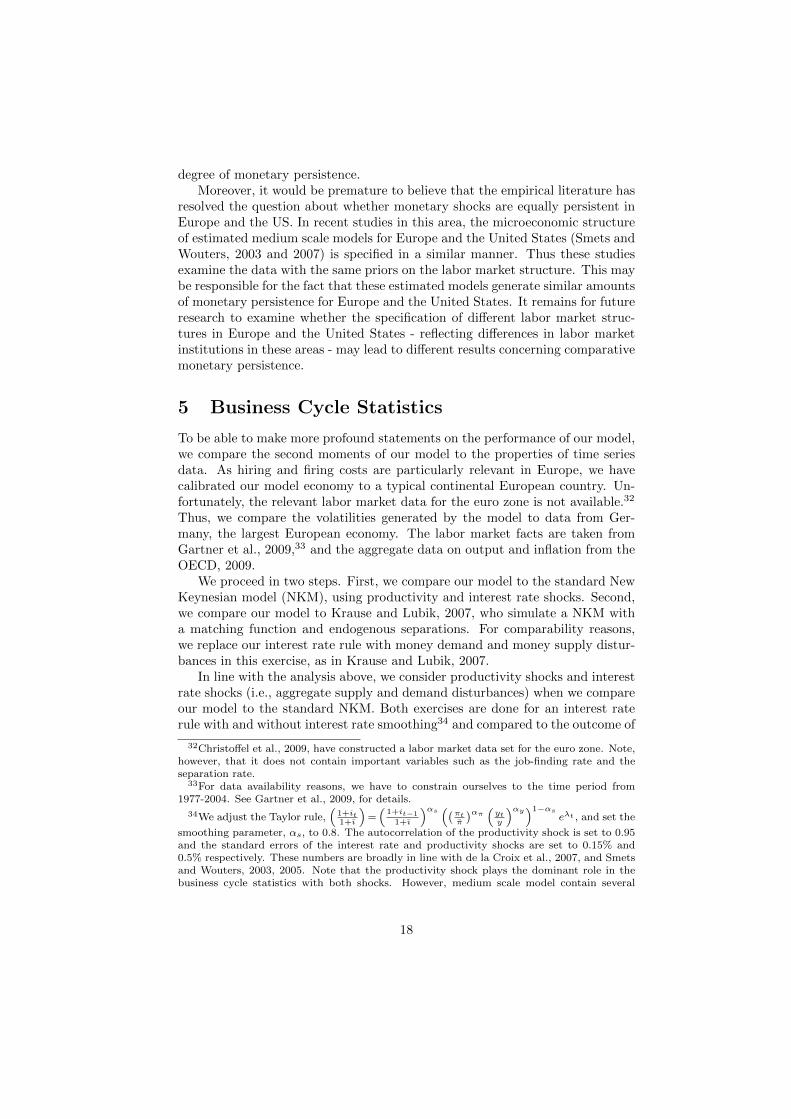
Having shown, that our model can replicate several important stylized facts,we proceed with a careful comparison of our model with models using the match-ing function. The paper that is closest to ours is Krause and Lubik, 2007. Theyuse a New Keynesian model with a matching function and endogenous sepa-rations (and without capital accumulation42). In Table 3,43 we compare theproperties of the two models. For comparability reasons, we also use money

39For a discussion of the disadvantages of these two approaches, see Hornstein et al., 2005.40See Feve and Langot, 1996, for a similar model, estimated for France and Cheron and

Langot, 2000, for a model with sticky prices.41Under our reference calibration, the standard deviation of wages is about 77% of the

standard deviation of productivity. When we change the calibration to make wages andproductivity move one to one, the amplification effect shows only slight changes.

42For real business cycle models with capital accumulation see, for example, Andolfatto,1996, Feve and Langot, 1996, and Den Haan et al., 2000.

43Note that the German data refers to the job-finding rate (i.e., new matches divided byunemployment), while Krause and Lubik (2007) and our business cycle statistics refer to thejob creation rate. The job creation rate is defined as new matches divided by employmentin the previous period. The US data and the KL results are taken from Krause and Lubik(2007).

21

Table 3: Business cycle statistics - comparison with Krause and Lubik, 2007German US LTC KL LTC KL LTC KLdata data PS PS MS MS JS JS

Rel. SDU 7.34 6.90 5.26 4.36 10.00 8.20 5.55 4.98JCR 9.35 2.55 4.68 7.87 23.25 17.17 6.67 9.44JDR 2.65 3.73 2.29 8.00 8.72 22.94 2.89 11.02Corr.JCR, JDR -0.53 -0.36 -0.36 0.28 -0.88 0.18 -0.60 0.34Y, inflation 0.40 0.39 -0.11 -0.11 0.63 0.97 0.01 0.12Autocorr.Output 0.92 0.87 0.96 0.98 0.81 0.78 0.96 0.95Inflation 0.57 0.56 0.25 0.60 0.11 0.60 0.19 0.61

Notes: PS: Productivity shock MS: Shock to money supply, JS: Joint shock.

supply shocks instead of interest rate shocks.44 In contrast to Krause und Lu-bik, 2007,45 our model is able to replicate a negative sign for the correlationbetween the job creation rate and the job destruction rate. In our model, thejob creation and job destruction are both driven by the endogenous cut-offpoints for the idiosyncratic match specific shocks. Thus, when job creation in-creases, job destruction decreases and vice versa. This result holds for bothdemand and supply shocks. Note that the search and matching model withendogenous separations generates counterfactual signs for the correlation be-tween job creation and job destruction. The intuition is straightforward. Theendogenous separation rate reacts very sensitively to aggregate shocks (due toan endogenous movement of the cut-off points), thereby changing the unem-ployment rate very quickly. This affects the ability of the matching function togenerate new contacts. Assume a positive productivity shock, which will reducethe unemployment rate. As a consequence, the matching function’s ability tocreate additional matches is reduced and the job destruction rate and job cre-ation rate move in the same direction (see Figure 3 in Krause and Lubik, 2007).Another striking difference between the two models is that the separation ratein Krause and Lubik, 2007, is too volatile, which is not the case in our model.

In a nutshell, our model can replicate many important features of the data,which other models cannot account for. First, in contrast to the standard NewKeynesian model with frictionless labor markets, it generates output and un-employment persistence. Second, in contrast to the search and matching model

44We use the same numbers as Krause and Lubik, 2007. The standard deviation of theproductivity shock and the money shock are 0.0049 and 0.00623, respectively. The coeffi-cients of autocorrelation for the productivity shock and the money shock are 0.95 and 0.49,respectively. To obtain a money demand function, we add money to our utility function(U(Mt) = log (Mt/Pt)).

45Note that Krause and Lubik, 2007, use a US calibration. However, Merkl and van Roye,2009, show that Krause and Lubik’s model has very similar properties with a Europeancalibration.

22

with exogenous separations, it offers a strong amplification mechanism for thejob-finding rate and the unemployment rate in response to supply and demandshocks. Third, in contrast to the search and matching model with endogenousseparations, it generates realistic correlations between the job creation rate andthe job destruction rate.

6 Conclusion

This paper has offered a new labor market mechanism for the amplification andpropagation of real and monetary shocks. In contrast to the standard small scalemodel, our model generates output and unemployment persistence in responseto uncorrelated monetary shocks (deviations from the central bank’s systematicrule). Further, it generates inflation, output and unemployment persistence inresponse to real shocks. Since hiring and firing costs reduce labor market flows,they make the labor market’s reaction to monetary and macroeconomic shocksmore sluggish. The slow reaction of the labor market is transmitted to theproduct market, thereby generating persistence.

The model offers a strong amplification mechanism in response to macroe-conomic shocks (i.e., the job-finding rate and the unemployment are a lot morevolatile than output). And the model generates a strong negative correlationbetween the job creation rate and the job destruction rate.

23

7 Acknowledgements

We would like to thank Marty Eichenbaum, Ester Faia, Stefan Gerlach, KeithKuester, Camille Logeay, Roland Winkler and the participants of the IfW staffseminar, the Bundesbank-IWH workshop, the LoWER workshop, the EES kick-off workshop, seminars at the Deutsche Bundesbank, Oesterreichische Nation-albank, Free University Berlin, Humboldt University Berlin, the universitiesof Hamburg, Dortmund and Wurzburg, the Annual Meeting of the EuropeanEconomic Association and the German Economic Association for very valuablesuggestions. We thank Dennis Wesselbaum for excellent research assistance. Allremaining errors are our own.

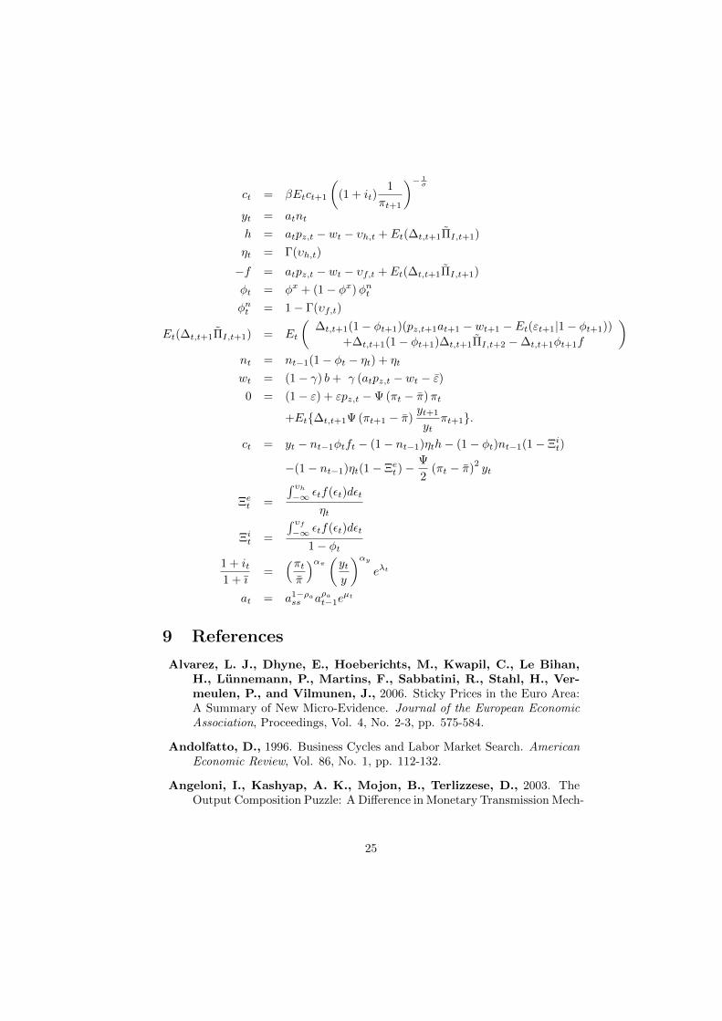
8 Appendix: Set of Nonlinear Equations

To the convenience of the reader, the main equations of the model shall berepeated here. We have 16 endogenous variables: a, c, y, i, vh, η, vf , φ, φ

n, n,

w, pz, π, Ξe, Ξi, ΠI and the 16 equations are:

24

ct = βEtct+1

((1 + it)

1

πt+1

)− 1σ

yt = atnt

h = atpz,t − wt − υh,t + Et(∆t,t+1ΠI,t+1)

ηt = Γ(υh,t)

−f = atpz,t − wt − υf,t + Et(∆t,t+1ΠI,t+1)

φt = φx + (1− φx)φnt

φnt = 1− Γ(υf,t)

Et(∆t,t+1ΠI,t+1) = Et

(∆t,t+1(1− φt+1)(pz,t+1at+1 − wt+1 − Et(εt+1|1− φt+1))

+∆t,t+1(1− φt+1)∆t,t+1ΠI,t+2 −∆t,t+1φt+1f

)

nt = nt−1(1− φt − ηt) + ηt

wt = (1− γ) b+ γ (atpz,t − wt − ε)

0 = (1− ε) + εpz,t −Ψ(πt − π)πt

+Et{∆t,t+1Ψ(πt+1 − π)yt+1

ytπt+1}.

ct = yt − nt−1φtft − (1− nt−1)ηth− (1− φt)nt−1(1− Ξit)

−(1− nt−1)ηt(1− Ξet )−

Ψ

2(πt − π)

2yt

Ξet =

∫ υh

−∞ εtf(εt)dεt

ηt

Ξit =

∫ υf

−∞ εtf(εt)dεt

1− φt

1 + it1 + ı

=(πt

π

)απ(yty

)αy

eλt

at = a1−ρass aρa

t−1eµt

9 References

Alvarez, L. J., Dhyne, E., Hoeberichts, M., Kwapil, C., Le Bihan,H., Lunnemann, P., Martins, F., Sabbatini, R., Stahl, H., Ver-meulen, P., and Vilmunen, J., 2006. Sticky Prices in the Euro Area:A Summary of New Micro-Evidence. Journal of the European EconomicAssociation, Proceedings, Vol. 4, No. 2-3, pp. 575-584.

Andolfatto, D., 1996. Business Cycles and Labor Market Search. AmericanEconomic Review, Vol. 86, No. 1, pp. 112-132.

Angeloni, I., Kashyap, A. K., Mojon, B., Terlizzese, D., 2003. TheOutput Composition Puzzle: A Difference in Monetary Transmission Mech-

25

anism in the Euro Area and the United States. Journal of Money, Credit,and Banking, Vol. 35, No. 6, pp. 1265-1306.

Backus, D., Kehoe, P. and Kydland, F., 1995. International Business Cy-cles: Theory and Evidence. in Cooley, Thomas, ed., Frontiers of BusinessCycles Research, Princeton University Press, Princeton, pp. 331-356.

Balleer, A., 2009. New Evidence, Old Puzzles: Technology Shocks and LaborMarket Dynamics. Kiel Working Paper, No. 1500.

Barnichon, R., 2008. Productivity, Aggregate Demand and UnemploymentFluctuations. Working Paper, No. 47/2008, Federal Reserve Board.

Bentolila, S. and Bertola, G., 1990. Firing Costs and Labour Demand:How Bad is Eurosclerosis. Review of Economic Studies, Vol. 57, pp.381-402.

Bils, M., and Klenow, P., 2004. Some Evidence on the Importance of StickyPrices. Journal of Political Economy, Vol. 112, No. 5, pp. 947-985.

Blanchard, O., and Gali, J., 2010. Labor Markets and Monetary Policy: ANew Keynesian Model with Unemployment. American Economic Journal- Macroeconomics, forthcoming.

Botero, J. C., Djankov, S., Porta, R., and Lopez-De-Silanes, F., 2004.The Regulation of Labor. The Quarterly Journal of Economics, Vol. 119,No. 4, pp. 1339-1382.

Brown, A., Merkl, C., and Snower, D., 2007. Comparing the Effective-ness of Employment Subsidies. IZA Discussion Paper, No. 2835, June2007.

Campbell, J. and Fisher, J., 2000. Aggregate Employment Fluctuationswith Microeconomic Asymmetries. American Economic Review, Vol. 90,No. 5, pp. 1323-1345.

Chen, Y., and Funke, M., 2005. Non-wage Labour Costs, Policy Uncer-tainty and Labour Demand: A Theoretical Assessment. Scottish Journalof Political Economy, Vol. 52, No. 5, pp. 687-709.

Cheron, A., and Langot, F., 2004. Labor Market Search and Real Busi-ness Cycles: Reconciling Nash Bargaining with the Real Wage Dynamics.Review of Economic Dynamics, Vol. 7, No. 2, 476-493.

Cheron, A., and Langot, F., 2000. The Phillips and Beveridge CurvesRevisited. Economics Letters, Vol. 69, pp. 371-376.

Christiano, L. J., Eichenbaum, M., and Evans, C., 2005. NominalRigidities and the Dynamic Effects of a Shock to Monetary Policy. Journalof Political Economy, Vol. 113, No. 1, pp. 1-45.

26

Christoffel, K., and Linzert, T., 2006. The Role of Real Wage Rigidityand Labor Market Frictions for Unemployment and Inflation Dynamics.Bundesbank Discussion Paper, Economic Research Centre: Series 1, No.11/2006, April 2006.

Christoffel, K, Kuester, K., and Linzert, T., 2009. The Role of LaborMarkets for Euro Area Monetary Policy. European Economic Review, Vol.53, pp. 908-936.

Cooper, R., Haltiwanger, J. and Willis, J., 2005. Search Frictions:Matching Aggregate and Establishment Observations. Journal of Mone-tary Economics, Vol. 54, pp. 56-78.

Costain, J., and Reiter, M., 2008. Business Cycles, Unemployment In-surance, and the Calibration of Matching Models. Journal of EconomicDynamics and Control, Vol. 32, No. 4, pp. 1120-1155.

de la Croix, D., de Walque, G., and Wouters, R., 2007. Dynamics andMonetary Policy in a Fair Wage Model of the Business Cycle. EuropeanCentral Bank Working Paper, No. 780.

Dedola, L., and Neri, S., 2007. What Does a Technology Shock Do? AVAR Analysis with Model-Based Sign Restrictions. Journal of MonetaryEconomics, Vol. 54, pp. 512-549.

Den Haan, W., Ramey, G. and Watson, J., 2000. Job Destruction andPropagation of Shocks. American Economic Review, Vol. 90, No. 3, pp.482-498.

Dolfin, S. 2006. An Examination of Firms’ Employment Costs. AppliedEconomics.” Vol. 38, No. 8, pp. 861-878.

Erlinghagen, M., 2005. Lay Offs and Job Security in the Course of Time.Zeitschrift fur Soziologie, Vol. 34, No. 2, pp. 147-168.

Faia, E., 2008. Optimal Monetary Policy Rules with Labor Market Frictions.Journal of Economic Dynamics and Control, Vol. 32, No. 5, pp. 1600-1621.

Feve, P., Matheron, J., and Poilly, C., 2007. Monetary Policy Dynamicsin the Euro Area. Economics Letters, Vol. 96, No. 1, pp. 97-102.

Feve, P., and Langot, F., 1996. Unemployment and the Business Cycle in aSmall Open Economy: G.M.M. estimation and testing with French data.Journal of Economic Dynamics and Control, Vol. 20, pp. 1609-1639.

Galı, J., 1999. Technology, Employment, and the Business Cycle: Do Tech-nology Shocks Explain Aggregate Fluctuations? American EconomicReview, Vol. 89 (1), pp. 249-271.

27

Galı, J., 2008. Monetary Policy, Inflation, and the Business Cycle: An Intro-duction to the New Keynesian Framework. Princeton University Press.

Gartner, H., Merkl, C., and Rothe, T., 2009. They Are Even Larger!More (on) Puzzling Labor Market Volatilities. IAB Discussion Paper, No.12/2009.

Gertler, M., and Trigari, A., 2009. Unemployment Fluctuations withStaggered Nash Wage Bargaining. Journal of Political Economy, Vol.117, No. 1, pp. 38-86.

Hagedorn, M., and Iourii M., 2008. The Cyclical Behavior of EquilibriumUnemployment and Vacancies Revisited. American Economic Review,Vol. 98, No. 4, pp. 1692-1706.

Hall, R., 2005. Employment Fluctuations with Equilibrium Wage Stickiness.American Economic Review, Vol. 95, No. 1, pp. 50-65.

Hall, R. and Milgrom, P., 2008. The Limited Influence of Unemploymenton the Wage Bargain. American Economic Review, Vol. 98, No. 4, pp.1653-1674.

Hansen, G. D., 1985. Indivisible Labor and the Business Cycle. Journal ofMonetary Economics, Vol. 16, pp. 309-327.

Hornstein, A., Krussell, P., and Violante, G. L., 2005. Unemploymentand Vacancy Fluctuations in the Matching Model: Inspecting the Mech-anism. Federal Reserve Bank of Richmond Economic Quarterly, 91(3):19-51.

Juillard, M., 1996. Dynare: A Program for the Resolution and Simulation ofDynamic Models with Forward Variables. CEPREMAP Working Paper,No. 9602.

Krause, M. U., and Lubik, T. A., 2007. The (Ir)relevance of Real WageRigidity in the New Keynesian Model with Search Frictions. Journal ofMonetary Economics, Vol. 54, No. 3, pp. 706-727.

Lechthaler, W., Merkl, C., and Snower, D., 2008. Monetary Persistenceand the Labor Market: A New Perspective. IZA Discussion Paper, No.3513.

Merkl, C., and Snower, D., 2009. Monetary Persistence, Imperfect Com-petition, and Staggering Complementarities. Macroeconomic Dynamics,Vol. 13, No. 1, pp. 81-106.

Merkl, C., and van Roye, B., 2009. European Unemployment Dynamics:Looking into the Black Box. mimeo, Kiel Institute for the World Economy.

Merz, M. 1995. Search in the Labor Market and the Real Business Cycle.Journal of Monetary Economics, Vol. 36, No. 2, pp. 269-300.

28

Mortensen, D., and Pissarides, C., 1999. New developments in models ofsearch in the labor market, in Ashenfelter, Orley and Card, David, eds.,Handbook of Labor Economics, pp. 2567-2627.

OECD, 2004. OECD Employment Outlook 2004. Organization for EconomicCooperation and Development, Paris.

OECD, 2007. Benefits and Wages: OECD Indicators 2007. Organization forEconomic Cooperation and Development, Paris.

OECD, 2009. OECD Statistics. Organization for Economic Cooperation andDevelopment, Paris.

Rotemberg, J., and Woodford, M., 1999. The Cyclical Behavior of Pricesand Costs. Handbook of Macroeconomics, Vol. 1B, pp. 1051-1135.

Rudebusch, G., 2002. Term Structure Evidence on Interest Rate Smoothingand Monetary Policy Inertia. Journal of Monetary Economics, Vol. 49,pp. 1161-1187.

Rudebusch, G., 2006. Monetary Policy Inertia: Fact or Fiction? Interna-tional Journal of Central Banking, Vol. 2, No. 3, pp. 85-135.

Shimer, R., 2005. The Cyclical Behavior of Equilibrium Unemployment andVacancies. American Economic Review, Vol. 95, No. 1, pp. 25-49.

Shimer, R., 2007. Reassessing the Ins and Outs of Unemployment. NBERWorking Paper, No. 13421, September 2007.

Smets, F., and Wouters, R., 2003. An Estimated Dynamic StochasticGeneral Equilibrium Model of the Euro Area. Journal of the EuropeanEconomic Association, Vol. 1, No. 5, pp. 1123-1175.

Smets, F., and Wouters, R., 2005. Comparing Shocks and Frictions in USand Euro Area Business Cycles: A Bayesian DSGE Approach. Journal ofApplied Econometrics, Vol. 20, No. 2, pp. 161-183.

Smets, F., and Wouters, R., 2007. Shock and Frictions in US BusinessCycles: A Bayesian DSGE Approach. American Economic Review, Vol.97, No. 3, pp. 586-606.

Snower, D., and Merkl, C., 2006. The Caring Hand that Cripples: The EastGerman Labor Market after Unification. American Economic Review,Papers and Proceedings, Vol. 96, No. 2, pp. 375-382.

Thomas, C., 2008. Search and Matching Frictions and Optimal MonetaryPolicy. Journal of Monetary Economics, Vol. 55, No. 5, pp. 936-956.

Thomas, C. and Zanetti, F., 2009. Labor Market Reform and Price Stabil-ity: An Application to the Euro Area. Journal of Monetary Economics,Vol. 56, No. 6, pp. 885-899 .

29

Veracierto, M., 2008. Firing Costs and Business Cycle Fluctuations. Inter-national Economic Review, Vol. 49, No. 1, pp. 1-39.

Walsh, C., 2005. Labor Market Search, Sticky Prices, and Interest RatePolicies. Review of Economic Dynamics, Vol. 8, No. 4, 829-849.

Wilke, R., 2005. New Estimates of the Duration and Risk of Unemploymentfor West-Germany. Journal of Applied Social Science Studies, Vol. 125,No. 2, pp. 207-237.

Woodford, M., 2007. Interpreting Inflation Persistence: Comments on theConference on ”Quantitative Evidence on Price Determination”. Journalof Money, Credit and Banking, Supplement to Vol. 39, No. 1, pp. 203-210.

World Bank, 2008. Doing Business 2009. The World Bank Group, Washing-ton.

30

CESifo Working Paper Series for full list see Twww.cesifo-group.org/wp T (address: Poschingerstr. 5, 81679 Munich, Germany, [email protected])

___________________________________________________________________________ 2873 Burkhard Heer and Alfred Maußner, Computation of Business-Cycle Models with the

Generalized Schur Method, December 2009 2874 Carlo Carraro, Enrica De Cian and Massimo Tavoni, Human Capital Formation and

Global Warming Mitigation: Evidence from an Integrated Assessment Model, December 2009

2875 André Grimaud, Gilles Lafforgue and Bertrand Magné, Climate Change Mitigation

Options and Directed Technical Change: A Decentralized Equilibrium Analysis, December 2009

2876 Angel de la Fuente, A Mixed Splicing Procedure for Economic Time Series, December

2009 2877 Martin Schlotter, Guido Schwerdt and Ludger Woessmann, Econometric Methods for

Causal Evaluation of Education Policies and Practices: A Non-Technical Guide, December 2009

2878 Mathias Dolls, Clemens Fuest and Andreas Peichl, Automatic Stabilizers and Economic

Crisis: US vs. Europe, December 2009 2879 Tom Karkinsky and Nadine Riedel, Corporate Taxation and the Choice of Patent

Location within Multinational Firms, December 2009 2880 Kai A. Konrad, Florian Morath and Wieland Müller, Taxation and Market Power,

December 2009 2881 Marko Koethenbuerger and Michael Stimmelmayr, Corporate Taxation and Corporate

Governance, December 2009 2882 Gebhard Kirchgässner, The Lost Popularity Function: Are Unemployment and Inflation

no longer Relevant for the Behaviour of Germany Voters?, December 2009 2883 Marianna Belloc and Ugo Pagano, Politics-Business Interaction Paths, December 2009 2884 Wolfgang Buchholz, Richard Cornes and Dirk Rübbelke, Existence and Warr Neutrality

for Matching Equilibria in a Public Good Economy: An Aggregative Game Approach, December 2009

2885 Charles A.E. Goodhart, Carolina Osorio and Dimitrios P. Tsomocos, Analysis of

Monetary Policy and Financial Stability: A New Paradigm, December 2009 2886 Thomas Aronsson and Erkki Koskela, Outsourcing, Public Input Provision and Policy

Cooperation, December 2009

2887 Andreas Ortmann, “The Way in which an Experiment is Conducted is Unbelievably

Important”: On the Experimentation Practices of Economists and Psychologists, December 2009

2888 Andreas Irmen, Population Aging and the Direction of Technical Change, December

2009 2889 Wolf-Heimo Grieben and Fuat Şener, Labor Unions, Globalization, and Mercantilism,

December 2009 2890 Conny Wunsch, Optimal Use of Labor Market Policies: The Role of Job Search

Assistance, December 2009 2891 Claudia Buch, Cathérine Tahmee Koch and Michael Kötter, Margins of International

Banking: Is there a Productivity Pecking Order in Banking, too?, December 2009 2892 Shafik Hebous and Alfons J. Weichenrieder, Debt Financing and Sharp Currency

Depreciations: Wholly vs. Partially Owned Multinational Affiliates, December 2009 2893 Johannes Binswanger and Daniel Schunk, What is an Adequate Standard of Living

during Retirement?, December 2009 2894 Armin Falk and James J. Heckman, Lab Experiments are a Major Source of Knowledge

in the Social Sciences, December 2009 2895 Hartmut Egger and Daniel Etzel, The Impact of Trade on Employment, Welfare, and

Income Distribution in Unionized General Oligopolistic Equilibrium, December 2009 2896 Julian Rauchdobler, Rupert Sausgruber and Jean-Robert Tyran, Voting on Thresholds

for Public Goods: Experimental Evidence, December 2009 2897 Michael McBride and Stergios Skaperdas, Conflict, Settlement, and the Shadow of the

Future, December 2009 2898 Ben J. Heijdra and Laurie S. M. Reijnders, Economic Growth and Longevity Risk with

Adverse Selection, December 2009 2899 Johannes Becker, Taxation of Foreign Profits with Heterogeneous Multinational Firms,

December 2009 2900 Douglas Gale and Piero Gottardi, Illiquidity and Under-Valuation of Firms, December

2009 2901 Donatella Gatti, Christophe Rault and Anne-Gaël Vaubourg, Unemployment and

Finance: How do Financial and Labour Market Factors Interact?, December 2009 2902 Arno Riedl, Behavioral and Experimental Economics Can Inform Public Policy: Some

Thoughts, December 2009

2903 Wilhelm K. Kohler and Marcel Smolka, Global Sourcing Decisions and Firm

Productivity: Evidence from Spain, December 2009 2904 Marcel Gérard and Fernando M. M. Ruiz, Corporate Taxation and the Impact of

Governance, Political and Economic Factors, December 2009 2905 Mikael Priks, The Effect of Surveillance Cameras on Crime: Evidence from the

Stockholm Subway, December 2009 2906 Xavier Vives, Asset Auctions, Information, and Liquidity, January 2010 2907 Edwin van der Werf, Unilateral Climate Policy, Asymmetric Backstop Adoption, and

Carbon Leakage in a Two-Region Hotelling Model, January 2010 2908 Margarita Katsimi and Vassilis Sarantides, Do Elections Affect the Composition of

Fiscal Policy?, January 2010 2909 Rolf Golombek, Mads Greaker and Michael Hoel, Climate Policy without Commitment,

January 2010 2910 Sascha O. Becker and Ludger Woessmann, The Effect of Protestantism on Education

before the Industrialization: Evidence from 1816 Prussia, January 2010 2911 Michael Berlemann, Marco Oestmann and Marcel Thum, Demographic Change and

Bank Profitability. Empirical Evidence from German Savings Banks, January 2010 2912 Øystein Foros, Hans Jarle Kind and Greg Shaffer, Mergers and Partial Ownership,

January 2010 2913 Sean Holly, M. Hashem Pesaran and Takashi Yamagata, Spatial and Temporal

Diffusion of House Prices in the UK, January 2010 2914 Christian Keuschnigg and Evelyn Ribi, Profit Taxation and Finance Constraints,

January 2010 2915 Hendrik Vrijburg and Ruud A. de Mooij, Enhanced Cooperation in an Asymmetric

Model of Tax Competition, January 2010 2916 Volker Meier and Martin Werding, Ageing and the Welfare State: Securing

Sustainability, January 2010 2917 Thushyanthan Baskaran and Zohal Hessami, Globalization, Redistribution, and the

Composition of Public Education Expenditures, January 2010 2918 Angel de la Fuente, Testing, not Modelling, the Impact of Cohesion Support: A

Theoretical Framework and some Preliminary Results for the Spanish Regions, January 2010

2919 Bruno S. Frey and Paolo Pamini, World Heritage: Where Are We? An Empirical

Analysis, January 2010

2920 Susanne Ek and Bertil Holmlund, Family Job Search, Wage Bargaining, and Optimal

Unemployment Insurance, January 2010 2921 Mariagiovanna Baccara, Allan Collard-Wexler, Leonardo Felli and Leeat Yariv, Gender

and Racial Biases: Evidence from Child Adoption, January 2010 2922 Kurt R. Brekke, Roberto Cellini, Luigi Siciliani and Odd Rune Straume, Competition

and Quality in Regulated Markets with Sluggish Demand, January 2010 2923 Stefan Bauernschuster, Oliver Falck and Niels Große, Can Competition Spoil

Reciprocity? – A Laboratory Experiment, January 2010 2924 Jerome L. Stein, A Critique of the Literature on the US Financial Debt Crisis, January

2010 2925 Erkki Koskela and Jan König, Profit Sharing, Wage Formation and Flexible

Outsourcing under Labor Market Imperfection, January 2010 2926 Gabriella Legrenzi and Costas Milas, Spend-and-Tax Adjustments and the

Sustainability of the Government’s Intertemporal Budget Constraint, January 2010 2927 Piero Gottardi, Jean Marc Tallon and Paolo Ghirardato, Flexible Contracts, January

2010 2928 Gebhard Kirchgässner and Jürgen Wolters, The Role of Monetary Aggregates in the

Policy Analysis of the Swiss National Bank, January 2010 2929 J. Trent Alexander, Michael Davern and Betsey Stevenson, Inaccurate Age and Sex

Data in the Census PUMS Files: Evidence and Implications, January 2010 2930 Stefan Krasa and Mattias K. Polborn, Competition between Specialized Candidates,

January 2010 2931 Yin-Wong Cheung and Xingwang Qian, Capital Flight: China’s Experience, January

2010 2932 Thomas Hemmelgarn and Gaetan Nicodeme, The 2008 Financial Crisis and Taxation

Policy, January 2010 2933 Marco Faravelli, Oliver Kirchkamp and Helmut Rainer, Social Welfare versus

Inequality Concerns in an Incomplete Contract Experiment, January 2010 2934 Mohamed El Hedi Arouri and Christophe Rault, Oil Prices and Stock Markets: What

Drives what in the Gulf Corporation Council Countries?, January 2010 2935 Wolfgang Lechthaler, Christian Merkl and Dennis J. Snower, Monetary Persistence and

the Labor Market: A New Perspective, January 2010