arXiv:1903.00966v3 [cond-mat.stat-mech] 19 Jan 2020 1 Moment theories for a d-dimensional dilute granular gas of Maxwell molecules Vinay Kumar Gupta 1,2, † 1 Discipline of Mathematics, Indian Institute of Technology Indore, Indore 453552, India 2 Mathematics Institute, University of Warwick, Coventry CV4 7AL, UK (Received xx; revised xx; accepted xx) Various systems of moment equations—consisting of up to (d + 3)(d 2 +6d + 2)/6 moments—in a general dimension d for a dilute granular gas composed of Maxwell molecules are derived from the inelastic Boltzmann equation by employing the Grad moment method. The Navier–Stokes-level constitutive relations for the stress and heat flux appearing in the system of mass, momentum and energy balance equations are determined from the derived moment equations. It has been shown that the moment equations only for the hydrodynamic field variables (density, velocity and granular temperature), stress and heat flux—along with the time-independent value of the fourth cumulant—are sufficient for determining the Navier–Stokes-level constitutive relations in the case of inelastic Maxwell molecules, and that the other higher-order moment equations do not play any role in this case. The homogeneous cooling state of a freely cooling granular gas is investigated with the system of the Grad (d + 3)(d 2 +6d + 2)/6- moment equations and its various subsystems. By performing a linear stability analysis in the vicinity of the homogeneous cooling state, the critical system size for the onset of instability is estimated through the considered Grad moment systems. The results on critical system size from the presented moment theories are found to be in reasonably good agreement with those from simulations. 1. Introduction Under strong excitation, granular materials resemble ordinary (molecular) gases and are referred to as rapid granular flows or granular gases (Campbell 1990; Goldhirsch 2003). The prototype model of a granular gas is a dilute system comprised of smooth (frictionless) identical hard spheres—with no interstitial fluid—colliding pairwise and inelastically with a constant coefficient of (normal) restitution 0 e 1, with e =0 referring to perfectly sticky collisions and e = 1 to perfectly elastic collisions (Campbell 1990; Goldhirsch 2003; Brilliantov & P¨ oschel 2004; Garz´ o 2019). In the dilute limit, this system can be described by a single-particle velocity distribution function, which is the fundamental quantity in kinetic theory and obeys the Boltzmann equation suitably modified to incorporate energy dissipation due to inelastic collisions. The resemblance of granular gases to ordinary gases has motivated the development of several kinetic theory based tools for granular gases by suitably modifying these tools to account for energy dissipation due to inelastic collisions in the last three decades, and it is still an active area of research; see, e.g., Jenkins & Richman (1985a ,b ); Sela & Goldhirsch (1998); Brey et al. (1998a ); Garz´ o & Santos (2003); Santos (2003); Brilliantov & P¨ oschel (2004); Bisi et al. (2004); Garz´ o & Santos (2011); Kremer & Marques Jr. (2011); Garz´ o (2013); Khalil et al. (2014); Kremer et al. (2014); Gupta & Shukla (2017); Gupta et al. (2018); † Email address for correspondence: [email protected]

Welcome message from author
This document is posted to help you gain knowledge. Please leave a comment to let me know what you think about it! Share it to your friends and learn new things together.
Transcript
arX
iv:1
903.
0096
6v3
[co
nd-m
at.s
tat-
mec
h] 1
9 Ja
n 20
201
Moment theories for a d-dimensional dilutegranular gas of Maxwell molecules
Vinay Kumar Gupta1,2,†1Discipline of Mathematics, Indian Institute of Technology Indore, Indore 453552, India
2Mathematics Institute, University of Warwick, Coventry CV4 7AL, UK
(Received xx; revised xx; accepted xx)
Various systems of moment equations—consisting of up to (d + 3)(d2 + 6d + 2)/6moments—in a general dimension d for a dilute granular gas composed of Maxwellmolecules are derived from the inelastic Boltzmann equation by employing the Gradmoment method. The Navier–Stokes-level constitutive relations for the stress and heatflux appearing in the system of mass, momentum and energy balance equations aredetermined from the derived moment equations. It has been shown that the momentequations only for the hydrodynamic field variables (density, velocity and granulartemperature), stress and heat flux—along with the time-independent value of the fourthcumulant—are sufficient for determining the Navier–Stokes-level constitutive relationsin the case of inelastic Maxwell molecules, and that the other higher-order momentequations do not play any role in this case. The homogeneous cooling state of a freelycooling granular gas is investigated with the system of the Grad (d+ 3)(d2 + 6d+ 2)/6-moment equations and its various subsystems. By performing a linear stability analysisin the vicinity of the homogeneous cooling state, the critical system size for the onsetof instability is estimated through the considered Grad moment systems. The results oncritical system size from the presented moment theories are found to be in reasonablygood agreement with those from simulations.
1. Introduction
Under strong excitation, granular materials resemble ordinary (molecular) gases andare referred to as rapid granular flows or granular gases (Campbell 1990; Goldhirsch2003). The prototype model of a granular gas is a dilute system comprised of smooth(frictionless) identical hard spheres—with no interstitial fluid—colliding pairwise andinelastically with a constant coefficient of (normal) restitution 0 6 e 6 1, with e = 0referring to perfectly sticky collisions and e = 1 to perfectly elastic collisions (Campbell1990; Goldhirsch 2003; Brilliantov & Poschel 2004; Garzo 2019). In the dilute limit,this system can be described by a single-particle velocity distribution function, which isthe fundamental quantity in kinetic theory and obeys the Boltzmann equation suitablymodified to incorporate energy dissipation due to inelastic collisions. The resemblanceof granular gases to ordinary gases has motivated the development of several kinetictheory based tools for granular gases by suitably modifying these tools to account forenergy dissipation due to inelastic collisions in the last three decades, and it is still anactive area of research; see, e.g., Jenkins & Richman (1985a,b); Sela & Goldhirsch (1998);Brey et al. (1998a); Garzo & Santos (2003); Santos (2003); Brilliantov & Poschel (2004);Bisi et al. (2004); Garzo & Santos (2011); Kremer & Marques Jr. (2011); Garzo (2013);Khalil et al. (2014); Kremer et al. (2014); Gupta & Shukla (2017); Gupta et al. (2018);
† Email address for correspondence: [email protected]
2 Vinay Kumar Gupta
Garzo (2019). Nevertheless, the non-conservation of energy in granular systems makeskinetic theory based tools much more involved and has profound consequences on theirbehaviour, leading to a raft of intriguing phenomena pertaining to granular matter.Kinetic theory of classical (monatomic) gases offers systematic ways of deriving the
transport equations for the field variables. The two notable approaches in kinetic theory,around which various solution techniques and some other models have been developed,are the Chapman–Enskog (CE) expansion (Chapman & Cowling 1970) and the Gradmoment method (Grad 1949). While these approaches have been instrumental in un-derstanding several problems from a theoretical point of view, both have their ownshortcomings. The former, which is adequate for flows close to equilibrium, considersthe transport equations only for the hydrodynamic field variables (density, velocity andtemperature) and provides the constitutive relations for additional unknowns, namelythe stress and heat flux, in these equations. Despite being successful in deriving theEuler equations (at zeroth order of expansion) and the classical Navier–Stokes andFourier (NSF) equations (at first order of expansion), the usefulness of models (theBurnett equations and beyond) resulting from the higher-order CE expansion remainsscarce mainly due to inherent instabilities (Bobylev 1982). On the other hand, theGrad moment method (Grad 1949) furnishes the governing equations—referred to as themoment equations—for more field variables than the hydrodynamic ones and employs aHermite polynomial expansion to close the system of moment equations. A set of momentequations emanating from the Grad moment method is always linearly stable but suffersfrom the loss of hyperbolicity (Muller & Ruggeri 1998; Cai et al. 2014b)—an essentialproperty for the well-posedness of a system of partial differential equations (PDEs). Theloss of hyperbolicity renders a Grad moment system to show some unphysical behaviour,e.g. unphysical sub-shocks within the shock profile above a critical Mach number. Yet,the Grad moment method has a clear advantage of linearly stable equations and, hence,is preferred over the CE expansion for describing nonequilibrium flows of monatomicgases.To circumvent the problems associated with the Grad moment method, a number of
moment methods have been proposed in the literature. Levermore (1996) propoundedthe maximum-entropy approach for closing a moment system. Although the maximum-entropy approach of Levermore (1996) produces hyperbolic systems of moment equationsby construction, it is extremely difficult to obtain Levermore’s moment equations in anexplicit form beyond the 10-moment case (which does not include the heat flux) becausethe fluxes associated with higher moments cannot be expressed in a closed form. AsLevermore’s 10-moment system is not capable of describing heat conduction, it is not veryuseful for describing gaseous processes. In addition, larger moment systems resulting fromthe maximum-entropy approach are prone to serious mathematical issues (Junk 1998;Junk & Unterreiter 2002). To alleviate problems associated with the maximum-entropyapproach, McDonald & Torrilhon (2013) proposed affordable numerical approximationsto the maximum-entropy closures for problems involving heat transfer and presenteda robust and affordable version of Levermore’s 14-moment system (that includes theheat flux). Although the 14-moment system proposed by McDonald & Torrilhon (2013)is capable of predicting accurate and smooth shock structures even for relatively largeMach numbers, it is not globally hyperbolic. In a completely different approach thatfocused on producing hyperbolic moment equations, Torrilhon (2010) introduced a novelclosure computed with multi-variate Pearson-IV-distributions for the 13-moment system;however the approach seems unlikely to work for higher-order moment systems. Inanother approach, Struchtrup & Torrilhon (2003) introduced a model, termed as theregularised 13-moment (R13) equations, which regularises the original Grad 13-moment
Moment theories for a granular gas of Maxwell molecules 3
(G13) equations by employing a CE-like expansion around a pseudo-equilibrium state.Subsequently, the R13 equations were also derived in an elegant and clean way byStruchtrup (2005) via the order of magnitude approach. The R13 equations are linearlystable, predict smooth shock structure for all Mach numbers and can capture severalrarefaction effects, such as Knudsen layers, with good accuracy for sufficiently smallKnudsen numbers (Struchtrup & Torrilhon 2003; Torrilhon & Struchtrup 2004). To covermore transition-flow regime, Gu & Emerson (2009) employed the regularisation approachof Struchtrup & Torrilhon (2003) to derive the regularised 26-moment (R26) equations.It may be noted, however, that the R13 and R26 equations are also not hyperbolic. TheGrad and regularised moment equations consisting of an arbitrary number of momentshave also been implemented and solved numerically by Cai & Li (2010). In the lastfew years, various other regularisation techniques that yield globally hyperbolic momentequations have been introduced. Cai et al. (2013) proposed a regularisation of the Gradmoment equations in one space dimension based on investigating the properties of theJacobian matrix of fluxes in the system and derived globally hyperbolic moment equations(HME) in one space dimension. Further, Cai et al. (2014a) generalised the method toderive HME in multi-dimension. Koellermeier et al. (2014) employed quadrature-basedprojection methods, which alter the structure of a moment system in a desired way, toobtain hyperbolic systems of the so-called quadrature-based moment equations (QBME).Fan et al. (2016) proposed a generalised framework, which is capable of deriving variousexisting as well as some new systems of regularised hyperbolic moment equations, basedon the so-called operator projection method. A remarkable drawback of HME and QBMEis that they cannot be written in a conservative form (Koellermeier & Torrilhon 2017).Consequently, the standard finite volume schemes cannot be applied to solve systems ofHME and QBME numerically. Recently, some non-conservative numerical schemes havebeen proposed by Koellermeier & Torrilhon (2017, 2018) for the numerical solution ofQBME in one and two dimensions. While numerical methods for solving general three-dimensional unsteady flow problems with moment equations are still intractable, themethod of fundamental solution (MFS) enables us to develop efficient meshfree numericalmethods for solving three-dimensional steady flow problems with the linearised momentequations. Recently, the MFS has been developed for the G13 and R13 equations inLockerby & Collyer (2016) and Claydon et al. (2017), respectively.The system of the R13 equations (also the system of the R26 equations), despite being
non-hyperbolic, may be regarded as the most promising continuum model for describ-ing rarefied monatomic gas flows since it is accompanied with appropriate boundaryconditions (Gu & Emerson 2007; Torrilhon & Struchtrup 2008), and has already beensuccessful in describing a number of canonical flows (see Torrilhon 2016, and referencestherein). Motivated from the accomplishments of the moment method (in particular,the R13 equations) in the case of monatomic gases, the Grad and regularised momentequations have also been developed for monatomic gas mixtures (Gupta & Torrilhon2015; Gupta 2015; Gupta et al. 2016). It is important to note here that the derivationof the regularised moment equations requires higher-order Grad moment equations, forinstance, the derivations of the R13 and R26 equations require the Grad 26-moment(G26) and Grad 45-moment equations, respectively, and that most of the aforementionedworks on the moment method employ either some simplified kinetic models to replacethe Boltzmann collision operator or the Maxwell potential for molecular interactions.The latter, introduced by Maxwell (1867), is inversely proportional to the fourth powerof the distance between the colliding molecules and makes the collision rate independentof the relative velocity between the colliding molecules, which greatly simplifies theoriginal Boltzmann equation. Remarkably, for Maxwell molecules (i.e. for molecules
4 Vinay Kumar Gupta
interacting with the Maxwell interaction potential), the collisional production terms—theterms emanating from the Boltzmann collision operator in the moment equations—canbe computed without the knowledge of explicit form of the distribution function and,moreover, they turn out to be bilinear combinations of moments of the same or lowerorder, resulting into a one-way coupling on the right-hand sides of a moment system.This makes the moment equations for Maxwell molecules tractable. For more details onthe moment method for Maxwell molecules, the reader is referred to a review paper bySantos (2009).The development of kinetic theory of granular gases started out with two semi-
nal works by Jenkins & Savage (1983) and Lun et al. (1984), which introduced kinetictheory for smooth inelastic hard spheres (IHS), followed by the pioneering work ofJenkins & Richman (1985b) on kinetic theory for rough inelastic hard disks (IHD). Theaforementioned methods, namely the CE expansion and the Grad moment method, inkinetic theory of classical gases have also been extended to granular gases, with the maingoal of determining the NSF-level transport coefficients appearing in the expressions forthe stress and heat flux, since the hydrodynamic equations closed with the NSF-levelconstitutive relations are sufficient to describe flows involving small spatial gradients.The CE expansion to zeroth order was first employed by Goldshtein & Shapiro (1995)to obtain the Euler-like hydrodynamic equations for rough granular flows. Subsequently,Brey et al. (1998a) and Garzo & Dufty (1999) determined the NSF-level transport co-efficients for dilute and dense granular gases of IHS, respectively, by means of the first-order CE expansion in powers of a uniformity parameter that estimates the strengthof spatial gradients of the hydrodynamic field variables. The derivation of Burnettequations (i.e. the second-order CE expansion) even for the prototype model of a granulargas is an arduous task. Yet, by performing a generalised CE expansion in powersof two small parameters, namely the Knudsen number and the degree of inelasticity,Sela & Goldhirsch (1998) determined the constitutive relations for the stress and heatflux up to Burnett order for a smooth granular gas of IHS. The requirement of thedegree of inelasticity being small for performing asymptotic expansion limits the validityof Burnett equations derived by Sela & Goldhirsch (1998) to nearly elastic granulargases. Lutsko (2005) further extended the CE expansion to dense granular fluids witharbitrary energy loss models and determined the NSF-level constitutive relations. Notonly did his work consider arbitrary inelasticity but also a velocity-dependent coefficientof restitution, providing the NSF-level constitutive relations for more realistic granularfluids.Granular flows of interest often fall beyond the regime covered by Newtonian hy-
drodynamics since the strength of spatial gradients in flows of practical interest isnot small due to the inherent coupling between the spatial gradients and inelasticity(Goldhirsch 2003). Consequently, for such flows, the granular NSF equations obtainedfrom the first-order CE expansion are not adequate and the Burnett equations for IHSare not meaningful due to their validity being restricted to nearly elastic granular gasesbesides Bobylev’s instability. Such granular flows can alternatively be modelled by theGrad moment method. The method was extended to granular fluids first by Jenkins& Richman who derived the G13 equations for a dense and smooth granular gas ofIHS (Jenkins & Richman 1985a) and the Grad 16-moment equations for a dense andrough granular gas of IHD (Jenkins & Richman 1985b). It is well-established that thefourth cumulant (scalar fourth moment of the velocity distribution function) ought tobe included in the list of the field variables for appropriate description of processes ingranular gases; for instance, a theoretical description of the recently observed Mpembaeffect in granular fluids requires the fourth cumulant as a field variable (Lasanta et al.
Moment theories for a granular gas of Maxwell molecules 5
2017). Keeping that in mind, Risso & Cordero (2002) included the fourth cumulant inthe list of the field variables to derive the Grad 9-moment equations for a bidimensionalgranular gas, and utilised them to investigate the homogeneous cooling state (HCS) andthe steadily heated state of a bidimensional granular gas. Bisi et al. (2004) attempted toextend the Grad moment method to one-dimensional dilute granular flows of viscoelastichard spheres. It may be noted that all the aforementioned works on moment method forgranular fluids are also restricted to nearly elastic particles. The Grad 14-moment (G14)equations for a dilute granular gas of IHS were introduced by Kremer & Marques Jr.(2011) wherein the authors exploited the G14 equations to obtain the NSF-level con-stitutive relations for the stress and heat flux via the Maxwell iteration procedure andto investigate the linear stability of the HCS. Although the G14 equations introducedby Kremer & Marques Jr. (2011) were not restricted to nearly elastic particles, theirprocedure to obtain the constitutive relations did not incorporate the effect of thecollisional dissipation. Consequently, the constitutive relations determined by them arevalid only for nearly elastic granular gases. The issue was resolved by Garzo (2013) whoproposed a procedure to determine the NSF-level constitutive relations incorporatingthe contributions through the collisional dissipation as well. Although the work of Garzo(2013) yielded the accurate NSF-level constitutive relations for moderately dense granulargases in a general dimension, it only computed the collisional contributions to stress andheat flux exploiting the G14 distribution function but did not provide the G14 equationsexplicitly. Very recently, Gupta et al. (2018) derived the fully nonlinear G26 equations fordilute granular gases of IHS. Following the approach of Garzo (2013), they determined theNSF-level constitutive relations for the stress and heat flux through the G26 equations.The coefficient of the shear viscosity found by them through the G26 equations turnedout to be the best among those obtained via any other theory so far. Notwithstanding, theother transport coefficients related to the heat flux obtained through the G26 equationsin Gupta et al. (2018) were exactly the same as those obtained via the CE expansion atthe first Sonine approximation (Brey et al. 1998a) or via the G14 distribution function(Garzo 2013), and the authors adduced that the Grad 29-moment (G29) theory, whichincludes the flux of the fourth cumulant as field variable, would be able to improve thetransport coefficients related to the heat flux.Despite these ever-improving developments, the fact is that the Boltzmann equation
for IHS, and hence the models stemming from the Boltzmann equation for IHS, remainsdifficult to deal with. To circumvent the difficulties pertaining to models for IHS, a modelof inelastic Maxwell molecules (IMM) was proposed at the beginning of this century(Ben-Naim & Krapivsky 2000; Carrillo et al. 2000; Ernst & Brito 2002). Similarly to themodel of Maxwell molecules for monatomic gases, the IMMmodel also makes the collisionrate of the inelastic Boltzmann equation independent of the relative velocity of thecolliding molecules and thereby simplifies the inelastic Boltzmann equation greatly. In thepast few years, the IMM model has received tremendous attention as the simple structureof the Boltzmann collision operator for IMM enables us to describe many propertiesof granular gases analytically, such as the high-velocity tails (Ben-Naim & Krapivsky2002; Ernst & Brito 2002) and the fourth cumulant (Ernst & Brito 2002; Santos 2003)in the HCS, and the NSF-level transport coefficients (Santos 2003). Moreover, theexperimental results on the velocity distribution in driven granular gases composed ofmagnetic grains are well-described by the IMM model (Kohlstedt et al. 2005). The paperby Garzo & Santos (2011) presents a comprehensive review of the IMM model. The tworelevant works here are by Santos (2003) and Khalil et al. (2014), which respectivelyderive the NSF- and Burnett-level transport coefficients for a d-dimensional dilutegranular gas of IMM by means of the CE expansion. It is worthwhile to note that the
6 Vinay Kumar Gupta
work of Khalil et al. (2014), in contrast to that of Sela & Goldhirsch (1998), containsonly one smallness parameter, proportional to the spatial gradient of a hydrodynamicfield, for performing the CE expansion but is not restricted to nearly elastic granulargases. Nevertheless, as also pointed out in Khalil et al. (2014) as a cautionary note,a regularisation of Burnett equations for IMM is apparently necessary to extricateBobylev’s instability. Furthermore, as mentioned above, for a proper description of manyprocesses in granular fluids, it is imperative to include the scalar fourth moment as a fieldvariable. Therefore, a moment-based modelling of granular gases seems to be necessaryfor proper description of processes involving large spatial gradients.
Aiming to the long-term perspective of establishing a complete set of predictivemoment equations—for which appropriate boundary conditions, the MFS for steadyflow problems and a general numerical framework for unsteady flow problems can bedeveloped—for granular gases, the main objective of this paper is to derive the Gradmoment equations—comprising of up to (d + 3)(d2 + 6d + 2)/6 moments—for a d-dimensional dilute (unforced) granular gas of IMM. Here, d = 2 refers to planar diskflows and d = 3 to three-dimensional sphere flows. Following the procedure due toGarzo (2013), the NSF-level transport coefficients for a dilute granular gas of IMM aredetermined from the derived Grad moment equations for IMM. The Grad (d+3)(d2+6d+2)/6-moment equations are then utilised to study the HCS of a freely cooling granulargas of IMM. As it is well-known that the HCS of a granular gas is unstable but theinstabilities are confined to large systems (see, e.g., Brilliantov & Poschel 2004, andreferences therein), the linear stability of the HCS is investigated with the consideredGrad moment systems and the results are employed to estimate the critical system sizefor the onset of instability.
It is worthwhile to note that a Grad moment system for a dilute granular gas differsfrom that for a rarefied monatomic gas only on the right-hand sides by virtue of differentBoltzmann collision operators, therefore it is expected that a Grad moment system fordilute granular gases, similarly to a Grad moment system for monatomic gases, willalso suffer from the loss of hyperbolicity. A detailed investigation of the hyperbolicity ofthe Grad moment systems derived in this paper and their regularisations will, however,be considered elsewhere in the future. From an application point of view, the Gradmoment equations derived in the present work have limited applications at present dueto unavailability of the associated boundary conditions, which are beyond the scope of thepresent paper and will also be considered elsewhere in the future. Nonetheless, the Gradmoment equations developed in this paper can be utilised to investigate problems that donot require boundary conditions, e.g. the shock-tube problem, by employing numericaltechniques specialised to moment equations developed, for example, in Torrilhon (2006);Cai & Li (2010); Koellermeier & Torrilhon (2017).
The layout of the paper is as follows. The Boltzmann equation for IMM and the basictransport equations (i.e. mass, momentum and energy balance equations) for granulargases of IMM are presented in § 2. The considered Grad moment systems are presented in§ 3. The NSF transport coefficients for a dilute granular gas of IMM are determined fromthe Grad moment equations in § 4. The HCS of a freely cooling granular gas is exploredthrough the Grad moment equations in § 5. The linear stability analysis of the HCS isperformed in § 6. The paper ends with a short summary and conclusion in § 7.
Moment theories for a granular gas of Maxwell molecules 7
2. The Boltzmann equation and the hydrodynamic equations for
IMM
We consider a dilute granular gas composed of smooth-identical-inelastic d-dimensionalspherical particles of mass m and diameter d. The state of such a gas can be fullydescribed by a single-particle velocity distribution function f ≡ f(t,x, c)—where t, xand c denote the time, position and instantaneous velocity of a particle, respectively—that obeys the inelastic Boltzmann equation (Brilliantov & Poschel 2004)
∂f
∂t+ ci
∂f
∂xi+ Fi
∂f
∂ci= J [c|f, f ], (2.1)
where F is the external force per unit mass that does not usually depend on c,J [c|f, f ] is the (inelastic) Boltzmann collision operator and the Einstein summationapplies over repeated indices throughout the paper (unless mentioned otherwise). Ford-dimensional IMM, the Boltzmann collision operator has a simplified form given by(Ben-Naim & Krapivsky 2002; Ernst & Brito 2002; Garzo & Santos 2007; Garzo 2019)
J [c|f, f ] = ν
nΩd
∫
Rd
∫
Sd−1
[
1
ef(t,x, c′′) f(t,x, c′′1)− f(t,x, c) f(t,x, c1)
]
dk dc1. (2.2)
In the Boltzmann collision operator for IMM (2.2), e is the (constant) coefficient ofrestitution and ν ≡ ν(e)—a free parameter in the model—is an effective collisionfrequency that is typically chosen in such a way that the results from the Boltzmannequations for IHS and IMM agree in an optimal way (Garzo & Santos 2007). In particular,the agreement of cooling rates from the Boltzmann equations for IHS and IMM leads to(Garzo & Santos 2007; Khalil et al. 2014)
ν =d+ 2
2ν, where ν =
4Ωd√π(d+ 2)
ndd−1
√
T
m(2.3a,b)
is the collision frequency associated with the Navier–Stokes shear viscosity of an elastic(monatomic) gas with Ωd = 2πd/2/Γ (d/2) being the total solid angle in d dimensions,n ≡ n(t,x) the number density and T ≡ T (t,x) the granular temperature, which isa measure of the fluctuating kinetic energy. The velocities c′′ and c′′1 in (2.2) are thepre-collisional velocities of the colliding molecules that transform to the post-collisionalvelocities c and c1 in an inverse collision following the relations (Sela & Goldhirsch 1998;Brilliantov & Poschel 2004):
c′′ = c − 1 + e
2e(k · g)k and c′′1 = c1 +
1 + e
2e(k · g)k, (2.4)
where g = c − c1 is the relative velocity of the colliding molecules, k is the unit vectorjoining the centres of the colliding molecules at the time of collision. The integrationlimits of k in (2.2) extend over the d-dimensional unit sphere Sd−1. Although the limitsof integration will be dropped henceforth for the sake of succinctness, an integration overany velocity space will stand for the volume integral over Rd and that over k will standfor the volume integral over the d-dimensional unit sphere Sd−1.
The hydrodynamic variables—number density n ≡ n(t,x), macroscopic velocity v ≡v(t,x) and granular temperature T ≡ T (t,x)—relate to the velocity distribution functionvia
n(t,x) =
∫
f(t,x, c) dc, (2.5)
8 Vinay Kumar Gupta
n(t,x)v(t,x) =
∫
c f(t,x, c) dc, (2.6)
d
2n(t,x)T (t,x) =
1
2m
∫
C2 f(t,x, c) dc, (2.7)
where C(t,x, c) = c − v(t,x) is the peculiar velocity. The governing equations for thehydrodynamic variables—namely, the mass, momentum and energy balance equations—can be derived from the Boltzmann equation (2.1) by multiplying it with 1, ci and
1dmC2,
and integrating each of the resulting equations over the velocity space successively. Themass, momentum and energy balance equations, respectively, read
Dn
Dt+ n
∂vi∂xi
= 0, (2.8)
DviDt
+1
mn
[
∂σij∂xj
+∂(nT )
∂xi
]
− Fi = 0, (2.9)
DT
Dt+
2
d
1
n
(
∂qi∂xi
+ σij∂vi∂xj
+ nT∂vi∂xi
)
= −ζ T, (2.10)
where D/Dt ≡ ∂/∂t + vk ∂/∂xk is the material derivative. The right-hand sides of themass and momentum balance equations (2.8) and (2.9) vanish due to the conservation ofmass and momentum. However, owing to dissipative collisions among grains, the energyis not conserved, yielding a nonzero right-hand side in the energy balance equation (2.10)with the nonzero cooling rate ζ being given by
ζ = − m
dnT
∫
C2 J [c|f, f ] dc. (2.11)
Furthermore, σij ≡ σij(t,x) and qi ≡ qi(t,x) in (2.9) and (2.10) are the stress tensorand heat flux, respectively, and are given by
σij = m
∫
C〈iCj〉f dc and qi =1
2m
∫
C2Cif dc, (2.12)
where the angle brackets around the indices denote the symmetric and traceless part ofthe corresponding tensor; see appendix A for its definition.
Needless to say, the system of mass, momentum and energy balance equations (2.8)–(2.10) for the hydrodynamic variables n, vi and T is not closed since it encompasses theadditional unknowns σij , qi and ζ, and in order to deal with this system any further,it is indispensable to close it. Typically, the closure for system (2.8)–(2.10) is obtainedby means of the CE expansion, which yields the constitutive relations for σij , qi and ζto various orders of approximation (see, e.g., Brey et al. 1998a; Sela & Goldhirsch 1998;Garzo & Dufty 1999; Gupta 2011; Khalil et al. 2014). However, as also stated in § 1,system (2.8)–(2.10) closed with the constitutive relations obtained at the zeroth and firstorders of the CE expansion is not adequate for describing processes involving large spatialgradients while system (2.8)–(2.10) closed with the constitutive relations obtained at thesecond and higher orders of the CE expansion suffers from Bobylev’s instability. Onthe other hand, the Grad moment method is capable of yielding more accurate modelsthat do not suffer from Bobylev’s instability and are expected to be valid for processesinvolving large spatial gradients. Therefore, in what follows, the Grad moment methodwill be employed for deriving a few closed sets of macroscopic transport equations for ad-dimensional dilute granular gas of IMM.
Moment theories for a granular gas of Maxwell molecules 9
3. Grad moment method
The central goal of the moment method is to have reduced complexity while allowingfor more accurate models for rarefied gases. It is well-known that the direct solutions ofthe Boltzmann equation are computationally expensive since the Boltzmann equation issolved for the velocity distribution function, which depends on total 2d+ 1 variables (1for time, d for space and d for velocity). The idea of moment method is to consider afinite number of equations for moments, instead of the Boltzmann equation, that dependonly on d + 1 variables (1 for time and d for space); and the hope is that a sufficientnumber of moment equations would recover the solution from the Boltzmann equation(to a certain extent). The details of the Grad moment method are skipped here for thesake of brevity but they—for monatomic gases—can be found in Grad (1949) and instandard textbooks, e.g. Struchtrup (2005); Kremer (2010), and—for granular gases ofthree-dimensional hard spheres—in Gupta et al. (2018).Inclusion of the governing equations for the stress (σij) and heat flux (qi) along with the
system of mass, momentum and energy balance equations (2.8)–(2.10) leads to the well-known system of the 13-moment equations in three dimensions. In this paper, some Gradmoment systems consisting of higher-order moments will also be derived and investigated.To this end, it is convenient to introduce a general symmetric-traceless moment
uai1i2...ir := m
∫
C2aC〈i1Ci2 . . . Cir〉 f dc, a, r ∈ N0 (3.1)
and its associated collisional production term (or collisional moment)
Pai1i2...ir := m
∫
C2aC〈i1Ci2 . . . Cir〉 J [c|f, f ] dc, (3.2)
where the angle brackets around the indices again denote the symmetric and traceless partof the corresponding quantity; see appendix A for its definition. From definitions (3.1)and (3.2), it is straightforward to verify that u0 = mn = ρ, u0i = 0, u1 = dnT = d ρ θ,u0ij = σij , u
1i = 2 qi, P0 = P0
i = 0 and P1 = −dnT ζ. Here ρ = mn is the mass densityand θ = T/m.
3.1. Counting moments in d dimensions
Before deriving the various moment systems, it is worthwhile to know how manymoments a Grad moment system contains in a general dimension d. As it is moreconvenient to work with symmetric-traceless moments, the number of moments in aGrad moment system in a general dimension can be determined by knowing the numberof independent components in a symmetric r-rank tensor and the number of traces inthis tensor. Indeed, the number of independent components of a fully symmetric r-rank
tensor in d dimensions is(
d+r−1r
)
= (d+r−1)!r! (d−1)! , and the number of traces in this tensor is
0 for r ∈ 0, 1 while(
d+r−3r−2
)
= (d+r−3)!(r−2)! (d−1)! for r ∈ N \ 1. Consequently, the number
of independent components of a fully symmetric-traceless r-rank tensor (r ∈ N \ 1) ind dimensions is
(
d+ r − 1
r
)
−(
d+ r − 3
r − 2
)
=d+ 2r − 2
d+ r − 2
(
d+ r − 2
r
)
.
Notably, any symmetric-traceless r-rank tensor (r ∈ N) in two dimensions has only twoindependent components while any symmetric-traceless r-rank tensor (r ∈ N) in threedimensions has 2r + 1 independent components. The counting of number of momentsin some of the Grad moment systems considered in this paper is illustrated in table 1.
10 Vinay Kumar Gupta
Field variables Unknowns in d dimensionsUnknowns in3 dimensions
Unknowns in2 dimensions
ρ 1
d2+5d+22!
(d+1)(d2+8d+6)3!
1
13
26
1
8
13
vi d 3 2
θ 1 1 1
σij(d+2)(d−1)
2!5 2
qi d 3 2
u0ijk
(d+4)d(d−1)3!
7 2
u2 1 1 1
u1ij
(d+2)(d−1)2!
5 2
u2i d 3 2
Total (d+3)(d2+6d+2)3!
29 15
Table 1. Number of unknown field variables in Grad moment systems in d dimensions
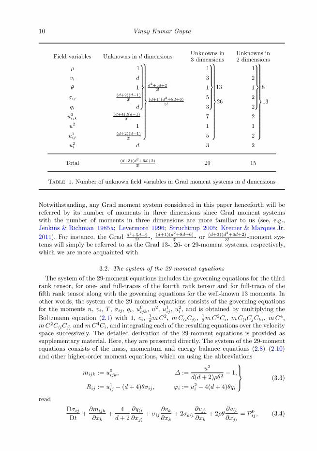
Notwithstanding, any Grad moment system considered in this paper henceforth will bereferred by its number of moments in three dimensions since Grad moment systemswith the number of moments in three dimensions are more familiar to us (see, e.g.,Jenkins & Richman 1985a; Levermore 1996; Struchtrup 2005; Kremer & Marques Jr.
2011). For instance, the Grad d2+5d+22! -, (d+1)(d2+8d+6)
3! - or (d+3)(d2+6d+2)3! -moment sys-
tems will simply be referred to as the Grad 13-, 26- or 29-moment systems, respectively,which we are more acquainted with.
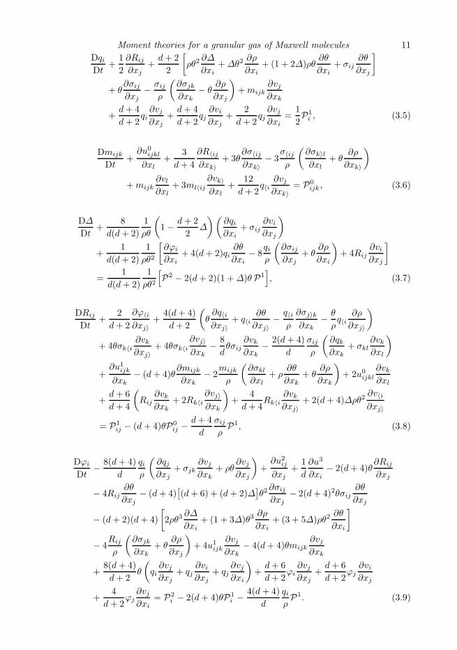
3.2. The system of the 29-moment equations
The system of the 29-moment equations includes the governing equations for the thirdrank tensor, for one- and full-traces of the fourth rank tensor and for full-trace of thefifth rank tensor along with the governing equations for the well-known 13 moments. Inother words, the system of the 29-moment equations consists of the governing equationsfor the moments n, vi, T , σij , qi, u
0ijk, u
2, u1ij , u2i , and is obtained by multiplying the
Boltzmann equation (2.1) with 1, ci,1dmC2, mC〈iCj〉,
12mC2Ci, mC〈iCjCk〉, mC4,
mC2C〈iCj〉 andmC4Ci, and integrating each of the resulting equations over the velocityspace successively. The detailed derivation of the 29-moment equations is provided assupplementary material. Here, they are presented directly. The system of the 29-momentequations consists of the mass, momentum and energy balance equations (2.8)–(2.10)and other higher-order moment equations, which on using the abbreviations
mijk := u0ijk, ∆ :=u2
d(d+ 2)ρθ2− 1,
Rij := u1ij − (d+ 4)θσij , ϕi := u2i − 4(d+ 4)θqi
(3.3)
read
DσijDt
+∂mijk
∂xk+
4
d+ 2
∂q〈i
∂xj〉+ σij
∂vk∂xk
+ 2σk〈i∂vj〉
∂xk+ 2ρθ
∂v〈i
∂xj〉= P0
ij , (3.4)
Moment theories for a granular gas of Maxwell molecules 11
DqiDt
+1
2
∂Rij
∂xj+d+ 2
2
[
ρθ2∂∆
∂xi+∆θ2
∂ρ
∂xi+ (1 + 2∆)ρθ
∂θ
∂xi+ σij
∂θ
∂xj
]
+ θ∂σij∂xj
− σijρ
(
∂σjk∂xk
− θ∂ρ
∂xj
)
+mijk∂vj∂xk
+d+ 4
d+ 2qi∂vj∂xj
+d+ 4
d+ 2qj∂vi∂xj
+2
d+ 2qj∂vj∂xi
=1
2P1i , (3.5)
Dmijk
Dt+∂u0ijkl∂xl
+3
d+ 4
∂R〈ij
∂xk〉+ 3θ
∂σ〈ij∂xk〉
− 3σ〈ijρ
(
∂σk〉l∂xl
+ θ∂ρ
∂xk〉
)
+mijk∂vl∂xl
+ 3ml〈ij
∂vk〉
∂xl+
12
d+ 2q〈i
∂vj∂xk〉
= P0ijk, (3.6)
D∆
Dt+
8
d(d+ 2)
1
ρθ
(
1− d+ 2
2∆
)(
∂qi∂xi
+ σij∂vi∂xj
)
+1
d(d+ 2)
1
ρθ2
[
∂ϕi
∂xi+ 4(d+ 2)qi
∂θ
∂xi− 8
qiρ
(
∂σij∂xj
+ θ∂ρ
∂xi
)
+ 4Rij∂vi∂xj
]
=1
d(d+ 2)
1
ρθ2
[
P2 − 2(d+ 2)(1 +∆)θP1]
, (3.7)
DRij
Dt+
2
d+ 2
∂ϕ〈i
∂xj〉+
4(d+ 4)
d+ 2
(
θ∂q〈i
∂xj〉+ q〈i
∂θ
∂xj〉− q〈i
ρ
∂σj〉k
∂xk− θ
ρq〈i
∂ρ
∂xj〉
)
+ 4θσk〈i∂vk∂xj〉
+ 4θσk〈i∂vj〉
∂xk− 8
dθσij
∂vk∂xk
− 2(d+ 4)
d
σijρ
(
∂qk∂xk
+ σkl∂vk∂xl
)
+∂u1ijk∂xk
− (d+ 4)θ∂mijk
∂xk− 2
mijk
ρ
(
∂σkl∂xl
+ ρ∂θ
∂xk+ θ
∂ρ
∂xk
)
+ 2u0ijkl∂vk∂xl
+d+ 6
d+ 4
(
Rij∂vk∂xk
+ 2Rk〈i
∂vj〉
∂xk
)
+4
d+ 4Rk〈i
∂vk∂xj〉
+ 2(d+ 4)∆ρθ2∂v〈i
∂xj〉
= P1ij − (d+ 4)θP0
ij −d+ 4
d
σijρ
P1, (3.8)
Dϕi
Dt− 8(d+ 4)
d
qiρ
(
∂qj∂xj
+ σjk∂vj∂xk
+ ρθ∂vj∂xj
)
+∂u2ij∂xj
+1
d
∂u3
∂xi− 2(d+ 4)θ
∂Rij
∂xj
− 4Rij∂θ
∂xj− (d+ 4)
[
(d+ 6) + (d+ 2)∆]
θ2∂σij∂xj
− 2(d+ 4)2θσij∂θ
∂xj
− (d+ 2)(d+ 4)
[
2ρθ3∂∆
∂xi+ (1 + 3∆)θ3
∂ρ
∂xi+ (3 + 5∆)ρθ2
∂θ
∂xi
]
− 4Rij
ρ
(
∂σjk∂xk
+ θ∂ρ
∂xj
)
+ 4u1ijk∂vj∂xk
− 4(d+ 4)θmijk∂vj∂xk
+8(d+ 4)
d+ 2θ
(
qi∂vj∂xj
+ qj∂vi∂xj
+ qj∂vj∂xi
)
+d+ 6
d+ 2ϕi∂vj∂xj
+d+ 6
d+ 2ϕj∂vi∂xj
+4
d+ 2ϕj∂vj∂xi
= P2i − 2(d+ 4)θP1
i − 4(d+ 4)
d
qiρP1. (3.9)
12 Vinay Kumar Gupta
The abbreviations (3.3) are introduced in such a way that mijk, ∆, Rij and ϕi vanish ifcomputed with the well-known G13 distribution function
f|G13 = fM
[
1 +1
2
σijCiCj
ρθ2+qiCi
ρθ2
(
1
d+ 2
C2
θ− 1
)]
, (3.10)
where
fM ≡ fM (t,x, c) = n
(
1
2 π θ
)d/2
exp
(
−C2
2 θ
)
(3.11)
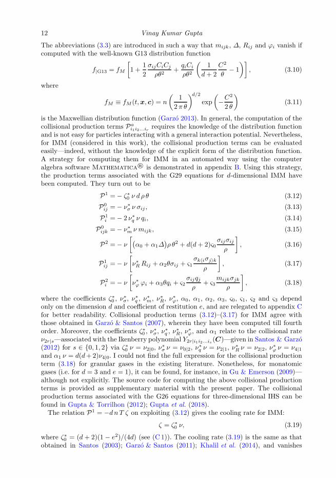
is the Maxwellian distribution function (Garzo 2013). In general, the computation of thecollisional production terms Pa
i1i2...ir requires the knowledge of the distribution functionand is not easy for particles interacting with a general interaction potential. Nevertheless,for IMM (considered in this work), the collisional production terms can be evaluatedeasily—indeed, without the knowledge of the explicit form of the distribution function.A strategy for computing them for IMM in an automated way using the computeralgebra software Mathematica® is demonstrated in appendix B. Using this strategy,the production terms associated with the G29 equations for d-dimensional IMM havebeen computed. They turn out to be
P1 = − ζ∗0 ν d ρ θ (3.12)
P0ij = − ν∗σ ν σij , (3.13)
P1i = − 2 ν∗q ν qi, (3.14)
P0ijk = − ν∗m ν mijk, (3.15)
P2 = − ν
[
(
α0 + α1∆)
ρ θ2 + d(d+ 2)ς0σijσijρ
]
, (3.16)
P1ij = − ν
[
ν∗R Rij + α2θσij + ς1σk〈iσj〉k
ρ
]
, (3.17)
P2i = − ν
[
ν∗ϕ ϕi + α3θqi + ς2σijqjρ
+ ς3mijkσjk
ρ
]
, (3.18)
where the coefficients ζ∗0 , ν∗σ, ν
∗q , ν
∗m, ν∗R, ν
∗ϕ, α0, α1, α2, α3, ς0, ς1, ς2 and ς3 depend
only on the dimension d and coefficient of restitution e, and are relegated to appendix Cfor better readability. Collisional production terms (3.12)–(3.17) for IMM agree withthose obtained in Garzo & Santos (2007), wherein they have been computed till fourthorder. Moreover, the coefficients ζ∗0 , ν
∗σ, ν
∗q , ν
∗R, ν
∗ϕ, and α1 relate to the collisional rate
ν2r|s—associated with the Ikenberry polynomial Y2r|i1i2...is(C)—given in Santos & Garzo(2012) for s ∈ 0, 1, 2 via ζ∗0 ν = ν2|0, ν
∗σ ν = ν0|2, ν
∗q ν = ν2|1, ν
∗R ν = ν2|2, ν
∗ϕ ν = ν4|1
and α1 ν = d(d+2)ν4|0. I could not find the full expression for the collisional productionterm (3.18) for granular gases in the existing literature. Nonetheless, for monatomicgases (i.e. for d = 3 and e = 1), it can be found, for instance, in Gu & Emerson (2009)—although not explicitly. The source code for computing the above collisional productionterms is provided as supplementary material with the present paper. The collisionalproduction terms associated with the G26 equations for three-dimensional IHS can befound in Gupta & Torrilhon (2012); Gupta et al. (2018).The relation P1 = −dnT ζ on exploiting (3.12) gives the cooling rate for IMM:
ζ = ζ∗0 ν, (3.19)
where ζ∗0 = (d + 2)(1 − e2)/(4d) (see (C 1)). The cooling rate (3.19) is the same as thatobtained in Santos (2003); Garzo & Santos (2011); Khalil et al. (2014), and vanishes
Moment theories for a granular gas of Maxwell molecules 13
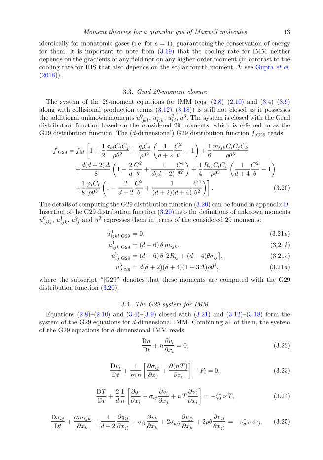
identically for monatomic gases (i.e. for e = 1), guaranteeing the conservation of energyfor them. It is important to note from (3.19) that the cooling rate for IMM neitherdepends on the gradients of any field nor on any higher-order moment (in contrast to thecooling rate for IHS that also depends on the scalar fourth moment ∆; see Gupta et al.(2018)).
3.3. Grad 29-moment closure
The system of the 29-moment equations for IMM (eqs. (2.8)–(2.10) and (3.4)–(3.9)along with collisional production terms (3.12)–(3.18)) is still not closed as it possessesthe additional unknown moments u0ijkl, u
1ijk, u
2ij , u
3. The system is closed with the Graddistribution function based on the considered 29 moments, which is referred to as theG29 distribution function. The (d-dimensional) G29 distribution function f|G29 reads
f|G29 = fM
[
1 +1
2
σijCiCj
ρθ2+qiCi
ρθ2
(
1
d+ 2
C2
θ− 1
)
+1
6
mijkCiCjCk
ρθ3
+d(d+ 2)∆
8
(
1− 2
d
C2
θ+
1
d(d+ 2)
C4
θ2
)
+1
4
RijCiCj
ρθ3
(
1
d+ 4
C2
θ− 1
)
+1
8
ϕiCi
ρθ3
(
1− 2
d+ 2
C2
θ+
1
(d+ 2)(d+ 4)
C4
θ2
)]
. (3.20)
The details of computing the G29 distribution function (3.20) can be found in appendix D.Insertion of the G29 distribution function (3.20) into the definitions of unknown momentsu0ijkl, u
1ijk, u
2ij and u3 expresses them in terms of the considered 29 moments:
u0ijkl|G29 = 0, (3.21a)
u1ijk|G29 = (d+ 6) θmijk, (3.21b)
u2ij|G29 = (d+ 6) θ[
2Rij + (d+ 4)θσij]
, (3.21c)
u3|G29 = d(d+ 2)(d+ 4)(1 + 3∆)ρθ3, (3.21d)
where the subscript “|G29” denotes that these moments are computed with the G29distribution function (3.20).
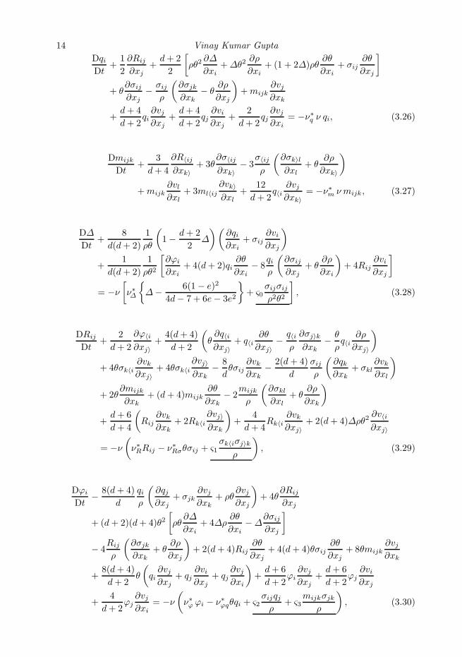
3.4. The G29 system for IMM
Equations (2.8)–(2.10) and (3.4)–(3.9) closed with (3.21) and (3.12)–(3.18) form thesystem of the G29 equations for d-dimensional IMM. Combining all of them, the systemof the G29 equations for d-dimensional IMM reads
Dn
Dt+ n
∂vi∂xi
= 0, (3.22)
DviDt
+1
mn
[
∂σij∂xj
+∂(nT )
∂xi
]
− Fi = 0, (3.23)
DT
Dt+
2
d
1
n
[
∂qi∂xi
+ σij∂vi∂xj
+ nT∂vi∂xi
]
= −ζ∗0 ν T, (3.24)
DσijDt
+∂mijk
∂xk+
4
d+ 2
∂q〈i
∂xj〉+ σij
∂vk∂xk
+ 2σk〈i∂vj〉
∂xk+ 2ρθ
∂v〈i
∂xj〉= −ν∗σ ν σij , (3.25)
14 Vinay Kumar Gupta
DqiDt
+1
2
∂Rij
∂xj+d+ 2
2
[
ρθ2∂∆
∂xi+∆θ2
∂ρ
∂xi+ (1 + 2∆)ρθ
∂θ
∂xi+ σij
∂θ
∂xj
]
+ θ∂σij∂xj
− σijρ
(
∂σjk∂xk
− θ∂ρ
∂xj
)
+mijk∂vj∂xk
+d+ 4
d+ 2qi∂vj∂xj
+d+ 4
d+ 2qj∂vi∂xj
+2
d+ 2qj∂vj∂xi
= −ν∗q ν qi, (3.26)
Dmijk
Dt+
3
d+ 4
∂R〈ij
∂xk〉+ 3θ
∂σ〈ij
∂xk〉− 3
σ〈ij
ρ
(
∂σk〉l
∂xl+ θ
∂ρ
∂xk〉
)
+mijk∂vl∂xl
+ 3ml〈ij
∂vk〉
∂xl+
12
d+ 2q〈i
∂vj∂xk〉
= −ν∗m ν mijk, (3.27)
D∆
Dt+
8
d(d+ 2)
1
ρθ
(
1− d+ 2
2∆
)(
∂qi∂xi
+ σij∂vi∂xj
)
+1
d(d+ 2)
1
ρθ2
[
∂ϕi
∂xi+ 4(d+ 2)qi
∂θ
∂xi− 8
qiρ
(
∂σij∂xj
+ θ∂ρ
∂xi
)
+ 4Rij∂vi∂xj
]
= −ν[
ν∗∆
∆− 6(1− e)2
4d− 7 + 6e− 3e2
+ ς0σijσijρ2θ2
]
, (3.28)
DRij
Dt+
2
d+ 2
∂ϕ〈i
∂xj〉+
4(d+ 4)
d+ 2
(
θ∂q〈i
∂xj〉+ q〈i
∂θ
∂xj〉− q〈i
ρ
∂σj〉k
∂xk− θ
ρq〈i
∂ρ
∂xj〉
)
+ 4θσk〈i∂vk∂xj〉
+ 4θσk〈i∂vj〉
∂xk− 8
dθσij
∂vk∂xk
− 2(d+ 4)
d
σijρ
(
∂qk∂xk
+ σkl∂vk∂xl
)
+ 2θ∂mijk
∂xk+ (d+ 4)mijk
∂θ
∂xk− 2
mijk
ρ
(
∂σkl∂xl
+ θ∂ρ
∂xk
)
+d+ 6
d+ 4
(
Rij∂vk∂xk
+ 2Rk〈i
∂vj〉
∂xk
)
+4
d+ 4Rk〈i
∂vk∂xj〉
+ 2(d+ 4)∆ρθ2∂v〈i
∂xj〉
= −ν(
ν∗RRij − ν∗Rσθσij + ς1σk〈iσj〉k
ρ
)
, (3.29)
Dϕi
Dt− 8(d+ 4)
d
qiρ
(
∂qj∂xj
+ σjk∂vj∂xk
+ ρθ∂vj∂xj
)
+ 4θ∂Rij
∂xj
+ (d+ 2)(d+ 4)θ2[
ρθ∂∆
∂xi+ 4∆ρ
∂θ
∂xi−∆
∂σij∂xj
]
− 4Rij
ρ
(
∂σjk∂xk
+ θ∂ρ
∂xj
)
+ 2(d+ 4)Rij∂θ
∂xj+ 4(d+ 4)θσij
∂θ
∂xj+ 8θmijk
∂vj∂xk
+8(d+ 4)
d+ 2θ
(
qi∂vj∂xj
+ qj∂vi∂xj
+ qj∂vj∂xi
)
+d+ 6
d+ 2ϕi∂vj∂xj
+d+ 6
d+ 2ϕj∂vi∂xj
+4
d+ 2ϕj∂vj∂xi
= −ν(
ν∗ϕ ϕi − ν∗ϕqθqi + ς2σijqjρ
+ ς3mijkσjk
ρ
)
, (3.30)
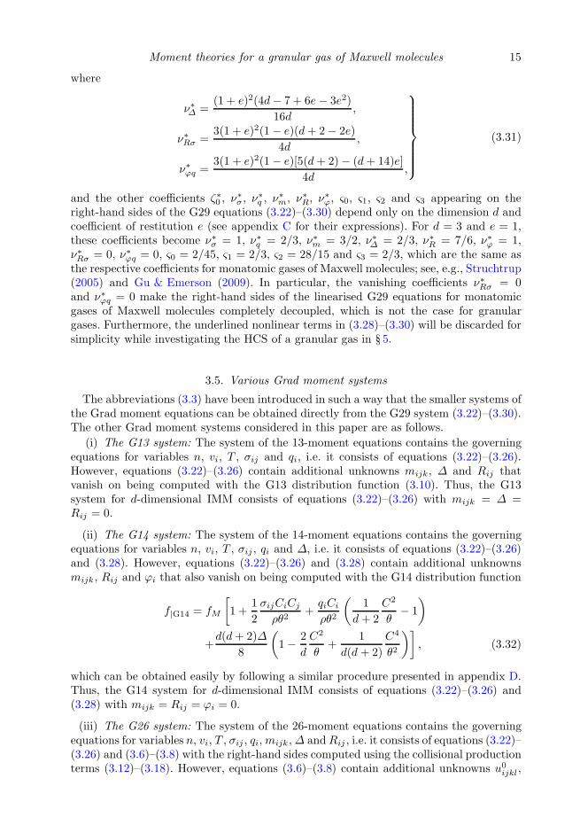
Moment theories for a granular gas of Maxwell molecules 15
where
ν∗∆ =(1 + e)2(4d− 7 + 6e− 3e2)
16d,
ν∗Rσ =3(1 + e)2(1− e)(d+ 2− 2e)
4d,
ν∗ϕq =3(1 + e)2(1− e)[5(d+ 2)− (d+ 14)e]
4d,
(3.31)
and the other coefficients ζ∗0 , ν∗σ, ν
∗q , ν
∗m, ν∗R, ν
∗ϕ, ς0, ς1, ς2 and ς3 appearing on the
right-hand sides of the G29 equations (3.22)–(3.30) depend only on the dimension d andcoefficient of restitution e (see appendix C for their expressions). For d = 3 and e = 1,these coefficients become ν∗σ = 1, ν∗q = 2/3, ν∗m = 3/2, ν∗∆ = 2/3, ν∗R = 7/6, ν∗ϕ = 1,ν∗Rσ = 0, ν∗ϕq = 0, ς0 = 2/45, ς1 = 2/3, ς2 = 28/15 and ς3 = 2/3, which are the same asthe respective coefficients for monatomic gases of Maxwell molecules; see, e.g., Struchtrup(2005) and Gu & Emerson (2009). In particular, the vanishing coefficients ν∗Rσ = 0and ν∗ϕq = 0 make the right-hand sides of the linearised G29 equations for monatomicgases of Maxwell molecules completely decoupled, which is not the case for granulargases. Furthermore, the underlined nonlinear terms in (3.28)–(3.30) will be discarded forsimplicity while investigating the HCS of a granular gas in § 5.
3.5. Various Grad moment systems
The abbreviations (3.3) have been introduced in such a way that the smaller systems ofthe Grad moment equations can be obtained directly from the G29 system (3.22)–(3.30).The other Grad moment systems considered in this paper are as follows.
(i) The G13 system: The system of the 13-moment equations contains the governingequations for variables n, vi, T , σij and qi, i.e. it consists of equations (3.22)–(3.26).However, equations (3.22)–(3.26) contain additional unknowns mijk, ∆ and Rij thatvanish on being computed with the G13 distribution function (3.10). Thus, the G13system for d-dimensional IMM consists of equations (3.22)–(3.26) with mijk = ∆ =Rij = 0.
(ii) The G14 system: The system of the 14-moment equations contains the governingequations for variables n, vi, T , σij , qi and ∆, i.e. it consists of equations (3.22)–(3.26)and (3.28). However, equations (3.22)–(3.26) and (3.28) contain additional unknownsmijk, Rij and ϕi that also vanish on being computed with the G14 distribution function
f|G14 = fM
[
1 +1
2
σijCiCj
ρθ2+qiCi
ρθ2
(
1
d+ 2
C2
θ− 1
)
+d(d+ 2)∆
8
(
1− 2
d
C2
θ+
1
d(d + 2)
C4
θ2
)]
, (3.32)
which can be obtained easily by following a similar procedure presented in appendix D.Thus, the G14 system for d-dimensional IMM consists of equations (3.22)–(3.26) and(3.28) with mijk = Rij = ϕi = 0.
(iii) The G26 system: The system of the 26-moment equations contains the governingequations for variables n, vi, T , σij , qi,mijk,∆ andRij , i.e. it consists of equations (3.22)–(3.26) and (3.6)–(3.8) with the right-hand sides computed using the collisional productionterms (3.12)–(3.18). However, equations (3.6)–(3.8) contain additional unknowns u0ijkl,
16 Vinay Kumar Gupta
ϕi and u1ijk that are computed with the G26 distribution function
f|G26 = fM
[
1 +1
2
σijCiCj
ρθ2+qiCi
ρθ2
(
1
d+ 2
C2
θ− 1
)
+1
6
mijkCiCjCk
ρθ3
+d(d+ 2)∆
8
(
1− 2
d
C2
θ+
1
d(d + 2)
C4
θ2
)
+1
4
RijCiCj
ρθ3
(
1
d+ 4
C2
θ− 1
)]
,
(3.33)
which can also be obtained easily by following a similar procedure presented in ap-pendix D. With the G26 distribution function (3.33), u0ijkl and ϕi vanish and u1ijk turns
out to be u1ijk|G26 = (d + 6) θmijk, which is exactly the same as the value of u1ijkobtained with the G29 distribution function (3.20). Therefore, inserting the G26 closure(i.e. u0ijkl = ϕi = 0 and u1ijk = (d+6) θmijk), equations (3.6)–(3.8) turn to (3.27)–(3.29)in which ϕi = 0. Thus, the G26 system for d-dimensional IMM consists of equations(3.22)–(3.29) with ϕi = 0.It is worthwhile to note that the G13 and G26 theories belong to the category of
ordered moment theories, which always include the neglected fluxes of a moment theoryat the previous level (Torrilhon 2015). Also, there are other moment theories, whichconsider complete (traces and traceless) moments of a given order; such moment theoriesare referred to as full moment theories (Torrilhon 2015). The first few examples of fullmoment theories are the Grad 10-, 20- and 35-moment theories (in three dimensions). Inthis sense, the G14 and G29 theories considered in the present work neither belong tothe category of ordered moment theories nor to that of full moment theories.
4. Transport coefficients in the NSF laws
Recall that system (2.8)–(2.10) of the mass, momentum and energy balance equationswas not closed due to the presence of additional unknowns: the stress σij , heat flux qiand cooling rate ζ. One of the major goals of kinetic theory is to furnish a closure for thesystem of the mass, momentum and energy balance equations in the form of constitutiverelations. Traditionally, these constitutive relations are derived by performing the CEexpansion on the Boltzmann equation. An alternative, but relatively much easier, wayto determine the constitutive relations is by means of a CE-like expansion—in powersof a small parameter (usually, the Knudsen number)—performed on the Grad momentsystem. For monatomic gases of Maxwell molecules, it can be shown via the order ofmagnitude approach that a CE-like expansion on the G13 equations yields the Euler, NSFand Burnett constitutive relations at the zeroth, first and second orders of expansion,respectively (Struchtrup 2005). Thus, for monatomic gases of Maxwell molecules, the G13equations already contain the Burnett equations. Such a CE-like expansion procedure ofStruchtrup (2005) on the Grad moment equations for IMM is much more involved dueto non-conservation of energy, and—at its present understanding—does not yield thecorrect transport coefficients appearing in the constitutive relations. I still believe thata formal CE-like expansion procedure based on the order of magnitude of moments,which would yield the correct transport coefficients for granular gases (in particular, forIMM) can be devised; although it will be a topic for future research. Here, I follow theapproach of Garzo (2013) to determine the transport coefficients in the NSF laws for adilute granular gas of IMM through the Grad moment equations developed above.The cooling rate in the energy balance equation (2.10) for IMM is given by (3.19) while
the constitutive relations for the stress and heat flux for closing the system of the mass,momentum and energy balance equations (2.8)–(2.10)—to the linear approximation in
Moment theories for a granular gas of Maxwell molecules 17
spatial gradients—read (Jenkins & Richman 1985a,b; Garzo & Dufty 1999; Garzo 2013)
σij = −2η∂v〈i
∂xj〉, (4.1a)
qi = −κ ∂T∂xi
− λ∂n
∂xi, (4.1b)
where η, κ and λ are the transport coefficients. The coefficient η is referred to asthe shear viscosity and κ as the thermal conductivity; the coefficient λ is a Dufour-like coefficient (Alam et al. 2009; Kremer et al. 2014; Shukla et al. 2019) that vanishesidentically for monatomic gases. Equations (4.1a) and (4.1b) are the Navier–Stokes’ lawand the Fourier’s law for granular gases, respectively. Equations (4.1a) and (4.1b) togetherare referred to as the NSF laws for granular gases.
4.1. Zeroth-order contributions in spatial gradients
To zeroth order in the spatial gradients, the mass, momentum and energy balanceequations (3.22)–(3.24) reduce to
∂n
∂t= 0,
∂vi∂t
= 0 and∂T
∂t= −ζ∗0 ν T (4.2)
while the balance equations for the other higher moments (eqs. (3.25)–(3.30)) reduce to
σij = 0, qi = 0, mijk = 0, ∆− 6(1− e)2
4d− 7 + 6e− 3e2= 0,
ν∗RRij − ν∗Rσθσij = 0, ν∗ϕ ϕi − ν∗ϕqθqi = 0.
(4.3)
Equations in (4.3) readily imply that
σij = qi = mijk = Rij = ϕi = 0 and ∆ = a2. (4.4)
where
a2 =6(1− e)2
4d− 7 + 6e− 3e2(4.5)
is the same as the value of the fourth cumulant for IMM reported in previous studies(Santos 2003; Khalil et al. 2014). Thus, to zeroth order in spatial gradients, σij , qi, mijk,Rij and ϕi are zero while ∆ = a2.
4.2. First-order contributions in spatial gradients
Now, the terms having first-order spatial derivatives are also retained in the momentequations. To first order in spatial gradients, moment equations (3.22)–(3.26), read
∂n
∂t= −vi
∂n
∂xi− n
∂vi∂xi
, (4.6)
∂vi∂t
= −vj∂vi∂xj
− 1
mn
∂(nT )
∂xi, (4.7)
∂T
∂t= −vi
∂T
∂xi− 2
dT∂vi∂xi
− ζ T, (4.8)
∂σij∂t
= −2ρθ∂v〈i
∂xj〉− ν∗σ ν σij , (4.9)
∂qi∂t
= −d+ 2
2
[
a2θ2 ∂ρ
∂xi+ (1 + 2a2)ρθ
∂θ
∂xi
]
− ν∗q ν qi. (4.10)
18 Vinay Kumar Gupta
Notice that, unlike IHS (see Gupta et al. (2018)), here none of the balance equations(3.27)–(3.30) is required for determining the transport coefficients for IMM up to first-order accuracy in spatial gradients, since the stress and heat flux balance equations(eqs. (4.9) and (4.10)) have no coupling with the higher moments. The balance equations(3.27)–(3.30) will only be needed for computing the transport coefficients beyond thefirst-order accuracy in spatial gradients, which is not the focus of the present work.
The time derivatives of the stress and heat flux in (4.9) and (4.10) are computed usingdimensional analysis and using the zeroth-order accurate mass, momentum and energybalance equations (4.2). They turn out to be (Garzo 2013; Gupta et al. 2018)
∂σij∂t
= η ζ∂v〈i
∂xj〉and
∂qi∂t
= 2κ ζ∂T
∂xi+
(
κT
n+
3
2λ
)
ζ∂n
∂xi. (4.11)
Now, in the first-order accurate stress and heat flux balance equations ((4.9) and (4.10)),one replaces σij and qi using (4.1) and their time derivatives using (4.11). Subsequentcomparison of the coefficients of each hydrodynamic gradient in both the resultingequations leads to the transport coefficients in the NSF laws (4.1):
η = η0 η∗, κ = κ0 κ
∗ and λ =κ0 T
nλ∗ (4.12)
where
η0 =nT
νand κ0 =
d(d + 2)
2(d− 1)mη0 (4.13)
are the shear viscosity and thermal conductivity, respectively, in the elastic limit; andη∗, κ∗ and λ∗ are the reduced shear viscosity, reduced thermal conductivity and reducedDufour-like coefficient, respectively. These reduced transport coefficients are given by
η∗ =1
ν∗σ − 12ζ
∗0
, (4.14a)
κ∗ =d− 1
d
1 + 2 a2ν∗q − 2ζ∗0
, (4.14b)
λ∗ =κ∗ζ∗0 + d−1
d a2
ν∗q − 32ζ
∗0
=κ∗
1 + 2a2
ζ∗0 + ν∗q a2
ν∗q − 32ζ
∗0
. (4.14c)
Expressions (4.14) for the reduced transport coefficients agree with those obtained atfirst order of the CE expansion for IMM, e.g. in Santos (2003); Khalil et al. (2014);Garzo & Santos (2011). Indeed, the structure of these transport coefficients is very similarto those for IHS (Brey et al. 1998a; Garzo 2013) except for the fact that a2, ζ
∗0 , ν
∗σ and ν∗q
for IMM and IHS are different. Despite the structural similarity, the transport coefficientsκ∗ and λ∗ for IMM ((4.14b) and (4.14c)) diverge at a certain value of the coefficient ofrestitution and do not yield meaningful values below it—in contrast to the transportcoefficients for IHS which are meaningful for all values of the coefficient of restitutionand are in reasonably good agreement with the simulations. This issue pertaining toIMM can readily be appreciated by inspecting the explicit dependence of the reducedtransport coefficients on the coefficient of restitution and dimension as follows. Insertinga2, ζ
∗0 , ν
∗σ and ν∗q from (4.5), (C 1), (C 2) and (C 3) in the reduced transport coefficients
(4.14), they are expressed as a function of the coefficient of restitution and dimension
Moment theories for a granular gas of Maxwell molecules 19
(Garzo & Santos 2011):
η∗ =8d
(1 + e)[3d+ 2 + (d− 2)e], (4.15a)
κ∗ =8(d− 1)(4d+ 5− 18e+ 9e2)
(1 + e)(d− 4 + 3de)(4d− 7 + 6e− 3e2), (4.15b)
λ∗ =16(1− e)[2d2 + 8d− 1− 6(d+ 2)e+ 9e2]
(1 + e)2(d− 4 + 3de)(4d− 7 + 6e− 3e2). (4.15c)
Clearly, both κ∗ and λ∗ have singularities at e = (4−d)/(3d), for which the denominatorsof both of them vanish. In particular, the denominators of both κ∗ and λ∗ vanish ate = 1/3 for d = 2 and at e = 1/9 for d = 3. Moreover, below the singularities, i.e.for e < (4 − d)/(3d), both κ∗ and λ∗ are negative, which is unphysical. The existenceof these singularities is apparently attributed to the breakdown of hydrodynamics ingranular gases of IMM for e 6 (4 − d)/(3d) due to the lack of time scale separationbetween the kinetic and hydrodynamic parts of the distribution function (Brey et al.2010). Owing to these singularities, it is customary to write the heat flux as a linearcombination of the gradients of T and n
√T instead of its usual representation (4.1b)
(see, e.g., Garzo et al. 2007; Garzo & Santos 2011). The heat flux in the new form reads
qi = −κ′ ∂T∂xi
− λ√T
∂(n√T )
∂xi, where κ′ = κ− λ
n
2T(4.16)
is referred to as the modified thermal conductivity (Garzo et al. 2007). The reducedmodified thermal conductivity κ′∗ = κ′/κ0—using (4.14)–(4.16)—is given by
κ′∗ =d− 1
d
1 + 32a2
ν∗q − 32ζ
∗0
=8(2d+ 1− 6e+ 3e2)
(1 + e)2(4d− 7 + 6e− 3e2). (4.17)
The reduced modified thermal conductivity κ′∗ does not possess the above singularityand hence is finite for all 0 6 e 6 1 and for d = 2, 3.
4.3. Comparison with existing theories and computer simulations
I have not found any simulation data on the transport coefficients for IMM. Therefore,in this subsection, I compare the reduced transport coefficients for IMM obtained abovewith those for IHD (d = 2) and IHS (d = 3) obtained through various theoretical andsimulation methods.The reduced transport coefficients η∗, κ∗, λ∗ and κ′∗ for a dilute granular gas are
plotted over the coefficient of restitution e in figures 1–4, respectively. The left and rightpanels in each figure exhibit the results for d = 2 and d = 3, respectively. The thicksolid (red) line in each figure denotes the result for IMM obtained from (4.14) or (4.15)and (4.17), which have been obtained in this paper through the Grad moment equations.Recall that the reduced transport coefficients for IMM obtained through the momentmethod above are exactly the same as those obtained at first order of the CE expansion(see Santos 2003; Garzo & Santos 2011). Therefore, the thick solid (red) line in each figurealso represents the results for IMM from the first-order CE expansion. The remaininglines and symbols in figures 1–4 depict the results for IHD (in case of d = 2) or forIHS (in case of d = 3). The thin solid (green) and dash-dotted (magenta) lines are theplots for the reduced transport coefficients from Garzo et al. (2007) obtained at the firstSonine and modified first Sonine approximations, respectively, in the CE expansion. Thedashed (black) lines depict the reduced transport coefficients obtained through the G14
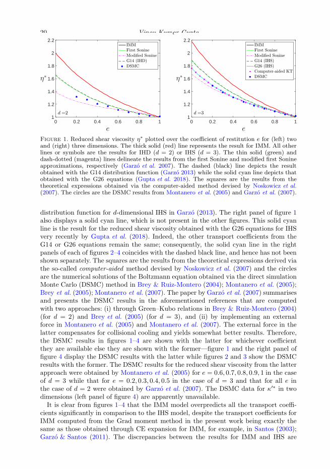
20 Vinay Kumar Gupta
0 0.2 0.4 0.6 0.8 11
1.2
1.4
1.6
1.8
2
2.2
0 0.2 0.4 0.6 0.8 11
1.2
1.4
1.6
1.8
2
2.2
Figure 1. Reduced shear viscosity η∗ plotted over the coefficient of restitution e for (left) twoand (right) three dimensions. The thick solid (red) line represents the result for IMM. All otherlines or symbols are the results for IHD (d = 2) or IHS (d = 3). The thin solid (green) anddash-dotted (magenta) lines delineate the results from the first Sonine and modified first Sonineapproximations, respectively (Garzo et al. 2007). The dashed (black) line depicts the resultobtained with the G14 distribution function (Garzo 2013) while the solid cyan line depicts thatobtained with the G26 equations (Gupta et al. 2018). The squares are the results from thetheoretical expressions obtained via the computer-aided method devised by Noskowicz et al.(2007). The circles are the DSMC results from Montanero et al. (2005) and Garzo et al. (2007).
distribution function for d-dimensional IHS in Garzo (2013). The right panel of figure 1also displays a solid cyan line, which is not present in the other figures. This solid cyanline is the result for the reduced shear viscosity obtained with the G26 equations for IHSvery recently by Gupta et al. (2018). Indeed, the other transport coefficients from theG14 or G26 equations remain the same; consequently, the solid cyan line in the rightpanels of each of figures 2–4 coincides with the dashed black line, and hence has not beenshown separately. The squares are the results from the theoretical expressions derived viathe so-called computer-aided method devised by Noskowicz et al. (2007) and the circlesare the numerical solutions of the Boltzmann equation obtained via the direct simulationMonte Carlo (DSMC) method in Brey & Ruiz-Montero (2004); Montanero et al. (2005);Brey et al. (2005); Montanero et al. (2007). The paper by Garzo et al. (2007) summarisesand presents the DSMC results in the aforementioned references that are computedwith two approaches: (i) through Green–Kubo relations in Brey & Ruiz-Montero (2004)(for d = 2) and Brey et al. (2005) (for d = 3), and (ii) by implementing an externalforce in Montanero et al. (2005) and Montanero et al. (2007). The external force in thelatter compensates for collisional cooling and yields somewhat better results. Therefore,the DSMC results in figures 1–4 are shown with the latter for whichever coefficientthey are available else they are shown with the former—figure 1 and the right panel offigure 4 display the DSMC results with the latter while figures 2 and 3 show the DSMCresults with the former. The DSMC results for the reduced shear viscosity from the latterapproach were obtained by Montanero et al. (2005) for e = 0.6, 0.7, 0.8, 0.9, 1 in the caseof d = 3 while that for e = 0.2, 0.3, 0.4, 0.5 in the case of d = 3 and that for all e inthe case of d = 2 were obtained by Garzo et al. (2007). The DSMC data for κ′∗ in twodimensions (left panel of figure 4) are apparently unavailable.It is clear from figures 1–4 that the IMM model overpredicts all the transport coeffi-
cients significantly in comparison to the IHS model, despite the transport coefficients forIMM computed from the Grad moment method in the present work being exactly thesame as those obtained through CE expansion for IMM, for example, in Santos (2003);Garzo & Santos (2011). The discrepancies between the results for IMM and IHS are
Moment theories for a granular gas of Maxwell molecules 21
0 0.2 0.4 0.6 0.8 11
10
100
400
0 0.2 0.4 0.6 0.8 11
10
100
400
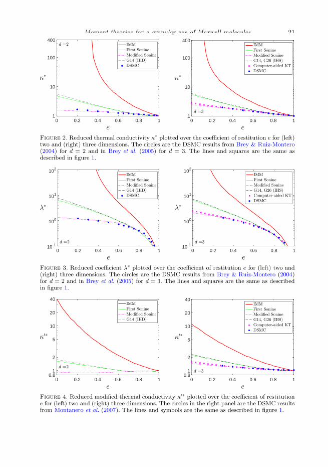
Figure 2. Reduced thermal conductivity κ∗ plotted over the coefficient of restitution e for (left)two and (right) three dimensions. The circles are the DSMC results from Brey & Ruiz-Montero(2004) for d = 2 and in Brey et al. (2005) for d = 3. The lines and squares are the same asdescribed in figure 1.
0 0.2 0.4 0.6 0.8 110-1
100
101
102
0 0.2 0.4 0.6 0.8 110-1
100
101
102
Figure 3. Reduced coefficient λ∗ plotted over the coefficient of restitution e for (left) two and(right) three dimensions. The circles are the DSMC results from Brey & Ruiz-Montero (2004)for d = 2 and in Brey et al. (2005) for d = 3. The lines and squares are the same as describedin figure 1.
0 0.2 0.4 0.6 0.8 10.8
1
2
5
10
20
40
0 0.2 0.4 0.6 0.8 10.8
1
2
5
10
20
40
Figure 4. Reduced modified thermal conductivity κ′∗ plotted over the coefficient of restitutione for (left) two and (right) three dimensions. The circles in the right panel are the DSMC resultsfrom Montanero et al. (2007). The lines and symbols are the same as described in figure 1.
22 Vinay Kumar Gupta
apparently linked to the choice of the effective collision frequency ν (see (2.3a)) in theIMM model (Santos 2003), which is chosen in such a way that the cooling rates fromthe Boltzmann equation for IHS and IMM remain exactly the same. Furthermore, thereduced transport coefficients κ∗ and λ∗ for IMM (shown by the thick solid red lines infigures 2 and 3) diverge at e = 1/3 for d = 2 (left panels of figures 2 and 3) and ate = 1/9 for d = 3 (right panels of figures 2 and 3), and remain unphysical below thesevalues of the coefficient of restitution. On the other hand, the reduced modified thermalconductivity κ′∗ for IMM remains positive for all values of the coefficient of restitution inboth dimensions (see figure 4). Nevertheless, κ′∗ for IMM is also much higher than thatfor IHS. In the case of d = 2 (left panel of figure 4), κ′∗ for IHS from any theory firstdecreases then increases on increasing the coefficient of restitution (although the profilesof κ′∗ from the modified first Sonine approximation and first Sonine approximation/G14theory differ significantly) whereas that for IMM decreases monotonically on increasingthe coefficient of restitution. However, as the DSMC data are not available in this case,it is difficult to discern which theory for IHS yields better results in this case.
Among fully theoretical methods, the modified version of the first Sonine approxima-tion (dash-dotted magenta lines) proposed by Garzo et al. (2007) for IHS seems to bethe best model, which captures all the transport coefficient very well, although the G26model of Gupta et al. (2018) was able to capture the coefficient of the reduced shearviscosity (but not the other transport coefficients) better than the modified first Sonineapproximation.
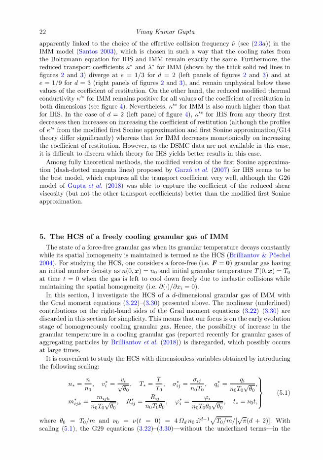
5. The HCS of a freely cooling granular gas of IMM
The state of a force-free granular gas when its granular temperature decays constantlywhile its spatial homogeneity is maintained is termed as the HCS (Brilliantov & Poschel2004). For studying the HCS, one considers a force-free (i.e. F = 0) granular gas havingan initial number density as n(0,x) = n0 and initial granular temperature T (0,x) = T0at time t = 0 when the gas is left to cool down freely due to inelastic collisions whilemaintaining the spatial homogeneity (i.e. ∂(·)/∂xi = 0).
In this section, I investigate the HCS of a d-dimensional granular gas of IMM withthe Grad moment equations (3.22)–(3.30) presented above. The nonlinear (underlined)contributions on the right-hand sides of the Grad moment equations (3.22)–(3.30) arediscarded in this section for simplicity. This means that our focus is on the early evolutionstage of homogeneously cooling granular gas. Hence, the possibility of increase in thegranular temperature in a cooling granular gas (reported recently for granular gases ofaggregating particles by Brilliantov et al. (2018)) is disregarded, which possibly occursat large times.
It is convenient to study the HCS with dimensionless variables obtained by introducingthe following scaling:
n∗ =n
n0, v∗i =
vi√θ0, T∗ =
T
T0, σ∗
ij =σijn0T0
, q∗i =qi
n0T0√θ0,
m∗ijk =
mijk
n0T0√θ0, R∗
ij =Rij
n0T0θ0, ϕ∗
i =ϕi
n0T0θ0√θ0, t∗ = ν0t,
(5.1)
where θ0 = T0/m and ν0 = ν(t = 0) = 4Ωd n0 dd−1√
T0/m/[√π(d + 2)]. With
scaling (5.1), the G29 equations (3.22)–(3.30)—without the underlined terms—in the
Moment theories for a granular gas of Maxwell molecules 23
HCS (i.e. with ∂(·)/∂xi = 0, F = 0) reduce to
dn∗
dt∗= 0, (5.2)
dv∗idt∗
= 0, (5.3)
dT∗dt∗
= −ζ∗0 n∗T3/2∗ , (5.4)
dσ∗ij
dt∗= −ν∗σ n∗
√
T∗ σ∗ij , (5.5)
dq∗idt∗
= −ν∗q n∗
√
T∗ q∗i , (5.6)
dm∗ijk
dt∗= −ν∗m n∗
√
T∗m∗ijk, (5.7)
d∆
dt∗= −ν∗∆ n∗
√
T∗ (∆− a2), (5.8)
dR∗ij
dt∗= −n∗
√
T∗(
ν∗RR∗ij − ν∗RσT∗σ
∗ij
)
, (5.9)
dϕ∗i
dt∗= −n∗
√
T∗(
ν∗ϕϕ∗i − ν∗ϕqT∗q
∗i
)
. (5.10)
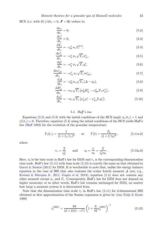
5.1. Haff’s law
Equations (5.2) and (5.3) with the initial conditions of the HCS imply n∗(t∗) = 1 andv∗i (t∗) = 0. Therefore, equation (5.4) using the initial conditions of the HCS yields Haff’slaw (Haff 1983) for the evolution of the granular temperature:
T∗(t∗) =1
(1 + t∗/τ∗)2or T (t) =
T0(1 + t/τ0)2
, (5.11a,b)
where
τ∗ =2
ζ∗0and τ0 =
τ∗ν0
=2
ζ∗0ν0. (5.12a,b)
Here, τ0 is the time scale in Haff’s law for IMM and τ∗ is the corresponding dimensionlesstime scale. Haff’s law (5.11) with time scale (5.12) is exactly the same as that obtained inGarzo & Santos (2011) for IMM. It is worthwhile to note that, unlike the energy balanceequation in the case of IHS that also contains the scalar fourth moment ∆ (see, e.g.,Kremer & Marques Jr. 2011; Gupta et al. 2018), equation (5.4) does not contain anyother moment except n∗ and T∗. Consequently, Haff’s law for IMM does not depend onhigher moments; or in other words, Haff’s law remains unchanged for IMM, no matterhow large a moment system it is determined from.
Note that the dimensionless time scale τ∗ in Haff’s law (5.11) for d-dimensional IHSobtained at first approximation of the Sonine expansion is given by (van Noije & Ernst1998)
τ(IHS)∗ =
8d
(d+ 2)(1− e2)
(
1 +3
16a(IHS)2
)−1
(5.13)
24 Vinay Kumar Gupta
0 10 20 30 40 500
0.2
0.4
0.6
0.8
1
0 10 20 30 40 500
0.2
0.4
0.6
0.8
1
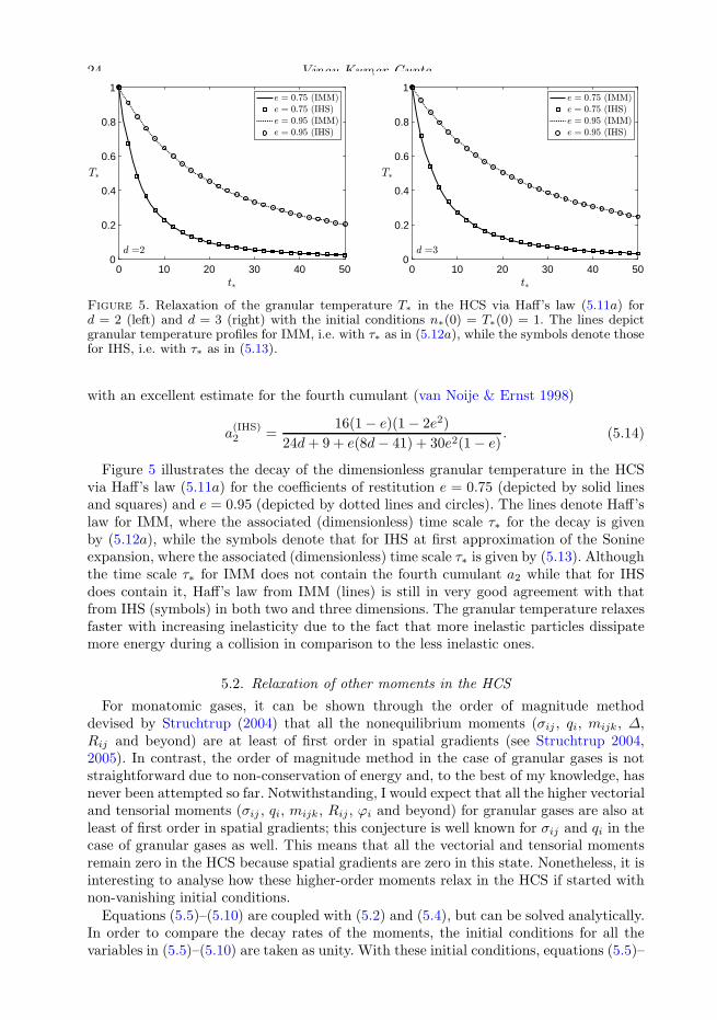
Figure 5. Relaxation of the granular temperature T∗ in the HCS via Haff’s law (5.11a) ford = 2 (left) and d = 3 (right) with the initial conditions n∗(0) = T∗(0) = 1. The lines depictgranular temperature profiles for IMM, i.e. with τ∗ as in (5.12a), while the symbols denote thosefor IHS, i.e. with τ∗ as in (5.13).
with an excellent estimate for the fourth cumulant (van Noije & Ernst 1998)
a(IHS)2 =
16(1− e)(1− 2e2)
24d+ 9 + e(8d− 41) + 30e2(1− e). (5.14)
Figure 5 illustrates the decay of the dimensionless granular temperature in the HCSvia Haff’s law (5.11a) for the coefficients of restitution e = 0.75 (depicted by solid linesand squares) and e = 0.95 (depicted by dotted lines and circles). The lines denote Haff’slaw for IMM, where the associated (dimensionless) time scale τ∗ for the decay is givenby (5.12a), while the symbols denote that for IHS at first approximation of the Sonineexpansion, where the associated (dimensionless) time scale τ∗ is given by (5.13). Althoughthe time scale τ∗ for IMM does not contain the fourth cumulant a2 while that for IHSdoes contain it, Haff’s law from IMM (lines) is still in very good agreement with thatfrom IHS (symbols) in both two and three dimensions. The granular temperature relaxesfaster with increasing inelasticity due to the fact that more inelastic particles dissipatemore energy during a collision in comparison to the less inelastic ones.
5.2. Relaxation of other moments in the HCS
For monatomic gases, it can be shown through the order of magnitude methoddevised by Struchtrup (2004) that all the nonequilibrium moments (σij , qi, mijk, ∆,Rij and beyond) are at least of first order in spatial gradients (see Struchtrup 2004,2005). In contrast, the order of magnitude method in the case of granular gases is notstraightforward due to non-conservation of energy and, to the best of my knowledge, hasnever been attempted so far. Notwithstanding, I would expect that all the higher vectorialand tensorial moments (σij , qi, mijk, Rij , ϕi and beyond) for granular gases are also atleast of first order in spatial gradients; this conjecture is well known for σij and qi in thecase of granular gases as well. This means that all the vectorial and tensorial momentsremain zero in the HCS because spatial gradients are zero in this state. Nonetheless, it isinteresting to analyse how these higher-order moments relax in the HCS if started withnon-vanishing initial conditions.Equations (5.5)–(5.10) are coupled with (5.2) and (5.4), but can be solved analytically.
In order to compare the decay rates of the moments, the initial conditions for all thevariables in (5.5)–(5.10) are taken as unity. With these initial conditions, equations (5.5)–
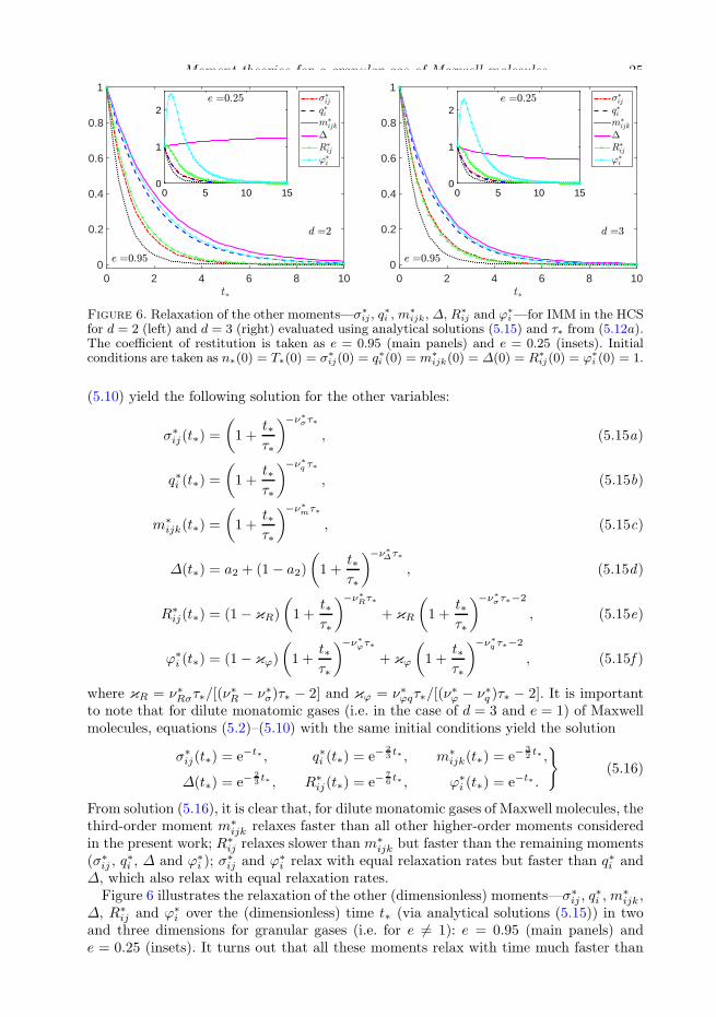
Moment theories for a granular gas of Maxwell molecules 25
0 2 4 6 8 100
0.2
0.4
0.6
0.8
1
0 5 10 150
1
2
0 2 4 6 8 100
0.2
0.4
0.6
0.8
1
0 5 10 150
1
2
Figure 6. Relaxation of the other moments—σ∗
ij , q∗
i , m∗
ijk, ∆, R∗
ij and ϕ∗
i—for IMM in the HCSfor d = 2 (left) and d = 3 (right) evaluated using analytical solutions (5.15) and τ∗ from (5.12a).The coefficient of restitution is taken as e = 0.95 (main panels) and e = 0.25 (insets). Initialconditions are taken as n∗(0) = T∗(0) = σ∗
ij(0) = q∗i (0) = m∗
ijk(0) = ∆(0) = R∗
ij(0) = ϕ∗
i (0) = 1.
(5.10) yield the following solution for the other variables:
σ∗ij(t∗) =
(
1 +t∗τ∗
)−ν∗
στ∗
, (5.15a)
q∗i (t∗) =
(
1 +t∗τ∗
)−ν∗
q τ∗
, (5.15b)
m∗ijk(t∗) =
(
1 +t∗τ∗
)−ν∗
mτ∗
, (5.15c)
∆(t∗) = a2 + (1− a2)
(
1 +t∗τ∗
)−ν∗
∆τ∗
, (5.15d)
R∗ij(t∗) = (1− κR)
(
1 +t∗τ∗
)−ν∗
Rτ∗
+ κR
(
1 +t∗τ∗
)−ν∗
στ∗−2
, (5.15e)
ϕ∗i (t∗) = (1− κϕ)
(
1 +t∗τ∗
)−ν∗
ϕτ∗
+ κϕ
(
1 +t∗τ∗
)−ν∗
q τ∗−2
, (5.15f )
where κR = ν∗Rστ∗/[(ν∗R − ν∗σ)τ∗ − 2] and κϕ = ν∗ϕqτ∗/[(ν
∗ϕ − ν∗q )τ∗ − 2]. It is important
to note that for dilute monatomic gases (i.e. in the case of d = 3 and e = 1) of Maxwellmolecules, equations (5.2)–(5.10) with the same initial conditions yield the solution
σ∗ij(t∗) = e−t∗ , q∗i (t∗) = e−
23t∗ , m∗
ijk(t∗) = e−32t∗ ,
∆(t∗) = e−23t∗ , R∗
ij(t∗) = e−76t∗ , ϕ∗
i (t∗) = e−t∗ .
(5.16)
From solution (5.16), it is clear that, for dilute monatomic gases of Maxwell molecules, thethird-order moment m∗
ijk relaxes faster than all other higher-order moments consideredin the present work; R∗
ij relaxes slower than m∗ijk but faster than the remaining moments
(σ∗ij , q
∗i , ∆ and ϕ∗
i ); σ∗ij and ϕ∗
i relax with equal relaxation rates but faster than q∗i and∆, which also relax with equal relaxation rates.Figure 6 illustrates the relaxation of the other (dimensionless) moments—σ∗
ij , q∗i ,m
∗ijk,
∆, R∗ij and ϕ∗
i over the (dimensionless) time t∗ (via analytical solutions (5.15)) in twoand three dimensions for granular gases (i.e. for e 6= 1): e = 0.95 (main panels) ande = 0.25 (insets). It turns out that all these moments relax with time much faster than
26 Vinay Kumar Gupta
the granular temperature. It is interesting to note that all the vectorial and tensorialmoments relax to zero whereas the scalar moment ∆ relaxes to a nonzero value a2 forall e 6= 1. These can also be verified from analytical solutions (5.15) in the limit t∗ → ∞,since all the exponents in (5.15) are negative for all e 6= 1 (note that τ∗, ν
∗σ, ν
∗q , ν
∗m,
ν∗∆, ν∗R, ν∗Rσ, ν
∗ϕ, ν
∗ϕq, α0, α1, α2 and α3 are positive for e 6= 1). For large values of the
coefficient of restitution (main panels), all these moments decay monotonically and theirdecay rates are, apparently, proportional to their tensorial orders, i.e. the third-ordermoment (m∗
ijk) decays faster than the second-order moments (σ∗ij and R∗
ij), which decayfaster than the vectorial moment (q∗i and ϕ∗
i ), which decay faster than the scalar moment(∆). However, for sufficiently small values of the coefficient of restitution (insets), thehigher-order moments (R∗
ij and ϕ∗i ) do not decay monotonically. This is attributed to the
fact that higher-order (sixth-order and beyond) moments for IMM are prone to divergefor sufficiently small values of the coefficient of restitution in the HCS (Santos & Garzo2012) and it is manifested already through the non-monotonic relaxation of R∗
ij and ϕ∗i
for small coefficients of restitution (insets), although they themselves do not diverge.
6. Linear stability analysis of the HCS
In this section, the temporal stability of the HCS of a freely cooling granular gasof IMM due to small perturbations will be analysed through the G29 and other Gradmoment theories described in § 3.5 with Fi = 0. The amplitudes of these perturbationsare assumed to be sufficiently small in order to ensure the validity of the linear analysis.
For the linear stability analysis, all the field variables in (3.22)–(3.30) are decomposedinto their reference state values (i.e. their solutions in the HCS) plus perturbations fromtheir respective reference state values. In other words, the field variables in the G29system (3.22)–(3.30) are written as
n(t,x) = n0
[
1 + n(t,x)]
, (6.1a)
vi(t,x) = vH(t) vi(t,x), (6.1b)
T (t,x) = TH(t)[
1 + T (t,x)]
, (6.1c)
σij(t,x) = n0 TH(t) σij(t,x), (6.1d)
qi(t,x) = n0 TH(t) vH(t) qi(t,x), (6.1e)
mijk(t,x) = n0 TH(t) vH(t) mijk(t,x), (6.1f )
∆(t,x) = a2 + ∆(t,x), (6.1g)
Rij(t,x) = n0 TH(t) vH(t)2 Rij(t,x), (6.1h)
ϕi(t,x) = n0 TH(t) vH(t)3 ϕi(t,x), (6.1i)
where TH(t) is the granular temperature in the HCS and vH(t) =√
TH(t)/m is a refer-ence speed proportional to the adiabatic sound speed in the HCS; and the quantities withtilde denote the dimensionless perturbations in the field variables from their respectivesolutions in the HCS.
Inserting expressions (6.1) for the field variables into (3.22)–(3.30) and discarding allthe nonlinear terms of the perturbations, one obtains the system of linear PDEs in(dimensionless) perturbed field variables with time-dependent coefficients. This systemof PDEs is transformed to a new system of PDEs having time-independent coefficients
Moment theories for a granular gas of Maxwell molecules 27
by introducing a length scale
ℓ :=vH(t)
νH(t), where νH(t) =
4Ωd√π(d+ 2)
n0dd−1
√
TH(t)
m, (6.2)
that is employed to make the space variables dimensionless (i.e. xi = xi/ℓ, where tildedenotes the dimensionless space variable), and a dimensionless time
t :=
∫ t
0
νH(t′) dt′ (6.3)
that measures time as the number of effective collisions per particle (Brey et al. 1998b;Brilliantov & Poschel 2004; Garzo & Santos 2007). The resulting system of PDEs havingtime-independent coefficients reads
∂n
∂t+∂vi∂xi
= 0, (6.4)
∂vi
∂t+∂σij∂xj
+∂n
∂xi+∂T
∂xi− 1
2ζ∗0 vi = 0, (6.5)
∂T
∂t+
2
d
(
∂qi∂xi
+∂vi∂xi
)
+ ζ∗0
(
n+1
2T
)
= 0, (6.6)
∂σij
∂t+∂mijk
∂xk+
4
d+ 2
∂q〈i
∂xj〉+ 2
∂v〈i
∂xj〉+ ξσσij = 0, (6.7)
∂qi
∂t+
1
2
∂Rij
∂xj+∂σij∂xj
+d+ 2
2
[
∂∆
∂xi+ a2
∂n
∂xi+ (1 + 2a2)
∂T
∂xi
]
+ ξq qi = 0, (6.8)
∂mijk
∂t+
3
d+ 4
∂R〈ij
∂xk〉+ 3
∂σ〈ij
∂xk〉+ ξmmijk = 0, (6.9)
∂∆
∂t+ ξ1
∂qi∂xi
+1
d(d+ 2)
∂ϕi
∂xi+ ν∗∆ ∆ = 0, (6.10)
∂Rij
∂t+
2
d+ 2
∂ϕ〈i
∂xj〉+
4(d+ 4)
d+ 2
∂q〈i∂xj〉
+ 2(d+ 4)a2∂v〈i∂xj〉
+ 2∂mijk
∂xk
+ξRRij − ν∗Rσσij = 0, (6.11)
∂ϕi
∂t+ 4
∂Rij
∂xj+ ξ2
(
∂∆
∂xi+ 4a2
∂T
∂xi− a2
∂σij∂xj
)
+ ξϕϕi − ν∗ϕq qi = 0, (6.12)
where
ξσ = ν∗σ − ζ∗0 , ξq = ν∗q − 3
2ζ∗0 , ξm = ν∗m − 3
2ζ∗0 , ξR = ν∗R − 2ζ∗0 ,
ξϕ = ν∗ϕ − 5
2ζ∗0 , ξ1 =
8
d(d+ 2)
(
1− d+ 2
2a2
)
, ξ2 = (d+ 2)(d+ 4).
(6.13)
System (6.4)–(6.12), admits a normal mode solution of the form
Ψ = Ψ exp[
i(k · x− ω t)]
, (6.14)
where Ψ = (n, vi, T , σij , qi, mijk, ∆, Rij , ϕi)T is the vector containing all the dimension-
less perturbations and Ψ = (n, vi, T , σij , qi, mijk, ∆, Rij , ϕi)T the vector containing their
corresponding complex amplitudes. Furthermore, in the normal mode solution (6.14),i is the imaginary unit, k the dimensionless wavevector of the disturbance and ω the
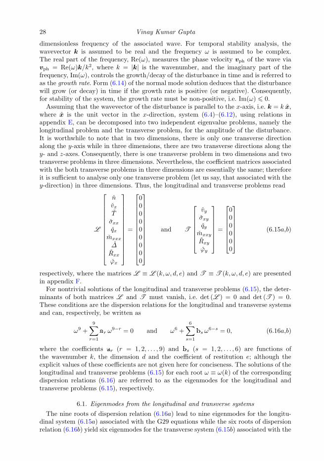
28 Vinay Kumar Gupta
dimensionless frequency of the associated wave. For temporal stability analysis, thewavevector k is assumed to be real and the frequency ω is assumed to be complex.The real part of the frequency, Re(ω), measures the phase velocity vph of the wave viavph = Re(ω)k/k2, where k = |k| is the wavenumber, and the imaginary part of thefrequency, Im(ω), controls the growth/decay of the disturbance in time and is referred toas the growth rate. Form (6.14) of the normal mode solution deduces that the disturbancewill grow (or decay) in time if the growth rate is positive (or negative). Consequently,for stability of the system, the growth rate must be non-positive, i.e. Im(ω) 6 0.Assuming that the wavevector of the disturbance is parallel to the x-axis, i.e. k = k x,
where x is the unit vector in the x-direction, system (6.4)–(6.12), using relations inappendix E, can be decomposed into two independent eigenvalue problems, namely thelongitudinal problem and the transverse problem, for the amplitude of the disturbance.It is worthwhile to note that in two dimensions, there is only one transverse directionalong the y-axis while in three dimensions, there are two transverse directions along they- and z-axes. Consequently, there is one transverse problem in two dimensions and twotransverse problems in three dimensions. Nevertheless, the coefficient matrices associatedwith the both transverse problems in three dimensions are essentially the same; thereforeit is sufficient to analyse only one transverse problem (let us say, that associated with they-direction) in three dimensions. Thus, the longitudinal and transverse problems read
L
nvxTσxxqx
mxxx
∆Rxx
ϕx
=
000000000
and T
vyσxyqy
mxxy
Rxy
ϕy
=
000000
(6.15a,b)
respectively, where the matrices L ≡ L (k, ω, d, e) and T ≡ T (k, ω, d, e) are presentedin appendix F.For nontrivial solutions of the longitudinal and transverse problems (6.15), the deter-
minants of both matrices L and T must vanish, i.e. det (L ) = 0 and det (T ) = 0.These conditions are the dispersion relations for the longitudinal and transverse systemsand can, respectively, be written as
ω9 +
9∑
r=1
ar ω9−r = 0 and ω6 +
6∑
s=1
bs ω6−s = 0, (6.16a,b)
where the coefficients ar (r = 1, 2, . . . , 9) and bs (s = 1, 2, . . . , 6) are functions ofthe wavenumber k, the dimension d and the coefficient of restitution e; although theexplicit values of these coefficients are not given here for conciseness. The solutions of thelongitudinal and transverse problems (6.15) for each root ω ≡ ω(k) of the correspondingdispersion relations (6.16) are referred to as the eigenmodes for the longitudinal andtransverse problems (6.15), respectively.
6.1. Eigenmodes from the longitudinal and transverse systems
The nine roots of dispersion relation (6.16a) lead to nine eigenmodes for the longitu-dinal system (6.15a) associated with the G29 equations while the six roots of dispersionrelation (6.16b) yield six eigenmodes for the transverse system (6.15b) associated with the
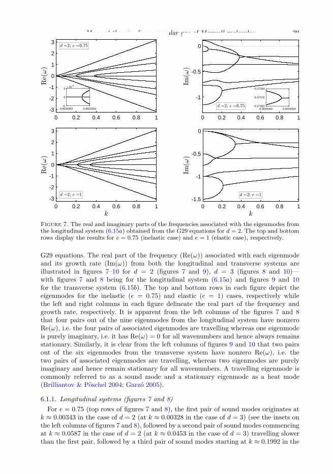
Moment theories for a granular gas of Maxwell molecules 29
0 0.2 0.4 0.6 0.8 1-3
-2
-1
0
1
2
3
0.0034303 0.0034304-5
0
510-5
0 0.2 0.4 0.6 0.8 1
-1
-0.5
0
0.0034303 0.0034304-0.37383
-0.37376
-0.37369
0 0.2 0.4 0.6 0.8 1-3
-2
-1
0
1
2
3
0 0.2 0.4 0.6 0.8 1-1.5
-1
-0.5
0
Figure 7. The real and imaginary parts of the frequencies associated with the eigenmodes fromthe longitudinal system (6.15a) obtained from the G29 equations for d = 2. The top and bottomrows display the results for e = 0.75 (inelastic case) and e = 1 (elastic case), respectively.
G29 equations. The real part of the frequency (Re(ω)) associated with each eigenmodeand its growth rate (Im(ω)) from both the longitudinal and transverse systems areillustrated in figures 7–10 for d = 2 (figures 7 and 9), d = 3 (figures 8 and 10)—with figures 7 and 8 being for the longitudinal system (6.15a) and figures 9 and 10for the transverse system (6.15b). The top and bottom rows in each figure depict theeigenmodes for the inelastic (e = 0.75) and elastic (e = 1) cases, respectively whilethe left and right columns in each figure delineate the real part of the frequency andgrowth rate, respectively. It is apparent from the left columns of the figures 7 and 8that four pairs out of the nine eigenmodes from the longitudinal system have nonzeroRe(ω), i.e. the four pairs of associated eigenmodes are travelling whereas one eigenmodeis purely imaginary, i.e. it has Re(ω) = 0 for all wavenumbers and hence always remainsstationary. Similarly, it is clear from the left columns of figures 9 and 10 that two pairsout of the six eigenmodes from the transverse system have nonzero Re(ω), i.e. thetwo pairs of associated eigenmodes are travelling, whereas two eigenmodes are purelyimaginary and hence remain stationary for all wavenumbers. A travelling eigenmode iscommonly referred to as a sound mode and a stationary eigenmode as a heat mode(Brilliantov & Poschel 2004; Garzo 2005).
6.1.1. Longitudinal systems (figures 7 and 8)
For e = 0.75 (top rows of figures 7 and 8), the first pair of sound modes originates atk ≈ 0.00343 in the case of d = 2 (at k ≈ 0.00328 in the case of d = 3) (see the insets onthe left columns of figures 7 and 8), followed by a second pair of sound modes commencingat k ≈ 0.0587 in the case of d = 2 (at k ≈ 0.0453 in the case of d = 3) travelling slowerthan the first pair, followed by a third pair of sound modes starting at k ≈ 0.1992 in the
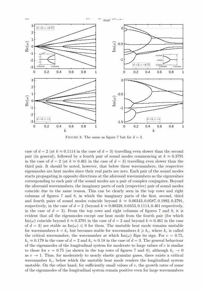
30 Vinay Kumar Gupta
0 0.2 0.4 0.6 0.8 1-3
-2
-1
0
1
2
3
0.0032834 0.0032835-4
-2
0
2
410-5
0 0.2 0.4 0.6 0.8 1
-1
-0.5
0
0.0032834 0.0032835-0.50454
-0.5045
-0.50446
0 0.2 0.4 0.6 0.8 1-3
-2
-1
0
1
2
3
0 0.2 0.4 0.6 0.8 1-1.5
-1
-0.5
0
Figure 8. The same as figure 7 but for d = 3.
case of d = 2 (at k ≈ 0.1114 in the case of d = 3) travelling even slower than the secondpair (in general), followed by a fourth pair of sound modes commencing at k ≈ 0.3791in the case of d = 2 (at k ≈ 0.461 in the case of d = 3) travelling even slower than thethird pair. It should be noted, however, that below these wavenumbers, the respectiveeigenmodes are heat modes since their real parts are zero. Each pair of the sound modesstarts propagating in opposite directions at the aforesaid wavenumbers as the eigenvaluescorresponding to each pair of the sound modes are a pair of complex conjugates. Beyondthe aforesaid wavenumbers, the imaginary parts of each (respective) pair of sound modescoincide due to the same reason. This can be clearly seen in the top rows and rightcolumns of figures 7 and 8, in which the imaginary parts of the first, second, thirdand fourth pairs of sound modes coincide beyond k ≈ 0.00343, 0.0587, 0.1992, 0.3791,respectively, in the case of d = 2 (beyond k ≈ 0.00328, 0.0453, 0.1114, 0.461 respectively,in the case of d = 3). From the top rows and right columns of figures 7 and 8, it isevident that all the eigenmodes except one heat mode from the fourth pair (for whichIm(ω) coincide beyond k ≈ 0.3791 in the case of d = 2 and beyond k ≈ 0.461 in the caseof d = 3) are stable as Im(ω) 6 0 for them. The unstable heat mode remains unstablefor wavenumbers k < kc but becomes stable for wavenumbers k > kc, where kc is calledthe critical wavenumber, the wavenumber at which Im(ω) flips its sign. For e = 0.75,kc ≈ 0.179 in the case of d = 2 and kc ≈ 0.18 in the case of d = 3. The general behaviourof the eigenmodes of the longitudinal system for moderate to large values of e is similarto those for e = 0.75 (as shown in the top rows of figures 7 and 8), although kc → 0as e → 1. Thus, for moderately to nearly elastic granular gases, there exists a criticalwavenumber kc, below which the unstable heat mode renders the longitudinal systemunstable. On the other hand, for sufficiently small values of e, the growth rates of someof the eigenmodes of the longitudinal system remain positive even for large wavenumbers
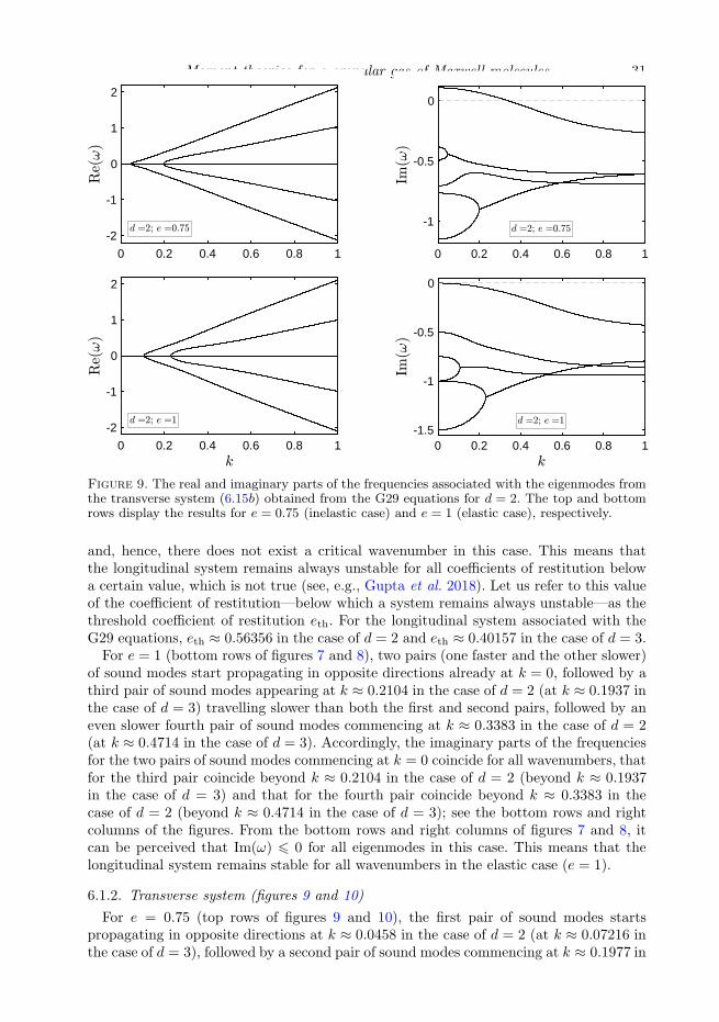
Moment theories for a granular gas of Maxwell molecules 31
0 0.2 0.4 0.6 0.8 1
-2
-1
0
1
2
0 0.2 0.4 0.6 0.8 1
-1
-0.5
0
0 0.2 0.4 0.6 0.8 1
-2
-1
0
1
2
0 0.2 0.4 0.6 0.8 1-1.5
-1
-0.5
0
Figure 9. The real and imaginary parts of the frequencies associated with the eigenmodes fromthe transverse system (6.15b) obtained from the G29 equations for d = 2. The top and bottomrows display the results for e = 0.75 (inelastic case) and e = 1 (elastic case), respectively.
and, hence, there does not exist a critical wavenumber in this case. This means thatthe longitudinal system remains always unstable for all coefficients of restitution belowa certain value, which is not true (see, e.g., Gupta et al. 2018). Let us refer to this valueof the coefficient of restitution—below which a system remains always unstable—as thethreshold coefficient of restitution eth. For the longitudinal system associated with theG29 equations, eth ≈ 0.56356 in the case of d = 2 and eth ≈ 0.40157 in the case of d = 3.For e = 1 (bottom rows of figures 7 and 8), two pairs (one faster and the other slower)
of sound modes start propagating in opposite directions already at k = 0, followed by athird pair of sound modes appearing at k ≈ 0.2104 in the case of d = 2 (at k ≈ 0.1937 inthe case of d = 3) travelling slower than both the first and second pairs, followed by aneven slower fourth pair of sound modes commencing at k ≈ 0.3383 in the case of d = 2(at k ≈ 0.4714 in the case of d = 3). Accordingly, the imaginary parts of the frequenciesfor the two pairs of sound modes commencing at k = 0 coincide for all wavenumbers, thatfor the third pair coincide beyond k ≈ 0.2104 in the case of d = 2 (beyond k ≈ 0.1937in the case of d = 3) and that for the fourth pair coincide beyond k ≈ 0.3383 in thecase of d = 2 (beyond k ≈ 0.4714 in the case of d = 3); see the bottom rows and rightcolumns of the figures. From the bottom rows and right columns of figures 7 and 8, itcan be perceived that Im(ω) 6 0 for all eigenmodes in this case. This means that thelongitudinal system remains stable for all wavenumbers in the elastic case (e = 1).
6.1.2. Transverse system (figures 9 and 10)
For e = 0.75 (top rows of figures 9 and 10), the first pair of sound modes startspropagating in opposite directions at k ≈ 0.0458 in the case of d = 2 (at k ≈ 0.07216 inthe case of d = 3), followed by a second pair of sound modes commencing at k ≈ 0.1977 in
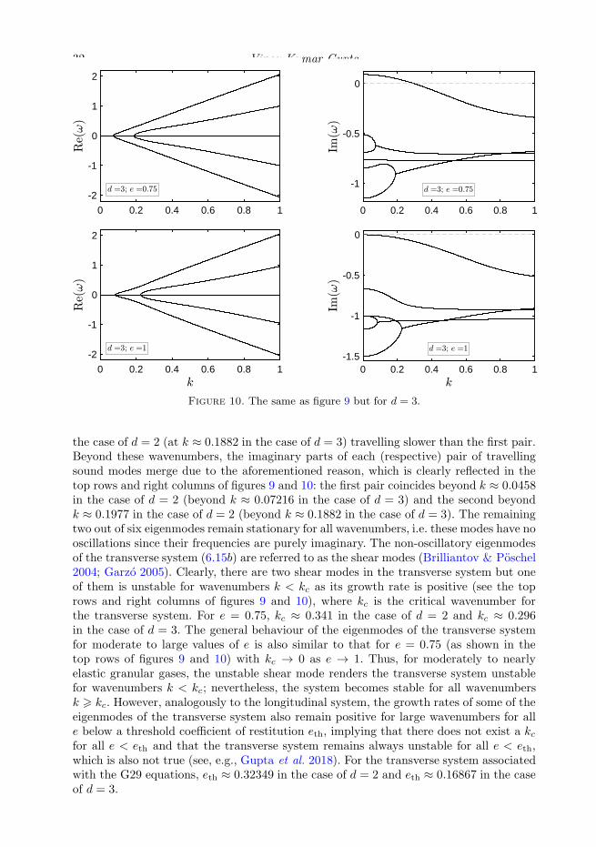
32 Vinay Kumar Gupta
0 0.2 0.4 0.6 0.8 1
-2
-1
0
1
2
0 0.2 0.4 0.6 0.8 1
-1
-0.5
0
0 0.2 0.4 0.6 0.8 1
-2
-1
0
1
2
0 0.2 0.4 0.6 0.8 1-1.5
-1
-0.5
0
Figure 10. The same as figure 9 but for d = 3.
the case of d = 2 (at k ≈ 0.1882 in the case of d = 3) travelling slower than the first pair.Beyond these wavenumbers, the imaginary parts of each (respective) pair of travellingsound modes merge due to the aforementioned reason, which is clearly reflected in thetop rows and right columns of figures 9 and 10: the first pair coincides beyond k ≈ 0.0458in the case of d = 2 (beyond k ≈ 0.07216 in the case of d = 3) and the second beyondk ≈ 0.1977 in the case of d = 2 (beyond k ≈ 0.1882 in the case of d = 3). The remainingtwo out of six eigenmodes remain stationary for all wavenumbers, i.e. these modes have nooscillations since their frequencies are purely imaginary. The non-oscillatory eigenmodesof the transverse system (6.15b) are referred to as the shear modes (Brilliantov & Poschel2004; Garzo 2005). Clearly, there are two shear modes in the transverse system but oneof them is unstable for wavenumbers k < kc as its growth rate is positive (see the toprows and right columns of figures 9 and 10), where kc is the critical wavenumber forthe transverse system. For e = 0.75, kc ≈ 0.341 in the case of d = 2 and kc ≈ 0.296in the case of d = 3. The general behaviour of the eigenmodes of the transverse systemfor moderate to large values of e is also similar to that for e = 0.75 (as shown in thetop rows of figures 9 and 10) with kc → 0 as e → 1. Thus, for moderately to nearlyelastic granular gases, the unstable shear mode renders the transverse system unstablefor wavenumbers k < kc; nevertheless, the system becomes stable for all wavenumbersk > kc. However, analogously to the longitudinal system, the growth rates of some of theeigenmodes of the transverse system also remain positive for large wavenumbers for alle below a threshold coefficient of restitution eth, implying that there does not exist a kcfor all e < eth and that the transverse system remains always unstable for all e < eth,which is also not true (see, e.g., Gupta et al. 2018). For the transverse system associatedwith the G29 equations, eth ≈ 0.32349 in the case of d = 2 and eth ≈ 0.16867 in the caseof d = 3.
Moment theories for a granular gas of Maxwell molecules 33
For e = 1 (bottom rows of figures 9 and 10), the first pair of travelling sound modesstarts propagating in opposite directions at k ≈ 0.1056 in the case of d = 2 (at k ≈0.08398 in the case of d = 3), followed by a second pair of sound modes commencingat k ≈ 0.2296 in the case of d = 2 (at k ≈ 0.22396 in the case of d = 3) travellingslower than the first pair. Accordingly, the imaginary parts of frequencies for the firstpair of travelling sound modes merge beyond k ≈ 0.1056 in the case of d = 2 (beyondk ≈ 0.08398 in the case of d = 3) and that for the second pair merge beyond k ≈ 0.2296in the case of d = 2 (beyond k ≈ 0.22396 in the case of d = 3); see the bottom rows andright columns of the figures. The remaining two eigenmodes are stable shear modes inthe elastic case since the real parts of their associated frequencies are zero and imaginaryparts (growth rates) are non-positive for all wavenumbers. Consequently, the transversesystem also remains stable for all wavenumbers in the elastic case (e = 1).
6.2. Comparison among various Grad moment theories
As discussed in § 3.5, a lower-level Grad moment system can be obtained from the G29equations by discarding the appropriate field variables. Accordingly, the longitudinal andtransverse problems associated with the G13, G14 and G26 systems can be obtained byeliminating the appropriate variables and corresponding rows and columns of the matricesL and T in (6.15). For comparison purpose, I shall also include the results obtainedfrom the linear stability analysis of the system of the NSF equations for IMM along withthese Grad moment systems. The linear-dimensionless NSF equations in the perturbedfield variables are (6.4)–(6.6) with
σij = −2η∗∂v〈i
∂xj〉and qi = −d(d+ 2)
2(d− 1)
(
κ∗∂T
∂xi+ λ∗
∂n
∂xi
)
, (6.17)
where the reduced transport coefficients η∗, κ∗ and λ∗ for IMM are given by (4.14). Fromthe linear-dimensionless NSF equations, it is straightforward to obtain the longitudinaland transverse problems associated with the system of the NSF equations by followinga similar procedure as above. The longitudinal and transverse problems associated withthe system of the NSF equations read
LNSF
nvxT
=
000
and
(
−ω − iη∗k2 + i
ζ∗02
)
vy = 0, (6.18)
respectively, where the matrix LNSF ≡ LNSF(k, ω, d, e) is also presented in appendix F.As far as the linear stability of the HCS is concerned, the NSF theory and all Gradmoment theories—although not shown here explicitly for the NSF, G13, G14 and G26equations—predict a similar behaviour for moderate to large values of the coefficient ofrestitution in the sense that one heat mode from the longitudinal system associated witheach theory and one shear mode from the transverse system associated with each theoryare unstable below some critical wavenumbers for granular gases while all the modesremain stable in the elastic case (e = 1). The stability of a (longitudinal or transverse)system is regulated by its least stable eigenmode. Therefore, to analyse the stability ofthe longitudinal and transverse systems associated with different moment theories, thecritical wavenumbers for the least stable mode (unstable shear mode for the longitudinalsystem and unstable heat mode for the transverse system) from each moment theory areplotted in the (e, kc)-plane in figure 11. The figure also includes the critical wavenumberprofiles (shown by thin dashed black lines) for the least stable modes of the longitudinaland transverse systems associated with the NSF theory for IMM. The top and bottom
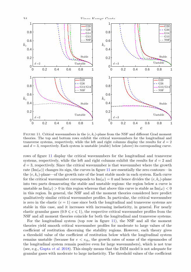
34 Vinay Kumar Gupta
0 0.2 0.4 0.6 0.8 10
0.2
0.4
0.6
0.8
1
0 0.2 0.4 0.6 0.8 10
0.2
0.4
0.6
0.8
1
0 0.2 0.4 0.6 0.8 10
0.2
0.4
0.6
0.8
1
0 0.2 0.4 0.6 0.8 10
0.2
0.4
0.6
0.8
1
Figure 11. Critical wavenumbers in the (e, kc)-plane from the NSF and different Grad momenttheories. The top and bottom rows exhibit the critical wavenumbers for the longitudinal andtransverse systems, respectively, while the left and right columns display the results for d = 2and d = 3, respectively. Each system is unstable (stable) below (above) its corresponding curve.
rows of figure 11 display the critical wavenumbers for the longitudinal and transversesystems, respectively, while the left and right columns exhibit the results for d = 2 andd = 3, respectively. Since the critical wavenumber is that wavenumber where the growthrate (Im(ω)) changes its sign, the curves in figure 11 are essentially the zero contours—inthe (e, kc)-plane—of the growth rate of the least stable mode in each system. Each curvefor the critical wavenumber corresponds to Im(ω) = 0 and hence divides the (e, kc)-planeinto two parts demarcating the stable and unstable regions: the region below a curve isunstable as Im(ω) > 0 in this region whereas that above this curve is stable as Im(ω) < 0in this region. In general, the NSF and all the moment theories considered here predictqualitatively similar critical wavenumber profiles. In particular, the critical wavenumberis zero in the elastic (e = 1) case since both the longitudinal and transverse systems arestable in this case, and it increases with increasing inelasticity, in general. For nearlyelastic granular gases (0.9 6 e 6 1), the respective critical wavenumber profiles from theNSF and all moment theories coincide for both the longitudinal and transverse systems.For the longitudinal system (top row in figure 11), the NSF and all the moment
theories yield smooth critical wavenumber profiles for moderate to large values of thecoefficient of restitution discerning the stability regions. However, each theory givesa threshold value of the coefficient of restitution below which the longitudinal systemremains unstable (because for e < eth, the growth rates of some of the eigenmodes ofthe longitudinal system remain positive even for large wavenumbers), which is not true(see, e.g., Gupta et al. 2018). This simply means that the IMM model is not adequate forgranular gases with moderate to large inelasticity. The threshold values of the coefficient
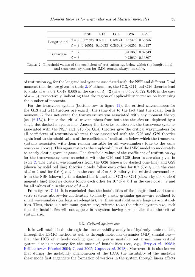
Moment theories for a granular gas of Maxwell molecules 35
NSF G13 G14 G26 G29
Longitudinald = 2 0.62798 0.60211 0.52174 0.37473 0.56356
d = 3 0.46551 0.46033 0.38608 0.06256 0.40157
Transversed = 2 – – – 0.41360 0.32349
d = 3 – – – 0.23030 0.16867
Table 2. Threshold values of the coefficient of restitution eth below which the longitudinaland transverse systems for IMM remain always unstable.
of restitution eth for the longitudinal systems associated with the NSF and different Gradmoment theories are given in table 2. Furthermore, the G13, G14 and G26 theories leadto kinks at e ≈ 0.7, 0.648, 0.608 in the case of d = 2 (at e ≈ 0.562, 0.522, 0.446 in the caseof d = 3), respectively, indicating that the region of applicability increases on increasingthe number of moments.For the transverse system (bottom row in figure 11), the critical wavenumbers for
the G13 and G14 theories are exactly the same due to the fact that the scalar fourthmoment ∆ does not enter the transverse system associated with any moment theory(see (6.15b)). Hence the critical wavenumbers from both the theories are depicted by asingle dot-dashed magenta line. Among the theories considered, the transverse systemsassociated with the NSF and G13 (or G14) theories give the critical wavenumbers forall coefficients of restitution whereas those associated with the G26 and G29 theoriesagain lead to threshold values of the coefficient of restitution below which the transversesystems associated with them remain unstable for all wavenumbers (due to the samereason as above). This again restricts the employability of the IMM model to moderatelyto nearly elastic granular gases. The threshold values of the coefficient of restitution ethfor the transverse systems associated with the G26 and G29 theories are also given intable 2. The critical wavenumbers from the G26 (shown by dashed blue line) and G29(shown by solid red line) theories closely follow each other for 0.7 . e 6 1 in the caseof d = 2 and for 0.6 . e 6 1 in the case of d = 3. Similarly, the critical wavenumbersfrom the NSF (shown by thin dashed black line) and G13 or G14 (shown by dot-dashedmagenta line) theories closely follow each other for 0.7 . e 6 1 in the case of d = 2 andfor all values of e in the case of d = 3.From figures 7–11, it is concluded that the instabilities of the longitudinal and trans-
verse systems above—for moderately to nearly elastic granular gases—are confined tosmall wavenumbers (or long wavelengths), i.e. these instabilities are long-wave instabil-ities. Thus, there is a minimum system size, referred to as the critical system size, suchthat the instabilities will not appear in a system having size smaller than the criticalsystem size.
6.3. Critical system size
It is well-established—through the linear stability analysis of hydrodynamic models,through the DSMC method as well as through molecular dynamics (MD) simulations—that the HCS of a freely cooling granular gas is unstable but a minimum criticalsystem size is necessary for the onset of instabilities (see, e.g., Brey et al. 1998b;Brilliantov & Poschel 2004; Garzo 2005; Gupta et al. 2018). Moreover, it is also knownthat during the instability phenomenon of the HCS, the instability of the unstableshear mode first engenders the formation of vortices in the system through linear effects
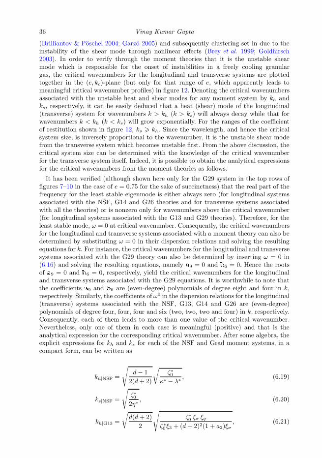
36 Vinay Kumar Gupta
(Brilliantov & Poschel 2004; Garzo 2005) and subsequently clustering set in due to theinstability of the shear mode through nonlinear effects (Brey et al. 1999; Goldhirsch2003). In order to verify through the moment theories that it is the unstable shearmode which is responsible for the onset of instabilities in a freely cooling granulargas, the critical wavenumbers for the longitudinal and transverse systems are plottedtogether in the (e, kc)-plane (but only for that range of e, which apparently leads tomeaningful critical wavenumber profiles) in figure 12. Denoting the critical wavenumbersassociated with the unstable heat and shear modes for any moment system by kh andks, respectively, it can be easily deduced that a heat (shear) mode of the longitudinal(transverse) system for wavenumbers k > kh (k > ks) will always decay while that forwavenumbers k < kh (k < ks) will grow exponentially. For the ranges of the coefficientof restitution shown in figure 12, ks > kh. Since the wavelength, and hence the criticalsystem size, is inversely proportional to the wavenumber, it is the unstable shear modefrom the transverse system which becomes unstable first. From the above discussion, thecritical system size can be determined with the knowledge of the critical wavenumberfor the transverse system itself. Indeed, it is possible to obtain the analytical expressionsfor the critical wavenumbers from the moment theories as follows.
It has been verified (although shown here only for the G29 system in the top rows offigures 7–10 in the case of e = 0.75 for the sake of succinctness) that the real part of thefrequency for the least stable eigenmode is either always zero (for longitudinal systemsassociated with the NSF, G14 and G26 theories and for transverse systems associatedwith all the theories) or is nonzero only for wavenumbers above the critical wavenumber(for longitudinal systems associated with the G13 and G29 theories). Therefore, for theleast stable mode, ω = 0 at critical wavenumber. Consequently, the critical wavenumbersfor the longitudinal and transverse systems associated with a moment theory can also bedetermined by substituting ω = 0 in their dispersion relations and solving the resultingequations for k. For instance, the critical wavenumbers for the longitudinal and transversesystems associated with the G29 theory can also be determined by inserting ω = 0 in(6.16) and solving the resulting equations, namely a9 = 0 and b6 = 0. Hence the rootsof a9 = 0 and b6 = 0, respectively, yield the critical wavenumbers for the longitudinaland transverse systems associated with the G29 equations. It is worthwhile to note thatthe coefficients a9 and b6 are (even-degree) polynomials of degree eight and four in k,respectively. Similarly, the coefficients of ω0 in the dispersion relations for the longitudinal(transverse) systems associated with the NSF, G13, G14 and G26 are (even-degree)polynomials of degree four, four, four and six (two, two, two and four) in k, respectively.Consequently, each of them leads to more than one value of the critical wavenumber.Nevertheless, only one of them in each case is meaningful (positive) and that is theanalytical expression for the corresponding critical wavenumber. After some algebra, theexplicit expressions for kh and ks for each of the NSF and Grad moment systems, in acompact form, can be written as
kh|NSF =
√
d− 1
2(d+ 2)
√
ζ∗0κ∗ − λ∗
, (6.19)
ks|NSF =
√
ζ∗02η∗
, (6.20)
kh|G13 =
√
d(d+ 2)
2
√
ζ∗0 ξσ ξqζ∗0 ξ3 + (d+ 2)2(1 + a2)ξσ
, (6.21)
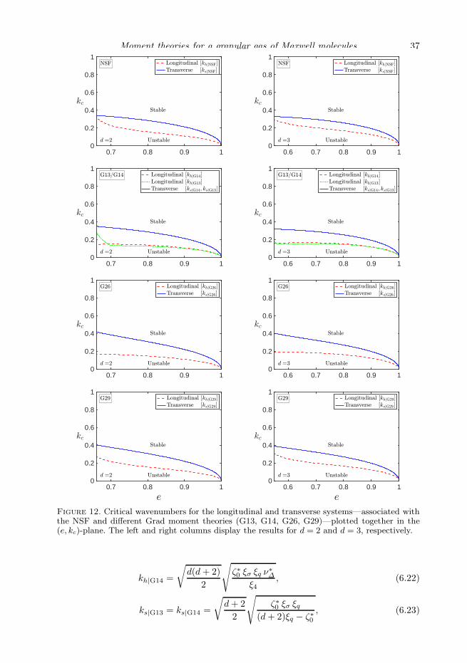
Moment theories for a granular gas of Maxwell molecules 37
0.7 0.8 0.9 10
0.2
0.4
0.6
0.8
1
0.6 0.7 0.8 0.9 10
0.2
0.4
0.6
0.8
1
0.7 0.8 0.9 10
0.2
0.4
0.6
0.8
1
0.6 0.7 0.8 0.9 10
0.2
0.4
0.6
0.8
1
0.7 0.8 0.9 10
0.2
0.4
0.6
0.8
1
0.6 0.7 0.8 0.9 10
0.2
0.4
0.6
0.8
1
0.7 0.8 0.9 10
0.2
0.4
0.6
0.8
1
0.6 0.7 0.8 0.9 10
0.2
0.4
0.6
0.8
1
Figure 12. Critical wavenumbers for the longitudinal and transverse systems—associated withthe NSF and different Grad moment theories (G13, G14, G26, G29)—plotted together in the(e, kc)-plane. The left and right columns display the results for d = 2 and d = 3, respectively.
kh|G14 =
√
d(d+ 2)
2
√
ζ∗0 ξσ ξq ν∗∆
ξ4, (6.22)
ks|G13 = ks|G14 =
√
d+ 2
2
√
ζ∗0 ξσ ξq(d+ 2)ξq − ζ∗0
, (6.23)
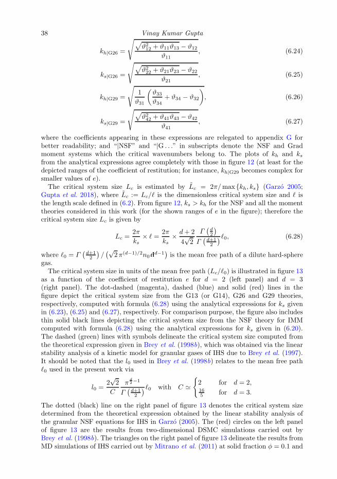
38 Vinay Kumar Gupta
kh|G26 =
√
√
ϑ212 + ϑ11ϑ13 − ϑ12ϑ11
, (6.24)
ks|G26 =
√
√
ϑ222 + ϑ21ϑ23 − ϑ22ϑ21
, (6.25)
kh|G29 =
√
1
ϑ31
(
ϑ33ϑ34
+ ϑ34 − ϑ32
)
, (6.26)
ks|G29 =
√
√
ϑ242 + ϑ41ϑ43 − ϑ42ϑ41
, (6.27)
where the coefficients appearing in these expressions are relegated to appendix G forbetter readability; and “|NSF” and “|G . . .” in subscripts denote the NSF and Gradmoment systems which the critical wavenumbers belong to. The plots of kh and ksfrom the analytical expressions agree completely with those in figure 12 (at least for thedepicted ranges of the coefficient of restitution; for instance, kh|G29 becomes complex forsmaller values of e).The critical system size Lc is estimated by Lc = 2π/maxkh, ks (Garzo 2005;
Gupta et al. 2018), where Lc := Lc/ℓ is the dimensionless critical system size and ℓ isthe length scale defined in (6.2). From figure 12, ks > kh for the NSF and all the momenttheories considered in this work (for the shown ranges of e in the figure); therefore thecritical system size Lc is given by
Lc =2π
ks× ℓ =
2π
ks× d+ 2
4√2
Γ(
d2
)
Γ(
d+12
)ℓ0, (6.28)
where ℓ0 = Γ(
d+12
)
/(√
2π(d−1)/2n0dd−1)
is the mean free path of a dilute hard-spheregas.The critical system size in units of the mean free path (Lc/ℓ0) is illustrated in figure 13
as a function of the coefficient of restitution e for d = 2 (left panel) and d = 3(right panel). The dot-dashed (magenta), dashed (blue) and solid (red) lines in thefigure depict the critical system size from the G13 (or G14), G26 and G29 theories,respectively, computed with formula (6.28) using the analytical expressions for ks givenin (6.23), (6.25) and (6.27), respectively. For comparison purpose, the figure also includesthin solid black lines depicting the critical system size from the NSF theory for IMMcomputed with formula (6.28) using the analytical expressions for ks given in (6.20).The dashed (green) lines with symbols delineate the critical system size computed fromthe theoretical expression given in Brey et al. (1998b), which was obtained via the linearstability analysis of a kinetic model for granular gases of IHS due to Brey et al. (1997).It should be noted that the l0 used in Brey et al. (1998b) relates to the mean free pathℓ0 used in the present work via
l0 =2√2
C
πd2−1
Γ(
d+12
)ℓ0 with C ≃
2 for d = 2,165 for d = 3.
The dotted (black) line on the right panel of figure 13 denotes the critical system sizedetermined from the theoretical expression obtained by the linear stability analysis ofthe granular NSF equations for IHS in Garzo (2005). The (red) circles on the left panelof figure 13 are the results from two-dimensional DSMC simulations carried out byBrey et al. (1998b). The triangles on the right panel of figure 13 delineate the results fromMD simulations of IHS carried out by Mitrano et al. (2011) at solid fraction φ = 0.1 and
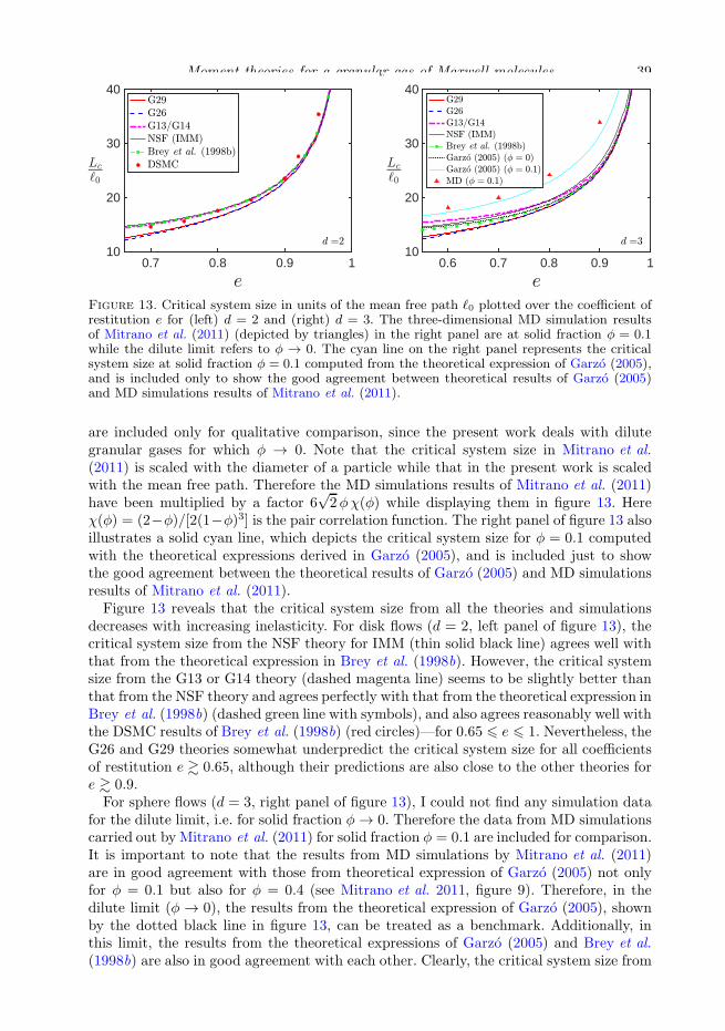
Moment theories for a granular gas of Maxwell molecules 39
0.7 0.8 0.9 110
20
30
40
0.6 0.7 0.8 0.9 110
20
30
40
Figure 13. Critical system size in units of the mean free path ℓ0 plotted over the coefficient ofrestitution e for (left) d = 2 and (right) d = 3. The three-dimensional MD simulation resultsof Mitrano et al. (2011) (depicted by triangles) in the right panel are at solid fraction φ = 0.1while the dilute limit refers to φ → 0. The cyan line on the right panel represents the criticalsystem size at solid fraction φ = 0.1 computed from the theoretical expression of Garzo (2005),and is included only to show the good agreement between theoretical results of Garzo (2005)and MD simulations results of Mitrano et al. (2011).
are included only for qualitative comparison, since the present work deals with dilutegranular gases for which φ → 0. Note that the critical system size in Mitrano et al.(2011) is scaled with the diameter of a particle while that in the present work is scaledwith the mean free path. Therefore the MD simulations results of Mitrano et al. (2011)have been multiplied by a factor 6
√2φχ(φ) while displaying them in figure 13. Here
χ(φ) = (2−φ)/[2(1−φ)3] is the pair correlation function. The right panel of figure 13 alsoillustrates a solid cyan line, which depicts the critical system size for φ = 0.1 computedwith the theoretical expressions derived in Garzo (2005), and is included just to showthe good agreement between the theoretical results of Garzo (2005) and MD simulationsresults of Mitrano et al. (2011).Figure 13 reveals that the critical system size from all the theories and simulations
decreases with increasing inelasticity. For disk flows (d = 2, left panel of figure 13), thecritical system size from the NSF theory for IMM (thin solid black line) agrees well withthat from the theoretical expression in Brey et al. (1998b). However, the critical systemsize from the G13 or G14 theory (dashed magenta line) seems to be slightly better thanthat from the NSF theory and agrees perfectly with that from the theoretical expression inBrey et al. (1998b) (dashed green line with symbols), and also agrees reasonably well withthe DSMC results of Brey et al. (1998b) (red circles)—for 0.65 6 e 6 1. Nevertheless, theG26 and G29 theories somewhat underpredict the critical system size for all coefficientsof restitution e & 0.65, although their predictions are also close to the other theories fore & 0.9.For sphere flows (d = 3, right panel of figure 13), I could not find any simulation data
for the dilute limit, i.e. for solid fraction φ→ 0. Therefore the data from MD simulationscarried out by Mitrano et al. (2011) for solid fraction φ = 0.1 are included for comparison.It is important to note that the results from MD simulations by Mitrano et al. (2011)are in good agreement with those from theoretical expression of Garzo (2005) not onlyfor φ = 0.1 but also for φ = 0.4 (see Mitrano et al. 2011, figure 9). Therefore, in thedilute limit (φ → 0), the results from the theoretical expression of Garzo (2005), shownby the dotted black line in figure 13, can be treated as a benchmark. Additionally, inthis limit, the results from the theoretical expressions of Garzo (2005) and Brey et al.(1998b) are also in good agreement with each other. Clearly, the critical system size from
40 Vinay Kumar Gupta
the NSF theory for IMM is again in reasonably good agreement with that from Garzo(2005). Moreover, the critical system sizes from all the moment theories are also in goodagreement with that from Garzo (2005) for e & 0.85, but deviate slightly from the resultsof Garzo (2005) for 0.55 . e . 0.85, where the G26 and G29 theories again underpredictthe critical system size while the G13 or G14 theory overpredicts it. Between the G26and G29 theories, the latter seems to perform slightly better at moderate values of thecoefficient of restitution for both d = 2 and d = 3.
From figure 13, it is apparent that the critical system size obtained from the NSF andGrad moment theories for IMM is in qualitatively good agreement with that obtainedfrom the NSF-level theories and simulations for IHD/IHS, although it is also noticeablefrom the figure that some lower-order Grad moment theories (e.g. the G13 or G14 theory)perform better than some higher-order Grad moment theories (e.g. the G26 theory).A possible reason for this could be the choice of the effective collision frequency ν inthe IMM model (see (2.3a)) that was chosen in such a way that the cooling rates forIHS and IMM remain exactly the same while the collisional production terms in theother moment equations for IMM follow accordingly based on this choice of the effectivecollision frequency. Consequently, with this choice of the effective collision frequency,even the NSF equations for IMM seem to perform better than some higher-order momentmodels. Therefore it would be interesting to explore other possible choices for the effectivecollision frequency in the future in such a way that the results from the Boltzmannequations for IHS and IMM agree in an optimal way so that a higher-order momentmodel would perform better than a lower-order moment model in the case of IMM,similarly to moment models for IHS.
7. Conclusion
Grad moment equations—consisting of up to 29 moments—for a d-dimensional dilutegranular gas composed of IMM have been derived from the Boltzmann equation forIMM via the Grad moment method. A strategy for computing the collisional productionterms associated with these moment equations in an automated way has been presented.Although the Maxwell interaction potential had been devised in such a way that theexplicit form of the distribution function is not required to be known for determiningthe collisional production terms, and therefore the collisional production terms for IMMcan, in principle, be evaluated using pen and paper, yet the complexity increases withan increase in the number of moments. Thus the presented strategy for computing thecollisional production terms associated with the moment equations would really be usefulwhen considering even more moments.
The transport coefficients in the NSF laws for dilute granular gases of IMM have beendetermined by following a procedure due to Garzo (2013) and it has been shown thatthe G13 equations for IMM are sufficient to derive the first-order (i.e. the NSF-level)transport coefficients and that the higher moments do not play any role in determiningthe NSF transport coefficients for IMM since the stress and heat flux balance equations atthis order do not have any dependence on the higher moments. The higher-order momentequations will be required only for computing the transport coefficients beyond the NSFlevel. However, since the present work already provides some higher-order Grad momentequations, it would be interesting to compute the transport coefficients beyond the NSFlevel in the future by relating the Grad moment equations to the Burnett equationsfor IMM. Although the Grad moment theories for IMM presented in this work seem tooverestimate all the transport coefficients, the NSF-level transport coefficients for IMM
Moment theories for a granular gas of Maxwell molecules 41
obtained with the Grad moment theories and with the CE expansion (Santos 2003) arein complete agreement.The HCS of a freely cooling granular gas has then been investigated and it has been
found that the decay of the granular temperature in the HCS obeys Haff’s law but, incontrast to the case of IHS, does not depend on the higher moments since the fourthcumulant does not enter the energy balance equation for IMM. Yet, Haff’s laws for IMMand IHS have been found to be in good agreement with each other. Furthermore, the otherhigher moments have been found to relax much faster than the granular temperature.
As an application of the derived moment models, a linear stability analysis hasbeen performed to scrutinise the stability of the HCS due to small perturbations. Bydecomposing each moment system into the longitudinal and transverse systems, it hasbeen shown that a heat mode from the longitudinal system and a shear mode from thetransverse system associated with each moment system are unstable for (moderatelyto nearly elastic) granular gases and that the unstable shear mode from the transversesystem initiates instability in a homogeneously cooling granular gas. To assess the linearstability results, the critical system size for the onset of instability is investigated, andit has been found that the Grad moment theories for IMM yield a reasonably goodestimate of the critical system size for granular gases with moderate to large coefficientsof restitution.It is important to note that the only assumption on the coefficient of restitution in this
work is that it is a constant. Therefore the present work should, in principle, be applicableto granular gases with any degree of inelasticity, which is not the case unfortunately.Nevertheless, this should not be thought of as a problem with moment models presentedhere, rather it is a problem with the IMM model itself; for instance, the IMM modelyields negative values for the coefficient of thermal conductivity below a certain value ofthe coefficient of restitution (Santos 2003; Garzo & Santos 2011).
It is anticipated that the Grad moment systems for dilute granular gases of IMM,similarly to those for monatomic gases, will also suffer from the loss of hyperbolicity.Therefore the hyperbolicity of these systems needs to be investigated in the future,which will also be useful in developing suitable numerical methods for solving them.Moreover, to overcome the undesirable consequences of the loss of hyperbolicity, aregularisation of Grad moment equations might also be necessary. The usefulness ofthe derived Grad moment systems is substantially limited by the unavailability ofboundary conditions. Hence the development of boundary conditions complementingthese Grad moment systems should be an immediate follow-up to the present work.Notwithstanding, the Grad moment systems presented in this work will be useful indescribing granular processes involving large spatial gradients and are expected to pavethe way to further developments including the developments of regularised momentmodels, required boundary conditions, efficient numerical frameworks including the MFS.
Acknowledgments
The author appreciates the anonymous referees for their informative suggestions, whichhave helped to improve the paper. The author gratefully acknowledges the financialsupports through the “MATRICS” project MTR/2017/000693 funded by the SERB,India and through the Commonwealth Rutherford Fellowship availed at the Universityof Warwick, UK. The author is thankful to Prof. Vicente Garzo and Prof. Andres Santosfor some helpful suggestions on this work during the RGD31 symposium in Glasgow, toDr. James Sprittles, Prof. Duncan Lockerby, Dr. Anirudh Singh Rana and Dr. Priyanka
42 Vinay Kumar Gupta
Shukla for some fruitful discussions, and to Prof. Manuel Torrilhon for implementing inMathematica the Einstein summation, which has been used in this work.
Declaration of interests
The author reports no conflict of interest.
Appendix A. Symmetric and traceless part of a tensor
Needless to say, the symmetric and traceless part of a tensor of rank zero or one is thattensor itself. The symmetric and traceless part of a rank two tensor Aij in d dimensionsis given by
A〈ij〉 = A(ij) −1
dAkkδij , (A 1)
where the round brackets around the indices in (A 1) and in what follows always denotethe symmetric part of the corresponding tensor. Here, A(ij) = (Aij + Aji)/2 is thesymmetric part of Aij .The symmetric and traceless part of a rank three tensor Aijk in d dimensions is given by
A〈ijk〉 = A(ijk) −1
d+ 2
[
A(ill)δjk +A(ljl)δik +A(llk)δij
]
, (A 2)
where A(ijk) = (Aijk +Aikj +Ajik +Ajki+Akji+Akij)/6 is the symmetric part of Aijk.The symmetric and traceless part of a rank four tensor Aijkl in d dimensions is given by
A〈ijkl〉 = A(ijkl) −1
d+ 4
[
A(ijss)δkl +A(isks)δjl +A(issl)δjk +A(sjks)δil +A(sjsl)δik
+A(sskl)δij
]
+1
(d+ 2)(d+ 4)A(rrss)
[
δijδkl + δikδjl + δilδjk
]
, (A 3)
where A(ijkl) = (Aijkl + Aijlk + Aikjl + Aiklj + Ailjk + Ailkj + Ajikl + Ajilk + Ajkil +Ajkli +Ajlik +Ajlki+Akijl +Akilj +Akjil +Akjli+Aklij +Aklji+Alijk +Alikj +Aljik +Aljki +Alkij +Alkji)/24 is the symmetric part of Aijkl.The symmetric and traceless part of a rank n tensor Ai1i2...in in d dimensions is given by
A〈i1i2...in〉 = A(i1i2...in) + βn,1
[
A(rri3i4...in)δi1i2 + all permutations]
+ βn,2
[
A(rrssi5i6...in)δi1i2δi3i4 + all permutations]
+ . . . , (A 4)
where the coefficients βn,k are given by
βn,k =(−1)k
k−1∏
j=0
(
d+ 2n− 2j − 4)
(A 5)
and the symmetric part of Ai1i2...in is given by
A(i1i2...in) =Ai1i2i3i4...in +Ai2i1i3i4...in + all permutations
n!. (A 6)
Appendix B. Computation of the collisional production terms
For an arbitrary function ψ(t,x, c), the collisional production term (or collisionalmoment) associated with it—on using the symmetry properties of the Boltzmann collision
Moment theories for a granular gas of Maxwell molecules 43
operator—reads (Garzo & Santos 2007)∫
ψ(c)J [c|f, f ] dc =ν
nΩd
∫∫∫
[
ψ(t,x, c′)− ψ(t,x, c)]
f(c)f(c1) dk dc dc1, (B 1)
where the velocity with single prime denotes the post-collisional velocity in a directcollision that transforms the pre-collision velocities c and c1 of the colliding molecules tothe post-collisional velocities c′ and c′1 via the relations (Brilliantov & Poschel 2004)
c′ = c− 1 + e
2(k · g)k and c′1 = c1 +
1 + e
2(k · g)k. (B 2a,b)
Typically, ψ is of the tensorial form: ψ = mC2aC〈i1Ci2 · · ·Cin〉 and hence the generalform of the collisional production term is
Pai1···in =
m ν
nΩd
∫∫[∫
(C′)2aC′
〈i1C′
i2 · · ·C′in〉
− C2aC〈i1Ci2 · · ·Cin〉
dk
]
× f(c)f(c1) dc dc1. (B 3)
However, since the squared velocities in (B 3) can be easily expressed in index notationusing the Einstein summation convention, for instance C2 = Ci0Ci0 , and the indices ineach term of (B 3) can be adjusted accordingly, it is convenient to first compute
Pi1···in =m ν
nΩd
∫∫[∫
(
C′i1C
′i2 · · ·C
′in − Ci1Ci2 · · ·Cin
)
dk
]
f(c)f(c1) dc dc1 (B 4)
instead of computing (B 3) directly.To compute the right-hand side of (B 4), the post-collisional peculiar velocities (marked
with primes) in (B 4) are replaced with the pre-collisional peculiar velocities by exploitingthe definition of the peculiar velocity and relation (B 2a). This changes the product ofthe post-collisional peculiar velocities in (B 4) to
C′i1C
′i2 · · ·C
′in =
n∑
j=0
(−w0)j
(
n
j
)
k(i1 ki2 · · · kijCij+1Cij+2
· · ·Cin−1Cin)(k · g)j , (B 5)
where w0 = (1 + e)/2 and the round brackets around the indices again denote the sym-metric part of the corresponding tensor (see appendix A for its definition). Substituting(B 5) into (B 4), one obtains
Pi1...in =m ν
nΩd
n∑
j=1
(−w0)j
(
n
j
)∫∫
gjI(i1...ijCij+1Cij+2
· · ·Cin−1Cin)f(c)f(c1) dc dc1,
(B 6)
where
Ii1i2...in =
∫
ki1 ki2 · · · kin(k · g)n dk (B 7)
is termed as the scattering vector integral with g = g/g. The structure of the integrandin (B 7) suggests that Ii1i2...in will have the form
Ii1i2...in =
⌊n2 ⌋∑
β=0
a(n)β δ(i1i2δi3i4 · · · δi2β−1i2β
gi2β+1
g
gi2β+2
g· · · gin)
g, (B 8)
where the unknown coefficients a(n)β depend only on the dimension d, and are computed
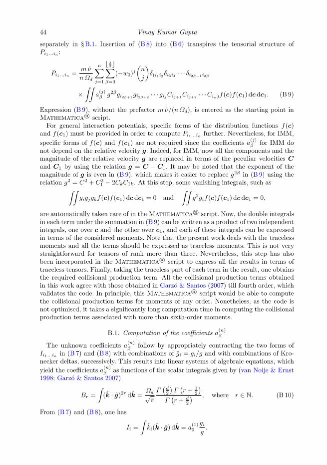
44 Vinay Kumar Gupta
separately in §B.1. Insertion of (B 8) into (B 6) transpires the tensorial structure ofPi1...in :
Pi1...in =m ν
nΩd
n∑
j=1
⌊ j2⌋∑
β=0
(−w0)j
(
n
j
)
δ(i1i2δi3i4 · · · δi2β−1i2β
×∫∫
a(j)β g2βgi2β+1
gi2β+2· · · gijCij+1
Cij+2· · ·Cin)f(c)f(c1) dc dc1. (B 9)
Expression (B 9), without the prefactor m ν/(nΩd), is entered as the starting point inMathematica® script.For general interaction potentials, specific forms of the distribution functions f(c)
and f(c1) must be provided in order to compute Pi1...in further. Nevertheless, for IMM,
specific forms of f(c) and f(c1) are not required since the coefficients a(j)β for IMM do
not depend on the relative velocity g. Indeed, for IMM, now all the components and themagnitude of the relative velocity g are replaced in terms of the peculiar velocities C
and C1 by using the relation g = C − C1. It may be noted that the exponent of themagnitude of g is even in (B 9), which makes it easier to replace g2β in (B 9) using therelation g2 = C2 + C2
1 − 2CkC1k. At this step, some vanishing integrals, such as∫∫
gigjgkf(c)f(c1) dc dc1 = 0 and
∫∫
g2gif(c)f(c1) dc dc1 = 0,
are automatically taken care of in the Mathematica® script. Now, the double integralsin each term under the summation in (B 9) can be written as a product of two independentintegrals, one over c and the other over c1, and each of these integrals can be expressedin terms of the considered moments. Note that the present work deals with the tracelessmoments and all the terms should be expressed as traceless moments. This is not verystraightforward for tensors of rank more than three. Nevertheless, this step has alsobeen incorporated in the Mathematica® script to express all the results in terms oftraceless tensors. Finally, taking the traceless part of each term in the result, one obtainsthe required collisional production term. All the collisional production terms obtainedin this work agree with those obtained in Garzo & Santos (2007) till fourth order, whichvalidates the code. In principle, this Mathematica® script would be able to computethe collisional production terms for moments of any order. Nonetheless, as the code isnot optimised, it takes a significantly long computation time in computing the collisionalproduction terms associated with more than sixth-order moments.
B.1. Computation of the coefficients a(n)β
The unknown coefficients a(n)β follow by appropriately contracting the two forms of
Ii1...in in (B 7) and (B 8) with combinations of gi = gi/g and with combinations of Kro-necker deltas, successively. This results into linear systems of algebraic equations, which
yield the coefficients a(n)β as functions of the scalar integrals given by (van Noije & Ernst
1998; Garzo & Santos 2007)
Br =
∫
(k · g)2r dk =Ωd√π
Γ(
d2
)
Γ(
r + 12
)
Γ(
r + d2
) , where r ∈ N. (B 10)
From (B7) and (B 8), one has
Ii =
∫
ki(k · g) dk = a(1)0
gig.
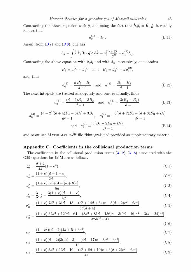
Moment theories for a granular gas of Maxwell molecules 45
Contracting the above equation with gi and using the fact that kigi = k · g, it readilyfollows that
a(1)0 = B1. (B 11)
Again, from (B 7) and (B 8), one has
Iij =
∫
kikj(k · g)2 dk = a(2)0
gigjg 2
+ a(2)1 δij .
Contracting the above equation with gigj and with δij successively, one obtains
B2 = a(2)0 + a
(2)1 and B1 = a
(2)0 + d a
(2)1 ,
and, thus
a(2)0 =
dB2 −B1
d− 1and a
(2)1 =
B1 −B2
d− 1. (B 12)
The next integrals are treated analogously and one, eventually, finds
a(3)0 =
(d+ 2)B3 − 3B2
d− 1and a
(3)1 =
3(B2 −B3)
d− 1, (B 13)
a(4)0 =
(d+ 2)[(d+ 4)B4 − 6B3] + 3B2
d2 − 1, a
(4)1 = −6[(d+ 2)B4 − (d+ 3)B3 +B2]
d2 − 1
and a(4)2 =
3(B4 − 2B3 +B2)
d2 − 1, (B 14)
and so on; see Mathematica® file “kintegrals.nb” provided as supplementary material.
Appendix C. Coefficients in the collisional production terms
The coefficients in the collisional production terms (3.12)–(3.18) associated with theG29 equations for IMM are as follows.
ζ∗0 =d+ 2
4d(1− e2), (C 1)
ν∗σ =(1 + e)(d+ 1− e)
2d, (C 2)
ν∗q =(1 + e)[5d+ 4− (d+ 8)e]
8d, (C 3)
ν∗m =3
2ν∗σ =
3(1 + e)(d+ 1− e)
4d, (C 4)
ν∗R =(1 + e)[7d2 + 31d+ 18− (d2 + 14d+ 34)e+ 3(d+ 2)e2 − 6e3]
8d(d+ 4), (C 5)
ν∗ϕ =(1 + e)[32d2 + 129d+ 64− (8d2 + 81d+ 136)e+ 3(9d+ 16)e2 − 3(d+ 24)e3]
32d(d+ 4),
(C 6)
α0 =(1− e2)(d+ 2)(4d+ 5 + 3e2)
8, (C 7)
α1 =(1 + e)(d+ 2)[3(4d+ 3)− (4d+ 17)e+ 3e2 − 3e3]
16, (C 8)
α2 =(1 + e)[3d2 + 13d+ 10− (d2 + 8d+ 10)e+ 3(d+ 2)e2 − 6e3]
4d, (C 9)
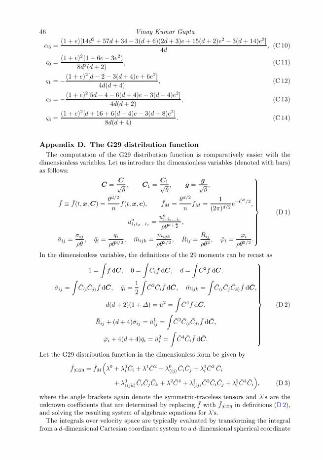
46 Vinay Kumar Gupta
α3 =(1 + e)[14d2 + 57d+ 34− 3(d+ 6)(2d+ 3)e+ 15(d+ 2)e2 − 3(d+ 14)e3]
4d, (C 10)
ς0 =(1 + e)2(1 + 6e− 3e2)
8d2(d+ 2), (C 11)
ς1 = − (1 + e)2[d− 2− 3(d+ 4)e+ 6e2]
4d(d+ 4), (C 12)
ς2 = − (1 + e)2[5d− 4− 6(d+ 4)e− 3(d− 4)e2]
4d(d+ 2), (C 13)
ς3 =(1 + e)2[d+ 16 + 6(d+ 4)e− 3(d+ 8)e2]
8d(d+ 4). (C 14)
Appendix D. The G29 distribution function
The computation of the G29 distribution function is comparatively easier with thedimensionless variables. Let us introduce the dimensionless variables (denoted with bars)as follows:
C =C√θ, C1 =
C1√θ, g =
g√θ,
f ≡ f(t,x,C) =θd/2
nf(t,x, c), fM =
θd/2
nfM =
1
(2π)d/2e−C2/2,
uai1i2...ir =uai1i2...irρθa+
r2
,
σij =σijρθ, qi =
qiρθ3/2
, mijk =mijk
ρθ3/2, Rij =
Rij
ρθ2, ϕi =
ϕi
ρθ5/2.
(D 1)
In the dimensionless variables, the definitions of the 29 moments can be recast as
1 =
∫
f dC, 0 =
∫
Cif dC, d =
∫
C2f dC,
σij =
∫
C〈iCj〉f dC, qi =1
2
∫
C2Cif dC, mijk =
∫
C〈iCjCk〉f dC,
d(d + 2)(1 +∆) = u2 =
∫
C4f dC,
Rij + (d+ 4)σij = u1ij =
∫
C2C〈iCj〉f dC,
ϕi + 4(d+ 4)qi = u2i =
∫
C4Cif dC.
(D 2)
Let the G29 distribution function in the dimensionless form be given by
f|G29 = fM
(
λ0 + λ0i Ci + λ1C2 + λ0〈ij〉CiCj + λ1i C2 Ci
+ λ0〈ijk〉CiCjCk + λ2C4 + λ1〈ij〉C2CiCj + λ2i C
4Ci
)
, (D 3)
where the angle brackets again denote the symmetric-traceless tensors and λ’s are theunknown coefficients that are determined by replacing f with f|G29 in definitions (D 2),and solving the resulting system of algebraic equations for λ’s.The integrals over velocity space are typically evaluated by transforming the integral
from a d-dimensional Cartesian coordinate system to a d-dimensional spherical coordinate
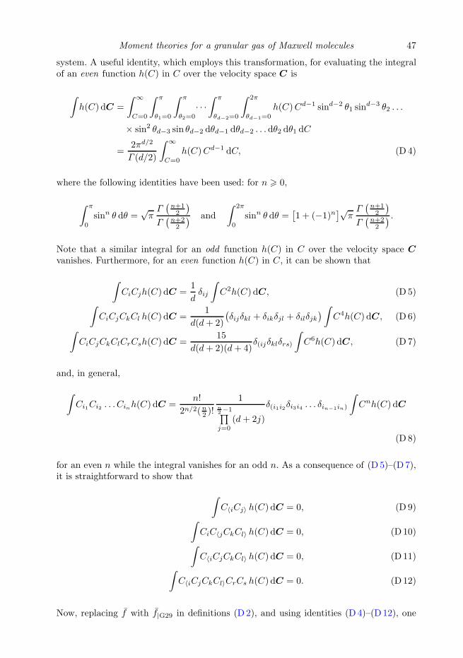
Moment theories for a granular gas of Maxwell molecules 47
system. A useful identity, which employs this transformation, for evaluating the integralof an even function h(C) in C over the velocity space C is
∫
h(C) dC =
∫ ∞
C=0
∫ π
θ1=0
∫ π
θ2=0
· · ·∫ π
θd−2=0
∫ 2π
θd−1=0
h(C)Cd−1 sind−2 θ1 sind−3 θ2 . . .
× sin2 θd−3 sin θd−2 dθd−1 dθd−2 . . . dθ2 dθ1 dC
=2πd/2
Γ (d/2)
∫ ∞
C=0
h(C)Cd−1 dC, (D 4)
where the following identities have been used: for n > 0,
∫ π
0
sinn θ dθ =√πΓ(
n+12
)
Γ(
n+22
) and
∫ 2π
0
sinn θ dθ =[
1 + (−1)n]√πΓ(
n+12
)
Γ(
n+22
) .
Note that a similar integral for an odd function h(C) in C over the velocity space C
vanishes. Furthermore, for an even function h(C) in C, it can be shown that
∫
CiCjh(C) dC =1
dδij
∫
C2h(C) dC, (D 5)
∫
CiCjCkCl h(C) dC =1
d(d+ 2)
(
δijδkl + δikδjl + δilδjk)
∫
C4h(C) dC, (D 6)
∫
CiCjCkClCrCsh(C) dC =15
d(d+ 2)(d+ 4)δ(ijδklδrs)
∫
C6h(C) dC, (D 7)
and, in general,
∫
Ci1Ci2 . . . Cinh(C) dC =n!
2n/2(n2 )!
1n2−1∏
j=0
(d+ 2j)
δ(i1i2δi3i4 . . . δin−1in)
∫
Cnh(C) dC
(D 8)
for an even n while the integral vanishes for an odd n. As a consequence of (D 5)–(D7),it is straightforward to show that
∫
C〈iCj〉 h(C) dC = 0, (D 9)
∫
CiC〈jCkCl〉 h(C) dC = 0, (D 10)
∫
C〈iCjCkCl〉 h(C) dC = 0, (D 11)
∫
C〈iCjCkCl〉CrCs h(C) dC = 0. (D 12)
Now, replacing f with f|G29 in definitions (D 2), and using identities (D 4)–(D12), one
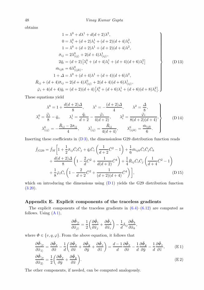
48 Vinay Kumar Gupta
obtains
1 = λ0 + dλ1 + d(d+ 2)λ2,
0 = λ0i + (d+ 2)λ1i + (d+ 2)(d+ 4)λ2i ,
1 = λ0 + (d+ 2)λ1 + (d+ 2)(d+ 4)λ2,
σij = 2λ0〈ij〉 + 2(d+ 4)λ1〈ij〉,
2qi = (d+ 2)[
λ0i + (d+ 4)λ1i + (d+ 4)(d+ 6)λ2i]
mijk = 6λ0〈ijk〉,
1 +∆ = λ0 + (d+ 4)λ1 + (d+ 4)(d+ 6)λ2,
Rij + (d+ 4)σij = 2(d+ 4)λ0〈ij〉 + 2(d+ 4)(d+ 6)λ1〈ij〉,
ϕi + 4(d+ 4)qi = (d+ 2)(d+ 4)[
λ0i + (d+ 6)λ1i + (d+ 6)(d+ 8)λ2i]
.
(D 13)
These equations yield
λ0 = 1 +d(d + 2)∆
8, λ1 = − (d+ 2)∆
4, λ2 =
∆
8,
λ0i =ϕi
8− qi, λ1i =
qid+ 2
− ϕi
4(d+ 2), λ2i =
ϕi
8(d+ 2)(d+ 4),
λ0〈ij〉 = − Rij − 2σij4
, λ1〈ij〉 =Rij
4(d+ 4), λ0〈ijk〉 =
mijk
6.
(D 14)
Inserting these coefficients in (D 3), the dimensionless G29 distribution function reads
f|G29 = fM
[
1 +1
2σijCiCj + qiCi
(
1
d+ 2C2 − 1
)
+1
6mijkCiCjCk
+d(d+ 2)∆
8
(
1− 2
dC2 +
1
d(d+ 2)C4
)
+1
4RijCiCj
(
1
d+ 4C2 − 1
)
+1
8ϕiCi
(
1− 2
d+ 2C2 +
1
(d+ 2)(d+ 4)C4
)]
, (D 15)
which on introducing the dimensions using (D 1) yields the G29 distribution function(3.20).
Appendix E. Explicit components of the traceless gradients
The explicit components of the traceless gradients in (6.4)–(6.12) are computed asfollows. Using (A 1),
∂Φ〈i
∂xj〉=
1
2
(
∂Φi
∂xj+∂Φj
∂xi
)
− 1
dδij∂Φk
∂xk,
where Φ ∈ v, q, ϕ. From the above equation, it follows that
∂Φ〈x
∂x1〉=∂Φx
∂x− 1
d
(
∂Φx
∂x+∂Φy
∂y+∂Φz
∂z
)
=d− 1
d
∂Φx
∂x− 1
d
∂Φy
∂y− 1
d
∂Φz
∂z, (E 1)
∂Φ〈x
∂x2〉=
1
2
(
∂Φx
∂y+∂Φy
∂x
)
. (E 2)
The other components, if needed, can be computed analogously.
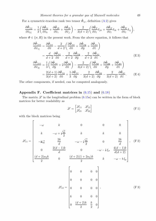
Moment theories for a granular gas of Maxwell molecules 49
For a symmetric-traceless rank two tensor Φij , definition (A 2) gives
∂Φ〈ij
∂xk〉=
1
3
(
∂Φij
∂xk+∂Φjk
∂xi+∂Φik
∂xj
)
− 2
3(d+ 2)
(
∂Φil
∂xlδjk +
∂Φjl
∂xlδik +
∂Φkl
∂xlδij
)
,
where Φ ∈ σ,R in the present work. From the above equation, it follows that
∂Φ〈xx
∂x1〉=∂Φxx
∂x− 2
d+ 2
(
∂Φxx
∂x+∂Φxy
∂y+∂Φxz
∂z
)
=d
d+ 2
∂Φxx
∂x− 2
d+ 2
∂Φxy
∂y− 2
d+ 2
∂Φxz
∂z, (E 3)
∂Φ〈xx
∂x2〉=
1
3
(
∂Φxx
∂y+ 2
∂Φxy
∂x
)
− 2
3(d+ 2)
(
∂Φxy
∂x+∂Φyy
∂y+∂Φyz
∂z
)
=2(d+ 1)
3(d+ 2)
∂Φxy
∂x+
1
3
∂Φxx
∂y− 2
3(d+ 2)
∂Φyy
∂y− 2
3(d+ 2)
∂Φyz
∂z. (E 4)
The other components, if needed, can be computed analogously.
Appendix F. Coefficient matrices in (6.15) and (6.18)
The matrix L in the longitudinal problem (6.15a) can be written in the form of blockmatrices for better readability as
L =
[
L11 L12
L21 L22
]
(F 1)
with the block matrices being
L11 =
−ω k 0 0 0
k −ω + i
ζ∗02
k k 0
−iζ∗02k
d−ω − i
ζ∗02
02k
d
02(d− 1)k
d0 −ω − i ξσ
4(d− 1)k
d(d+ 2)
(d+ 2)a2k
20
(d+ 2)(1 + 2a2)k
2k −ω − i ξq
, (F 2)
L12 =
0 0 0 0
0 0 0 0
0 0 0 0
k 0 0 0
0(d+ 2)k
2
k
20
, (F 3)
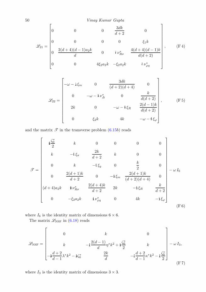
50 Vinay Kumar Gupta
L21 =
0 0 03dk
d+ 20
0 0 0 0 ξ1k
02(d+ 4)(d− 1)a2k
d0 i ν∗Rσ
4(d+ 4)(d− 1)k
d(d+ 2)
0 0 4ξ2a2k −ξ2a2k i ν∗ϕq
, (F 4)
L22 =
−ω − i ξm 03dk
(d+ 2)(d+ 4)0
0 −ω − i ν∗∆ 0k
d(d+ 2)
2k 0 −ω − i ξR2(d− 1)k
d(d+ 2)
0 ξ2k 4k −ω − i ξϕ
, (F 5)
and the matrix T in the transverse problem (6.15b) reads
T =
i
ζ∗02
k 0 0 0 0
k −i ξσ2k
d+ 2k 0 0
0 k −i ξq 0k
20
02(d+ 1)k
d+ 20 −i ξm
2(d+ 1)k
(d+ 2)(d+ 4)0
(d+ 4)a2k i ν∗Rσ
2(d+ 4)k
d+ 22k −i ξR
k
d+ 2
0 −ξ2a2k i ν∗ϕq 0 4k −i ξϕ
− ω I6
(F 6)
where I6 is the identity matrix of dimensions 6× 6.
The matrix LNSF in (6.18) reads
LNSF =
0 k 0
k −i2(d− 1)
dη∗k2 + i
ζ∗02
k
−id+ 2
d− 1λ∗k2 − iζ∗0
2k
d−id+ 2
d− 1κ∗k2 − i
ζ∗02
− ω I3,
(F 7)
where I3 is the identity matrix of dimensions 3× 3.
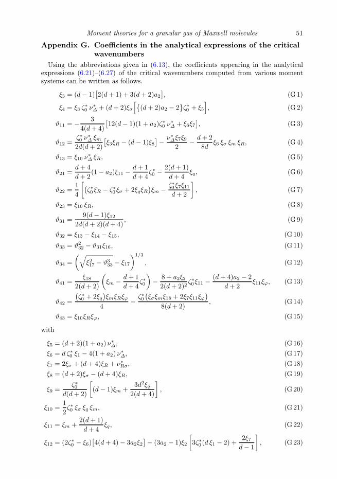
Moment theories for a granular gas of Maxwell molecules 51
Appendix G. Coefficients in the analytical expressions of the critical
wavenumbers
Using the abbreviations given in (6.13), the coefficients appearing in the analyticalexpressions (6.21)–(6.27) of the critical wavenumbers computed from various momentsystems can be written as follows.
ξ3 = (d− 1)[
2(d+ 1) + 3(d+ 2)a2]
, (G 1)
ξ4 = ξ3 ζ∗0 ν
∗∆ + (d+ 2)ξσ
[
(d+ 2)a2 − 2
ζ∗0 + ξ5
]
, (G 2)
ϑ11 = − 3
4(d+ 4)
[
12(d− 1)(1 + a2)ζ∗0 ν
∗∆ + ξ6ξ7
]
, (G 3)
ϑ12 =ζ∗0 ν
∗∆ ξm
2d(d+ 2)
[
ξ3ξR − (d− 1)ξ8]
− ν∗∆ξ7ξ92
− d+ 2
8dξ6 ξσ ξm ξR, (G 4)
ϑ13 = ξ10 ν∗∆ ξR, (G 5)
ϑ21 =d+ 4
d+ 2(1− a2)ξ11 −
d+ 1
d+ 4ζ∗0 − 2(d+ 1)
d+ 4ξq, (G 6)
ϑ22 =1
4
[
(
ζ∗0 ξR − ζ∗0 ξσ + 2ξqξR)
ξm − ζ∗0 ξ7ξ11d+ 2
]
, (G 7)
ϑ23 = ξ10 ξR, (G 8)
ϑ31 =9(d− 1)ξ12
2d(d+ 2)(d+ 4), (G 9)
ϑ32 = ξ13 − ξ14 − ξ15, (G 10)
ϑ33 = ϑ232 − ϑ31ξ16, (G 11)
ϑ34 =
(
√
ξ217 − ϑ333 − ξ17
)1/3
, (G 12)
ϑ41 =ξ18
2(d+ 2)
(
ξm − d+ 1
d+ 4ζ∗0
)
− 8 + a2ξ22(d+ 2)2
ζ∗0 ξ11 −(d+ 4)a2 − 2
d+ 2ξ11ξϕ, (G 13)
ϑ42 =
(
ζ∗0 + 2ξq)
ξmξRξϕ
4− ζ∗0
(
ξσξmξ18 + 2ξ7ξ11ξϕ)
8(d+ 2), (G 14)
ϑ43 = ξ10ξRξϕ, (G 15)
with
ξ5 = (d+ 2)(1 + a2) ν∗∆, (G 16)
ξ6 = d ζ∗0 ξ1 − 4(1 + a2) ν∗∆, (G 17)
ξ7 = 2ξσ + (d+ 4)ξR + ν∗Rσ, (G 18)
ξ8 = (d+ 2)ξσ − (d+ 4)ξR, (G 19)
ξ9 =ζ∗0
d(d+ 2)
[
(d− 1)ξm +3d2ξq
2(d+ 4)
]
, (G 20)
ξ10 =1
2ζ∗0 ξσ ξq ξm, (G 21)
ξ11 = ξm +2(d+ 1)
d+ 4ξq, (G 22)
ξ12 = (2ζ∗0 − ξ6)[
4(d+ 4)− 3a2ξ2]
− (3a2 − 1)ξ2
[
3ζ∗0 (d ξ1 − 2) +2ξ7d− 1
]
, (G 23)
52 Vinay Kumar Gupta
ξ13 =8(d− 1)
d2(d+ 2)ξσξm
(
ξ5 − a2ξ2 ν∗∆
)
+2 ξ9 ν
∗∆
d(d + 2)
[
4ξ3 − 9(d− 1)a2ξ2]
− 1
d(3a2 − 1)ξ2ξ19,
(G 24)
ξ14 =(d− 1)ζ∗0 ξmd2(d+ 2)
(
ξ2ξσ − 3a2ξ2ξR − 4ξ8)
+1
d
(
4− ξ2d+ 2
)[
d− 1
2ζ∗0 ξ1ξσξm − ξ7ξ9
]
,
(G 25)
ξ15 =3
4(d+ 4)
[
ζ∗0 ξ7ξ18d+ 2
+ (d ξ1 − 2)ζ∗0 ξ7ξϕ + (1 + a2)ν∗∆
6(d− 1)
d+ 2ζ∗0 ξ18 − 4ξ7ξϕ
]
,
(G 26)
ξ16 = (ξ5ξ19 − ξ7ξ9ν∗∆)ξϕ − 1
4ζ∗0 ξσξmξR
[
(d+ 2)ξ1ξϕ +ν∗ϕq
d
]
− ξ20, (G 27)
ξ17 = ϑ332 −3
2ϑ31(
ϑ32ξ16 + ξ10ν∗∆ξRξϕϑ31
)
, (G 28)
ξ18 = 8ξq + 2(d+ 2)ξϕ + ν∗ϕq, (G 29)
ξ19 =1
d
[
ξσ +3(d− 1)
d+ 2ζ∗0
]
ξmξR, (G 30)
ξ20 =1
2d(d+ 2)
[
2ξ2ξ10ξR + (d− 1)ζ∗0 ξ18ξσξmν∗∆
]
. (G 31)
REFERENCES
Alam, M., Chikkadi, V. & Gupta, V. K. 2009 Density waves and the effect of wall roughnessin granular Poiseuille flow: Simulation and linear stability. Eur. Phys. J. ST 179, 69–90.
Ben-Naim, E. & Krapivsky, P. L. 2000 Multiscaling in inelastic collisions. Phys. Rev. E61, R5–R8.
Ben-Naim, E. & Krapivsky, P. L. 2002 Scaling, multiscaling, and nontrivial exponents ininelastic collision processes. Phys. Rev. E 66, 011309.
Bisi, M., Spiga, G. & Toscani, G. 2004 Grad’s equations and hydrodynamics for weaklyinelastic granular flows. Phys. Fluids 16, 4235–4247.
Bobylev, A. V. 1982 The Chapman-Enskog and Grad methods for solving the Boltzmannequation. Sov. Phys. Dokl. 27, 29–31.
Brey, J. J., Dufty, J. W., Kim, C. S. & Santos, A. 1998a Hydrodynamics for granular flowat low density. Phys. Rev. E 58, 4638–4653.
Brey, J. J., Dufty, J. W. & Santos, A. 1997 Dissipative dynamics for hard spheres.J. Stat. Phys. 87, 1051–1066.
Brey, J. J., Garcıa de Soria, M. I. & Maynar, P. 2010 Breakdown of hydrodynamics inthe inelastic Maxwell model of granular gases. Phys. Rev. E 82, 021303.
Brey, J. J. & Ruiz-Montero, M. J. 2004 Simulation study of the Green-Kubo relations fordilute granular gases. Phys. Rev. E 70, 051301.
Brey, J. J., Ruiz-Montero, M. J. & Cubero, D. 1999 Origin of density clustering in a freelyevolving granular gas. Phys. Rev. E 60, 3150–3157.
Brey, J. J., Ruiz-Montero, M. J., Maynar, P. & Garcıa de Soria, M. I. 2005Hydrodynamic modes, Green–Kubo relations, and velocity correlations in dilute granulargases. J. Phys.: Condens. Matter 17, S2489–S2502.
Brey, J. J., Ruiz-Montero, M. J. & Moreno, F. 1998b Instability and spatial correlationsin a dilute granular gas. Phys. Fluids 10, 2976–2982.
Brilliantov, N. V., Formella, A. & Poschel, T. 2018 Increasing temperature of coolinggranular gases. Nat. Commun. 9, 797.
Brilliantov, N. V. & Poschel, T. 2004 Kinetic Theory of Granular Gases. New York: OxfordUniversity Press.
Moment theories for a granular gas of Maxwell molecules 53
Cai, Z., Fan, Y. & Li, R. 2013 Globally hyperbolic regularization of Grad’s moment systemin one-dimensional space. Comm. Math. Sci. 11, 547–571.
Cai, Z., Fan, Y. & Li, R. 2014a Globally hyperbolic regularization of Grad’s moment system.Comm. Pure Appl. Math. 67, 464–518.
Cai, Z., Fan, Y. & Li, R. 2014b On hyperbolicity of 13-moment system. Kinet. Relat. Models7, 415–432.
Cai, Z. & Li, R. 2010 Numerical regularized moment method of arbitrary order for Boltzmann-BGK equation. SIAM J. Sci. Comput. 32, 2875–2907.
Campbell, C. S. 1990 Rapid granular flows. Annu. Rev. Fluid Mech. 22, 57–90.
Carrillo, J. A., Cercignani, C. & Gamba, I. M. 2000 Steady states of a Boltzmann equationfor driven granular media. Phys. Rev. E 62, 7700–7707.
Chapman, S. & Cowling, T. G. 1970 The Mathematical Theory of Non-Uniform Gases.Cambridge, UK: Cambridge University Press.
Claydon, R., Shrestha, A., Rana, A. S., Sprittles, J. E. & Lockerby, D. A. 2017Fundamental solutions to the regularised 13-moment equations: efficient computation ofthree-dimensional kinetic effects. J. Fluid Mech. 833, R4.
Ernst, M. H. & Brito, R. 2002 Scaling solutions of inelastic Boltzmann equations with over-populated high energy tails. J. Stat. Phys. 109, 407–432.
Fan, Y., Koellermeier, J., Li, J., Li, R. & Torrilhon, M. 2016 Model reduction of kineticequations by operator projection. J. Stat. Phys. 162, 457–486.
Garzo, V. 2005 Instabilities in a free granular fluid described by the Enskog equation.Phys. Rev. E 72, 021106.
Garzo, V. 2013 Grad’s moment method for a granular fluid at moderate densities: Navier-Stokes transport coefficients. Phys. Fluids 25, 043301.
Garzo, V. 2019 Granular Gaseous Flows. Switzerland: Springer Nature.
Garzo, V. & Dufty, J. W. 1999 Dense fluid transport for inelastic hard spheres. Phys. Rev. E59, 5895–5911.
Garzo, V. & Santos, A. 2003 Kinetic Theory of Gases in Shear Flows. Nonlinear Transport .Dordrecht: Kluwer Academic Publishers.
Garzo, V. & Santos, A. 2007 Third and fourth degree collisional moments for inelasticMaxwell models. J. Phys. A: Math. Theor. 40, 14927–14943.
Garzo, V. & Santos, A. 2011 Hydrodynamics of inelastic Maxwell models.Math. Model. Nat. Phenom. 6, 37–76.
Garzo, V., Santos, A. & Montanero, J. M. 2007 Modified Sonine approximation for theNavier–Stokes transport coefficients of a granular gas. Physica A 376, 94–107.
Goldhirsch, I. 2003 Rapid granular flows. Annu. Rev. Fluid Mech. 35, 267–293.
Goldshtein, A. & Shapiro, M. 1995 Mechanics of collisional motion of granular materials.part 1. General hydrodynamic equations. J. Fluid Mech. 282, 75–114.
Grad, H. 1949 On the kinetic theory of rarefied gases. Comm. Pure Appl. Math. 2, 331–407.
Gu, X.-J. & Emerson, D. R. 2007 A computational strategy for the regularized 13 momentequations with enhanced wall-boundary conditions. J. Comput. Phys. 225, 263–283.
Gu, X.-J. & Emerson, D. R. 2009 A high-order moment approach for capturing non-equilibrium phenomena in the transition regime. J. Fluid Mech. 636, 177–216.
Gupta, V. K. 2011 Kinetic theory and Burnett order constitutive relations for a smooth granulargas. Master’s thesis, JNCASR, Bangalore, India.
Gupta, V. K. 2015 Mathematical modeling of rarefied gas mixtures. PhD thesis, RWTH AachenUniversity, Germany.
Gupta, V. K. & Shukla, P. 2017 Grad-type fourteen-moment theory for dilute granular gases.Indian Acad. Sci. Conf. Ser. 1, 133–143.
Gupta, V. K., Shukla, P. & Torrilhon, M. 2018 Higher-order moment theories for dilutegranular gases of smooth hard spheres. J. Fluid Mech. 836, 451–501.
Gupta, V. K., Struchtrup, H. & Torrilhon, M. 2016 Regularized moment equations forbinary gas mixtures: Derivation and linear analysis. Phys. Fluids 28, 042003.
Gupta, V. K. & Torrilhon, M. 2012 Automated Boltzmann collision integrals for momentequations. AIP Conf. Proc. 1501, 67–74.
54 Vinay Kumar Gupta
Gupta, V. K. & Torrilhon, M. 2015 Higher order moment equations for rarefied gas mixtures.Proc. Roy. Soc. A 471, 20140754.
Haff, P. K. 1983 Grain flow as a fluid-mechanical phenomenon. J. Fluid Mech. 134, 401–430.Jenkins, J. T. & Richman, M. W. 1985a Grad’s 13-moment system for a dense gas of inelastic
spheres. Arch. Ration. Mech. Anal. 87, 355–377.Jenkins, J. T. & Richman, M. W. 1985b Kinetic theory for plane flows of a dense gas of
identical, rough, inelastic, circular disks. Phys. Fluids 28, 3485–3494.Jenkins, J. T. & Savage, S. B. 1983 A theory for the rapid flow of identical, smooth, nearly
elastic, spherical particles. J. Fluid Mech. 130, 187–202.Junk, M. 1998 Domain of definition of Levermore’s five-moment system. J. Stat. Phys.
93, 1143–1167.Junk, M. & Unterreiter, A. 2002 Maximum entropy moment systems and Galilean
invariance. Continuum Mech. Thermodyn. 14, 563–576.Khalil, N., Garzo, V. & Santos, A. 2014 Hydrodynamic Burnett equations for inelastic
Maxwell models of granular gases. Phys. Rev. E 89, 052201.Koellermeier, J., Schaerer, R. P. & Torrilhon, M. 2014 A framework for hyperbolic
approximation of kinetic equations using quadrature-based projection methods.Kinet. Relat. Models 7, 531–549.
Koellermeier, J. & Torrilhon, M. 2017 Numerical study of partially conservative momentequations in kinetic theory. Commun. Comput. Phys. 21, 981–1011.
Koellermeier, J. & Torrilhon, M. 2018 Two-dimensional simulation of rarefied gas flowsusing quadrature-based moment equations. Multiscale Model. Simul. 16, 1059–1084.
Kohlstedt, K., Snezhko, A., Sapozhnikov, M. V., Aranson, I. S., Olafsen, J. S. &Ben-Naim, E. 2005 Velocity distributions of granular gases with drag and with long-range interactions. Phys. Rev. Lett. 95, 068001.
Kremer, G. M. 2010 An Introduction to the Boltzmann Equation and Transport Processes inGases. Berlin: Springer.
Kremer, G. M. & Marques Jr., W. 2011 Fourteen moment theory for granular gases.Kinet. Relat. Models 4, 317–331.
Kremer, G. M., Santos, A. & Garzo, V. 2014 Transport coefficients of a granular gas ofinelastic rough hard spheres. Phys. Rev. E 90, 022205.
Lasanta, A., Vega Reyes, F., Prados, A. & Santos, A. 2017 When the hotter cools morequickly: Mpemba effect in granular fluids. Phys. Rev. Lett. 119, 148001.
Levermore, C. D. 1996 Moment closure hierarchies for kinetic theories. J. Stat. Phys.83, 1021–1065.
Lockerby, D. A. & Collyer, B. 2016 Fundamental solutions to moment equations for thesimulation of microscale gas flows. J. Fluid Mech. 806, 413–436.
Lun, C. K. K., Savage, S. B., Jeffrey, D. J. & Chepurniy, N. 1984 Kinetic theories forgranular flow: inelastic particles in Couette flow and slightly inelastic particles in a generalflowfield. J. Fluid Mech. 140, 223–256.
Lutsko, J. F. 2005 Transport properties of dense dissipative hard-sphere fluids for arbitraryenergy loss models. Phys. Rev. E 72, 021306.
Maxwell, J. C. 1867 On the dynamical theory of gases. Phil. Trans. R. Soc. Lond. 157, 49–88.McDonald, J. & Torrilhon, M. 2013 Affordable robust moment closures for CFD based on
the maximum-entropy hierarchy. J. Comput. Phys. 251, 500–523.Mitrano, P. P., Dahl, S. R., Cromer, D. J., Pacella, M. S. & Hrenya, C. M. 2011
Instabilities in the homogeneous cooling of a granular gas: A quantitative assessment ofkinetic-theory predictions. Phys. Fluids 23, 093303.
Montanero, J. M., Santos, A. & Garzo, V. 2005 DSMC evaluation of the Navier–Stokesshear viscosity of a granular fluid. AIP Conf. Proc. 762, 797–802.
Montanero, J. M., Santos, A. & Garzo, V. 2007 First-order Chapman–Enskog velocitydistribution function in a granular gas. Physica A 376, 75–93.
Muller, I. & Ruggeri, T. 1998 Rational Extended Thermodynamics. New York: Springer.van Noije, T. P. C. & Ernst, M. H. 1998 Velocity distributions in homogeneous granular
fluids: the free and the heated case. Granul. Matter 1, 57–64.Noskowicz, S. H., Bar-Lev, O., Serero, D. & Goldhirsch, I. 2007 Computer-aided kinetic
theory and granular gases. Europhys. Lett. 79, 60001.
Moment theories for a granular gas of Maxwell molecules 55
Risso, D. & Cordero, P. 2002 Dynamics of rarefied granular gases. Phys. Rev. E 65, 021304.Santos, A. 2003 Transport coefficients of d-dimensional inelastic Maxwell models. Physica A
321, 442–466.Santos, A. 2009 Solutions of the moment hierarchy in the kinetic theory of Maxwell models.
Continuum Mech. Thermodyn. 21, 361–387.Santos, A. & Garzo, V. 2012 Collisional rates for the inelastic Maxwell model: application
to the divergence of anisotropic high-order velocity moments in the homogeneous coolingstate. Granul. Matter 14, 105–110.
Sela, N. & Goldhirsch, I. 1998 Hydrodynamic equations for rapid flows of smooth inelasticspheres, to Burnett order. J. Fluid Mech. 361, 41–74.
Shukla, P., Biswas, L. & Gupta, V. K. 2019 Shear-banding instability in arbitrarily inelasticgranular shear flows. Phys. Rev. E 100, 032903.
Struchtrup, H. 2004 Stable transport equations for rarefied gases at high orders in the Knudsennumber. Phys. Fluids 16, 3921–3934.
Struchtrup, H. 2005 Macroscopic Transport Equations for Rarefied Gas Flows. Berlin:Springer.
Struchtrup, H. & Torrilhon, M. 2003 Regularization of Grad’s 13 moment equations:Derivation and linear analysis. Phys. Fluids 15, 2668–2680.
Torrilhon, M. 2006 Twodimensional bulk microflow simulations based on regularized Grad’s13moment equations. Multiscale Model. Simul. 5, 695–728.
Torrilhon, M. 2010 Hyperbolic moment equations in kinetic gas theory based on multi-variatePearson-IV-distributions. Commun. Comput. Phys. 7, 639–673.
Torrilhon, M. 2015 Convergence study of moment approximations for boundary valueproblems of the Boltzmann-BGK equation. Commun. Comput. Phys. 18, 529–557.
Torrilhon, M. 2016 Modeling nonequilibrium gas flow based on moment equations.Annu. Rev. Fluid Mech. 48, 429–458.
Torrilhon, M. & Struchtrup, H. 2004 Regularized 13-moment equations: shock structurecalculations and comparison to Burnett models. J. Fluid Mech. 513, 171–198.
Torrilhon, M. & Struchtrup, H. 2008 Boundary conditions for regularized 13-momentequations for micro-channel-flows. J. Comput. Phys. 227, 1982–2011.
Related Documents