HAL Id: tel-02000907 https://tel.archives-ouvertes.fr/tel-02000907v4 Submitted on 12 May 2020 HAL is a multi-disciplinary open access archive for the deposit and dissemination of sci- entific research documents, whether they are pub- lished or not. The documents may come from teaching and research institutions in France or abroad, or from public or private research centers. L’archive ouverte pluridisciplinaire HAL, est destinée au dépôt et à la diffusion de documents scientifiques de niveau recherche, publiés ou non, émanant des établissements d’enseignement et de recherche français ou étrangers, des laboratoires publics ou privés. Molecules interacting with short and intense laser pulses : simulations of correlated ultrafast dynamics Marie Labeye To cite this version: Marie Labeye. Molecules interacting with short and intense laser pulses : simulations of correlated ultrafast dynamics. Physics [physics]. Sorbonne Université, 2018. English. NNT : 2018SORUS193. tel-02000907v4

Welcome message from author
This document is posted to help you gain knowledge. Please leave a comment to let me know what you think about it! Share it to your friends and learn new things together.
Transcript

HAL Id: tel-02000907https://tel.archives-ouvertes.fr/tel-02000907v4
Submitted on 12 May 2020
HAL is a multi-disciplinary open accessarchive for the deposit and dissemination of sci-entific research documents, whether they are pub-lished or not. The documents may come fromteaching and research institutions in France orabroad, or from public or private research centers.
L’archive ouverte pluridisciplinaire HAL, estdestinée au dépôt et à la diffusion de documentsscientifiques de niveau recherche, publiés ou non,émanant des établissements d’enseignement et derecherche français ou étrangers, des laboratoirespublics ou privés.
Molecules interacting with short and intense laserpulses : simulations of correlated ultrafast dynamics
Marie Labeye
To cite this version:Marie Labeye. Molecules interacting with short and intense laser pulses : simulations of correlatedultrafast dynamics. Physics [physics]. Sorbonne Université, 2018. English. NNT : 2018SORUS193.tel-02000907v4
SORBONNE UNIVERSITÉ
Thèse de Doctorat de Physique
École Doctorale de Physique en Île de France (ED 564)
Présentée par :
Marie LabeyeEn vue d’obtenir le grade de :
Docteure de SORBONNE UNIVERSITÉ
Sujet de thèse :
Molecules interacting with short and intense laser pulses:Simulations of correlated ultrafast dynamics.
Présentée le 19 juillet 2018
Composition du jury :
M. Jan-Michael Rost Professeur RapporteurM. Henri Bachau Directeur de Recherches RapporteurMme Emily Lamour Professeure ExaminatriceMme Federica Agostini Maître de Conférences ExaminatriceM. Thierry Ruchon Ingénieur CEA ExaminateurM. Richard Taïeb Directeur de Recherches Directeur de thèse


Contents
Acknowledgements v
Abbreviations vii
Nomenclature ix
Introduction 1
I Atoms and molecules in strong fields 5I.1 Time-Dependent Schrödinger Equation . . . . . . . . . . . . . . . . . . . . 6
I.1.1 Velocity gauge . . . . . . . . . . . . . . . . . . . . . . . . . . . . . 7I.1.2 Length gauge . . . . . . . . . . . . . . . . . . . . . . . . . . . . . . 8I.1.3 Relation between length and velocity gauges . . . . . . . . . . . . . 9I.1.4 Comparison between length and velocity gauges . . . . . . . . . . . 10
I.2 Time-dependent perturbation theory . . . . . . . . . . . . . . . . . . . . . 12I.2.1 General time-dependent perturbation . . . . . . . . . . . . . . . . 13
a) TDSE in the stationary states basis . . . . . . . . . . . . . . . 13b) First order solution . . . . . . . . . . . . . . . . . . . . . . . . 14c) Higher orders solution . . . . . . . . . . . . . . . . . . . . . . . 15
I.2.2 Perturbation by an electromagnetic field . . . . . . . . . . . . . . . 16a) n-photons transitions . . . . . . . . . . . . . . . . . . . . . . . 16b) Fermi’s Golden rule . . . . . . . . . . . . . . . . . . . . . . . . 17c) Illustrative example . . . . . . . . . . . . . . . . . . . . . . . . 18
I.3 High Harmonic Generation and Strong Field Approximation . . . . . . . . 19I.3.1 What is High order Harmonic Generation ? . . . . . . . . . . . . . 21I.3.2 Semi-classical model . . . . . . . . . . . . . . . . . . . . . . . . . . 26I.3.3 Strong field approximation . . . . . . . . . . . . . . . . . . . . . . 32
a) Assumptions . . . . . . . . . . . . . . . . . . . . . . . . . . . . 32b) Dipole expression . . . . . . . . . . . . . . . . . . . . . . . . . 33c) Saddle point approximation . . . . . . . . . . . . . . . . . . . 35d) Molecular saddle point approximation . . . . . . . . . . . . . . 37
II Numerical methods 41II.1 One dimensional systems . . . . . . . . . . . . . . . . . . . . . . . . . . . . 42
II.1.1 Definition of the system . . . . . . . . . . . . . . . . . . . . . . . . 42II.1.2 Solution of the time-dependent Schrödinger equation . . . . . . . . 46
a) Time discretization . . . . . . . . . . . . . . . . . . . . . . . . 46
i
ii CONTENTS
b) Crank Nicolson algorithm . . . . . . . . . . . . . . . . . . . . 47c) Absorbing boundary conditions . . . . . . . . . . . . . . . . . 49
II.1.3 Computations of eigenstates . . . . . . . . . . . . . . . . . . . . . . 50a) Energies . . . . . . . . . . . . . . . . . . . . . . . . . . . . . . 50b) Bound eigenstates . . . . . . . . . . . . . . . . . . . . . . . . . 50c) Continuum eigenstates . . . . . . . . . . . . . . . . . . . . . . 51
II.1.4 Energies in a static electric field . . . . . . . . . . . . . . . . . . . . 52II.2 Two dimensional systems . . . . . . . . . . . . . . . . . . . . . . . . . . . 53
II.2.1 Different kinds of 2D systems . . . . . . . . . . . . . . . . . . . . . 53II.2.2 Split-operator method . . . . . . . . . . . . . . . . . . . . . . . . . 57II.2.3 Imaginary time propagation . . . . . . . . . . . . . . . . . . . . . . 58
II.3 Wave function analysis . . . . . . . . . . . . . . . . . . . . . . . . . . . . . 59II.3.1 Ionization rate . . . . . . . . . . . . . . . . . . . . . . . . . . . . . 60
a) Ionization probability . . . . . . . . . . . . . . . . . . . . . . . 60b) Ionization rate in a static electric field . . . . . . . . . . . . . 60
II.3.2 HHG spectrum . . . . . . . . . . . . . . . . . . . . . . . . . . . . . 61a) Dipole operators . . . . . . . . . . . . . . . . . . . . . . . . . . 61b) Time-Frequency analysis . . . . . . . . . . . . . . . . . . . . . 62
II.3.3 Trajectory separation . . . . . . . . . . . . . . . . . . . . . . . . . 64II.3.4 Window method . . . . . . . . . . . . . . . . . . . . . . . . . . . . 67
a) Energy distribution . . . . . . . . . . . . . . . . . . . . . . . . 67b) Window operator . . . . . . . . . . . . . . . . . . . . . . . . . 68c) Computation of the window spectrum . . . . . . . . . . . . . . 71d) Simulation box . . . . . . . . . . . . . . . . . . . . . . . . . . 72
IIITunnel ionization 75III.1 Analytical rate . . . . . . . . . . . . . . . . . . . . . . . . . . . . . . . . . 77III.2 Accuracy of the corrected formula . . . . . . . . . . . . . . . . . . . . . . 81
III.2.1 Atoms . . . . . . . . . . . . . . . . . . . . . . . . . . . . . . . . . . 81III.2.2 Homonuclear diatomic molecules . . . . . . . . . . . . . . . . . . . 84III.2.3 Heteronuclear diatomic molecules . . . . . . . . . . . . . . . . . . . 84
III.3 Error analysis . . . . . . . . . . . . . . . . . . . . . . . . . . . . . . . . . . 90III.4 Conclusion . . . . . . . . . . . . . . . . . . . . . . . . . . . . . . . . . . . 94
IVTwo-center interferences in HHG 97IV.1 Analytic expansion of the molecular SFA . . . . . . . . . . . . . . . . . . . 98
IV.1.1 Molecular saddle point equations . . . . . . . . . . . . . . . . . . . 98IV.1.2 HHG spectrum . . . . . . . . . . . . . . . . . . . . . . . . . . . . . 101
a) Semi-classical action . . . . . . . . . . . . . . . . . . . . . . . 102b) Ionization dipole . . . . . . . . . . . . . . . . . . . . . . . . . . 102c) Recombination dipole . . . . . . . . . . . . . . . . . . . . . . . 103d) Saddle point prefactor . . . . . . . . . . . . . . . . . . . . . . 104e) Sum over electronic trajectories . . . . . . . . . . . . . . . . . 105
IV.1.3 Discussion . . . . . . . . . . . . . . . . . . . . . . . . . . . . . . . . 106IV.2 Numerical simulations . . . . . . . . . . . . . . . . . . . . . . . . . . . . . 108
IV.2.1 Methods . . . . . . . . . . . . . . . . . . . . . . . . . . . . . . . . . 108
CONTENTS iii
IV.2.2 Results . . . . . . . . . . . . . . . . . . . . . . . . . . . . . . . . . 109IV.2.3 Plane wave approximation, LCAO, and position of the minimum . 117
IV.3 Conclusion . . . . . . . . . . . . . . . . . . . . . . . . . . . . . . . . . . . 120
V Vibronic dynamics in strong fields 121V.1 Methods . . . . . . . . . . . . . . . . . . . . . . . . . . . . . . . . . . . . . 123
V.1.1 Two dimensional model systems . . . . . . . . . . . . . . . . . . . . 123V.1.2 Born Oppenheimer and adiabatic approximations . . . . . . . . . . 125
V.2 Results . . . . . . . . . . . . . . . . . . . . . . . . . . . . . . . . . . . . . . 128V.2.1 Lochfraß and Bond-Softening . . . . . . . . . . . . . . . . . . . . . 128V.2.2 Influence of the vibronic correlation . . . . . . . . . . . . . . . . . 132
V.3 Analytic derivation . . . . . . . . . . . . . . . . . . . . . . . . . . . . . . . 142V.4 Conclusion . . . . . . . . . . . . . . . . . . . . . . . . . . . . . . . . . . . 148
VITime-Dependent Configuration Interaction 149VI.1 One dimensional theoretical model of H+
2 . . . . . . . . . . . . . . . . . . 152VI.1.1 Real-space Grid . . . . . . . . . . . . . . . . . . . . . . . . . . . . . 152VI.1.2 B-spline basis set . . . . . . . . . . . . . . . . . . . . . . . . . . . . 152VI.1.3 Gaussian basis set . . . . . . . . . . . . . . . . . . . . . . . . . . . 153VI.1.4 Laser field . . . . . . . . . . . . . . . . . . . . . . . . . . . . . . . . 155
VI.2 Results and discussion for H+2 . . . . . . . . . . . . . . . . . . . . . . . . . 155
VI.2.1 Spectrum of the field-free Hamiltonian . . . . . . . . . . . . . . . . 155VI.2.2 HHG . . . . . . . . . . . . . . . . . . . . . . . . . . . . . . . . . . . 158VI.2.3 Convergence and linear dependencies . . . . . . . . . . . . . . . . . 162VI.2.4 Two-center interference . . . . . . . . . . . . . . . . . . . . . . . . 163VI.2.5 Energy distribution . . . . . . . . . . . . . . . . . . . . . . . . . . . 167
VI.3 One dimensional bielectronic models . . . . . . . . . . . . . . . . . . . . . 169VI.3.1 Real-space bidimensional grid . . . . . . . . . . . . . . . . . . . . . 169VI.3.2 Gaussian-based TDCI . . . . . . . . . . . . . . . . . . . . . . . . . 169
VI.4 Bielectronic results and discussion . . . . . . . . . . . . . . . . . . . . . . 170VI.4.1 Spectrum of the field-free Hamiltonian . . . . . . . . . . . . . . . . 170VI.4.2 HHG . . . . . . . . . . . . . . . . . . . . . . . . . . . . . . . . . . . 175
VI.5 Conclusion . . . . . . . . . . . . . . . . . . . . . . . . . . . . . . . . . . . 175
Conclusion 179
A Saddle Point Approximation in SFA 183A.1 Method of stationary phase . . . . . . . . . . . . . . . . . . . . . . . . . . 183
a) Non-stationary phase theorem . . . . . . . . . . . . . . . . . . 184b) Stationary phase theorem . . . . . . . . . . . . . . . . . . . . . 185
A.2 Application to the approximate computation of the dipole . . . . . . . . . 186
B Free particle in a grid 191
C Strömgren normalization method 193
D Split-operator algorithm 197

iv CONTENTS
E Simulation parameters 199
French Summary 205S.1 Introduction . . . . . . . . . . . . . . . . . . . . . . . . . . . . . . . . . . . 205S.2 Atomes et molécules en champ intense . . . . . . . . . . . . . . . . . . . . 207S.3 Ionisation tunnel . . . . . . . . . . . . . . . . . . . . . . . . . . . . . . . . 210S.4 Interférences à deux centres en HHG . . . . . . . . . . . . . . . . . . . . . 210S.5 Dynamiques vibroniques de molécules en champ intense . . . . . . . . . . 213S.6 Interaction de configuration dépendante du temps . . . . . . . . . . . . . 215S.7 Conclusion . . . . . . . . . . . . . . . . . . . . . . . . . . . . . . . . . . . 217
Bibliography 221
Acknowledgements
Ce manuscrit, et plus généralement cette thèse, ont profité de l’aide et du soutien d’ungrand nombre de personnes. Je vais essayer d’en remercier le plus possible ici, mais il estbien évident que je vais en oublier certain·e·s, et je m’en excuse par avance.
Tout d’abord merci à mes deux encadrants Richard et Jérémie pour m’avoir laisséla liberté de travailler à ma façon et sur les sujets qui me plaisaient le plus, mais touten restant attentifs à ce que je faisais, et disponibles pour des discussions scientifiquesparfois animées mais toujours intéressantes. Merci bien sur à François pour m’avoir initiéeau C++, et pour m’avoir laissé ses codes, mais surtout pour m’avoir laissé des questionsscientifiques ouvertes et intéressantes sur lesquelles me lancer. Une très gros merci à Sévanpour les mille déjeuners passés ensemble, pour la course à la rédaction, pour les soiréesen musique, pour l’oreille attentive très efficace en débuggage, et bien sur pour la gestionbancaire. Merci à la fine équipe du bureau 103 : Anthony, Anthony, Quentin, Antoine,Lucia, Jia Ping, Liu Hang, ainsi que Valentin et Christopher, pour le bureau le plus animéet le mieux équipé de tout le laboratoire. Merci à tous les autres doctorant·e·s, post docset stagiaires du labo pour la super ambiance, les sorties, les restos et tout les momentspassés au labo : Mehdi, Basile, Solène, Selma, Alessandra, Aicha, Gildas, Bastien, Aoqiu,Sylvain, Moustafa, Aladdine, Farzad, Alter, Carla, Dimitris, Junwen, Jessica, Xuan, Meiyi,Jiatai mais aussi Tsveta qui compte parmis les vieux du labo maintenant. Un énormemerci à David Massot pour le soutien administratif et surtout pour les chocolats ! Mercià Emmanuelle pour tous les gâteaux et à Rabah pour les discussions politiques et lessoirées Jazz. Merci aussi aux vieux du labo : Loïc, Jérôme, Marc, Boris pour les repas àla cantine et les pauses café.
Je ne sais pas comment remercier assez Antoine Fermé pour le soutien moral, scien-tifique et technique tout au long de ces six dernières années. Merci pour m’avoir écoutéerâler des heures durant quand j’étais bloquée. Merci d’avoir toujours été disponible pourparler de sciences : des morceaux entiers de cette thèse sont sortis de discussions avec toi.Merci pour m’avoir trouvé les références de Maths qu’il fallait quand je trouvais certainesapproches pas assez rigoureuses et pour m’avoir aidé à les comprendre. Merci de m’avoirdonné le courage de me lancer dans des gros calculs que j’aurais cru impossibles ou beau-coup trop longs. Merci d’avoir relu ma thèse, si je peux me vanter d’avoir aussi peu defautes d’anglais c’est grâce à toi. Et j’en passe...
Merci beaucoup à tous mes coloc : ceux du Père Co, Matthieu, Amiel, Oscar et Cyrilpour la vie bordélique et animée qu’on a menée pendant trois ans, et à ceux de l’Ivryade,Valentin, Marine, encore Amiel, Romain, et plus récemment Alix et Maguelone pour cesdeux ans de vie commune, pour les soirées, pour les bouffes, pour les discussions militantes(et non militantes), pour le bricolage et le jardinage, pour les aprem projections, pour les
v

vi ACKNOWLEDGEMENTS
week end jeux, pour les vacances à la montagne et jusqu’à la gestion de mon pot de thèse.Ça aura été deux ans incroyables.
Merci à Pablo pour les moments passés ensemble. Merci à Axelle Percyfion qui esttoujours là pour organiser les petits verres qui se terminent en grosses soirées. Merci àtou·te·s les copains et les copines que j’ai croisé·e·s pendant toutes ces années à Paris,pour n’oublier personne je ne mets pas de nom mais vous vous reconnaitrez.
Merci aussi aux copains et aux copines de Grenoble qui sont toujours là après toutesces années. Merci à Timothée toujours motivé pour tout, et à Aline qui nous a organisédes supers vacances dans toute l’Europe, en Sicile, et en Bretagne. Merci à Alexandrapour t’occuper de ma Maman quand je ne suis pas là, merci à Jago pour les ballades auxSaillants, merci à Stéphane pour les journées aux Monteynard et les soirées jeux au Tipi,merci à Bastruite pour sa jovialité, Dorine, Fufu, Bastounet, Carlos, Baptiste, Gabi, Gabiet Robin, Simon, et tous les autres.
Merci à toute la famille qui est montée à Paris pour la soutenance, ça m’a fait trèsplaisir.
Et le meilleur pour la fin, une attention particulière à mon grand-père Germain pourm’avoir initiée à la science et surtout pour m’avoir donné le goût de la recherche et l’amourde la physique.

Abbreviations
2PT Second order Perturbation Theory
ADK Ammosov, Delone and Krainov tunnel ionization formulaMo-ADK Molecular ADK tunnel ionization formulaATI Above Threshold Ionization
BO Born-Oppenheimer (approximation)BS Bond-Softening
c.c. complex conjugateCEP Carrier Envelope PhaseCI Configuration InteractionCIS Configuration Interaction with Single excitationsCISD Configuration Interaction with Single and Double excitationsCN Crank Nicolson algorithmCPA Chirped Pulse Amplification
DPT Degenerate Perturbation Theory
EGS Electronic Ground StateEM ElectroMagnetic (field)EWP Electron Wave Packet
FFT Fast Fourier TransformFFTW Fastest Fourier Transform in the West library (FFTW) http://fftw.org/
HF Hartree-FockHHG High order Harmonic GenerationHHS High order Harmonic generation SpectroscopyHOMO Highest Occupied Molecular Orbital
IR InfraRed (radiation)
LCAO Linear Combination of Atomic OrbitalsLF Lochfraß
vii

viii Abbreviations
LL Landau and Lifshitz
NWP Nuclear Wave Packet
PES Potential Energy SurfacePPT Perelomov, Popov and Terent’ev tunnel ionization formulaPWA Plane Wave Approximation
REMPI Resonance-Enhanced MultiPhoton IonizationRK4 Fourth order Runge-Kutta
SAE Single Active Electron (approximation)SC Smirnov and ChibisovSCF Self Consistent Fieldfs femtosecond 1 fs = 10−15 sas attosecond 1 as = 10−18 sSFA Strong Field ApproximationSI International System of units (Système International)SPA Saddle Point ApproximationSTFT Short Time Fourier Transform
TDCI Time-Dependent Configuration InteractionTDDFT Time-Dependent Density Functional TheoryTDSE Time-Dependent Schrödinger EquationTi:Sa Titanium-SapphireTISE Time-Independent Schrödinger Equation
arb. unit arbitrary unita.u. atomic units
XUV Extreme UltraViolet (radiation)

Nomenclature
Atomic quantitiesp Electron momentum.r Electron position.H0 Field-free Hamiltonian.Ei Bound energies of H0.|ϕi〉 Bound eigenstates of H0.E0 Groundstate energy of H0.|ϕ0〉 Groundstate of H0.|ϕE〉 Continuum eigenstates of energy E of H0.φa Atomic orbital for the LCAO approximation of |ϕ0〉.
Ip Ionization potential.µ Nuclei reduced mass.R Internuclear vector.V0 Atomic or molecular potential.a Regularization parameter of the Soft Coulomb potential.Vee Interelectronic repulsion.VNN Internuclear repulsion.
Laser quantitiesAL Vector potential of the laser field.VL Electric potential of the laser field.φcep Carrier envelop phase.F0 Peak amplitude of the laser electric field.FL Laser electric field.IL Peak intensity of the laser pulse.λL Central wavelength of the laser field.Nc Number of optical cycles in the pulse.TL Laser pulse period.τL Laser pulse duration.Up Ponderomotive potential.ωL Central frequency of the laser field.
SFA quantitiesdion Ionization dipole matrix element.drec Recombination dipole matrix element.D Dipole. General notation for the position, velocity or acceleration dipole.
ix
x Nomenclature
M Molecular ionization dipole matrix element.L Molecular recombination dipole matrix element.pat Atomic stationary momentum, solution of (I.104).t′at Atomic ionization time, solution of (I.104).tat Atomic recombination time, solution of (I.104).pαβ Molecular stationary momentum, solution of (I.120).t′αβ Molecular ionization time, solution of (I.120).tαβ Molecular recombination time, solution of (I.120).t′ Ionization time.t Recombination time.
Other quantitiesj Flux of electronic density.H Time-dependent Hamiltonian.Hl Length gauge Hamiltonian.Hv Velocity gauge Hamiltonian.Γ Ionization rate.ΓSC Ionization rate of Smirnov ad Chibisov (III.1).ΓSC Corrected ionization rate (III.20).γ Keldysh parameter.ψl Length gauge time-dependent wave function.ψv Velocity gauge time-dependent wave function.ES Stark shift.Ip Corrected ionization potential.ti Initial time in the semi-classical model.tr 1st Return time in the semi-classical model.ωc Cutoff frequency.xα Limit distance between short and long trajectories: the short trajectories never gobeyond xα, while the long trajectories always do..
Simulation parametersLsep End of the absorber used for trajectory separation.habs Absorber width.hsep Width of the absorber used for trajectory separation.ζ Absorber exponent.∆t Simulation time step.nt Number of time steps per laser cycle.∆x Simulation grid space step.L Size of the simulation box.Nx Number of grid points.LW Size of the box used for the window analysis.γW Half width of the window operator.
Introduction
Light and matter are amongst the physicist’s favorite objects. They may interact in suchan immense variety of ways that they open virtually infinite possibilities. This gives rise,not only to one of the richest and most active fields of physics, but also to an ever growingnumber of practical tools to design new physical experiments. To give just an example, thefundamental process of stimulated emission, which is induced by the interaction betweena photon and an atom, allowed to develop the laser (for Light Amplification by StimulatedEmission of Radiation) that one can nowadays find in every laboratory, from the opticaltable to the conference room.
The uncontested success of the laser as a universal tool for a wide panel of appli-cations comes from its remarkable properties. It emits a monochromatic, intense, butmost important of all, coherent radiation. This last attribute makes it the perfect toolto study the quantum nature of matter, and thus to question its most fundamental prop-erties. Since the pioneer invention of the maser (Microwave Amplification by StimulatedEmission of Radiation) in the 50s and the subsequent development of the laser in the 60s,tremendous efforts have been made to improve all the characteristics of this celebratedlight source. New wavelength bands have been made available, and some lasers now evenhave the possibility to tune their wavelength over given spectral ranges. The intensity ofthe emitted light was increased by several orders of magnitude, opening the way for thedevelopment of strong field physics [1]. In particular, the invention of the revolutionaryChirped Pulse Amplification (CPA) [2] was a real breakthrough for the generation of laserpulses of much higher intensities. For pulsed lasers, the duration of the pulse could be re-duced to the Fourier limit of one optical cycle, reaching pulses of only a few femtoseconds(1 fs = 10−15 s). This incredible achievement was at the origin of the femtochemistry ex-periments pioneered by Zewail [3, 4], that could explore molecular dynamics, i.e. chemicalreactions, at such short time scales.
These improvements of the laser, and in particular the possibility to reach very highintensities (from 1014 W.cm−2 to 1022 W.cm−2), led to the discovery of highly non-linear processes like Above Threshold Ionization (ATI) in 1979 [5], non-sequential multipleionization in 1982 [6], or High order Harmonic Generation (HHG) by two different groupsin 1987 [7] and 1988 [8]. These findings initiated extensive theoretical works in order tounveil the mechanisms behind such non-linear processes [9–11], which even today remainsan active field of research. But beyond its intrinsic fundamental interest, the discoveryof HHG originated a real revolution. It enabled the generation of coherent light pulsesin the Extreme UltraViolet (XUV) regime, which is still impossible nowadays for opticallasers, with the shortest time durations ever produced. These pulses can last only a fewtens of attoseconds (1 as = 10−18 s) [12–14], the current world record being of 43 as [15],
1
2 INTRODUCTION
and thus offer the possibility to study electronic dynamics at its natural time scale.This new light source gave birth to a whole new field of science: attosecond physics [16–
19]. It was used to measure attosecond photoionization time delays in rare gases likeNeon [20] and Argon [21], but also in more complex systems like chiral molecules [22]and solids [23, 24]. The dynamics of fundamental processes like Auger decay [25], ortunnel ionization [26] could be assessed experimentally. Electron dynamics could bereconstructed with attosecond resolution in atoms [27], molecules [28] and solids [29–31].Dynamical electronic correlations were observed through the attosecond dynamics of aFano resonance in Helium [32, 33]. Sub-femtosecond nuclear dynamics could be measuredin molecules [34]. Attosecond physics now also extends to nanoscale structures [35–37]for which the near fields that originates from light interaction with nanostructures maybe used to assess and control attosecond electron dynamics and scattering [38–40].
Besides its prodigious properties, which have made it a now widespread light source,the light that is emitted in HHG also contains a lot of structural and dynamical infor-mation on the emitting system itself. This has contributed to the development of a newtype of spectroscopy that relies on HHG as a self-probe [41]. This new technique allowsto measure attosecond nuclear dynamics [42–44], to image time-dependent electron wavepackets [45], to reconstruct the orbitals of the system through tomography [46–48], to fol-low multielectron dynamics in atoms [49], molecules [50] and solids [51], to discriminateenantiomers of chiral molecules [52–54] and resolve chiral dynamics in molecules [55], orto reveal dynamical symmetries in atoms and molecules [56].
All these exciting new achievements urge the need for advanced theoretical and numer-ical methods to analyze, explain and design all these experiments. Indeed the interactionbetween atoms and photons is often understood by means of the powerful time-dependentperturbation theory. Yet this theory is only adequate to model the linear, or moderatelynon-linear, processes that arise in moderately intense laser fields. In the case of HHG andother highly non-linear processes, the intensity of the laser electric field is comparablewith the interaction between the electron and the nuclei, so that it cannot be consideredas a perturbation. The theoretical description of the electron dynamics in such strongfields thus supposes to solve the Time-Dependent Schrödinger Equation (TDSE):
i~d |Ψ(t)〉dt = H(t) |Ψ(t)〉
which involves the time-dependent wave function |Ψ(t)〉 that entirely describes the stateof the system, and the time-dependent Hamiltonian H(t) that governs its dynamics.However this approach gives, in itself, very little insight on the physical processes affectingthe system. Indeed, since the wave function is not a physical observable, it is not directlymeasurable and hence remains very difficult to interpret as such.
During my PhD, I relied on two different strategies to extract physical interpretationon strong field processes. On the one hand, I considered simplified model systems in lowdimensions for which I could perform extensive numerical simulations. This allowed meto explicitly solved the TDSE for many different field and system parameters, and tosubsequently carry out various analyses on the obtained time-dependent wave function.On the other hand I built approximate analytical models to describe the system dynamics.The two approaches are highly complementary, and their confrontation enables a deepassessment of the different approximations that are at the basis of the models.

INTRODUCTION 3
The aim of this thesis is to explore the different aspects of the dynamics of atoms andmolecules triggered by strong laser fields. In a first chapter I review the different methodsthat are commonly invoked to understand the interaction between light and matter. Inparticular I will present the celebrated three-step model that is at the basis of most ofthe physical intuition we now have on strong field processes. Then I present the differentmodel systems for which I solved the TDSE, and I detail the numerical methods that I usedto simulate and analyze their dynamics in a laser field. In chapters III, IV and V, I presentmy results on tunnel ionization, two-center interferences in diatomic molecules revealedby HHG, and on the electron-nuclei correlations observed in the vibronic dynamics ofH2. In a last chapter, for the main part realized in collaboration with Felipe ZapataAbellán, Emanuele Coccia, Julien Toulouse, Valérie Véniard and Eleonora Luppi fromthe Laboratoire de Chimie Théorique at Sorbonne Université, I explore the possibilityof solving the TDSE for larger and more complex systems, and thus simulate correlateddynamics in multielectronic molecules.

4 INTRODUCTION
Chapter IAtoms and molecules in strong fields
This chapter is intended to be a roadmap in the vast and flourishing field of light-matterinteraction. For experimental reasons, this field is central in atomic and molecular physics.Indeed, light is a remarkably versatile tool to study matter at the atomic level, be it atthe atomic length scale, from one Ångström to several nanometers, or at the atomictime scale, from one attosecond to several seconds. In particular, the coherent natureof laser light is very powerful to reveal the quantum nature of matter, which is at thesource of a rich variety of physical phenomena. Among them one finds linear processessuch as emission, absorption and diffusion, moderately non linear processes such as mul-tiple photons transitions, Raman diffusion, Resonance-Enhanced MultiPhoton Ionization(REMPI), and highly non linear processes such as HHG, ATI, and tunnel ionization.Using these phenomena as a toolbox, one can use photons to prepare and measure quan-tum states of atoms and molecules [57, 58], laser pulses to initiate, control, and trackatomic and molecular dynamics over time [59, 50, 60, 32, 61], and synchrotron or freeelectron laser sources to visualize systems at different length scales [62–66]. One mayalso use counter-propagating laser beams to create optical lattices and trap cold atomsor ions and investigate fundamental questions of quantum mechanics [67, 68]. The list ofutilizations of photons to control and measure atoms and molecules is interminable [69].
From another point of view, one may also see atoms as an effective tool to analyzeand manipulate photons. In non linear optics, where the Holy Grail is to make photonsinteract with photons, atoms are promising candidates to mediate such interactions [70].Atoms may also be used to prepare and measure photons in a given quantum state andquestion the fundamental quantum properties of light [71]. Ensembles of atoms are used todrastically slow and even trap light pulses [72–74]. Often used in strong field physics, thephotoionization of an atom converts a photon into a photoelectron and allows to retrieveall information on the incoming photons by the detection of the outcoming electron [75–77, 12].
In this chapter we do not pretend to be exhaustive, but rather to introduce the the-oretical models and pictures that allow oneself to get a physical intuition in this field.We will start by the description of a mono-electronic atom in an ElectroMagnetic (EM)field. We will remain in the so-called semi-classical description of the atom-field interac-tion, which means that the atom will be described by quantum mechanics but the EMfield will be classical. In this framework we will derive the time-dependent Schrödingerequation that is the core of the theoretical description of light-matter interaction. Atomic
5
6 Chapter I. Atoms and molecules in strong fields
units (a.u.) are used throughout this thesis, unless otherwise stated.
Objectivesü Derive the TDSE in the two commonly used gauges (length and velocity), and
discuss their relative properties.
ü Find approximate solutions of the TDSE in the multi-photon regime with the time-dependent perturbation theory.
ü Describe the new extremely non-linear processes that appear in the tunnel regime.
ü Find interpretative models to explain the mechanisms behind these non-linear pro-cesses.
I.1 Time-Dependent Schrödinger EquationWe present the case of a single atom, ion, or molecule, with only one electron, e.g. theH atom or H+
2 molecular ion, but most of the conclusions we draw are general and alsohold for multielectronic systems. Our approach is largely inspired from the lecture notesof Jean Michel Raimond Atoms and Photons [78].
Our system is defined by its field-free Hamiltonian, which reads, in atomic units:
H0 = p2
2 + V0(r), (I.1)
where r and p are the position and momentum operators, and V0 is the atomic potentialgenerated by the nuclei and the possible remaining electrons. Since this Hamiltonian istime-independent, the dynamics can be deduced from solutions of the Time-IndependentSchrödinger Equation (TISE):
H0 |ϕ〉 = E |ϕ〉 . (I.2)The solutions of this equation, i.e. the eigenstates and eigenvalues of H0, will be labelled|ϕi〉 and Ei for the bound states. In particular we will write |ϕ0〉 for the ground state ofenergy E0. The continuum states |ϕE,β〉 are in general infinitely degenerated so that thestate is not solely determined by its energy E, but by a set of quantum numbers that wewill denote as β. This label β can e.g. contain the orbital quantum numbers ` and m foran atom, or the electron momentum components kx,ky for a free electron. To alleviate thenotation we will explicitly specify β only when required, and the degenerate continuumstates of energy E will be denoted by |ϕE〉.
In the presence of an EM field, the Hamiltonian H becomes time-dependent, so thatthe evolution of the system is described by the TDSE:
i ddt |ψ(t)〉 = H|ψ(t)〉, (I.3)
where ψ is the time-dependent wave function. The Hamiltonian H is exactly the sameas the Hamiltonian of a classical electron in a classical EM field, but with the position rand momentum p replaced by their operator counterparts:
H = 12 [p + AL(r, t)]2 + V0(r)− VL(r, t), (I.4)
I.1 Time-Dependent Schrödinger Equation 7
where AL is the vector potential and VL the scalar electric potential of the field1. In thefollowing, the EM field will almost always be generated by a laser, thus we will use thesubscript L for the related quantities. Note that in this expression we have neglected theeffect of the magnetic field on the system, and particularly on the spins of the system.This approximation will hold as long as the field intensity IL is not too high, typicallyIL . 1016 W.cm−2. For higher intensity regimes, one would have to use a relativisticdescription of the electron.
In classical electrodynamics [79], only the electric and magnetic fields are physicalobservables. The vector and scalar potentials are thus defined up to a choice of gauge:AL
VL
→A′L = AL +∇χ(r, t)
V ′L = VL −∂χ
∂t(r, t)
, (I.5)
which has no incidence on the value of the observables. In quantum mechanics, the wavefunction will be gauge dependent, but not the observables. Among all the possible gaugechoices, only two are commonly used in strong field physics: the so-called velocity gaugeand length gauge.
I.1.1 Velocity gaugeThis first choice of gauge, usually called velocity gauge or AP gauge, is actually based onthe well-known Coulomb gauge [79]:
∇ ·AL = 0. (I.6)
One of the advantages of this choice is that, since there are no source generating the fields(which are external fields), we have VL = 0 [79]. As a consequence, the electric field:
FL = −∂AL∂t−∇VL = −∂AL
∂t(I.7)
is simply deduced from the vector potential.To obtain the expression of the TDSE in this gauge, we expand the quadratic term in
(I.4). In doing so, we have to be careful because, since the individual coordinates of p andr do not commute, the coordinates of p and AL(r, t) do not commute either. Neverthelesswe can show that, in the Coulomb gauge:
p · AL = AL · p. (I.8)
For this we use the relation [p(i), f(r(i))
]= −i~ ∂f
∂r(i) , (I.9)
where i stands for any of the three space directions x, y and z. It directly follows that∑i
[p(i), AL
(i)]
= −i~∇ · AL. (I.10)
1We use the SI convention for the Maxwell equations. Note that in the gaussian (or cgs) conventonone would have H = 1
2
[p + 1
cAL(r, t)
]2 + V0(r) − VL(r, t), and FL = − 1c∂AL∂t
−∇VL where c is the speedof light.
8 Chapter I. Atoms and molecules in strong fields
And thusp · AL =
∑i
p(i)AL(i) = AL · p + i~∇ · AL, (I.11)
which, using (I.6), gives directly (I.8). In the Coulomb gauge, the time-dependent Hamil-tonian finally reads:
H = H0 + p ·AL(r, t) + 12AL(r, t)2. (I.12)
This expression is actually quite difficult to handle, and we will need to make two laststeps to get the commonly used velocity gauge Hamiltonian. First we perform the so-called dipole approximation: we assume that the wavelength λL of the laser is much largerthan the typical size of the atom i.e. λL 1 Å. This allows to neglect the r dependencyin all field quantities by taking their value at r = 0. Second we get rid of the quadraticterm in AL by performing the unitary transform:
|ψ(t)〉 → e−i2
∫AL(τ)2dτ (I.13)
Eventually, we get the velocity gauge time-dependent Hamiltonian as:
Hv = H0 + p ·AL(t) , (I.14)
where we have dropped the r dependency in AL for clarity.
I.1.2 Length gauge
The other commonly used choice of gauge is called length or ER gauge. To derive theTDSE in that case, we will start with the Hamiltonian (I.4) and expand the quadraticterm with care regarding the non-commutativity of p and AL:
H = H0 − VL(r, t) + 12 p ·AL(r, t) + 1
2AL(r, t) · p + 12AL(r, t)2. (I.15)
First we make the same approximation we did in the previous section, i.e. we neglectthe term quadratic in AL. Second, we also make the dipole approximation, but this timekeeping the first order in r in the development of VL:
VL(r, t) = VL(0, t) + r · ∇VL(0, t). (I.16)
The scalar VL(0, t) can be dropped since it will only induce a time-dependent global phaseon the wave function. We obtain:
H = H0 − r · ∇VL(0, t) + 12 p ·AL(0, t) + 1
2AL(0, t) · p. (I.17)
We then chose a gauge function χ so that the new vector potential A′L(0, t) = 0cancels at the origin at all times t, e.g.:
χ(r, t) = −r ·AL(0, t). (I.18)
I.1 Time-Dependent Schrödinger Equation 9
The gradient of this function is equal to −AL(0, t). It is thus easy to see from (I.5) thatthis gauge function fulfils our condition A′L(0, t) = 0. The new scalar potential reads:
V ′L(r, t) = VL(r, t) + r · ∂AL∂t
(0, t). (I.19)
By taking its gradient at r = 0, we obtain:
∇V ′L(0, t) =∇VL(0, t) + ∂AL∂t
(0, t) = −FL(0, t), (I.20)
which is exactly the expression of the electric field at the origin. This gives the finalexpression for the Hamiltonian in length gauge:
Hl = H0 + r · FL(t),(I.21)
where, again for clarity, we have dropped the r dependency in FL. Note that in thisexpression, the atom-field interaction Hamiltonian has exactly the same form −d · F asthe one of a classical electric dipole d in a classical electric field F. This is quite satisfac-tory since it is common to think of the atom as an electric dipole d with instantaneousvalue d(t) = − r the position of the electron relative to the nucleus. It is also moreintuitive to think in the r representation than in the p representation. For these reasons,this is the form that we mainly use in analytic developments.
I.1.3 Relation between length and velocity gaugesThe two gauges we just described are equivalent for observables. However wave functions,and populations in the different bound |ϕi〉 and continuum |ϕE〉 states will be gaugedependent in presence of the field. We can show that the velocity and length gaugesare actually related by a unitary transform, i.e. there exists a unitary operator U(t)(U †U = 1) exchanging the length ψl and velocity ψv gauge wave functions:
|ψl(t)〉 = U(t) |ψv(t)〉 . (I.22)
To find U(t), we start by the Hamiltonian (I.4), in the Coulomb gauge i.e. with VL = 0,with the dipole approximation:
H = 12 [p + AL(0, t)]2 + V0(r). (I.23)
The velocity gauge wave function ψv evolves under this Hamiltonian, therefore the trans-formed wave function ψl evolves under the transformed Hamiltonian:
Hl = UHU † + idUdt U†. (I.24)
If we now chooseU(t) = eir·AL(0,t), (I.25)
then we haveU (p + AL(0, t))2 U † = p2 (I.26)
10 Chapter I. Atoms and molecules in strong fields
andidUdt U
† = −r · ∂AL∂t
(0, t) = r · FL(0, t), (I.27)
since VL = 0 in the Coulomb gauge. The atomic potential V0 is unchanged by thetransformation UV0U
† = V0 because the two operators commute. Thus we get:
Hl = H0 + r · FL(t), (I.28)
which is exactly the Hamiltonian in length gauge I.21. The relation between the lengthand velocity gauge wave functions finally reads:
|ψl(t)〉 = eir·AL(0,t) |ψv(t)〉 .(I.29)
Note that the operators that do not commute with r are thus gauge dependent:
Ol = eir·AL(0,t) Ov e−ir·AL(0,t), (I.30)
but their expectation values are not:
〈ψl|Ol|ψl〉 = 〈ψv|e−ir·AL(0,t) Ol eir·AL(0,t)|ψv〉 (I.31)= 〈ψv|e−ir·AL(0,t) eir·AL(0,t) Ov e−ir·AL(0,t) eir·AL(0,t)|ψv〉 (I.32)= 〈ψv|Ov|ψv〉 . (I.33)
Besides the projection of |ψl〉 and |ψv〉 on the different eigenstates of H0 may also differ.However, if the EM field takes the form of a laser pulse with a finite time duration,then the two wave functions coincide as soon as the laser is switched off, and so do theoperators.
I.1.4 Comparison between length and velocity gaugesAs we have seen, the two exposed gauges are perfectly equivalent in the sense that theydescribe the same physics. However, when we look for approximate solution of the TDSE,the results may be dependent of the choice of gauge. In particular if we numericallysolve the TDSE, then the different gauges may have different numerical properties, i.e.different accuracies, or different convergence behaviors. In general the velocity gaugehas better numerical performance than the length gauge [80, 81] for the description ofionization. This can be intuitively interpreted by the following consideration: an electronionized by an EM field has generally a bound velocity, i.e. a bound p, so that the APinteraction Hamiltonian is bounded, while its position r can go to infinity, and so can theER interaction Hamiltonian. To give an illustrative example, we numerically solved theTDSE in the two gauges for a model system which is a one dimensional analogue of H+
2(see sections VI.1 and II.1.1 for details). We exposed this 1D H+
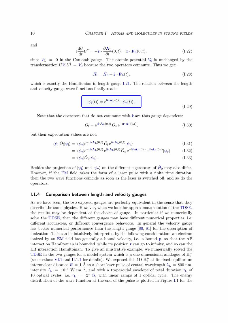
2 at its fixed equilibriuminternuclear distance R = 1 Å to a short laser pulse of central wavelength λL = 800 nm,intensity IL = 1014 W.cm−2, and with a trapezoidal envelope of total duration τL of10 optical cycles, i.e. τL = 27 fs, with linear ramps of 1 optical cycle. The energydistribution of the wave function at the end of the pulse is plotted in Figure I.1 for the
I.1 Time-Dependent Schrödinger Equation 11
1E-10
1E-08
1E-06
1E-04
1E-02
1E+00
−40 −30 −20 −10 0 10 20
Energy
spectrum
(arb.
unit)
E (eV)
ER ∆t = 1.7× 10⁻³ a.u.AP ∆t = 1.3× 10⁻² a.u.ER ∆t = 1.3× 10⁻² a.u.
Figure I.1 Energy distribution of the 1D H+2 at the end of the laser pulse com-
puted with the window method [82] (see section II.3.4).
two different gauges and for different values of the time step ∆t. We see on the figurethat for ∆t = 1.3 × 10⁻² a.u. the results obtained in the velocity (in red) and length(in blue) gauge do not coincide in the positive energy region (the continuum). It seemsthat the final population in the continuum states |ϕE〉 is gauge dependent. However wesaw in the previous section that as soon as the laser is switched off, i.e. at the end of thepulse, then the length and velocity wave functions should coincide. The problem here isthat the length gauge simulation is not converged at a time step ∆t = 1.3 × 10⁻² a.u.,i.e. that the error induced by the propagation algorithm is not negligible. If we performthe same simulation, in length gauge, but at a smaller time step ∆t = 1.7 × 10⁻³ a.u. (inblack on Figure I.1), then the results perfectly agree with the velocity gauge and the twocurves are indistinguishable for the naked eye. This means that, indeed, the numericalsolution in each gauge are equivalent as long as the calculation is converged. Howeverthe length gauge has a slower convergence than the velocity gauge. We just mention thatthis observation is actually restricted to ∆t, the convergence properties with respect to∆x are very simillar for the two gauges.
We may intuitively think that this is related to numerical accuracy (or inaccuracy)problems, i.e. because of the finite precision of real numbers representation in a computer.We investigated this issue by comparing our numerical results where the wave functionis represented on a spatial grid, to numerical simulations performed by Felipe ZapataAbellán during his PhD at the Laboratoire de Chimie Théorique where the wave functionis represented on a B-splines basis set (see section VI.1.2). In both cases, the same prop-agation algorithm is used: a Crank Nicolson (CN) algorithm [83] (see section II.1.2 b)).It is remarkable in Figure I.2 that the results obtained in the grid (in blue) and B-splines
12 Chapter I. Atoms and molecules in strong fields
1E-10
1E-08
1E-06
1E-04
1E-02
1E+00
−40 −30 −20 −10 0 10 20
(a)Velocity gauge
−40 −30 −20 −10 0 10 20
(b)Length gauge
Energy
spectrum
(arb.
unit)
E (eV) E (eV)
B-splinesGrid
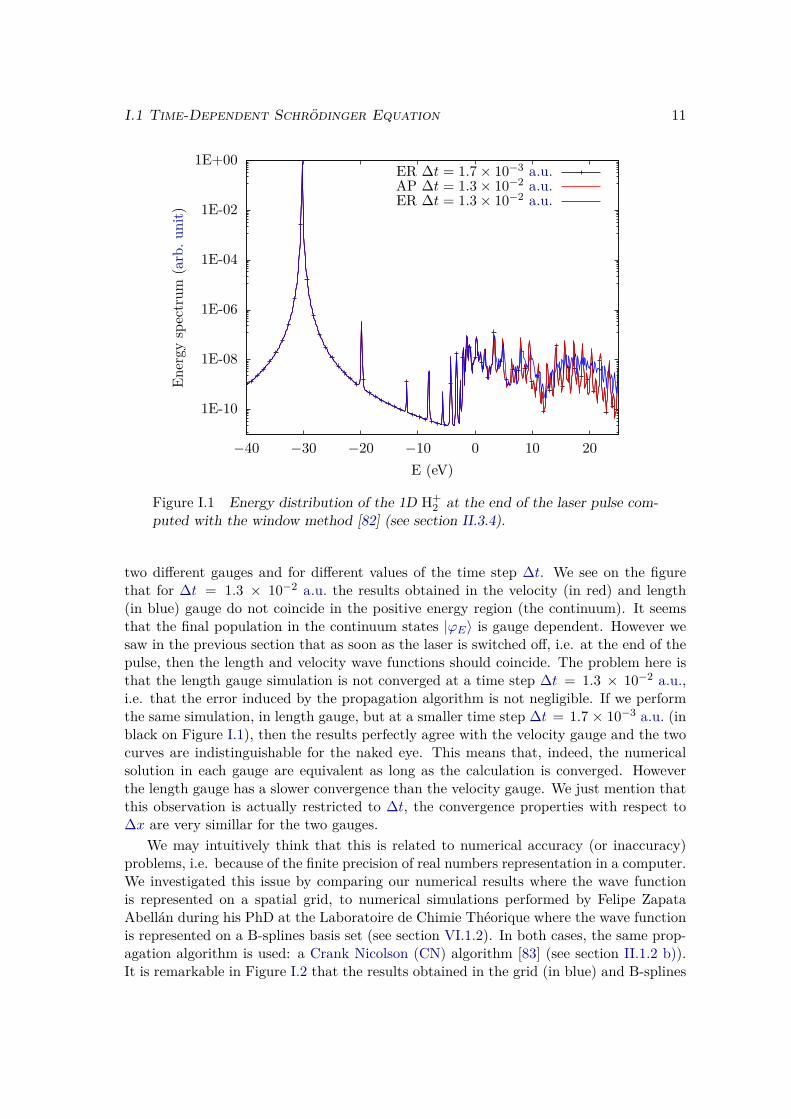
Figure I.2 Energy distribution of the 1D H+2 at the end of the laser pulse com-
puted with a Grid and a B-splines representation and in (a) velocity or (b) lengthgauge. In both cases ∆t = 1.3 × 10⁻² a.u..
(in red) basis sets are identical. The slow convergence of the length gauge numericalsimulation that we just pointed out with the grid is also observed with B-splines. We cantherefore conclude that is is a general feature of the CN propagation algorithm.
These disparities between the two gauges are not restricted to numerical computations,they will also come out when we seek approximate solutions of the TDSE. For example inthe Strong Field Approximation (SFA) framework (see section I.3.3), the results we obtainare actually gauge dependent. The physical interpretation of these approximate methodscan thus be complex, since, as we will see, one of the two gauges may give unphysicalresults in some cases [84]. To overcome these difficulties a gauge independent formulationof the SFA has recently been developped in [85], however we will not discuss it in moredetail in this thesis.
I.2 Time-dependent perturbation theory
When we think of an atom or a molecule interacting with light, in particular in spec-troscopy, we like to think in terms of absorption and emission of one or several photonsby the atom or the molecule. This intuitive picture of light-matter interaction is rooted inthe Time-Dependent Perturbation Theory. No need to say how central this theory is, notonly for the treatment of light-matter interaction, but for any quantum problem involvinga small time-dependent perturbation to a system. The derivation that we present here isgreatly inspired from the well-known book of Cohen-Tannoudji, Diu and Laloë [86].
I.2 Time-dependent perturbation theory 13
I.2.1 General time-dependent perturbation
a) Time-dependent Schrödinger equation in the stationary states basis
In this method we suppose that we know exactly the solutions of a time-independentproblem, i.e. that we know all the eigenstates and eigenvalues of a Hamiltonian H0. Inour case it will be the field-free atomic (or molecular) Hamiltonian for the electron. Wewill consider that, for times t < 0, the perturbation W (t) is zero, so that the initial stateof the system is in an eigenstate |ϕi〉 of H0. At time t = 0 the perturbation is switchedon and the perturbed Hamiltonian reads:
H(t) = H0 + λW (t), (I.34)
where λ 1 and W is comparable to H0. In our case this perturbation λW (t) will bethe interaction Hamiltonian p ·AL(t) or r · FL(t) depending on the choice of gauge.
The initial state |ϕi〉 is no longer a stationary state of the system and the wave functionstarts to evolve under the Hamiltonian (I.34). The point of this section is to describe thedynamics of the perturbed system. We will then be interested in the probability Pif (t)to have a transition from the initial state to a final state |ϕf 〉 after a time t.
The set of all eigenstates of H0 provides a natural basis on which to develop thetime-dependent wave function:
|ψ(t)〉 =∑j
|ϕj〉 〈ϕj |ψ(t)〉 =∑j
cj(t) |ϕj〉 , (I.35)
and the perturbation:
W (t) =∑j,k
|ϕj〉 〈ϕj | W (t) |ϕk〉 〈ϕk| =∑j,k
Wjk(t) |ϕj〉 〈ϕk| . (I.36)
The unperturbed Hamiltonian H0 is diagonal in the |ϕj〉 basis:
H0 =∑j
Ej |ϕj〉 〈ϕj | . (I.37)
Inserting (I.35), (I.36) and (I.37) in the TDSE, we get a system of coupled linear differ-ential equations for the coefficients cj(t):
idcjdt (t) = Ejcj(t) + λ∑k
Wjk(t)ck(t). (I.38)
We can get rid of the H0 contribution to the dynamics by moving to the interactionrepresentation with respect to H0, i.e. by performing the unitary transform
|ψ(t)〉 = eiH0t |ψ(t)〉 . (I.39)
In this representation, the coefficients become:
cj(t) = eiEjt cj(t). (I.40)
14 Chapter I. Atoms and molecules in strong fields
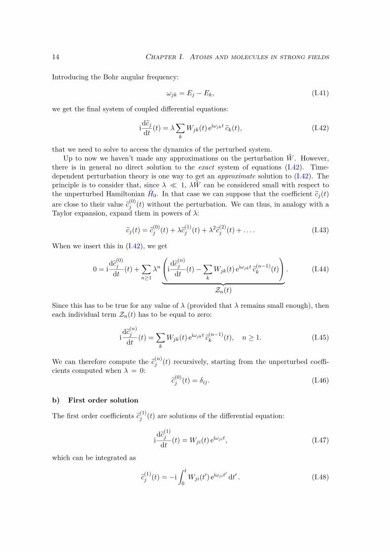
Introducing the Bohr angular frequency:
ωjk = Ej − Ek, (I.41)
we get the final system of coupled differential equations:
idcjdt (t) = λ∑k
Wjk(t) eiωjkt ck(t), (I.42)
that we need to solve to access the dynamics of the perturbed system.Up to now we haven’t made any approximations on the perturbation W . However,
there is in general no direct solution to the exact system of equations (I.42). Time-dependent perturbation theory is one way to get an approximate solution to (I.42). Theprinciple is to consider that, since λ 1, λW can be considered small with respect tothe unperturbed Hamiltonian H0. In that case we can suppose that the coefficient cj(t)are close to their value c(0)
j (t) without the perturbation. We can thus, in analogy with aTaylor expansion, expand them in powers of λ:
cj(t) = c(0)j (t) + λc
(1)j (t) + λ2c
(2)j (t) + . . . . (I.43)
When we insert this in (I.42), we get
0 = idc(0)j
dt (t) +∑n≥1
λn
idc(n)j
dt (t)−∑k
Wjk(t) eiωjkt c(n−1)k (t)
︸ ︷︷ ︸
Zn(t)
. (I.44)
Since this has to be true for any value of λ (provided that λ remains small enough), theneach individual term Zn(t) has to be equal to zero:
idc(n)j
dt (t) =∑k
Wjk(t) eiωjkt c(n−1)k (t), n ≥ 1. (I.45)
We can therefore compute the c(n)j (t) recursively, starting from the unperturbed coeffi-
cients computed when λ = 0:c
(0)j (t) = δij . (I.46)
b) First order solution
The first order coefficients c(1)j (t) are solutions of the differential equation:
idc(1)j
dt (t) = Wji(t) eiωjit, (I.47)
which can be integrated as
c(1)j (t) = −i
∫ t
0Wji(t′) eiωjit′ dt′ . (I.48)
I.2 Time-dependent perturbation theory 15
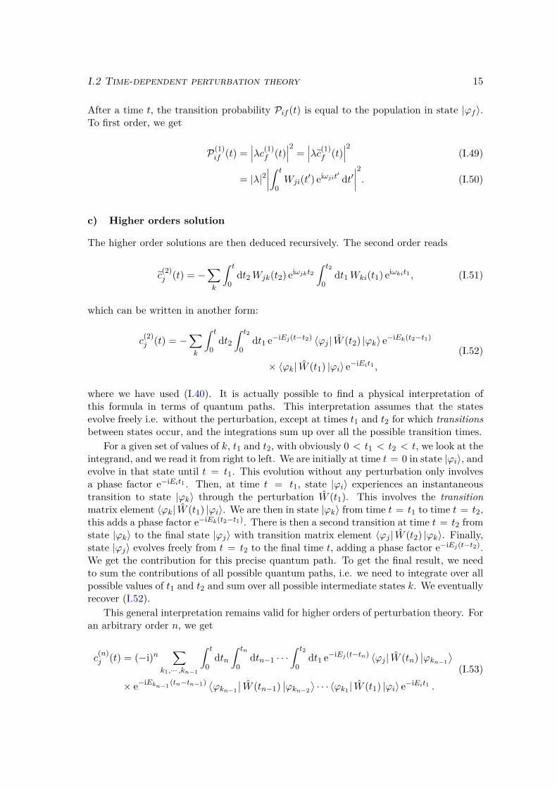
After a time t, the transition probability Pif (t) is equal to the population in state |ϕf 〉.To first order, we get
P(1)if (t) =
∣∣∣λc(1)f (t)
∣∣∣2 =∣∣∣λc(1)
f (t)∣∣∣2 (I.49)
= |λ|2∣∣∣∣∫ t
0Wji(t′) eiωjit′ dt′
∣∣∣∣2. (I.50)
c) Higher orders solution
The higher order solutions are then deduced recursively. The second order reads
c(2)j (t) = −
∑k
∫ t
0dt2Wjk(t2) eiωjkt2
∫ t2
0dt1Wki(t1) eiωkit1 , (I.51)
which can be written in another form:
c(2)j (t) = −
∑k
∫ t
0dt2
∫ t2
0dt1 e−iEj(t−t2) 〈ϕj | W (t2) |ϕk〉 e−iEk(t2−t1)
× 〈ϕk| W (t1) |ϕi〉 e−iEit1 ,
(I.52)
where we have used (I.40). It is actually possible to find a physical interpretation ofthis formula in terms of quantum paths. This interpretation assumes that the statesevolve freely i.e. without the perturbation, except at times t1 and t2 for which transitionsbetween states occur, and the integrations sum up over all the possible transition times.
For a given set of values of k, t1 and t2, with obviously 0 < t1 < t2 < t, we look at theintegrand, and we read it from right to left. We are initially at time t = 0 in state |ϕi〉, andevolve in that state until t = t1. This evolution without any perturbation only involvesa phase factor e−iEit1 . Then, at time t = t1, state |ϕi〉 experiences an instantaneoustransition to state |ϕk〉 through the perturbation W (t1). This involves the transitionmatrix element 〈ϕk| W (t1) |ϕi〉. We are then in state |ϕk〉 from time t = t1 to time t = t2,this adds a phase factor e−iEk(t2−t1). There is then a second transition at time t = t2 fromstate |ϕk〉 to the final state |ϕj〉 with transition matrix element 〈ϕj | W (t2) |ϕk〉. Finally,state |ϕj〉 evolves freely from t = t2 to the final time t, adding a phase factor e−iEj(t−t2).We get the contribution for this precise quantum path. To get the final result, we needto sum the contributions of all possible quantum paths, i.e. we need to integrate over allpossible values of t1 and t2 and sum over all possible intermediate states k. We eventuallyrecover (I.52).
This general interpretation remains valid for higher orders of perturbation theory. Foran arbitrary order n, we get
c(n)j (t) = (−i)n
∑k1,··· ,kn−1
∫ t
0dtn
∫ tn
0dtn−1 · · ·
∫ t2
0dt1 e−iEj(t−tn) 〈ϕj | W (tn)
∣∣ϕkn−1
⟩× e−iEkn−1 (tn−tn−1) ⟨ϕkn−1
∣∣ W (tn−1)∣∣ϕkn−2
⟩· · · 〈ϕk1 | W (t1) |ϕi〉 e−iEit1 .
(I.53)
16 Chapter I. Atoms and molecules in strong fields
I.2.2 Perturbation by an electromagnetic field
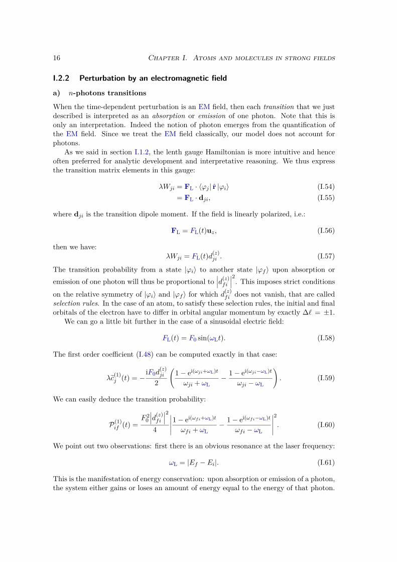
a) n-photons transitions
When the time-dependent perturbation is an EM field, then each transition that we justdescribed is interpreted as an absorption or emission of one photon. Note that this isonly an interpretation. Indeed the notion of photon emerges from the quantification ofthe EM field. Since we treat the EM field classically, our model does not account forphotons.
As we said in section I.1.2, the lenth gauge Hamiltonian is more intuitive and henceoften preferred for analytic development and interpretative reasoning. We thus expressthe transition matrix elements in this gauge:
λWji = FL · 〈ϕj | r |ϕi〉 (I.54)= FL · dji, (I.55)
where dji is the transition dipole moment. If the field is linearly polarized, i.e.:
FL = FL(t)uz, (I.56)
then we have:λWji = FL(t)d(z)
ji . (I.57)
The transition probability from a state |ϕi〉 to another state |ϕf 〉 upon absorption oremission of one photon will thus be proportional to
∣∣∣d(z)fi
∣∣∣2. This imposes strict conditionson the relative symmetry of |ϕi〉 and |ϕf 〉 for which d(z)
fi does not vanish, that are calledselection rules. In the case of an atom, to satisfy these selection rules, the initial and finalorbitals of the electron have to differ in orbital angular momentum by exactly ∆` = ±1.
We can go a little bit further in the case of a sinusoidal electric field:
FL(t) = F0 sin(ωLt). (I.58)
The first order coefficient (I.48) can be computed exactly in that case:
λc(1)j (t) = −
iF0d(z)ji
2
(1− ei(ωji+ωL)t
ωji + ωL− 1− ei(ωji−ωL)t
ωji − ωL
). (I.59)
We can easily deduce the transition probability:
P(1)if (t) =
F 20
∣∣∣d(z)fi
∣∣∣24
∣∣∣∣∣1− ei(ωfi+ωL)t
ωfi + ωL− 1− ei(ωfi−ωL)t
ωfi − ωL
∣∣∣∣∣2
. (I.60)
We point out two observations: first there is an obvious resonance at the laser frequency:
ωL = |Ef − Ei|. (I.61)
This is the manifestation of energy conservation: upon absorption or emission of a photon,the system either gains or loses an amount of energy equal to the energy of that photon.
I.2 Time-dependent perturbation theory 17
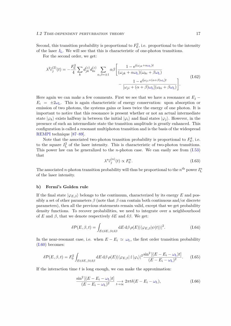
Second, this transition probability is proportional to F 20 , i.e. proportional to the intensity
of the laser IL. We will see that this is characteristic of one-photon transitions.For the second order, we get:
λ2c(2)j (t) = −F
20
4∑k
d(z)jk d
(z)ki
∑α,β=±1
αβ
[1− ei(ωjk+αωL)t
(ωjk + αωL)(ωki + βωL)
− 1− ei[ωji+(α+β)ωL]t
[ωji + (α+ β)ωL](ωki + βωL)
].
(I.62)
Here again we can make a few comments. First we see that we have a resonance at Ej −Ei = ±2ωL. This is again characteristic of energy conservation: upon absorption oremission of two photons, the systems gains or loses twice the energy of one photon. It isimportant to notice that this resonance is present whether or not an actual intermediatestate |ϕk〉 exists halfway in between the initial |ϕi〉 and final states |ϕj〉. However, in thepresence of such an intermediate state the transition amplitude is greatly enhanced. Thisconfiguration is called a resonant multiphoton transition and is the basis of the widespreadREMPI technique [87–89].
Note that the associated two-photon transition probability is proportional to F 40 , i.e.
to the square I2L of the laser intensity. This is characteristic of two-photon transitions.
This power law can be generalized to the n-photon case. We can easily see from (I.53)that
λnc(n)j (t) ∝ Fn0 . (I.63)
The associated n-photon transition probability will thus be proportional to the nth power InLof the laser intensity.
b) Fermi’s Golden rule
If the final state |ϕE,β〉 belongs to the continuum, characterized by its energy E and pos-sibly a set of other parameters β (note that β can contain both continuous and/or discreteparameters), then all the previous statements remain valid, except that we get probabilitydensity functions. To recover probabilities, we need to integrate over a neighbourhoodof E and β, that we denote respectively δE and δβ. We get:
δP(E, β, t) =∫E∈δE, β∈δβ
dE dβ ρ(E)|〈ϕE,β|ψ(t)〉|2. (I.64)
In the near-resonant case, i.e. when E − Ei ' ωL, the first order transition probability(I.60) becomes:
δP(E, β, t) = F 20
∫E∈δE, β∈δβ
dE dβ ρ(E)|〈ϕE,β| z |ϕi〉|2sin2 [(E − Ei − ωL)t]
(E − Ei − ωL)2 . (I.65)
If the interaction time t is long enough, we can make the approximation:
sin2 [(E − Ei − ωL)t](E − Ei − ωL)2 −→
t→∞2πtδ(E − Ei − ωL), (I.66)
18 Chapter I. Atoms and molecules in strong fields
and if δβ is small enough, we get:
δP(E, β, t) =F 2
0 δβ|〈ϕEi+ωL,β| z |ϕi〉|2ρ(Ei + ωL)t if Ei + ωL ∈ δE
0 if Ei + ωL /∈ δE(I.67)
Differentiating this expression with respect to time, we recover the well known Fermi’sGolden rule.
c) Illustrative example
To show the characteristic features of n-photon transitions, we consider a very simplesystem: an electron trapped in a one dimensional Gaussian potential well:
V0(x) = − ex22 . (I.68)
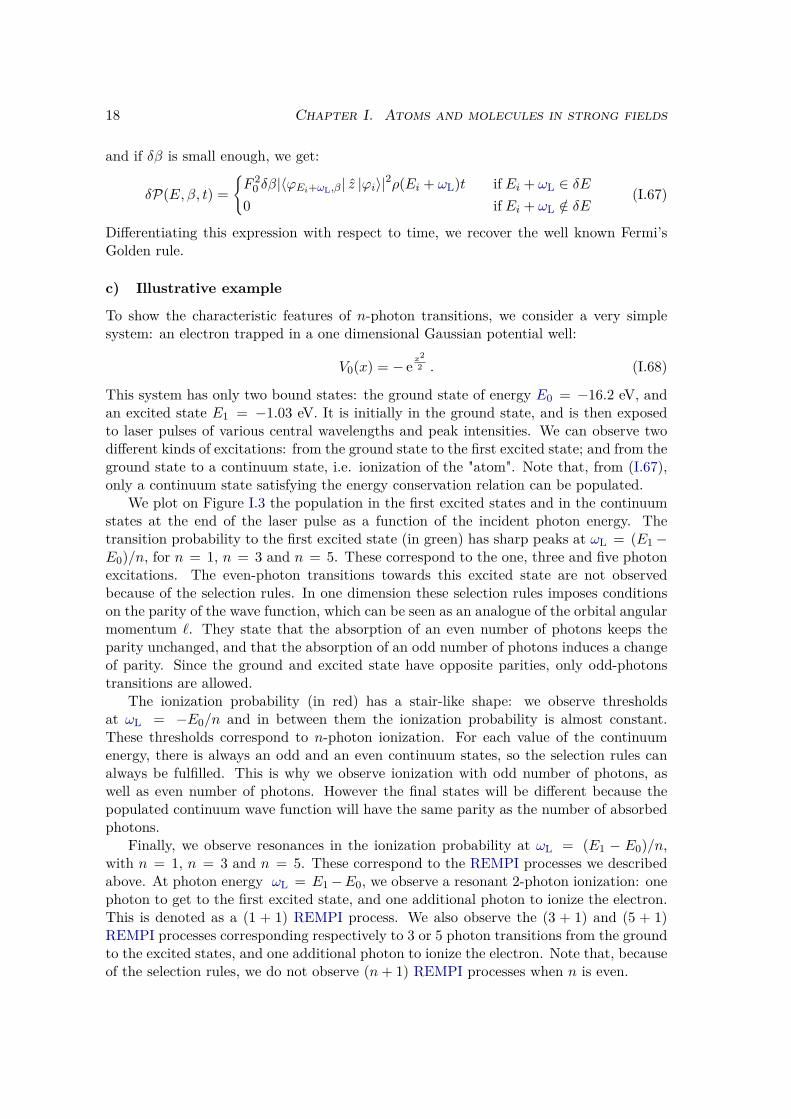
This system has only two bound states: the ground state of energy E0 = −16.2 eV, andan excited state E1 = −1.03 eV. It is initially in the ground state, and is then exposedto laser pulses of various central wavelengths and peak intensities. We can observe twodifferent kinds of excitations: from the ground state to the first excited state; and from theground state to a continuum state, i.e. ionization of the "atom". Note that, from (I.67),only a continuum state satisfying the energy conservation relation can be populated.
We plot on Figure I.3 the population in the first excited states and in the continuumstates at the end of the laser pulse as a function of the incident photon energy. Thetransition probability to the first excited state (in green) has sharp peaks at ωL = (E1−E0)/n, for n = 1, n = 3 and n = 5. These correspond to the one, three and five photonexcitations. The even-photon transitions towards this excited state are not observedbecause of the selection rules. In one dimension these selection rules imposes conditionson the parity of the wave function, which can be seen as an analogue of the orbital angularmomentum `. They state that the absorption of an even number of photons keeps theparity unchanged, and that the absorption of an odd number of photons induces a changeof parity. Since the ground and excited state have opposite parities, only odd-photonstransitions are allowed.
The ionization probability (in red) has a stair-like shape: we observe thresholdsat ωL = −E0/n and in between them the ionization probability is almost constant.These thresholds correspond to n-photon ionization. For each value of the continuumenergy, there is always an odd and an even continuum states, so the selection rules canalways be fulfilled. This is why we observe ionization with odd number of photons, aswell as even number of photons. However the final states will be different because thepopulated continuum wave function will have the same parity as the number of absorbedphotons.
Finally, we observe resonances in the ionization probability at ωL = (E1 − E0)/n,with n = 1, n = 3 and n = 5. These correspond to the REMPI processes we describedabove. At photon energy ωL = E1−E0, we observe a resonant 2-photon ionization: onephoton to get to the first excited state, and one additional photon to ionize the electron.This is denoted as a (1 + 1) REMPI process. We also observe the (3 + 1) and (5 + 1)REMPI processes corresponding respectively to 3 or 5 photon transitions from the groundto the excited states, and one additional photon to ionize the electron. Note that, becauseof the selection rules, we do not observe (n+ 1) REMPI processes when n is even.
I.3 High Harmonic Generation and Strong Field Approximation 19
1E-14
1E-12
1E-10
1E-08
1E-06
1E-04
1E-02
1E+00
2 4 6 8 10 12 14 16 18
3ph
2ph
1 photon
4ph
5ph
6ph
6.1 8.7 16.9
Tran
sitionprob
ability
ω (eV)
Ionization1st excited state
Figure I.3 Absorption spectrum of an electron in a Gaussian potential well(I.68), exposed to a sine square envelope laser pulse of 200 optical cycles and ofpeak intensity IL = 3.5 × 10¹² W.cm−2 computed by solving the TDSE (seesection II.1.1). In red the ionization probability at the end of the pulse, in greenthe population in the first excited state at the end of the pulse. The number ofphotons for each ionization threshold is displayed.
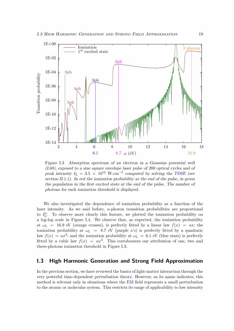
We also investigated the dependence of ionization probability as a function of thelaser intensity. As we said before, n-photon transition probabilities are proportionalto InL . To observe more clearly this feature, we plotted the ionization probability ona log-log scale in Figure I.4. We observe that, as expected, the ionization probabilityat ωL = 16.9 eV (orange crosses), is perfectly fitted by a linear law f(x) = ax; theionization probability at ωL = 8.7 eV (purple x’s) is perfectly fitted by a quadraticlaw f(x) = ax2; and the ionization probability at ωL = 6.1 eV (blue stars) is perfectlyfitted by a cubic law f(x) = ax3. This corroborates our attribution of one, two andthree-photons ionization threshold in Figure I.3.
I.3 High Harmonic Generation and Strong Field Approximation
In the previous section, we have reviewed the basics of light-matter interaction through thevery powerful time-dependent perturbation theory. However, as its name indicates, thismethod is relevant only in situations where the EM field represents a small perturbationto the atomic or molecular system. This restricts its range of applicability to low intensity
20 Chapter I. Atoms and molecules in strong fields
1E-12
1E-10
1E-08
1E-06
1E-04
1E-02
1E+00
1E+09 1E+10 1E+11 1E+12
slope 1
slope 2
slope 3Ionizatio
nprob
ability
IL (W.cm−2)
ωL = 16.9 eVωL = 8.7 eVωL = 6.1 eV
Figure I.4 Ionization probability as a function of the laser pulse intensity forthree different photon energies (indicated in Figure I.3) computed by solvingthe TDSE (see section II.1.1). The system and laser pulse are the same as inFigure I.3. The dots are the results of the numerical simulations, and the linesare power law fits.
and high frequency laser fields. When the laser intensity is too high, compared to thestrengh of the electron-nuclei interaction, then the electric field substantially distorts theatomic potential so that the electron may escape through tunnel effect. This highly non-linear effect, called tunnel ionization, is the first step of many strong field processes suchas HHG [90, 91], ATI [92, 93] or non-sequential multiple ionization [94].
The distinctive feature of these strong field processes is their extreme non-linearity,which is inherited from their common first step, i.e. tunnel ionization. This first stepcannot be accounted for by perturbation theory, i.e. by the description in terms of oneor several photon transitions. This strong field regime, or tunnel regime, is the source ofcompletely different physical phenomena. The description, analysis, and interpretation ofthese new phenomena thus relies on specific tools, and specific physical models.
In this thesis we are mainly interested in HHG, which is the subject of the presentsection. This particular process present many different aspects, both experimental andtheoretical. It is, together with the XRay free electron lasers (XFEL), one of the onlysource of attosecond coherent light pulses [95–97], and is therefore at the heart of manyattosecond-resolution time resolved experiments [32, 33, 50, 22, 27, 29]. It is also apowerful self-probe of the chemical species that generate the harmonics. Indeed, it allowsto reconstruct the dynamics of the emitting system both temporally and spatially withÅngström and attosecond resolution [59, 98, 99, 45, 41]. This multiplicity of experimentsrequires advanced theory, not only in the form of numerical simulations that are necessary
I.3 High Harmonic Generation and Strong Field Approximation 21
for the quantitative analysis of experimental results, but also in the form of analyticintuitive physical models that are valuable for the description, interpretation and designof experiments.
In this section, we first present a phenomenological approach to HHG, then we detaila very powerful model that describes HHG in the Strong Field Approximation (SFA):the so-called Lewenstein model [11]. Though HHG has also been observed and used insolids [100–102], nanoscale strucures [103, 104] and liquids [105], in this thesis we focuson the gas phase. We will describe the process at a single atom (or molecule) level. Thephysical models that we can construct at this level of description constitute the groundfor all the qualitative physical pictures and interpretations we have of HHG. To get morequantitative results it is then necessary to include macroscopic collective effects [106, 90,96, 107, 108], such as phase matching between the different emitters, inhomogeneity inthe gas, or spatial dependency of the laser intensity close to the focus area. However,the accurate quantitative computation of HHG still remains a challenge for theoreticians.We will therefore concentrate on physical insight, rather than on quantitative accuracyas such.
I.3.1 What is High order Harmonic Generation ?
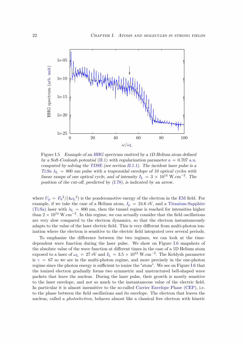
When a short laser pulse of a few tens of fs, with Infrared (IR) or mid-IR central wave-length, and high intensity IL ∼ 1014 − 1015 W.cm−2, is focused on a gas jet, then weobserve that this gas re-emits a radiation [7, 8, 109–111]. This radiation has very peculiarcharacteristics, as can be seen from the typical spectrum in Figure I.5. This spectrumwas computed with the numerical methods detailed in sections II.1.1 and II.3.2. First it isvery large, spreading from the IR to the XUV domain, which enlightens the non-linearityof the process. Second, it is shaped as a train of very short pulses of a few tens of as[95, 112]. Third, its spectrum is only composed of the odd harmonics (2p + 1)ωL of theincident laser frequency. All these odd harmonics have almost the same intensity, fromharmonic 1 to a cut-off value that is generally around a few tens but than can go upto a few hundreds in some conditions. Above this cut-off energy (around harmonic 52on Figure I.5, indicated by an arrow) the harmonic intensity sharply decreases. The lastcharacteristic is that this radiation is coherent [107].
From all those very promising characteristics, it is quite easy to understand the pop-ularity of HHG as a light source. However it is not so easy at first sight to understandthe mechanism creating this radiation. We can first observe that, in the conditions citedabove, we are in the tunnel regime and not in the perturbative regime. Or, said oth-erwise, ionization is dominated by tunnel ionization rather than multiphoton ionization.The limit between these two regimes is in practice measured by the Keldysh parame-ter γ [113]. It is defined as the ratio of the so-called "tunnelling time", i.e. the time theelectron takes to tunnel out of the potential barrier, to half a laser period. From thisdefinition we see that we will be in the tunnel regime if γ 1, i.e. if the electron hasenough time in half a laser period to tunnel out. On the contrary, for γ 1 we will bein the multi-photon regime. The formal expression of the Keldysh parameter reads
γ =√
Ip2Up
, (I.69)
22 Chapter I. Atoms and molecules in strong fields
1e-25
1e-20
1e-15
1e-10
1e-05
0 20 40 60 80 100
HHG
spectrum
(arb.
unit)
ω/ωL
Figure I.5 Example of an HHG spectrum emitted by a 1D Helium atom definedby a Soft-Coulomb potential (II.1) with regularization parameter a = 0.707 a.u.computed by solving the TDSE (see section II.1.1). The incident laser pulse is aTi:Sa λL = 800 nm pulse with a trapezoidal envelope of 10 optical cycles withlinear ramps of one optical cycle, and of intensity IL = 3 × 10¹⁴ W.cm−2. Theposition of the cut-off, predicted by (I.78), is indicated by an arrow.
where Up = F02/(4ωL
2) is the ponderomotive energy of the electron in the EM field. Forexample, if we take the case of a Helium atom, Ip = 24.6 eV, and a Titanium-Sapphire(Ti:Sa) laser with λL = 800 nm, then the tunnel regime is reached for intensities higherthan 2 × 10¹⁴ W.cm−2. In this regime, we can actually consider that the field oscillationsare very slow compared to the electron dynamics, so that the electron instantaneouslyadapts to the value of the laser electric field. This is very different from multi-photon ion-ization where the electron is sensitive to the electric field integrated over several periods.
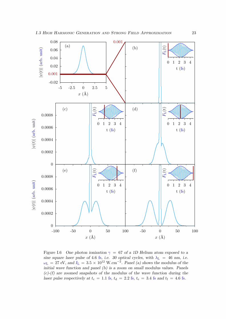
To emphasize the difference between the two regimes, we can look at the time-dependent wave function during the laser pulse. We show on Figure I.6 snapshots ofthe absolute value of the wave function at different times in the case of a 1D Helium atomexposed to a laser of ωL = 27 eV and IL = 3.5 × 10¹² W.cm−2. The Keldysh parameteris γ = 67 so we are in the multi-photon regime, and more precisely in the one-photonregime since the photon energy is sufficient to ionize the "atom". We see on Figure I.6 thatthe ionized electron gradually forms two symmetric and unstructured bell-shaped wavepackets that leave the nucleus. During the laser pulse, their growth is mostly sensitiveto the laser envelope, and not so much to the instantaneous value of the electric field.In particular it is almost insensitive to the so-called Carrier Envelope Phase (CEP), i.e.to the phase between the field oscillations and its envelope. The electron that leaves thenucleus, called a photoelectron, behaves almost like a classical free electron with kinetic
I.3 High Harmonic Generation and Strong Field Approximation 23
-0.02
0.001
0.02
0.04
0.06
0.08
-5 -2.5 0 2.5 5
(a)0.001
(b)
0 1 2 3 4
0
0.0002
0.0004
0.0006
0.0008(c)
0 1 2 3 4
(d)
0 1 2 3 4
0
0.0002
0.0004
0.0006
0.0008
-100 -50 0 50 100
(e)
0 1 2 3 4
-50 0 50 100
(f)
0 1 2 3 4
|ψ(t
)|(a
rb.
unit)
x (Å)
FL(t)
t (fs)
|ψ(t
)|(a
rb.
unit)
FL(t)
t (fs)
FL(t)
t (fs)
|ψ(t
)|(a
rb.
unit)
x (Å)
FL(t)
t (fs)
x (Å)
FL(t)
t (fs)
Figure I.6 One photon ionization γ = 67 of a 1D Helium atom exposed to asine square laser pulse of 4.6 fs, i.e. 30 optical cycles, with λL = 46 nm, i.e.ωL = 27 eV, and IL = 3.5 × 10¹² W.cm−2. Panel (a) shows the modulus of theinitial wave function and panel (b) is a zoom on small modulus values. Panels(c)-(f) are zoomed snapshots of the modulus of the wave function during thelaser pulse respectively at tc = 1.1 fs, td = 2.2 fs, te = 3.4 fs and tf = 4.6 fs.
24 Chapter I. Atoms and molecules in strong fields
ωL
|ϕ0〉
|ϕE=E0+ωL〉
V0
(a)
|ϕ0〉
|ϕE=E0+ωL〉
V0
(b)
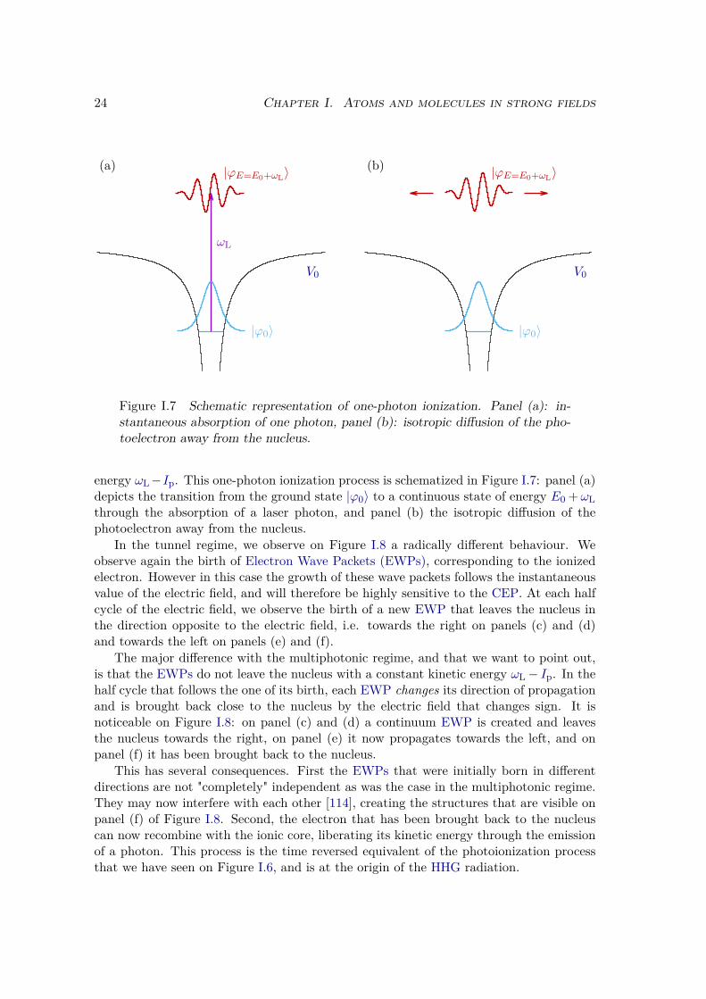
Figure I.7 Schematic representation of one-photon ionization. Panel (a): in-stantaneous absorption of one photon, panel (b): isotropic diffusion of the pho-toelectron away from the nucleus.
energy ωL−Ip. This one-photon ionization process is schematized in Figure I.7: panel (a)depicts the transition from the ground state |ϕ0〉 to a continuous state of energy E0 +ωLthrough the absorption of a laser photon, and panel (b) the isotropic diffusion of thephotoelectron away from the nucleus.
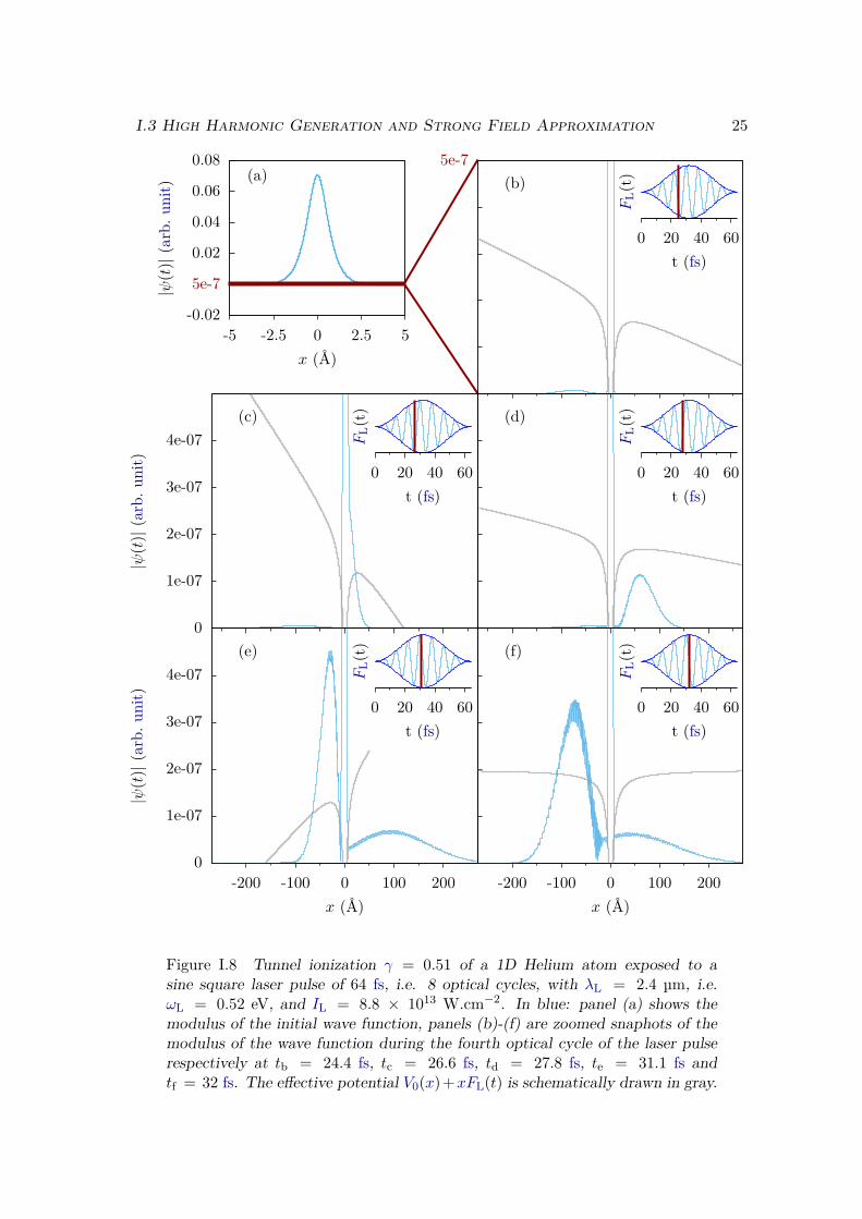
In the tunnel regime, we observe on Figure I.8 a radically different behaviour. Weobserve again the birth of Electron Wave Packets (EWPs), corresponding to the ionizedelectron. However in this case the growth of these wave packets follows the instantaneousvalue of the electric field, and will therefore be highly sensitive to the CEP. At each halfcycle of the electric field, we observe the birth of a new EWP that leaves the nucleus inthe direction opposite to the electric field, i.e. towards the right on panels (c) and (d)and towards the left on panels (e) and (f).
The major difference with the multiphotonic regime, and that we want to point out,is that the EWPs do not leave the nucleus with a constant kinetic energy ωL− Ip. In thehalf cycle that follows the one of its birth, each EWP changes its direction of propagationand is brought back close to the nucleus by the electric field that changes sign. It isnoticeable on Figure I.8: on panel (c) and (d) a continuum EWP is created and leavesthe nucleus towards the right, on panel (e) it now propagates towards the left, and onpanel (f) it has been brought back to the nucleus.
This has several consequences. First the EWPs that were initially born in differentdirections are not "completely" independent as was the case in the multiphotonic regime.They may now interfere with each other [114], creating the structures that are visible onpanel (f) of Figure I.8. Second, the electron that has been brought back to the nucleuscan now recombine with the ionic core, liberating its kinetic energy through the emissionof a photon. This process is the time reversed equivalent of the photoionization processthat we have seen on Figure I.6, and is at the origin of the HHG radiation.
I.3 High Harmonic Generation and Strong Field Approximation 25
-0.02
5e-7
0.02
0.04
0.06
0.08
-5 -2.5 0 2.5 5
(a)5e-7
(b)
0 20 40 60
0
1e-07
2e-07
3e-07
4e-07(c)
0 20 40 60
(d)
0 20 40 60
0
1e-07
2e-07
3e-07
4e-07
-200 -100 0 100 200
(e)
0 20 40 60
-200 -100 0 100 200
(f)
0 20 40 60
|ψ(t
)|(a
rb.
unit)
x (Å)
FL(t)
t (fs)
|ψ(t
)|(a
rb.
unit)
FL(t)
t (fs)
FL(t)
t (fs)
|ψ(t
)|(a
rb.
unit)
x (Å)
FL(t)
t (fs)
x (Å)
FL(t)
t (fs)
Figure I.8 Tunnel ionization γ = 0.51 of a 1D Helium atom exposed to asine square laser pulse of 64 fs, i.e. 8 optical cycles, with λL = 2.4 µm, i.e.ωL = 0.52 eV, and IL = 8.8 × 10¹³ W.cm−2. In blue: panel (a) shows themodulus of the initial wave function, panels (b)-(f) are zoomed snaphots of themodulus of the wave function during the fourth optical cycle of the laser pulserespectively at tb = 24.4 fs, tc = 26.6 fs, td = 27.8 fs, te = 31.1 fs andtf = 32 fs. The effective potential V0(x)+xFL(t) is schematically drawn in gray.
26 Chapter I. Atoms and molecules in strong fields
(a)
|ϕ0〉
V0 + xFL(t)
(b)(b) (c)
ωe
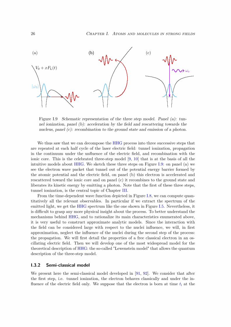
Figure I.9 Schematic representation of the three step model. Panel (a): tun-nel ionization, panel (b): acceleration by the field and rescattering towards thenucleus, panel (c): recombination to the ground state and emission of a photon.
We thus saw that we can decompose the HHG process into three successive steps thatare repeated at each half cycle of the laser electric field: tunnel ionization, propagationin the continuum under the unfluence of the electric field, and recombination with theionic core. This is the celebrated three-step model [9, 10] that is at the basis of all theintuitive models about HHG. We sketch these three steps on Figure I.9: on panel (a) wesee the electron wave packet that tunnel out of the potential energy barrier formed bythe atomic potential and the electric field, on panel (b) this electron is accelerated andrescattered toward the ionic core and on panel (c) it recombines to the ground state andliberates its kinetic energy by emitting a photon. Note that the first of these three steps,tunnel ionization, is the central topic of Chapter III.
From the time-dependent wave function depicted in Figure I.8, we can compute quan-titatively all the relevant observables. In particular if we extract the spectrum of theemitted light, we get the HHG spectrum like the one shown in Figure I.5. Nevertheless, itis difficult to grasp any more physical insight about the process. To better understand themechanisms behind HHG, and to rationalize its main characteristics enumerated above,it is very useful to construct approximate analytic models. Since the interaction withthe field can be considered large with respect to the nuclei influence, we will, in firstapproximation, neglect the influence of the nuclei during the second step of the process:the propagation. We will first detail the properties of a free classical electron in an os-cillating electric field. Then we will develop one of the most widespread model for thetheoretical description of HHG: the so-called "Lewenstein model" that allows the quantumdescription of the three-step model.
I.3.2 Semi-classical model
We present here the semi-classical model developed in [91, 92]. We consider that afterthe first step, i.e. tunnel ionization, the electron behaves classically and under the in-fluence of the electric field only. We suppose that the electron is born at time ti at the
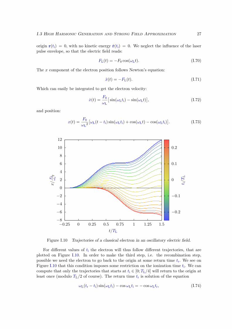
I.3 High Harmonic Generation and Strong Field Approximation 27
origin r(ti) = 0, with no kinetic energy r(ti) = 0. We neglect the influence of the laserpulse envelope, so that the electric field reads:
FL(t) = −F0 cos(ωLt). (I.70)
The x component of the electron position follows Newton’s equation:
x(t) = −FL(t). (I.71)
Which can easily be integrated to get the electron velocity:
x(t) = F0ωL
[sin(ωLti)− sin(ωLt)
], (I.72)
and position:
x(t) = F0ωL2
[ωL(t− ti) sin(ωLti) + cos(ωLt)− cos(ωLti)
]. (I.73)
−8
−6
−4
−2
0
2
4
6
8
10
12
−0.25 0 0.25 0.5 0.75 1 1.25 1.5
x/F
0ω
L2
t/TL
−0.2
−0.1
0
0.1
0.2
t i/T
L
Figure I.10 Trajectories of a classical electron in an oscillatory electric field.
For different values of ti the electron will thus follow different trajectories, that areplotted on Figure I.10. In order to make the third step, i.e. the recombination step,possible we need the electron to go back to the origin at some return time tr. We see onFigure I.10 that this condition imposes some restriction on the ionization time ti. We cancompute that only the trajectories that starts at ti ∈ [0;TL/4] will return to the origin atleast once (modulo TL/2 of course). The return time tr is solution of the equation
ωL(tr − ti) sin(ωLti)− cosωLti = − cosωLtr, (I.74)
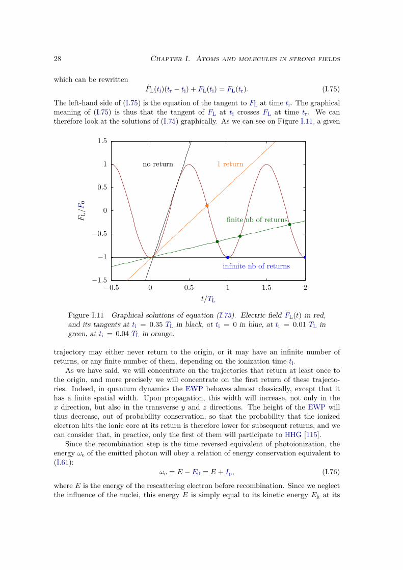
28 Chapter I. Atoms and molecules in strong fields
which can be rewrittenFL(ti)(tr − ti) + FL(ti) = FL(tr). (I.75)
The left-hand side of (I.75) is the equation of the tangent to FL at time ti. The graphicalmeaning of (I.75) is thus that the tangent of FL at ti crosses FL at time tr. We cantherefore look at the solutions of (I.75) graphically. As we can see on Figure I.11, a given
−1.5
−1
−0.5
0
0.5
1
1.5
−0.5 0 0.5 1 1.5 2
no return 1 return
infinite nb of returns
FL/F
0
t/TL
finite nb of returns
Figure I.11 Graphical solutions of equation (I.75). Electric field FL(t) in red,and its tangents at ti = 0.35 TL in black, at ti = 0 in blue, at ti = 0.01 TL ingreen, at ti = 0.04 TL in orange.
trajectory may either never return to the origin, or it may have an infinite number ofreturns, or any finite number of them, depending on the ionization time ti.
As we have said, we will concentrate on the trajectories that return at least once tothe origin, and more precisely we will concentrate on the first return of these trajecto-ries. Indeed, in quantum dynamics the EWP behaves almost classically, except that ithas a finite spatial width. Upon propagation, this width will increase, not only in thex direction, but also in the transverse y and z directions. The height of the EWP willthus decrease, out of probability conservation, so that the probability that the ionizedelectron hits the ionic core at its return is therefore lower for subsequent returns, and wecan consider that, in practice, only the first of them will participate to HHG [115].
Since the recombination step is the time reversed equivalent of photoionization, theenergy ωe of the emitted photon will obey a relation of energy conservation equivalent to(I.61):
ωe = E − E0 = E + Ip, (I.76)
where E is the energy of the rescattering electron before recombination. Since we neglectthe influence of the nuclei, this energy E is simply equal to its kinetic energy Ek at its
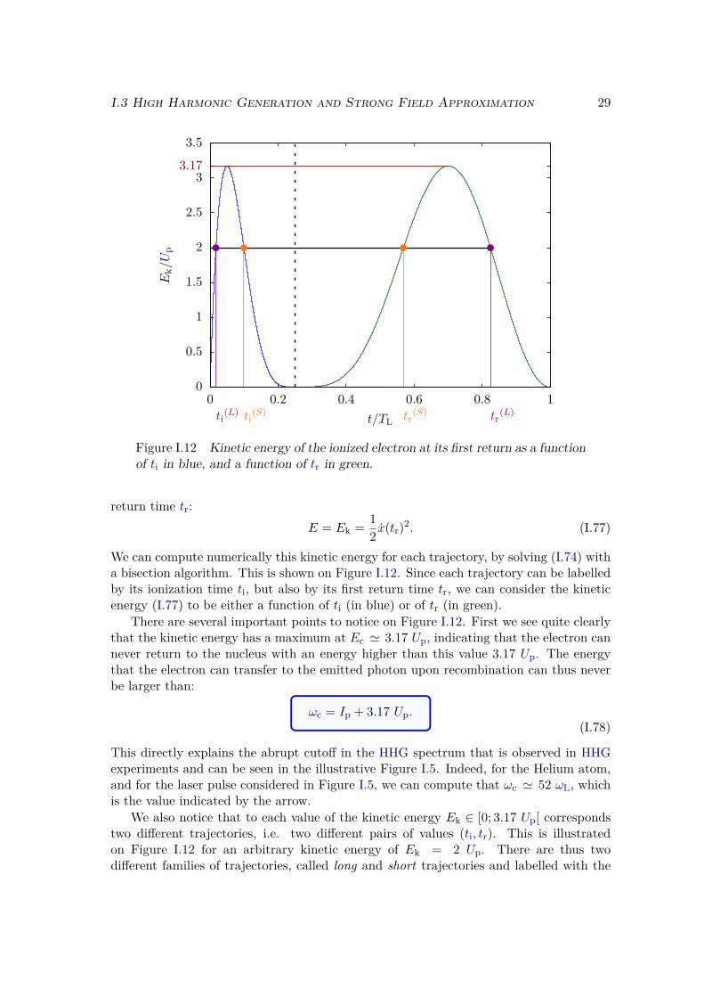
I.3 High Harmonic Generation and Strong Field Approximation 29
3.17
0
0.5
1
1.5
2
2.5
3
3.5
0 0.2 0.4 0.6 0.8 1ti
(L) ti(S) tr
(S) tr(L)
Ek/U
p
t/TL
Figure I.12 Kinetic energy of the ionized electron at its first return as a functionof ti in blue, and a function of tr in green.
return time tr:E = Ek = 1
2 x(tr)2. (I.77)
We can compute numerically this kinetic energy for each trajectory, by solving (I.74) witha bisection algorithm. This is shown on Figure I.12. Since each trajectory can be labelledby its ionization time ti, but also by its first return time tr, we can consider the kineticenergy (I.77) to be either a function of ti (in blue) or of tr (in green).
There are several important points to notice on Figure I.12. First we see quite clearlythat the kinetic energy has a maximum at Ec ' 3.17 Up, indicating that the electron cannever return to the nucleus with an energy higher than this value 3.17 Up. The energythat the electron can transfer to the emitted photon upon recombination can thus neverbe larger than:
ωc = Ip + 3.17 Up.(I.78)
This directly explains the abrupt cutoff in the HHG spectrum that is observed in HHGexperiments and can be seen in the illustrative Figure I.5. Indeed, for the Helium atom,and for the laser pulse considered in Figure I.5, we can compute that ωc ' 52 ωL, whichis the value indicated by the arrow.
We also notice that to each value of the kinetic energy Ek ∈ [0; 3.17 Up[ correspondstwo different trajectories, i.e. two different pairs of values (ti, tr). This is illustratedon Figure I.12 for an arbitrary kinetic energy of Ek = 2 Up. There are thus twodifferent families of trajectories, called long and short trajectories and labelled with the
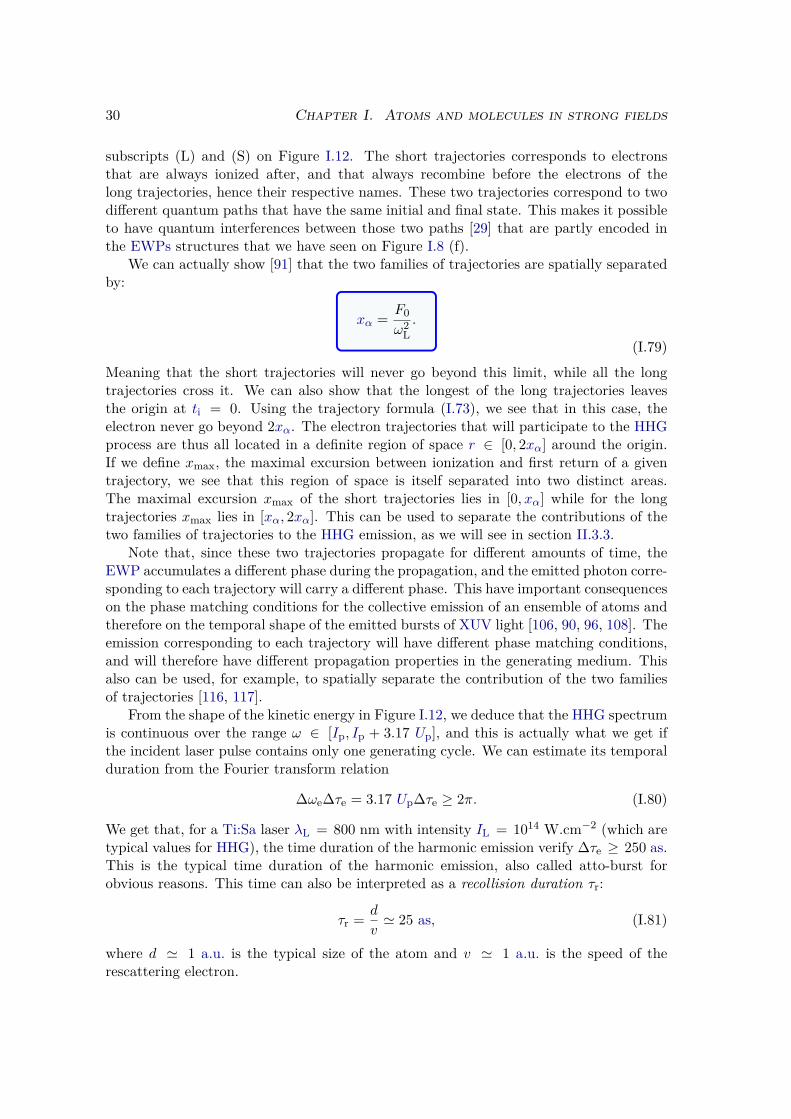
30 Chapter I. Atoms and molecules in strong fields
subscripts (L) and (S) on Figure I.12. The short trajectories corresponds to electronsthat are always ionized after, and that always recombine before the electrons of thelong trajectories, hence their respective names. These two trajectories correspond to twodifferent quantum paths that have the same initial and final state. This makes it possibleto have quantum interferences between those two paths [29] that are partly encoded inthe EWPs structures that we have seen on Figure I.8 (f).
We can actually show [91] that the two families of trajectories are spatially separatedby:
xα = F0ω2
L.
(I.79)Meaning that the short trajectories will never go beyond this limit, while all the longtrajectories cross it. We can also show that the longest of the long trajectories leavesthe origin at ti = 0. Using the trajectory formula (I.73), we see that in this case, theelectron never go beyond 2xα. The electron trajectories that will participate to the HHGprocess are thus all located in a definite region of space r ∈ [0, 2xα] around the origin.If we define xmax, the maximal excursion between ionization and first return of a giventrajectory, we see that this region of space is itself separated into two distinct areas.The maximal excursion xmax of the short trajectories lies in [0, xα] while for the longtrajectories xmax lies in [xα, 2xα]. This can be used to separate the contributions of thetwo families of trajectories to the HHG emission, as we will see in section II.3.3.
Note that, since these two trajectories propagate for different amounts of time, theEWP accumulates a different phase during the propagation, and the emitted photon corre-sponding to each trajectory will carry a different phase. This have important consequenceson the phase matching conditions for the collective emission of an ensemble of atoms andtherefore on the temporal shape of the emitted bursts of XUV light [106, 90, 96, 108]. Theemission corresponding to each trajectory will have different phase matching conditions,and will therefore have different propagation properties in the generating medium. Thisalso can be used, for example, to spatially separate the contribution of the two familiesof trajectories [116, 117].
From the shape of the kinetic energy in Figure I.12, we deduce that the HHG spectrumis continuous over the range ω ∈ [Ip, Ip + 3.17 Up], and this is actually what we get ifthe incident laser pulse contains only one generating cycle. We can estimate its temporalduration from the Fourier transform relation
∆ωe∆τe = 3.17 Up∆τe ≥ 2π. (I.80)
We get that, for a Ti:Sa laser λL = 800 nm with intensity IL = 1014 W.cm−2 (which aretypical values for HHG), the time duration of the harmonic emission verify ∆τe ≥ 250 as.This is the typical time duration of the harmonic emission, also called atto-burst forobvious reasons. This time can also be interpreted as a recollision duration τr:
τr = d
v' 25 as, (I.81)
where d ' 1 a.u. is the typical size of the atom and v ' 1 a.u. is the speed of therescattering electron.
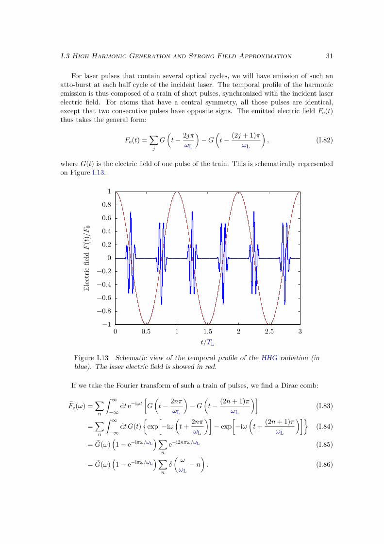
I.3 High Harmonic Generation and Strong Field Approximation 31
For laser pulses that contain several optical cycles, we will have emission of such anatto-burst at each half cycle of the incident laser. The temporal profile of the harmonicemission is thus composed of a train of short pulses, synchronized with the incident laserelectric field. For atoms that have a central symmetry, all those pulses are identical,except that two consecutive pulses have opposite signs. The emitted electric field Fe(t)thus takes the general form:
Fe(t) =∑j
G
(t− 2jπ
ωL
)−G
(t− (2j + 1)π
ωL
), (I.82)
where G(t) is the electric field of one pulse of the train. This is schematically representedon Figure I.13.
−1
−0.8
−0.6
−0.4
−0.2
0
0.2
0.4
0.6
0.8
1
0 0.5 1 1.5 2 2.5 3
Electric
fieldF
(t)/F
0
t/TL
Figure I.13 Schematic view of the temporal profile of the HHG radiation (inblue). The laser electric field is showed in red.
If we take the Fourier transform of such a train of pulses, we find a Dirac comb:
Fe(ω) =∑n
∫ ∞−∞
dt e−iωt[G
(t− 2nπ
ωL
)−G
(t− (2n+ 1)π
ωL
)](I.83)
=∑n
∫ ∞−∞
dtG(t)
exp[−iω
(t+ 2nπ
ωL
)]− exp
[−iω
(t+ (2n+ 1)π
ωL
)](I.84)
= G(ω)(1− e−iπω/ωL
)∑n
e−i2nπω/ωL (I.85)
= G(ω)(1− e−iπω/ωL
)∑n
δ
(ω
ωL− n
). (I.86)
32 Chapter I. Atoms and molecules in strong fields
This Dirac comb directly explains why we only see harmonics of the incident laser field inthe HHG spectrum. The continuous Fourier transform of one atto-burst G(ω) will act asan envelope over this Dirac comb. Moreover we see that the
(1− e−iπω/ωL
)factor vanishes
for even harmonics. This elucidates why we only see the odd harmonics of the incidentlaser field in the HHG spectrum. Of course this is strongly related to the symmetry ofthe system. In anisotropic media such as oriented or aligned molecules [98] or with otherlaser polarizations [118–121] even harmonics are observed in HHG spectra.
I.3.3 Strong field approximation
We saw that we could explain most of the features of the HHG process with the semi-classical model. We will now go a little further in our description by invoking the StrongField Approximation (SFA). This approximation allows to develop an interpretative quan-tum model for HHG: the Lewenstein model [11]. This widely used model justifies, in thequantum framework, all the results and interpretations that we just obtained with thesemi-classical model, hence its immense success.
a) Assumptions
Let us start by summarizing all the approximations of this model, keeping in mind that,of course, these approximations have limitations, as will be discussed later in this thesis.We want to solve the TDSE in the length gauge (I.21), so we first list all the assumptionswe made to obtain this Hamiltonian:
Semi-classical approximation: the atom is treated with quantum mechanics, but theEM field is classical.
Non relativistic electron: verified for IL ≤ 1016 W.cm−2, this allowed us to neglectthe influence of the magnetic field on the electron.
Dipole approximation: verified for large wavelength with respect to the atom size λL r,this allowed to neglect the r dependency in the field quantities.
To these, we add new assumptions for the description of our system:
Frozen nuclei: we drop the dependency in the position of the nuclei. This is justifiedby the large difference of masses between the electron and the nuclei. Since thenuclei are much heavier, their dynamics evolves at much longer time scales. We cantherefore neglect their motion for very short laser pulses of a few tens of fs.
Single Active Electron (SAE): the only active electron evolves under the action of aneffective potential V0 that represents its averaged interaction with the whole ioniccore.
In this framework, the SFA assumptions read [11]:
(a) The contributions of the excited bound states |ϕi〉, with i ≥ 1, are neglected. Thewave function can thus be decomposed on the ground state |ϕ0〉 and on the contin-uum states |ϕE〉 only.
I.3 High Harmonic Generation and Strong Field Approximation 33
(b) The depletion of the ground state |ϕ0〉 is neglected, the population in the groundstate is considered to be equal to one.
(c) Plane Wave Approximation (PWA): The influence of the potential V0 on theionized electron is neglected, i.e. the continuum states |ϕE〉 are approximated byplane waves |k〉, where 〈r|k〉 = eik·r. Note that we also made this approximationfor the classical analysis made in the previous section.
Assumption (a) implies that we are out of any resonance, which is generally the casefor the photon energies used in HHG. Assumption (b) is valid for intensities that arebelow the saturation intensity. Assumption (c) is systematically valid for short-rangepotentials. For Coulomb-like potential, it is justified under two conditions: when theelectron is far from the nucleus, it requires that the electric field is large enough, i.e. thatthe Keldysh parameter is small γ ≤ 1, and when the electron returns close to the nucleus,it requires that this electron has a sufficiently high kinetic energy so that it does not feelthe potential V0. This approximation will thus only hold for the high energy part of theemitted spectrum. The low energy part ωe ≤ Ip cannot be accurately computed in thismodel.
b) Dipole expression
From assumptions (a) and (c) we get the following ansatz for the wave function
|ψ(t)〉 = eiIpt(a0(t) |ϕ0〉+
∫dk c(k, t) |k〉
), (I.87)
with (p2
2 + V0(r))|k〉 ' p2
2 |k〉 = k2
2 |k〉 , (I.88)
and with assumption (b), we get a0(t) ' 1. Inserting (I.87) in the TDSE and projectingover |k〉, we get the following differential equation for the time-dependent coefficients:
c(k, t) = −i(Ip + k2
2
)c(k, t)− iFL(t)
(〈k|x |ϕ0〉+
∫dk′ c(k′, t) 〈k|x
∣∣k′⟩) , (I.89)
where we assumed that the laser field is linearly polarized along the x direction. The lastterm can be integrated by parts:
− i∫
dk′ c(k′, t) 〈k|x∣∣k′⟩ =
∫dk′ ∂c
∂px(k′, t)
⟨k∣∣k′⟩ = ∂c
∂kx(k, t). (I.90)
We define dion the ionization dipole matrix element:
dion(k, t) = FL(t) 〈k|x |ϕ0〉 , (I.91)
so that (I.89) finally reads
c(k, t) = −i(Ip + k2
2
)c(k, t)− idion(k, t) + FL(t) ∂c
∂kx(k, t). (I.92)
34 Chapter I. Atoms and molecules in strong fields
This equation integrates to:
c(k, t) =∫ t
0dt′dion(k−AL(t) + AL(t′), t′)
× exp[−i∫ t
t′dτ(
(k−AL(t) + AL(τ))2
2 + Ip
)],
(I.93)
where the vector potential AL is defined in the Coulomb gauge by (I.7).We are interested in the radiation emitted by the system, which is proportional to the
average value of the dipole operator:
D(t) = 〈ψ(t)| D |ψ(t)〉 . (I.94)
Depending on the chosen representation, D may either be the position Dd, velocity Dvor acceleration Da operator defined in (II.77). The three representations are actuallyequivalent. In fact, it is easy to show by integration by part that they are simply relatedto one another by factors of ω, see section II.3.2 for more details.
Using the approximate ansatz (I.87), we get:
D(t) = 〈ϕ0| D |ϕ0〉+∫
dk c(k, t) 〈ϕ0| D |k〉+∫
dk c∗(k, t) 〈k| D |ϕ0〉
+∫∫
dk dk′ c∗(k′, t)c(k, t)⟨k′∣∣ D |k〉 . (I.95)
We neglect the continuum-continuum contributions [11, 122], and drop the ground statecontribution since it cancels for apolar systems and only adds a constant component tothe spectrum for polar molecules. We also perform the substitution p = k−AL(t), andget
D(t) =∫ t
0dt′∫
dp drec(p + AL(t))dion(p + AL(t′), t′) e−iS(p,t,t′) +c.c., (I.96)
where drec is the recombination dipole matrix element:
drec(p) = 〈ϕ0| D |p〉 , (I.97)
and S the quasiclassical action:
S(p, t, t′) =∫ t
t′dτ(
[p + AL(τ)]2
2 + Ip
). (I.98)
We can interpret (I.96) in the same spirit as in time-dependent perturbation the-ory in section I.2.1 c): at t = 0 the system is in state |ϕ0〉, and it accumulates aphase eiIpt′ until time t′ where it is transferred to state |p〉 with transition matrix ele-ment dion(p + AL(t′), t′). Afterwards it evolves in that state under the influence of thefield only, accumulating a phase
∫ tt′ dτ [p + AL(τ)]2 /2, and it finally recombines to the
ground state |ϕ0〉 at time t with transition matrix element drec(p + AL(t)). The last eiIpt
factor comes from (I.87). It is remarkable that we recognize the three steps mentionedbefore: ionization, propagation in the continuum and recombination to the ground state.
I.3 High Harmonic Generation and Strong Field Approximation 35
To get the spectrum of the emitted radiation we need to compute the Fourier transformof the dipole:
D(ω) = D+(ω) + D−(ω), (I.99)with
D+(ω) =∫
dt∫ t
0dt′∫
dp drec(p + AL(t))dion(p + AL(t′), t′) e−i[S(p,t,t′)+ωt], (I.100)
and D−(ω) = D∗+(−ω).Note that within SFA the two gauges described in sections I.1.2 and I.1.1 are not
equivalent anymore. Here we made all the calculations in the length gauge, i.e. with theER expression of the Hamiltonian (I.21). If we make the same derivation in the velocitygauge, i.e. with the AP expression of Hamiltonian (I.14), we obtain [84]
D+(ω) =∫
dt∫ t
0dt′∫
dp drec(p)dion(p, t′) e−i[S(p,t,t′)+ωt], (I.101)
where the ionization dipole element reads:
dion(p, t′) = AL(t′)⟨
p∣∣∣∣∣−i ∂
∂px+ AL
2(t′)2
∣∣∣∣∣ϕ0
⟩. (I.102)
These differences between the results obtained in each of the two gauges can actually beused to test the validity of the SFA approximations.
c) Saddle point approximation
The triple integral (I.100) cannot be computed analytically in the general case, and itsnumerical evaluation is very costly. Nevertheless we can get an approximate, and intuitive,evaluation of it by performing the Saddle Point Approximation (SPA). Since Ip/ωL isvery large, the quasiclassical action has very large variations, and the exponential term in(I.100) oscillates very fast. If it oscillates much faster than the preexponential term, thenthe main contribution to the integral comes from the points where the phase is stationary:
∇(S(p, t, t′)± ωt
)= 0, (I.103)
where the ∇ operator contains here the derivatives with respect to all the variables of S.The sign in front of ω is a + for D+(ω) and a − for D−(ω). This evaluation of the integralrelies on the method of stationary phase [123, 124], that allows to compute the asymptoticform of generalized Fourier transform integrals. More details are given in Appendix A.
The evaluation of (I.100) in the SPA reduces to solving (I.103). For the term D−(ω)this gives ∫ t
t′[p + AL(τ)] dτ = 0
[p + AL(t)]22 + Ip − ω = 0
[p + AL(t′)]22 + Ip = 0.
(I.104a)
(I.104b)
(I.104c)
36 Chapter I. Atoms and molecules in strong fields
These three equations actually encode the three step model. The first of them involves theclassical velocity p+AL of the free electron in the laser field. The integral of this velocityis equal to the difference between the positions at recombination and at ionization [11]:∫ t
t′[p + AL(τ)] dτ = r(t)− r(t′) (I.105)
The solutions of (I.104a) are thus quantum paths where the electron is ionized at posi-tion r(t′) at time t′ and then returns to this same position a later time t. This is what weintuitively expect of an electron being ionized at the nucleus and later returning to thisnucleus to recombine.
The second equation encodes the energy conservation at the recombination time t.Indeed [p + AL]2/2 is the kinetic energy of the electron in the continuum, (I.104b) thusstates that the energy ω of the emitted photon is equal to the energy difference betweenthe electron in the continuum and the ground state. We retrieve the energy conserva-tion (I.76).
Finally, the third saddle point equation (I.104c) represents the energy conservationat ionization time t′. Note that this equation does not have any solution for real valuesof p and t′. The solutions of (I.104) thus involves complex stationary points for thephase. This is related to the intrinsic quantum nature of tunnel ionization, which has noclassical counterpart. The imaginary part of t′ may be interpreted as the tunnel ionzationtime [11]. Observe that this ionization time is the time when the electron starts itstrajectory in the continuum, but cannot be related to a tunnel ionization duration. Itis actually impossible to define such an ionization duration rigorously and without anyambiguity in the framework of quantum mechanics [125, 126].
If we compute numerically the solutions of (I.104) we find two families of solutions,which are the analogues of the short and long trajectories described in the previous section.In conclusion the quantum paths that are solutions of (I.104), i.e. the paths that give thelargest contribution to HHG, are actually the quantum equivalents of the trajectories ofthe classical three step model.
Note that for the term D+(ω) the saddle point equations (I.104) are identical, exceptfor (I.104b), where there is a change of sign in front of ω:
[p + AL(t)]22 + Ip + ω = 0. (I.106)
Since this equation does not satisfy energy conservation, the contribution of the D+(ω)term will actually be negligible in (I.99), and we will only keep D−(ω) in the following.
We note (pat, tat, t′at) the solutions of the atomic equations (I.104) to distinguish them
from the solutions of the molecular equations that we will detail in the following section.The Fourier transform of the dipole (I.100) finally writes:
Dat(ω) =∑j=S,L
C(tat(j), t
′(j)at )drec(pat
(j) + AL(tat(j)))dion(pat
(j) + AL(t′(j)at ), t′(j)at ) e−iSat ,
(I.107)where S and L stands for the short and long trajectories respectively and Sat is thequasiclassical action evaluated at the stationary point:
Sat = S(pat, tat, t′at)− ωtat (I.108)
I.3 High Harmonic Generation and Strong Field Approximation 37
The saddle point prefactor C reads [127]:
C(t, t′) =( 2π
i(t− t′)
) 32 π√
detHSp(t, t′), (I.109)
where HSp is the Hessian matrix of Sp(t, t′) = S(pat(t, t′), t, t′)−ωt, where pat(t, t′) is thesolution of (I.104a):
detHSp(t, t′) = ∂2Sp∂t2
∂2Sp∂t′2
−(∂2Sp∂t∂t′
)2
. (I.110)
d) Molecular saddle point approximation
In principle the development that we just made can be applied to atoms or molecules.Indeed the unperturbed ground state |ϕ0〉 and the ionization potential Ip that enters thefinal result (I.107) could either belong to an atom or a molecule. However in practice thisformulation gives very bad results even for the smallest molecule that comprises only twonuclei.
The reason is that the SPA that we used to compute the integral in (I.100) assumesthat the preexponential term drecdion varies slowly with respect to the quasiclassical ac-tion. For atoms this will almost always be the case and we can use (I.107). On the con-trary, in the case of molecules this preexponential factor may cancel for values of (p, t, t′)that reflects the molecular orbital structure. If this zero is close to the stationary point,i.e. the solution of (I.104), then the SPA fails to predict the correct value of the integral.We thus need to take this zero into account when looking for stationary points. Saidotherwise, we need to take the molecular structure into account in our description.
The method that we present here for homonuclear diatomic molecules has been intro-duced in [84], and then developed in [128, 129] and will be investigated in more detailsin Chapter IV. It relies on the Linear Combination of Atomic Orbitals (LCAO) approxi-mation, which adds to all the assumptions listed before in section I.3.3 a). It amounts towrite the ground state |ϕ0〉 as a sum of two shifted functions φa:
ϕ0(r) = 1√2(1 + w(R)
) [φa
(r− R
2
)+ φa
(r + R
2
)], (I.111)
where w(R) is the overlap between the two shifted φa orbitals, and R is the internuclearvector. We choose the center of the molecule as origin of the coordinate system, so thatnucleus 1 is located at −R/2 and nucleus 2 at +R/2. Inserting (I.111) in the expression
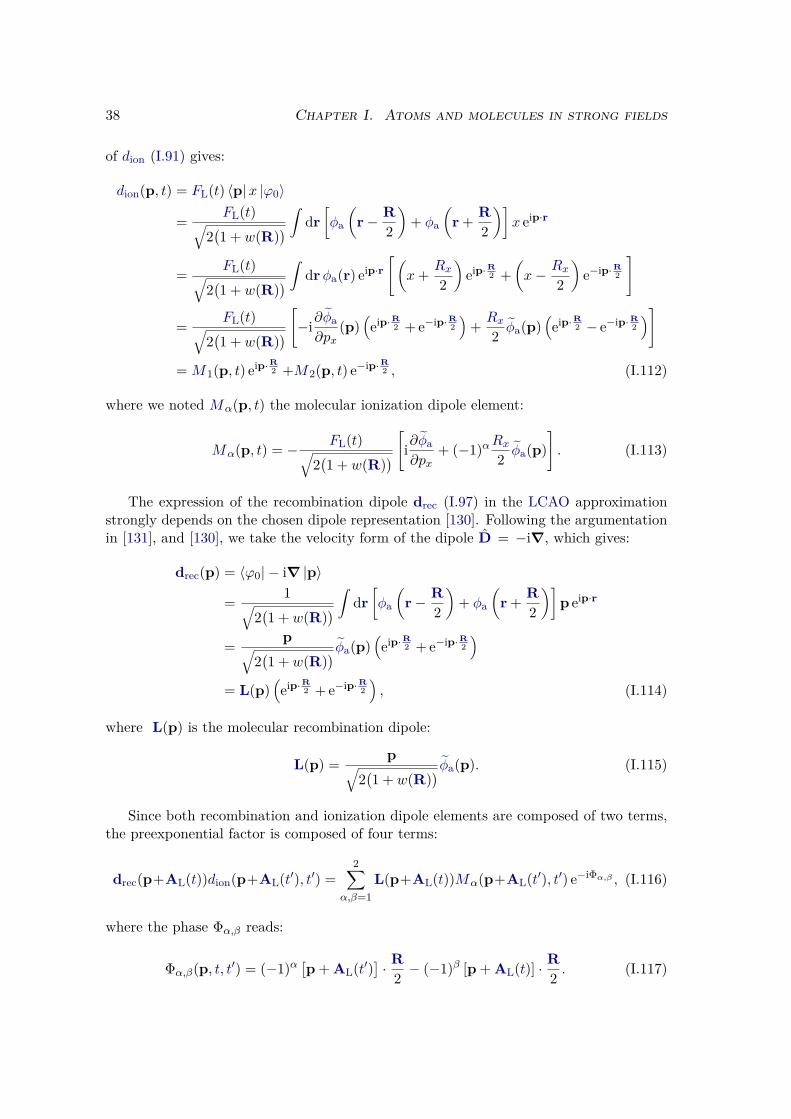
38 Chapter I. Atoms and molecules in strong fields
of dion (I.91) gives:
dion(p, t) = FL(t) 〈p|x |ϕ0〉
= FL(t)√2(1 + w(R)
) ∫ dr[φa
(r− R
2
)+ φa
(r + R
2
)]x eip·r
= FL(t)√2(1 + w(R)
) ∫ drφa(r) eip·r[(
x+ Rx2
)eip·R2 +
(x− Rx
2
)e−ip·R2
]
= FL(t)√2(1 + w(R)
)[−i∂φa∂px
(p)(eip·R2 + e−ip·R2
)+ Rx
2 φa(p)(eip·R2 − e−ip·R2
)]
= M1(p, t) eip·R2 +M2(p, t) e−ip·R2 , (I.112)
where we noted Mα(p, t) the molecular ionization dipole element:
Mα(p, t) = − FL(t)√2(1 + w(R)
)[i∂φa∂px
+ (−1)αRx2 φa(p)]. (I.113)
The expression of the recombination dipole drec (I.97) in the LCAO approximationstrongly depends on the chosen dipole representation [130]. Following the argumentationin [131], and [130], we take the velocity form of the dipole D = −i∇, which gives:
drec(p) = 〈ϕ0| − i∇ |p〉
= 1√2(1 + w(R)
) ∫ dr[φa
(r− R
2
)+ φa
(r + R
2
)]p eip·r
= p√2(1 + w(R)
) φa(p)(eip·R2 + e−ip·R2
)= L(p)
(eip·R2 + e−ip·R2
), (I.114)
where L(p) is the molecular recombination dipole:
L(p) = p√2(1 + w(R)
) φa(p). (I.115)
Since both recombination and ionization dipole elements are composed of two terms,the preexponential factor is composed of four terms:
drec(p+AL(t))dion(p+AL(t′), t′) =2∑
α,β=1L(p+AL(t))Mα(p+AL(t′), t′) e−iΦα,β , (I.116)
where the phase Φα,β reads:
Φα,β(p, t, t′) = (−1)α[p + AL(t′)
]· R
2 − (−1)β [p + AL(t)] · R2 . (I.117)
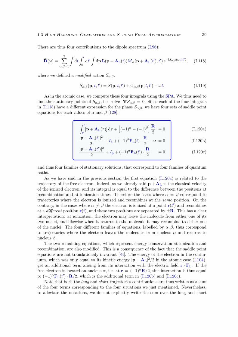
I.3 High Harmonic Generation and Strong Field Approximation 39
There are thus four contributions to the dipole spectrum (I.96):
D(ω) =2∑
α,β=1
∫dt∫ t
0dt′∫
dp L(p + AL(t))Mα(p + AL(t′), t′) e−iSα,β(p,t,t′), (I.118)
where we defined a modified action Sα,β:
Sα,β(p, t, t′) = S(p, t, t′) + Φα,β(p, t, t′)− ωt. (I.119)
As in the atomic case, we compute these four integrals using the SPA. We thus need tofind the stationary points of Sα,β, i.e. solve ∇Sα,β = 0. Since each of the four integralsin (I.118) have a different expression for the phase Sα,β, we have four sets of saddle pointequations for each values of α and β [128]:
∫ t
t′[p + AL(τ)] dτ +
[(−1)α − (−1)β
] R2 = 0
[p + AL(t)]22 + Ip + (−1)βFL(t) · R
2 − ω = 0
[p + AL(t′)]22 + Ip + (−1)αFL(t′) · R
2 = 0
(I.120a)
(I.120b)
(I.120c)
and thus four families of stationary solutions, that correspond to four families of quantumpaths.
As we have said in the previous section the first equation (I.120a) is related to thetrajectory of the free electron. Indeed, as we already said p + AL is the classical velocityof the ionized electron, and its integral is equal to the difference between the positions atrecombination and at ionization times. Therefore the cases where α = β correspond totrajectories where the electron is ionized and recombines at the same position. On thecontrary, in the cases where α 6= β the electron is ionized at a point r(t′) and recombinesat a different position r(t), and these two positions are separated by ±R. This has a clearinterpretation: at ionization, the electron may leave the molecule from either one of itstwo nuclei, and likewise when it returns to the molecule it may recombine to either oneof the nuclei. The four different families of equations, labelled by α, β, thus correspondto trajectories where the electron leaves the molecules from nucleus α and returns tonucleus β.
The two remaining equations, which represent energy conservation at ionization andrecombination, are also modified. This is a consequence of the fact that the saddle pointequations are not translationaly invariant [84]. The energy of the electron in the contin-uum, which was only equal to its kinetic energy [p + AL]2/2 in the atomic case (I.104),get an additional term arising from its interaction with the electric field r · FL. If thefree electron is located on nucleus α, i.e. at r = (−1)αR/2, this interaction is thus equalto (−1)αFL(t′) ·R/2, which is the additional term in (I.120b) and (I.120c).
Note that both the long and short trajectories contributions are thus written as a sumof the four terms corresponding to the four situations we just mentioned. Nevertheless,to alleviate the notations, we do not explicitly write the sum over the long and short

40 Chapter I. Atoms and molecules in strong fields
trajectories in the final expression of the dipole spectrum, which reads
Dα,β(ω) =2∑
α,β=1Cα,β(tαβ, t′αβ)L(pαβ + AL(tαβ))Mα(pαβ + AL(t′αβ), t′αβ) e−iSα,β , (I.121)
where (pαβ, tαβ, t′αβ) are the molecular stationary points, and Cα,β is the saddle pointprefactor (I.109).
Chapter IINumerical methods
During my PhD, I studied diverse systems with different dimensionality and complexity.For all these systems, we want to solve the same equation, namely the Schrödinger equa-tion. But in practice we use distinct methods suited to the specificity of each system andeach physical phenomenon we are interested in. All the results presented in this thesiswere computed with numerical programs written by myself, unless explicitly stated oth-erwise. In this chapter are presented the numerical methods and algorithms underlyingthese programs. In each case, we choose the numerical method as a compromise betweena reasonable computational cost, and a controllable numerical error. For the relativelysmall systems considered here, limitations usually come from the number of operationsrather than memory. We will thus define our computational cost by the complexity ofthe algorithms used in the different numerical methods.
Numerical error originates from two sources: numerical precision, and algorithm pre-cision. Indeed, since our computers have a finite memory, each number is stored on adefinite number of bytes. For example, here we use 16 bytes to store each real number,which is the so-called double precision. This defines our machine accuracy. All the numer-ical arithmetic is thus performed on truncated numbers. Consequently each arithmeticoperation is performed with a finite precision which depends on the type of operation andon the relative value of the numbers involved in the operation. In general the numericalerror is particularly important when summing two numbers that have very different or-ders of magnitude, or when subtracting two numbers that are very close. In general, it isactually quite tricky to control this numerical error. Besides, even with an infinite com-puter memory the algorithm error remains. The latter arises from both the discretizationof the Hilbert space and the discretization of time. This algorithm error can in general becontrolled by raising the number of points in each of these discretizations, until we reachwhat we call convergence i.e. the numerical machine accuracy.
The convergence properties of an algorithm are of crucial importance. A faster con-vergence allows to save some computational time and thus to describe larger or morecomplex systems. We will be highly concerned by these convergence properties, i.e. bythe numerical error made by each algorithm, in the presentation of the numerical methods.
Objectives
ü Define 1D and 2D model systems for atoms and molecules.
41
42 Chapter II. Numerical methods
ü Compute energies and stationary states of these systems numerically (TISE).
ü Compute the time-dependent wave function in presence of an EM field (TDSE).
ü Analyze the time-dependent wave function to extract physical insight, and measur-able quantities relevant for experiments.
ü In each case, find the best compromise between numerical cost and numerical error.
II.1 One dimensional systemsOne dimensional systems are perfect toy models for which we can make extensive numer-ical simulations, and thus get physical insight into intricate physical phenomena. Theyare particularly adapted to the case of tunnel ionization since the introdution of paraboliccoordinates reduces the problem of the hydrogen atom in a static electric field to a onedimensional problem [132]. They are also suited to study HHG in atoms and moleculesaligned along the electric field. This can be seen from the solution of the SFA equationsdeveloped in the previous chapter. We can show that the momentum p of the electron,which is solution of (I.104a) for atoms and of (I.120a) for aligned molecules, will actuallyalways be parallel to the laser polarization direction.
II.1.1 Definition of the systemOur one dimensional model systems are composed of an electron initially trapped in apotential well V0. For atoms, unless otherwise stated, it will always consist of a Soft-Coulomb potential [133]:
V0(x) = − Z√a2 + x2
, (II.1)
where Z is the electric charge of the nucleus, and a is the regularization parameter whichis chosen to adjust the ionization potential Ip of the atom. Our diatomic molecules aremodelled by the sum of two shifted wells:
V0(x) = − Z/2√a2
1 + (x+R/2)2− Z/2√
a22 + (x−R/2)2
, (II.2)
where R is the internuclear distance, and a1, a2 can be used to adjust the ionizationpotential Ip and the asymmetry - thus the permanent dipole moment - of the molecule.
The time-dependent wave function ψ(x, t) is represented on a one-dimensional finitespatial grid defined by Nx points separated by a constant step ∆x going from −L to+L. It is stored as the vector (ψ(xi, t))i=1,Nx whose components are the values ψ takesat each grid point. We choose the boundary conditions so that the wave function cancelsat the border of the box ψ(−L) = ψ(L) = 0. The potential V0(x) is diagonal inthis representation. The momentum and Laplace operators are calculated by the centraldifference formulas, involving errors proportional to ∆x2:
dfdx (x) = f(x+ ∆x)− f(x−∆x)
2∆x +O(∆x2
)(II.3a)
d2f
dx2 (x) = f(x+ ∆x) + f(x−∆x)− 2f(x)∆x2 +O
(∆x2
), (II.3b)
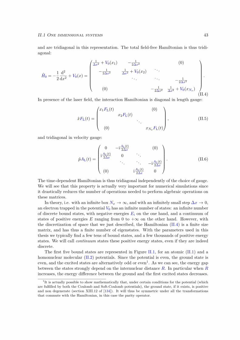
II.1 One dimensional systems 43
and are tridiagonal in this representation. The total field-free Hamiltonian is thus tridi-agonal:
H0 = −12
d2
dx2 + V0(x) =
1∆x2 + V0(x1) − 1
2∆x2 (0)
− 12∆x2
1∆x2 + V0(x2) . . .
. . . . . . − 12∆x2
(0) − 12∆x2
1∆x2 + V0(xNx)
.
(II.4)In presence of the laser field, the interaction Hamiltonian is diagonal in length gauge:
xFL(t) =
x1FL(t) (0)
x2FL(t). . .
(0) xNxFL(t)
, (II.5)
and tridiagonal in velocity gauge:
pAL(t) =
0 −iAL(t)
2∆x (0)iAL(t)
2∆x 0 . . .. . . . . . −iAL(t)
2∆x
(0) iAL(t)2∆x 0
. (II.6)
The time-dependent Hamiltonian is thus tridiagonal independently of the choice of gauge.We will see that this property is actually very important for numerical simulations sinceit drastically reduces the number of operations needed to perform algebraic operations onthese matrices.
In theory, i.e. with an infinite box Nx → ∞, and with an infinitely small step ∆x → 0,an electron trapped in the potential V0 has an infinite number of states: an infinite numberof discrete bound states, with negative energies Ei on the one hand, and a continuum ofstates of positive energies E ranging from 0 to +∞ on the other hand. However, withthe discretization of space that we just described, the Hamiltonian (II.4) is a finite sizematrix, and has thus a finite number of eigenstates. With the parameters used in thisthesis we typically find a few tens of bound states, and a few thousands of positive energystates. We will call continuum states these positive energy states, even if they are indeeddiscrete.
The first five bound states are represented in Figure II.1, for an atomic (II.1) and ahomonuclear molecular (II.2) potentials. Since the potential is even, the ground state iseven, and the excited states are alternatively odd or even1. As we can see, the energy gapbetween the states strongly depend on the internuclear distance R. In particular when Rincreases, the energy difference between the ground and the first excited states decreases.
1It is actually possible to show mathematically that, under certain conditions for the potential (whichare fulfilled by both the Coulomb and Soft-Coulomb potentials), the ground state, if it exists, is positiveand non degenerate (section XIII.12 of [134]). It will thus be symmetric under all the transformationsthat commute with the Hamiltonian, in this case the parity operator.
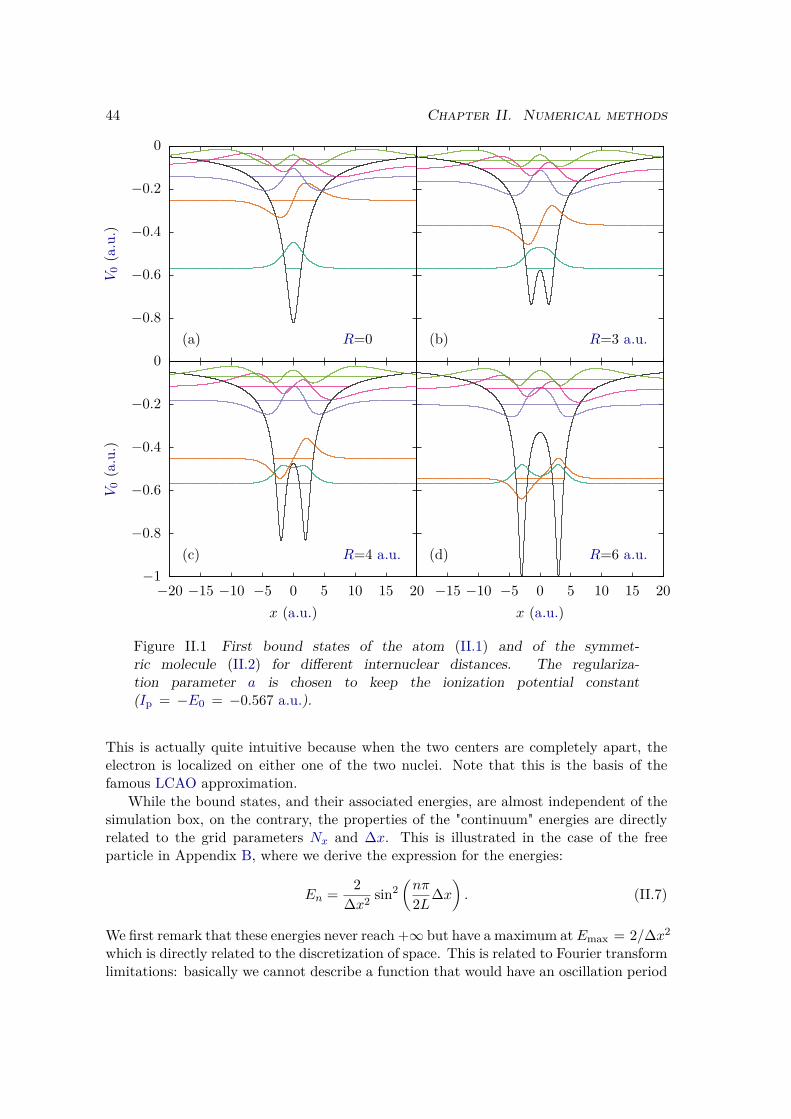
44 Chapter II. Numerical methods
−0.8
−0.6
−0.4
−0.2
0
(a) R=0 (b) R=3 a.u.
−1
−0.8
−0.6
−0.4
−0.2
0
−20 −15 −10 −5 0 5 10 15 20
(c) R=4 a.u.
−15 −10 −5 0 5 10 15 20
(d) R=6 a.u.
V0(a.u.)
V0(a.u.)
x (a.u.) x (a.u.)
Figure II.1 First bound states of the atom (II.1) and of the symmet-ric molecule (II.2) for different internuclear distances. The regulariza-tion parameter a is chosen to keep the ionization potential constant(Ip = −E0 = −0.567 a.u.).
This is actually quite intuitive because when the two centers are completely apart, theelectron is localized on either one of the two nuclei. Note that this is the basis of thefamous LCAO approximation.
While the bound states, and their associated energies, are almost independent of thesimulation box, on the contrary, the properties of the "continuum" energies are directlyrelated to the grid parameters Nx and ∆x. This is illustrated in the case of the freeparticle in Appendix B, where we derive the expression for the energies:
En = 2∆x2 sin2
(nπ
2L∆x). (II.7)
We first remark that these energies never reach +∞ but have a maximum at Emax = 2/∆x2
which is directly related to the discretization of space. This is related to Fourier transformlimitations: basically we cannot describe a function that would have an oscillation period
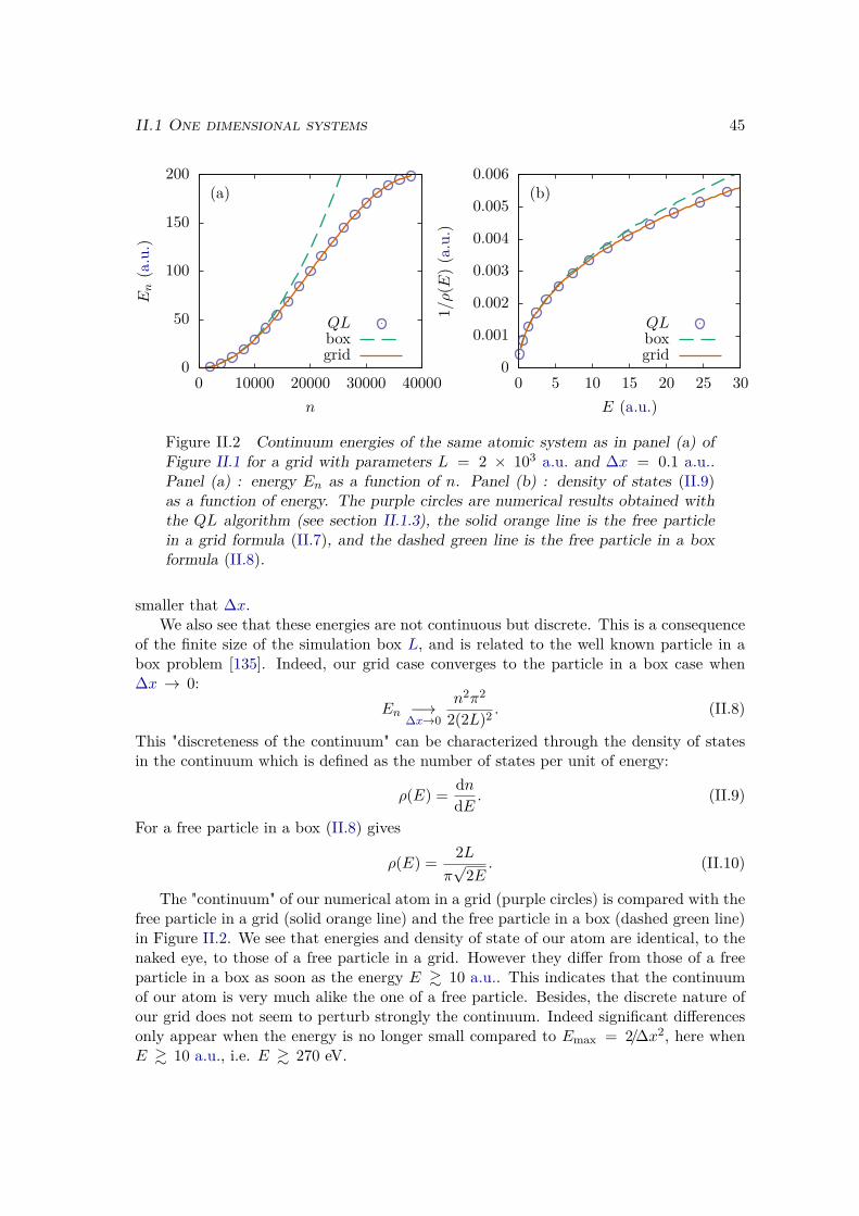
II.1 One dimensional systems 45
0
50
100
150
200
0 10000 20000 30000 40000
(a)
0
0.001
0.002
0.003
0.004
0.005
0.006
0 5 10 15 20 25 30
(b)
En(a.u.)
n
QLboxgrid
1/ρ(E
)(a.u.)
E (a.u.)
QLboxgrid
Figure II.2 Continuum energies of the same atomic system as in panel (a) ofFigure II.1 for a grid with parameters L = 2 × 10³ a.u. and ∆x = 0.1 a.u..Panel (a) : energy En as a function of n. Panel (b) : density of states (II.9)as a function of energy. The purple circles are numerical results obtained withthe QL algorithm (see section II.1.3), the solid orange line is the free particlein a grid formula (II.7), and the dashed green line is the free particle in a boxformula (II.8).
smaller that ∆x.We also see that these energies are not continuous but discrete. This is a consequence
of the finite size of the simulation box L, and is related to the well known particle in abox problem [135]. Indeed, our grid case converges to the particle in a box case when∆x → 0:
En −→∆x→0
n2π2
2(2L)2 . (II.8)
This "discreteness of the continuum" can be characterized through the density of statesin the continuum which is defined as the number of states per unit of energy:
ρ(E) = dndE . (II.9)
For a free particle in a box (II.8) gives
ρ(E) = 2Lπ√
2E. (II.10)
The "continuum" of our numerical atom in a grid (purple circles) is compared with thefree particle in a grid (solid orange line) and the free particle in a box (dashed green line)in Figure II.2. We see that energies and density of state of our atom are identical, to thenaked eye, to those of a free particle in a grid. However they differ from those of a freeparticle in a box as soon as the energy E & 10 a.u.. This indicates that the continuumof our atom is very much alike the one of a free particle. Besides, the discrete nature ofour grid does not seem to perturb strongly the continuum. Indeed significant differencesonly appear when the energy is no longer small compared to Emax = 2/∆x2, here whenE & 10 a.u., i.e. E & 270 eV.
46 Chapter II. Numerical methods
II.1.2 Solution of the time-dependent Schrödinger equation
a) Time discretization
The solution of the TDSE (I.3), starting from an initial state |ψ(t0)〉 at time t = t0, canbe expressed as
|ψ(t)〉 = exp[−i∫ t
t0H(τ) dτ
]|ψ(t0)〉 . (II.11)
Therefore if one can compute the evolution operator U(t, t+ ∆t):
U(t, t+ ∆t) = exp[−i∫ t+∆t
tH(τ) dτ
], (II.12)
then one can get the wave function at any time t > t0. This turns out to be quite a task.Firstly because the integral of the Hamiltonian cannot, in general, be computed analyti-cally. And second, because computing the exponential of a matrix is in general equivalentto diagonalize this matrix, which requires a large number of numerical operations. Tocircumvent the first problem, the most widespread technique relies on the discretizationof time. If the two limits of the integral are close enough, i.e. if ∆t is small enough, theevolution operator may be approximated as
U(t, t+ ∆t) = exp[−iH
(t+ ∆t
2
)∆t+O
(∆t3
)]. (II.13)
Note that H is evaluated at the middle of the integration interval. This is crucial to getan error that is proportional to ∆t3 rather that ∆t2, and thus to get a faster convergence.This is a general feature of the approximation of integrals, and can easily be seen fromthe Taylor expansion of the integrand:
∫ a+ε
af(x) dx =
∫ a+ε
adx[f(a) + (x− a)f ′(a) +O
((x− a)2
)](II.14)
= f(a)ε+ f ′(a)2 ε2 +O
(ε3)
(II.15)
= f(a)ε+O(ε2). (II.16)
In (II.14) we have expanded the integrand around one of the limits of the integral, and gotan error proportional to the square of the integration interval width ε2 (II.16). However,if we expand around the middle of the integration interval, the odd terms of the expansion
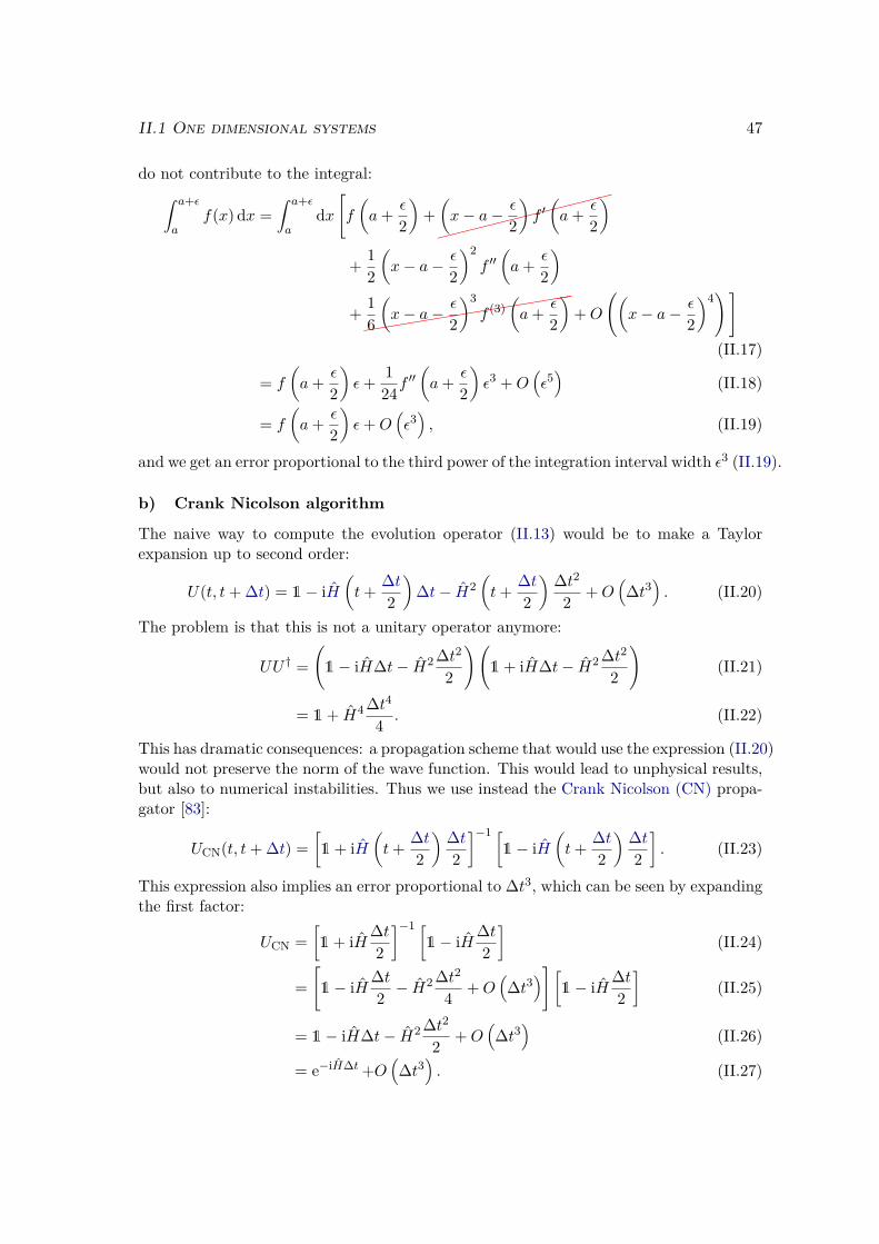
II.1 One dimensional systems 47
do not contribute to the integral:∫ a+ε
af(x) dx =
∫ a+ε
adx[f
(a+ ε
2
)+
(x− a− ε
2
)f ′(a+ ε
2
)
+ 12
(x− a− ε
2
)2f ′′(a+ ε
2
)
+((((
(((((((
((((16
(x− a− ε
2
)3f (3)
(a+ ε
2
)+O
((x− a− ε
2
)4)](II.17)
= f
(a+ ε
2
)ε+ 1
24f′′(a+ ε
2
)ε3 +O
(ε5)
(II.18)
= f
(a+ ε
2
)ε+O
(ε3), (II.19)
and we get an error proportional to the third power of the integration interval width ε3 (II.19).
b) Crank Nicolson algorithm
The naive way to compute the evolution operator (II.13) would be to make a Taylorexpansion up to second order:
U(t, t+ ∆t) = 1− iH(t+ ∆t
2
)∆t− H2
(t+ ∆t
2
) ∆t22 +O
(∆t3
). (II.20)
The problem is that this is not a unitary operator anymore:
UU † =(1− iH∆t− H2 ∆t2
2
)(1 + iH∆t− H2 ∆t2
2
)(II.21)
= 1+ H4 ∆t44 . (II.22)
This has dramatic consequences: a propagation scheme that would use the expression (II.20)would not preserve the norm of the wave function. This would lead to unphysical results,but also to numerical instabilities. Thus we use instead the Crank Nicolson (CN) propa-gator [83]:
UCN(t, t+ ∆t) =[1 + iH
(t+ ∆t
2
) ∆t2
]−1 [1− iH
(t+ ∆t
2
) ∆t2
]. (II.23)
This expression also implies an error proportional to ∆t3, which can be seen by expandingthe first factor:
UCN =[1 + iH∆t
2
]−1 [1− iH∆t
2
](II.24)
=[1− iH∆t
2 − H2 ∆t2
4 +O(∆t3
)] [1− iH∆t
2
](II.25)
= 1− iH∆t− H2 ∆t22 +O
(∆t3
)(II.26)
= e−iH∆t +O(∆t3
). (II.27)
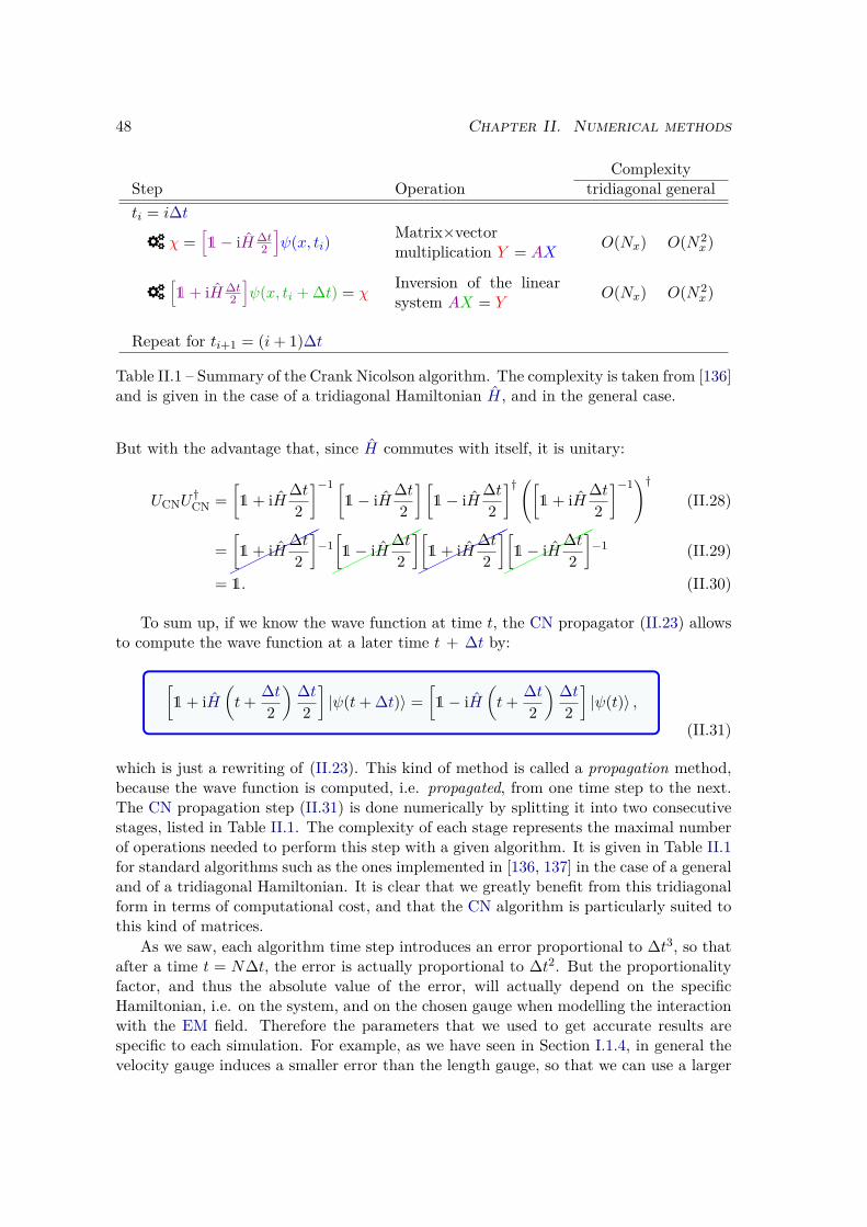
48 Chapter II. Numerical methods
ComplexityStep Operation tridiagonal generalti = i∆t
3 χ =[1− iH∆t
2
]ψ(x, ti)
Matrix×vectormultiplication Y = AX
O(Nx) O(N2x)
3[1+ iH∆t
2
]ψ(x, ti + ∆t) = χ
Inversion of the linearsystem AX = Y
O(Nx) O(N2x)
Repeat for ti+1 = (i+ 1)∆t
Table II.1 – Summary of the Crank Nicolson algorithm. The complexity is taken from [136]and is given in the case of a tridiagonal Hamiltonian H, and in the general case.
But with the advantage that, since H commutes with itself, it is unitary:
UCNU†CN =
[1 + iH∆t
2
]−1 [1− iH∆t
2
] [1− iH∆t
2
]†([1 + iH∆t
2
]−1)†(II.28)
=
[
1 + iH∆t2
]−1
[
1− iH∆t2
]
[
1 + iH∆t2
]
[
1− iH∆t2
]−1 (II.29)
= 1. (II.30)
To sum up, if we know the wave function at time t, the CN propagator (II.23) allowsto compute the wave function at a later time t + ∆t by:
[1 + iH
(t+ ∆t
2
) ∆t2
]|ψ(t+ ∆t)〉 =
[1− iH
(t+ ∆t
2
) ∆t2
]|ψ(t)〉 ,
(II.31)
which is just a rewriting of (II.23). This kind of method is called a propagation method,because the wave function is computed, i.e. propagated, from one time step to the next.The CN propagation step (II.31) is done numerically by splitting it into two consecutivestages, listed in Table II.1. The complexity of each stage represents the maximal numberof operations needed to perform this step with a given algorithm. It is given in Table II.1for standard algorithms such as the ones implemented in [136, 137] in the case of a generaland of a tridiagonal Hamiltonian. It is clear that we greatly benefit from this tridiagonalform in terms of computational cost, and that the CN algorithm is particularly suited tothis kind of matrices.
As we saw, each algorithm time step introduces an error proportional to ∆t3, so thatafter a time t = N∆t, the error is actually proportional to ∆t2. But the proportionalityfactor, and thus the absolute value of the error, will actually depend on the specificHamiltonian, i.e. on the system, and on the chosen gauge when modelling the interactionwith the EM field. Therefore the parameters that we used to get accurate results arespecific to each simulation. For example, as we have seen in Section I.1.4, in general thevelocity gauge induces a smaller error than the length gauge, so that we can use a larger
II.1 One dimensional systems 49
value of ∆t in the former than in the latter. Each calculation has thus to be meticulouslyand individually checked for convergence with respect to all simulation parameters.
In this thesis we always choose the initial state of the propagation to be the groundstate of our system. As we said in Chapter I, we will concentrate on the gas phase. Inmost experiments, the emitting system consists of supersonic gas jets [138]. The atomsand molecules in those jets are actually very cold, and a large majority of them are in theelectronic and vibrational ground state. Besides, the ground state and more generally alleigenstates, of the Hamiltonian are very useful for the subsequent analysis of the numericalresults. We will see in the next section how to compute these eigenstates.
c) Absorbing boundary conditions
In some cases, e.g. for large values of the ponderomotive potential Up, the laser electricfield may ionize the system, and create some highly energetic free electrons. Dependingon the time duration of the laser pulse, those electrons may actually travel very far fromthe nuclei during the propagation. In those cases, a very large simulation box is a priorineeded, otherwise those electrons would hit the boundaries of the box, artificially reflecton these boundaries and pollute the propagation. However, it may happen that we donot really need those electrons to describe the physical process of interest. For exampleif we are only interested in the time-dependent populations in the bound states of thesystem, then the part of the wave function that leaves the nuclei, and never return, is notparticularly relevant. Indeed we saw in Figure II.1 that the bound states of the systemare localized close to the nuclei. So all the information that is required to compute thesepopulations is contained in a very small part of the wave function. Alternatively if weare interested in HHG, then we saw in section I.3.2 that some of the ionized electrontrajectories leave the nuclei and never return, hence never participate in HHG. We alsosaw that the trajectories that return to the nuclei never go beyond the limit 2xα, so thatthe part of the wave function that lies after this limit is unnecessary for the simulation ofHHG.
We would like to reduce the size of the simulation box to the bare minimum, andthus decrease our computational cost, without inducing spurious unphysical reflexions atthe boundaries of the box. To do this we use absorbing boundary conditions. Thereare several ways to implement such an absorber [139–142]. Among them we choose anabsorbing mask [143], which consists in multiplying the wave function at each time stepby the mask function:
fabs =
= 1 if |x| ≤ L− habs
= cosζ( |x| − L+ habs
2habsπ
)if L− habs ≤|x| ≤ L
, (II.32)
where the width habs and the exponent ζ of the absorber are optimized for each propa-gation. Note that the optimization of the exponent ζ is strongly related to the value ofthe time step ∆t. Indeed a simulation with a ∆t twice smaller requires a ζ twice smallerto reach the same absorbing conditions.
50 Chapter II. Numerical methods
II.1.3 Computations of eigenstates
a) Energies
The energies and eigenstates of our field-free Hamiltonian H0 are important quantities.We use them for example to determine the initial state of our propagation, to analyze ourwave function by computing the population in the bound states, to understand qualita-tively our results, or to make analytical derivations.
Since the Hamiltonian of our system cannot be diagonalized analytically, we have todo it numerically. Our field-free Hamiltonian is real, so we compute its eigenvalues withthe QL algorithm implemented by [137] (see [144] for the mathematical description of thealgorithm, and proof of its convergence). It relies on the QL decomposition that can bedone for any real matrix A:
A = QL, (II.33)
where Q is an orthogonal matrix, and L is a lower triangular matrix. For our Nx × Nx
symmetric tridiagonal Hamiltonian, this decomposition has a complexity of O(Nx), andneeds to be done typically a few times for each of its Nx eigenvalues, resulting in a globalcomplexity of O(N2
x). This is reasonable, as long as Nx . 104, since it only has to bedone once before the propagation itself.
b) Bound eigenstates
The QL algorithm can also be used to compute the eigenvectors of a matrix, but witha complexity of O(N3
x), which is in general prohibitive. Besides we do not necessarilyneed all the eigenvectors, the ground and a few excited states are sufficent for most of thecases treated in this thesis. We thus use a much more efficient algorithm called inverseiteration [144, 137]. We make an initial guess for an eigenvalue ε0, for example using theresult of the above mentioned QL algorithm, and for the associated eigenvector y0, thenwe inverse the system (II.34a) to get w0. The vector w0 is normalized (II.34b) to get y1,and we iterate these two steps (II.34):
(A− ε0)wk = yk (II.34a)
yk+1 = wk√wk ·wk(II.34b)
If the initial guess ε0 is sufficiently close to an eigenvalue λ of A, then yk will converge tothe corresponding eigenvector in a few steps. As ε0 differed from the exact eigenvalue λ,we can use yk, which is an improved approximation of the exact eigenvector, to computea new and better guess for the eigenvalue:
εi+1 = εi + 1wki · yki
. (II.35)
Once the vector yk has converged to an eigenvector y of the Hamiltonian, it is thenrenormalized with the L2 norm to get the eigenstates |ϕ〉:
|ϕ〉 = y√∑j |y(j)|2∆x
, (II.36)
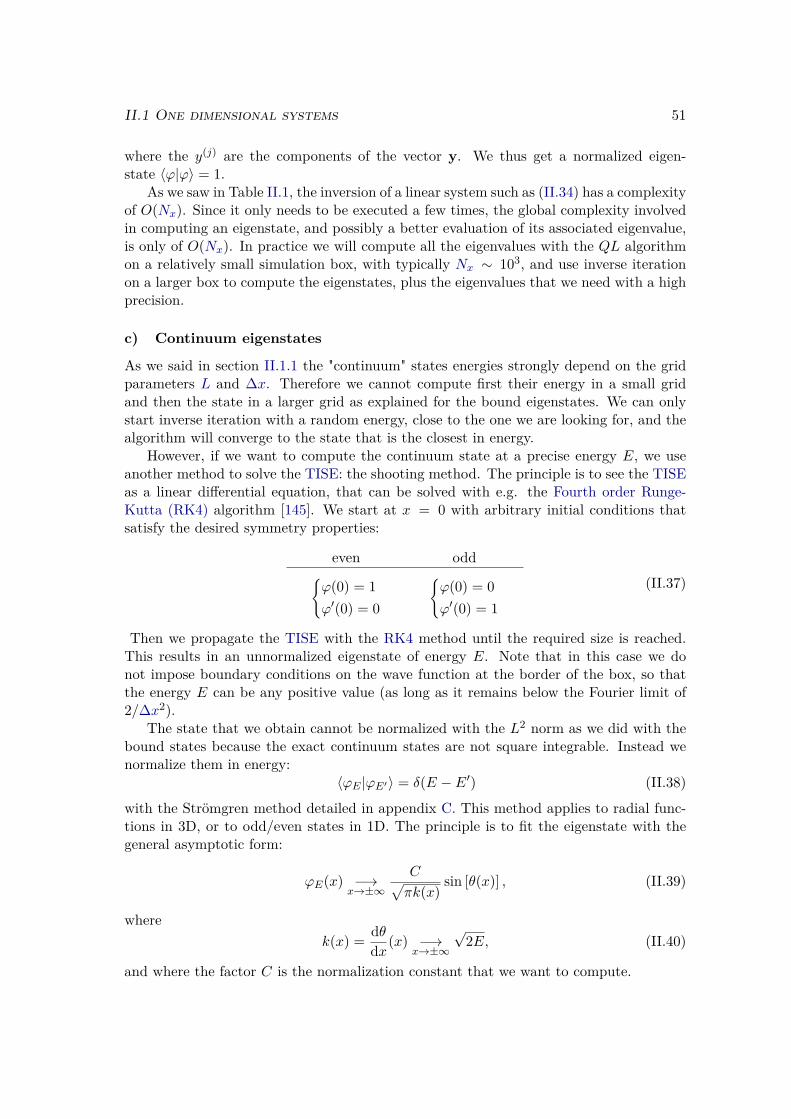
II.1 One dimensional systems 51
where the y(j) are the components of the vector y. We thus get a normalized eigen-state 〈ϕ|ϕ〉 = 1.
As we saw in Table II.1, the inversion of a linear system such as (II.34) has a complexityof O(Nx). Since it only needs to be executed a few times, the global complexity involvedin computing an eigenstate, and possibly a better evaluation of its associated eigenvalue,is only of O(Nx). In practice we will compute all the eigenvalues with the QL algorithmon a relatively small simulation box, with typically Nx ∼ 103, and use inverse iterationon a larger box to compute the eigenstates, plus the eigenvalues that we need with a highprecision.
c) Continuum eigenstates
As we said in section II.1.1 the "continuum" states energies strongly depend on the gridparameters L and ∆x. Therefore we cannot compute first their energy in a small gridand then the state in a larger grid as explained for the bound eigenstates. We can onlystart inverse iteration with a random energy, close to the one we are looking for, and thealgorithm will converge to the state that is the closest in energy.
However, if we want to compute the continuum state at a precise energy E, we useanother method to solve the TISE: the shooting method. The principle is to see the TISEas a linear differential equation, that can be solved with e.g. the Fourth order Runge-Kutta (RK4) algorithm [145]. We start at x = 0 with arbitrary initial conditions thatsatisfy the desired symmetry properties:
even oddϕ(0) = 1ϕ′(0) = 0
ϕ(0) = 0ϕ′(0) = 1
(II.37)
Then we propagate the TISE with the RK4 method until the required size is reached.This results in an unnormalized eigenstate of energy E. Note that in this case we donot impose boundary conditions on the wave function at the border of the box, so thatthe energy E can be any positive value (as long as it remains below the Fourier limit of2/∆x2).
The state that we obtain cannot be normalized with the L2 norm as we did with thebound states because the exact continuum states are not square integrable. Instead wenormalize them in energy:
〈ϕE |ϕE′〉 = δ(E − E′) (II.38)
with the Strömgren method detailed in appendix C. This method applies to radial func-tions in 3D, or to odd/even states in 1D. The principle is to fit the eigenstate with thegeneral asymptotic form:
ϕE(x) −→x→±∞
C√πk(x)
sin [θ(x)] , (II.39)
wherek(x) = dθ
dx(x) −→x→±∞
√2E, (II.40)
and where the factor C is the normalization constant that we want to compute.
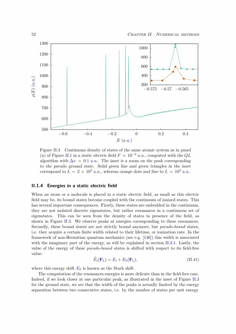
52 Chapter II. Numerical methods
500
600
700
800
900
1000
1100
1200
1300
−0.6 −0.4 −0.2 0 0.2 0.4
200
400
600
800
1000
−0.575 −0.57 −0.565
ρ(E
)(a.u.)
E (a.u.)
Figure II.3 Continuum density of states of the same atomic system as in panel(a) of Figure II.1 in a static electric field F = 10−3 a.u., computed with the QLalgorithm with ∆x = 0.1 a.u.. The inset is a zoom on the peak correspondingto the pseudo ground state. Solid green line and green triangles in the insetcorrespond to L = 2 × 10³ a.u., whereas orange dots and line to L = 103 a.u..
II.1.4 Energies in a static electric field
When an atom or a molecule is placed in a static electric field, as small as this electricfield may be, its bound states become coupled with the continuum of ionized states. Thishas several important consequences. Firstly, these states are embedded in the continuum,they are not isolated discrete eigenstates, but rather resonances in a continuous set ofeigenstates. This can be seen from the density of states in presence of the field, asshown in Figure II.3. We observe peaks at energies corresponding to these resonances.Secondly, these bound states are not strictly bound anymore, but pseudo-bound states,i.e. they acquire a certain finite width related to their lifetime, or ionization rate. In theframework of non-Hermitian quantum mechanics (see e.g. [146]) this width is associatedwith the imaginary part of the energy, as will be explained in section II.3.1. Lastly, thevalue of the energy of these pseudo-bound states is shifted with respect to its field-freevalue:
Ei(FL) = Ei + ES(FL), (II.41)
where this energy shift ES is known as the Stark shift.The computation of the resonances energies is more delicate than in the field-free case.
Indeed, if we look closer at one particular peak, as illustrated in the inset of Figure II.3for the ground state, we see that the width of the peaks is actually limited by the energyseparation between two consecutive states, i.e. by the number of states per unit energy.
II.2 Two dimensional systems 53
And we saw in section II.1.1 that this density of states is actually related to the lengthL of the simulation box. To compute the energy of the resonance with a high precision,we need to have a small energy separation with respect to the resonance natural width.Depending on the value of the electric field, this may require a very large simulation box,and thus be prohibitive. For example, with a box of size L = 2× 10³ a.u. (green trianglesin the inset of Figure II.3), we see that we only get a precision of ∼ 1% on the energy ofthe resonance.
To overcome this limitation we use the "Rbox method", developped in [147]. It relieson the fact that the energy of a particular "continuum" state depends on the size of thebox, unless it is resonant with a pseudo bound state. To illustrate this, we diagonalize theHamiltonian for various box sizes L, and then plot the energy of the "continuum" statesas a function of L on Figure II.4 for different field values. We indeed remark that theenergy of a particular state depends almost linearly on the box size L. However whenit reaches the energy E0 of the resonance, the energy is then almost constant, until itcrosses another "continuum" state. The two states do not actually cross, but have anavoided crossing, as becomes more visible for increasing values of the electric field. Wededuce the energy of the resonance from the energy of the state at the inflexion point,i.e. where its second derivative changes sign.
We see on Figure II.5 that each "continuum" state has an avoided crossing with everypseudo bound state, so that we can deduce all resonance energies from one Rbox calcu-lation. We mention that the width of the resonance can also be extracted from the Rboxmethod [148, 149], however we did not implement this feature, and prefered to rely onthe numerical solution of the TDSE (see section II.3.1).
II.2 Two dimensional systems
II.2.1 Different kinds of 2D systemsTwo dimensional systems are toy models in the same spirit as 1D systems, with relativelylow computational cost, albeit much more flexible and potentially accounting for a widervariety of physical processes. They are thus highly valuable for the development of in-terpretative analytical models. We use two dimensional grids to describe such systems,where the two dimensions do not necessarily correspond to space coordinates of the elec-tron, but may represent different variables. In this thesis we use three different kinds of2D grids:
1 electron - 2 space dimensions :In this case the two dimensions represent the position of the electron (x, y). Thesystem is composed of one electron trapped in a two dimensional Soft-Coulombpotential well, which is a simple generalization of the 1D case. For atoms it reads
V2D(r) = − Z√a2 + r2
, (II.42)
and for diatomic molecules:
V2D(r) = − Z/2√a2
1 + (r + R/2)2− Z/2√
a22 + (r−R/2)2
. (II.43)
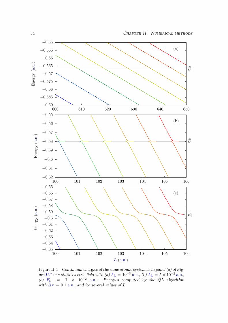
54 Chapter II. Numerical methods
−0.59
−0.585
−0.58
−0.575
−0.57
−0.565
−0.56
−0.555
−0.55
600 610 620 630 640 650
(a)
E0
−0.62
−0.61
−0.6
−0.59
−0.58
−0.57
−0.56
−0.55
100 101 102 103 104 105 106
(b)
E0
−0.65−0.64−0.63−0.62−0.61−0.6−0.59−0.58−0.57−0.56−0.55
100 101 102 103 104 105 106
(c)
E0
Energy
(a.u.)
Energy
(a.u.)
Energy
(a.u.)
L (a.u.)
Figure II.4 Continuum energies of the same atomic system as in panel (a) of Fig-ure II.1 in a static electric field with (a) FL = 10−3 a.u., (b) FL = 5× 10⁻² a.u.,(c) FL = 7 × 10⁻² a.u.. Energies computed by the QL algorithmwith ∆x = 0.1 a.u., and for several values of L.
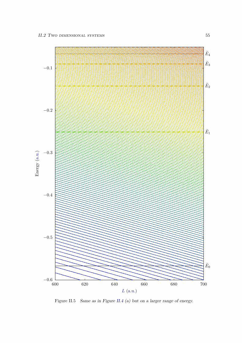
II.2 Two dimensional systems 55
−0.6
−0.5
−0.4
−0.3
−0.2
−0.1
600 620 640 660 680 700
E0
E1
E2
E3
E4
Energy
(a.u.)
L (a.u.)
Figure II.5 Same as in Figure II.4 (a) but on a larger range of energy.
56 Chapter II. Numerical methods
The field-free Hamiltonian is very similar to the 1D case:
H2D = −12∂2
∂x2 −12∂2
∂y2 + V2D(r). (II.44)
This system allows e.g. to study diatomic molecules that can have different orien-tations with respect to the laser polarization.
2 electrons - 1 space dimension each :In this case, the two dimensions are the positions of two electrons (x1, x2), that aretrapped in a one dimensional Soft-Coulomb potential well, which is defined in (II.1)and (II.2). An additional term in the Hamiltonian accounts for the inter-electronicrepulsion:
Vee(x1, x2) = 1√b2 + (x1 − x2)2
. (II.45)
The field-free Hamiltonian thus reads
H2E = −12∂2
∂x21− 1
2∂2
∂x22
+ V0(x1) + V0(x2) + Vee(x1, x2). (II.46)
This systems is a very simple model to study electron correlations.
1 nucleus and 1 electron - 1 space dimension each :This system is composed of two nuclei and a one dimensional electron. The twodimensions are the position of the electron and the internuclear distance (x,R).Compared to the 1D case, the Hamiltonian have two additional terms : one for thekinetic energy of the nuclei and another for the internuclear repulsion2 VNN. Notethat the internuclear distance R that appeared in the electron-nucleus interactionpotential is now a variable, instead of a parameter. The Hamiltonian thus reads
HXR = − 12µ
∂2
∂R2 + VNN(R)− 12∂2
∂x2 + V0(R, x), (II.47)
where
V0(R, x) = − Z√a1(R)2 + (x+R/2)2
− Z√a2(R)2 + (x−R/2)2
. (II.48)
The parameters a1 and a2 are adjusted so that the electronic potential energy surfaceof the ground state reproduces the one of the system we want to model, e.g. the H2molecule.
This is a simple model that allows to go beyond the Born-Oppenheimer (BO) ap-proximation, and investigate vibronic dynamics in molecules.
2In general, the latter is adjusted on the ionic potential energy surface of interest.
II.2 Two dimensional systems 57
II.2.2 Split-operator methodFor the three 2D systems just described the Hamiltonian is sparse, i.e. it has a largenumber of matrix elements that are zero, but is not tridiagonal. The CN algorithm forpropagation that we described in section II.1.2 b) is not adapted to this case: it involvessteps with a complexity of O(N2), while we had a complexity of O(N) in the tridiagonalcase. Note that N is here the total size of the 2D grid, and is in general much largerthan the size Nx of the 1D grid. We can do better than this O(N2) complexity byusing another propagation scheme: the split operator algorithm. This scheme relies ona decomposition of the Hamiltonian into two terms: a kinetic energy term T diagonal inthe p representation, and a potential energy term V diagonal in the r representation. Itis therefore tempting to apply each of these terms separately, interspersed with simplechanges of representation. However T and V do not commute:[
V , T]6= 0, (II.49)
so, if we simply decompose the evolution operator:
e−iH∆t = e−i(T+V )∆t ' e−iT∆t e−iV∆t, (II.50)
we get an error proportional to ∆t2 (see appendix D). Instead the split operator methoduses the decomposition
e−i(T+V )∆t = e−iV∆t/2 e−iT∆t e−iV∆t/2 +O(∆t3
), (II.51)
with an error proportional to ∆t3, as shown in appendix D.To sum up, the split-operator propagation scheme can be written as
|ψ(t+ ∆t)〉 = e−iV∆t/2 e−iT∆t e−iV∆t/2 |ψ(t)〉 ,(II.52)
where the potential V is diagonal in the r representation:
e−iV∆t/2 ψ(x1, x2, t) = e−iV (x1,x2)∆t/2 ψ(x1, x2, t), (II.53)
and the kinetic energy T is diagonal in the p representation:
e−iT∆t ψ(p1, p2, t) = e−ip21
2µ1−i
p222µ2 ψ(p1, p2, t), (II.54)
where x1 and x2 are generic names for the two dimensions of the grid, and p1 and p2are the associated momenta. The r and p representations are related through a Fouriertransform, which can be computed efficiently with the FFT algorithm, implemented inthe Fastest Fourier Transform in the West (FFTW) library [150]. The complexity of theFFT depends on the size of the matrix, and more precisely on its prime decomposition.In general it is of the form O(N logN), which is much better that O(N2). One step of thesplit-operator algorithm is summarized in Table II.2. We see that its overall complexityis limited by the Fourier transform steps.
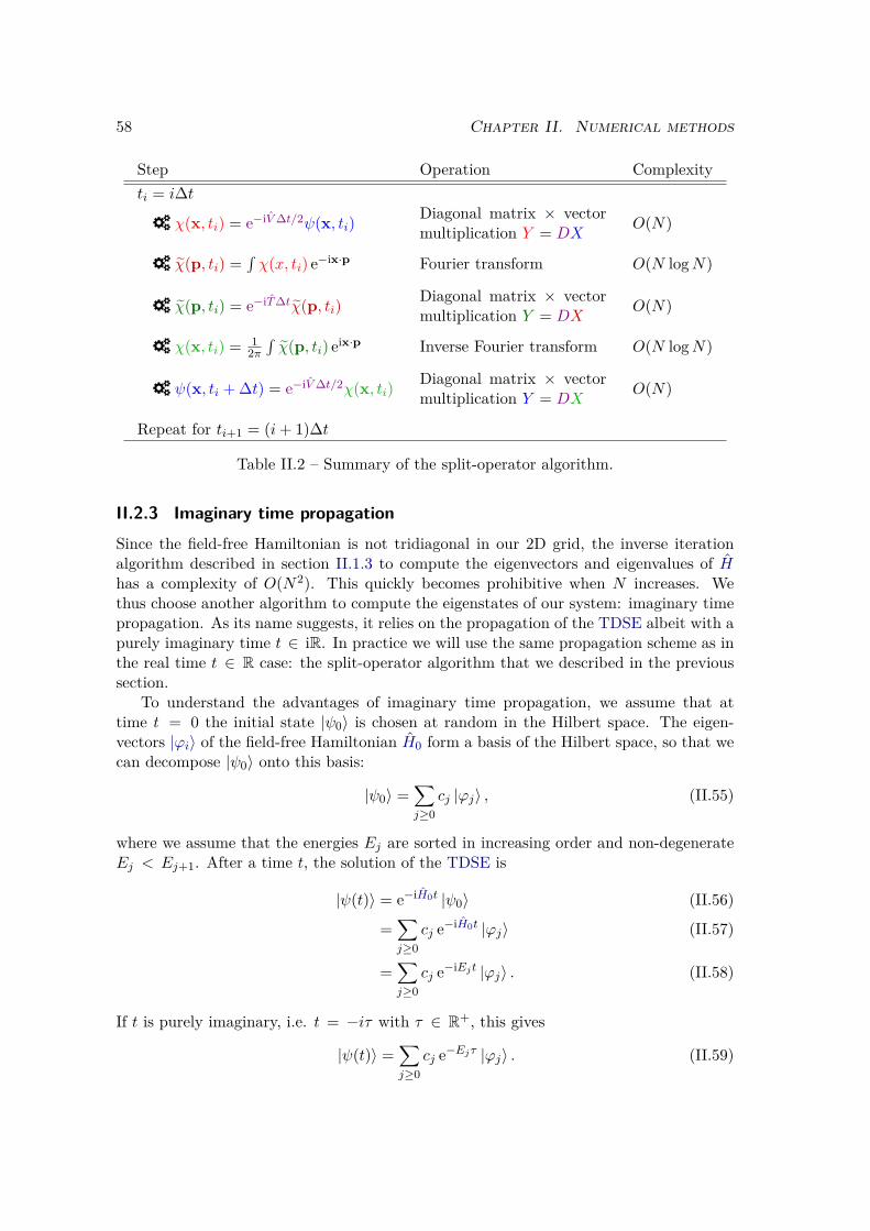
58 Chapter II. Numerical methods
Step Operation Complexityti = i∆t
3 χ(x, ti) = e−iV∆t/2ψ(x, ti)Diagonal matrix × vectormultiplication Y = DX
O(N)
3 χ(p, ti) =∫χ(x, ti) e−ix·p Fourier transform O(N logN)
3 χ(p, ti) = e−iT∆tχ(p, ti)Diagonal matrix × vectormultiplication Y = DX
O(N)
3 χ(x, ti) = 12π∫χ(p, ti) eix·p Inverse Fourier transform O(N logN)
3 ψ(x, ti + ∆t) = e−iV∆t/2χ(x, ti)Diagonal matrix × vectormultiplication Y = DX
O(N)
Repeat for ti+1 = (i+ 1)∆t
Table II.2 – Summary of the split-operator algorithm.
II.2.3 Imaginary time propagationSince the field-free Hamiltonian is not tridiagonal in our 2D grid, the inverse iterationalgorithm described in section II.1.3 to compute the eigenvectors and eigenvalues of Hhas a complexity of O(N2). This quickly becomes prohibitive when N increases. Wethus choose another algorithm to compute the eigenstates of our system: imaginary timepropagation. As its name suggests, it relies on the propagation of the TDSE albeit with apurely imaginary time t ∈ iR. In practice we will use the same propagation scheme as inthe real time t ∈ R case: the split-operator algorithm that we described in the previoussection.
To understand the advantages of imaginary time propagation, we assume that attime t = 0 the initial state |ψ0〉 is chosen at random in the Hilbert space. The eigen-vectors |ϕi〉 of the field-free Hamiltonian H0 form a basis of the Hilbert space, so that wecan decompose |ψ0〉 onto this basis:
|ψ0〉 =∑j≥0
cj |ϕj〉 , (II.55)
where we assume that the energies Ej are sorted in increasing order and non-degenerateEj < Ej+1. After a time t, the solution of the TDSE is
|ψ(t)〉 = e−iH0t |ψ0〉 (II.56)
=∑j≥0
cj e−iH0t |ϕj〉 (II.57)
=∑j≥0
cj e−iEjt |ϕj〉 . (II.58)
If t is purely imaginary, i.e. t = −iτ with τ ∈ R+, this gives
|ψ(t)〉 =∑j≥0
cj e−Ejτ |ϕj〉 . (II.59)
II.3 Wave function analysis 59
If c0 6= 0, we can factorize:
|ψ(t)〉 = c0 e−E0τ
|ϕ0〉+∑j≥1
cjc0
e−(Ej−E0)τ |ϕj〉
. (II.60)
Since E0 is the minimum of all Ej , Ej − E0 > 0 and all terms are exponentially dumpedwith respect to the first one. If we renormalize the wave function at each time step, orevery few time steps, it converges exponentially to the ground state of the system. Moregenerally, if all the i first coefficients are zero c0 = . . . = ci−1 = 0, and if we note ci thefirst non vanishing coefficient, we get
|ψ(t)〉 = ci e−Eiτ|ϕi〉+
∑j≥i+1
cjci
e−(Ej−Ei)τ |ϕj〉
. (II.61)
In this case, the renormalized wave function converges exponentially to state |ϕi〉.In practice we start by a random state with the appropriate symmetry and propagate
to get the ground state of the system. Once we have the ground state, we start againbut we orthonormalize at each time step, or every few time steps, the wave function withrespect to |ϕ0〉. We thus get the first excited state of the system. We then repeat this pro-cess, by orthonormalizing each time with respect to all previously computed eigenstates,until we get as many states as desired.
II.3 Wave function analysis
Once we know the time-dependent wave function |ψ(t)〉, in principle we know everythingabout the system’s dynamics. However the wave function in itself can be quite hardto interpret. If we take the example of HHG, the semi-classical model developed insection I.3.2 gave us more physical insight that the time-dependent wave function shownin Figure I.8. Moreover since the wave function is not directly measurable, we cannotuse it as such to analyze the results of an experiment. We thus resort to various analysistools to extract physical information from the wave function.
In general, these analysis tools rely on two basic quantities: the scalar product of twostates, which, in our case, is computed by
〈ϕ|ψ〉 =∑
xi∈gridϕ(xi)∗ψ(xi)
d∏j=1
∆xj , (II.62)
where d is the number of dimensions and ∆xj is the grid space step in dimension j. Andthe expectation value of an observable A, which is actually a particular case of (II.62):
〈A〉 = 〈ψ|A|ψ〉 =∑
xi∈gridψ(xi)∗A ψ(xi)
d∏j=1
∆xj . (II.63)
With these two basic operations we construct the tools we will use in this thesis.
60 Chapter II. Numerical methods
II.3.1 Ionization rate
a) Ionization probability
As we saw in section I.2.2, when an atom or a molecule is submitted to an electric field,it may be ionized. Consequently, the wave function can be separated into two orthogonalparts, a bound part and an ionized part:
|ψ(t)〉 = |ψbnd(t)〉+ |ψion(t)〉 , (II.64)
where the bound part can be decomposed onto the field-free bound states of the system:
|ψbnd(t)〉 =∑
i∈bound|ϕi〉 〈ϕi|ψ(t)〉 , (II.65)
and the ionized part can be similarly decomposed onto the field-free continuum states.The ionization probability at time t can be deduced from the norm of the ionized part,
which itself is deduced from the norm of the bound part:
Pion(t) = 〈ψion(t)|ψion(t)〉 (II.66)= 1− 〈ψbnd(t)|ψbnd(t)〉 (II.67)= 1−
∑i∈bound
|〈ϕi|ψ(t)〉|2. (II.68)
With equation (II.68) we can deduce the ionization probability from the populationsin all bound states. These populations are computed on the grid with the general for-mula (II.62). In this thesis we are generally far from any resonance, so that the popula-tions in the excited states |ϕi〉 quickly become negligible for growing values of i. We thusonly need to compute the populations in the first few bound states to get an accurateevaluation of the ionization probability.
b) Ionization rate in a static electric field
In the particular case of a static electric field, the population in the bound states expo-nentially decreases with time:
Pbnd(t) =∑
i∈bound|〈ϕi|ψ(t)〉|2 = e−Γt . (II.69)
The decay rate Γ is called the ionization rate. In the framework of non-Hermitian quantummechanics (see e.g. [146]) where the energies can be complex, this rate is directly relatedto the imaginary part of the energy ε0(FL) of the perturbed ground state:
ε0(FL) = E0(FL)− iΓ2 . (II.70)
Indeed, the perturbed ground state |ϕ0〉 evolves under the TDSE as:
|ψ(t)〉 = e−iHt |ϕ0〉 (II.71)
= e−iE0t e−Γt/2 |ϕ0〉 . (II.72)
II.3 Wave function analysis 61
Since the Hamiltonian is not Hermitian, the norm of this wave function is not conserved.Because only |ϕ0〉 is populated, the norm is equal to the population in the perturbedground state, and reads:
〈ψ(t)|ψ(t)〉 = |〈ϕ0|ψ(t)〉|2 = e−Γt, (II.73)
where we recognize the exponential decay of (II.69). Since |ϕ0〉 can be decomposed ontothe basis of the field-free bound states of H0, the population in this state is equal to thepopulation Pbnd in all bound states. Besides, using first order time-independent perturba-tion theory [135], we can show that the states that contribute most in this decompositionare those that are the closest to the ground state in energy. This justifies the restrictionto the first few bound states in the computation of Pbnd.
In practice, to compute the ionization rate Γ in a constant field F0, we start thepropagation in the field-free ground state |ϕ0〉. The electric field is initially zero, and isthen smoothly brought to its constant value by a sine square ramp:
FL(t) =
F0 sin2(Ωt) if 0 ≤ t ≤ π
2ΩF0 if π
2Ω ≤ t. (II.74)
Once the field is constant, we compute the population Pbnd in the first few (typically five)bound states, and we deduce the ionization rate Γ by
Γ = − 1Pbnd
dPbnddt . (II.75)
II.3.2 HHG spectrum
a) Dipole operators
The HHG spectrum consists of the power spectrum of the radiation emitted by the system.Three different forms of the dipole are commonly used to compute this power spectrum:the dipole (II.76a), velocity (II.76b) and acceleration forms (II.76c), which give the spectra
Sd(ω) =∣∣∣∣∫ 〈ψ(t)|Dd|ψ(t)〉 e−iωt
∣∣∣∣2 (II.76a)
Sv(ω) =∣∣∣∣∫ 〈ψ(t)|Dv|ψ(t)〉 e−iωt
∣∣∣∣2 (II.76b)
Sa(ω) =∣∣∣∣∫ 〈ψ(t)|Da|ψ(t)〉 e−iωt
∣∣∣∣2, (II.76c)
where Dd is the dipole operator, and where the velocity Dv and acceleration Da dipoleoperators are defined with the Ehrenfest theorem [151]:
Dd = r (II.77a)
D(l)v = i
[Hl, r
]= p (II.77b)
D(v)v = i
[Hv, r
]= p + AL(t) (II.77c)
Da = −[H,[H, r
]]+ dDv
dt = −∇V0 − FL(t). (II.77d)
62 Chapter II. Numerical methods
Note that the velocity dipole operator does not commute with r, and its definition is thusdifferent if we are in length (II.77b) or velocity (II.77c) gauge for the interaction with thelaser field (be careful not to be confused between the length and velocity gauge for theEM field, and the length, velocity and acceleration form of the dipole). We remind that,as discussed in section I.1.3, the operators may depend on the gauge but obviously theiraverage value, when computed exactly, does not.
The average value of the three dipole forms are related by
⟨Da⟩
=d⟨Dv⟩
dt (II.78)
⟨Dv⟩
=d⟨Dd⟩
dt . (II.79)
Therefore, if we integrate (II.76a) by part:∫〈ψ(t)|Dd|ψ(t)〉 e−iωt = 1
iω
∫〈ψ(t)|Dv|ψ(t)〉 e−iωt (II.80)
= − 1ω2
∫〈ψ(t)|Da|ψ(t)〉 e−iωt, (II.81)
we can relate the different power spectra:
ω2Sd = Sv = 1ω2Sa. (II.82)
We can therefore choose any dipole operator (II.77) to compute the spectrum, and thenmultiply by the appropriate factor of ω to get the desired form Sd, Sv or Sa. In practicewe will compute the average value of the acceleration dipole Da because, for numericalreasons, it is generally less noisy at high frequencies [152].
There are no clear consensus on which form of Sd, Sv or Sa should be used to get theHHG spectrum. An accelerated classical dipole emits a radiation whose total power, givenby the Larmor formula [78], is proportional to the square of the dipole acceleration. Onecould conclude that the acceleration form is more adapted. Nevertheless it was recentlyshown by Baggesen and Madsen [131] that the electric field of the emitted radiation alongthe laser propagation direction is proportional to the velocity dipole. We will thus usethe velocity form Sv. In practice we will compute Sa by taking the square modulus ofthe Fourier transform of the average value of the acceleration dipole (II.76c) and we willthen divide by ω2 (II.82) to get the velocity form of the power spectrum Sv.
b) Time-Frequency analysis
As we saw in sections I.3.2 and I.3.3, according to the 3-step model, each harmonicfrequency of the spectrum is actually emitted at a different time: the return time ofthe electron. The different harmonics thus have different phases and are not perfectlysynchronized. This results in a chirp of the emitted radiation, called atto-chirp [153–156]. However, we cannot get any information on this time of emission from the HHGpower spectrum. It is theoretically encoded in the phase of the Fourier transform of thedipole, but this is difficult to translate in emission times. To extract these harmonics
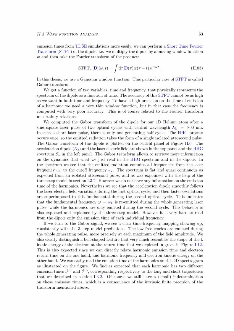
II.3 Wave function analysis 63
emission times from TDSE simulations more easily, we can perform a Short Time FourierTransform (STFT) of the dipole, i.e. we multiply the dipole by a moving window functionw and then take the Fourier transform of the product:
STFTw[D](ω, t) =∫
dτ D(τ)w(τ − t) e−iωτ . (II.83)
In this thesis, we use a Gaussian window function. This particular case of STFT is calledGabor transform.
We get a function of two variables, time and frequency, that physically represents thespectrum of the dipole as a function of time. The accuracy of this STFT cannot be as highas we want in both time and frequency. To have a high precision on the time of emissionof a harmonic we need a very thin window function, but in that case the frequency iscomputed with very poor accuracy. This is of course related to the Fourier transformuncertainty relations.
We computed the Gabor transform of the dipole for our 1D Helium atom after asine square laser pulse of two optical cycles with central wavelength λL = 800 nm.In such a short laser pulse, there is only one generating half cycle. The HHG processoccurs once, so the emitted radiation takes the form of a single isolated attosecond pulse.The Gabor transform of the dipole is plotted on the central panel of Figure II.6. Theacceleration dipole 〈Da〉 and the laser electric field are shown in the top panel and the HHGspectrum Sv in the left panel. The Gabor transform allows to retrieve more informationon the dynamics that what we just read in the HHG spectrum and in the dipole. Inthe spectrum we see that the emitted radiation contains all frequencies from the laserfrequency ωL to the cutoff frequency ωc. The spectrum is flat and quasi continuous asexpected from an isolated attosecond pulse, and as was explained with the help of thethree step model in section I.3.2. However we do not have any information on the emissiontime of the harmonics. Nevertheless we see that the acceleration dipole smoothly followsthe laser electric field variations during the first optical cycle, and then faster oscillationsare superimposed to this fundamental during the second optical cycle. This indicatesthat the fundamental frequency ω = ωL is re-emitted during the whole generating laserpulse, while the harmonics are only emitted during the second cycle. This behavior isalso expected and explained by the three step model. However it is very hard to readfrom the dipole only the emission time of each individual frequency.
If we turn to the Gabor signal, we see a clear time-frequency mapping showing up,consistently with the 3-step model predictions. The low frequencies are emitted duringthe whole generating pulse, more precisely at each maximum of the field amplitude. Wealso clearly distinguish a bell-shaped feature that very much resembles the shape of the kinetic energy of the electron at the return time that we depicted in green in Figure I.12.This is also expected since we can directly relate harmonic emission time and electronreturn time on the one hand, and harmonic frequency and electron kinetic energy on theother hand. We can easily read the emission time of the harmonics on this 2D spectrogramas illustrated on the figure. We find as expected that each harmonic has two differentemission times t(L) and t(S), corresponding respectively to the long and short trajectoriesthat we described in section I.3.2. Of course we still have a (small) indeterminationon these emission times, which is a consequence of the intrinsic finite precision of thetransform mentioned above.
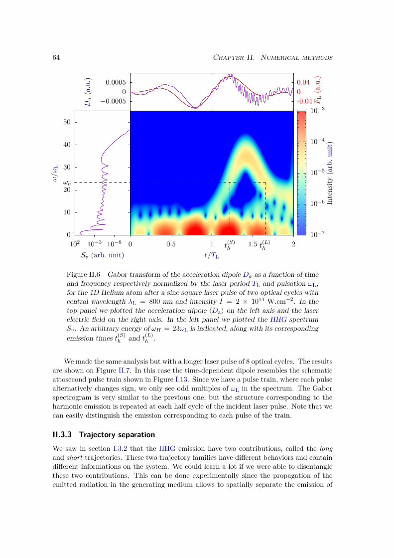
64 Chapter II. Numerical methods
0 0.5 1 1.5 2
ωh
t(S)h t
(L)h
0
10
20
30
40
50
10−810−3102
−0.00050
0.0005
-0.0400.04
t/TL
10−7
10−6
10−5
10−4
10−3
Intensity
(arb.
unit)
ω/ω
L
Sv (arb. unit)
Da(a.u.)
FL(a.u.)
Figure II.6 Gabor transform of the acceleration dipole Da as a function of timeand frequency respectively normalized by the laser period TL and pulsation ωL,for the 1D Helium atom after a sine square laser pulse of two optical cycles withcentral wavelength λL = 800 nm and intensity I = 2 × 10¹⁴ W.cm−2. In thetop panel we plotted the acceleration dipole 〈Da〉 on the left axis and the laserelectric field on the right axis. In the left panel we plotted the HHG spectrumSv. An arbitrary energy of ωH = 23ωL is indicated, along with its correspondingemission times t(S)
h and t(L)h .
We made the same analysis but with a longer laser pulse of 8 optical cycles. The resultsare shown on Figure II.7. In this case the time-dependent dipole resembles the schematicattosecond pulse train shown in Figure I.13. Since we have a pulse train, where each pulsealternatively changes sign, we only see odd multiples of ωL in the spectrum. The Gaborspectrogram is very similar to the previous one, but the structure corresponding to theharmonic emission is repeated at each half cycle of the incident laser pulse. Note that wecan easily distinguish the emission corresponding to each pulse of the train.
II.3.3 Trajectory separationWe saw in section I.3.2 that the HHG emission have two contributions, called the longand short trajectories. These two trajectory families have different behaviors and containdifferent informations on the system. We could learn a lot if we were able to disentanglethese two contributions. This can be done experimentally since the propagation of theemitted radiation in the generating medium allows to spatially separate the emission of
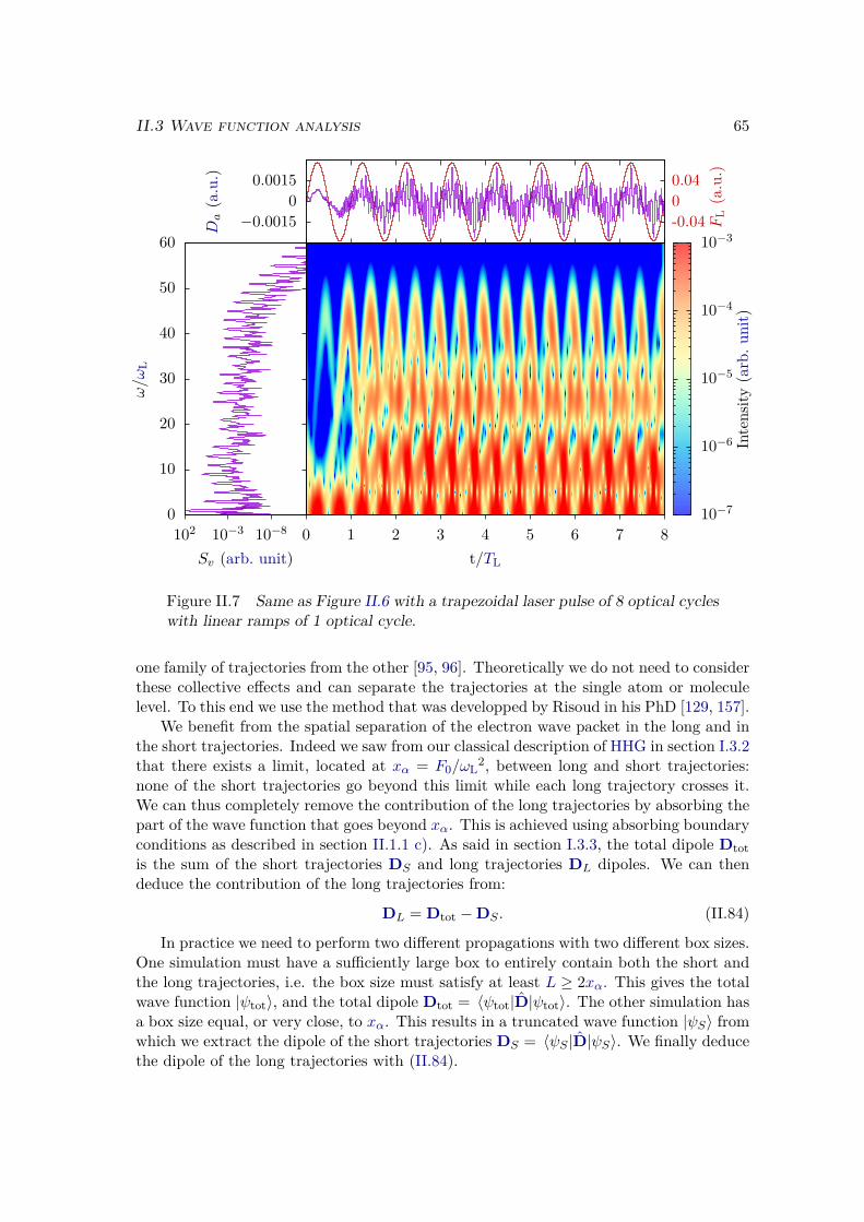
II.3 Wave function analysis 65
0 1 2 3 4 5 6 7 80
10
20
30
40
50
60
10−810−3102
−0.00150
0.0015
-0.0400.04
t/TL
10−7
10−6
10−5
10−4
10−3
Intensity
(arb.
unit)
ω/ω
L
Sv (arb. unit)
Da(a.u.)
FL(a.u.)
Figure II.7 Same as Figure II.6 with a trapezoidal laser pulse of 8 optical cycleswith linear ramps of 1 optical cycle.
one family of trajectories from the other [95, 96]. Theoretically we do not need to considerthese collective effects and can separate the trajectories at the single atom or moleculelevel. To this end we use the method that was developped by Risoud in his PhD [129, 157].
We benefit from the spatial separation of the electron wave packet in the long and inthe short trajectories. Indeed we saw from our classical description of HHG in section I.3.2that there exists a limit, located at xα = F0/ωL
2, between long and short trajectories:none of the short trajectories go beyond this limit while each long trajectory crosses it.We can thus completely remove the contribution of the long trajectories by absorbing thepart of the wave function that goes beyond xα. This is achieved using absorbing boundaryconditions as described in section II.1.1 c). As said in section I.3.3, the total dipole Dtotis the sum of the short trajectories DS and long trajectories DL dipoles. We can thendeduce the contribution of the long trajectories from:
DL = Dtot −DS . (II.84)
In practice we need to perform two different propagations with two different box sizes.One simulation must have a sufficiently large box to entirely contain both the short andthe long trajectories, i.e. the box size must satisfy at least L ≥ 2xα. This gives the totalwave function |ψtot〉, and the total dipole Dtot = 〈ψtot|D|ψtot〉. The other simulation hasa box size equal, or very close, to xα. This results in a truncated wave function |ψS〉 fromwhich we extract the dipole of the short trajectories DS = 〈ψS |D|ψS〉. We finally deducethe dipole of the long trajectories with (II.84).
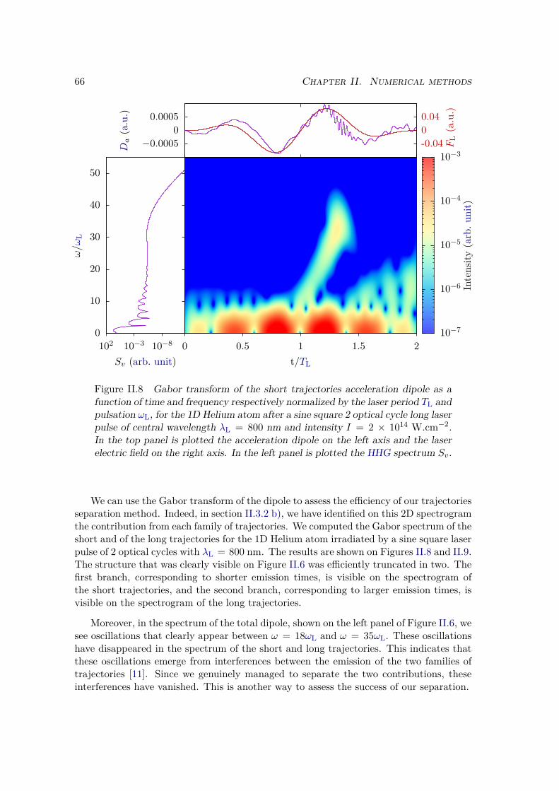
66 Chapter II. Numerical methods
0 0.5 1 1.5 20
10
20
30
40
50
10−810−3102
−0.00050
0.0005
-0.0400.04
t/TL
10−7
10−6
10−5
10−4
10−3
Intensity
(arb.
unit)
ω/ω
L
Sv (arb. unit)
Da(a.u.)
FL(a.u.)
Figure II.8 Gabor transform of the short trajectories acceleration dipole as afunction of time and frequency respectively normalized by the laser period TL andpulsation ωL, for the 1D Helium atom after a sine square 2 optical cycle long laserpulse of central wavelength λL = 800 nm and intensity I = 2 × 10¹⁴ W.cm−2.In the top panel is plotted the acceleration dipole on the left axis and the laserelectric field on the right axis. In the left panel is plotted the HHG spectrum Sv.
We can use the Gabor transform of the dipole to assess the efficiency of our trajectoriesseparation method. Indeed, in section II.3.2 b), we have identified on this 2D spectrogramthe contribution from each family of trajectories. We computed the Gabor spectrum of theshort and of the long trajectories for the 1D Helium atom irradiated by a sine square laserpulse of 2 optical cycles with λL = 800 nm. The results are shown on Figures II.8 and II.9.The structure that was clearly visible on Figure II.6 was efficiently truncated in two. Thefirst branch, corresponding to shorter emission times, is visible on the spectrogram ofthe short trajectories, and the second branch, corresponding to larger emission times, isvisible on the spectrogram of the long trajectories.
Moreover, in the spectrum of the total dipole, shown on the left panel of Figure II.6, wesee oscillations that clearly appear between ω = 18ωL and ω = 35ωL. These oscillationshave disappeared in the spectrum of the short and long trajectories. This indicates thatthese oscillations emerge from interferences between the emission of the two families oftrajectories [11]. Since we genuinely managed to separate the two contributions, theseinterferences have vanished. This is another way to assess the success of our separation.
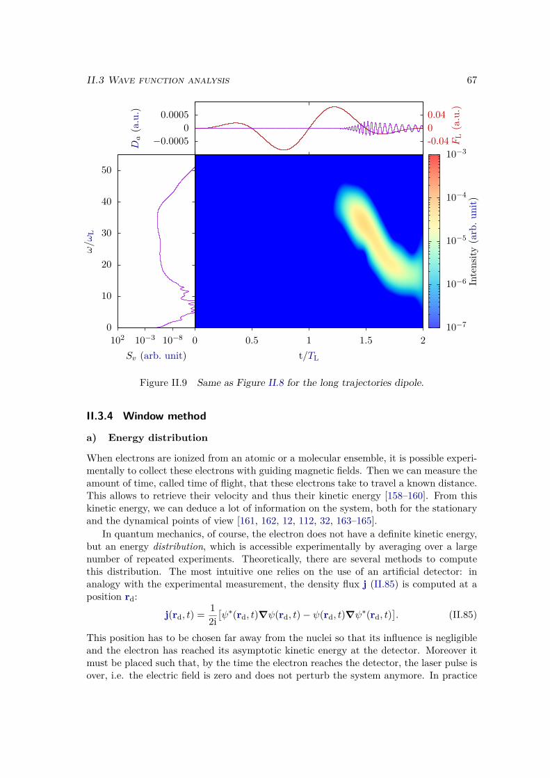
II.3 Wave function analysis 67
0 0.5 1 1.5 20
10
20
30
40
50
10−810−3102
−0.00050
0.0005
-0.0400.04
t/TL
10−7
10−6
10−5
10−4
10−3
Intensity
(arb.
unit)
ω/ω
L
Sv (arb. unit)
Da(a.u.)
FL(a.u.)
Figure II.9 Same as Figure II.8 for the long trajectories dipole.
II.3.4 Window method
a) Energy distribution
When electrons are ionized from an atomic or a molecular ensemble, it is possible experi-mentally to collect these electrons with guiding magnetic fields. Then we can measure theamount of time, called time of flight, that these electrons take to travel a known distance.This allows to retrieve their velocity and thus their kinetic energy [158–160]. From thiskinetic energy, we can deduce a lot of information on the system, both for the stationaryand the dynamical points of view [161, 162, 12, 112, 32, 163–165].
In quantum mechanics, of course, the electron does not have a definite kinetic energy,but an energy distribution, which is accessible experimentally by averaging over a largenumber of repeated experiments. Theoretically, there are several methods to computethis distribution. The most intuitive one relies on the use of an artificial detector: inanalogy with the experimental measurement, the density flux j (II.85) is computed at aposition rd:
j(rd, t) = 12i[ψ∗(rd, t)∇ψ(rd, t)− ψ(rd, t)∇ψ∗(rd, t)
]. (II.85)
This position has to be chosen far away from the nuclei so that its influence is negligibleand the electron has reached its asymptotic kinetic energy at the detector. Moreover itmust be placed such that, by the time the electron reaches the detector, the laser pulse isover, i.e. the electric field is zero and does not perturb the system anymore. In practice
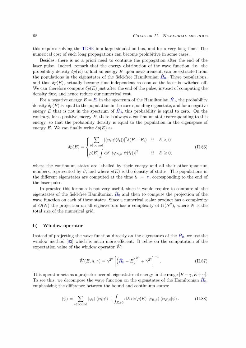
68 Chapter II. Numerical methods
this requires solving the TDSE in a large simulation box, and for a very long time. Thenumerical cost of such long propagations can become prohibitive in some cases.
Besides, there is no a priori need to continue the propagation after the end of thelaser pulse. Indeed, remark that the energy distribution of the wave function, i.e. theprobability density δp(E) to find an energy E upon measurement, can be extracted fromthe populations in the eigenstates of the field-free Hamiltonian H0. These populations,and thus δp(E), actually become time-independent as soon as the laser is switched off.We can therefore compute δp(E) just after the end of the pulse, instead of computing thedensity flux, and hence reduce our numerical cost.
For a negative energy E = Ei in the spectrum of the Hamiltonian H0, the probabilitydensity δp(E) is equal to the population in the corresponding eigenstate, and for a negativeenergy E that is not in the spectrum of H0, this probability is equal to zero. On thecontrary, for a positive energy E, there is always a continuum state corresponding to thisenergy, so that the probability density is equal to the population in the eigenspace ofenergy E. We can finally write δp(E) as
δp(E) =
∑
i∈bound|〈ϕi|ψ(tf)〉|2δ(E − Ei) if E < 0
ρ(E)∫
dβ |〈ϕE,β|ψ(tf)〉|2 if E ≥ 0,(II.86)
where the continuum states are labelled by their energy and all their other quantumnumbers, represented by β, and where ρ(E) is the density of states. The populations inthe different eigenstates are computed at the time tf = τL corresponding to the end ofthe laser pulse.
In practice this formula is not very useful, since it would require to compute all theeigenstates of the field-free Hamiltonian H0 and then to compute the projection of thewave function on each of these states. Since a numerical scalar product has a complexityof O(N) the projection on all eigenvectors has a complexity of O(N2), where N is thetotal size of the numerical grid.
b) Window operator
Instead of projecting the wave function directly on the eigenstates of the H0, we use thewindow method [82] which is much more efficient. It relies on the computation of theexpectation value of the window operator W :
W (E,n, γ) = γ2n[(H0 − E
)2n+ γ2n
]−1. (II.87)
This operator acts as a projector over all eigenstates of energy in the range [E − γ,E + γ].To see this, we decompose the wave function on the eigenstates of the Hamiltonian H0,emphasizing the difference between the bound and continuum states:
|ψ〉 =∑
i∈bound|ϕi〉 〈ϕi|ψ〉+
∫E>0
dE dβ ρ(E) |ϕE,β〉 〈ϕE,β|ψ〉 . (II.88)
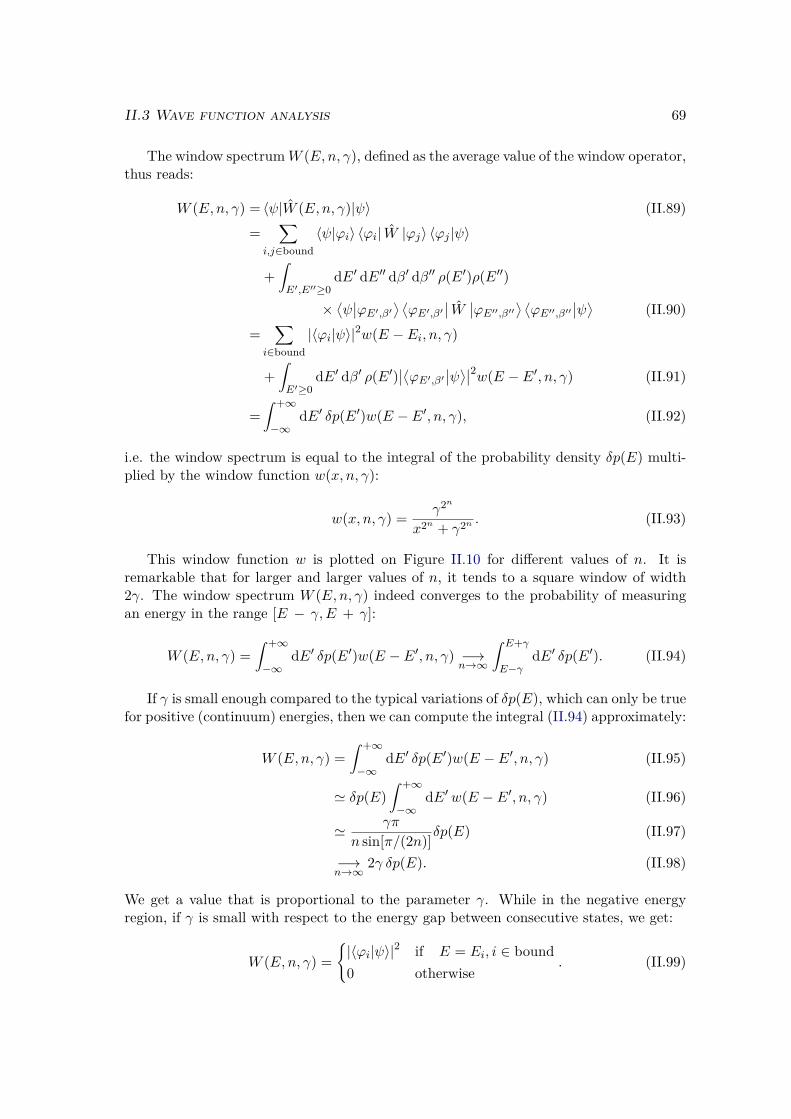
II.3 Wave function analysis 69
The window spectrumW (E,n, γ), defined as the average value of the window operator,thus reads:
W (E,n, γ) = 〈ψ|W (E,n, γ)|ψ〉 (II.89)=
∑i,j∈bound
〈ψ|ϕi〉 〈ϕi| W |ϕj〉 〈ϕj |ψ〉
+∫E′,E′′≥0
dE′ dE′′ dβ′ dβ′′ ρ(E′)ρ(E′′)
×⟨ψ∣∣ϕE′,β′⟩ ⟨ϕE′,β′∣∣ W ∣∣ϕE′′,β′′⟩ ⟨ϕE′′,β′′ ∣∣ψ⟩ (II.90)
=∑
i∈bound|〈ϕi|ψ〉|2w(E − Ei, n, γ)
+∫E′≥0
dE′ dβ′ ρ(E′)∣∣⟨ϕE′,β′ ∣∣ψ⟩∣∣2w(E − E′, n, γ) (II.91)
=∫ +∞
−∞dE′ δp(E′)w(E − E′, n, γ), (II.92)
i.e. the window spectrum is equal to the integral of the probability density δp(E) multi-plied by the window function w(x, n, γ):
w(x, n, γ) = γ2n
x2n + γ2n . (II.93)
This window function w is plotted on Figure II.10 for different values of n. It isremarkable that for larger and larger values of n, it tends to a square window of width2γ. The window spectrum W (E,n, γ) indeed converges to the probability of measuringan energy in the range [E − γ,E + γ]:
W (E,n, γ) =∫ +∞
−∞dE′ δp(E′)w(E − E′, n, γ) −→
n→∞
∫ E+γ
E−γdE′ δp(E′). (II.94)
If γ is small enough compared to the typical variations of δp(E), which can only be truefor positive (continuum) energies, then we can compute the integral (II.94) approximately:
W (E,n, γ) =∫ +∞
−∞dE′ δp(E′)w(E − E′, n, γ) (II.95)
' δp(E)∫ +∞
−∞dE′w(E − E′, n, γ) (II.96)
' γπ
n sin[π/(2n)]δp(E) (II.97)
−→n→∞
2γ δp(E). (II.98)
We get a value that is proportional to the parameter γ. While in the negative energyregion, if γ is small with respect to the energy gap between consecutive states, we get:
W (E,n, γ) =|〈ϕi|ψ〉|2 if E = Ei, i ∈ bound0 otherwise
. (II.99)
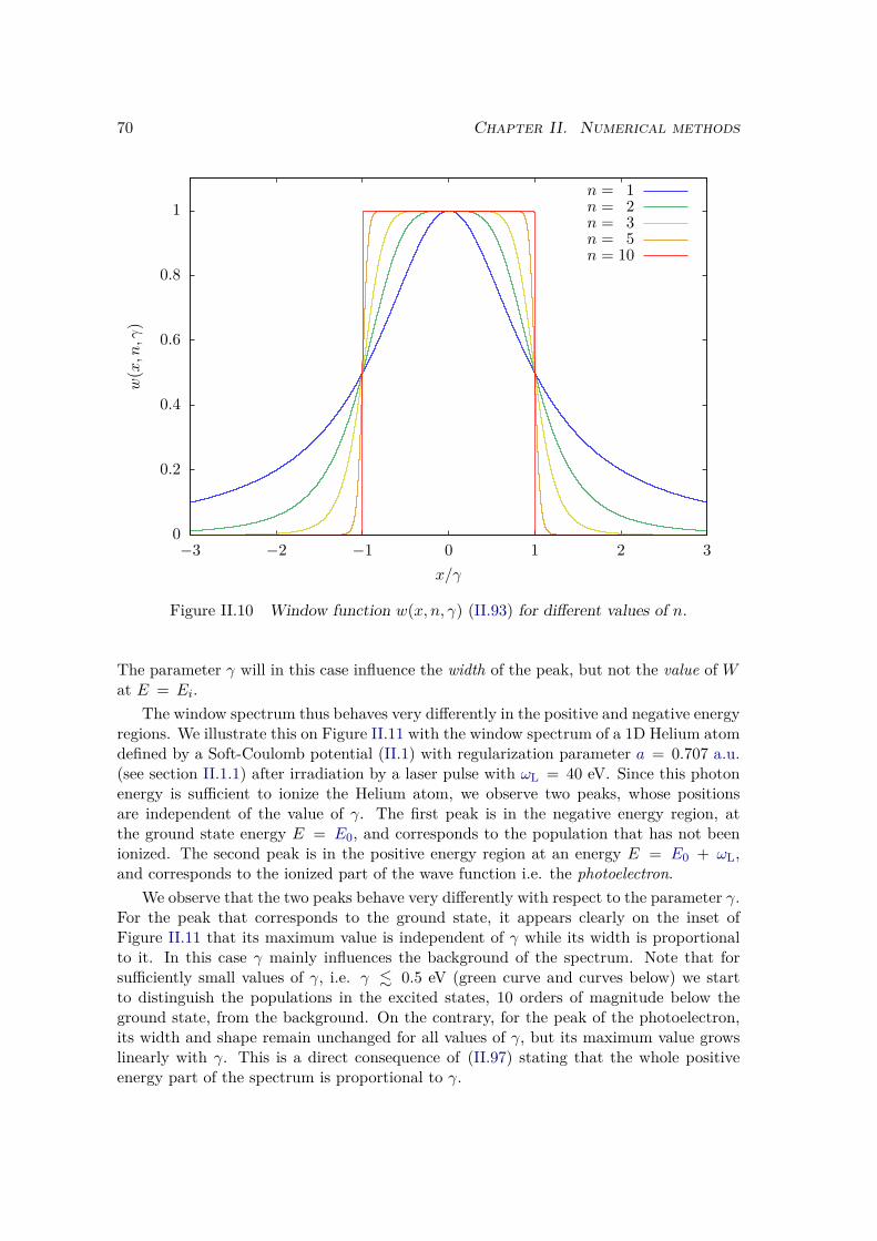
70 Chapter II. Numerical methods
0
0.2
0.4
0.6
0.8
1
−3 −2 −1 0 1 2 3
w(x,n,γ
)
x/γ
n = 1n = 2n = 3n = 5n = 10
Figure II.10 Window function w(x, n, γ) (II.93) for different values of n.
The parameter γ will in this case influence the width of the peak, but not the value of Wat E = Ei.
The window spectrum thus behaves very differently in the positive and negative energyregions. We illustrate this on Figure II.11 with the window spectrum of a 1D Helium atomdefined by a Soft-Coulomb potential (II.1) with regularization parameter a = 0.707 a.u.(see section II.1.1) after irradiation by a laser pulse with ωL = 40 eV. Since this photonenergy is sufficient to ionize the Helium atom, we observe two peaks, whose positionsare independent of the value of γ. The first peak is in the negative energy region, atthe ground state energy E = E0, and corresponds to the population that has not beenionized. The second peak is in the positive energy region at an energy E = E0 + ωL,and corresponds to the ionized part of the wave function i.e. the photoelectron.
We observe that the two peaks behave very differently with respect to the parameter γ.For the peak that corresponds to the ground state, it appears clearly on the inset ofFigure II.11 that its maximum value is independent of γ while its width is proportionalto it. In this case γ mainly influences the background of the spectrum. Note that forsufficiently small values of γ, i.e. γ . 0.5 eV (green curve and curves below) we startto distinguish the populations in the excited states, 10 orders of magnitude below theground state, from the background. On the contrary, for the peak of the photoelectron,its width and shape remain unchanged for all values of γ, but its maximum value growslinearly with γ. This is a direct consequence of (II.97) stating that the whole positiveenergy part of the spectrum is proportional to γ.
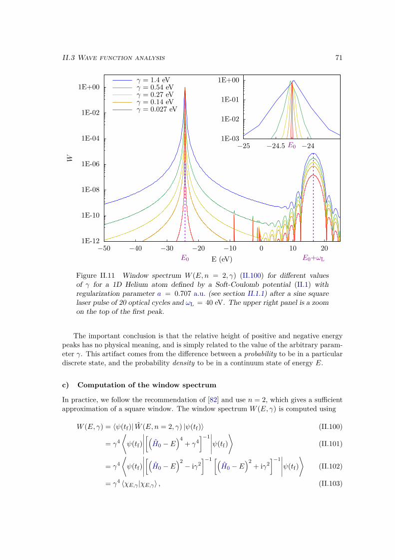
II.3 Wave function analysis 71
1E-12
1E-10
1E-08
1E-06
1E-04
1E-02
1E+00
−50 −40 −30 −20 −10 0 10 20E0 E0+ωL
1E-03
1E-02
1E-01
1E+00
−25 −24.5 −24E0 E0+ωL
W
E (eV)
γ = 1.4 eVγ = 0.54 eVγ = 0.27 eVγ = 0.14 eVγ = 0.027 eV
Figure II.11 Window spectrum W (E,n = 2, γ) (II.100) for different valuesof γ for a 1D Helium atom defined by a Soft-Coulomb potential (II.1) withregularization parameter a = 0.707 a.u. (see section II.1.1) after a sine squarelaser pulse of 20 optical cycles and ωL = 40 eV. The upper right panel is a zoomon the top of the first peak.
The important conclusion is that the relative height of positive and negative energypeaks has no physical meaning, and is simply related to the value of the arbitrary param-eter γ. This artifact comes from the difference between a probability to be in a particulardiscrete state, and the probability density to be in a continuum state of energy E.
c) Computation of the window spectrum
In practice, we follow the recommendation of [82] and use n = 2, which gives a sufficientapproximation of a square window. The window spectrum W (E, γ) is computed using
W (E, γ) = 〈ψ(tf)| W (E,n = 2, γ) |ψ(tf)〉 (II.100)
= γ4⟨ψ(tf)
∣∣∣∣∣[(H0 − E
)4+ γ4
]−1∣∣∣∣∣ψ(tf)
⟩(II.101)
= γ4⟨ψ(tf)
∣∣∣∣∣[(H0 − E
)2− iγ2
]−1 [(H0 − E
)2+ iγ2
]−1∣∣∣∣∣ψ(tf)
⟩(II.102)
= γ4 〈χE,γ |χE,γ〉 , (II.103)
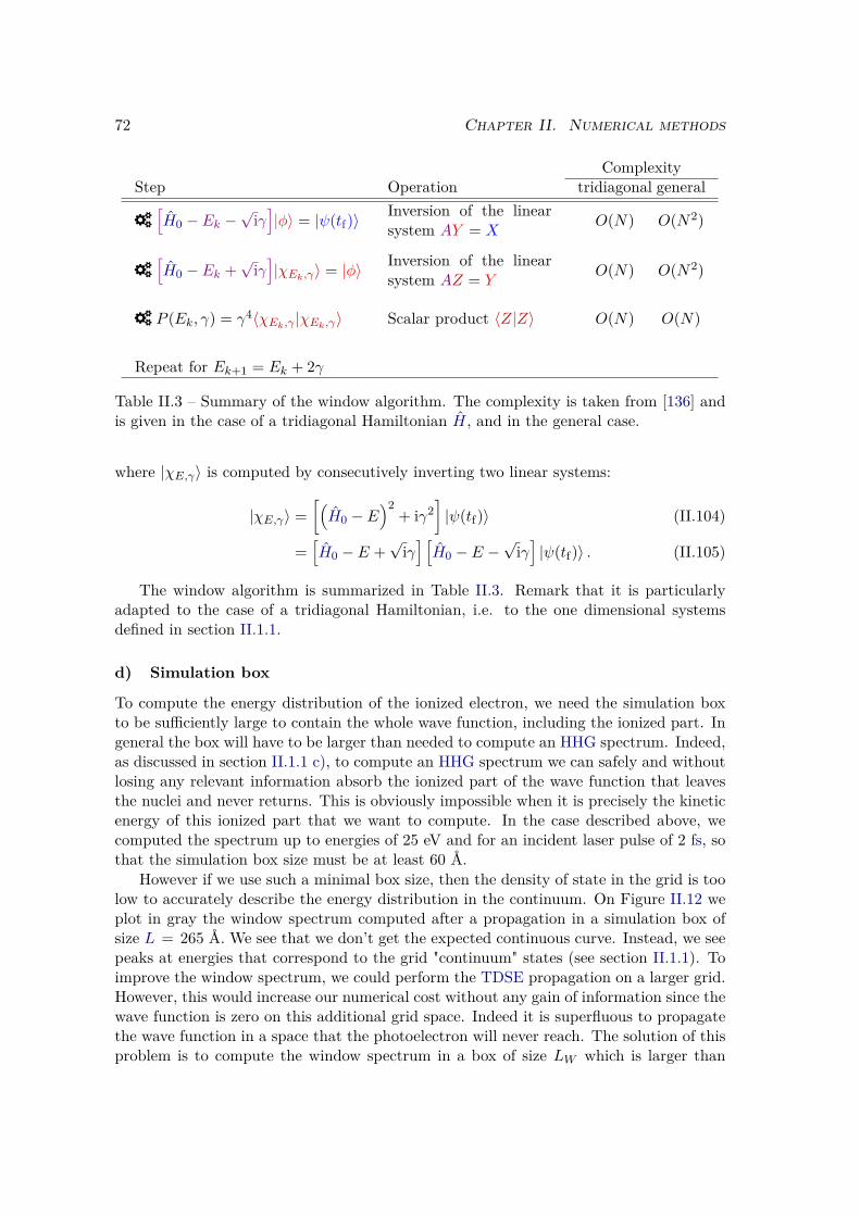
72 Chapter II. Numerical methods
ComplexityStep Operation tridiagonal general
3[H0 − Ek −
√iγ]|φ〉 = |ψ(tf)〉
Inversion of the linearsystem AY = X
O(N) O(N2)
3[H0 − Ek +
√iγ]|χEk,γ〉 = |φ〉 Inversion of the linear
system AZ = YO(N) O(N2)
3 P (Ek, γ) = γ4〈χEk,γ |χEk,γ〉 Scalar product 〈Z|Z〉 O(N) O(N)
Repeat for Ek+1 = Ek + 2γ
Table II.3 – Summary of the window algorithm. The complexity is taken from [136] andis given in the case of a tridiagonal Hamiltonian H, and in the general case.
where |χE,γ〉 is computed by consecutively inverting two linear systems:
|χE,γ〉 =[(H0 − E
)2+ iγ2
]|ψ(tf)〉 (II.104)
=[H0 − E +
√iγ] [H0 − E −
√iγ]|ψ(tf)〉 . (II.105)
The window algorithm is summarized in Table II.3. Remark that it is particularlyadapted to the case of a tridiagonal Hamiltonian, i.e. to the one dimensional systemsdefined in section II.1.1.
d) Simulation box
To compute the energy distribution of the ionized electron, we need the simulation boxto be sufficiently large to contain the whole wave function, including the ionized part. Ingeneral the box will have to be larger than needed to compute an HHG spectrum. Indeed,as discussed in section II.1.1 c), to compute an HHG spectrum we can safely and withoutlosing any relevant information absorb the ionized part of the wave function that leavesthe nuclei and never returns. This is obviously impossible when it is precisely the kineticenergy of this ionized part that we want to compute. In the case described above, wecomputed the spectrum up to energies of 25 eV and for an incident laser pulse of 2 fs, sothat the simulation box size must be at least 60 Å.
However if we use such a minimal box size, then the density of state in the grid is toolow to accurately describe the energy distribution in the continuum. On Figure II.12 weplot in gray the window spectrum computed after a propagation in a simulation box ofsize L = 265 Å. We see that we don’t get the expected continuous curve. Instead, we seepeaks at energies that correspond to the grid "continuum" states (see section II.1.1). Toimprove the window spectrum, we could perform the TDSE propagation on a larger grid.However, this would increase our numerical cost without any gain of information since thewave function is zero on this additional grid space. Indeed it is superfluous to propagatethe wave function in a space that the photoelectron will never reach. The solution of thisproblem is to compute the window spectrum in a box of size LW which is larger than
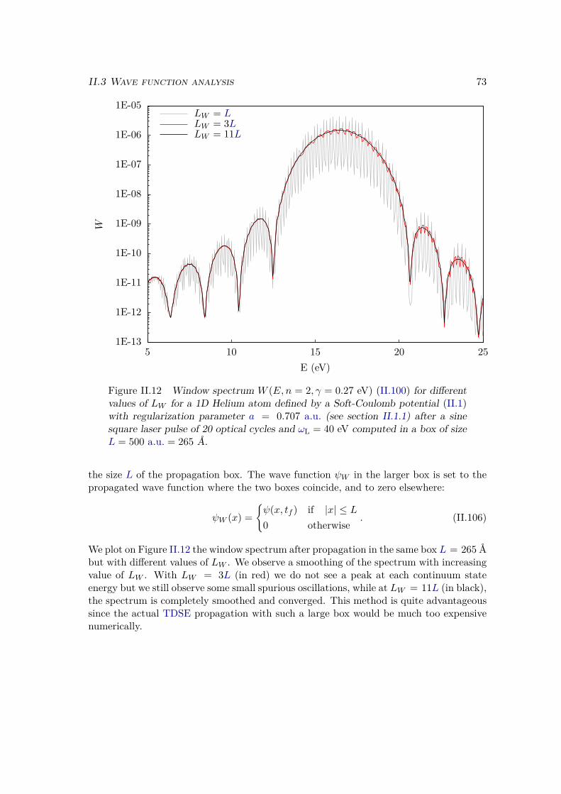
II.3 Wave function analysis 73
1E-13
1E-12
1E-11
1E-10
1E-09
1E-08
1E-07
1E-06
1E-05
5 10 15 20 25
W
E (eV)
LW = LLW = 3LLW = 11L
Figure II.12 Window spectrum W (E,n = 2, γ = 0.27 eV) (II.100) for differentvalues of LW for a 1D Helium atom defined by a Soft-Coulomb potential (II.1)with regularization parameter a = 0.707 a.u. (see section II.1.1) after a sinesquare laser pulse of 20 optical cycles and ωL = 40 eV computed in a box of sizeL = 500 a.u. = 265 Å.
the size L of the propagation box. The wave function ψW in the larger box is set to thepropagated wave function where the two boxes coincide, and to zero elsewhere:
ψW (x) =ψ(x, tf ) if |x| ≤ L0 otherwise
. (II.106)
We plot on Figure II.12 the window spectrum after propagation in the same box L = 265 Åbut with different values of LW . We observe a smoothing of the spectrum with increasingvalue of LW . With LW = 3L (in red) we do not see a peak at each continuum stateenergy but we still observe some small spurious oscillations, while at LW = 11L (in black),the spectrum is completely smoothed and converged. This method is quite advantageoussince the actual TDSE propagation with such a large box would be much too expensivenumerically.

74 Chapter II. Numerical methods
Chapter IIITunnel ionization
As reviewed in Chapter I, the interaction between an atom or a molecule and an electricfield can give rise to various phenomena depending on the considered time and energyscales. At low frequencies (typically infrared radiation) and high intensities (1013 W.cm−2
and beyond), we saw that the ionization of the system by a laser can no longer be describedby the absorption of one or several photons depicted by perturbation theory. In suchconditions, the laser field strongly distorts the atomic potential so that electrons canescape through tunnel effect. This phenomenon was first modeled by Keldysh [113] inthe 60’s and was then intensively investigated, since it represents the first step of thehighly non-linear processes that we described in section I.3, such as HHG [91, 96], ornon-sequential multiple ionization [94].
As for many non-linear processes, the only way to accurately describe tunnel ionizationis to numerically solve the TDSE. However, because of its high numerical cost, this methodcan only be used for small systems, i.e. an atom with one or two electrons. The descriptionof larger and more complex systems such as molecules is very delicate and requires someapproximations: Single Active Electron approximation and frozen nuclei [166–168], StrongField Approximation [169, 170] or low dimensionality [171]. On the other hand, onemay rely on approximate models such as the Lewenstein model [11] that we reviewed insection I.3.3, or the Quantitative ReScattering theory [59]. The advantage of these modelsis to yield analytical formulas and derivations that are easier to handle than numericalsimulations. Moreover, they allow to decompose each strong field process into differentsteps, e.g. the celebrated three-step model for HHG [9, 91], which provides valuablephysical pictures and insights. As we have seen, tunnel ionization is the universal firststep of all recollision processes, and is also the main source of their non-linearity, henceits central importance in strong field physics.
For all the reasons we just cited, approximate analytical formulas, see [172, 173] formore complete reviews, are often prefered to numerical simulations for the analysis andinterpretation of experimental results. The most frequently used formulas rely on theadiabatic approximation, which holds when the Keldysh parameter, defined in (I.69), isvery small γ 1. Among them are the ones derived by Perelomov, Popov and Terent’ev(PPT) [174–176] or Ammosov, Delone and Krainov (ADK) [177] for atoms, and extendedto molecules (Mo-ADK) by Tong et al. [178, 179] and Kjeldsen and Madsen [180], but alsomore advanced analytical works like the ones performed by Tolstikhin et al. [181, 182].However, these analytical formulas have a limited accuracy as was extensively shown
75
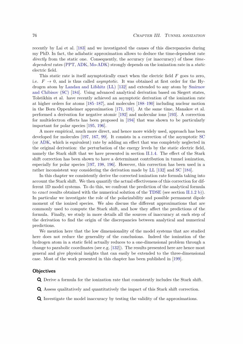
76 Chapter III. Tunnel ionization
recently by Lai et al. [183] and we investigated the causes of this discrepancies duringmy PhD. In fact, the adiabatic approximation allows to deduce the time-dependent ratedirectly from the static one. Consequently, the accuracy (or inaccuracy) of these time-dependent rates (PPT, ADK, Mo-ADK) strongly depends on the ionization rate in a staticelectric field.
This static rate is itself asymptotically exact when the electric field F goes to zero,i.e. F → 0, and is thus called asymptotic. It was obtained at first order for the Hy-drogen atom by Landau and Lifshitz (LL) [132] and extended to any atom by Smirnovand Chibisov (SC) [184]. Using advanced analytical derivation based on Siegert states,Tolstikhin et al. have recently achieved an asymptotic derivation of the ionization rateat higher orders for atoms [185–187], and molecules [188–190] including nuclear motionin the Born Oppenheimer approximation [171, 191]. At the same time, Manakov et al.performed a derivation for negative atomic [192] and molecular ions [193]. A correctionfor multielectron effects has been proposed in [194] that was shown to be particularlyimportant for polar species [195, 196].
A more empirical, much more direct, and hence more widely used, approach has beendeveloped for molecules [197, 167, 99]. It consists in a correction of the asymptotic SC(or ADK, which is equivalent) rate by adding an effect that was completely neglected inthe original derivation: the perturbation of the energy levels by the static electric field,namely the Stark shift that we have presented in section II.1.4. The effect of the Starkshift correction has been shown to have a determinant contribution in tunnel ionization,especially for polar species [197, 198, 196]. However, this correction has been used in arather inconsistent way considering the derivation made by LL [132] and SC [184].
In this chapter we consistently derive the corrected ionization rate formula taking intoaccount the Stark shift. We then quantify the actual effectiveness of this correction for dif-ferent 1D model systems. To do this, we confront the prediction of the analytical formulato exact results obtained with the numerical solution of the TDSE (see section II.1.2 b)).In particular we investigate the role of the polarizability and possible permanent dipolemoment of the ionized species. We also discuss the different approximations that arecommonly used to compute the Stark shift, and how they affect the predictions of theformula. Finally, we study in more details all the sources of inaccuracy at each step ofthe derivation to find the origin of the discrepancies between analytical and numericalpredictions.
We mention here that the low dimensionality of the model systems that are studiedhere does not reduce the generality of the conclusions. Indeed the ionization of thehydrogen atom in a static field actually reduces to a one-dimensional problem through achange to parabolic coordinates (see e.g. [132]). The results presented here are hence mostgeneral and give physical insights that can easily be extended to the three-dimensionalcase. Most of the work presented in this chapter has been published in [199].
Objectives
ü Derive a formula for the ionization rate that consistently includes the Stark shift.
ü Assess qualitatively and quantitatively the impact of this Stark shift correction.
ü Investigate the model inaccuracy by testing the validity of the approximations.
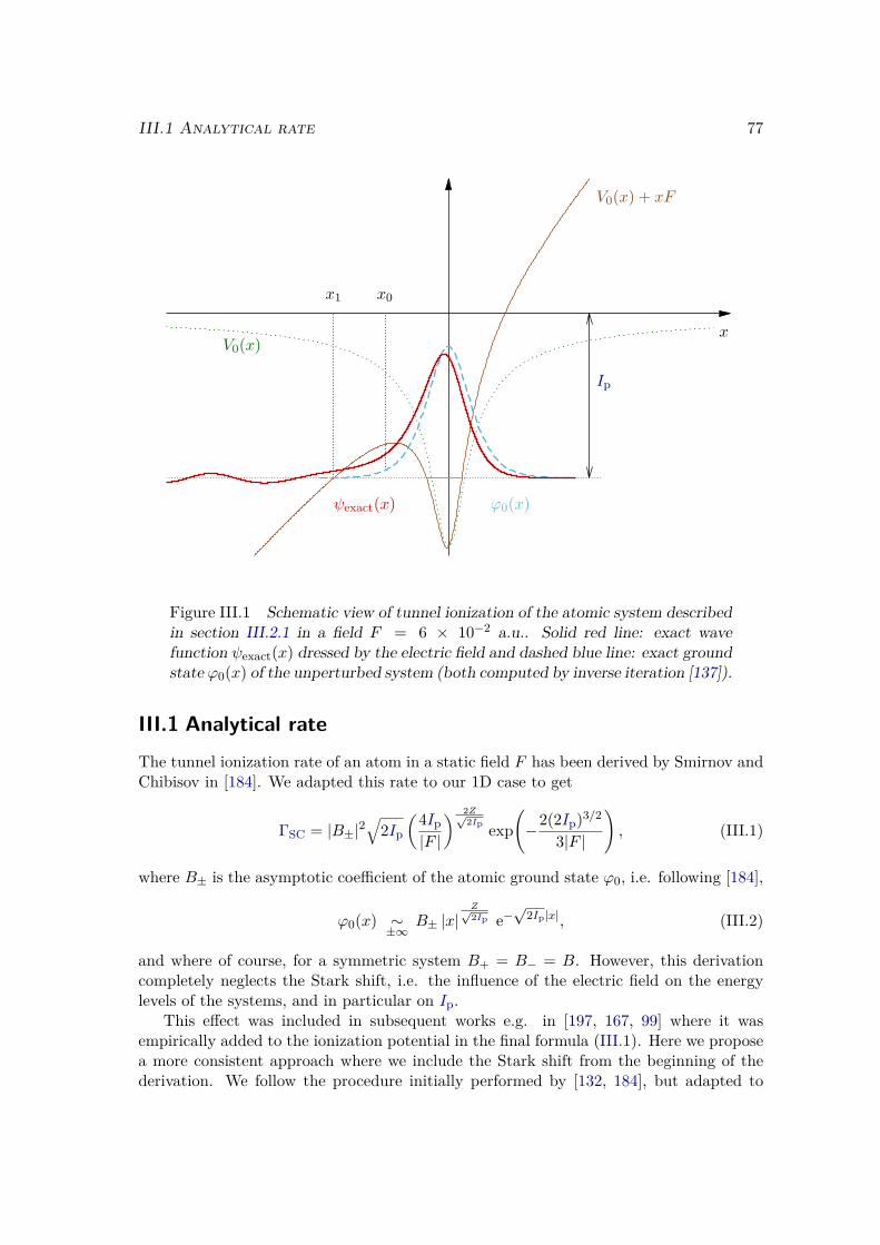
III.1 Analytical rate 77
x0x1
Ip
ϕ0(x)ψexact(x)
V0(x) + xF
V0(x)x
Figure III.1 Schematic view of tunnel ionization of the atomic system describedin section III.2.1 in a field F = 6 × 10⁻² a.u.. Solid red line: exact wavefunction ψexact(x) dressed by the electric field and dashed blue line: exact groundstate ϕ0(x) of the unperturbed system (both computed by inverse iteration [137]).
III.1 Analytical rateThe tunnel ionization rate of an atom in a static field F has been derived by Smirnov andChibisov in [184]. We adapted this rate to our 1D case to get
ΓSC = |B±|2√
2Ip
(4Ip|F |
) 2Z√2Ip exp
(−2(2Ip)3/2
3|F |
), (III.1)
where B± is the asymptotic coefficient of the atomic ground state ϕ0, i.e. following [184],
ϕ0(x) ∼±∞
B± |x|Z√2Ip e−
√2Ip|x|, (III.2)
and where of course, for a symmetric system B+ = B− = B. However, this derivationcompletely neglects the Stark shift, i.e. the influence of the electric field on the energylevels of the systems, and in particular on Ip.
This effect was included in subsequent works e.g. in [197, 167, 99] where it wasempirically added to the ionization potential in the final formula (III.1). Here we proposea more consistent approach where we include the Stark shift from the beginning of thederivation. We follow the procedure initially performed by [132, 184], but adapted to
78 Chapter III. Tunnel ionization
our one dimensional case. To recover the three dimensional rate, one should integratethe formula over the two remaining variables, as it is done in [132, 184]. Note that allthe approximations that are made in this section will be extensively discussed later, insection III.3.
We consider the system depicted in Figure III.1 composed of an electron trapped ina potential well V0 like e.g. the Soft Coulomb potential described in section II.1.1. Wedo not need to actually specify the shape of V0 near the nuclei. We only suppose thatit behaves asymptotically like a Coulomb potential. We place this bound electron in avery weak static electric field F (2Ip)3/2. We denote by Ip = Ip + ∆Ip the correctedionization potential that include the Stark shift ∆Ip. For a weak electric field, the Starkshift can be treated through perturbation theory, and ∆Ip Ip. For a symmetricpotential, the choice of sign of the electric field is irrelevant and we choose F positive,therefore ionization occurs in the region of space where x is negative. Note that theelectric field induces a strong asymmetry, and that the ionization occurs only in the xnegative region of space.
The ionization rate Γ can be computed as the electronic density flux far from theatomic potential, i.e. at a point x → −∞, out of the wave function ψ(x) correspondingto the ground state dressed by the electric field:
Γ = − Im(ψ∗dψdx ). (III.3)
However, the wave function is not available in most practical cases, we thus use thesemi-classical approximate expression:
ψ(x) =
C√p
exp(
i∫ x1
xp(x′) dx′ − iπ
4
), x < x1
C ′√|p|
exp(∫ x
x1
∣∣p(x′)∣∣ dx′) , x1 < x ≤ x0 ,
(III.4)
where p(x) =√
2(−Ip − V0(x)− xF ) is the classical action, x1 is the external turningpoint i.e. p(x1) = 0, and where x0 is a point inside the potential energy barrier, as depictedon Figure III.1. This point x0 is chosen sufficiently close to zero so that the influence ofthe field is negligible |x0F | Ip, and also sufficiently far so that the influence of thepotential is also negligible |V0(x0)| Ip. Note that the electric field needs to be verysmall for these two assumptions not to be contradictory. We will come back to this later.Using the connecting formulas in [132], we find the relations between C and C ′, and wecan express the wave function as
ψ(x) =
C√p
exp(
i∫ x1
xp(x′) dx′ − iπ
4
), x < x1
C√|p|
exp(∫ x
x1
∣∣p(x′)∣∣ dx′ + iπ2
), x1 < x ≤ x0 .
(III.5)
We got the wave function up to a constant factor C. The computation of this factor relieson a choice of normalization, of which the absolute value of the rate will depend, since ifwe insert (III.5) in (III.3) the rate becomes:
Γ = |C|2. (III.6)
III.1 Analytical rate 79
The choice of Landau and Lifshitz in [132] and Smirnov and Chibisov in [184] is toconnect the semi-classical wave function with the ground state ϕ0 of the unperturbedsystem. To this end, in the same way as LL, we use |x0F | Ip, to neglect the influenceof the electric field on the wave function close to zero:
ψ(x) = ϕ0(x), x0 ≤ x ≤ 0. (III.7)
Using the continuity of the wave function at x0, this allows to determines the constant Cand the final expression for ψ(x) outside the barrier:
ψ(x) = ϕ0(x0)√|p(x0)|√p(x)
exp(−∫ x0
x1
∣∣p(x′)∣∣ dx′) exp(
i∫ x1
xp(x′) dx′ − 3iπ
4
), x < x1,
(III.8)
and thus the ionization rate:
Γ = |ϕ0(x0)|2 |p(x0)| exp(−2∫ x0
x1
∣∣p(x′)∣∣ dx′) . (III.9)
Remark that this expression does not depend on the point x at which the electronicdensity flux is evaluated, which is satisfactory.
We need to compute the three factors of this product. First, in the preexponentialfactor we use both |x0F | Ip and |V0(x0)| Ip to approximate |p(x0)| '
√2Ip.
Second, in the exponential we keep the first two terms of the expansion of |p(x)| inpowers of V0(x)/(xF + Ip):
|p(x)| =√
2(xF + Ip) + V0(x)√2(xF + Ip)
+O
(V0(x)2
(xF + Ip) 32
)(III.10)
which, after integration gives
∫ x0
x1|p(x)|dx = (2Ip) 3
2
3F (1 + η)32 − Z√
2Ip
ln(
1 +√
1 + η
1−√
1 + η
)+O
(Z
32F
12
Ip32
), (III.11)
whereη = |x0F |/Ip. (III.12)
To be exhaustive, we have kept the factors in front of the powers of F in the O(Fα).We use η 1 to make the expansion
∫ x0
x1|p(x)| dx = (2Ip) 3
2
3F + x0
√2Ip
︸ ︷︷ ︸A
− Z√2Ip
ln(4η
+O(1))
︸ ︷︷ ︸B
+O
(x2
0F√Ip
)+O
(Z
32F
12
Ip32
). (III.13)
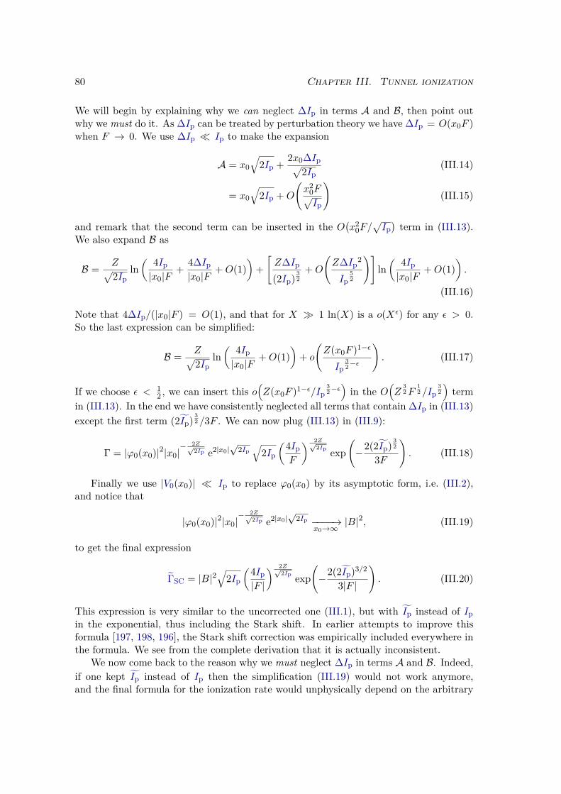
80 Chapter III. Tunnel ionization
We will begin by explaining why we can neglect ∆Ip in terms A and B, then point outwhy we must do it. As ∆Ip can be treated by perturbation theory we have ∆Ip = O(x0F )when F → 0. We use ∆Ip Ip to make the expansion
A = x0√
2Ip + 2x0∆Ip√2Ip
(III.14)
= x0√
2Ip +O
(x2
0F√Ip
)(III.15)
and remark that the second term can be inserted in the O(x2
0F/√Ip)term in (III.13).
We also expand B as
B = Z√2Ip
ln( 4Ip|x0|F
+ 4∆Ip|x0|F
+O(1))
+[Z∆Ip
(2Ip) 32
+O
(Z∆Ip
2
Ip52
)]ln( 4Ip|x0|F
+O(1)).
(III.16)
Note that 4∆Ip/(|x0|F ) = O(1), and that for X 1 ln(X) is a o(Xε) for any ε > 0.So the last expression can be simplified:
B = Z√2Ip
ln( 4Ip|x0|F
+O(1))
+ o
(Z(x0F )1−ε
Ip32−ε
). (III.17)
If we choose ε < 12 , we can insert this o
(Z(x0F )1−ε/Ip
32−ε)in the O
(Z
32F
12 /Ip
32)term
in (III.13). In the end we have consistently neglected all terms that contain ∆Ip in (III.13)except the first term (2Ip) 3
2 /3F . We can now plug (III.13) in (III.9):
Γ = |ϕ0(x0)|2|x0|− 2Z√
2Ip e2|x0|√
2Ip√
2Ip
(4IpF
) 2Z√2Ip exp
(−2(2Ip) 3
2
3F
). (III.18)
Finally we use |V0(x0)| Ip to replace ϕ0(x0) by its asymptotic form, i.e. (III.2),and notice that
|ϕ0(x0)|2|x0|− 2Z√
2Ip e2|x0|√
2Ip −−−−→x0→∞
|B|2, (III.19)
to get the final expression
ΓSC = |B|2√
2Ip
(4Ip|F |
) 2Z√2Ip exp
(−2(2Ip)3/2
3|F |
). (III.20)
This expression is very similar to the uncorrected one (III.1), but with Ip instead of Ipin the exponential, thus including the Stark shift. In earlier attempts to improve thisformula [197, 198, 196], the Stark shift correction was empirically included everywhere inthe formula. We see from the complete derivation that it is actually inconsistent.
We now come back to the reason why we must neglect ∆Ip in terms A and B. Indeed,if one kept Ip instead of Ip then the simplification (III.19) would not work anymore,and the final formula for the ionization rate would unphysically depend on the arbitrary
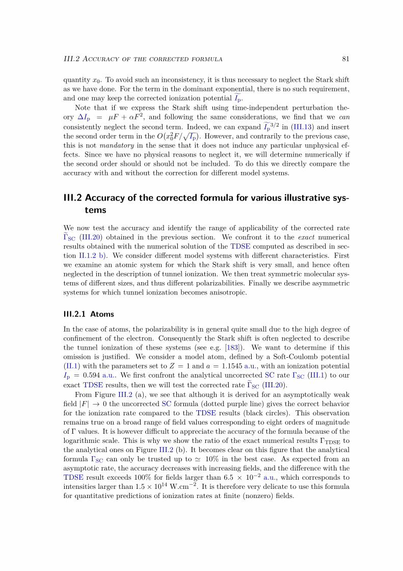
III.2 Accuracy of the corrected formula 81
quantity x0. To avoid such an inconsistency, it is thus necessary to neglect the Stark shiftas we have done. For the term in the dominant exponential, there is no such requirement,and one may keep the corrected ionization potential Ip.
Note that if we express the Stark shift using time-independent perturbation the-ory ∆Ip = µF + αF 2, and following the same considerations, we find that we canconsistently neglect the second term. Indeed, we can expand Ip
3/2 in (III.13) and insertthe second order term in the O
(x2
0F/√Ip). However, and contrarily to the previous case,
this is not mandatory in the sense that it does not induce any particular unphysical ef-fects. Since we have no physical reasons to neglect it, we will determine numerically ifthe second order should or should not be included. To do this we directly compare theaccuracy with and without the correction for different model systems.
III.2 Accuracy of the corrected formula for various illustrative sys-tems
We now test the accuracy and identify the range of applicability of the corrected rateΓSC (III.20) obtained in the previous section. We confront it to the exact numericalresults obtained with the numerical solution of the TDSE computed as described in sec-tion II.1.2 b). We consider different model systems with different characteristics. Firstwe examine an atomic system for which the Stark shift is very small, and hence oftenneglected in the description of tunnel ionization. We then treat symmetric molecular sys-tems of different sizes, and thus different polarizabilities. Finally we describe asymmetricsystems for which tunnel ionization becomes anisotropic.
III.2.1 Atoms
In the case of atoms, the polarizability is in general quite small due to the high degree ofconfinement of the electron. Consequently the Stark shift is often neglected to describethe tunnel ionization of these systems (see e.g. [183]). We want to determine if thisomission is justified. We consider a model atom, defined by a Soft-Coulomb potential(II.1) with the parameters set to Z = 1 and a = 1.1545 a.u., with an ionization potentialIp = 0.594 a.u.. We first confront the analytical uncorrected SC rate ΓSC (III.1) to ourexact TDSE results, then we will test the corrected rate ΓSC (III.20).
From Figure III.2 (a), we see that although it is derived for an asymptotically weakfield |F | → 0 the uncorrected SC formula (dotted purple line) gives the correct behaviorfor the ionization rate compared to the TDSE results (black circles). This observationremains true on a broad range of field values corresponding to eight orders of magnitudeof Γ values. It is however difficult to appreciate the accuracy of the formula because of thelogarithmic scale. This is why we show the ratio of the exact numerical results ΓTDSE tothe analytical ones on Figure III.2 (b). It becomes clear on this figure that the analyticalformula ΓSC can only be trusted up to ' 10% in the best case. As expected from anasymptotic rate, the accuracy decreases with increasing fields, and the difference with theTDSE result exceeds 100% for fields larger than 6.5 × 10⁻² a.u., which corresponds tointensities larger than 1.5 × 10¹⁴ W.cm−2. It is therefore very delicate to use this formulafor quantitative predictions of ionization rates at finite (nonzero) fields.
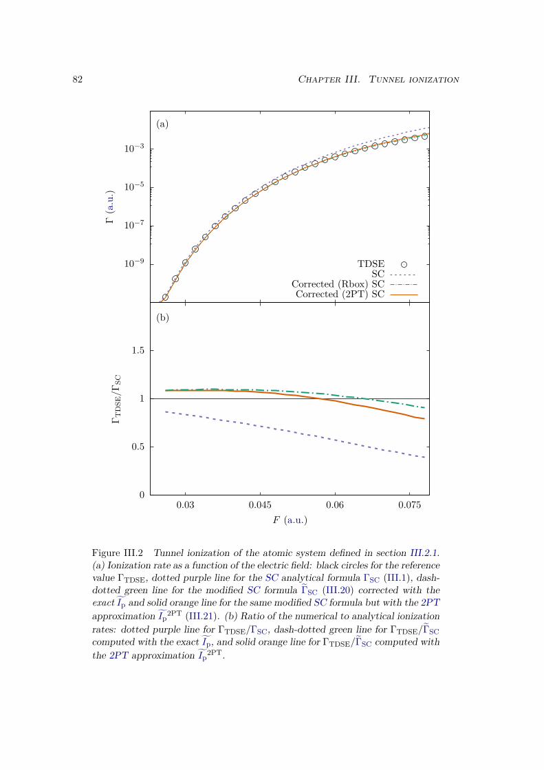
82 Chapter III. Tunnel ionization
10−9
10−7
10−5
10−3
(a)
0
0.5
1
1.5
0.03 0.045 0.06 0.075
(b)
Γ(a.u.)
TDSESC
Corrected (Rbox) SCCorrected (2PT) SC
Γ TD
SE/Γ S
C
F (a.u.)
Figure III.2 Tunnel ionization of the atomic system defined in section III.2.1.(a) Ionization rate as a function of the electric field: black circles for the referencevalue ΓTDSE, dotted purple line for the SC analytical formula ΓSC (III.1), dash-dotted green line for the modified SC formula ΓSC (III.20) corrected with theexact Ip and solid orange line for the same modified SC formula but with the 2PTapproximation Ip
2PT (III.21). (b) Ratio of the numerical to analytical ionizationrates: dotted purple line for ΓTDSE/ΓSC, dash-dotted green line for ΓTDSE/ΓSCcomputed with the exact Ip, and solid orange line for ΓTDSE/ΓSC computed withthe 2PT approximation Ip
2PT.
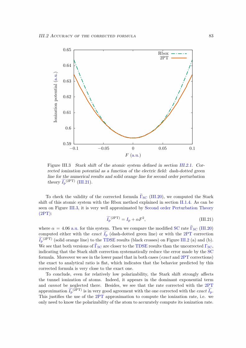
III.2 Accuracy of the corrected formula 83
0.59
0.6
0.61
0.62
0.63
0.64
0.65
−0.1 −0.05 0 0.05 0.1
Ionizatio
npo
tential(
a.u.)
F (a.u.)
Rbox2PT
Figure III.3 Stark shift of the atomic system defined in section III.2.1. Cor-rected ionization potential as a function of the electric field: dash-dotted greenline for the numerical results and solid orange line for second order perturbationtheory Ip
(2PT) (III.21).
To check the validity of the corrected formula ΓSC (III.20), we computed the Starkshift of this atomic system with the Rbox method explained in section II.1.4. As can beseen on Figure III.3, it is very well approximated by Second order Perturbation Theory(2PT):
Ip(2PT) = Ip + αF 2, (III.21)
where α = 4.06 a.u. for this system. Then we compare the modified SC rate ΓSC (III.20)computed either with the exact Ip (dash-dotted green line) or with the 2PT correctionIp
(2PT) (solid orange line) to the TDSE results (black crosses) on Figure III.2 (a) and (b).We see that both versions of ΓSC are closer to the TDSE results than the uncorrected ΓSC,indicating that the Stark shift correction systematically reduce the error made by the SCformula. Moreover we see in the lower panel that in both cases (exact and 2PT corrections)the exact to analytical ratio is flat, which indicates that the behavior predicted by thiscorrected formula is very close to the exact one.
To conclude, even for relatively low polarizability, the Stark shift strongly affectsthe tunnel ionization of atoms. Indeed, it appears in the dominant exponential termand cannot be neglected there. Besides, we see that the rate corrected with the 2PTapproximation Ip
(2PT) is in very good agreement with the one corrected with the exact Ip.This justifies the use of the 2PT approximation to compute the ionization rate, i.e. weonly need to know the polarizability of the atom to accurately compute its ionization rate.
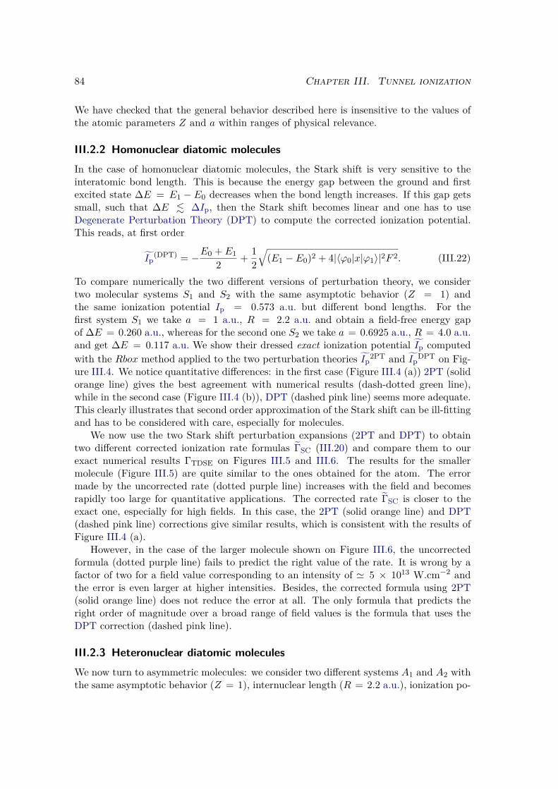
84 Chapter III. Tunnel ionization
We have checked that the general behavior described here is insensitive to the values ofthe atomic parameters Z and a within ranges of physical relevance.
III.2.2 Homonuclear diatomic moleculesIn the case of homonuclear diatomic molecules, the Stark shift is very sensitive to theinteratomic bond length. This is because the energy gap between the ground and firstexcited state ∆E = E1 − E0 decreases when the bond length increases. If this gap getssmall, such that ∆E . ∆Ip, then the Stark shift becomes linear and one has to useDegenerate Perturbation Theory (DPT) to compute the corrected ionization potential.This reads, at first order
Ip(DPT) = −E0 + E1
2 + 12
√(E1 − E0)2 + 4|〈ϕ0|x|ϕ1〉|2F 2. (III.22)
To compare numerically the two different versions of perturbation theory, we considertwo molecular systems S1 and S2 with the same asymptotic behavior (Z = 1) andthe same ionization potential Ip = 0.573 a.u. but different bond lengths. For thefirst system S1 we take a = 1 a.u., R = 2.2 a.u. and obtain a field-free energy gapof ∆E = 0.260 a.u., whereas for the second one S2 we take a = 0.6925 a.u., R = 4.0 a.u.and get ∆E = 0.117 a.u. We show their dressed exact ionization potential Ip computedwith the Rbox method applied to the two perturbation theories Ip
2PT and IpDPT on Fig-
ure III.4. We notice quantitative differences: in the first case (Figure III.4 (a)) 2PT (solidorange line) gives the best agreement with numerical results (dash-dotted green line),while in the second case (Figure III.4 (b)), DPT (dashed pink line) seems more adequate.This clearly illustrates that second order approximation of the Stark shift can be ill-fittingand has to be considered with care, especially for molecules.
We now use the two Stark shift perturbation expansions (2PT and DPT) to obtaintwo different corrected ionization rate formulas ΓSC (III.20) and compare them to ourexact numerical results ΓTDSE on Figures III.5 and III.6. The results for the smallermolecule (Figure III.5) are quite similar to the ones obtained for the atom. The errormade by the uncorrected rate (dotted purple line) increases with the field and becomesrapidly too large for quantitative applications. The corrected rate ΓSC is closer to theexact one, especially for high fields. In this case, the 2PT (solid orange line) and DPT(dashed pink line) corrections give similar results, which is consistent with the results ofFigure III.4 (a).
However, in the case of the larger molecule shown on Figure III.6, the uncorrectedformula (dotted purple line) fails to predict the right value of the rate. It is wrong by afactor of two for a field value corresponding to an intensity of ' 5 × 10¹³ W.cm−2 andthe error is even larger at higher intensities. Besides, the corrected formula using 2PT(solid orange line) does not reduce the error at all. The only formula that predicts theright order of magnitude over a broad range of field values is the formula that uses theDPT correction (dashed pink line).
III.2.3 Heteronuclear diatomic moleculesWe now turn to asymmetric molecules: we consider two different systems A1 and A2 withthe same asymptotic behavior (Z = 1), internuclear length (R = 2.2 a.u.), ionization po-
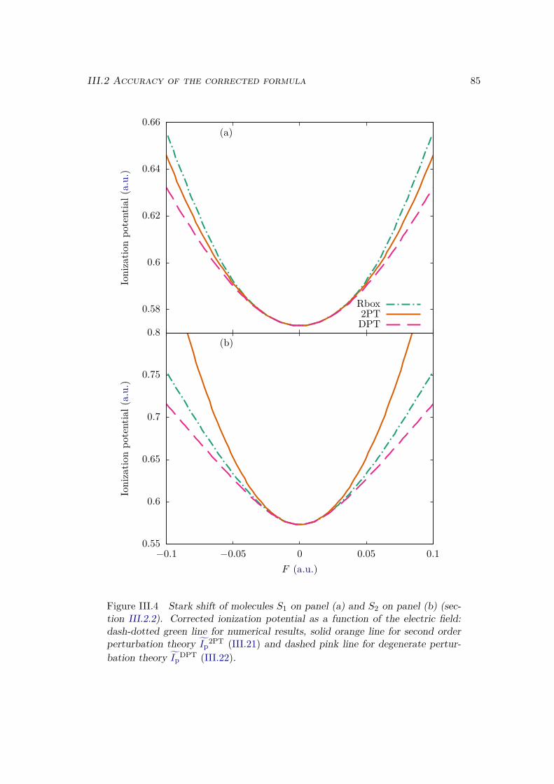
III.2 Accuracy of the corrected formula 85
0.58
0.6
0.62
0.64
0.66(a)
0.55
0.6
0.65
0.7
0.75
0.8
−0.1 −0.05 0 0.05 0.1
(b)
Ionizatio
npo
tential(
a.u.)
Rbox2PTDPT
Ionizatio
npo
tential(
a.u.)
F (a.u.)
Figure III.4 Stark shift of molecules S1 on panel (a) and S2 on panel (b) (sec-tion III.2.2). Corrected ionization potential as a function of the electric field:dash-dotted green line for numerical results, solid orange line for second orderperturbation theory Ip
2PT (III.21) and dashed pink line for degenerate pertur-bation theory Ip
DPT (III.22).
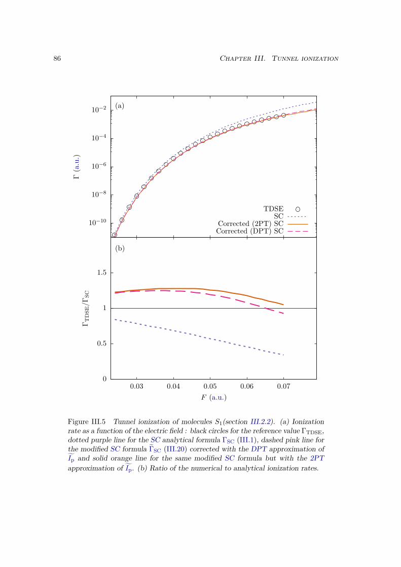
86 Chapter III. Tunnel ionization
10−10
10−8
10−6
10−4
10−2 (a)
0
0.5
1
1.5
0.03 0.04 0.05 0.06 0.07
(b)
Γ(a.u.)
TDSESC
Corrected (2PT) SCCorrected (DPT) SC
Γ TD
SE/Γ S
C
F (a.u.)
Figure III.5 Tunnel ionization of molecules S1(section III.2.2). (a) Ionizationrate as a function of the electric field : black circles for the reference value ΓTDSE,dotted purple line for the SC analytical formula ΓSC (III.1), dashed pink line forthe modified SC formula ΓSC (III.20) corrected with the DPT approximation ofIp and solid orange line for the same modified SC formula but with the 2PTapproximation of Ip. (b) Ratio of the numerical to analytical ionization rates.
III.2 Accuracy of the corrected formula 87
10−10
10−8
10−6
10−4
10−2 (a)
1
0
2
4
6
8
0.03 0.04 0.05 0.06 0.07
(b)
Γ(a.u.)
TDSESC
Corrected (2PT) SCCorrected (DPT) SC
Γ TD
SE/Γ S
C
F (a.u.)
Figure III.6 Same as in Figure III.5 for the molecule S2.
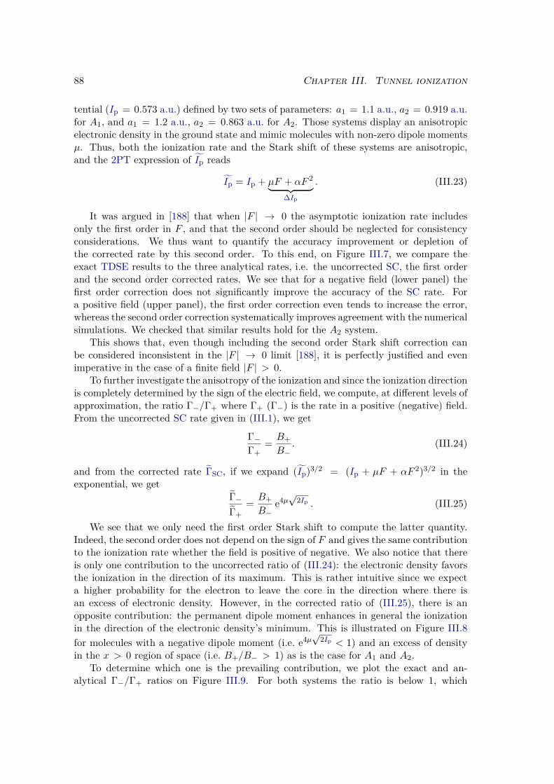
88 Chapter III. Tunnel ionization
tential (Ip = 0.573 a.u.) defined by two sets of parameters: a1 = 1.1 a.u., a2 = 0.919 a.u.for A1, and a1 = 1.2 a.u., a2 = 0.863 a.u. for A2. Those systems display an anisotropicelectronic density in the ground state and mimic molecules with non-zero dipole momentsµ. Thus, both the ionization rate and the Stark shift of these systems are anisotropic,and the 2PT expression of Ip reads
Ip = Ip + µF + αF 2︸ ︷︷ ︸∆Ip
. (III.23)
It was argued in [188] that when |F | → 0 the asymptotic ionization rate includesonly the first order in F , and that the second order should be neglected for consistencyconsiderations. We thus want to quantify the accuracy improvement or depletion ofthe corrected rate by this second order. To this end, on Figure III.7, we compare theexact TDSE results to the three analytical rates, i.e. the uncorrected SC, the first orderand the second order corrected rates. We see that for a negative field (lower panel) thefirst order correction does not significantly improve the accuracy of the SC rate. Fora positive field (upper panel), the first order correction even tends to increase the error,whereas the second order correction systematically improves agreement with the numericalsimulations. We checked that similar results hold for the A2 system.
This shows that, even though including the second order Stark shift correction canbe considered inconsistent in the |F | → 0 limit [188], it is perfectly justified and evenimperative in the case of a finite field |F | > 0.
To further investigate the anisotropy of the ionization and since the ionization directionis completely determined by the sign of the electric field, we compute, at different levels ofapproximation, the ratio Γ−/Γ+ where Γ+ (Γ−) is the rate in a positive (negative) field.From the uncorrected SC rate given in (III.1), we get
Γ−Γ+
= B+B−
. (III.24)
and from the corrected rate ΓSC, if we expand (Ip)3/2 = (Ip + µF + αF 2)3/2 in theexponential, we get
Γ−Γ+
= B+B−
e4µ√
2Ip . (III.25)
We see that we only need the first order Stark shift to compute the latter quantity.Indeed, the second order does not depend on the sign of F and gives the same contributionto the ionization rate whether the field is positive of negative. We also notice that thereis only one contribution to the uncorrected ratio of (III.24): the electronic density favorsthe ionization in the direction of its maximum. This is rather intuitive since we expecta higher probability for the electron to leave the core in the direction where there isan excess of electronic density. However, in the corrected ratio of (III.25), there is anopposite contribution: the permanent dipole moment enhances in general the ionizationin the direction of the electronic density’s minimum. This is illustrated on Figure III.8for molecules with a negative dipole moment (i.e. e4µ
√2Ip < 1) and an excess of density
in the x > 0 region of space (i.e. B+/B− > 1) as is the case for A1 and A2.To determine which one is the prevailing contribution, we plot the exact and an-
alytical Γ−/Γ+ ratios on Figure III.9. For both systems the ratio is below 1, which
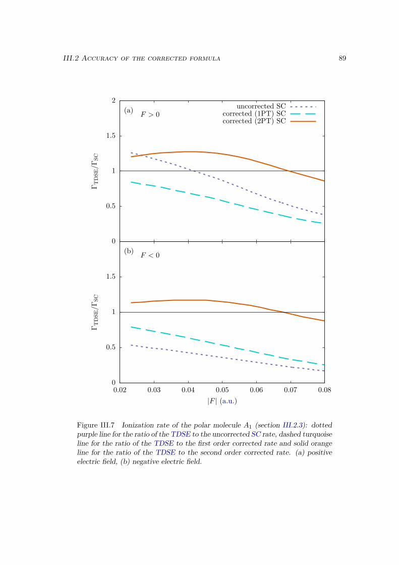
III.2 Accuracy of the corrected formula 89
0
0.5
1
1.5
2(a)
F > 0
0
0.5
1
1.5
0.02 0.03 0.04 0.05 0.06 0.07 0.08
(b)F < 0
Γ TD
SE/Γ S
C
uncorrected SCcorrected (1PT) SCcorrected (2PT) SC
Γ TD
SE/Γ S
C
|F | (a.u.)
Figure III.7 Ionization rate of the polar molecule A1 (section III.2.3): dottedpurple line for the ratio of the TDSE to the uncorrected SC rate, dashed turquoiseline for the ratio of the TDSE to the first order corrected rate and solid orangeline for the ratio of the TDSE to the second order corrected rate. (a) positiveelectric field, (b) negative electric field.
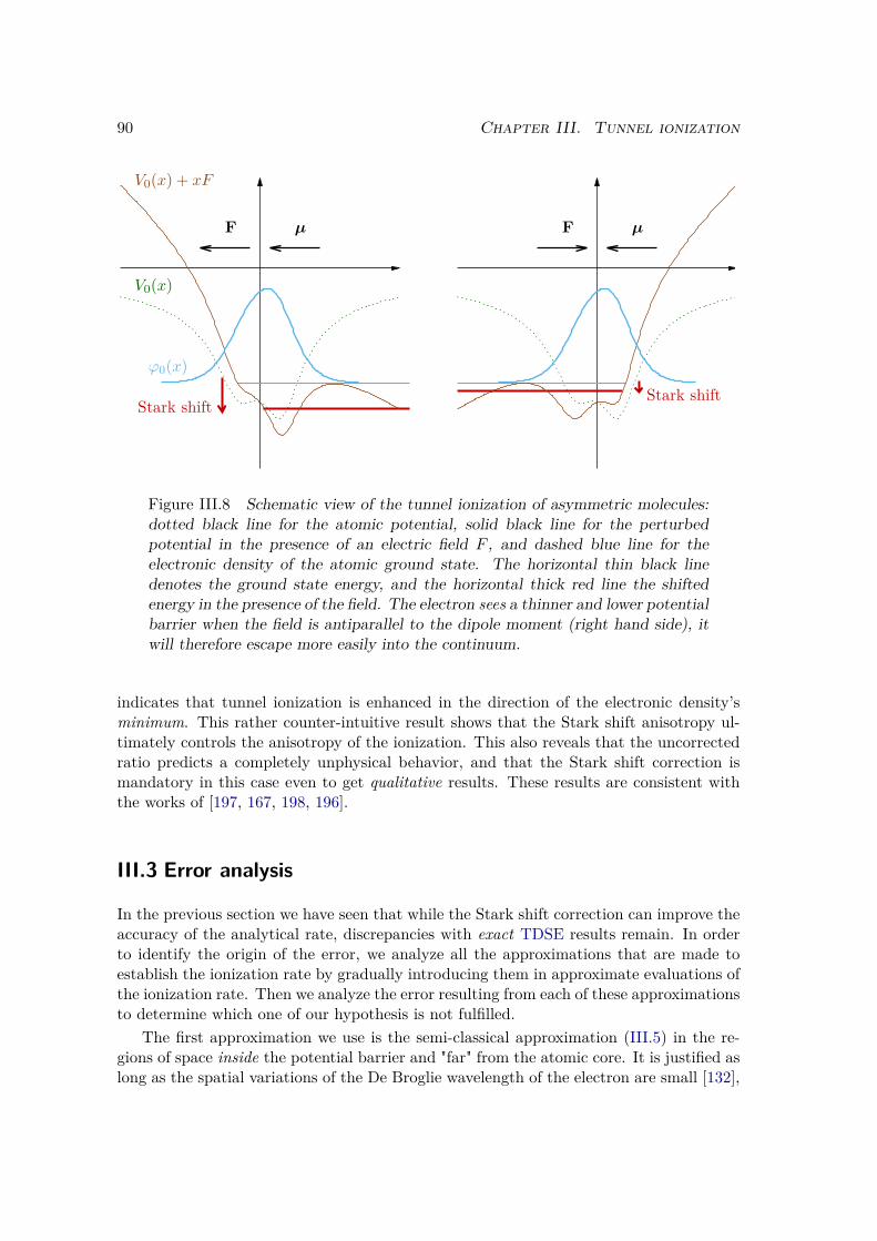
90 Chapter III. Tunnel ionization
Stark shift
µF
ϕ0(x)
V0(x) + xF
V0(x)
Stark shift
µF
Figure III.8 Schematic view of the tunnel ionization of asymmetric molecules:dotted black line for the atomic potential, solid black line for the perturbedpotential in the presence of an electric field F , and dashed blue line for theelectronic density of the atomic ground state. The horizontal thin black linedenotes the ground state energy, and the horizontal thick red line the shiftedenergy in the presence of the field. The electron sees a thinner and lower potentialbarrier when the field is antiparallel to the dipole moment (right hand side), itwill therefore escape more easily into the continuum.
indicates that tunnel ionization is enhanced in the direction of the electronic density’sminimum. This rather counter-intuitive result shows that the Stark shift anisotropy ul-timately controls the anisotropy of the ionization. This also reveals that the uncorrectedratio predicts a completely unphysical behavior, and that the Stark shift correction ismandatory in this case even to get qualitative results. These results are consistent withthe works of [197, 167, 198, 196].
III.3 Error analysis
In the previous section we have seen that while the Stark shift correction can improve theaccuracy of the analytical rate, discrepancies with exact TDSE results remain. In orderto identify the origin of the error, we analyze all the approximations that are made toestablish the ionization rate by gradually introducing them in approximate evaluations ofthe ionization rate. Then we analyze the error resulting from each of these approximationsto determine which one of our hypothesis is not fulfilled.
The first approximation we use is the semi-classical approximation (III.5) in the re-gions of space inside the potential barrier and "far" from the atomic core. It is justified aslong as the spatial variations of the De Broglie wavelength of the electron are small [132],
III.3 Error analysis 91
0.2
0.4
0.6
0.8
1
0.02 0.03 0.04 0.05 0.06 0.07 0.08
Γ −/Γ
+
F (a.u.)
TDSE A1corrected (1PT) SC A1
TDSE A2corrected (1PT) SC A2
Figure III.9 Ionization rate of polar molecular systems. The exact TDSE ratioΓ−/Γ+ is denoted by empty black circles for A1 and by empty black triangles forA2; the corrected analytical ratio given in (III.25) is denoted by a long-dashedturquoise line for A1 and by a short-dashed dark-blue line for A2, the uncorrectedratio given in (III.24) is larger than 1.
which can be written as1|p|2
∣∣∣∣dpdx
∣∣∣∣ 1. (III.26)
If we use only this approximation, we find the following expression for the ionization rate:
Γ1 = |ψ(x0)|2|p(x0)| exp(−2∫ x0
x1|p(x)|dx
), (III.27)
To evaluate the validity of the hypothesis (III.26), the quantity Γ1 is computed numericallyin the case of the atomic system of section III.2.1. For this, the exact wave function ψ(x0)dressed by the field is computed numerically (e.g. by inverse iteration [137] or Runge-Kutta propagation), and then normalized by∫ +∞
x1|ψ(x)|2dx = 1. (III.28)
This choice of normalization is consistent with the way LL and SC build their approximatewave function [132, 184]. Note that it is also consistent with the approximation in equation(36) of [185]. The numerical Γ1 is shown as red connected triangles on Figure III.10 for afield F = 2.5 × 10⁻² a.u., which corresponds to an intensity of 2.2 × 10¹³ W.cm−2. In
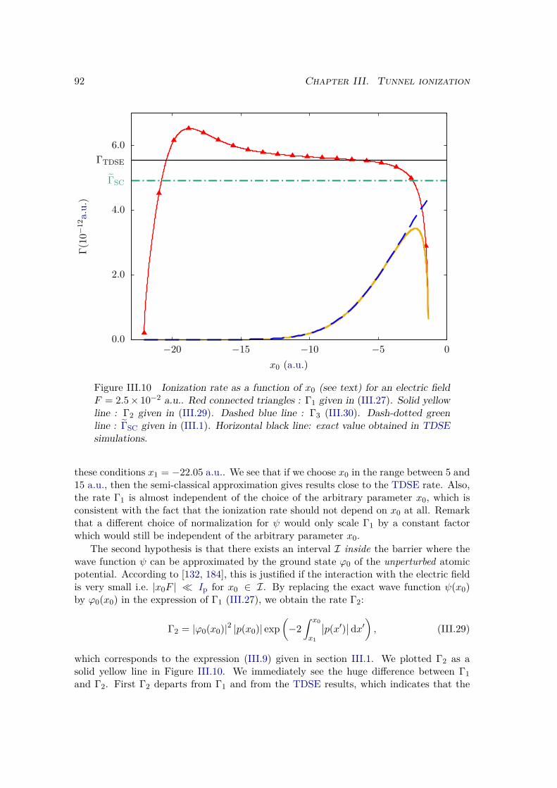
92 Chapter III. Tunnel ionization
0.0
2.0
4.0
6.0
−20 −15 −10 −5 0
ΓTDSE
ΓSC
Γ(10−
12a.
u.)
x0 (a.u.)
Figure III.10 Ionization rate as a function of x0 (see text) for an electric fieldF = 2.5× 10⁻² a.u.. Red connected triangles : Γ1 given in (III.27). Solid yellowline : Γ2 given in (III.29). Dashed blue line : Γ3 (III.30). Dash-dotted greenline : ΓSC given in (III.1). Horizontal black line: exact value obtained in TDSEsimulations.
these conditions x1 = −22.05 a.u.. We see that if we choose x0 in the range between 5 and15 a.u., then the semi-classical approximation gives results close to the TDSE rate. Also,the rate Γ1 is almost independent of the choice of the arbitrary parameter x0, which isconsistent with the fact that the ionization rate should not depend on x0 at all. Remarkthat a different choice of normalization for ψ would only scale Γ1 by a constant factorwhich would still be independent of the arbitrary parameter x0.
The second hypothesis is that there exists an interval I inside the barrier where thewave function ψ can be approximated by the ground state ϕ0 of the unperturbed atomicpotential. According to [132, 184], this is justified if the interaction with the electric fieldis very small i.e. |x0F | Ip for x0 ∈ I. By replacing the exact wave function ψ(x0)by ϕ0(x0) in the expression of Γ1 (III.27), we obtain the rate Γ2:
Γ2 = |ϕ0(x0)|2 |p(x0)| exp(−2∫ x0
x1
∣∣p(x′)∣∣ dx′) , (III.29)
which corresponds to the expression (III.9) given in section III.1. We plotted Γ2 as asolid yellow line in Figure III.10. We immediately see the huge difference between Γ1and Γ2. First Γ2 departs from Γ1 and from the TDSE results, which indicates that the
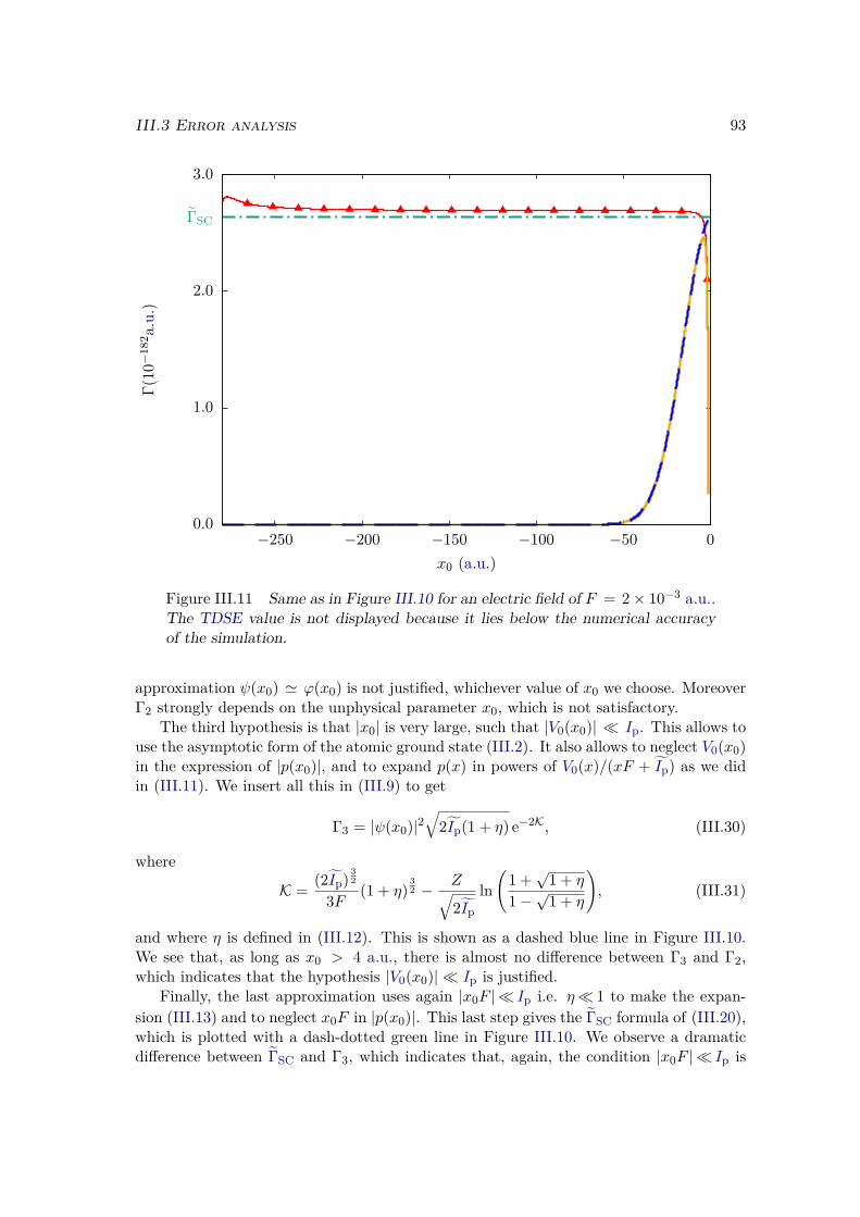
III.3 Error analysis 93
0.0
1.0
2.0
3.0
−250 −200 −150 −100 −50 0
ΓSC
Γ(10−
182 a.u.)
x0 (a.u.)
Figure III.11 Same as in Figure III.10 for an electric field of F = 2× 10⁻³ a.u..The TDSE value is not displayed because it lies below the numerical accuracyof the simulation.
approximation ψ(x0) ' ϕ(x0) is not justified, whichever value of x0 we choose. MoreoverΓ2 strongly depends on the unphysical parameter x0, which is not satisfactory.
The third hypothesis is that |x0| is very large, such that |V0(x0)| Ip. This allows touse the asymptotic form of the atomic ground state (III.2). It also allows to neglect V0(x0)in the expression of |p(x0)|, and to expand p(x) in powers of V0(x)/(xF + Ip) as we didin (III.11). We insert all this in (III.9) to get
Γ3 = |ψ(x0)|2√
2Ip(1 + η) e−2K, (III.30)
where
K = (2Ip) 32
3F (1 + η)32 − Z√
2Ip
ln(
1 +√
1 + η
1−√
1 + η
), (III.31)
and where η is defined in (III.12). This is shown as a dashed blue line in Figure III.10.We see that, as long as x0 > 4 a.u., there is almost no difference between Γ3 and Γ2,which indicates that the hypothesis |V0(x0)| Ip is justified.
Finally, the last approximation uses again |x0F | Ip i.e. η 1 to make the expan-sion (III.13) and to neglect x0F in |p(x0)|. This last step gives the ΓSC formula of (III.20),which is plotted with a dash-dotted green line in Figure III.10. We observe a dramaticdifference between ΓSC and Γ3, which indicates that, again, the condition |x0F | Ip is
94 Chapter III. Tunnel ionization
not fulfilled, whichever value of x0 we consider, for a field of 2.5×10⁻² a.u.. However it isremarkable that the error made by this last approximation almost perfectly compensatesthe error made by the approximation ψ(x0) ' ϕ(x0) so that the SC formula eventuallygives results relatively close to the exact TDSE computations.
We did the same analysis for a much weaker field value F = 2 × 10⁻³ a.u., whichcorresponds to an intensity of 1.4× 10¹¹ W.cm−2. In these conditions x1 = −295.23 a.u..As can be seen in Figure III.11, at this field value the ionization rate is of the orderof magnitude 10−182 a.u. which drastically highlights the extreme non-linearity of theprocess. It is well below any practical application, and obviously below the numericalaccuracy of TDSE simulations, which is why we have no reference TDSE value for thisvalue of F . Nevertheless, this academic case constitutes a severe test of the approximationsrelying on the weak influence of the external field on the electron at the position x0. Wefind that the conclusions concerning the relative roles of the approximations are exactlythe same as the ones obtained with F = 2.5 × 10⁻² a.u.. Indeed, we see in Figure III.11that the two rates Γ1 and Γ2 are very different from one another, and that Γ2 still exhibitsa strong x0 dependency. Therefore the approximation that there exists a point x0 that isat the same time very large, i.e. |V0(x0)| Ip, and very small, i.e. |x0F | Ip, is neverjustified, even for a field value as small as F = 2 × 10⁻³ a.u..
Indeed, for these two condition to be fulfilled at the same time, the electric field hasto be much smaller than the condition one often finds in the literature [184, 174]:
F (2Ip)3/2. (III.32)
For example in the case of hydrogen (Ip = 0.5 a.u.), (2Ip)3/2 = 1 a.u. and the inequal-ity (III.32) is fulfilled for the two field values used in Figure III.10 and Figure III.11.However, the expansion in (III.13) is, in this case, justified if
e−2
3F (1−2|x0|F )3/2 ' e−2
3F e2|x0|, (III.33)
which will hold if the third term of the expansion is negligible, i.e.
e−2|x0|2F ' 1. (III.34)
As we have |x0| 1, we actually need F ≤ 10−4 a.u. for (III.34) to be true. Thismeans that the hypotheses of the Landau and SC derivation are verified if the intensityis below 108 W.cm−2, which corresponds to a meaningless tunnel ionization rate of aboutΓ . 10−2891! However, once again, thanks to the error compensation evidenced with thestronger field as well as with the weaker one (see Figure III.10 and III.11), the Landaurate gives semi-quantitative results for intensities up to 1012 − 1013 W.cm−2. The useof this formula for finite values of the electric field has therefore more empirical thantheoretical foundations.
III.4 ConclusionWe computed the tunnel ionization rate in a static electric field for different symmetricsystems using both the standard analytical formulas and exact numerical solution of theTDSE. By comparing the two approaches we found that the standard rate derived by
III.4 Conclusion 95
Smirnov and Chibisov [184] only yields qualitative trends in the best cases. We demon-strated that we can correct this formula by taking into account the Stark shift, and deriveda consistent formula where the Stark shift correction only appears in the argument of thedominant exponential term. We tested this formula for model systems with differentphysical properties and showed that the correction systematically improves the accuracyof the ionization rate. We proved that if the energy gap between the two first boundstates remains big enough compared to the Stark shift, then second order perturbationtheory is sufficient to compute the Stark shift, implying that one only needs to know thepermanent dipole moment and polarizability of the system under study. However, weshowed that for highly polarizable systems, second order perturbation theory is a verypoor approximation of the Stark shift and therefore a very bad correction of the ionizationrate. In these cases, one has to consider degenerate perturbation theory. Furthermorewe showed that for polar systems the Stark shift is the dominant contribution to theanisotropy of the ionization. It is therefore a central effect to take into account even fora qualitative description of tunnel ionization in molecules.
Finally, the main conclusion of this work is that the hypotheses used for the Landauderivation of the tunnel ionization rate are unjustified at working intensities to modelquantitatively atoms and molecules interacting with strong laser fields. We showed thatthe accuracy of the Landau formula is difficult to predict since it originates from thecompensation of different approximations. Consequently, all the dynamical formulas thatare based on this static rate (ADK), or asymptotically equal to it in the limit of a zerofrequency electric field (e.g. the rate derived by PPT [174]), should be handled with carewhen used for quantitative applications, even though they are very practical.

96 Chapter III. Tunnel ionization
Chapter IV
Two-center interferences in high orderharmonic generation
We saw that HHG has two aspects that give rise to very different types of experiments: itcan be used either as a light source, or as a self-probe spectroscopic tool. In this chapter weconcentrate on the latter, i.e. how we can extract information about the emitting systemfrom the HHG spectrum. In particular, we consider homonuclear diatomic molecules.For such systems, we have seen in Chapter I.3 that the third and last step of the HHGprocess, namely the recombination step, may occur at any one of the two nuclei. Thetwo centers of the molecule can therefore be seen as two coherent point sources. Exactlylike Young’s two slits, they can interfere constructively or destructively depending on thefrequency of the emitted harmonic, and on the distance between the two centers. Theseinterferences encode the structure of the molecule, and more precisely the structure ofthe orbitals that participate to the HHG process [200, 128, 201, 202].
Obviously, to efficiently retrieve this structural information from the HHG spectrum,we need accurate theoretical models. This remains a challenge since the direct solutionof the TDSE is numerically too costly for such systems, so that SFA models are in gen-eral used to explain and interpret interference features in molecules. We have seen inChapter I.3 that in the SFA framework the HHG spectrum is directly proportional tothe recombination dipole. This quantity contains a lot of information on the emittingsystem. In particular for diatomic molecules it exhibits a zero at a particular energywhich depends on the internuclear distance. This zero is a manifestation of the destruc-tive two-center interference, and directly appears as a minimum in the HHG spectrumtogether with a jump of ±π of the harmonics phase. With the recent advances that allowto align an ensemble of molecules, this minimum has been experimentally observed inseveral systems such as CO2 [203–208], N2O [99, 209] and N2 [210].
Although the standard version of the SFA that we have derived in section I.3.3 is ableto predict such a minimum and phase jump, it has several drawbacks. As we will seein the following, because of the plane wave approximation, the position of this minimumis in agreement neither with experiments nor with direct solutions of the TDSE. Moreimportantly the standard SFA predicts a peaked minimum along with a very sharp phasejump, whereas in experiments [204, 205, 99, 209] and in TDSE simulations [211, 200, 212],the minimum and the phase jump are smoothed over several harmonics. This smoothing
97
98 Chapter IV. Two-center interferences in HHG
was attributed to a dressing of the ionized orbital by the instantaneous electric field[213–215].
To overcome the limitations of the atomic model, Chirilă and Lein [84] developed anew approach, called molecular SFA which incorporate the molecular structure, within theLCAO approximation, into the search of saddle points (as we have seen in section I.3.3 d)).This model was then intensively investigated by Figueira de Morisson Faria [128] whofocused on the position and shape of the minimum, and by François Risoud during his PhDin our group (2013-2016) [129, 157] who also considered the position and shape of the phasejump for 1D systems considered as aligned molecules. We also derived a comprehensiveanalytical model by expanding the molecular SFA close to the atomic solution. Thisexpansion allowed to give a direct interpretation of the smoothing of the phase jump,and to give precise conditions to observe a sharp jump: when the recombination timeof the harmonic corresponding to the jump coincides with a zero of the laser electricfield. However, this derivation was incomplete since the saddle point prefactor expression(see (I.109)) was not obtained, so that discrepancies between the expansion and the totalmolecular SFA remained. The sharp jump was actually observed for a recombinationcorresponding to a small but non zero value of the field. Besides, the derivation was onlyperformed for molecules aligned in the direction of the field polarization.
In this work we complete the analytical work performed by François Risoud [129], andfind the expression of the "ζ constant" which was mentioned in [157]. We also extendthe study to two dimensional systems. In particular we investigate the influence of theorientation of the molecule with respect to the field, and we question the commonlyaccepted idea that the 2-center interference only depends on the orientation through acos θ factor. Finally we search for the origin of the observed discrepancies in the predictionof the minimum position. To this end, we compare the accuracy of the PWA and of theLCAO approximation, and we test the accuracy of the Ip correction that was proposedto improve the PWA.
Objectives
ü Complete the analytical work of François Risoud: define without ambiguity theparameter of the expansion and find the expression of the prefactor.
ü Investigate the effect of the orientation of the molecule with respect to the field.
ü Find the limiting approximations at the origin of the discrepancies.
IV.1 Analytic expansion of the molecular SFA
We first derive the important expressions in sections IV.1.1 and IV.1.2 and then discussthese results in section IV.1.3.
IV.1.1 Molecular saddle point equations
We recall here the molecular saddle point equations as obtained in section I.3.3 d):
IV.1 Analytic expansion of the molecular SFA 99
∫ t
t′[p + AL(τ)] dτ +
[(−1)α − (−1)β
] R2 = 0 (IV.1a)
[p + AL(t)]22 + Ip − ω + (−1)βFL(t) · R
2 = 0 (IV.1b)
[p + AL(t′)]22 + Ip + (−1)αFL(t′) · R
2 = 0 (IV.1c)
where p is the electron momentum, t the recombination time, t′ the ionization time, ALthe vector potential of the laser, and α, β label the nuclei of the molecule at which theelectron is ionized and recombines, respectively.
We note that these equations are actually very similar to the atomic saddle pointequations (I.104), but with additional terms that are proportional to R. If we considerthat these terms only induce a small perturbation to the original saddle point equations,we may actually expand the solutions of these equations in powers of R. We assumethat the field is polarized along the x axis, and that R belongs to the xy plane, withcomponents Rx and Ry. We can thus rewrite the system of equations as
∫ t
t′[px +AL(τ)] dτ +
[(−1)α − (−1)β
] Rx2 = 0 (IV.2a)
py(t− t′) +[(−1)α − (−1)β
] Ry2 = 0 (IV.2b)
pz(t− t′) = 0 (IV.2c)[p + AL(t)]2
2 + Ip − ω + (−1)βFL(t)Rx2 = 0 (IV.2d)
[p + AL(t′)]22 + Ip + (−1)αFL(t′)Rx2 = 0 (IV.2e)
and expand its solutions in powers of R:
pxαβ = pat +Rx∂xpxαβ +Ry∂yp
xαβ +O(R2) (IV.3a)
pyαβ = Rx∂xpyαβ +Ry∂yp
yαβ +O(R2) (IV.3b)
tαβ = tat +Rx∂xtαβ +Ry∂ytαβ +O(R2) (IV.3c)t′αβ = t′at +Rx∂xt
′αβ +Ry∂yt
′αβ +O(R2) (IV.3d)
where we noted ∂i the partial derivatives with respect to Ri taken at R = 0, and wherewe used the subscript "at" to denote the solutions of the atomic saddle point equations,i.e. where R = 0. Note that these equations have no solution verifying t = t′, so thatwe always have pzαβ = 0. In the atomic case, we also have pyat = 0, i.e. the stationarymomentum pat is parallel to the field polarization direction x. When we put this firstorder expansion in the saddle point equations (IV.3), we obtain a linear set of equations
100 Chapter IV. Two-center interferences in HHG
for the first order derivatives :
0 = [pat +AL(tat)] ∂xtαβ −[pat +AL(t′at)
]∂xt′αβ + (tat − t′at)∂xpxαβ + (−1)α − (−1)β
2(IV.4a)
0 =− [pat +AL(tat)]FL(tat)∂xtαβ + [pat +AL(tat)] ∂xpxαβ + (−1)β2 FL(tat) (IV.4b)
0 =−[pat +AL(t′at)
]FL(t′at)∂xt′αβ +
[pat +AL(t′at)
]∂xp
xαβ + (−1)α
2 FL(t′at) (IV.4c)
0 = [pat +AL(tat)] ∂ytαβ −[pat +AL(t′at)
]∂yt′αβ + (tat − t′at)∂ypxαβ (IV.4d)
0 =− [pat +AL(tat)]FL(tat)∂ytαβ + [pat +AL(tat)] ∂ypxαβ (IV.4e)0 =−
[pat +AL(t′at)
]FL(t′at)∂yt′αβ +
[pat +AL(t′at)
]∂yp
xαβ (IV.4f)
0 =(tat − t′at)∂xpyαβ (IV.4g)
0 =(tat − t′at)∂ypyαβ + (−1)α − (−1)β
2 (IV.4h)
From (IV.4g) we directly find that ∂xpyαβ = 0, and from (IV.4h) we have:
∂ypyαβ = (−1)β − (−1)α
2(tat − t′at), (IV.5)
which leads to the final first order expression of the y component of the stationary mo-mentum:
pyαβ = (−1)β − (−1)α2(tat − t′at)
Ry
(IV.6)
We conclude that, at first order, the trajectories where the electron is ionized at onecenter and recombines with the same center have a stationary momentum with a zero ycomponent. This is actually quite intuitive since such trajectories behave similarly to theatomic ones. On the contrary, for the trajectories where the electron is ionized at onecenter and recombines with the other center, which are specific of the molecular case, thestationary momentum has a non zero y component.
From (IV.4a), (IV.4b), and (IV.4c), we get[FL(t′at) [pat +AL(tat)]− FL(tat)
[pat +AL(t′at)
]+ FL(tat)FL(t′at)(tat − t′at)
]∂xp
xαβ = 0.
(IV.7)We thus find that ∂xpxαβ = 0 is one solution of the system of equations. It will be theonly solution if
∆ = FL(t′at) [pat +AL(tat)]−FL(tat)[pat +AL(t′at)
]+FL(tat)FL(t′at)(tat−t′at) 6= 0. (IV.8)
This term ∆ is simply the determinant of the subsystem of equations (IV.4a,IV.4b,IV.4c).We checked numerically that it indeed does not vanish. From (IV.4d), (IV.4e), and (IV.4f),we obtain exactly the same equation for ∂ypxαβ. We thus find that the x component of
IV.1 Analytic expansion of the molecular SFA 101
the stationary moment is equal to the atomic one at first order:
pxαβ = pat(IV.9)
By inserting this in (IV.4b), (IV.4c), (IV.4e) and (IV.4f) we easily find the first orderexpression of tαβ and t′αβ:
tαβ = tat + (−1)βRx2 [pat +AL(tat)]
t′αβ = t′at + (−1)αRx2 [pat +AL(t′at)]
(IV.10)
(IV.11)
These two expressions have a clear physical interpretation, as was pointed out in [129].They indicate that the molecular ionization and recombination times comprise an addi-tional delay compared to their atomic equivalent. This delay is equal to the time it takesfor the electron to travel half the molecule size, which corresponds to the distance betweenthe center of mass of the molecule and the nucleus at which the electron is ionized or atwhich it recombines. Note that since [pat +AL(tat)]2 > 0, this molecular recombinationtime delay is real, while since [pat +AL(t′at)]
2 < 0, the molecular ionization time delayis purely imaginary. This is related to the fact that tunnel ionization has no classicalequivalent.
We want to insist here on an issue that was not mentioned in [129]: these moleculartime delays should only appear for trajectories where the electron is ionized at one centerand recombines with the other center. For the atomic-like trajectories, that start at onecenter and end at the same center, we should not see any difference with the atomic case.Indeed, the effect of the molecular potential is neglected as soon as the electron is ionized,so that these trajectories should behave exactly like the atomic ones. This inconsistency isa direct consequence of the fact that the SFA framework is not translationally invariant.As was pointed out in [128], this can be tackled in the atomic case by choosing the originat the position of the nucleus. However this cannot be done for both nuclei at the sametime in the molecular case, hence this incoherence.
IV.1.2 HHG spectrumIn the molecular SFA model (see section I.3.3 d)) the HHG spectrum is proportional tothe average value of the dipole which is given by
Dα,β(ω) =2∑
α,β=1Cα,β(tαβ, t′αβ)L
(pαβ + AL(tαβ)
)Mα
(pαβ + AL(t′αβ), t′αβ
)e−iSα,β ,
(IV.12)where Sα,β is the modified action defined in (I.119), Mα is the molecular ionizationdipole defined in (I.113), L is the molecular recombination dipole (I.115) and Cα,β isthe molecular prefactor defined in (I.109). To get the first order expansion of the dipoleexpression, we first expand separately Sα,β, Mα, L and Cα,β.
102 Chapter IV. Two-center interferences in HHG
a) Semi-classical action
The modified semi classical action reads
Sα,β(pαβ, tαβ, t′αβ) =∫ tαβ
t′αβ
dτ(
[pαβ + AL(τ)]2
2 + Ip
)− ωtαβ
+ (−1)α[pαβ + AL(t′αβ)
]· R
2− (−1)β [pαβ + AL(tαβ)] · R
2
(IV.13)
which can be expanded as
Sα,β(pαβ, tαβ, t′αβ) =∫ tat
t′at
dτ(
[pat + AL(τ)]2
2 + Ip
)− ωtat
+
[
[pat + AL(tat)]22 + Ip − ω
]Rx∂xtαβ
−
[
[pat + AL(t′at)]22 + Ip
]Rx∂xt
′αβ
+ (−1)α[pat + AL(t′at)
]· R
2− (−1)β [pat + AL(tat)] ·
R2 +O(R2),
(IV.14)
where we recognized the atomic saddle point equations (I.104b) and (I.104c), and usedthem to simplify the expression of the action. We finally get
Sα,β(pαβ, tαβ, t′αβ) = Sat + (−1)α[pat +AL(t′at)
] Rx2 − (−1)β [pat +AL(tat)]
Rx2 +O(R2)
,(IV.15)
where Sat is the atomic action (I.108).
b) Ionization dipole
The molecular ionization dipole reads
Mα
(pαβ + AL(t′αβ), t′αβ
)= −
FL(t′αβ)√2(1 + w(R)
)[i∂φa∂px
(pαβ + AL(t′αβ)
)
+ (−1)αRx2 φa(pαβ + AL(t′αβ)
)].
(IV.16)
The overlap w(R) is obviously an even function of R, so that the first order term vanishesand we simply get
w(R) = 1 +O(R2).(IV.17)
IV.1 Analytic expansion of the molecular SFA 103
The ionization dipole thus expands as
Mα
(pαβ + AL(t′αβ), t′αβ
)=Mat
(pat + AL(t′at), t′at
)+ (−1)αRx
2 MX
(pat + AL(t′at), t′at
)+ [(−1)β − (−1)α]Ry
2 MY
(pat + AL(t′at), t′at
)+O(R2),
(IV.18)where
Mat(p, t′) = −iFL(t′)2
∂φa∂px
(p), (IV.19)
and where we defined
MX(p, t′) = −FL(t′)2 φa(p)− iωL
2AL(t′)2px
∂φa∂px
(p) + iFL(t′)2
2px∂2φa∂p2
x
(p) (IV.20)
MY (p, t′) = −i FL(t′at)2(tat − t′at)
∂2φa∂px∂py
(pat + AL(t′at)
)(IV.21)
c) Recombination dipole
The molecular recombination dipole writes
L(pαβ + AL(tαβ)
)= pαβ + AL(tαβ)√
2(1 + w(R)
) φa(pαβ + AL(tαβ)
). (IV.22)
We mainly concentrate on its component along the direction of the laser field polarization,i.e. the x direction, which expands as
Lx(pαβ + AL(tαβ)
)=Lat
(pat + AL(tat)
)+ (−1β)Rx
2 LX(pat + AL(tat), tat
)+ [(−1)β − (−1)α]Ry
2 LY(pat + AL(tat), tat
)+O(R2),
(IV.23)
104 Chapter IV. Two-center interferences in HHG
whereLat(p) = px
2 φa(p), (IV.24)
and where
LX(p, t) = −FL(tat)2px
φa(p)− FL(tat)2
∂φa∂px
(p) (IV.25)
LY (p, t) = − px2(tat − t′at)
∂φa∂py
(p). (IV.26)
For the sake of exhaustivity, we also give here the expansion of the y component of themolecular recombination dipole:
Ly(pαβ + AL(tαβ)
)= [(−1)β − (−1)α]Ry
4(tat − t′at)φa(pat + AL(tat)
)+O(R2).
(IV.27)
d) Saddle point prefactor
The first order expansion of the saddle point prefactor was not obtained in [129], whereits influence was only assessed numerically. I present here its derivation.
The saddle point prefactor expression reads
Cαβ(tαβ, t′αβ) =(
2πi(tαβ − t′αβ)
) 32 π√
detHS
(p)αβ
(tαβ, t′αβ), (IV.28)
where HS
(p)αβ
is the Hessian matrix of S(p)αβ (t, t′) = Sαβ(pαβ(t, t′), t, t′), with pαβ(t, t′) the
solution of (IV.1a):
detHS
(p)αβ
(tαβ, t′αβ) =∂2S
(p)αβ
∂t2∂2S
(p)αβ
∂t′2−∂2S
(p)αβ
∂t∂t′
2
. (IV.29)
Using the chain rule for computing the derivative of this composition of functions, we find
∂2S(p)αβ
∂t2(t, t′) = −FL(t) · [pαβ + AL(t)]− [pαβ + AL(t)]2
t− t′+ (−1)βRx
2 ω2LAL(t) (IV.30)
∂2S(p)αβ
∂t′2(t, t′) = FL(t′) · [pαβ + AL(t′)]− [pαβ + AL(t′)]2
t− t′− (−1)αRx
2 ω2LAL(t′) (IV.31)
∂2S(p)αβ
∂t∂t′(t, t′) = [pαβ + AL(t)] · [pαβ + AL(t′)]
t− t′. (IV.32)
IV.1 Analytic expansion of the molecular SFA 105
We can thus expand the Hessian determinant as:
detHS
(p)αβ
(tαβ, t′αβ) = detHS
(p)at
(tat, t′at)
1− Rx2
[(−1)αFL(t′at)
[pat +AL(t′at)]2 + (−1)βFL(tat)
[pat +AL(tat)]2
− (−1)α(tat − t′at) [pat +AL(t′at)]
+ (−1)β(tat − t′at) [pat +AL(tat)]
]+O(R2). (IV.33)
We finally get
Cαβ(tαβ, t′αβ) = Cat(tat, t′at)
1 + Rx2
[(−1)αFL(t′at)
2 [pat +AL(t′at)]2
+ (−1)βFL(tat)2 [pat +AL(tat)]2
+ (−1)α(tat − t′at) [pat +AL(t′at)]
− (−1)β(tat − t′at) [pat +AL(tat)]
]+O(R2).
(IV.34)
e) Sum over electronic trajectories
Since the HHG emitted light is dominantly polarized along the field polarization direction,we will concentrate on the x component of the dipole Dα,β. To compute its expression,we put back together the four expressions in (IV.15), (IV.18), (IV.23) and (IV.34) andsum over α and β, i.e. over the four electronic trajectories. We get an expression thatcan organized as:
D(x)(ω) = −ωCat
[D(pat, tat, t
′at) +Rydmix(pat, tat, t
′at)]e−iSat ,
(IV.35)
where the term D is equal at first order to the factored expression:
D(pat, tat, t′at)
1st order= drec
(pat +AL(tat), tat, t
′at
)dion
(pat +AL(t′at), tat, t
′at
), (IV.36)
106 Chapter IV. Two-center interferences in HHG
where
drec(p, t, t′) =pxφa(p) cos(p ·R
2
)
− iRx2
[FL(t)∂φa
∂px(p) + FL(t)
2pxφa(p) + 1
t− t′φa(p)
]sin(p ·R
2
)(IV.37)
dion(p, t, t′) =− iFL(t′)∂φa∂px
(p) cos(p ·R
2
)
− iRx2
− FL(t′)φa(p) + iFL(t′)2
px
∂2φa∂p2
x
(p)
+ i∂φa∂px
(p)[− 3
2(t− t′)px+ FL(t′)
4Ip− ωL
2AL(t′)px
]sin(p ·R
2
)(IV.38)
dmix(p, t, t′) =[p + AL(t)] · FL(t′)2(t− t′) sin
[(2p + AL(t) + AL(t′)
)· R
2
]
×[∂φa∂px
(p + AL(t′)
)∂φa∂py
(p + AL(t)
)+ φa
(p + AL(t)
)∂2φa∂px∂py
(p + AL(t′)
)].
(IV.39)
IV.1.3 DiscussionWe will first comment the case of a molecule that is aligned with the laser polarizationdirection, here x. In this case Ry = 0, and the above expression (IV.35) is at first ordervery similar to the one obtained in [129]:
D(x)(ω) = −ωCatdrec
(pat +AL(tat), tat, t
′at
)dion
(pat +AL(t′at), tat, t
′at
)e−iSat , (IV.40)
but where the formulas for the modified ionization dion and recombination drec dipolesare slightly different because of the saddle point prefactor contribution that was neglectedin [129]. Remind that the HHG spectrum is proportional to the dipole D(x), so we willdiscuss this quantity D(x) as if it were directly the HHG spectrum. It is obviously a misuseof language, but I think it simplifies the discussion.
From this factored form (IV.40) it is straightforward to see that a zero of drec or dionwill result in a sharp minimum in the HHG power spectrum. As already predicted in[200] and detailed in [129], the ionization dipole has little influence, and the minimumin the spectrum is actually caused by a zero of the recombination dipole. This can beunderstood by looking at the argument in dion, i.e. pat+AL(t′at), which, as can be deducedfrom (I.104c), is simply equal to ±i
√2Ip and thus does not depend on the frequency of the
emitted harmonic. The ionization dipole depends on the harmonic frequency, and thusinfluences the HHG spectrum, only through terms that do not contain any structuralinformation on the molecule, i.e. FL(t′at), AL(t′at), and (tat − (t′at)).
On the contrary, the argument in drec is pat +AL(tat) = ±√
2(ω − Ip) (using (I.104b))where ω is the frequency of the emitted harmonic. If the modified recombination dipole
IV.1 Analytic expansion of the molecular SFA 107
drec displays a zero at pmin, the HHG spectrum will thus exhibit a sharp minimum atthe harmonic frequency ωmin = Ip + [pmin + AL(tat)]2/2. In the model developped byLein [200], this zero coincides with the zero of the unmodified recombination dipole drec(I.114), and thus occurs at [pmin + AL(tat)] ·R/2 = (2q + 1)π/2, where q is an integer.This creates a minimum in the spectrum at
ωmin = Ip + (π + 2qπ)2
2R2 , q ∈ Z. (IV.41)
This is the formula that is generally used to predict the position of the minimum in theHHG spectrum [216–219]1.
This value of pmin predicted by Lein actually corresponds to a zero of the cosine termin the expression of drec (IV.37). However the second term of the expression, proportionalto the sine function, does not vanish at p = pmin. As was thoroughly investigated byFrançois Risoud [129, 157], this pmin thus does not correspond to a zero of the modifiedrecombination dipole drec, but to a smoothed minimum. Nevertheless, there are somecircumstances where both terms may cancel simultaneously, leading to a zero of the totalmodified recombination dipole, hence to a sharp minimum in the HHG spectrum. Fromthe expression of drec (IV.37), we see that this will occur when both the cosine function(IV.42), and the term in factor of the sine function (IV.43) vanishes:
[pat +AL(tat)]R
2 = π
2 + qπ, q ∈ Z (IV.42)
FL(tat)∂φa∂px
(pat + AL(tat)
)+ FL(tat)
2 [pat +AL(tat)]φa
(pat + AL(tat)
)+ 1tat − t′at
φa
(pat + AL(tat)
)= 0. (IV.43)
As explained in [129, 157] the position of the minimum is defined by the zero of thecosine function, i.e. by equation (IV.42), and thus only depends on R. The shape of theminimum is determined by the left hand side of (IV.43): if this term cancels then theminimum is sharp, otherwise it is smoothed. Note that this second condition depends onthe laser intensity and frequency, but also on the considered electronic trajectory: indeed,both the short and long trajectories display a minimum at the same harmonic frequency- however this minimum may be smoothed for one type of trajectories, and sharp for theother. To observe the minimum in the spectrum, it is thus advantageous to separate thecontributions of the two types of trajectories, as was done in [129, 157].
We draw the attention of the reader to the fact that we obtained a condition (IV.43)for the sharpness of the minimum which is in disagreement with the one given by FrançoisRisoud. In [129], because the saddle point prefactor contribution was neglected, the con-dition that was obtained was similar to (IV.43) but without the third term. The equationthus reduced to FL(tat) = 0 which was not in agreement with numerical simulations.To tackle the problem a constant ζ was empirically added to the expression. We findthis is actually not a constant but depends on the saddle point solution, and thus on the
1Actually, in the formula used by [216, 217] the continuum energies are shifted by an amount of Ip.This is supposed to compensate for the PWA by taking into account the effect of the potential on thecontinuum states. We will come back on this correction in section IV.2.3.
108 Chapter IV. Two-center interferences in HHG
intensity and wavelength of the laser. Our findings explain why the minimum was foundto be sharp in conditions where FL(tat) 6= 0 [129], and settle the disparity between thenumerical and analytical predictions.
In the case where the molecule is not aligned with the laser polarization direction,we have an additional term, proportional to Ry = R sin θ, in the expression of thedipole D(x) (IV.35). Because of this term, the expression can no longer be factoredout as we did in the aligned case (IV.40). Consequently the zeros of drec may not nec-essarily correspond to minima of the HHG spectrum. This is actually in contradictionwith the commonly accepted idea that the aligned and the non-aligned case would beequivalent problems, and that to go from the former to the latter, one would only haveto replace R by Rx = R cos θ, θ being the angle between the molecule and the electricfield [200, 129]. Unfortunately we did not have time to assess analytically the influence ofthis dmix term. We will thus try to understand the influence of the molecular orientationthrough numerical simulations in the next section.
IV.2 Numerical simulations
In this section we investigate the accuracy of the molecular SFA model by confronting itspredictions to 1D and 2D numerical simulations.
IV.2.1 Methods
We consider a 2D system analogous to the 1D system used in [129, 157] where the electronis trapped in a two center Soft-Coulomb potential:
V (r) = − 1/2√a2 + (r + R/2)2
− 1/2√a2 + (r−R/2)2
. (IV.44)
This is a simple benchmark model for diatomic molecules. As in [129, 157], the parametera is optimized at each value of R to keep the ionization potential of the system constantand equal to the ionization potential of the H2 molecule Ip(R) = 0.567 a.u. = 15.43 eV.This allows to forget the Ip dependency of the position and shape of the interference,and thus to concentrate on the contribution of the internuclear distance R, molecularorientation θ and laser intensity IL.
We also consider a system that is designed to be "intermediary" between the 1D andthe 2D case. In this case the electron is trapped in an asymmetric potential, which writes,in a frame where the molecule is aligned along the x axis:
Vκ(r) = − 1/2√a2 + (x+R/2)2 + κy2
− 1/2√a2 + (x−R/2)2 + κy2
, (IV.45)
where the parameter κ is smaller than 1 a.u., so that the potential wells are wider inthe direction perpendicular to the molecular axis, i.e. the y direction. As a result themomentum of the electron is more confined in the y direction, and the electron behavessimilarly to a 1D system.
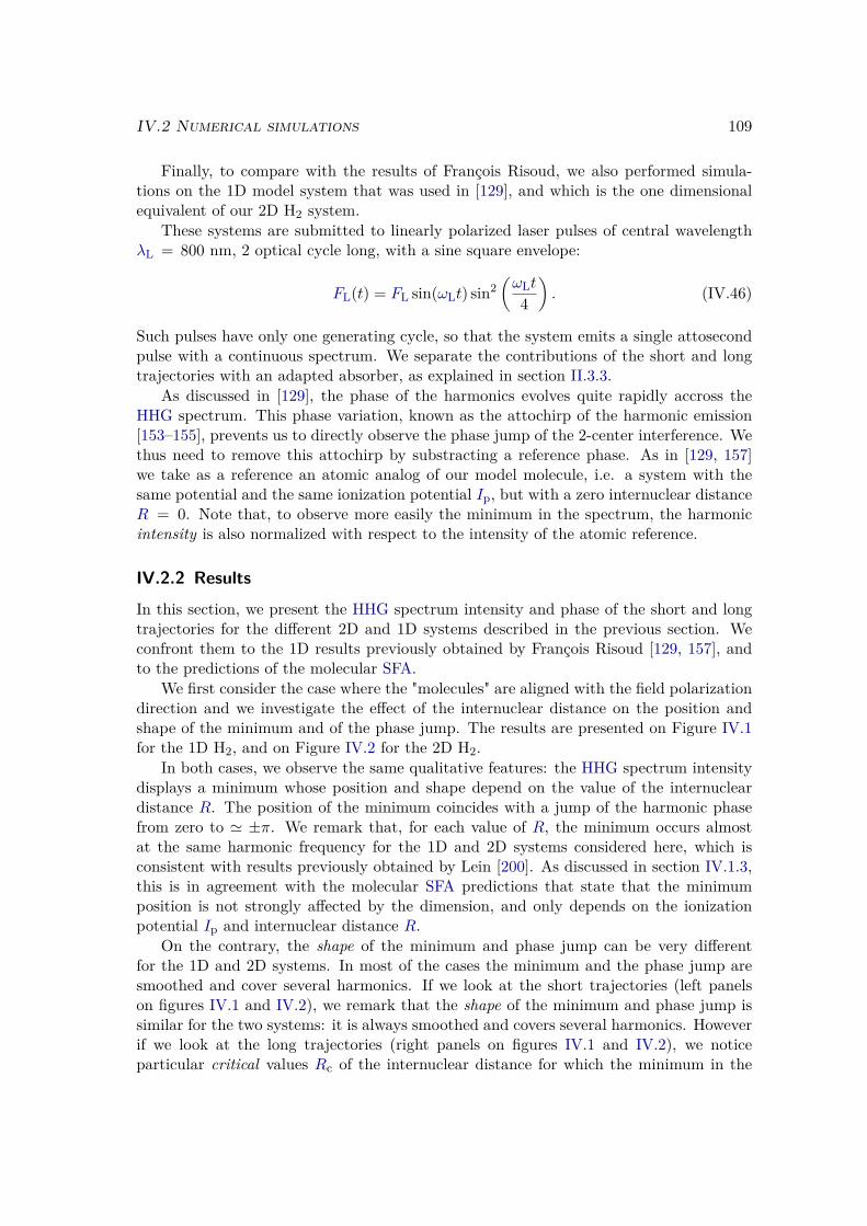
IV.2 Numerical simulations 109
Finally, to compare with the results of François Risoud, we also performed simula-tions on the 1D model system that was used in [129], and which is the one dimensionalequivalent of our 2D H2 system.
These systems are submitted to linearly polarized laser pulses of central wavelengthλL = 800 nm, 2 optical cycle long, with a sine square envelope:
FL(t) = FL sin(ωLt) sin2(ωLt
4
). (IV.46)
Such pulses have only one generating cycle, so that the system emits a single attosecondpulse with a continuous spectrum. We separate the contributions of the short and longtrajectories with an adapted absorber, as explained in section II.3.3.
As discussed in [129], the phase of the harmonics evolves quite rapidly accross theHHG spectrum. This phase variation, known as the attochirp of the harmonic emission[153–155], prevents us to directly observe the phase jump of the 2-center interference. Wethus need to remove this attochirp by substracting a reference phase. As in [129, 157]we take as a reference an atomic analog of our model molecule, i.e. a system with thesame potential and the same ionization potential Ip, but with a zero internuclear distanceR = 0. Note that, to observe more easily the minimum in the spectrum, the harmonicintensity is also normalized with respect to the intensity of the atomic reference.
IV.2.2 Results
In this section, we present the HHG spectrum intensity and phase of the short and longtrajectories for the different 2D and 1D systems described in the previous section. Weconfront them to the 1D results previously obtained by François Risoud [129, 157], andto the predictions of the molecular SFA.
We first consider the case where the "molecules" are aligned with the field polarizationdirection and we investigate the effect of the internuclear distance on the position andshape of the minimum and of the phase jump. The results are presented on Figure IV.1for the 1D H2, and on Figure IV.2 for the 2D H2.
In both cases, we observe the same qualitative features: the HHG spectrum intensitydisplays a minimum whose position and shape depend on the value of the internucleardistance R. The position of the minimum coincides with a jump of the harmonic phasefrom zero to ' ±π. We remark that, for each value of R, the minimum occurs almostat the same harmonic frequency for the 1D and 2D systems considered here, which isconsistent with results previously obtained by Lein [200]. As discussed in section IV.1.3,this is in agreement with the molecular SFA predictions that state that the minimumposition is not strongly affected by the dimension, and only depends on the ionizationpotential Ip and internuclear distance R.
On the contrary, the shape of the minimum and phase jump can be very differentfor the 1D and 2D systems. In most of the cases the minimum and the phase jump aresmoothed and cover several harmonics. If we look at the short trajectories (left panelson figures IV.1 and IV.2), we remark that the shape of the minimum and phase jump issimilar for the two systems: it is always smoothed and covers several harmonics. Howeverif we look at the long trajectories (right panels on figures IV.1 and IV.2), we noticeparticular critical values Rc of the internuclear distance for which the minimum in the
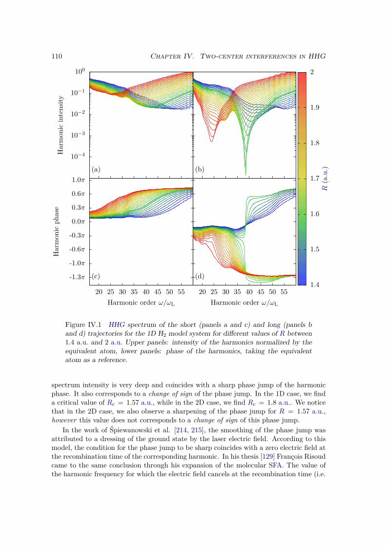
110 Chapter IV. Two-center interferences in HHG
10−4
10−3
10−2
10−1
100
(a) (b)
-1.3π
-1.0π
-0.6π
-0.3π
0.0π
0.3π
0.6π
1.0π
20 25 30 35 40 45 50 55
(c)
20 25 30 35 40 45 50 55
(d)
Harmon
icintensity
Harmon
icph
ase
Harmonic order ω/ωL Harmonic order ω/ωL
1.4
1.5
1.6
1.7
1.8
1.9
2
R(a.u.)
Figure IV.1 HHG spectrum of the short (panels a and c) and long (panels band d) trajectories for the 1D H2 model system for different values of R between1.4 a.u. and 2 a.u. Upper panels: intensity of the harmonics normalized by theequivalent atom, lower panels: phase of the harmonics, taking the equivalentatom as a reference.
spectrum intensity is very deep and coincides with a sharp phase jump of the harmonicphase. It also corresponds to a change of sign of the phase jump. In the 1D case, we finda critical value of Rc = 1.57 a.u., while in the 2D case, we find Rc = 1.8 a.u.. We noticethat in the 2D case, we also observe a sharpening of the phase jump for R = 1.57 a.u.,however this value does not corresponds to a change of sign of this phase jump.
In the work of Śpiewanowski et al. [214, 215], the smoothing of the phase jump wasattributed to a dressing of the ground state by the laser electric field. According to thismodel, the condition for the phase jump to be sharp coincides with a zero electric field atthe recombination time of the corresponding harmonic. In his thesis [129] François Risoudcame to the same conclusion through his expansion of the molecular SFA. The value ofthe harmonic frequency for which the electric field cancels at the recombination time (i.e.
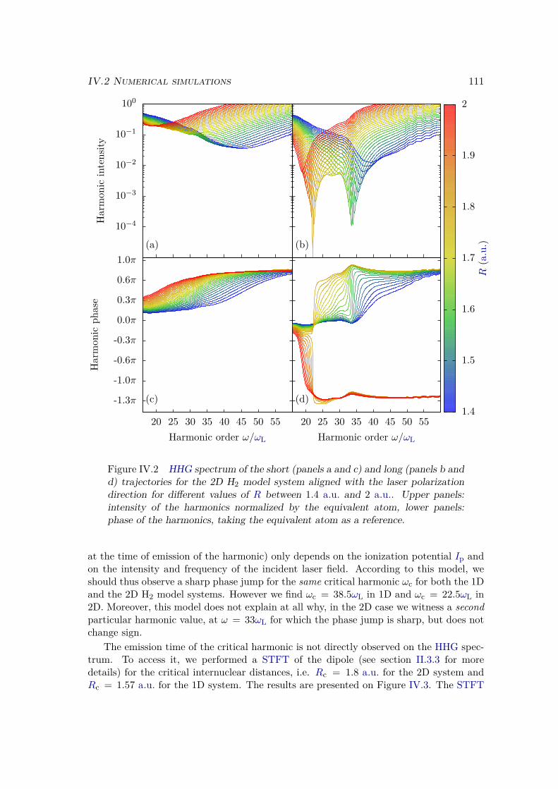
IV.2 Numerical simulations 111
10−4
10−3
10−2
10−1
100
(a) (b)
-1.3π
-1.0π
-0.6π
-0.3π
0.0π
0.3π
0.6π
1.0π
20 25 30 35 40 45 50 55
(c)
20 25 30 35 40 45 50 55
(d)
Harmon
icintensity
Harmon
icph
ase
Harmonic order ω/ωL Harmonic order ω/ωL
1.4
1.5
1.6
1.7
1.8
1.9
2
R(a.u.)
Figure IV.2 HHG spectrum of the short (panels a and c) and long (panels b andd) trajectories for the 2D H2 model system aligned with the laser polarizationdirection for different values of R between 1.4 a.u. and 2 a.u.. Upper panels:intensity of the harmonics normalized by the equivalent atom, lower panels:phase of the harmonics, taking the equivalent atom as a reference.
at the time of emission of the harmonic) only depends on the ionization potential Ip andon the intensity and frequency of the incident laser field. According to this model, weshould thus observe a sharp phase jump for the same critical harmonic ωc for both the 1Dand the 2D H2 model systems. However we find ωc = 38.5ωL in 1D and ωc = 22.5ωL in2D. Moreover, this model does not explain at all why, in the 2D case we witness a secondparticular harmonic value, at ω = 33ωL for which the phase jump is sharp, but does notchange sign.
The emission time of the critical harmonic is not directly observed on the HHG spec-trum. To access it, we performed a STFT of the dipole (see section II.3.3 for moredetails) for the critical internuclear distances, i.e. Rc = 1.8 a.u. for the 2D system andRc = 1.57 a.u. for the 1D system. The results are presented on Figure IV.3. The STFT
112 Chapter IV. Two-center interferences in HHG
has the expected bell shape, which allows a direct mapping of two different emission timesfor each harmonic, corresponding to the emission times of the short and of the long tra-jectories. In both cases we observe a dip in the spectrum, corresponding to the 2-centerinterference minimum. In agreement with our previous observations, we find that thisdip is located on the part that corresponds to the long trajectories, and that it appearsat a harmonic of ωc = 22.5ωL for the 2D system (panel (a)) and ωc = 38.5ωL for the 1Dsystem (panel (b)). It becomes clear on this figure that the emission time of this criticalharmonic are very different in the 2D and in the 1D case: we find tc = 1.63 TL in 2Dand tc = 1.47 TL in 1D. Moreover, in both cases, this coincides with a non zero electricfield at the time of emission of the harmonic.
These findings are thus in disagreement with the interpretation that the smoothing ofthe phase jump would simply be a consequence of the dressing of the ground state by theelectric field. It is also in disagreement with the conclusion of François Risoud in [129].However we saw in section IV.1.3 that in the calculation performed by François Risoud,the influence of the saddle point prefactor was neglected. We shown in section IV.1 that,by adding this contribution, the phase jump was not necessarily sharp for a zero electricfield at the recombination time. Instead we found a different condition, given in (IV.43),which, in the LCAO approximation, explicitly depends on the orbital Fourrier transformand on its derivative. Our calculation thus allows to understand why the shape of theminimum and phase jump may actually depend on the system geometry, and not only onits ionization potential as was suggested in [129]. These disparities between the 1D andthe 2D simulations may also be caused by the difference of spreading of the wave packetduring the propagation step. Indeed, in 2D the ionized wave packet has the possibility tospread in the direction transverse to the propagation, which is forbidden in 1D.
To better understand the differences between the 1D and the 2D case, we performedthe same analysis on the intermediate system presented in the previous section. Forthese systems, the electron is trapped in a stretched two dimensional potential. Theground state is thus closer to the 1D case, but the electron wave packet still has thepossibility to spread in two dimensions, which is impossible in 1D. This is why we callthem "intermediate" between 1D and 2D.
The results are presented on Figure IV.4 for a system with κ = 0.1 a.u. and onFigure IV.5 for a system with κ = 0.5 a.u.. The spectrum intensity and phase arecomparable to the previous results. For a given value of R, the harmonic where theminimum appears (and the phase jump) is always the same, with only small differences,for all the systems that we considered in this section. Here again the shape of the minimumand of the phase jump that we observe in the short trajectories is very similar to theprevious observations: it is always smoothed and cover several harmonics. The spectrumof the long trajectories behaves differently. Interestingly we find that, for the system thatis the most stretched i.e. with κ = 0.1, the minimum and the phase jump appear verysharp for the same critical harmonic ωc = 38.5ωL as in the 1D case. By performingthe STFT of the dipole we also find that it corresponds to the same emission time oftc = 1.47 TL. As we said, an electron trapped in this 2D stretched potential behavessimilarly to a 1D electron, except that the ionized wave packet has the possibility tospread in the transverse direction during the propagation in the continuum. Therefore,the fact that the 1D and the stretched 2D potentials have the same critical harmonicseems to indicate that this spreading of the wave packet does play a role in the 2-center
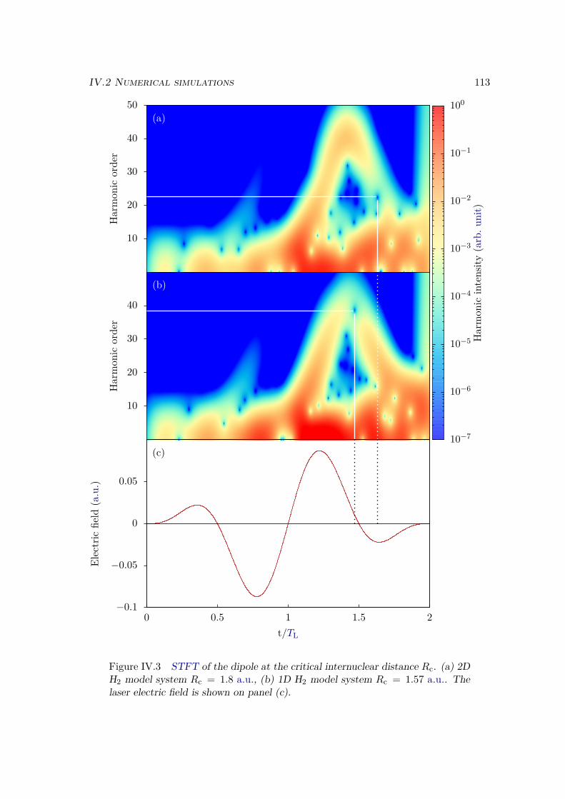
IV.2 Numerical simulations 113
10
20
30
40
50
10
20
30
40
−0.1
−0.05
0
0.05
0 0.5 1 1.5 2
Harmon
icorde
r(a)
Harmon
icorde
r
10−7
10−6
10−5
10−4
10−3
10−2
10−1
100
Harmon
icintensity
(arb.
unit)
(b)
Electric
field
(a.u.)
t/TL
(c)
Figure IV.3 STFT of the dipole at the critical internuclear distance Rc. (a) 2DH2 model system Rc = 1.8 a.u., (b) 1D H2 model system Rc = 1.57 a.u.. Thelaser electric field is shown on panel (c).
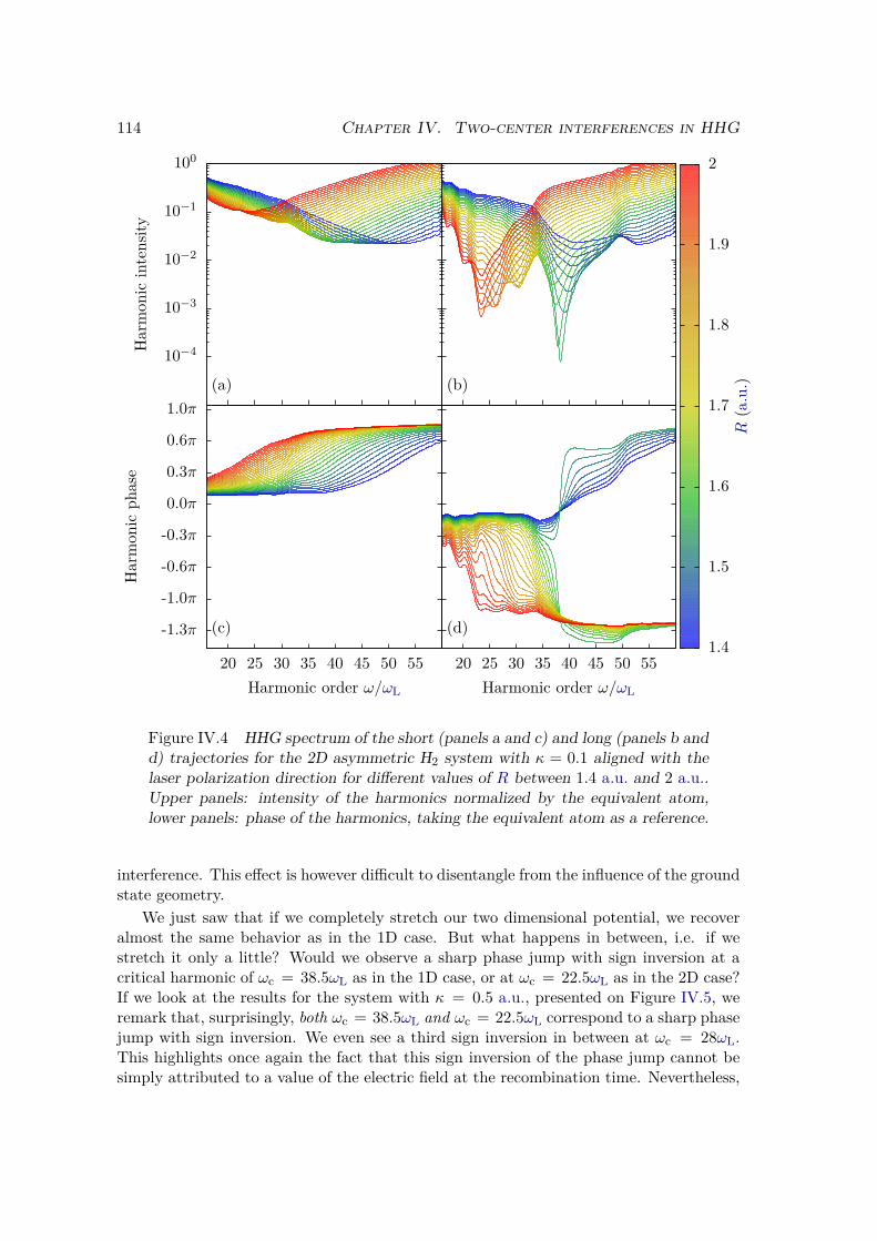
114 Chapter IV. Two-center interferences in HHG
10−4
10−3
10−2
10−1
100
(a) (b)
-1.3π
-1.0π
-0.6π
-0.3π
0.0π
0.3π
0.6π
1.0π
20 25 30 35 40 45 50 55
(c)
20 25 30 35 40 45 50 55
(d)
Harmon
icintensity
Harmon
icph
ase
Harmonic order ω/ωL Harmonic order ω/ωL
1.4
1.5
1.6
1.7
1.8
1.9
2
R(a.u.)
Figure IV.4 HHG spectrum of the short (panels a and c) and long (panels b andd) trajectories for the 2D asymmetric H2 system with κ = 0.1 aligned with thelaser polarization direction for different values of R between 1.4 a.u. and 2 a.u..Upper panels: intensity of the harmonics normalized by the equivalent atom,lower panels: phase of the harmonics, taking the equivalent atom as a reference.
interference. This effect is however difficult to disentangle from the influence of the groundstate geometry.
We just saw that if we completely stretch our two dimensional potential, we recoveralmost the same behavior as in the 1D case. But what happens in between, i.e. if westretch it only a little? Would we observe a sharp phase jump with sign inversion at acritical harmonic of ωc = 38.5ωL as in the 1D case, or at ωc = 22.5ωL as in the 2D case?If we look at the results for the system with κ = 0.5 a.u., presented on Figure IV.5, weremark that, surprisingly, both ωc = 38.5ωL and ωc = 22.5ωL correspond to a sharp phasejump with sign inversion. We even see a third sign inversion in between at ωc = 28ωL.This highlights once again the fact that this sign inversion of the phase jump cannot besimply attributed to a value of the electric field at the recombination time. Nevertheless,
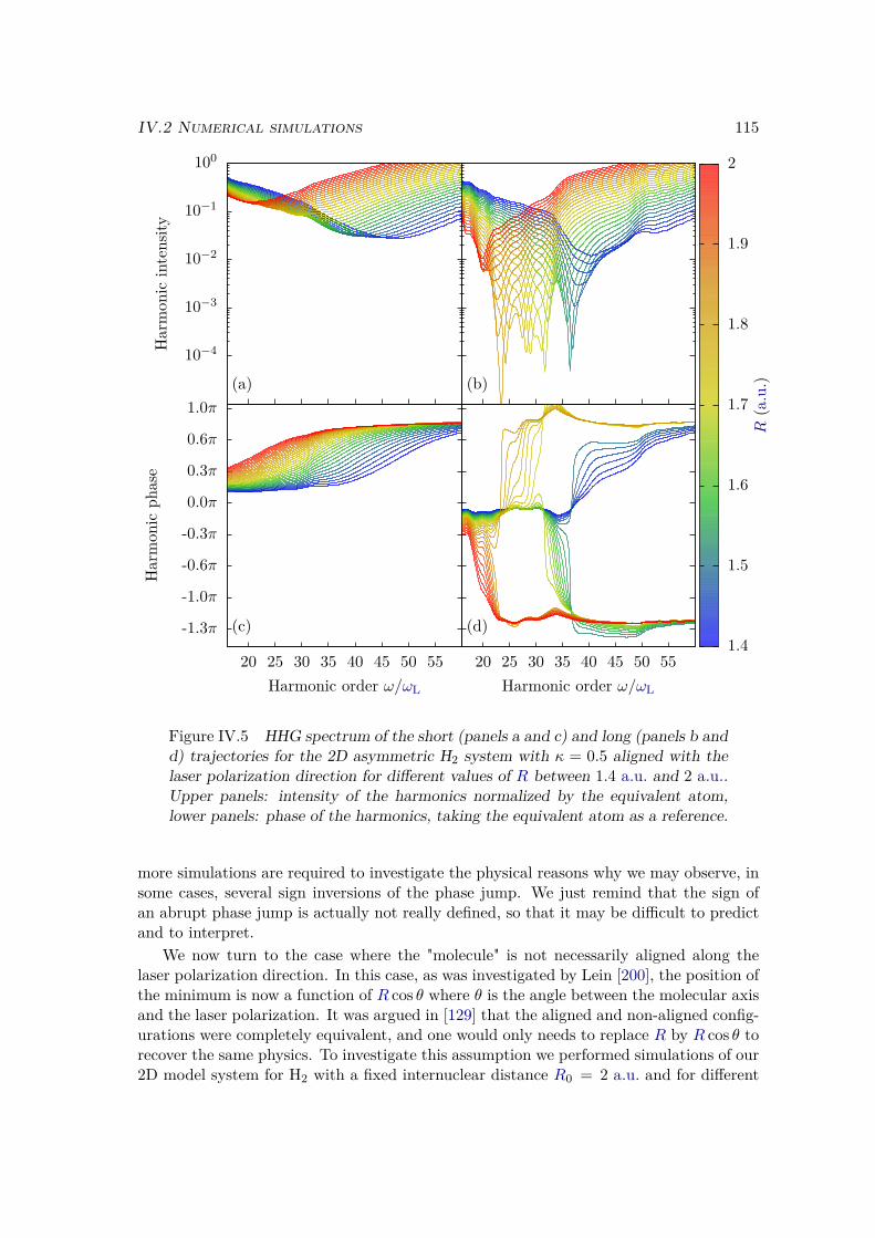
IV.2 Numerical simulations 115
10−4
10−3
10−2
10−1
100
(a) (b)
-1.3π
-1.0π
-0.6π
-0.3π
0.0π
0.3π
0.6π
1.0π
20 25 30 35 40 45 50 55
(c)
20 25 30 35 40 45 50 55
(d)
Harmon
icintensity
Harmon
icph
ase
Harmonic order ω/ωL Harmonic order ω/ωL
1.4
1.5
1.6
1.7
1.8
1.9
2
R(a.u.)
Figure IV.5 HHG spectrum of the short (panels a and c) and long (panels b andd) trajectories for the 2D asymmetric H2 system with κ = 0.5 aligned with thelaser polarization direction for different values of R between 1.4 a.u. and 2 a.u..Upper panels: intensity of the harmonics normalized by the equivalent atom,lower panels: phase of the harmonics, taking the equivalent atom as a reference.
more simulations are required to investigate the physical reasons why we may observe, insome cases, several sign inversions of the phase jump. We just remind that the sign ofan abrupt phase jump is actually not really defined, so that it may be difficult to predictand to interpret.
We now turn to the case where the "molecule" is not necessarily aligned along thelaser polarization direction. In this case, as was investigated by Lein [200], the position ofthe minimum is now a function of R cos θ where θ is the angle between the molecular axisand the laser polarization. It was argued in [129] that the aligned and non-aligned config-urations were completely equivalent, and one would only needs to replace R by R cos θ torecover the same physics. To investigate this assumption we performed simulations of our2D model system for H2 with a fixed internuclear distance R0 = 2 a.u. and for different
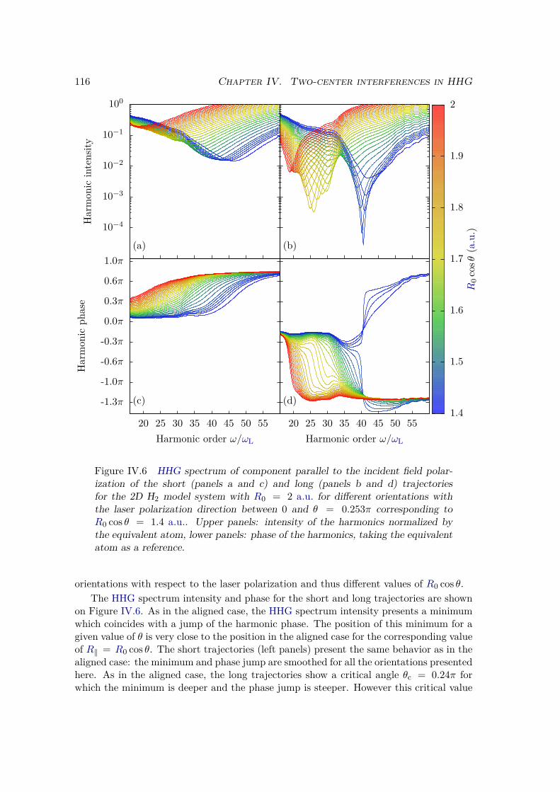
116 Chapter IV. Two-center interferences in HHG
10−4
10−3
10−2
10−1
100
(a) (b)
-1.3π
-1.0π
-0.6π
-0.3π
0.0π
0.3π
0.6π
1.0π
20 25 30 35 40 45 50 55
(c)
20 25 30 35 40 45 50 55
(d)
Harmon
icintensity
Harmon
icph
ase
Harmonic order ω/ωL Harmonic order ω/ωL
1.4
1.5
1.6
1.7
1.8
1.9
2
R0
cosθ
(a.u.)
Figure IV.6 HHG spectrum of component parallel to the incident field polar-ization of the short (panels a and c) and long (panels b and d) trajectoriesfor the 2D H2 model system with R0 = 2 a.u. for different orientations withthe laser polarization direction between 0 and θ = 0.253π corresponding toR0 cos θ = 1.4 a.u.. Upper panels: intensity of the harmonics normalized bythe equivalent atom, lower panels: phase of the harmonics, taking the equivalentatom as a reference.
orientations with respect to the laser polarization and thus different values of R0 cos θ.The HHG spectrum intensity and phase for the short and long trajectories are shown
on Figure IV.6. As in the aligned case, the HHG spectrum intensity presents a minimumwhich coincides with a jump of the harmonic phase. The position of this minimum for agiven value of θ is very close to the position in the aligned case for the corresponding valueof R‖ = R0 cos θ. The short trajectories (left panels) present the same behavior as in thealigned case: the minimum and phase jump are smoothed for all the orientations presentedhere. As in the aligned case, the long trajectories show a critical angle θc = 0.24π forwhich the minimum is deeper and the phase jump is steeper. However this critical value
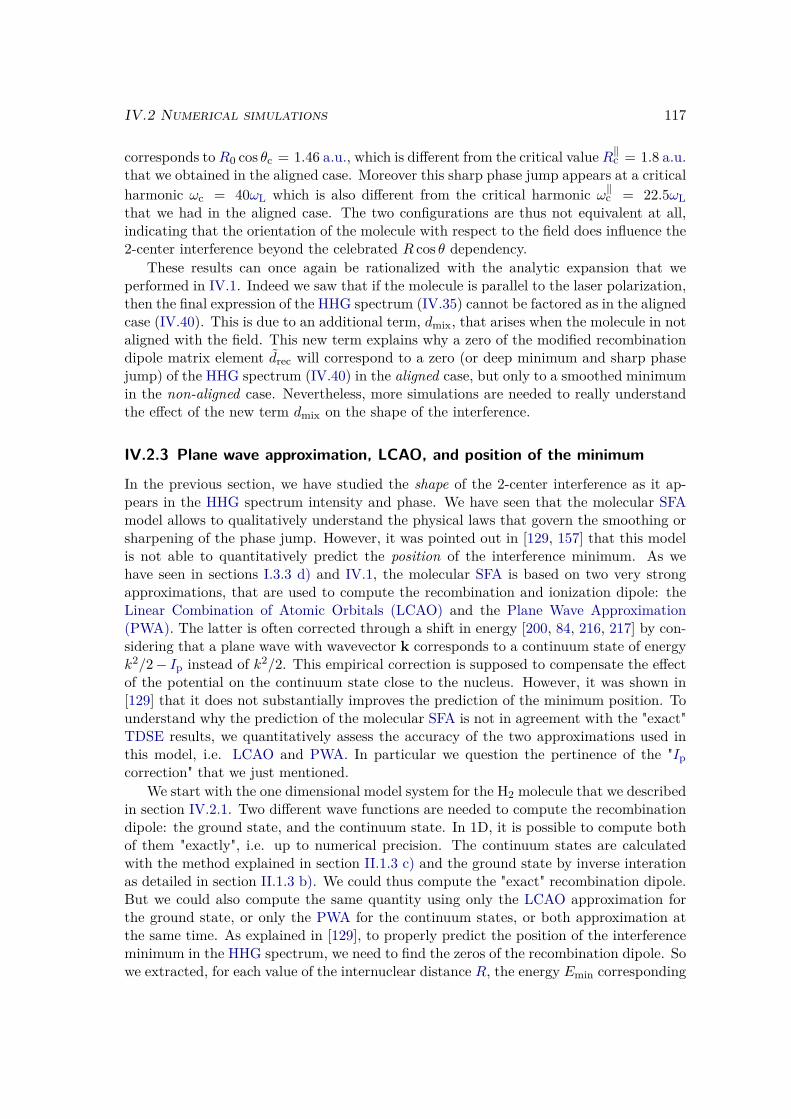
IV.2 Numerical simulations 117
corresponds toR0 cos θc = 1.46 a.u., which is different from the critical valueR‖c = 1.8 a.u.that we obtained in the aligned case. Moreover this sharp phase jump appears at a criticalharmonic ωc = 40ωL which is also different from the critical harmonic ω‖c = 22.5ωLthat we had in the aligned case. The two configurations are thus not equivalent at all,indicating that the orientation of the molecule with respect to the field does influence the2-center interference beyond the celebrated R cos θ dependency.
These results can once again be rationalized with the analytic expansion that weperformed in IV.1. Indeed we saw that if the molecule is parallel to the laser polarization,then the final expression of the HHG spectrum (IV.35) cannot be factored as in the alignedcase (IV.40). This is due to an additional term, dmix, that arises when the molecule in notaligned with the field. This new term explains why a zero of the modified recombinationdipole matrix element drec will correspond to a zero (or deep minimum and sharp phasejump) of the HHG spectrum (IV.40) in the aligned case, but only to a smoothed minimumin the non-aligned case. Nevertheless, more simulations are needed to really understandthe effect of the new term dmix on the shape of the interference.
IV.2.3 Plane wave approximation, LCAO, and position of the minimum
In the previous section, we have studied the shape of the 2-center interference as it ap-pears in the HHG spectrum intensity and phase. We have seen that the molecular SFAmodel allows to qualitatively understand the physical laws that govern the smoothing orsharpening of the phase jump. However, it was pointed out in [129, 157] that this modelis not able to quantitatively predict the position of the interference minimum. As wehave seen in sections I.3.3 d) and IV.1, the molecular SFA is based on two very strongapproximations, that are used to compute the recombination and ionization dipole: theLinear Combination of Atomic Orbitals (LCAO) and the Plane Wave Approximation(PWA). The latter is often corrected through a shift in energy [200, 84, 216, 217] by con-sidering that a plane wave with wavevector k corresponds to a continuum state of energyk2/2− Ip instead of k2/2. This empirical correction is supposed to compensate the effectof the potential on the continuum state close to the nucleus. However, it was shown in[129] that it does not substantially improves the prediction of the minimum position. Tounderstand why the prediction of the molecular SFA is not in agreement with the "exact"TDSE results, we quantitatively assess the accuracy of the two approximations used inthis model, i.e. LCAO and PWA. In particular we question the pertinence of the "Ipcorrection" that we just mentioned.
We start with the one dimensional model system for the H2 molecule that we describedin section IV.2.1. Two different wave functions are needed to compute the recombinationdipole: the ground state, and the continuum state. In 1D, it is possible to compute bothof them "exactly", i.e. up to numerical precision. The continuum states are calculatedwith the method explained in section II.1.3 c) and the ground state by inverse interationas detailed in section II.1.3 b). We could thus compute the "exact" recombination dipole.But we could also compute the same quantity using only the LCAO approximation forthe ground state, or only the PWA for the continuum states, or both approximation atthe same time. As explained in [129], to properly predict the position of the interferenceminimum in the HHG spectrum, we need to find the zeros of the recombination dipole. Sowe extracted, for each value of the internuclear distance R, the energy Emin corresponding
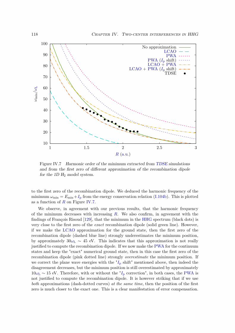
118 Chapter IV. Two-center interferences in HHG
10
20
30
40
50
60
70
80
90
100
1 1.5 2 2.5 3
ωm
in/ω
L
R (a.u.)
No approximationLCAOPWA
PWA (Ip shift)LCAO + PWA
LCAO + PWA (Ip shift)TDSE
Figure IV.7 Harmonic order of the minimum extracted from TDSE simulationsand from the first zero of different approximation of the recombination dipolefor the 1D H2 model system.
to the first zero of the recombination dipole. We deduced the harmonic frequency of theminimum ωmin = Emin +Ip from the energy conservation relation (I.104b). This is plottedas a function of R on Figure IV.7.
We observe, in agreement with our previous results, that the harmonic frequencyof the minimum decreases with increasing R. We also confirm, in agreement with thefindings of François Risoud [129], that the minimum in the HHG spectrum (black dots) isvery close to the first zero of the exact recombination dipole (solid green line). However,if we make the LCAO approximation for the ground state, then the first zero of therecombination dipole (dashed blue line) strongly underestimates the minimum position,by approximately 30ωL ∼ 45 eV. This indicates that this approximation is not reallyjustified to compute the recombination dipole. If we now make the PWA for the continuumstates and keep the "exact" numerical ground state, then in this case the first zero of therecombination dipole (pink dotted line) strongly overestimate the minimum position. Ifwe correct the plane wave energies with the "Ip shift" mentioned above, then indeed thedisagreement decreases, but the minimum position is still overestimated by approximately10ωL ∼ 15 eV. Therefore, with or without the "Ip correction", in both cases, the PWA isnot justified to compute the recombination dipole. It is however striking that if we useboth approximations (dash-dotted curves) at the same time, then the position of the firstzero is much closer to the exact one. This is a clear manifestation of error compensation.
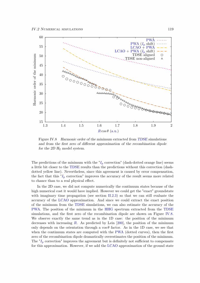
IV.2 Numerical simulations 119
15
20
25
30
35
40
45
50
55
60
1.3 1.4 1.5 1.6 1.7 1.8 1.9 2
Harmon
icorde
rof
theminim
um
R cos θ (a.u.)
PWAPWA (Ip shift)LCAO + PWA
LCAO + PWA (Ip shift)TDSE aligned
TDSE non-aligned
Figure IV.8 Harmonic order of the minimum extracted from TDSE simulationsand from the first zero of different approximation of the recombination dipolefor the 2D H2 model system.
The predictions of the minimum with the "Ip correction" (dash-dotted orange line) seemsa little bit closer to the TDSE results than the predictions without this correction (dash-dotted yellow line). Nevertheless, since this agreement is caused by error compensation,the fact that this "Ip correction" improves the accuracy of the result seems more relatedto chance than to a real physical effect.
In the 2D case, we did not compute numerically the continuum states because of thehigh numerical cost it would have implied. However we could get the "exact" groundstatewith imaginary time propagation (see section II.2.3) so that we can still evaluate theaccuracy of the LCAO approximation. And since we could extract the exact positionof the minimum from the TDSE simulations, we can also estimate the accuracy of thePWA. The position of the minimum in the HHG spectrum extracted from the TDSEsimulations, and the first zero of the recombination dipole are shown on Figure IV.8.We observe exactly the same trend as in the 1D case: the position of the minimumdecreases with increasing R. As predicted by Lein [200], the position of the minimumonly depends on the orientation through a cos θ factor. As in the 1D case, we see thatwhen the continuum states are computed with the PWA (dotted curves), then the firstzero of the recombination dipole dramatically overestimates the position of the minimum.The "Ip correction" improves the agreement but is definitely not sufficient to compensatefor this approximation. However, if we add the LCAO approximation of the ground state
120 Chapter IV. Two-center interferences in HHG
(dashed-dotted curves), then once again we compensate almost all the error that wasintroduced by the PWA.
One has thus to be extremely careful when trying to use the molecular SFA model tomake quantitative predictions. Indeed, the error compensation that we witness for theposition of the minimum is not guaranteed to be as efficient for other observables. Theremay very well be some cases where the errors of the two approximation add up insteadof compensating each other, with dramatic consequences.
IV.3 ConclusionIn this chapter we studied analytically and numerically the two center interference signa-ture that is observed in the HHG spectrum of diatomic molecules. We have completedthe analytical work of François Risoud in [129]. Our contribution allows to reach a betteragreement between the qualitative predictions of both approaches. In particular we couldexplain why the sharp interference structures in the spectrum were not observed for a zeroelectric field at recombination time. We found another condition for this sharpening, andwe saw that it strongly depends on the emitting system, and on the molecular orientationwith respect to the laser polarization. Our preliminary results seems to indicate that it isaffected by the spreading of the ionized wave packet during the propagation step as wellas the ground state geometry.
Finally we investigated the question of the quantitative agreement between the TDSEresults and the molecular SFA model developped by Chirilă and Lein [84]. We closelylooked at the effect of the LCAO and PWA on the computation of the recombinationdipole, and more precisely on the position of its first zero. We showed that each of thesetwo approximations induces a relatively large error of a few tens of eV on the predictionof the minimum position. However these errors almost perfectly compensate when weuse both approximations at the same time. This indicates that one must be very carefulwhen using the molecular SFA for quantitative predictions. Moreover this reduces theperspective of improvement of the model. Indeed any correction of the error induced byone of its underlying approximation may actually spoil this error compensation and wouldthus only deteriorate the accuracy. We believe that the main strength of the molecularSFA lies in its qualitative predictions, and on the physical interpretations that they bring,rather than on its quantitative accuracy.
Chapter V
Diatomic molecules in strong fields:ultrafast vibronic dynamics
In the previous chapters we studied the electronic dynamics of molecules submitted tostrong fields. We completely neglected the motion of the nuclei, and its influence on theelectrons. This approximation is justified if the nuclei can be considered to be very slowat the time scale of the electron dynamics. For heavy molecules the vibrational period istypically of the order of 100 fs, and the Titane:Sapphire laser has a period of 2.7 fs, sothat as long as the incident laser pulse is limited to a few optical cycles, we can considerthat the nuclei did not have sufficient time to move during the pulse. On the contrary,in the case of H2 the vibrational period in the ground state is 8 fs, we can thus start toobserve vibrational dynamics even during very short pulses of a few femtoseconds, see[220, 221] and references therein.
Recently, these femtosecond nuclear dynamics have been experimentally measured inD2 [222], where a fs infrared pulse induced a coherent transfer of population from theground to the first vibrational excited state of the Electronic Ground State (EGS). How-ever this population transfer raises the question of the vibrational excitation mechanism.Indeed for homonuclear diatomic molecules, the electric field does not couple the vibra-tional states within a given electronic state. The absorption of one or several photons isthus forbidden by symmetry. Two different mechanisms were proposed to explain this vi-brational excitation in the EGS: Bond-Softening (BS) and Lochfraß (LF) [223]. Both arebased on an adiabatic approach in a Born-Oppenheimer (BO) representation of the time-dependent wave function (V.10) where the electronic and nuclear dynamics are treatedseparately (see section V.1.2). The former, BS, is caused by the instantaneous Stark shiftES while the latter, LF, is caused by the instantaneous tunnel ionization rate Γ (II.70).In the Born-Oppenheimer representation (V.15) they can be seen as potential terms thatdepend on the internuclear distance R, and that effectively distort the Potential EnergySurface (PES) of the electronic ground state. The Stark shift distorts the real part of thePES while the ionization rate distorts its imaginary part, i.e. the lifetime of the dressedstate [224, 225]. Both effects thus occur simultaneously, and may even interfere with eachother. Nevertheless they behave differently and were given different interpretations [223].
In the case of the BS, since the polarizability of the molecule increases with theinternuclear distance, the Stark shift attracts the Nuclear Wave Packet (NWP) towards
121
122 Chapter V. Vibronic dynamics in strong fields
larger values of R, and induces some nuclear dynamics. In this mechanism it is thecoupling of the electronic ground state to the excited states, and especially to the firstexcited states, that causes the Stark shift, and hence the nuclear dynamics. It is generallyaccepted that another interpetation of the BS can be given in terms of Raman two-photontransitions [222], where both photon energies are found within the broad frequency widthof the femtosecond pulse. The adiabatic interpretation relies on the states that are dressedby the instantaneous electric field, while the Raman interpretation relies on field-freestates.
The other mechanism, LF (which can be translated from german as whole eating), iscaused by the instantaneous tunnel ionization rate. In general the R-dependence of theionization rate will be mostly inherited from the R-dependence of the vertical ionizationpotential defined within the BO framework as Ip(R) = EH+
2(R) − EH2(R). Indeed, as
we saw in Chapter III, the tunnel ionization rate depends exponentially on the ionizationpotential. For values of R that remain close to the equilibrium distance, the ionizationpotential decreases with R, and the ionization rate thus increases with R. The acceptedinterpretation, initially given in [223, 222], is that the electronic ground state is depop-ulated ("eaten") faster at large internuclear distances, inducing a nuclear dynamics. Inthis mechanism the nuclear dynamics is caused by the coupling of the electronic groundstate to the continuum states.
Although the BS and LF mechanisms occur simultaneously and may in principleinterfere, they are usually thought of as being independent from each other, and are thustreated separately [222, 223, 226]. For BS one needs to solve the BO nuclear TDSE (V.15)taking into account only the Stark shift ES, while for LF one solves (V.15) with only theionization rate Γ. In the two cases one finds that, at the end of the pulse, some populationhas been transfered from the ground to the first vibrational excited state, and that thepopulation in the higher excited states remains negligible (see Figure V.3). The NWPthus starts to oscillate at a frequency ωvib equal to the energy difference between these twovibrational states (see Figure V.4). In particular the average value of R can be writtenas 〈R〉 = 〈R0〉+ δR cos(ωvibt− Φ), where the phase Φ of this oscillation depends on theconsidered mechanism. If one takes only LF into account then ΦLF = π, while if only BSis considered then ΦBS = π/2 [222]. This phase was experimentally measured in [222]for D2 where they obtained Φexp = 0.946π, and in [227] for I2 where Φexp = 0.81π. Inboth cases they concluded that it was a direct experimental proof of the observation ofLochfraß.
However there is no established theoretical background relating the value of this phaseΦ to the relative importance of LF and BS which would support such a conclusion. Be-sides, simulations that include only one or the other of the two mechanisms are somewhatartificial. To justify such a separation, one would have to consider that BS and LF arecompletely decoupled. This is far from being intuitive, since they can occur simultane-ously, and both affect the NWP dynamics. For example we might see some enhancementeffects since BS attracts the NWP towards larger values or R where LF is more efficient,or on the contrary some inhibition since LF localizes the NWP towards smaller valuesof R where BS is less efficient. Moreover, to the best of our knowledge, there have beenno rigorous derivation of the modified nuclear TDSE (V.15) that would prove that theelectronic degrees of freedom could be averaged in such a way. In particular, the effectsof the nuclei-electron correlation which is completely neglected in this model has never
V.1 Methods 123
been investigated.In this work we question the ability of the uncorrelated BO framework to describe
the vibronic dynamics of diatomic molecules in strong laser fields. We study a simple2D model system, with one dimension for the electron position x and one dimensionfor the internuclear distance R. We first assess the qualitative relevance of the previousapproaches [222, 223, 226] where the LF and BS mechanisms were treated separately. Wecompare the predictions of the LF and BS to the full BO model where both mechanismsare included to question the limits of the interpretations based on the LF/BS dichotomie.Then we investigate the limits of the this BO model by comparing its results to fullycorrelated bidimensional simulations. Finally, we propose a consistent analytic derivationof the nuclear TDSE for the case of BS, and we give hints for the derivation of the totalBO model that would also include LF.
Objectives
ü Derive analytically the nuclear TDSE in the Born-Oppenheimer and adiabatic ap-proximations.
ü Find the limits of this approach to describe nuclear dynamics in strong fields.
ü Investigate the effects of the correlation between the nuclei and the electrons.
V.1 Methods
We investigate the nuclear dynamics of a homonuclear diatomic model molecule submittedto a strong femtosecond infrared pulse. We use two different approaches: the Born-Oppenheimer adiabatic approach that was proposed in [223] taking into account both theBS and LF, and a correlated approach where both nuclear and electron are treated withinthe same level of theory. We use a 2D model system, where the electron is confined in thedirection of the molecular axis, for which extensive simulations can easily be performed.It can be argued that the BS mechanism is predominant on the LF in this case. Indeedthe Stark shift, which is responsible for BS but that inhibits tunnel ionization and thusLF, is maximal for a parallel alignment of the molecule with the field. To be able tocompare BS and LF, we thus consider different model systems: (i) an analogue of H2, (ii)a more artificial system (in the sense that it has no direct physical analogue), that we willcall A2 in the following, for which LF is enhanced, and (iii) to investigate the role of theelectronic excited states, we also consider and a short range system that we call G2 thathas only two bound electronic states.
V.1.1 Two dimensional model systems
We consider 2D model systems like the one described in section II.2.1 where the firstdimension corresponds to the electron position x, and the second dimension to the inter-nuclear distance R. The total Hamiltonian reads:
H(x,R, t) = − 12µ
∂2
∂R2 −12∂2
∂x2 + VNN(R) + VNe(x,R) +Hint(x, t) (V.1)
124 Chapter V. Vibronic dynamics in strong fields
where the first two terms are kinetic energy terms with µ the reduced mass of the nuclei,VNN is the nucleus-nucleus interaction which will be taken to be equal to the PES ofthe ground state of H+
2 , VNe is the nuclei-electron interaction potential and Hint is theinteraction with the field. To remain consistent with the adiabatic approximation whichis formulated in length gauge, we will use the expression:
Hint = xFL(t). (V.2)
The nucleus-electron interaction depends on the system. For the H2 analogue we use amolecular Soft-Coulomb potential:
V H2Ne (x,R) = − 0.5√
a(R)2 + (x+R/2)2− 0.5√
a(R)2 + (x−R/2)2, (V.3)
where the regularization parameter a(R) is adapted so that the electronic ground stateat each value of R has the same energy as the one of the real H2 molecule. Our systemis to some extent comparable to a real H2 molecule that would be aligned with the laserelectric field. In particular the BO vibrational states and energies are identical.
We also define the system A2 for which we use a simple Soft-Coulomb potential:
V A2Ne (x,R) = − 1√
a(R)2 + (x+R/2)2, (V.4)
where again we fit the regularization parameter a(R) so that the electronic ground stateenergy matches the one of the real H2 molecule. This system has no physical counterpart,but it will have a nuclear dynamics quite close to the one of H2 since it evolves on thesame PES. In particular since it is a single-well potential, its polarizability is stronglyreduced, so that LF is enhanced with respect to BS.
Finally, to study the influence of the electronic excited states, we also consider asystem, that we call G2. For this system we use a short range Gaussian potential:
V G2Ne (x,R) = −A(R) e−(x+R/2)2/2σ −A(R) e−(x−R/2)2/2σ, (V.5)
where again the prefactor A(R) is fitted so that the electronic ground state energy matchesthe one of the real H2 molecule and where we chose σ = 0.8 a.u. so that the system hasonly one electronic excited state.
The TDSE is solved with the split-operator method described in section II.2.2. Toavoid unphysical reflections at the borders of the simulation box, we use absorbing con-ditions (II.32) with a width of habs = 100 a.u. in the x dimension of the grid (seesection II.1.2 c)). The results obtained this way are exact up to numerical accuracy andwill be considered as a reference in the following. We will denote them as the XR re-sults. In this representation the wave function is computed on a bidimensional grid, sothat we get all possible excited and ionized states. To compare with the experiments[222, 227] that measure the average value of R in the Electronic Ground State (EGS)〈R〉EGS, we will project our 2D wave function on the EGS ϕ(BO)
0 (x;R) computed with theBO approximation
ψEGS(x,R, t) = ϕ(BO)0 (x;R)
∫ϕ
(BO)0 (x′;R)ψ(x′, R, t) dx′√∫ ∣∣∣∫ ϕ(BO)0 (x′;R)ψ(x′, R, t) dx′
∣∣∣2 dR. (V.6)
V.1 Methods 125
and compute the average value of R in this projected wave function |ψEGS(t)〉:
〈R〉EGS (t) = 〈ΨEGS(t)|R|ΨEGS(t)〉 (V.7)
=∫R∣∣∣∫ ϕ(BO)
0 (x;R)ψ(x,R, t) dx∣∣∣2 dR∫ ∣∣∣∫ ϕ(BO)
0 (x′;R)ψ(x′, R, t) dx′∣∣∣2 dR
. (V.8)
From the wave function we also have a direct access to the population Pi(t) in the exactvibronic states of the molecule ϕi(x,R), by simple projection:
Pi(t) =∣∣∣∣∫ ϕi(x,R)ψ(x,R, t) dx dR
∣∣∣∣2 . (V.9)
V.1.2 Born Oppenheimer and adiabatic approximationsIn the same spirit as the usual time-independent BO formalism, the wave function isfactored in an electronic and a nuclear contribution:
ψ(x,R, t) = ϕ0(x;R, t)χ(R, t), (V.10)
where ϕ0(x;R, t) is the electronic ground state dressed by the instantaneous electricfield FL(t) for which R and t are just parameters, and χ(R, t) is the nuclear wave packetthat propagates on this dressed electronic state. The adiabatic approximation supposesthat this field-dressed state ϕ0(x;R, t) instantaneously adapt to the value of the time-dependent electric field. It is thus solution, for each time t, of the field-dressed electronictime-"independent" (in the sense that the time is just a constant parameter) Schrödingerequation:[
−12∂2
∂x2 + VNe(x,R) + xFL(t)]ϕ0(x;R, t) = ε0
(R,FL(t)
)ϕ0(x;R, t), (V.11)
where Hel(x,R, t) = −12∂2
∂x2 +VNe(x,R)+xFL(t) is the electronic Hamiltonian comprisingthe kinetic energy of the electrons −1
2∂2
∂x2 , the electron-nuclei interaction potential VNe,and the electron-field interaction in length gauge xFL(t) (see section I.1.2), and where thefield-dressed energy is given by
ε0(R,F ) = E0(R) + ES(R,F )− iΓ(R,F )2 , (V.12)
where E0(R) is the field-free PES of the electronic ground state, ES is the DC Stark shift(see section II.1.4) and Γ is the tunnel ionization rate (see section II.3.1). It is importantto understand that in this representation, the internuclear distance R and the time t thatappear in (V.11) and (V.12) are only fixed parameters, and not variables. The fact that Ris a parameter is related to the BO approximation, while for t it is related to the adiabaticapproximation. The total TDSE (V.13) can thus be reorganized as (V.14):
i∂ψ∂t
(x,R, t) =[− 1
2µ∂2
∂R2 + VNN(R) +Hel
]ψ(x,R, t) (V.13)
iϕ0(x;R, t)∂χ∂t
(R, t) = ϕ0(x;R, t)[− 1
2µ∂2
∂R2 + VNN(R) + ε0(R,F )]χ(R, t). (V.14)
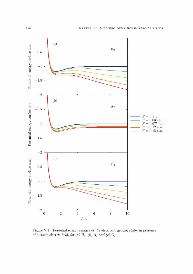
126 Chapter V. Vibronic dynamics in strong fields
−2
−1.5
−1
−0.5
(a)H2
−2
−1.5
−1
−0.5
(b)A2
−2
−1.5
−1
−0.5
0 2 4 6 8 10
(c)G2
Potentiale
nergysurfa
cea.
u.Po
tentiale
nergysurfa
cea.
u.
F = 0 a.u.F = 0.035 a.u.F = 0.075 a.u.F = 0.12 a.u.F = 0.15 a.u.
Potentiale
nergysurfa
cea.
u.
R a.u.
Figure V.1 Potential energy surface of the electronic ground state, in presenceof a static electric field, for (a) H2, (b) A2 and (c) G2.
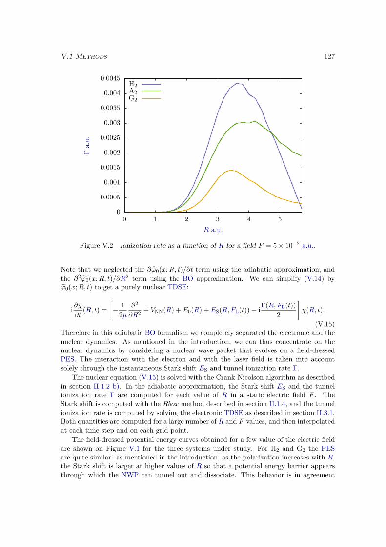
V.1 Methods 127
0
0.0005
0.001
0.0015
0.002
0.0025
0.003
0.0035
0.004
0.0045
0 1 2 3 4 5
Γa.
u.
R a.u.
H2A2G2
Figure V.2 Ionization rate as a function of R for a field F = 5× 10⁻² a.u..
Note that we neglected the ∂ϕ0(x;R, t)/∂t term using the adiabatic approximation, andthe ∂2ϕ0(x;R, t)/∂R2 term using the BO approximation. We can simplify (V.14) byϕ0(x;R, t) to get a purely nuclear TDSE:
i∂χ∂t
(R, t) =[− 1
2µ∂2
∂R2 + VNN(R) + E0(R) + ES(R,FL(t))− iΓ(R,FL(t))2
]χ(R, t).
(V.15)Therefore in this adiabatic BO formalism we completely separated the electronic and thenuclear dynamics. As mentioned in the introduction, we can thus concentrate on thenuclear dynamics by considering a nuclear wave packet that evolves on a field-dressedPES. The interaction with the electron and with the laser field is taken into accountsolely through the instantaneous Stark shift ES and tunnel ionization rate Γ.
The nuclear equation (V.15) is solved with the Crank-Nicolson algorithm as describedin section II.1.2 b). In the adiabatic approximation, the Stark shift ES and the tunnelionization rate Γ are computed for each value of R in a static electric field F . TheStark shift is computed with the Rbox method described in section II.1.4, and the tunnelionization rate is computed by solving the electronic TDSE as described in section II.3.1.Both quantities are computed for a large number of R and F values, and then interpolatedat each time step and on each grid point.
The field-dressed potential energy curves obtained for a few value of the electric fieldare shown on Figure V.1 for the three systems under study. For H2 and G2 the PESare quite similar: as mentioned in the introduction, as the polarization increases with R,the Stark shift is larger at higher values of R so that a potential energy barrier appearsthrough which the NWP can tunnel out and dissociate. This behavior is in agreement
128 Chapter V. Vibronic dynamics in strong fields
with the expected behavior in the real H2 molecule [224, 221]. The behavior of the PESis very different in the case of A2. Indeed, since there is only one potential well, thepolarizability is almost independent of R, and the PES are almost parallel. Since theStark shift does not strongly depend on R, it will almost not affect the nuclear dynamics,and the BS will be reduced and LF should dominate, which is exactly why we constructedthis system.
The ionization rates, computed by solving the TDSE in a static field F = 5×10⁻² a.u.for each model molecule, are shown in Figure V.2. We see that it behaves quite similarlyfor the three systems: it has a bell shape with a maximum located around 3.5 a.u., wellbeyond the equilibrium distance of R = 1.45 a.u.. This confirms that the ionizationrate has a positive slope near the equilibrium distance. Since ionization in this model isaccounted for by a R-dependent "absorption", LF should induce a motion of the NWPtowards small values of R.
V.2 ResultsThe three systems described in the previous section are submitted to various laser pulsesof central wavelength λL = 800 nm and of general shape:
FL(t) = F0 sin(ωLt+ φcep) sin2(ωL2Nc
t
), (V.16)
where ωL is the laser pulsation, Nc is the number of optical cycles in the pulse, and φcepis the Carrier Envelope Phase (CEP). We then follow the nuclear dynamics by computingthe populations in the different vibrational states and the average value of the internucleardistance. Note that in the BO approach, the average value of R is computed on the dressedEGS ϕ0(x;R) (V.11), while in correlated simulations we compute it on the field-free EGSϕ
(BO)0 (x;R). Nevertheless these two states become equivalent as soon as the laser pulse
is switched off, so that we will concentrate on the oscillations of the NWP after the endof the pulse.
We will first come back on the difference between Lochfraß and Bond-Softening, thenconfront the BO results, taking into account both LF and BS, to the correlated results,to be able to investigate the limits of the BO approach. Note that, to be consistent with[222, 223, 227], throughout this section we define the origin of time at the maximum ofthe laser pulse rather than at the beginning of the simulation. This allows to comparemore easily the results obtained with different pulse durations.
V.2.1 Lochfraß and Bond-SofteningWe start by comparing the differences and similarities between LF and BS. For thiswe solve the nuclear TDSE (V.15) including either the Stark shift ES or the ionizationrate Γ (V.12) or both (see section V.1.2). The population in the three first vibrationalexcited states during the pulse are shown in Figure V.3 for the H2 system submittedto an 8 optical cycle long pulse of intensity IL = 4 × 10¹⁴ W.cm−2. Note that inthe LF simulation, the population in the EGS decreases during the propagation due toionization. To compare with the BS case, we thus renormalize the population in thevibrational states to the total population in the EGS. We observe that, for both LF and
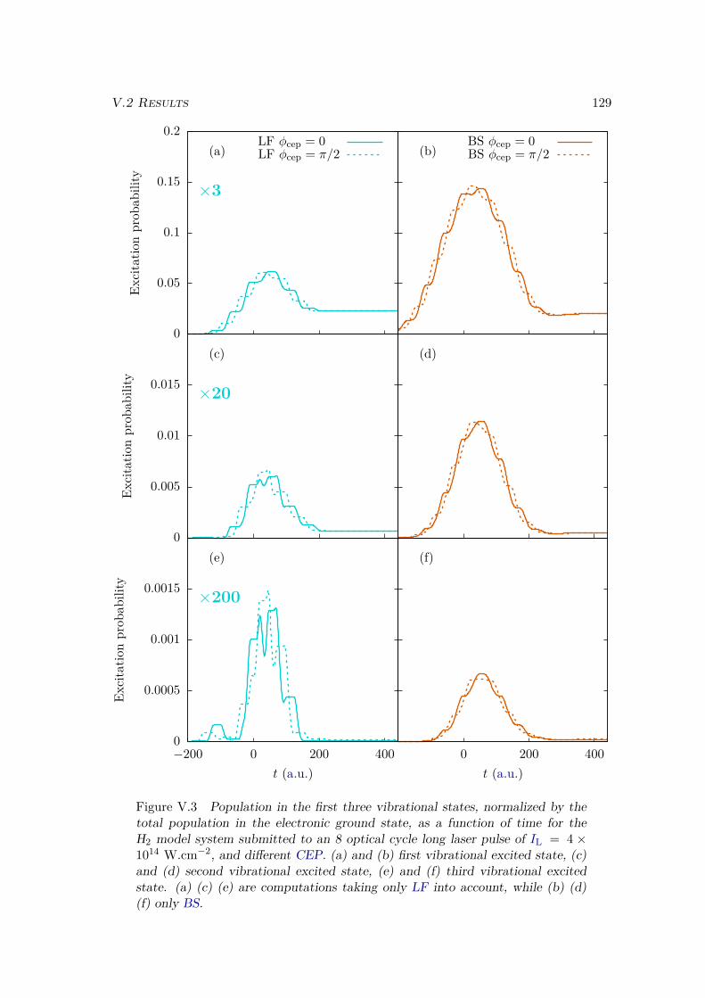
V.2 Results 129
0
0.05
0.1
0.15
0.2(a)
×3
(b)
0
0.005
0.01
0.015
(c)
×20
(d)
0
0.0005
0.001
0.0015
−200 0 200 400
(e)
×200
0 200 400
(f)
Excitatio
nprob
ability
LF φcep = 0LF φcep = π/2
BS φcep = 0BS φcep = π/2
Excitatio
nprob
ability
Excitatio
nprob
ability
t (a.u.) t (a.u.)
Figure V.3 Population in the first three vibrational states, normalized by thetotal population in the electronic ground state, as a function of time for theH2 model system submitted to an 8 optical cycle long laser pulse of IL = 4 ×10¹⁴ W.cm−2, and different CEP. (a) and (b) first vibrational excited state, (c)and (d) second vibrational excited state, (e) and (f) third vibrational excitedstate. (a) (c) (e) are computations taking only LF into account, while (b) (d)(f) only BS.
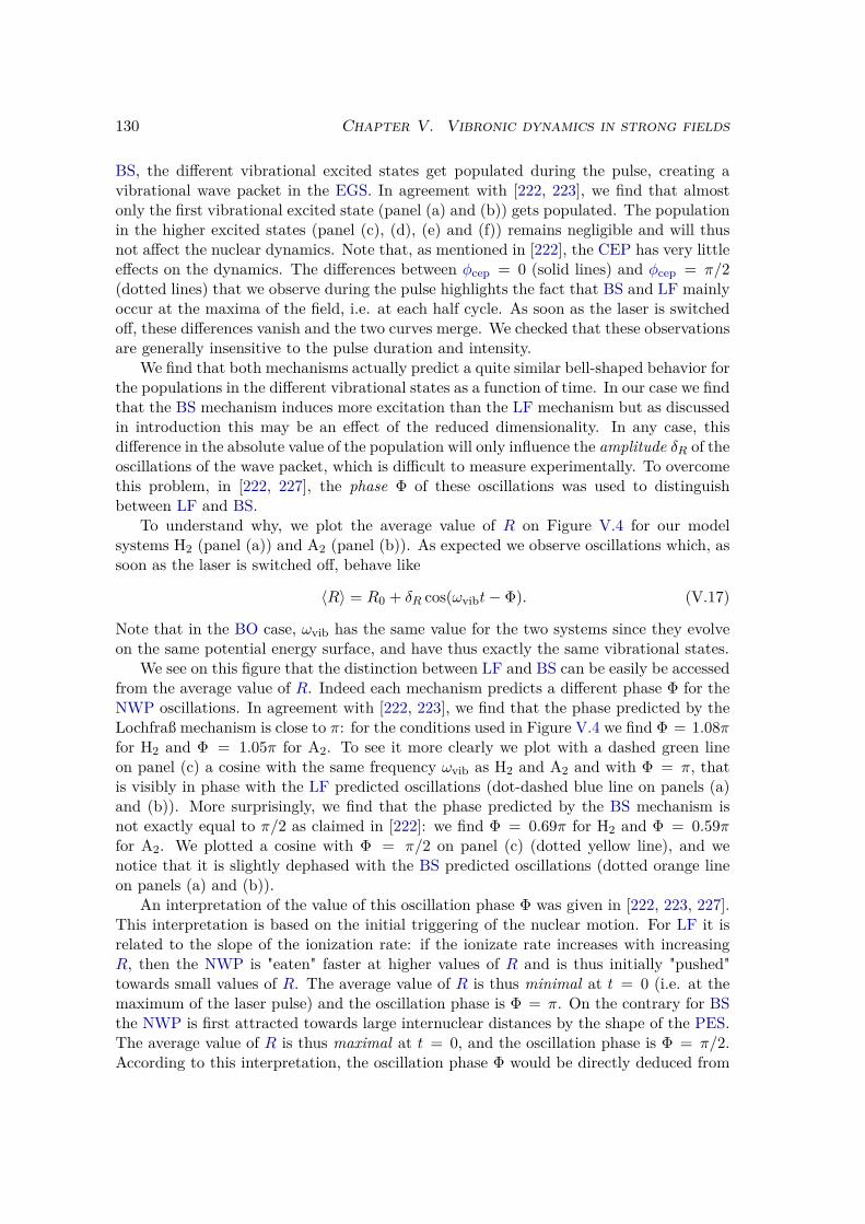
130 Chapter V. Vibronic dynamics in strong fields
BS, the different vibrational excited states get populated during the pulse, creating avibrational wave packet in the EGS. In agreement with [222, 223], we find that almostonly the first vibrational excited state (panel (a) and (b)) gets populated. The populationin the higher excited states (panel (c), (d), (e) and (f)) remains negligible and will thusnot affect the nuclear dynamics. Note that, as mentioned in [222], the CEP has very littleeffects on the dynamics. The differences between φcep = 0 (solid lines) and φcep = π/2(dotted lines) that we observe during the pulse highlights the fact that BS and LF mainlyoccur at the maxima of the field, i.e. at each half cycle. As soon as the laser is switchedoff, these differences vanish and the two curves merge. We checked that these observationsare generally insensitive to the pulse duration and intensity.
We find that both mechanisms actually predict a quite similar bell-shaped behavior forthe populations in the different vibrational states as a function of time. In our case we findthat the BS mechanism induces more excitation than the LF mechanism but as discussedin introduction this may be an effect of the reduced dimensionality. In any case, thisdifference in the absolute value of the population will only influence the amplitude δR of theoscillations of the wave packet, which is difficult to measure experimentally. To overcomethis problem, in [222, 227], the phase Φ of these oscillations was used to distinguishbetween LF and BS.
To understand why, we plot the average value of R on Figure V.4 for our modelsystems H2 (panel (a)) and A2 (panel (b)). As expected we observe oscillations which, assoon as the laser is switched off, behave like
〈R〉 = R0 + δR cos(ωvibt− Φ). (V.17)
Note that in the BO case, ωvib has the same value for the two systems since they evolveon the same potential energy surface, and have thus exactly the same vibrational states.
We see on this figure that the distinction between LF and BS can be easily be accessedfrom the average value of R. Indeed each mechanism predicts a different phase Φ for theNWP oscillations. In agreement with [222, 223], we find that the phase predicted by theLochfraß mechanism is close to π: for the conditions used in Figure V.4 we find Φ = 1.08πfor H2 and Φ = 1.05π for A2. To see it more clearly we plot with a dashed green lineon panel (c) a cosine with the same frequency ωvib as H2 and A2 and with Φ = π, thatis visibly in phase with the LF predicted oscillations (dot-dashed blue line on panels (a)and (b)). More surprisingly, we find that the phase predicted by the BS mechanism isnot exactly equal to π/2 as claimed in [222]: we find Φ = 0.69π for H2 and Φ = 0.59πfor A2. We plotted a cosine with Φ = π/2 on panel (c) (dotted yellow line), and wenotice that it is slightly dephased with the BS predicted oscillations (dotted orange lineon panels (a) and (b)).
An interpretation of the value of this oscillation phase Φ was given in [222, 223, 227].This interpretation is based on the initial triggering of the nuclear motion. For LF it isrelated to the slope of the ionization rate: if the ionizate rate increases with increasingR, then the NWP is "eaten" faster at higher values of R and is thus initially "pushed"towards small values of R. The average value of R is thus minimal at t = 0 (i.e. at themaximum of the laser pulse) and the oscillation phase is Φ = π. On the contrary for BSthe NWP is first attracted towards large internuclear distances by the shape of the PES.The average value of R is thus maximal at t = 0, and the oscillation phase is Φ = π/2.According to this interpretation, the oscillation phase Φ would be directly deduced from
V.2 Results 131
1.4
1.45
1.5
1.55
1.6(a) H2
1.42
1.44
1.46
1.48
1.5
1.52 (b) A2
−0.15
−0.1
−0.05
0
0.05
0.1
−1 0 1 2 3 4 5
(c)
〈R〉(a.u.)
BS + LFLFBS
〈R〉(a.u.)
Electric
field
(a.u.)
t/Tvib
Φ = πΦ = π/2
Figure V.4 Average value of the internuclear distance in the electronic groundstate for an 8 cycle long pulse of IL = 4×10¹⁴ W.cm−2, with a CEP of φcep = 0for (a) H2 and (b) A2. The laser field is drawn on panel (c), along with two cosinefunctions A cos(ωH2t− Φ) with arbitrary amplitude A. Gray lines are drawn attimes tn = nTvib
4 .
132 Chapter V. Vibronic dynamics in strong fields
the initial motion of the NWP: if it initially moves towards large R then Φ = π/2, whileif it initially moves towards small R then Φ = π
Yet this interpretation only holds as long as one considers BS and LF separately. Sincethey actually occur simultaneously, we need to include them both at the same time tocorrectly describe the dynamics. When we do so (dashed pink line on panels (a) and (b))we see that, for both systems, the average value of R is maximal at t = 0. The NWPthus starts to move towards large R, but the phase of the oscillation is close to Φ ' π.This is the opposite of the predictions given by the interpretation of [222, 223, 227] ! Thisindicates that there is actually no direct relation between the phase of the oscillationsand the displacement of the wave packet at t = 0. As a consequence, the slope ofthe ionization rate near the equilibrium distance cannot be deduced from this oscillationphase Φ, as was claimed in [227]. More importantly, it indicates that the interpretationof this oscillation phase is much more delicate than what was suggested in [222, 223, 227].
Since BS and LF predicts two very different values for the phase Φ of the NWPoscillations, it was claimed in [222, 223] that measuring the phase Φ could allow to dis-tinguish between the two mechanisms. This assumption is based on the hypothesis thatthe prevailing mechanism imposes its phase on the global oscillations. For example, inthe conditions used in Figure V.4, we see that, for the H2 systems, the BS mechanismpredicts a higher oscillation amplitude δR than LF and is thus the dominant mechanism.On the contrary, for A2 the oscillation amplitude δR predicted by LF is the highest, indi-cating that LF is prevailing. However if we look at the results predicted by the completemodel (dashed pink line), taking into account both LF and BS, we see that both H2 andA2, have the same phase for the wave packet oscillations. They both oscillate with a πphase, indicating that, in both cases, LF imposes its phase, even if it is not the dominantmechanism. This shows that the measure of Φ cannot allow to conclude on the prevailingmechanism, as was done in [222, 227].
To conclude, we find that the oscillation phase Φ is a consequence of the interplaybetween the two excitation mechanisms (LF and BS). It is thus very delicate to extractmeaningful information from this quantity.
V.2.2 Influence of the vibronic correlation
In the previous section we have seen that, in the BO framework, it is mandatory toconsider both LF and BS at the same time to get the proper behavior of the NWP. Ifone considers only one mechanism, this leads to unphysical results and interpretations.In this section, we investigate the limits of this BO model (with both LF and BS) byconfronting its predictions to fully correlated simulations that treats the active electronand the nuclei at the same level of theory.
First, we will clarify what we mean by the term "correlation". In general, the corre-lations are defined by "all that is not included in the uncorrelated model". In our case,it will thus include all that is not described by the BO representation of the wave func-tion. By looking at the two dimensional wave function, we see that the correlations mayoriginate from different contributions. These contributions are schetched on Figure V.5(a), where we draw them in the (x,R) plane. The contributions that are restricted tothe R axis (i) or to the x axis (ii) are uncorrelated. They do not couple x and R, sothat we expect them to be inlcuded in the BO model. On the other hand the diagonal
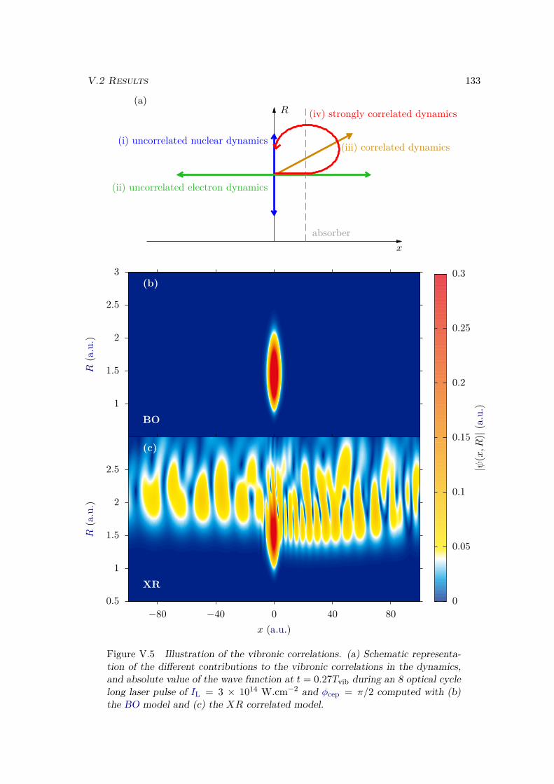
V.2 Results 133
1
1.5
2
2.5
3
0.5
1
1.5
2
2.5
−80 −40 0 40 80
(i) uncorrelated nuclear dynamics
(ii) uncorrelated electron dynamics
(iii) correlated dynamics
(iv) strongly correlated dynamics
absorber
R(a.u.)
(b)
BO
R(a.u.)
x (a.u.)
0
0.05
0.1
0.15
0.2
0.25
0.3
|ψ(x,R
)|(a.u.)
(c)
XR
x
R(a)
Figure V.5 Illustration of the vibronic correlations. (a) Schematic representa-tion of the different contributions to the vibronic correlations in the dynamics,and absolute value of the wave function at t = 0.27Tvib during an 8 optical cyclelong laser pulse of IL = 3 × 10¹⁴ W.cm−2 and φcep = π/2 computed with (b)the BO model and (c) the XR correlated model.
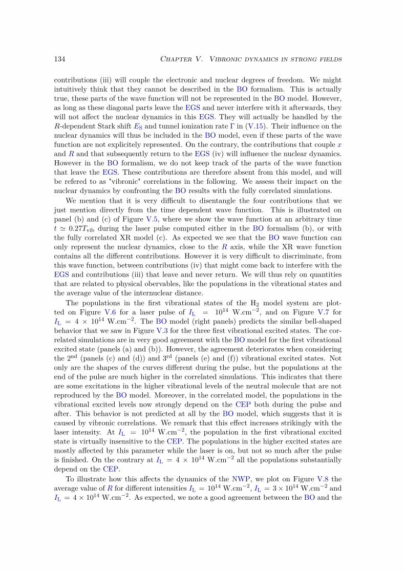
134 Chapter V. Vibronic dynamics in strong fields
contributions (iii) will couple the electronic and nuclear degrees of freedom. We mightintuitively think that they cannot be described in the BO formalism. This is actuallytrue, these parts of the wave function will not be represented in the BO model. However,as long as these diagonal parts leave the EGS and never interfere with it afterwards, theywill not affect the nuclear dynamics in this EGS. They will actually be handled by theR-dependent Stark shift ES and tunnel ionization rate Γ in (V.15). Their influence on thenuclear dynamics will thus be included in the BO model, even if these parts of the wavefunction are not explicitely represented. On the contrary, the contributions that couple xand R and that subsequently return to the EGS (iv) will influence the nuclear dynamics.However in the BO formalism, we do not keep track of the parts of the wave functionthat leave the EGS. These contributions are therefore absent from this model, and willbe refered to as "vibronic" correlations in the following. We assess their impact on thenuclear dynamics by confronting the BO results with the fully correlated simulations.
We mention that it is very difficult to disentangle the four contributions that wejust mention directly from the time dependent wave function. This is illustrated onpanel (b) and (c) of Figure V.5, where we show the wave function at an arbitrary timet ' 0.27Tvib during the laser pulse computed either in the BO formalism (b), or withthe fully correlated XR model (c). As expected we see that the BO wave function canonly represent the nuclear dynamics, close to the R axis, while the XR wave functioncontains all the different contributions. However it is very difficult to discriminate, fromthis wave function, between contributions (iv) that might come back to interfere with theEGS and contributions (iii) that leave and never return. We will thus rely on quantitiesthat are related to physical obervables, like the populations in the vibrational states andthe average value of the internuclear distance.
The populations in the first vibrational states of the H2 model system are plot-ted on Figure V.6 for a laser pulse of IL = 1014 W.cm−2, and on Figure V.7 forIL = 4 × 10¹⁴ W.cm−2. The BO model (right panels) predicts the similar bell-shapedbehavior that we saw in Figure V.3 for the three first vibrational excited states. The cor-related simulations are in very good agreement with the BO model for the first vibrationalexcited state (panels (a) and (b)). However, the agreement deteriorates when consideringthe 2nd (panels (c) and (d)) and 3rd (panels (e) and (f)) vibrational excited states. Notonly are the shapes of the curves different during the pulse, but the populations at theend of the pulse are much higher in the correlated simulations. This indicates that thereare some excitations in the higher vibrational levels of the neutral molecule that are notreproduced by the BO model. Moreover, in the correlated model, the populations in thevibrational excited levels now strongly depend on the CEP both during the pulse andafter. This behavior is not predicted at all by the BO model, which suggests that it iscaused by vibronic correlations. We remark that this effect increases strikingly with thelaser intensity. At IL = 1014 W.cm−2, the population in the first vibrational excitedstate is virtually insensitive to the CEP. The populations in the higher excited states aremostly affected by this parameter while the laser is on, but not so much after the pulseis finished. On the contrary at IL = 4 × 10¹⁴ W.cm−2 all the populations substantiallydepend on the CEP.
To illustrate how this affects the dynamics of the NWP, we plot on Figure V.8 theaverage value of R for different intensities IL = 1014 W.cm−2, IL = 3× 10¹⁴ W.cm−2 andIL = 4 × 10¹⁴ W.cm−2. As expected, we note a good agreement between the BO and the
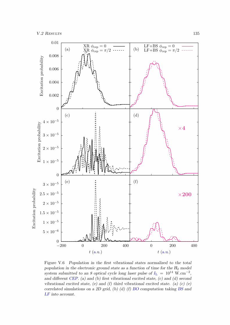
V.2 Results 135
0
0.002
0.004
0.006
0.008
0.01(a) (b)
0
1× 10⁻⁵
2× 10⁻⁵
3× 10⁻⁵
4× 10⁻⁵(c) (d)
×4
0
5× 10⁻⁶
1× 10⁻⁵
1.5× 10⁻⁵
2× 10⁻⁵
2.5× 10⁻⁵
3× 10⁻⁵
−200 0 200 400
(e)
0 200 400
(f)
×200
Excitatio
nprob
ability
XR φcep = 0XR φcep = π/2
LF+BS φcep = 0LF+BS φcep = π/2
Excitatio
nprob
ability
Excitatio
nprob
ability
t (a.u.) t (a.u.)
Figure V.6 Population in the first vibrational states normalized to the totalpopulation in the electronic ground state as a function of time for the H2 modelsystem submitted to an 8 optical cycle long laser pulse of IL = 1014 W.cm−2,and different CEP. (a) and (b) first vibrational excited state, (c) and (d) secondvibrational excited state, (e) and (f) third vibrational excited state. (a) (c) (e)correlated simulations on a 2D grid, (b) (d) (f) BO computation taking BS andLF into account.
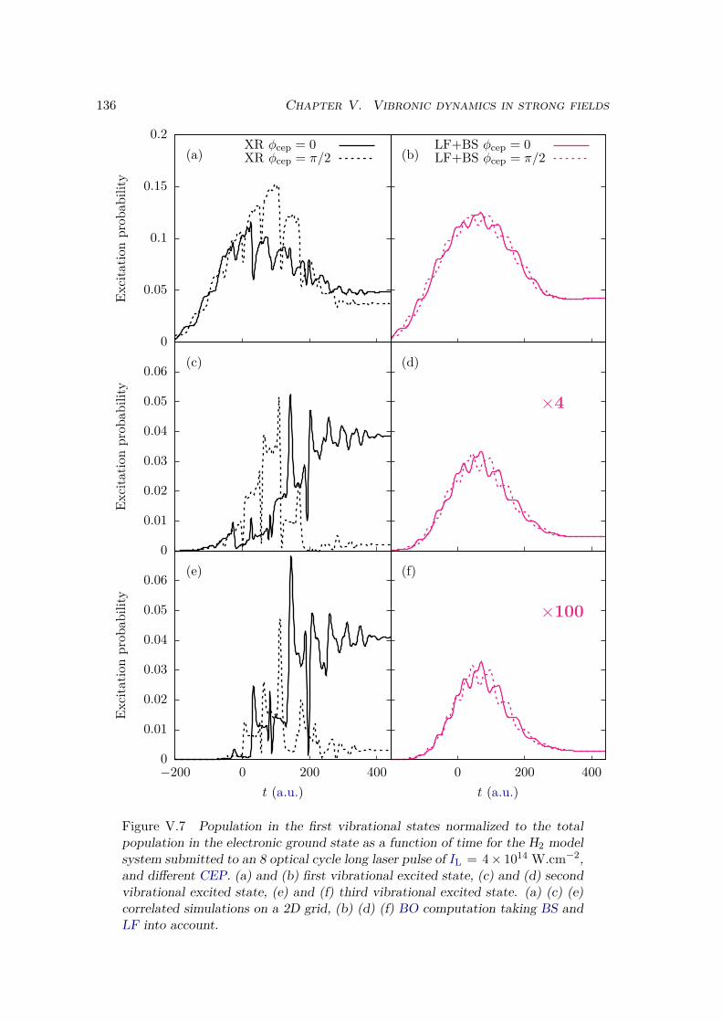
136 Chapter V. Vibronic dynamics in strong fields
0
0.05
0.1
0.15
0.2(a) (b)
0
0.01
0.02
0.03
0.04
0.05
0.06 (c) (d)
×4
0
0.01
0.02
0.03
0.04
0.05
0.06
−200 0 200 400
(e)
0 200 400
(f)
×100
Excitatio
nprob
ability
XR φcep = 0XR φcep = π/2
LF+BS φcep = 0LF+BS φcep = π/2
Excitatio
nprob
ability
Excitatio
nprob
ability
t (a.u.) t (a.u.)
Figure V.7 Population in the first vibrational states normalized to the totalpopulation in the electronic ground state as a function of time for the H2 modelsystem submitted to an 8 optical cycle long laser pulse of IL = 4× 10¹⁴ W.cm−2,and different CEP. (a) and (b) first vibrational excited state, (c) and (d) secondvibrational excited state, (e) and (f) third vibrational excited state. (a) (c) (e)correlated simulations on a 2D grid, (b) (d) (f) BO computation taking BS andLF into account.
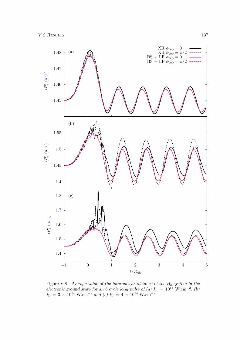
V.2 Results 137
1.45
1.46
1.47
1.48 (a)
1.4
1.45
1.5
1.55
(b)
1.4
1.5
1.6
1.7
1.8
−1 0 1 2 3 4 5
(c)
〈R〉(a.u.)
XR φcep = 0XR φcep = π/2
BS + LF φcep = 0BS + LF φcep = π/2
〈R〉(a.u.)
〈R〉(a.u.)
t/Tvib
Figure V.8 Average value of the internuclear distance of the H2 system in theelectronic ground state for an 8 cycle long pulse of (a) IL = 1014 W.cm−2, (b)IL = 3 × 10¹⁴ W.cm−2 and (c) IL = 4 × 10¹⁴ W.cm−2.
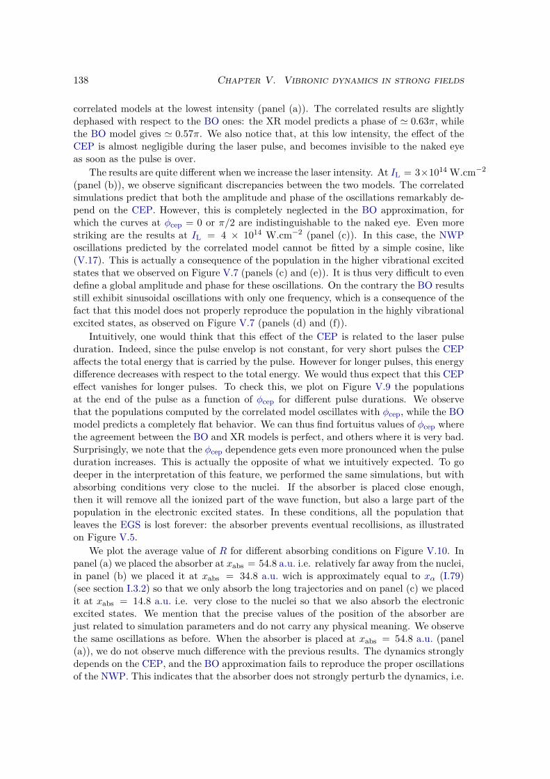
138 Chapter V. Vibronic dynamics in strong fields
correlated models at the lowest intensity (panel (a)). The correlated results are slightlydephased with respect to the BO ones: the XR model predicts a phase of ' 0.63π, whilethe BO model gives ' 0.57π. We also notice that, at this low intensity, the effect of theCEP is almost negligible during the laser pulse, and becomes invisible to the naked eyeas soon as the pulse is over.
The results are quite different when we increase the laser intensity. At IL = 3×10¹⁴ W.cm−2
(panel (b)), we observe significant discrepancies between the two models. The correlatedsimulations predict that both the amplitude and phase of the oscillations remarkably de-pend on the CEP. However, this is completely neglected in the BO approximation, forwhich the curves at φcep = 0 or π/2 are indistinguishable to the naked eye. Even morestriking are the results at IL = 4 × 10¹⁴ W.cm−2 (panel (c)). In this case, the NWPoscillations predicted by the correlated model cannot be fitted by a simple cosine, like(V.17). This is actually a consequence of the population in the higher vibrational excitedstates that we observed on Figure V.7 (panels (c) and (e)). It is thus very difficult to evendefine a global amplitude and phase for these oscillations. On the contrary the BO resultsstill exhibit sinusoidal oscillations with only one frequency, which is a consequence of thefact that this model does not properly reproduce the population in the highly vibrationalexcited states, as observed on Figure V.7 (panels (d) and (f)).
Intuitively, one would think that this effect of the CEP is related to the laser pulseduration. Indeed, since the pulse envelop is not constant, for very short pulses the CEPaffects the total energy that is carried by the pulse. However for longer pulses, this energydifference decreases with respect to the total energy. We would thus expect that this CEPeffect vanishes for longer pulses. To check this, we plot on Figure V.9 the populationsat the end of the pulse as a function of φcep for different pulse durations. We observethat the populations computed by the correlated model oscillates with φcep, while the BOmodel predicts a completely flat behavior. We can thus find fortuitus values of φcep wherethe agreement between the BO and XR models is perfect, and others where it is very bad.Surprisingly, we note that the φcep dependence gets even more pronounced when the pulseduration increases. This is actually the opposite of what we intuitively expected. To godeeper in the interpretation of this feature, we performed the same simulations, but withabsorbing conditions very close to the nuclei. If the absorber is placed close enough,then it will remove all the ionized part of the wave function, but also a large part of thepopulation in the electronic excited states. In these conditions, all the population thatleaves the EGS is lost forever: the absorber prevents eventual recollisions, as illustratedon Figure V.5.
We plot the average value of R for different absorbing conditions on Figure V.10. Inpanel (a) we placed the absorber at xabs = 54.8 a.u. i.e. relatively far away from the nuclei,in panel (b) we placed it at xabs = 34.8 a.u. wich is approximately equal to xα (I.79)(see section I.3.2) so that we only absorb the long trajectories and on panel (c) we placedit at xabs = 14.8 a.u. i.e. very close to the nuclei so that we also absorb the electronicexcited states. We mention that the precise values of the position of the absorber arejust related to simulation parameters and do not carry any physical meaning. We observethe same oscillations as before. When the absorber is placed at xabs = 54.8 a.u. (panel(a)), we do not observe much difference with the previous results. The dynamics stronglydepends on the CEP, and the BO approximation fails to reproduce the proper oscillationsof the NWP. This indicates that the absorber does not strongly perturb the dynamics, i.e.
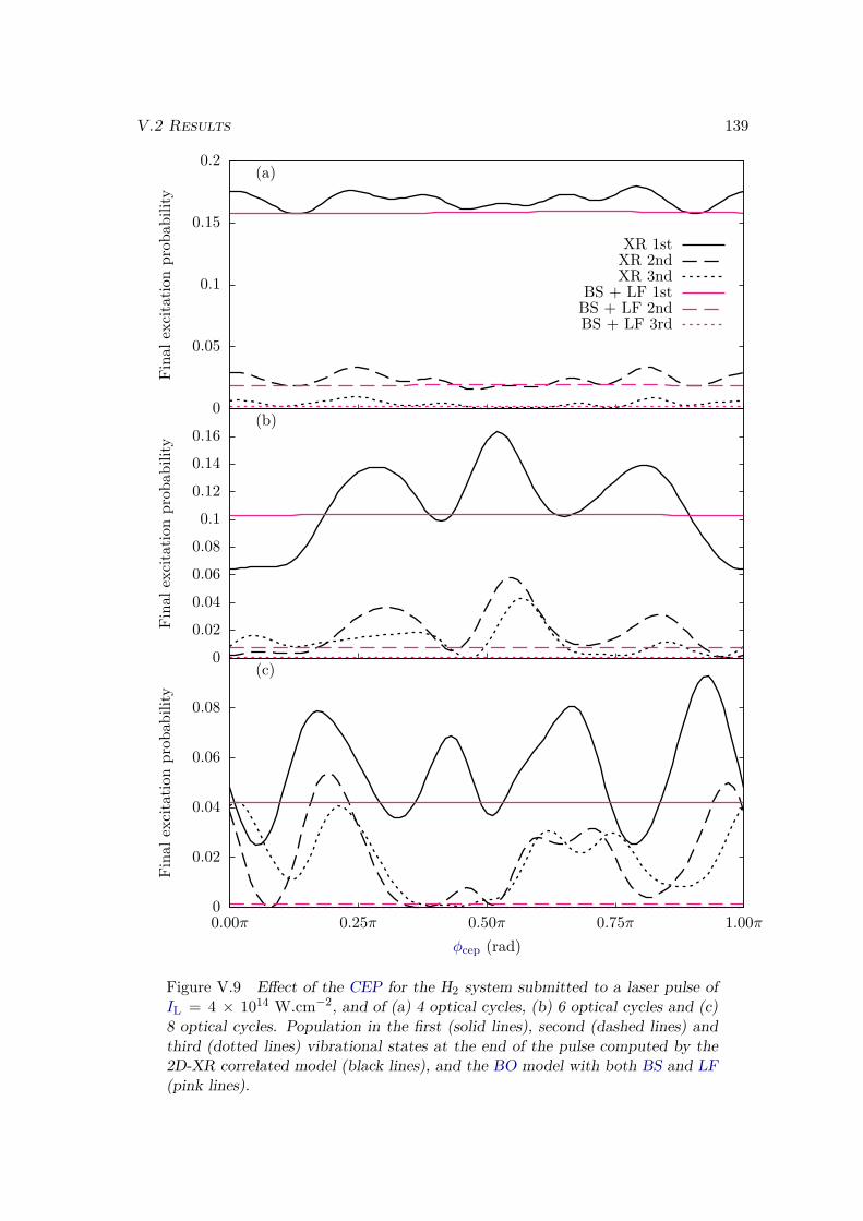
V.2 Results 139
0
0.05
0.1
0.15
0.2(a)
00.020.040.060.080.1
0.120.140.16
(b)
0
0.02
0.04
0.06
0.08
0.00π 0.25π 0.50π 0.75π 1.00π
(c)
Fina
lexcita
tionprob
ability
XR 1stXR 2ndXR 3nd
BS + LF 1stBS + LF 2ndBS + LF 3rd
Fina
lexcita
tionprob
ability
Fina
lexcita
tionprob
ability
φcep (rad)
Figure V.9 Effect of the CEP for the H2 system submitted to a laser pulse ofIL = 4 × 10¹⁴ W.cm−2, and of (a) 4 optical cycles, (b) 6 optical cycles and (c)8 optical cycles. Population in the first (solid lines), second (dashed lines) andthird (dotted lines) vibrational states at the end of the pulse computed by the2D-XR correlated model (black lines), and the BO model with both BS and LF(pink lines).
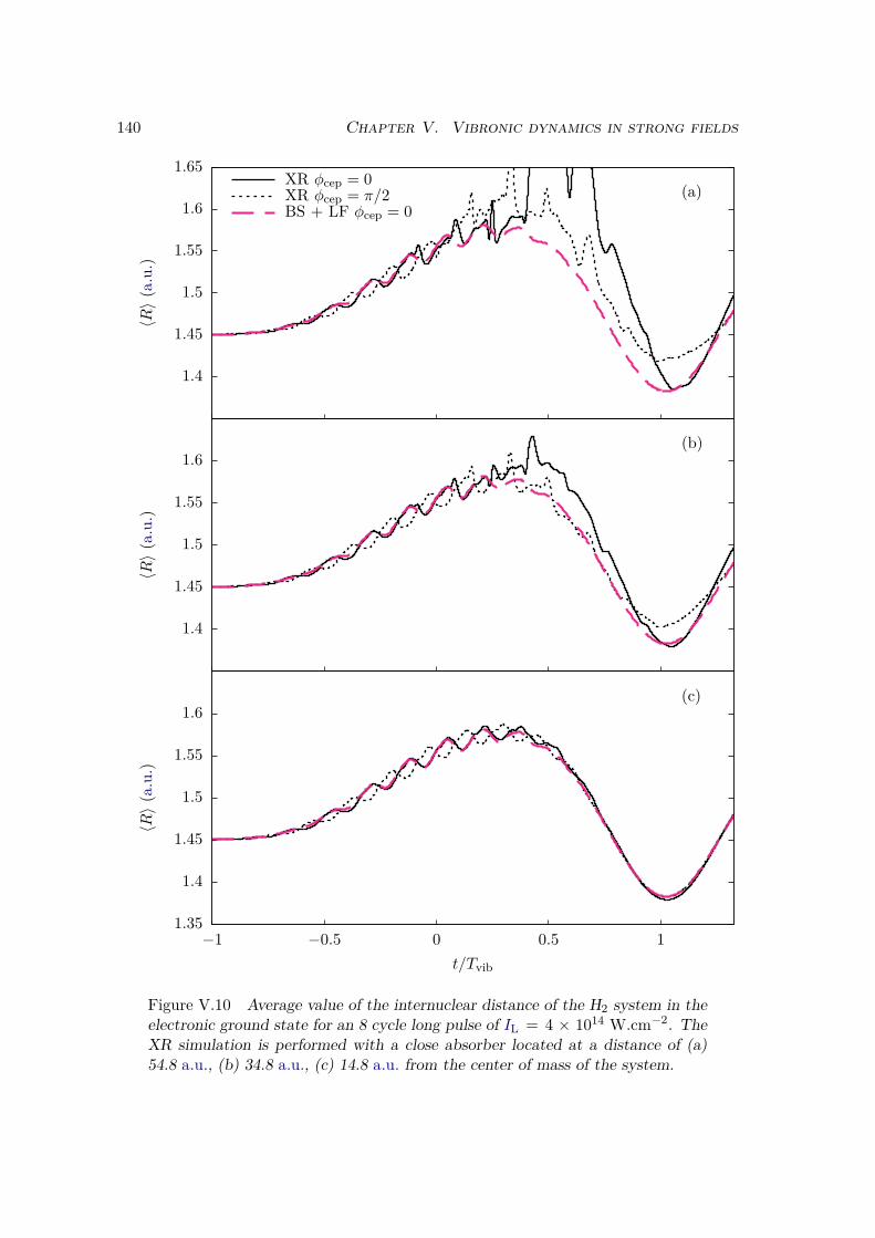
140 Chapter V. Vibronic dynamics in strong fields
1.4
1.45
1.5
1.55
1.6
1.65(a)
1.4
1.45
1.5
1.55
1.6(b)
1.35
1.4
1.45
1.5
1.55
1.6
−1 −0.5 0 0.5 1
(c)
〈R〉(a.u.)
XR φcep = 0XR φcep = π/2BS + LF φcep = 0
〈R〉(a.u.)
〈R〉(a.u.)
t/Tvib
Figure V.10 Average value of the internuclear distance of the H2 system in theelectronic ground state for an 8 cycle long pulse of IL = 4 × 10¹⁴ W.cm−2. TheXR simulation is performed with a close absorber located at a distance of (a)54.8 a.u., (b) 34.8 a.u., (c) 14.8 a.u. from the center of mass of the system.
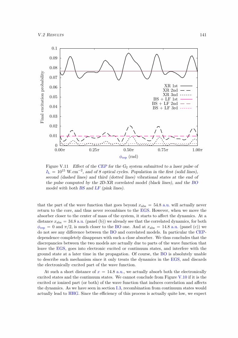
V.2 Results 141
0
0.01
0.02
0.03
0.04
0.05
0.06
0.07
0.08
0.09
0.1
0.00π 0.25π 0.50π 0.75π 1.00π
Fina
lexcita
tionprob
ability
φcep (rad)
XR 1stXR 2ndXR 3nd
BS + LF 1stBS + LF 2ndBS + LF 3rd
Figure V.11 Effect of the CEP for the G2 system submitted to a laser pulse ofIL = 1015 W.cm−2, and of 8 optical cycles. Population in the first (solid lines),second (dashed lines) and third (dotted lines) vibrational states at the end ofthe pulse computed by the 2D-XR correlated model (black lines), and the BOmodel with both BS and LF (pink lines).
that the part of the wave function that goes beyond xabs = 54.8 a.u. will actually neverreturn to the core, and thus never recombines to the EGS. However, when we move theabsorber closer to the center of mass of the system, it starts to affect the dynamics. At adistance xabs = 34.8 a.u. (panel (b)) we already see that the correlated dynamics, for bothφcep = 0 and π/2, is much closer to the BO one. And at xabs = 14.8 a.u. (panel (c)) wedo not see any difference between the BO and correlated models. In particular the CEP-dependence completely disappears with such a close absorber. We thus concludes that thediscrepancies between the two models are actually due to parts of the wave function thatleave the EGS, goes into electronic excited or continuum states, and interfere with theground state at a later time in the propagation. Of course, the BO is absolutely unableto describe such mechanism since it only treats the dynamics in the EGS, and discardsthe electronically excited part of the wave function.
At such a short distance of x = 14.8 a.u., we actually absorb both the electronicallyexcited states and the continuum states. We cannot conclude from Figure V.10 if it is theexcited or ionized part (or both) of the wave function that induces correlation and affectsthe dynamics. As we have seen in section I.3, recombination from continuum states wouldactually lead to HHG. Since the efficiency of this process is actually quite low, we expect
142 Chapter V. Vibronic dynamics in strong fields
intuitively that it is mainly the recombination from electronic bound excited states thatwill induce the correlated effects that we have observed. To investigate this, we considerthe G2 model system, which has only two electronic bound states. We thus kill mostof the excited states’ influence and concentrate on the continuum states. As we did forH2 in Figure V.9, we plot on Figure V.11 the population in the first vibrational statesat the end of the laser pulse as a function of the CEP for the G2 system. Since theG2 system has a lower ionization rate than our H2 system, we chose a higher intensity ofIL = 1015 W.cm−2 to reach similar ionization probability at the end of the pulse. Similarlyto the H2 model, we observe that the final populations oscillate with φcep, indicating thatwe did not kill all the correlation by "removing" most of the electronic excited states. Theamplitude of these oscillations is however much lower than in the case of H2, indicatingthat the electronic excitation indeed does play a major role. Nevertheless, the fact thatwe sill observe discrepancies with the BO model suggests that the continuum states arenot spectators, but also impact the nuclear dynamics.
To conclude, these results do not allow to fully understand the origin of the CEP-dependency in the nuclear dynamics. Since the continuum states seem to play a role inthis respect, it may be related to interference between the wave packets that are emittedat each half cycle of the laser field as described in [114]. However more work is needed todiscriminate between the effects of the electronic excited and continuum states.
V.3 Analytic derivation
To better understand the discrepancies between the BO and the fully correlated mod-els, we propose an analytical derivation of the BO nuclear TDSE based on the Wigner-Weisskopf approach. This method is a very general way to model a quantum system ininteraction with an environment. Since we are only interested in the system, we wantto separate its dynamics from this environment. This separation relies on the hypothesisthat the environment does not keep any memory of its interaction with the system, i.e.that any information is lost as soon as it reaches this environment. We follow the deriva-tion as it is performed in [78] for a two-level system, and we adapt it to the case of amolecule in a classical EM field. In our case, the system is the electronic ground state ofour neutral molecule, and the environment is composed of all the electronic excited andcontinuum states. In a first approach we concentrate on the BS mechanism, so that weonly consider the electronic bound states of the molecule, and not the continuum states.The wave function is decomposed on the vibrational states
∣∣∣v(i)j
⟩of all the electronic
states |ϕi〉 of the neutral molecule:
|ψ(t)〉 =∑i,j
ai,j(t)∣∣∣ϕi, v(i)
j
⟩; (V.18)
In the case of homonuclear diatomic molecules, the electric field does not couple thevibrational states within a given electronic state:
⟨ϕi, v
(i)j
∣∣∣µ · FL∣∣∣ϕi, v(i)
l
⟩= 0. (V.19)
V.3 Analytic derivation 143
Since we want to focus on the dynamics in the ground state, we also assume that we canneglect the coupling between electronic excited states:⟨
ϕi, v(i)j
∣∣∣µ · FL∣∣∣ϕk, v(k)
l
⟩= 0, if i, k ≥ 1. (V.20)
The Hamiltonian can be decomposed into blocks Hi,j corresponding to each electronicstate:
H =
H1,1 H1,2 H1,3 . . .H2,1 H2,2 0 . . . 0H3,1 0 H3,3 0
......
... . . .
(V.21)
where the diagonal blocs are diagonal matrices of the vibrational energies:
Hi,i =
ωi,1 0 . . .
0 ωi,2. . .
... . . .
(V.22)
and where the non diagonal blocks contains the couplings between the vibrational stateswithin the ground and electronic excited states:
H1,k =
V1,1,k V1,2,k . . .
V2,1,k V2,2,k. . .
... . . .
(V.23)
with
Vj,k,l(t) = −⟨ϕ0, v
(0)j
∣∣∣µ · FL(t)∣∣∣ϕk, v(k)
l
⟩(V.24)
= −FL2(eiωLt + e−iωLt
) ⟨ϕ0, v
(0)j
∣∣∣µz ∣∣∣ϕk, v(k)l
⟩. (V.25)
The coefficients ai,j(t) obey the following differential equations:
da0,jdt (t) = −iω0,ja0,j(t)− i
∑k>0,l
Vj,k,l(t)ak,l(t) (V.26)
dak,ldt (t) = −iωk,lak,l(t)− i
∑j
V ∗j,k,l(t)a0,j(t), if k > 0; (V.27)
For k 6= 0, the coefficients ak,l can be formally computed as:
ak,l(t) = −i∑m
∫ t
0dt′V ∗m,k,l(t′) eiωk,l(t′−t) a0,m(t′). (V.28)
144 Chapter V. Vibronic dynamics in strong fields
Inserting this expression in (V.26), and defining a0,j(t) = a0,j(t) eiω0,jt, we get:
da0,jdt (t) =−
∑k>0,l,m
ei(ω0,j−ω0,m)t∫ t
0dt′Vj,k,l(t)V ∗m,k,l(t′) ei(ωk,l−ω0,m)(t′−t) a0,m(t′) (V.29)
=− F 2L
2 cosωLt∑α=±1
∑k>0,l,m
⟨ϕ0, v
(0)j
∣∣∣µz ∣∣∣ϕk, v(k)l
⟩⟨ϕk, v
(k)l
∣∣∣µz ∣∣∣ϕ0, v(0)m
⟩×∫ t
0dt′ ei(ωk,l−ω0,m+αωL)(t′−t) a0,m(t′) (V.30)
=− F 2L
2 cosωLt∑α=±1
ei(ω0,j−ω0,m+αωL)t∫ t
0Nl,m,α(τ)a0,m(t− τ)dτ, (V.31)
where we changed the integration variable from t′ to τ = t− t′, and where we defined
Nl,m,α(τ) =∑
k>0,l,m
⟨ϕ0, v
(0)j
∣∣∣µz ∣∣∣ϕk, v(k)l
⟩⟨ϕk, v
(k)l
∣∣∣µz ∣∣∣ϕ0, v(0)m
⟩e−i(ωk,l−ω0,m+αωL)τ .
(V.32)
In the Wigner-Weisskopf approach, this Nl,m,α(τ) term is considered to be very close toa Dirac delta function:∫ t
0Nl,m,α(τ)a0,m(t− τ)dτ ' a0,m(t)
∫ ∞0Nl,m,α(τ)dτ. (V.33)
One can find different way to interpret this assumption. First we can consider the sumover k as a sum of terms of very different frequencies ωk,l and similar amplitude. Thedifferent frequencies of this sum thus get very quickly out of phase as soon as τ & 1/ω0,m.This is referred to as the Markov approximation, and interpreted as a zero memory timeof the "reservoir" made of the electronic excited states. Equivalently, it means that theelectron is lost as soon as it is promoted to an excited state, i.e. to the reservoir, and thereservoir keeps no memory of having received this electron. The interpretation makes useof the Saddle Point Approximation on the integral over τ :∫ t
0e−i(ωk,l−ω0,m+αωL)τ a0,m(t− τ)dτ ' a0,m(t)
∫ ∞0
e−i(ωk,l−ω0,m+αωL)τ dτ. (V.34)
Since there is only one saddle point at τ = 0, we get the following orders:∫ t
0e−i(ωk,l−ω0,m+αωL)τ a0,m(t− τ)dτ ' a0,m(t)
∫ ∞0
dτ e−i(ωk,l−ω0,m+αωL)τ
− da0,mdt (t)
∫ ∞0
τ e−i(ωk,l−ω0,m+αωL)τ dτ + ... (V.35)
= a0,m(t)(πδ(ω0,m − ωk,l − αωL) + iPP 1
ω0,m − ωk,l − αωL
)
+ da0,mdt (t)
(iπδ′(ω0,m − ωk,l − αωL) + PP 1
(ω0,m − ωk,l − αωL)2
)+ ... (V.36)
V.3 Analytic derivation 145
where PP indicates that we consider the Cauchy principal value of the enclosed ex-pression, and δ, δ′, ... are the Dirac delta function and its derivatives. We can now insertthis in (V.31) to get:da0,j
dt (t) = −∑m
ei(ω0,j−ω0,m)t[a0,m(t)
(Γj,m(t)2 + i∆j,m(t)
)+ da0,m
dt (t)(Θj,m(t) + i Ξj,m(t)
)](V.37)
where
Γj,m(t) =πF 2L
2 cos(ωLt)∑α=±1
eiαωLt
×∑k>0,l
⟨ϕ0, v
(0)j
∣∣∣µz ∣∣∣ϕk, v(k)l
⟩⟨ϕk, v
(k)l
∣∣∣µz ∣∣∣ϕ0, v(0)m
⟩δ(ω0,m − ωk,l − αωL)
(V.38)
∆j,m(t) =F 2L
2 cos(ωLt)∑α=±1
eiαωLt
×∑k>0,l
⟨ϕ0, v
(0)j
∣∣∣µz ∣∣∣ϕk, v(k)l
⟩⟨ϕk, v
(k)l
∣∣∣µz ∣∣∣ϕ0, v(0)m
⟩PP 1
ω0,m − ωk,l − αωL(V.39)
Θj,m =F 2L
2 cos(ωLt)∑α=±1
eiαωLt
×∑k>0,l
⟨ϕ0, v
(0)j
∣∣∣µz ∣∣∣ϕk, v(k)l
⟩⟨ϕk, v
(k)l
∣∣∣µz ∣∣∣ϕ0, v(0)m
⟩PP 1
(ω0,m − ωk,l − αωL)2
(V.40)
Ξj,m =− πF 2L
2 cos(ωLt)∑α=±1
eiαωLt
×∑k>0,l
⟨ϕ0, v
(0)j
∣∣∣µz ∣∣∣ϕk, v(k)l
⟩⟨ϕk, v
(k)l
∣∣∣µz ∣∣∣ϕ0, v(0)m
⟩δ′(ω0,m − ωk,l − αωL).
(V.41)In the adiabatic approximation, the laser frequency can be considered very small withrespect to all the energy gaps ωk,l − ω0,m. We can thus neglect the Γj,m and the Ξj,m,and approximate the ∆j,m (V.39) and Θj,m (V.40) by
∆j,m(t) =F 2L cos2(ωLt)
∑k>0,l
⟨ϕ0, v
(0)j
∣∣∣µz ∣∣∣ϕk, v(k)l
⟩⟨ϕk, v
(k)l
∣∣∣µz ∣∣∣ϕ0, v(0)m
⟩ω0,m − ωk,l
(V.42)
Θj,m =F 2L cos2(ωLt)
∑k>0,l
⟨ϕ0, v
(0)j
∣∣∣µz ∣∣∣ϕk, v(k)l
⟩⟨ϕk, v
(k)l
∣∣∣µz ∣∣∣ϕ0, v(0)m
⟩(ω0,m − ωk,l)2 (V.43)
If we only keep the first order of the SPA (i.e. the ∆j,m terms) then we find the followingdifferential equations for the a0,j :
ida0,jdt (t) = ω0,ja0,j(t) +
∑m
∆j,m(t)a0,m(t). (V.44)
146 Chapter V. Vibronic dynamics in strong fields
This is a new Schrödinger equation that describes the dynamics of the nuclear wave packeton the electronic ground state of the neutral molecule. The additional term ∆ couples thedifferent vibrational states of the electronic ground state through the interaction with theelectronic excited states. This is the term responsible for the Bond-Softening mechanism.To recover the expression that we used in the previous section, we still need to neglectthe differences between the vibrational energies with respect to the electronic energies Ekand get
∆j,m(t) = F 2L cos2(ωLt)
∑k>0,l
⟨ϕ0, v
(0)j
∣∣∣µz ∣∣∣ϕk, v(k)l
⟩⟨ϕk, v
(k)l
∣∣∣µz ∣∣∣ϕ0, v(0)m
⟩E0 − Ek
. (V.45)
Lastly we suppose that we can write the vibronic states |Nk,l, ϕk〉 as BO products ϕk(r; R)χk,l(R),so that we can use the identity closure relation 1 = ∑
l |Nk,l〉 〈Nk,l| for each electronicstate k:
∆j,m(t) =F 2L cos2(ωLt)
⟨v
(0)j
∣∣∣∑k>0
|〈ϕ0(r; R)|µz |ϕk(r; R)〉r|2
E0 − Ek
∣∣∣v(0)m
⟩. (V.46)
where 〈|〉r indicates that we only integrate over r. We recognize the expression of thesecond order Stark shift [135]. Using the expression of the polarizability:
α(R) =∑k>0
|〈ϕ0(r; R)|µz |ϕk(r; R)〉r|2
Ek − E0, (V.47)
the expression of the matrix ∆ finally reduces to
∆ = −α(R)F 2L cos2(ωLt). (V.48)
We thus find that the matrix ∆ is equal to the statical R-dependent Stark shift, where wereplaced the value of the static field by the time-dependent laser electric field. The factthat we only find the first non zero order of perturbation theory (i.e. the polarizability)for the Stark shift is a direct consequence of the approximation made in neglecting thecoupling between electronic excited states. Indeed these couplings appear in the expressionof the higher order terms [135].
If we include the following order of the SPA, i.e. the Θ matrix, we find additionalterms. We apply the same approximations we just used for ∆ to the Θ matrix to find:
Θ = F 2L cos2(ωLt)
∑k>0,l
|〈ϕ0(r; R)|µz |ϕk(r; R)〉r|2
(E0 − Ek)2 . (V.49)
We denote by A0 the vector of coefficients a0,j in order to write (V.31) under matrix form:
idA0dt (t) = [H + ∆]A0(t)− iΘdA0
dt (t) (V.50)
= [1 + Θ]−1 [H + ∆]A0(t). (V.51)
We conclude that the nuclear wave packet in the electronic ground state evolves under theperturbed Hamiltonian [1 + Θ]−1 [H + ∆]. This Hamiltonian includes corrections that
V.3 Analytic derivation 147
describe the above mentioned memory of the "reservoir". It would thus be interestingto test if it can reproduce the recombinations, and the CEP-dependency, that we haveobserved in the previous section and that were not included in the first order equation(V.44). However we did not have time to perform the corresponding simulations, andleave this here as an open perspective.
We recovered the TDSE for the NWP in the electronic ground state for the BS mech-anism. If we want to include the LF we need to add the electronic states of the ionizedspecies to our initial description of the wave function (V.18):
|ψ(t)〉 =∑i,j
ai,j(t)∣∣∣ϕi, v(i)
j
⟩+∑l
∫dEdβ ρ(E)bl(E, β, t) |E, β〉
∣∣∣v+l
⟩, (V.52)
where the∣∣∣v+l
⟩refer to the vibrational states of the cationic molecule with energy ω+,l, and
E is the energy of the ionized electron, and β a set of quantum numbers (see section I.1).We can perform the same Wigner-Weisskopf derivation with such an ansatz. We will findthe same modified differential equations (V.31) for the coefficients a0,j , but the expressionof the Γ, ∆, Θ and Ξ matrices will be changed. We only give here the expression of theΓ terms:
Γj,m(t) =πF 2L
2 cos(ωLt)∑α=±1
eiαωLt
×[ ∑k>0,l
⟨ϕ0, v
(0)j
∣∣∣µz ∣∣∣ϕk, v(k)l
⟩⟨ϕk, v
(k)l
∣∣∣µz ∣∣∣ϕ0, v(0)m
⟩δ(ω0,m − ωk,l − αωL)
+∑l
ρ(E)∫
dβ⟨ϕ0, v
(0)j
∣∣∣µz ∣∣∣E, β, v+l
⟩⟨E, β, v+
l
∣∣∣µz ∣∣∣ϕ0, v(0)m
⟩ ∣∣∣∣E=ω0,m−ω+,l−αωL
].
(V.53)
Compared to the previous expression (V.38), we get new terms (on the third line) thatcorrespond to the interaction of the vibrational states mediated through the contin-uum states. Moreover, those terms form an (almost) anti-Hermitian matrix, exactlylike the −iΓ(R,FL(t)) matrix that we used for the BO model (see section V.1.2). Itis thus highly tempting to conclude that it is the matrix that is responsible for theLochfraß mechanism. Nevertheless, as before, we see from the energy conservation rela-tion E = ω0,m − ω+,l − αωL, which can also be written ωL = ±(E + ω+,l − ω0,m), thatthe photon energy has to match the energy difference between the vibrational state
∣∣∣v(0)j
⟩and the mediating continuum state |E, β〉. Or, said otherwise, we only get the first nonzero order of perturbation theory. This is somewhat expected from what we just saidwith the previous derivation: we cannot describe multiphoton transitions from the elec-tronic ground state to the continuum if we do not couple the continuum states betweenthemselves. In the case of BS this has minimal consequences because the first non zeroorder of perturbation theory is actually the dominant one. On the contrary, for the LFmechanism it is crucial to have all the higher orders to describe tunnel ionization. Wethus need to include couplings between the continuum states. Unfortunately we also haveto leave this part of the calculation as a perspective.
148 Chapter V. Vibronic dynamics in strong fields
V.4 ConclusionWe have studied ultrafast correlated vibrational dynamics in small homonuclear diatomicmolecules initiated by strong femtosecond IR laser pulses. We have tested the relevanceof the commonly accepted Lochfraß/Bond-Softening interpretations of these dynamics.We showed that this dichotomy is actually highly limited since it erroneously supposesthat the two mechanisms are decoupled. As a consequence, the previously used modelswhere one consider only one of the two excitation mechanisms (BS or LF) leads to un-physical interpretations of the system dynamics. Since the two mechanisms are coupled,they actually have to be included simultaneously in the model to get correct results. Inparticular we showed that the information contained in the phase of the nuclear wavepacket oscillations was more delicate to interpret than predicted in [222, 223, 227].
Moreover we investigated the influence of the vibronic correlation on the dynamics.We found that this correlation has minimal consequences for low intensity and very shortlaser pulses. On the contrary for high intensity and longer pulses, we found that wecould not neglect the part of the wave function that left the electronic ground state andrecombines with it later on. This recombination is a correlated process that is completelyabsent of the Born-Oppenheimer model. Our correlated numerical results indicate thatit induces excitation in higher vibrational levels and is strongly dependent on the carrierenvelop phase of the laser pulse. This CEP-dependency could be used as a signature ofvibronic correlations in experimental measurements. We could not manage to identifythe mechanism which explains this CEP-dependency. Our results with a short-rangepotential indicates that the recombination processes occurs mainly from the electronicexcited states, but that the contribution of the continuum states, i.e. the ionized part ofthe wave function, cannot be neglected either. More work is required to further concludeon which electronic states are involved in the vibronic correlations.
Finally we derived the expression of the Bond-Softening term that appears in thenuclear TDSE using the Wigner-Weisskopf approach. We found a correction term thatmay allow to include some correlation while keeping a BO description of the wave function.More simulations are needed to determine to what extent it contributes. We could notdirectly apply the same approach for the Lochfraß term since the couplings between thecontinuum states have to be taken into account.
Chapter VI
Time-Dependent Configuration Inter-action
In the previous chapters, we have studied the response of atomic and molecular systems tointense and ultrashort laser pulses. In many cases, reaching a clear understanding of themechanisms that govern the electron dynamics is still a challenge that requires advancedtheory [164]. It is therefore crucial to develop theoretical and computational methodscapable of providing precise treatments of the fundamental electronic processes generatedby a strong laser field [228–231]. To achieve this goal we can rely on two complementaryapproaches: accurate numerical calculations to get quantitative results, and approximateor simplified models to get more qualitative quantities but valuable physical insight. Inthe previous chapters we concentrated on the latter. Our strategy was either to developapproximate analytical models, or to consider simple systems with low dimensions, forwhich an intensive numerical treatment is possible. As we saw, this qualitative approachis very powerful because it allows to develop physical interpretations. In this chapterwe follow the other approach: we investigate numerical methods that would be able todescribe larger and more complex system.
In strong field physics, the most numerically accurate computational approaches usu-ally rely on the Single Active Electron (SAE) approximation. This supposes that only oneelectron participates to the dynamics, and that all the other electrons remain "frozen".Indeed, we have seen in Chapter I that highly non-linear processes are initiated whentunnel ionization is induced by the laser electric field. This effect depends exponentiallyon the potential energy barrier, and thus on the energy of the orbital from which theelectron is ionized: the deeper the orbital, the more difficult it is for the electron to tun-nel out. For atomic systems the orbitals are in general sufficiently separated in energyso that only the highest one gets ionized, leaving the ion in its ground state. We canthus discard the electronic dynamics in the ion, and only describe the ionized electron.However, this approximation is not always justified. In Xenon it has been showed that thereturning electron may interact with the electrons of the ion, leading to an extension ofthe HHG cutoff relative to the SAE predictions [232, 233] which has been experimentallymeasured [49]. In the case of molecules the energy differences between the Highest Occu-pied Molecular Orbital (HOMO) and the inner-valence orbitals (the so-called HOMO-1,HOMO-2...) is in general smaller than for atoms. In this case, several orbitals may be
149
150 Chapter VI. Time-Dependent Configuration Interaction
ionized, leaving the ion in several excited states. The relative importance of these ioniza-tion channels will depend on the orbital geometry and on the orientation of the moleculewith respect to the field. In the particular case of HHG, each ionization channel leads toa quantum path with the same initial and final states, so that they may interfere, and theinterference signature could be seen in the emitted spectrum. Such interferences have beenexperimentally measured and used to retrieve the dynamics of the hole in the molecularion [50, 234]. Obviously the computational methods based on the SAE approximationcannot account for such multi-electron effects.
Nowadays, the multi-electron dynamics problem in strong laser fields is tackled bytwo main families of theoretical methods: Time-Dependent Density Functional Theory(TDDFT) and time-dependent wave-function methods [164, 235–239]. Most developmentsin these approaches focus on the accurate description of electron correlation. However,because of the complexity of non-linear optical phenomena, such as HHG and ATI, anothercrucial aspect needs to be carefully addressed: the choice of the one-electron basis setfor representing the time-dependent wave function involved in these models. In fact, areliable description of the electron dynamics in strong laser fields depends on the accuracyin reproducing the bound states and, more importantly, the continuum states of themolecule. In addition, choosing a "good" basis set can improve the numerical convergenceof the results and reduce the computational cost of simulations.
Most of the proposed numerical methods in the literature directly describe the sys-tem wave function on a real-space grid [10, 240–242] or through a numerically definedgrid-based basis set of functions, as in the case of the discrete-variable representationmethod [141], the pseudospectral grid method, or the finite-element method [243]. Withinthese approaches, new schemes have been proposed to compute ATI spectra in molecules[244] and to study the different molecular orbital contributions to HHG spectra [245, 246].Grid-based basis sets have demonstrated to be very efficient to describe non-linear opticalphenomena. However, the computational cost can be very high and the development ofstrategies involving multi-level parallelization schemes for massively parallel simulationshave been necessary [247].
Another recurrent basis set in the context of ultrafast electron dynamics is composedof B-splines, defined as piecewise polynomial functions with compact support [248]. Theywere first introduced in atomic calculations by B. Shore [249] and later extensively used totreat ionized and excited states [250, 251]. B-splines have proved to be a very powerful toolto describe multiphoton ionization processes in atoms and molecules in the frameworksof TDDFT and wave-function methods [252, 149, 253, 254]. The success of B-splines isdue to a remarkable feature: B-splines can reproduce accurately and simultaneously bothbound and continuum states. This numerical property is directly related to their effectivecompleteness [255]. Today atomic packages based on B-splines are available [256–258] andrecent studies show their ability to reproduce HHG and ATI spectra of molecules underthe action of strong laser fields [259]. However, new algorithms have to be developedin order to increase the computational efficiency of calculations with B-splines for largersystems.
More recently, Gaussian-type orbital functions (abbreviated as Gaussian functions inthe following), that extensively proved their efficiency for the computation of the boundstate of many different chemical species, have been used to calculate HHG spectra in atomsand molecules in the framework of the Time-Dependent Configuration Interaction (TDCI)
151
method [260, 235, 261, 262]. The importance of diffuse basis functions and multi-centeredbasis functions to improve continuum states was pointed out [260, 235]. Alternatively,Gaussian functions with exponents optimized to improve the description of the continuumstates have been used in the case of the H and He atoms [261, 263]. This latter strategyhas lower computational cost, although it remains to be tested on molecular systems.
Finally, to overcome some of the limitations of the grid, B-splines, and Gaussianbasis sets, hybrid basis sets have been proposed in recent years. Gaussian functionswere used together with grid-based functions to reproduce electron dynamics in molecularsystems [264], and Gaussian functions have also been combined with B-splines for studyingionization of H and He atoms [265, 266].
In this work, performed in collaboration with Felipe Zapata Abellán, Emanuele Coccia,Julien Toulouse, Valérie Véniard and Eleonora Luppi from the Laboratoire de ChimieThéorique at Sorbonne Université, we compare the performance of the three families ofbasis sets briefly reviewed above, i.e. Grid, B-splines, and Gaussians, for the calculation ofHHG and ATI spectra of the molecular ion H+
2 . This benchmark system has been chosenbecause it has the advantage of having only one electron, which allows us not to bias ourinvestigation with possible effects due to electron correlation. Indeed, with this simplecase, we can focus on the effectiveness of the representation of the continuum states forthe electron dynamics and the computational advantages of each basis set. Moreover, thepresence of two nuclei in H+
2 offers the opportunity to observe intricate physical features,such as quantum interferences in the HHG process [267, 268, 200] as we saw in Chapter IV.In this case we were able to perform calculations in 1D as well as in 3D. The 3D results,obtained by Emanuale Coccia and Eleonora Luppi will not be presented here.
We then investigate the perspective of generalization of the grid and Gaussian methodsto bielectronic systems. In particular we study the ability of the TDCI method, developedin [235], to reproduce the HHG spectrum of the H2 molecule and of the Helium atom,by comparing its predictions with converged results obtained on a bidimensional grid.In the present work we only did 1D simulations. Indeed, even the bidimensional gridcalculations already needed to run for a few tens of hours to get converged results, so that3D calculations were unreachable. In contrast, the Gaussian-based TDCI simulationsonly lasted a few minutes, which highlights why the latter method seems promising forthe description of even larger systems.
Note that, as mentioned above, we will test that ability of the different method toreproduce the continuum states of the system. However, all these numerical models relyon a discretization of the Hilbert space, so that, as detailed for the real-space grid insection II.1.1, the spectrum of the discretized Hamiltonian do not present a real "contin-uum". Nevertheless, through misuse of language, we will call "continuum" the positiveenergy part of the spectrum.
Objectives
ü Find a computational method able to accurately describe multi-electron systems instrong fields.
ü Investigate the basis set on which to develop such a method.
ü Test the ability of the TDCI method to reproduce the HHG spectrum of bielectronic
152 Chapter VI. Time-Dependent Configuration Interaction
systems.
VI.1 One dimensional theoretical model of H+2
Our 1D model of H+2 is defined by a molecular Soft-Coulomb potential (II.2) (see sec-
tion II.1.1). The regularization parameter a is chosen to reproduce the ionization poten-tial Ip = 30 a.u. of the real H+
2 molecule at a given value of the internuclear distance R(a = 1.2 a.u. at Req = 2.0 a.u.) [211]. HHG spectra were obtained from the solution ofthe discretized TDSE via the Fourier transform of the average value of the accelerationas depicted in section II.3.2, and ATI spectra were obtained with the Window method asdetailed in section II.3.4.
VI.1.1 Real-space Grid
As in the previous chapters, and as described in section II.1.1, the 1D time-dependentwave function is discretized on a real-space grid of Nx points xi separated by a constantstep ∆x. It is thus represented by the vector
|ψ(t)〉 ≡ (ψ(x1, t), . . . , ψ(xi, t), . . . , ψ(xN , t)). (VI.1)
The TDSE is solved by means of the Crank-Nicolson propagation algorithm [83] (seesection II.1.2 b)). The H+
2 ground state computed by inverse iteration [137] (see sec-tion II.1.3) is taken as the initial state in the propagation. In addition, to avoid unphysicalreflections at the boundaries of the simulation grid, a mask-type absorber function [143]was implemented with a spatial extension of habs = 50 a.u. (see section II.1.1 c)).
For ATI spectra, converged results were obtained withNx = 200001 and ∆x = 0.02 a.u.,and with a time step ∆t = 8.41 × 10⁻⁴ a.u.. For HHG spectra, we obtained convergedresults with Nx = 160001, ∆x = 0.01 a.u., and ∆t = 1.35× 10⁻² a.u..
VI.1.2 B-spline basis set
These calculations were performed by Felipe Zapata Abellán during his PhD at the Lab-oratoire de Chimie Théorique at Sorbonne Université, and we are grateful to be allowedto present his results here.
The time-dependent wave function with the B-spline basis set is represented as
ψ(x, t) =M∑i=1
ci(t)Bki (x), (VI.2)
where ci(t) are time-dependent coefficients and Bki (x) are B-spline functions of order k
and dimension M . The B-spline, Bki (x), is a piecewise polynomial of degree k− 1 defined
inside an interval of the support grid Xi ≤ x ≤ Xi+k and which vanishes outsidethis interval. The end-points of the support grid are chosen to be k-fold degenerate :X1 = X2 = . . . = Xk = Xmin and XM+1 = XM+2 = . . . = XM+k = Xmax and fornon-degenerate grid points the width of the interval is Xi+1 − Xi = Xmax/(M − k + 1)[149].
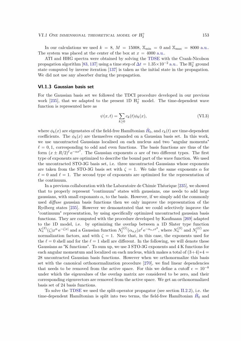
VI.1 One dimensional theoretical model of H+2 153
In our calculations we used k = 8, M = 15008, Xmin = 0 and Xmax = 8000 a.u..The system was placed at the center of the box at x = 4000 a.u..
ATI and HHG spectra were obtained by solving the TDSE with the Crank-Nicolsonpropagation algorithm [83, 137] using a time step of ∆t = 1.35×10⁻² a.u.. The H+
2 groundstate computed by inverse iteration [137] is taken as the initial state in the propagation.We did not use any absorber during the propagation.
VI.1.3 Gaussian basis setFor the Gaussian basis set we followed the TDCI procedure developed in our previouswork [235], that we adapted to the present 1D H+
2 model. The time-dependent wavefunction is represented here as
ψ(x, t) =∑k≥0
ck(t)φk(x), (VI.3)
where φk(x) are eigenstates of the field-free Hamiltonian H0, and ck(t) are time-dependentcoefficients. The φk(x) are themselves expanded on a Gaussian basis set. In this work,we use uncontracted Gaussians localised on each nucleus and two "angular momenta"` = 0, 1, corresponding to odd and even functions. The basis functions are thus of theform (x ± R/2)` e−αx2 . The Gaussian exponents α are of two different types. The firsttype of exponents are optimized to describe the bound part of the wave function. We usedthe uncontracted STO-3G basis set, i.e. three uncontracted Gaussians whose exponentsare taken from the STO-3G basis set with ζ = 1. We take the same exponents α for` = 0 and ` = 1. The second type of exponents are optimized for the representation ofthe continuum.
In a previous collaboration with the Laboratoire de Chimie Théorique [235], we showedthat to properly represent "continuum" states with gaussians, one needs to add largegaussians, with small exponants α, to the basis. However, if we simply add the commonlyused diffuse gaussian basis functions then we only improve the representation of theRydberg states [235]. However we demonstrated that we could selectively improve the"continuum" representation, by using specifically optimized uncontracted gaussian basisfunctions. They are computed with the procedure developed by Kaufmann [269] adaptedto the 1D model, i.e. by optimizing the overlap between a 1D Slater type functionN
(S)n (ζ)xn e−ζ|x| and a Gaussian function N (G)
l (αn,`)x` e−αn,`x2 , where N (S)n and N (G)
l arenormalization factors, and with ζ = 1. Note that, in this case, the exponents used forthe ` = 0 shell and for the ` = 1 shell are different. In the following, we will denote theseGaussians as "K functions". To sum up, we use 3 STO-3G exponents and 4 K functions foreach angular momentum and localized on each nucleus, which makes a total of (3+4)∗4 =28 uncontracted Gaussian basis functions. However when we orthonormalize this basisset with the canonical orthonormalization procedure [270], we find linear dependenciesthat needs to be removed from the active space. For this we define a cutoff ε = 10−8
under which the eigenvalues of the overlap matrix are considered to be zero, and theircorresponding eigenvectors are removed from the active space. We get an orthonormalizedbasis set of 24 basis functions.
To solve the TDSE we used the split-operator propagator (see section II.2.2), i.e. thetime-dependent Hamiltonian is split into two terms, the field-free Hamiltonian H0 and
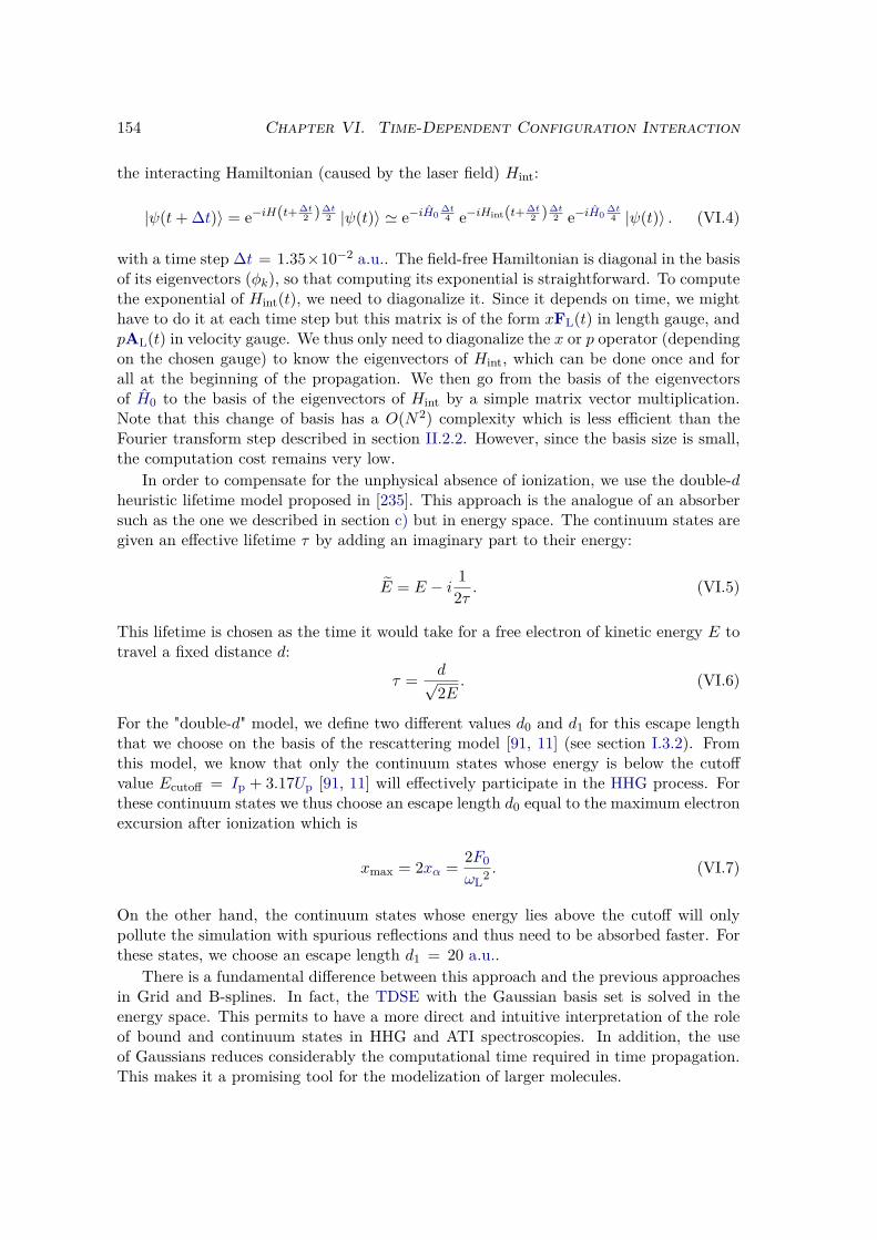
154 Chapter VI. Time-Dependent Configuration Interaction
the interacting Hamiltonian (caused by the laser field) Hint:
|ψ(t+ ∆t)〉 = e−iH(t+ ∆t2 )∆t
2 |ψ(t)〉 ' e−iH0∆t4 e−iHint(t+ ∆t
2 )∆t2 e−iH0
∆t4 |ψ(t)〉 . (VI.4)
with a time step ∆t = 1.35×10⁻² a.u.. The field-free Hamiltonian is diagonal in the basisof its eigenvectors (φk), so that computing its exponential is straightforward. To computethe exponential of Hint(t), we need to diagonalize it. Since it depends on time, we mighthave to do it at each time step but this matrix is of the form xFL(t) in length gauge, andpAL(t) in velocity gauge. We thus only need to diagonalize the x or p operator (dependingon the chosen gauge) to know the eigenvectors of Hint, which can be done once and forall at the beginning of the propagation. We then go from the basis of the eigenvectorsof H0 to the basis of the eigenvectors of Hint by a simple matrix vector multiplication.Note that this change of basis has a O(N2) complexity which is less efficient than theFourier transform step described in section II.2.2. However, since the basis size is small,the computation cost remains very low.
In order to compensate for the unphysical absence of ionization, we use the double-dheuristic lifetime model proposed in [235]. This approach is the analogue of an absorbersuch as the one we described in section c) but in energy space. The continuum states aregiven an effective lifetime τ by adding an imaginary part to their energy:
E = E − i 12τ . (VI.5)
This lifetime is chosen as the time it would take for a free electron of kinetic energy E totravel a fixed distance d:
τ = d√2E
. (VI.6)
For the "double-d" model, we define two different values d0 and d1 for this escape lengththat we choose on the basis of the rescattering model [91, 11] (see section I.3.2). Fromthis model, we know that only the continuum states whose energy is below the cutoffvalue Ecutoff = Ip + 3.17Up [91, 11] will effectively participate in the HHG process. Forthese continuum states we thus choose an escape length d0 equal to the maximum electronexcursion after ionization which is
xmax = 2xα = 2F0ωL2 . (VI.7)
On the other hand, the continuum states whose energy lies above the cutoff will onlypollute the simulation with spurious reflections and thus need to be absorbed faster. Forthese states, we choose an escape length d1 = 20 a.u..
There is a fundamental difference between this approach and the previous approachesin Grid and B-splines. In fact, the TDSE with the Gaussian basis set is solved in theenergy space. This permits to have a more direct and intuitive interpretation of the roleof bound and continuum states in HHG and ATI spectroscopies. In addition, the useof Gaussians reduces considerably the computational time required in time propagation.This makes it a promising tool for the modelization of larger molecules.
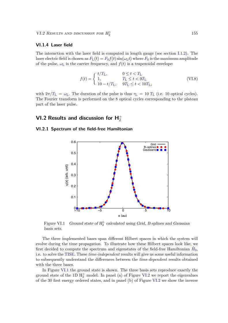
VI.2 Results and discussion for H+2 155
VI.1.4 Laser field
The interaction with the laser field is computed in length gauge (see section I.1.2). Thelaser electric field is chosen as FL(t) = F0f(t) sin(ωLt) where F0 is the maximum amplitudeof the pulse, ωL is the carrier frequency, and f(t) is a trapezoidal envelope:
f(t) = t/TL, 0 ≤ t < TL
1, TL ≤ t < 9TL10− t/TL, 9TL ≤ t < 10TL,
(VI.8)
with 2π/TL = ωL. The duration of the pulse is thus τL = 10 TL (i.e. 10 optical cycles).The Fourier transform is performed on the 8 optical cycles corresponding to the plateaupart of the laser pulse.
VI.2 Results and discussion for H+2
VI.2.1 Spectrum of the field-free Hamiltonian
0
0.1
0.2
0.3
0.4
0.5
0.6
−10 −5 0 5 10
ϕ(x
) (ar
b. u
nit)
x (au)
GridB−splinesGaussians
Figure VI.1 Ground state of H+2 calculated using Grid, B-splines and Gaussian
basis sets.
The three implemented bases span different Hilbert spaces in which the system willevolve during the time propagation. To illustrate how these Hilbert spaces look like, wefirst decided to compute the spectrum and eigenstates of the field-free Hamiltonian H0,i.e. to solve the TISE. These time-independent results will give us some useful informationto subsequently understand the differences between the time-dependent results obtainedwith the three bases.
In Figure VI.1 the ground state is shown. The three basis sets reproduce exactly theground state of the 1D H+
2 model. In panel (a) of Figure VI.2 we report the eigenvaluesof the 30 first energy ordered states, and in panel (b) of Figure VI.2 we show the inverse
156 Chapter VI. Time-Dependent Configuration Interaction
−2−1
012345678
0 5 10 15 20 25 30
(a)
0
1
2
3
4
5
6
0 0.1 0.2 0.3 0.4 0.5 0.6 0.7 0.8 0.9
(b)
E(a.u.)
State number
GridB-splinesGaussians
ρ−
1(a.u.)
E (a.u.)
GridB-splinesGaussians
Figure VI.2 (a) Eigenvalues up to the 30th eigenstate. (b) Inverse of the nor-malized density of continuum states.
of the density of the continuum states which is defined as
ρ(Ej) = 1Ej+1 − Ej
, (VI.9)
where Ej is a positive eigenvalue. In order to compare the three basis sets, the densityhas been normalized to the length of the simulation box in the case of Grid and B-splinesand to an arbitrary constant in the case of Gaussians. Since the three basis sets containa finite number of elements, the "continuum" part of the spectrum obviously contains afinite number of eigenstates. As we have seen in section II.1.1, the "continuum" computedon a grid is actually very close to the exact "continuum" of a free particle in a box, if weremain at low energies. We observe that this is also the case for the B-splines, and thatthere are virtually no differences between the grid and the B-splines results. Surprisinglythe density of states computed with the Gaussians is actually quite close to the one ofthe particle in a 25 a.u. box. However the number of "continuum" states is much lowerthat in the case of the Grid or the B-splines. This issue is a direct consequence of therelatively small size of the Gaussian basis set compared to the number of Grid or B-splines used. Indeed, the basis STO-3G+4K contains only 24 Gaussian basis functionswhereas we used 40001 grid points and 15000 B-splines. In principle, we could increase thenumber of Gaussians but this quickly leads to numerical instabilities, as will be discussedin section VI.2.3. This problem prevents us to use more than a few tens of optimizedGaussian functions. This fact, as we will see in the following sections, can have importantconsequences on the calculation of HHG and, in particular, of ATI spectra.
To investigate the accuracy of Grid, B-splines and Gaussian in the description ofthe "continuum" wave functions, we have chosen two "continuum" energies representativeof two different positive energy regions : low energy E = 0.06 a.u. and high energyE = 1.97 a.u.. For each of these energies, we reported in Figure VI.3 the correspond-
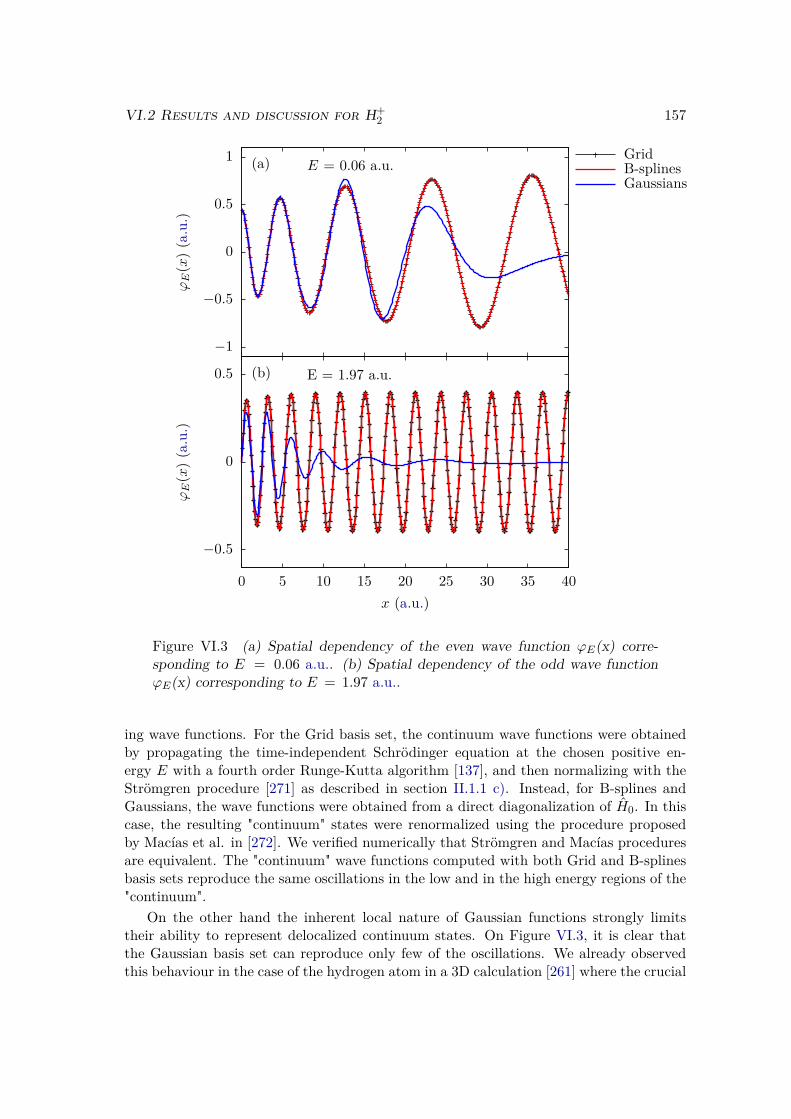
VI.2 Results and discussion for H+2 157
−1
−0.5
0
0.5
1 (a) E = 0.06 a.u.
−0.5
0
0.5
0 5 10 15 20 25 30 35 40
(b) E = 1.97 a.u.
ϕE
(x)(a.u.)
GridB-splinesGaussiansϕE
(x)(a.u.)
x (a.u.)
Figure VI.3 (a) Spatial dependency of the even wave function ϕE(x) corre-sponding to E = 0.06 a.u.. (b) Spatial dependency of the odd wave functionϕE(x) corresponding to E = 1.97 a.u..
ing wave functions. For the Grid basis set, the continuum wave functions were obtainedby propagating the time-independent Schrödinger equation at the chosen positive en-ergy E with a fourth order Runge-Kutta algorithm [137], and then normalizing with theStrömgren procedure [271] as described in section II.1.1 c). Instead, for B-splines andGaussians, the wave functions were obtained from a direct diagonalization of H0. In thiscase, the resulting "continuum" states were renormalized using the procedure proposedby Macías et al. in [272]. We verified numerically that Strömgren and Macías proceduresare equivalent. The "continuum" wave functions computed with both Grid and B-splinesbasis sets reproduce the same oscillations in the low and in the high energy regions of the"continuum".
On the other hand the inherent local nature of Gaussian functions strongly limitstheir ability to represent delocalized continuum states. On Figure VI.3, it is clear thatthe Gaussian basis set can reproduce only few of the oscillations. We already observedthis behaviour in the case of the hydrogen atom in a 3D calculation [261] where the crucial
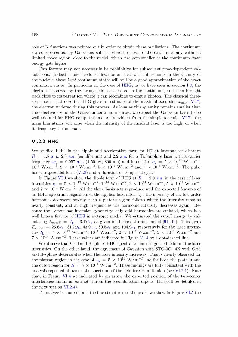
158 Chapter VI. Time-Dependent Configuration Interaction
role of K functions was pointed out in order to obtain these oscillations. The continuumstates represented by Gaussians will therefore be close to the exact one only within alimited space region, close to the nuclei, which size gets smaller as the continuum stateenergy gets higher.
This feature may not necessarily be prohibitive for subsequent time-dependent cal-culations. Indeed if one needs to describe an electron that remains in the vicinity ofthe nucleus, these local continuum states will still be a good approximation of the exactcontinuum states. In particular in the case of HHG, as we have seen in section I.3, theelectron is ionized by the strong field, accelerated in the continuum, and then broughtback close to its parent ion where it can recombine to emit a photon. The classical three-step model that describe HHG gives an estimate of the maximal excursion xmax (VI.7)the electron undergo during this process. As long as this quantity remains smaller thanthe effective size of the Gaussian continuum states, we expect the Gaussian basis to bewell adapted for HHG computations. As is evident from the simple formula (VI.7), themain limitations will arise when the intensity of the incident laser is too high, or whenits frequency is too small.
VI.2.2 HHG
We studied HHG in the dipole and acceleration form for H+2 at internuclear distance
R = 1.8 a.u., 2.0 a.u. (equilibrium) and 2.2 a.u. for a Ti:Sapphire laser with a carrierfrequency ωL = 0.057 a.u. (1.55 eV, 800 nm) and intensities IL = 5 × 10¹³ W.cm−2,1014 W.cm−2, 2 × 10¹⁴ W.cm−2, 5 × 10¹⁴ W.cm−2 and 7 × 10¹⁴ W.cm−2. The pulsehas a trapezoidal form (VI.8) and a duration of 10 optical cycles.
In Figure VI.4 we show the dipole form of HHG at R = 2.0 a.u. in the case of laserintensities IL = 5 × 10¹³ W.cm−2, 1014 W.cm−2, 2 × 10¹⁴ W.cm−2, 5 × 10¹⁴ W.cm−2
and 7 × 10¹⁴ W.cm−2. All the three basis sets reproduce well the expected features ofan HHG spectrum, regardless of the applied field intensity: the intensity of the low-orderharmonics decreases rapidly, then a plateau region follows where the intensity remainsnearly constant, and at high frequencies the harmonic intensity decreases again. Be-cause the system has inversion symmetry, only odd harmonics are emitted, which is awell known feature of HHG in isotropic media. We estimated the cutoff energy by cal-culating Ecutoff = Ip + 3.17Up as given in the rescattering model [91, 11]. This givesEcutoff = 25.6ωL, 31.7ωL, 43.9ωL, 80.5ωL and 104.9ωL respectively for the laser intensi-ties IL = 5 × 10¹³ W.cm−2, 1014 W.cm−2, 2 × 10¹⁴ W.cm−2, 5 × 10¹⁴ W.cm−2 and7 × 1014 W.cm−2. These values are indicated in Figure VI.4 by a dot-dashed line.
We observe that Grid and B-splines HHG spectra are indistinguishable for all the laserintensities. On the other hand, the agreement of Gaussian with STO-3G+4K with Gridand B-splines deteriorates when the laser intensity increases. This is clearly observed forthe plateau region in the case of IL = 5 × 10¹⁴ W.cm−2 and for both the plateau andthe cutoff region for IL = 7 × 10¹⁴ W.cm−2. These findings are fully consistent with theanalysis reported above on the spectrum of the field free Hamiltonian (see VI.2.1). Notethat, in Figure VI.4 we indicated by an arrow the expected position of the two-centerinterference minimum extracted from the recombination dipole. This will be detailed inthe next section VI.2.4).
To analyze in more details the fine structures of the peaks we show in Figure VI.5 the
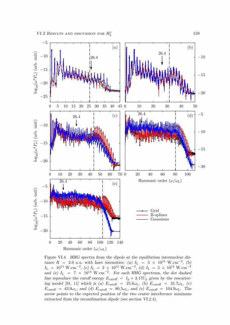
VI.2 Results and discussion for H+2 159
−25
−20
−15
−10
−5
0 5 10 15 20 25 30 35 40 45
(a)
26.4
0 10 20 30 40 50
−20
−15
−10
(b)26.4
−20
−15
−10
0 10 20 30 40 50 60 70
(c)26.4
0 20 40 60 80 100
−20
−15
−10
−5(d)26.4
−20
−15
−10
−5
0 20 40 60 80 100 120 140
(e)26.4
log 1
0(ω
4 Px)(a
rb.
unit)
log 1
0(ω
4 Px)(a
rb.
unit)
Harmonic order (ω/ωL)
log 1
0(ω
4 Px)(a
rb.
unit)
Harmonic order (ω/ωL)
GridB-splinesGaussians
Figure VI.4 HHG spectra from the dipole at the equilibrium internuclear dis-tance R = 2.0 a.u. with laser intensities: (a) IL = 5 × 10¹³ W.cm−2, (b)IL = 1014 W.cm−2, (c) IL = 2 × 10¹⁴ W.cm−2, (d) IL = 5 × 10¹⁴ W.cm−2
and (e) IL = 7 × 10¹⁴ W.cm−2. For each HHG spectrum, the dot dashedline reproduce the cutoff energy Ecutoff = Ip + 3.17Up given by the rescatter-ing model [91, 11] which is (a) Ecutoff = 25.6ωL, (b) Ecutoff = 31.7ωL, (c)Ecutoff = 43.9ωL, and (d) Ecutoff = 80.5ωL, and (e) Ecutoff = 104.9ωL. Thearrow points to the expected position of the two center interference minimumextracted from the recombination dipole (see section VI.2.4).

160 Chapter VI. Time-Dependent Configuration Interaction
−20
−18
−16
−14
−12
−10
−8
−6 (a)
−16
−14
−12
−10
−8(b)
−14
−12
−10
−8
−6
0 2 4 6 8 10 12 14 16
(c)
log 1
0(ω
4 Px)(a
rb.
unit)
log 1
0(ω
4 Px)(a
rb.
unit)
GridB-splinesGaussians
log 1
0(ω
4 Px)(a
rb.
unit)
Harmonic order (ω/ωL)
Figure VI.5 HHG spectra from the dipole at the equilibrium internuclear dis-tance R = 2.0 a.u. up to the 15th harmonic with laser intensities: (a)IL = 1014 W.cm−2, (b) IL = 2 × 10¹⁴ W.cm−2, and (c) IL = 5 × 10¹⁴ W.cm−2.The dashed line indicates the position of the harmonics while the dotted lineindicates the resonances due to the first excited state of H+
2 .
VI.2 Results and discussion for H+2 161
−24
−20
−16
−12
−8
−4(a)26.4
−24
−20
−16
−12
−8
(c)26.4
−24
−20
−16
−12
−8
0 20 40 60 80 100 120
(c)26.4
log 1
0Po
werspectrum
(arb.
unit)
Grid: dipleGrid: acceleration
log 1
0Po
werspectrum
(arb.
unit)
B-splines: dipoleB-splines: acceleration
log 1
0Po
werspectrum
(arb.
unit)
Harmonic order (ω/ωL)
Gaussians: dipoleGaussians: acceleration
Figure VI.6 HHG spectra in the dipole and acceleration form at the equilibriuminternuclear distance R = 2.0 a.u. with laser intensity IL = 5 × 10¹⁴ W.cm−2
calculated using (a) Grid, (b) B-splines and (c) Gaussians basis sets. The dash-dotted line is the cutoff energy Ecutoff = 80.5ωL. The arrow points to theexpected position of the two center interference minimum extracted from therecombination dipole which is identical to the one extracted from the recombi-nation acceleration (see section VI.2.4).
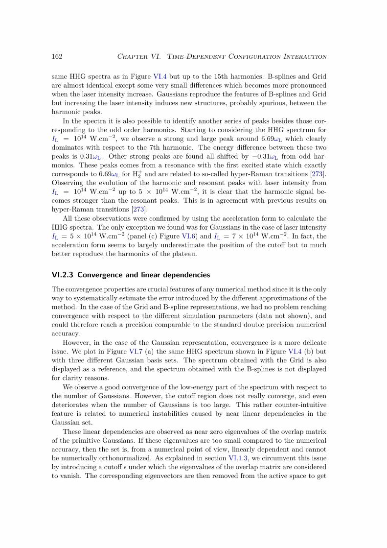
162 Chapter VI. Time-Dependent Configuration Interaction
same HHG spectra as in Figure VI.4 but up to the 15th harmonics. B-splines and Gridare almost identical except some very small differences which becomes more pronouncedwhen the laser intensity increase. Gaussians reproduce the features of B-splines and Gridbut increasing the laser intensity induces new structures, probably spurious, between theharmonic peaks.
In the spectra it is also possible to identify another series of peaks besides those cor-responding to the odd order harmonics. Starting to considering the HHG spectrum forIL = 1014 W.cm−2, we observe a strong and large peak around 6.69ωL which clearlydominates with respect to the 7th harmonic. The energy difference between these twopeaks is 0.31ωL. Other strong peaks are found all shifted by −0.31ωL from odd har-monics. These peaks comes from a resonance with the first excited state which exactlycorresponds to 6.69ωL for H+
2 and are related to so-called hyper-Raman transitions [273].Observing the evolution of the harmonic and resonant peaks with laser intensity fromIL = 1014 W.cm−2 up to 5 × 10¹⁴ W.cm−2, it is clear that the harmonic signal be-comes stronger than the resonant peaks. This is in agreement with previous results onhyper-Raman transitions [273].
All these observations were confirmed by using the acceleration form to calculate theHHG spectra. The only exception we found was for Gaussians in the case of laser intensityIL = 5 × 10¹⁴ W.cm−2 (panel (c) Figure VI.6) and IL = 7 × 10¹⁴ W.cm−2. In fact, theacceleration form seems to largely underestimate the position of the cutoff but to muchbetter reproduce the harmonics of the plateau.
VI.2.3 Convergence and linear dependencies
The convergence properties are crucial features of any numerical method since it is the onlyway to systematically estimate the error introduced by the different approximations of themethod. In the case of the Grid and B-spline representations, we had no problem reachingconvergence with respect to the different simulation parameters (data not shown), andcould therefore reach a precision comparable to the standard double precision numericalaccuracy.
However, in the case of the Gaussian representation, convergence is a more delicateissue. We plot in Figure VI.7 (a) the same HHG spectrum shown in Figure VI.4 (b) butwith three different Gaussian basis sets. The spectrum obtained with the Grid is alsodisplayed as a reference, and the spectrum obtained with the B-splines is not displayedfor clarity reasons.
We observe a good convergence of the low-energy part of the spectrum with respect tothe number of Gaussians. However, the cutoff region does not really converge, and evendeteriorates when the number of Gaussians is too large. This rather counter-intuitivefeature is related to numerical instabilities caused by near linear dependencies in theGaussian set.
These linear dependencies are observed as near zero eigenvalues of the overlap matrixof the primitive Gaussians. If these eigenvalues are too small compared to the numericalaccuracy, then the set is, from a numerical point of view, linearly dependent and cannotbe numerically orthonormalized. As explained in section VI.1.3, we circumvent this issueby introducing a cutoff ε under which the eigenvalues of the overlap matrix are consideredto vanish. The corresponding eigenvectors are then removed from the active space to get
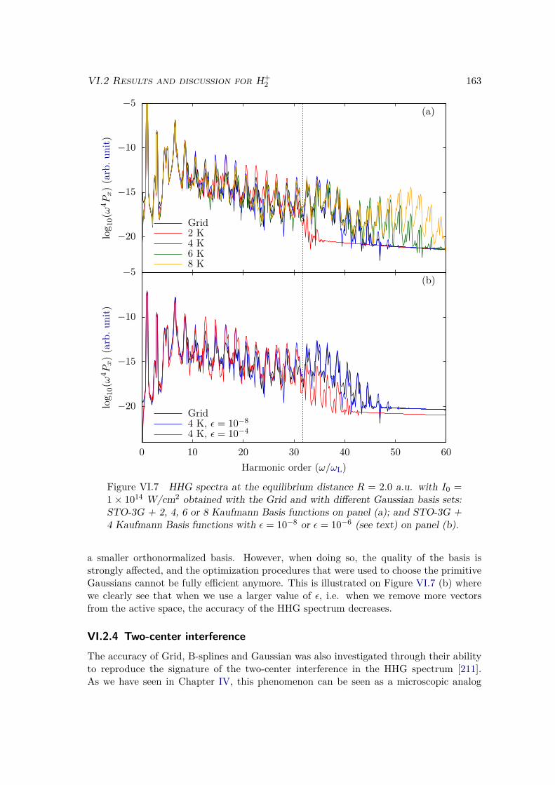
VI.2 Results and discussion for H+2 163
−20
−15
−10
−5(a)
−20
−15
−10
−5
0 10 20 30 40 50 60
(b)
log 1
0(ω
4 Px)(a
rb.
unit)
Grid2 K4 K6 K8 K
log 1
0(ω
4 Px)(a
rb.
unit)
Harmonic order (ω/ωL)
Grid4 K, ε = 10−8
4 K, ε = 10−4
Figure VI.7 HHG spectra at the equilibrium distance R = 2.0 a.u. with I0 =1× 10¹⁴ W/cm2 obtained with the Grid and with different Gaussian basis sets:STO-3G + 2, 4, 6 or 8 Kaufmann Basis functions on panel (a); and STO-3G +4 Kaufmann Basis functions with ε = 10−8 or ε = 10−6 (see text) on panel (b).
a smaller orthonormalized basis. However, when doing so, the quality of the basis isstrongly affected, and the optimization procedures that were used to choose the primitiveGaussians cannot be fully efficient anymore. This is illustrated on Figure VI.7 (b) wherewe clearly see that when we use a larger value of ε, i.e. when we remove more vectorsfrom the active space, the accuracy of the HHG spectrum decreases.
VI.2.4 Two-center interference
The accuracy of Grid, B-splines and Gaussian was also investigated through their abilityto reproduce the signature of the two-center interference in the HHG spectrum [211].As we have seen in Chapter IV, this phenomenon can be seen as a microscopic analog
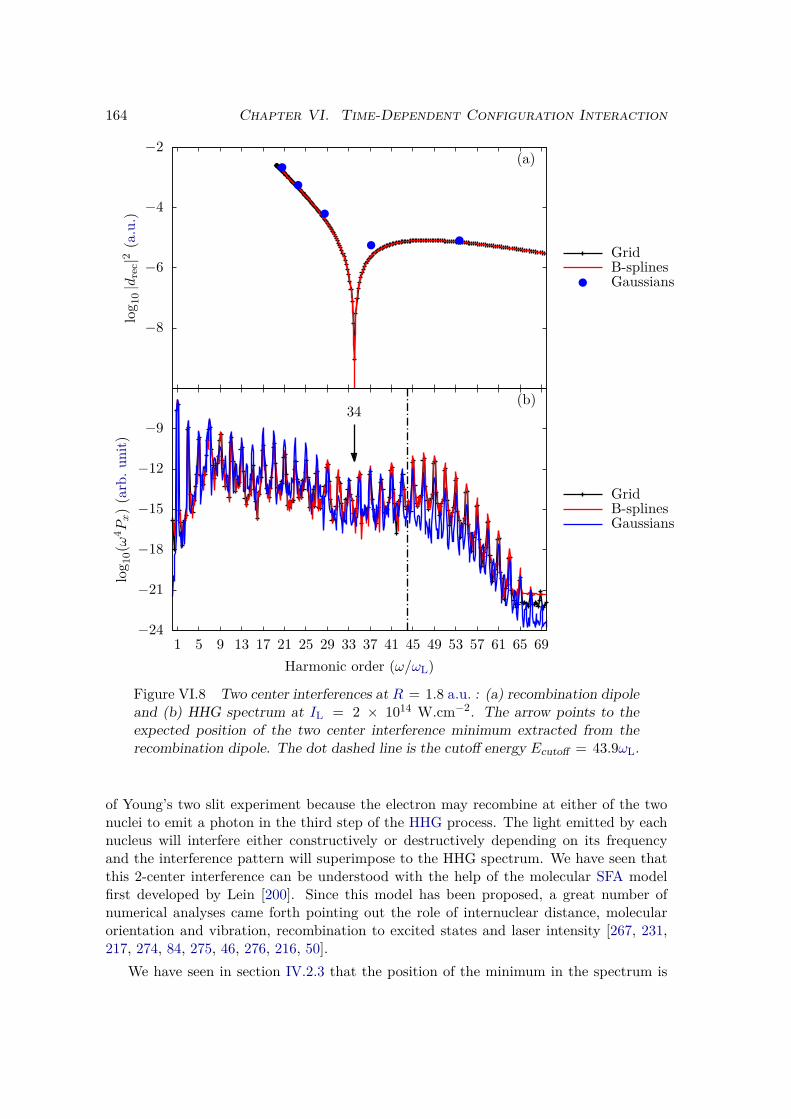
164 Chapter VI. Time-Dependent Configuration Interaction
−8
−6
−4
−2(a)
−24
−21
−18
−15
−12
−9
1 5 9 13 17 21 25 29 33 37 41 45 49 53 57 61 65 69
(b)34
log 1
0|d
rec|2
(a.u.)
GridB-splinesGaussians
log 1
0(ω
4 Px)(a
rb.
unit)
Harmonic order (ω/ωL)
GridB-splinesGaussians
Figure VI.8 Two center interferences at R = 1.8 a.u. : (a) recombination dipoleand (b) HHG spectrum at IL = 2 × 10¹⁴ W.cm−2. The arrow points to theexpected position of the two center interference minimum extracted from therecombination dipole. The dot dashed line is the cutoff energy Ecutoff = 43.9ωL.
of Young’s two slit experiment because the electron may recombine at either of the twonuclei to emit a photon in the third step of the HHG process. The light emitted by eachnucleus will interfere either constructively or destructively depending on its frequencyand the interference pattern will superimpose to the HHG spectrum. We have seen thatthis 2-center interference can be understood with the help of the molecular SFA modelfirst developed by Lein [200]. Since this model has been proposed, a great number ofnumerical analyses came forth pointing out the role of internuclear distance, molecularorientation and vibration, recombination to excited states and laser intensity [267, 231,217, 274, 84, 275, 46, 276, 216, 50].
We have seen in section IV.2.3 that the position of the minimum in the spectrum is
VI.2 Results and discussion for H+2 165
−8
−6
−4
−2(a)
−24
−21
−18
−15
−12
−9
1 5 9 13 17 21 25 29 33 37 41 45 49 53 57 61 65 69
(b)26.4
log 1
0|d
rec|2
(a.u.)
GridB-splinesGaussians
log 1
0(ω
4 Px)(a
rb.
unit)
Harmonic order (ω/ωL)
GridB-splinesGaussians
Figure VI.9 Two center interferences at R = 2.0 a.u. : (a) recombination dipoleand (b) HHG spectrum at IL = 2 × 10¹⁴ W.cm−2. The arrow points to theexpected position of the two center interference minimum extracted from therecombination dipole. The dot dashed line is the cutoff energy Ecutoff = 43.9ωL.
independent on the laser intensity and can be extracted from the analysis of the recom-bination dipole drec(E) = 〈ϕ0|x|ϕE〉 [211] where ϕ0 is the ground state and ϕE is acontinuum state at energy E of H0. This quantity is plotted in panel (a) of Figure VI.8for R = 1.8 a.u., in panel (a) of Figure VI.9 for R = 2.0 a.u. and in panel (a) ofFigure VI.10 for R = 2.2 a.u.. We observe that, as in section IV.2.3, the position of theminimum in the HHG spectrum is well predicted by the first zero of the recombinationdipole in the considered energy range. We found that this corresponds to ωmin = 34.0ωLfor R = 1.8 a.u., 26.4ωL for R = 2.0 a.u. and 20.8ωL for R = 2.2 a.u.. We would liketo note that the extraction of the minimum from the recombination dipole is straightfor-ward for Grid and B-splines, while in the case of Gaussians the density of "continuum"
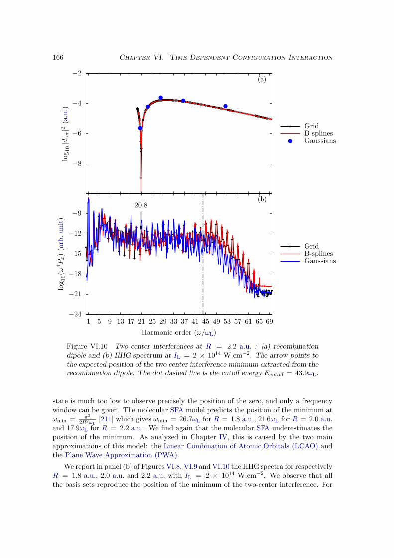
166 Chapter VI. Time-Dependent Configuration Interaction
−8
−6
−4
−2(a)
−24
−21
−18
−15
−12
−9
1 5 9 13 17 21 25 29 33 37 41 45 49 53 57 61 65 69
(b)20.8
log 1
0|d
rec|2
(a.u.)
GridB-splinesGaussians
log 1
0(ω
4 Px)(a
rb.
unit)
Harmonic order (ω/ωL)
GridB-splinesGaussians
Figure VI.10 Two center interferences at R = 2.2 a.u. : (a) recombinationdipole and (b) HHG spectrum at IL = 2 × 10¹⁴ W.cm−2. The arrow points tothe expected position of the two center interference minimum extracted from therecombination dipole. The dot dashed line is the cutoff energy Ecutoff = 43.9ωL.
state is much too low to observe precisely the position of the zero, and only a frequencywindow can be given. The molecular SFA model predicts the position of the minimum atωmin = π2
2R2ωL[211] which gives ωmin = 26.7ωL for R = 1.8 a.u., 21.6ωL for R = 2.0 a.u.
and 17.9ωL for R = 2.2 a.u.. We find again that the molecular SFA underestimates theposition of the minimum. As analyzed in Chapter IV, this is caused by the two mainapproximations of this model: the Linear Combination of Atomic Orbitals (LCAO) andthe Plane Wave Approximation (PWA).
We report in panel (b) of Figures VI.8, VI.9 and VI.10 the HHG spectra for respectivelyR = 1.8 a.u., 2.0 a.u. and 2.2 a.u. with IL = 2 × 10¹⁴ W.cm−2. We observe that allthe basis sets reproduce the position of the minimum of the two-center interference. For
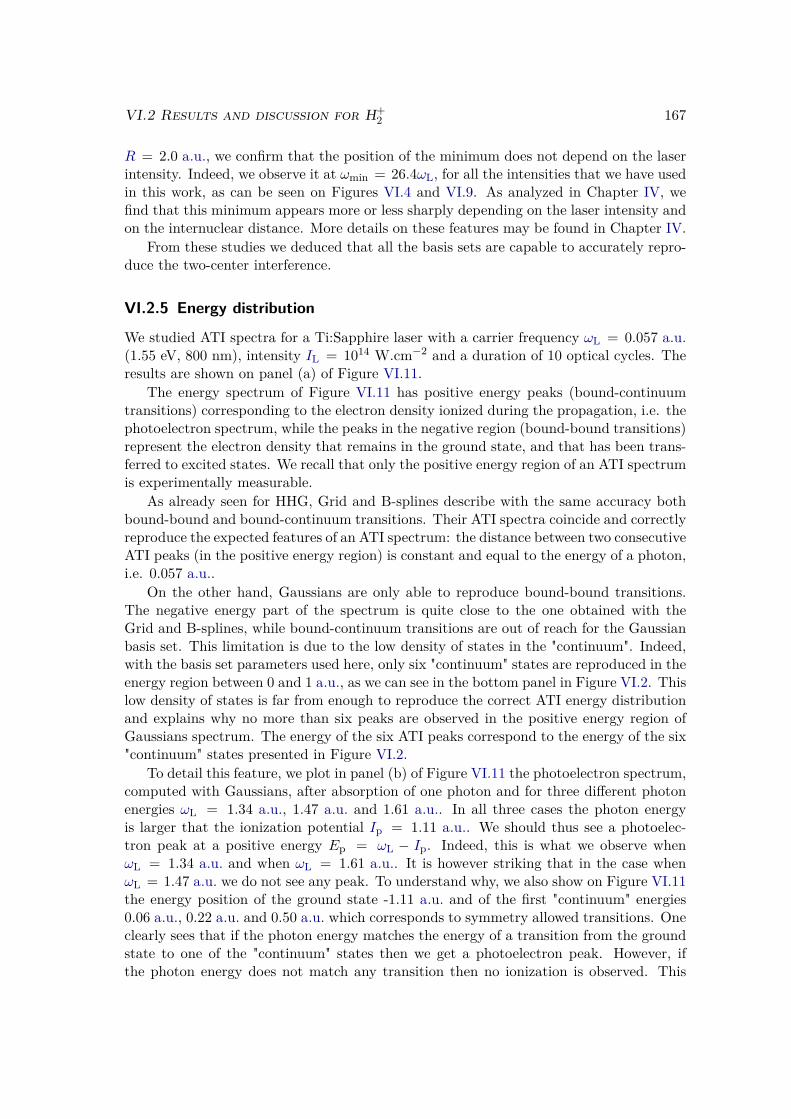
VI.2 Results and discussion for H+2 167
R = 2.0 a.u., we confirm that the position of the minimum does not depend on the laserintensity. Indeed, we observe it at ωmin = 26.4ωL, for all the intensities that we have usedin this work, as can be seen on Figures VI.4 and VI.9. As analyzed in Chapter IV, wefind that this minimum appears more or less sharply depending on the laser intensity andon the internuclear distance. More details on these features may be found in Chapter IV.
From these studies we deduced that all the basis sets are capable to accurately repro-duce the two-center interference.
VI.2.5 Energy distribution
We studied ATI spectra for a Ti:Sapphire laser with a carrier frequency ωL = 0.057 a.u.(1.55 eV, 800 nm), intensity IL = 1014 W.cm−2 and a duration of 10 optical cycles. Theresults are shown on panel (a) of Figure VI.11.
The energy spectrum of Figure VI.11 has positive energy peaks (bound-continuumtransitions) corresponding to the electron density ionized during the propagation, i.e. thephotoelectron spectrum, while the peaks in the negative region (bound-bound transitions)represent the electron density that remains in the ground state, and that has been trans-ferred to excited states. We recall that only the positive energy region of an ATI spectrumis experimentally measurable.
As already seen for HHG, Grid and B-splines describe with the same accuracy bothbound-bound and bound-continuum transitions. Their ATI spectra coincide and correctlyreproduce the expected features of an ATI spectrum: the distance between two consecutiveATI peaks (in the positive energy region) is constant and equal to the energy of a photon,i.e. 0.057 a.u..
On the other hand, Gaussians are only able to reproduce bound-bound transitions.The negative energy part of the spectrum is quite close to the one obtained with theGrid and B-splines, while bound-continuum transitions are out of reach for the Gaussianbasis set. This limitation is due to the low density of states in the "continuum". Indeed,with the basis set parameters used here, only six "continuum" states are reproduced in theenergy region between 0 and 1 a.u., as we can see in the bottom panel in Figure VI.2. Thislow density of states is far from enough to reproduce the correct ATI energy distributionand explains why no more than six peaks are observed in the positive energy region ofGaussians spectrum. The energy of the six ATI peaks correspond to the energy of the six"continuum" states presented in Figure VI.2.
To detail this feature, we plot in panel (b) of Figure VI.11 the photoelectron spectrum,computed with Gaussians, after absorption of one photon and for three different photonenergies ωL = 1.34 a.u., 1.47 a.u. and 1.61 a.u.. In all three cases the photon energyis larger that the ionization potential Ip = 1.11 a.u.. We should thus see a photoelec-tron peak at a positive energy Ep = ωL − Ip. Indeed, this is what we observe whenωL = 1.34 a.u. and when ωL = 1.61 a.u.. It is however striking that in the case whenωL = 1.47 a.u. we do not see any peak. To understand why, we also show on Figure VI.11the energy position of the ground state -1.11 a.u. and of the first "continuum" energies0.06 a.u., 0.22 a.u. and 0.50 a.u. which corresponds to symmetry allowed transitions. Oneclearly sees that if the photon energy matches the energy of a transition from the groundstate to one of the "continuum" states then we get a photoelectron peak. However, ifthe photon energy does not match any transition then no ionization is observed. This
168 Chapter VI. Time-Dependent Configuration Interaction
−12
−10
−8
−6
−4
−2
0(a)
−14
−12
−10
−8
−6
−4
−2
−1 −0.5 0 0.5
(b)
photon energiesstate energies
log 1
0Ene
rgyspectrum
(arb.
unit)
GridB-splinesGaussians
log 1
0Ene
rgyspectrum
(arb.
unit)
E (a.u.)
Figure VI.11 (a) ATI spectrum calculated at the equilibrium interatomic dis-tance R = 2.0 a.u.. (b) Photoelectron spectrum computed with the Gaussianbasis set at the equilibrium distance R = 2.0 a.u. with IL = 1014 W.cm−2
and ωL = 1.34 a.u. (black), ωL = 1.47 a.u. (red) and ωL = 1.61 a.u. (blue).The ground state energy (-1.11 a.u.) and the continuum energy states (0.06 a.u.,0.22 a.u. and 0.50 a.u.) which corresponds to transitions allowed by symmetryare displayed (magenta dots).
crucial feature forbids the computation of a correct photoelectron or ATI spectrum withthe Gaussians basis set used here. We believe that larger basis sets can in principle de-scribe ATI, however linear dependencies of Gaussians can limit their applicability for suchnon-linear processes.
VI.3 One dimensional bielectronic models 169
VI.3 One dimensional bielectronic models
We now generalize the use of the Grid and Gaussian basis sets to multi-electron species.In this section we consider bielectronic model systems, with one dimension for each elec-tron. The advantage of such systems is that we can perform accurate simulations onbidimensional grid, and thus have a deep comparison of the methods.
We define a one dimensional bielectronic model for H2 with the field-free Hamiltonian:
H0 = −12∂2
∂x21− 1
2∂2
∂x22
+ V0(x1) + V0(x2) + Vee(x1, x2), (VI.10)
where the nuclei-electron interaction potential V0 is a one dimensional molecular Soft-Coulomb potential (II.2) with regularization parameter aH2 , and where the interelectronicrepulsion Vee is a Soft-Coulomb potential (II.1) with regularization parameter bH2 . Theparameters aH2 and bH2 are chosen to reproduce the ground state energy and verticalionization potential of H2 at a given internuclear distance. We did the simulations at theequilibrium distance R = 1.408 a.u., with aH2 = 1.991 a.u. and bH2 = 5.345 a.u., whichreproduces E0 = −1.384 a.u. and Ip = 0.604 a.u..
For comparison purposes we also investigated a one dimensional bielectronic modelfor the Helium atom. In this case the regularization parameter are aHe = 0.707 a.u. andbHe = 0.582 a.u., which reproduces E0 = −1.91 a.u. and Ip = 0.91 a.u..
We chose exactly the same laser parameters as for the 1D simulations of H+2 (see
section VI.1.4).
VI.3.1 Real-space bidimensional grid
As described in section II.2.1, the time-dependent wave function is discretized on a real-space bidimensional square grid of N × N points (xi, yj). It is thus represented by thevector
|ψ(t)〉 ≡ (ψ(x1, y1, t), . . . , ψ(xi, yj , t), . . . , ψ(xN , yN , t)). (VI.11)
The TDSE is solved by means of the split-operator algorithm (see section II.2.2). TheH+
2 ground state computed by imaginary time propagation (see section II.2.3) is takenas the initial state in the propagation. In addition, to avoid unphysical reflections at theboundaries of the simulation grid, a mask-type absorber function [143] was implementedwith a spatial extension of habs = 100 a.u. (see section II.1.1 c)) at each boundary of the2D box.
VI.3.2 Gaussian-based TDCI
The time-dependent wave function is expanded on the basis of the eigenvectors of thefield-free Hamiltonian H0:
ψ(x1, x2, t) =∑i
ci(t)ϕi(x1, x2). (VI.12)
These eigenvectors are themselves computed with a Gaussian-based Configuration Inter-action (CI) algorithm [270]. They are expressed in the basis of the two electron spin
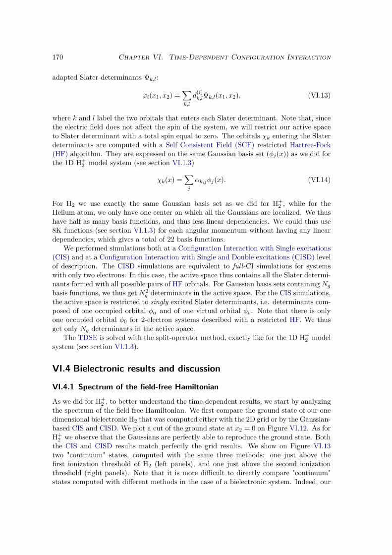
170 Chapter VI. Time-Dependent Configuration Interaction
adapted Slater determinants Ψk,l:
ϕi(x1, x2) =∑k,l
d(i)k,lΨk,l(x1, x2), (VI.13)
where k and l label the two orbitals that enters each Slater determinant. Note that, sincethe electric field does not affect the spin of the system, we will restrict our active spaceto Slater determinant with a total spin equal to zero. The orbitals χk entering the Slaterdeterminants are computed with a Self Consistent Field (SCF) restricted Hartree-Fock(HF) algorithm. They are expressed on the same Gaussian basis set (φj(x)) as we did forthe 1D H+
2 model system (see section VI.1.3)
χk(x) =∑j
αk,jφj(x). (VI.14)
For H2 we use exactly the same Gaussian basis set as we did for H+2 , while for the
Helium atom, we only have one center on which all the Gaussians are localized. We thushave half as many basis functions, and thus less linear dependencies. We could thus use8K functions (see section VI.1.3) for each angular momentum without having any lineardependencies, which gives a total of 22 basis functions.
We performed simulations both at a Configuration Interaction with Single excitations(CIS) and at a Configuration Interaction with Single and Double excitations (CISD) levelof description. The CISD simulations are equivalent to full-CI simulations for systemswith only two electrons. In this case, the active space thus contains all the Slater determi-nants formed with all possible pairs of HF orbitals. For Gaussian basis sets containing Ng
basis functions, we thus get N2g determinants in the active space. For the CIS simulations,
the active space is restricted to singly excited Slater determinants, i.e. determinants com-posed of one occupied orbital φα and of one virtual orbital φv. Note that there is onlyone occupied orbital φ0 for 2-electron systems described with a restricted HF. We thusget only Ng determinants in the active space.
The TDSE is solved with the split-operator method, exactly like for the 1D H+2 model
system (see section VI.1.3).
VI.4 Bielectronic results and discussion
VI.4.1 Spectrum of the field-free Hamiltonian
As we did for H+2 , to better understand the time-dependent results, we start by analyzing
the spectrum of the field free Hamiltonian. We first compare the ground state of our onedimensional bielectronic H2 that was computed either with the 2D grid or by the Gaussian-based CIS and CISD. We plot a cut of the ground state at x2 = 0 on Figure VI.12. As forH+
2 we observe that the Gaussians are perfectly able to reproduce the ground state. Boththe CIS and CISD results match perfectly the grid results. We show on Figure VI.13two "continuum" states, computed with the same three methods: one just above thefirst ionization threshold of H2 (left panels), and one just above the second ionizationthreshold (right panels). Note that it is more difficult to directly compare "continuum"states computed with different methods in the case of a bielectronic system. Indeed, our
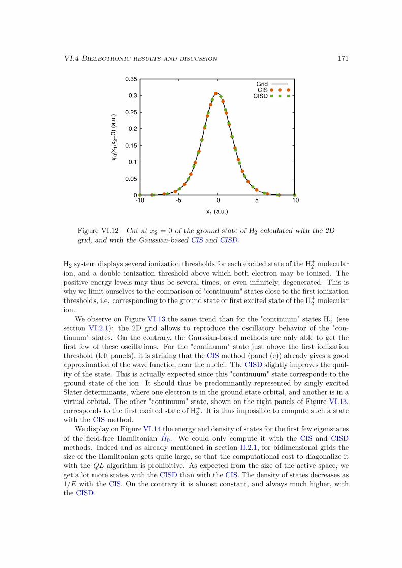
VI.4 Bielectronic results and discussion 171
0
0.05
0.1
0.15
0.2
0.25
0.3
0.35
-10 -5 0 5 10
ϕ0(
x 1,x
2=0)
(a.u
.)
x1 (a.u.)
GridCIS
CISD
Figure VI.12 Cut at x2 = 0 of the ground state of H2 calculated with the 2Dgrid, and with the Gaussian-based CIS and CISD.
H2 system displays several ionization thresholds for each excited state of the H+2 molecular
ion, and a double ionization threshold above which both electron may be ionized. Thepositive energy levels may thus be several times, or even infinitely, degenerated. This iswhy we limit ourselves to the comparison of "continuum" states close to the first ionizationthresholds, i.e. corresponding to the ground state or first excited state of the H+
2 molecularion.
We observe on Figure VI.13 the same trend than for the "continuum" states H+2 (see
section VI.2.1): the 2D grid allows to reproduce the oscillatory behavior of the "con-tinuum" states. On the contrary, the Gaussian-based methods are only able to get thefirst few of these oscillations. For the "continuum" state just above the first ionizationthreshold (left panels), it is striking that the CIS method (panel (e)) already gives a goodapproximation of the wave function near the nuclei. The CISD slightly improves the qual-ity of the state. This is actually expected since this "continuum" state corresponds to theground state of the ion. It should thus be predominantly represented by singly excitedSlater determinants, where one electron is in the ground state orbital, and another is in avirtual orbital. The other "continuum" state, shown on the right panels of Figure VI.13,corresponds to the first excited state of H+
2 . It is thus impossible to compute such a statewith the CIS method.
We display on Figure VI.14 the energy and density of states for the first few eigenstatesof the field-free Hamiltonian H0. We could only compute it with the CIS and CISDmethods. Indeed and as already mentioned in section II.2.1, for bidimensional grids thesize of the Hamiltonian gets quite large, so that the computational cost to diagonalize itwith the QL algorithm is prohibitive. As expected from the size of the active space, weget a lot more states with the CISD than with the CIS. The density of states decreases as1/E with the CIS. On the contrary it is almost constant, and always much higher, withthe CISD.
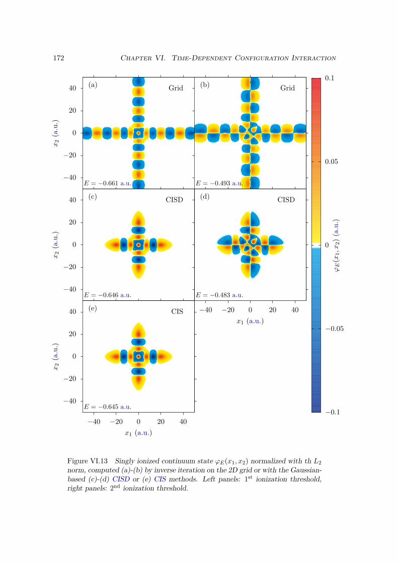
172 Chapter VI. Time-Dependent Configuration Interaction
−40
−20
0
20
40
−40
−20
0
20
40
−40 −20 0 20 40
−40
−20
0
20
40
−40 −20 0 20 40
x2(a.u.)
(a) Grid
E = −0.661 a.u.
(b) Grid
E = −0.493 a.u.
x2(a.u.)
(c) CISD
E = −0.646 a.u.
x1 (a.u.)
(d) CISD
E = −0.483 a.u.
x2(a.u.)
x1 (a.u.)
−0.1
−0.05
0
0.05
0.1
ϕE
(x1,x
2)(a.u.)
(e) CIS
E = −0.645 a.u.
Figure VI.13 Singly ionized continuum state ϕE(x1, x2) normalized with th L2norm, computed (a)-(b) by inverse iteration on the 2D grid or with the Gaussian-based (c)-(d) CISD or (e) CIS methods. Left panels: 1st ionization threshold,right panels: 2nd ionization threshold.
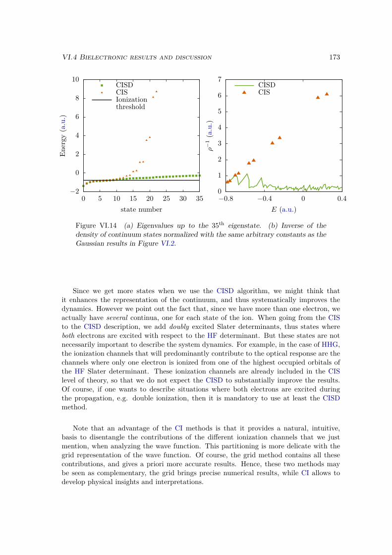
VI.4 Bielectronic results and discussion 173
−2
0
2
4
6
8
10
0 5 10 15 20 25 30 350
1
2
3
4
5
6
7
−0.8 −0.4 0 0.4
Energy
(a.u.)
state number
CISDCISIonizationthreshold
ρ−
1(a.u.)
E (a.u.)
CISDCIS
Figure VI.14 (a) Eigenvalues up to the 35th eigenstate. (b) Inverse of thedensity of continuum states normalized with the same arbitrary constants as theGaussian results in Figure VI.2.
Since we get more states when we use the CISD algorithm, we might think thatit enhances the representation of the continuum, and thus systematically improves thedynamics. However we point out the fact that, since we have more than one electron, weactually have several continua, one for each state of the ion. When going from the CISto the CISD description, we add doubly excited Slater determinants, thus states whereboth electrons are excited with respect to the HF determinant. But these states are notnecessarily important to describe the system dynamics. For example, in the case of HHG,the ionization channels that will predominantly contribute to the optical response are thechannels where only one electron is ionized from one of the highest occupied orbitals ofthe HF Slater determinant. These ionization channels are already included in the CISlevel of theory, so that we do not expect the CISD to substantially improve the results.Of course, if one wants to describe situations where both electrons are excited duringthe propagation, e.g. double ionization, then it is mandatory to use at least the CISDmethod.
Note that an advantage of the CI methods is that it provides a natural, intuitive,basis to disentangle the contributions of the different ionization channels that we justmention, when analyzing the wave function. This partitioning is more delicate with thegrid representation of the wave function. Of course, the grid method contains all thesecontributions, and gives a priori more accurate results. Hence, these two methods maybe seen as complementary, the grid brings precise numerical results, while CI allows todevelop physical insights and interpretations.
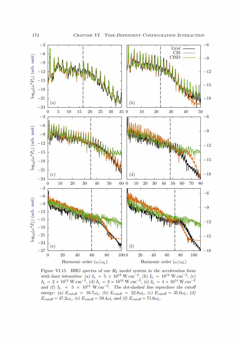
174 Chapter VI. Time-Dependent Configuration Interaction
−24
−21
−18
−15
−12
−9
−6
−3
0 5 10 15 20 25 30 35
(a)
0 10 20 30 40 50
−18
−15
−12
−9
−6
(b)
−24
−21
−18
−15
−12
−9
−6
−3
0 10 20 30 40 50 60
(c)
0 10 20 30 40 50 60 70 80
−18
−15
−12
−9
−6
(d)
−27−24−21−18−15−12−9−6−3
0 20 40 60 80 100
(e)
0 20 40 60 80 100−18
−15
−12
−9
−6
(f)
log 1
0(ω
4 Px)(a
rb.
unit)
GridCIS
CISD
log 1
0(ω
4 Px)(a
rb.
unit)
log 1
0(ω
4 Px)(a
rb.
unit)
Harmonic order (ω/ωL) Harmonic order (ω/ωL)
Figure VI.15 HHG spectra of our H2 model system in the acceleration formwith laser intensities: (a) IL = 5 × 10¹³ W.cm−2, (b) IL = 1014 W.cm−2, (c)IL = 2 × 10¹⁴ W.cm−2, (d) IL = 3 × 10¹⁴ W.cm−2, (e) IL = 4 × 10¹⁴ W.cm−2
and (f) IL = 5 × 10¹⁴ W.cm−2. The dot-dashed line reproduce the cutoffenergy: (a) Ecutoff = 16.7ωL, (b) Ecutoff = 22.8ωL, (c) Ecutoff = 35.0ωL, (d)Ecutoff = 47.2ωL, (e) Ecutoff = 59.4ωL and (f) Ecutoff = 71.6ωL.
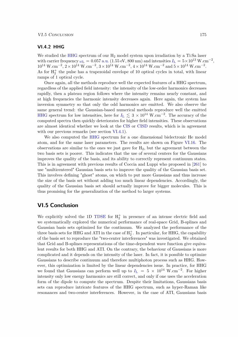
VI.5 Conclusion 175
VI.4.2 HHG
We studied the HHG spectrum of our H2 model system upon irradiation by a Ti:Sa laserwith carrier frequency ωL = 0.057 a.u. (1.55 eV, 800 nm) and intensities IL = 5×10¹³ W.cm−2,1014 W.cm−2, 2×10¹⁴ W.cm−2, 3×10¹⁴ W.cm−2, 4×10¹⁴ W.cm−2 and 5×10¹⁴ W.cm−2.As for H+
2 the pulse has a trapezoidal envelope of 10 optical cycles in total, with linearramps of 1 optical cycle.
Once again, all the methods reproduce well the expected features of a HHG spectrum,regardless of the applied field intensity: the intensity of the low-order harmonics decreasesrapidly, then a plateau region follows where the intensity remains nearly constant, andat high frequencies the harmonic intensity decreases again. Here again, the system hasinversion symmetry so that only the odd harmonics are emitted. We also observe thesame general trend: the Gaussian-based numerical methods reproduce well the emittedHHG spectrum for low intensities, here for IL . 3 × 10¹⁴ W.cm−2. The accuracy of thecomputed spectra then quickly deteriorates for higher field intensities. These observationsare almost identical whether we look at the CIS or CISD results, which is in agreementwith our previous remarks (see section VI.4.1).
We also computed the HHG spectrum for a one dimensional bielectronic He modelatom, and for the same laser parameters. The results are shown on Figure VI.16. Theobservations are similar to the ones we just gave for H2, but the agreement between thetwo basis sets is poorer. This indicates that the use of several centers for the Gaussiansimproves the quality of the basis, and its ability to correctly represent continuum states.This is in agreement with previous results of Coccia and Luppi who proposed in [261] touse "multicentered" Gaussian basis sets to improve the quality of the Gaussian basis set.This involves defining "ghost" atoms, on which to put more Gaussians and thus increasethe size of the basis set without adding too much linear dependencies. Accordingly, thequality of the Gaussian basis set should actually improve for bigger molecules. This isthus promising for the generalization of the method to larger systems.
VI.5 Conclusion
We explicitly solved the 1D TDSE for H+2 in presence of an intense electric field and
we systematically explored the numerical performance of real-space Grid, B-splines andGaussian basis sets optimized for the continuum. We analyzed the performance of thethree basis sets for HHG and ATI in the case of H+
2 . In particular, for HHG, the capabilityof the basis set to reproduce the "two-center interferences" was investigated. We obtainedthat Grid and B-splines representations of the time-dependent wave function give equiva-lent results for both HHG and ATI. On the contrary, the behaviour of Gaussians is morecomplicated and it depends on the intensity of the laser. In fact, it is possible to optimizeGaussians to describe continuum and therefore multiphoton process such as HHG. How-ever, this optimization is limited by the linear dependencies issue. In practice, for HHGwe found that Gaussians can perform well up to IL = 5 × 10¹⁴ W.cm−2. For higherintensity only low energy harmonics are still correct, and only if one uses the accelerationform of the dipole to compute the spectrum. Despite their limitations, Gaussians basissets can reproduce intricate features of the HHG spectrum, such as hyper-Raman likeresonances and two-center interferences. However, in the case of ATI, Gaussians basis
176 Chapter VI. Time-Dependent Configuration Interaction
−24
−21
−18
−15
−12
−9
−6
−3
0 5 10 15 20 25 30 35 40
(a)
0 10 20 30 40 50
−18
−15
−12
−9
−6
(b)
−21
−18
−15
−12
−9
−6
−3
0 10 20 30 40 50 60
(c)
0 10 20 30 40 50 60 70 80
−18
−15
−12
−9
−6
(d)
−24−21−18−15−12−9−6−3
0
0 20 40 60 80 100
(e)
0 20 40 60 80 100−18
−15
−12
−9
−6
(f)
log 1
0(ω
4 Px)(a
rb.
unit)
GridCIS
CISD
log 1
0(ω
4 Px)(a
rb.
unit)
log 1
0(ω
4 Px)(a
rb.
unit)
Harmonic order (ω/ωL) Harmonic order (ω/ωL)
Figure VI.16 HHG spectra of our Helium model system in the acceleration formwith laser intensities: (a) IL = 5 × 10¹³ W.cm−2, (b) IL = 1014 W.cm−2, (c)IL = 2 × 10¹⁴ W.cm−2, (d) IL = 3 × 10¹⁴ W.cm−2, (e) IL = 4 × 10¹⁴ W.cm−2
and (f) IL = 5 × 10¹⁴ W.cm−2. The dot-dashed line reproduce the cutoffenergy: (a) Ecutoff = 22.1ωL, (b) Ecutoff = 28.2ωL, (c) Ecutoff = 40.4ωL, (d)Ecutoff = 52.5ωL, (e) Ecutoff = 64.7ωL and (f) Ecutoff = 76.9ωL.
VI.5 Conclusion 177
sets cannot possibly describe a correct spectrum.We then assessed the accuracy of the TDCI method to reproduce the HHG spectra
of bielectronic model systems for H2 and for the Helium atom. We found that alreadyfor such small systems bidimensional grid are numerically demanding, while the TDCImethod remains very cheap, even at the CISD level of description. Moreover, we sawthat the Gaussian-based TDCI is actually able to reproduce correctly the HHG spec-trum of both bielectronic systems as long as the intensity is not too high, i.e. up toIL ∼ 5× 10¹³ W.cm−2 for our 1D Helium atom and up to IL ∼ 2 × 10¹⁴ W.cm−2 for our1D H2 molecule. For higher intensities only the low energy harmonics are reproduced.The Gaussian-based TDCI performed much better on the H2 molecule than it did forthe Helium atom. We strongly believe that it is related to the number of centers onwhich we place the Gaussians of the basis. Indeed, multicentered Gaussian basis sets arenumerically more efficient because they generate less linear dependencies. This featuregives promising perspectives for the description of larger molecules. Finally, we showedthat the double excitations contribute almost nothing to the HHG emission, so that theCIS level of description is sufficient. For systems with more than two electrons, this cansave a lot of computational resources, and would thus allow to generalize the method tolarger species very easily.

178 Chapter VI. Time-Dependent Configuration Interaction
Conclusion
During my PhD I studied different aspects of the interaction of atoms and molecules withstrong laser fields. I developed analytical models to understand the mechanisms at thebasis of the correlated and highly non-linear processes that are observed in strong fieldphysics. The strength of these approximate models lies in their ability to reach interpre-tations and insight on physical phenomena. To support my interpretations, I combinedthis approach with the results of accurate numerical simulations performed on toy modelsystems. These simple models actually present many advantages. On the one hand theyallow to tune all their fundamental parameters, and thus to concentrate on one of severalparticular physical issues. Moreover their low dimensionality enables to perform exten-sive numerical treatments. In particular I solved both the Time-Dependent SchrödingerEquation (TDSE) and the Time-Independent Schrödinger Equation (TISE) to extract asmany information as possible from the resulting time-dependent wave function. I alsoexploited these numerical simulations to meticulously test the underlying approximationsof the developed analytical models.
More precisely, I investigated the electronic and nuclear dynamics of atoms and di-atomic molecules in intense femtosecond laser pulses. I first concentrated on the highlynon-linear electronic processes that are triggered by such laser pulses, like ATI, HHG ornon sequential multiple ionization. In Chapter III, I studied the common first step of allthese processes, the archetype of the quantum effect with no classical equivalent whatso-ever, namely tunnel ionization. In an infrared laser field, the time variations of the electricfield are very slow with respect to the natural electronic time scales, so that the ionizationyield can be directly deduced from the time-independent problem in a static electric field.I studied this ionization yield for several atomic and molecular model systems. I showedthe importance of the DC Stark shift, both for quantitative and qualitative descriptionsof tunnel ionization, and I derived an analytical expression in the semi-classical approxi-mation that takes this effect into account. I showed that the Stark shift is the dominantcontribution to the anisotropy of the tunnel emission in asymmetric molecules. I demon-strated how crucial the accurate calculation of this Stark shift can be, especially for highlypolarizable molecules for which second order perturbation theory breaks down. What ismore, I analyzed the reasons that causes discrepancies between the asymptotic analyticalformula and the numerically exact simulations. I could disentangle the error induced bythe different approximations used in the asymptotic derivation, and I found that some ofthese approximations are actually severally unjustified at working laser intensities, butthat, thanks to a fortunate error compensation, the final results were still reasonable.
One of the direct applications of strong field physics is High order Harmonic generationSpectroscopy (HHS), where the light emitted by HHG is analyzed to extract structural
179
180 CONCLUSION
and dynamical information on the emitter. In the particular case of two center inter-ferences in diatomic molecules, I questioned in Chapter IV the circumstances where thisinformation may be either blurred or, on the contrary, contrasted and thus more easilyaccessible experimentally. I completed the analytical work performed in the aligned casein [129]. I gave it a more rigorous ground by properly defining a parameter, i.e. the inter-nuclear distance R, for the expansion of the molecular SFA. I also obtained the completeexpansion of the expression of the HHG spectrum, and extended it to the general case ofany molecular and field orientations. I assessed the conclusions of this analytical modelby solving the TDSE for several model systems. By comparing the results obtained inone and two dimensions, I concluded that the transverse spreading of the electron wavepacket during its propagation after tunnel ionization did have some impact on the twocenter interferences. Finally I performed a detailed analysis of the two major approxi-mations of the molecular SFA: the Linear Combination of Atomic Orbitals (LCAO) andthe Plane Wave Approximation (PWA). I demonstrated that both approximations inducea relatively large error, but that they conveniently compensate each other. The simple,commonly used, formula (IV.41) thus allows to predict the position of the interferenceminimum with a reasonable accuracy. However this error compensation implies that thisagreement of the molecular SFA with exact results is not robust at all. Instead it will behighly sensitive to the system and laser parameters. This drastically restricts the predic-tive abilities of the model and limits the possibility to improve it by correcting for eitherone of these approximations separately. It is important to realize that the conclusionsobtained here greatly benefited from the numerical separation of the contributions of theshort and long trajectories to the final HHG spectrum. The method that we used involvedan absorber that had a finite width and imperfect absorbing performances. We wouldget more reliable results and thus improve our understanding of two center interferencesby implementing a better separation method. It would be interesting to consider theinfinite-range exterior complex scaling absorber proposed by Scrinzi [142]. Moreover, wecould not explain the interesting features that appeared in 2D with respect to the 1Dcase. The computation of 2D continuum states, as is done by Basile Wurmser who iscurrently doing his PhD in the group, could thus be of great help in this respect.
These electronic dynamics were investigated and simulated in the frozen nuclei ap-proximation. However for very light molecules such as H2, the nuclei may have enoughtime to move during short laser pulses of a few fs, so that the dynamics may be af-fected by vibronic couplings between the electronic and nuclear degrees of freedom. InChapter V, I investigated these couplings, and their effects on the nuclear dynamics ofmodel systems for homonuclear diatomic molecules. I questioned the ability of a Born-Oppenheimer (BO) theoretical method to model these couplings through the inclusionof an R-dependent ionization rate and of an R-dependent Stark shift [222, 223, 227]. Ishowed the inconsistency of previous approaches where the R-dependent ionization rate,leading to the Lochfraß mechanism, and the R-dependent Stark shift, leading to theBond-Softening mechanism, were included separately. Indeed I demonstrated that sinceboth mechanisms may actually interfere, they have to be included simultaneously in themodel. Or, to put it briefly, the effect of both Lochfraß and Bond-Softening put togetheris not equal to the sum of their individual effects. With this in mind, I also put intoquestion the claim that the phase of the nuclear wave packet oscillations after interactioncould be related to the slope of the R-dependent ionization rate near the equilibrium
CONCLUSION 181
distance at early times. Finally, I found circumstances where the nuclear dynamics couldnot be reproduced by this BO model. In these cases the nuclear dynamics is stronglyaffected by vibronic correlations that cannot be included in a BO representation of thewave function. I showed that the signature of these correlations causes a strong depen-dence of the nuclear wave packet oscillations on the Carrier Envelope Phase (CEP) ofthe incident laser pulses, giving a possibility to access these correlations experimentally.Besides, I proposed an analytical model based on the Wigner-Weisskopf approach to givea more rigorous theoretical framework for the Bond-Softening mechanism. Using thismodel I could find a correction to the BO model that might take into account some ofthe vibronic correlation effects. It might be interesting to investigate the influence of thiscorrection on the dynamics, and to see if it indeed allows to reproduce the CEP effectsthat we just mention. The extension of this model to the Lochfraß mechanism still needsto be done.
Finally, in Chapter VI, I investigated various numerical methods to solve the TDSEof larger and more complex systems for which electronic correlations influence the strongfield dynamics. In collaboration with the Laboratoire de Chimie Théorique at SorbonneUniversité, we investigated three different basis sets to represent the time-dependent wavefunction. We showed that grid and B-splines are equally able to accurately reproduce theelectronic dynamics of H+
2 . However, their high computational cost makes it difficult togeneralize them to larger systems. We found that Gaussians were actually able, as long asthe laser intensity is not too high, to reproduce the HHG spectrum of H+
2 , including finestructures caused by so-called hyper-Raman resonances or two-center interferences. Thiswas somewhat unexpected since the spectrum of the Gaussian-based Hamiltonian onlycontained a few (less than 15) "continuum" states in the relevant energy region, whichprevents them to correctly reproduce e.g. ATI spectra. Taking advantage of the afford-able numerical cost of the Gaussians, we developed a Gaussian-based Time-DependentConfiguration Interaction (TDCI) method to solve the TDSE for multielectronic systems.I tested the agreement of this method with accurate results that I obtained by solv-ing the TDSE on a bidimensional grid for 1D bielectronic model systems. As for themonoelectronic case, I found that the Gaussian-based TDCI method performed well forrelatively low intensities, but that the agreement with the grid results quickly deterio-rates for stronger laser fields. The multicentered characteristic of the Gaussian basis setsseemed to have a particular importance for the correct representation of continuum states,suggesting that the method might actually show better performance for larger molecules.Importantly the CIS level of description appeared sufficient for a correct computation ofHHG spectra, which is promising for a generalization to larger systems with more thantwo electrons. An interesting improvement would be to extend the TDCI method to otherbasis sets such as real space grid or B-splines functions. This might imply a larger com-putation cost, and would require to develop parallel computational strategies. Anotherpossibility would be to consider mixed basis sets that would combine the performances ofthe gaussians for the bound states and of the grid or B-splines for the continuum part.
The full understanding of the dynamics of atoms and molecules triggered by stronglaser fields still has a long way to go. I hope I showed that simple toy models, combinedwith approximate analytical reasoning could be of invaluable help in this respect. We cannever know where the next revolutionary ideas will emerge from, but I am convinced thatthese simple intuitive systems do help to stir our physicists’ imagination.

182 CONCLUSION
Appendix ASaddle Point Approximation in SFA
This appendix has been written with the invaluable help of Antoine Fermé, who is cur-rently doing his PhD at the Laboratoire de Mathématiques d’Orsay at Université Paris-Sud.
The steepest-descents, saddle-point, and stationary-phase methods are closely relatedtechniques of asymptotic computation of integrals based on Laplace’s method. They areubiquitous in mathematics and physics, because they are used to compute approximationsof Fourier and Laplace transforms, and to solve asymptotically many partial differentialequations, thus allowing the evaluation of e.g. the semiclassical limit of quantum theories(be it via the Wentzel–Kramers–Brillouin method, or Feynman path integrals), the raylimit of wave optics (e.g. to describe caustics [277]), or the boundary layer limit ofhydrodynamics. An archetypal application is the approximation of Airy functions atinfinity.
A.1 Method of stationary phase
Possible references (arbitrarily chosen among the likely hundreds) for the material in thissection are chapter 6 of [123] for the one dimensional case, appendix D of [278] for a shortexposition of the multidimensional case, and section 7.7 of [279] for the full mathematicalproofs.
The method of stationary phase allows to compute asymptotic expansions of integralswith a parameter u:
I(u) =∫K
dx f(x) eiuφ(x), (A.1)
when u → +∞, and where the prefactor f , and the (reduced) phase φ are smoothfunctions, with φ real, and K ⊂ Rn is a bounded domain of integration. Note thatf , φ, and K do not depend on the parameter u, so that I(u) is bounded independently ofu:
|I(u)| ≤∫K
dx |f(x)| <∞. (A.2)
The idea behind the method of stationary phase is that, for large values of u, theprefactor f(x) can be considered constant compared to the rapidly oscillating exponentialterm eiuφ(x). Consequently the integrand is approximately a sinusoid whose positive and
183
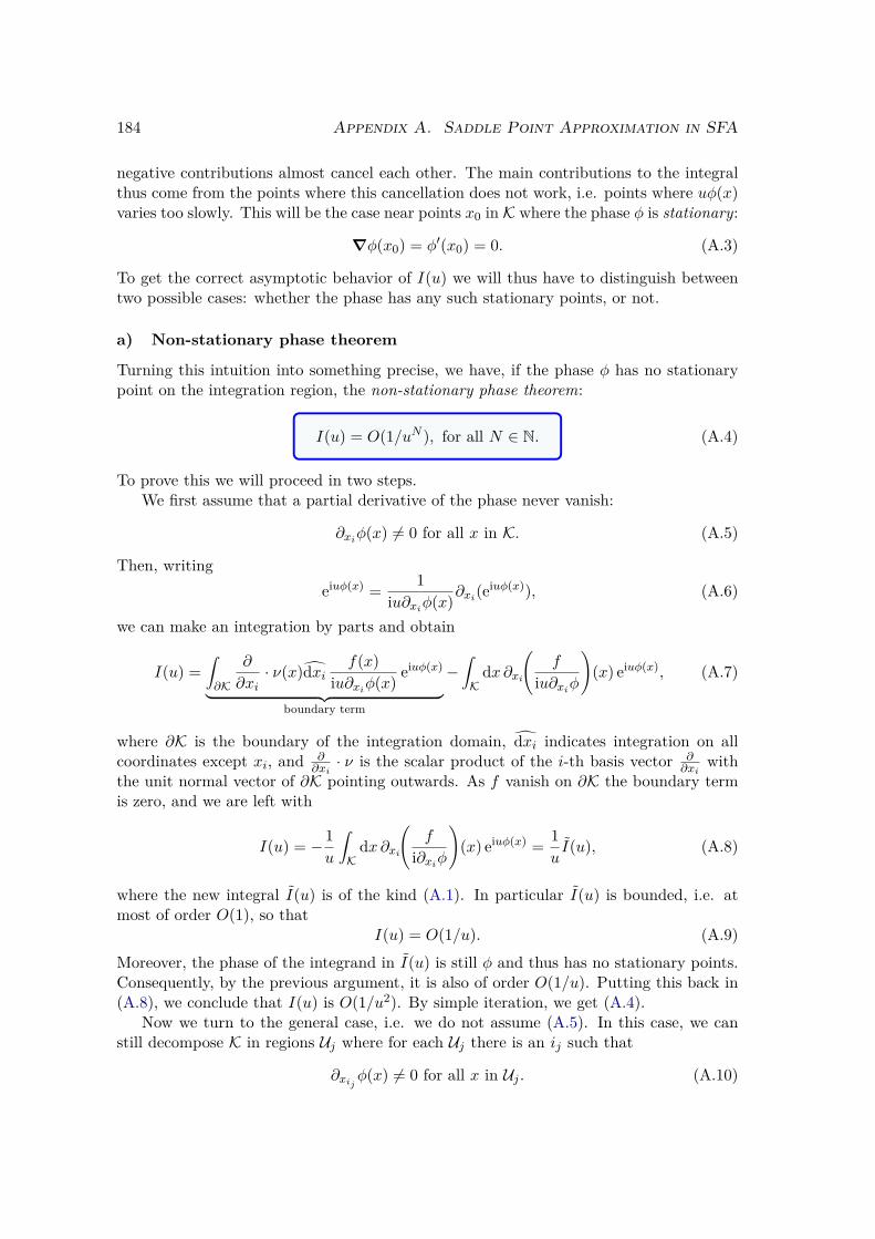
184 Appendix A. Saddle Point Approximation in SFA
negative contributions almost cancel each other. The main contributions to the integralthus come from the points where this cancellation does not work, i.e. points where uφ(x)varies too slowly. This will be the case near points x0 in K where the phase φ is stationary:
∇φ(x0) = φ′(x0) = 0. (A.3)
To get the correct asymptotic behavior of I(u) we will thus have to distinguish betweentwo possible cases: whether the phase has any such stationary points, or not.
a) Non-stationary phase theorem
Turning this intuition into something precise, we have, if the phase φ has no stationarypoint on the integration region, the non-stationary phase theorem:
I(u) = O(1/uN ), for all N ∈ N. (A.4)
To prove this we will proceed in two steps.We first assume that a partial derivative of the phase never vanish:
∂xiφ(x) 6= 0 for all x in K. (A.5)
Then, writingeiuφ(x) = 1
iu∂xiφ(x)∂xi(eiuφ(x)), (A.6)
we can make an integration by parts and obtain
I(u) =∫∂K
∂
∂xi· ν(x)dxi
f(x)iu∂xiφ(x) eiuφ(x)
︸ ︷︷ ︸boundary term
−∫K
dx ∂xi
(f
iu∂xiφ
)(x) eiuφ(x), (A.7)
where ∂K is the boundary of the integration domain, dxi indicates integration on allcoordinates except xi, and ∂
∂xi· ν is the scalar product of the i-th basis vector ∂
∂xiwith
the unit normal vector of ∂K pointing outwards. As f vanish on ∂K the boundary termis zero, and we are left with
I(u) = −1u
∫K
dx ∂xi
(f
i∂xiφ
)(x) eiuφ(x) = 1
uI(u), (A.8)
where the new integral I(u) is of the kind (A.1). In particular I(u) is bounded, i.e. atmost of order O(1), so that
I(u) = O(1/u). (A.9)Moreover, the phase of the integrand in I(u) is still φ and thus has no stationary points.Consequently, by the previous argument, it is also of order O(1/u). Putting this back in(A.8), we conclude that I(u) is O(1/u2). By simple iteration, we get (A.4).
Now we turn to the general case, i.e. we do not assume (A.5). In this case, we canstill decompose K in regions Uj where for each Uj there is an ij such that
∂xijφ(x) 6= 0 for all x in Uj . (A.10)
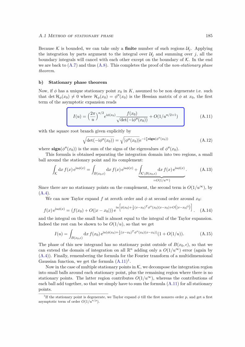
A.1 Method of stationary phase 185
Because K is bounded, we can take only a finite number of such regions Uj . Applyingthe integration by parts argument to the integral over Uj and summing over j, all theboundary integrals will cancel with each other except on the boundary of K. In the endwe are back to (A.7) and thus (A.8). This completes the proof of the non-stationary phasetheorem.
b) Stationary phase theorem
Now, if φ has a unique stationary point x0 in K, assumed to be non degenerate i.e. suchthat detHφ(x0) 6= 0 where Hφ(x0) = φ′′(x0) is the Hessian matrix of φ at x0, the firstterm of the asymptotic expansion reads
I(u) =(2πu
)n/2eiφ(x0) f(x0)√
det(−iφ′′(x0))+O(1/un/2+1) (A.11)
with the square root branch given explicitly by√det(−iφ′′(x0)) =
√|φ′′(x0)|e−iπ4 sign(φ′′(x0)) (A.12)
where sign(φ′′(x0)) is the sum of the signs of the eigenvalues of φ′′(x0).This formula is obtained separating the integration domain into two regions, a small
ball around the stationary point and its complement:∫K
dx f(x) eiuφ(x) =∫B(x0,ε)
dx f(x) eiuφ(x) +∫K\B(x0,ε)
dx f(x) eiuφ(x)
︸ ︷︷ ︸=O(1/u∞)
. (A.13)
Since there are no stationary points on the complement, the second term is O(1/u∞), by(A.4).
We can now Taylor expand f at zeroth order and φ at second order around x0:
f(x) eiuφ(x) =(f(x0) +O(|x− x0|)
)e
iu[φ(x0)+ 1
2 (x−x0)Tφ′′(x0)(x−x0)+O(|x−x0|3
)]. (A.14)
and the integral on the small ball is almost equal to the integral of the Taylor expansion.Indeed the rest can be shown to be O(1/u), so that we get
I(u) =∫B(x0,ε)
dx f(x0) eiu(φ(x0)+ 12 (x−x0)Tφ′′(x0)(x−x0))(1 +O(1/u)). (A.15)
The phase of this new integrand has no stationary point outside of B(x0, ε), so that wecan extend the domain of integration on all Rn adding only a O(1/u∞) error (again by(A.4)). Finally, remembering the formula for the Fourier transform of a multidimensionalGaussian function, we get the formula (A.11)1.
Now in the case of multiple stationary points inK, we decompose the integration regioninto small balls around each stationary point, plus the remaining region where there is nostationary points. The latter region contributes O(1/u∞), whereas the contributions ofeach ball add together, so that we simply have to sum the formula (A.11) for all stationarypoints.
1If the stationary point is degenerate, we Taylor expand φ till the first nonzero order p, and get a firstasymptotic term of order O(1/un/p).
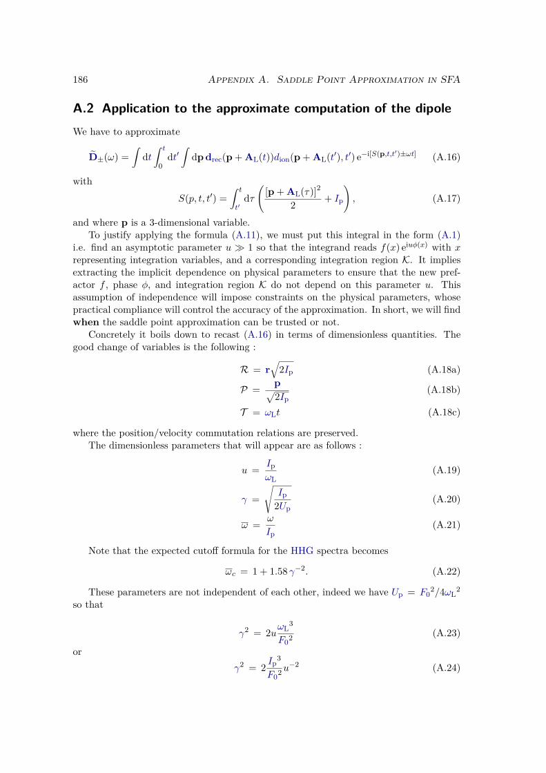
186 Appendix A. Saddle Point Approximation in SFA
A.2 Application to the approximate computation of the dipoleWe have to approximate
D±(ω) =∫
dt∫ t
0dt′∫
dp drec(p + AL(t))dion(p + AL(t′), t′) e−i[S(p,t,t′)±ωt] (A.16)
withS(p, t, t′) =
∫ t
t′dτ(
[p + AL(τ)]2
2 + Ip
), (A.17)
and where p is a 3-dimensional variable.To justify applying the formula (A.11), we must put this integral in the form (A.1)
i.e. find an asymptotic parameter u 1 so that the integrand reads f(x) eiuφ(x) with xrepresenting integration variables, and a corresponding integration region K. It impliesextracting the implicit dependence on physical parameters to ensure that the new pref-actor f , phase φ, and integration region K do not depend on this parameter u. Thisassumption of independence will impose constraints on the physical parameters, whosepractical compliance will control the accuracy of the approximation. In short, we will findwhen the saddle point approximation can be trusted or not.
Concretely it boils down to recast (A.16) in terms of dimensionless quantities. Thegood change of variables is the following :
R = r√
2Ip (A.18a)
P = p√2Ip
(A.18b)
T = ωLt (A.18c)
where the position/velocity commutation relations are preserved.The dimensionless parameters that will appear are as follows :
u = IpωL
(A.19)
γ =√
Ip2Up
(A.20)
ω = ω
Ip(A.21)
Note that the expected cutoff formula for the HHG spectra becomes
ωc = 1 + 1.58 γ−2. (A.22)
These parameters are not independent of each other, indeed we have Up = F02/4ωL
2
so that
γ2 = 2uωL3
F02 (A.23)
orγ2 = 2 Ip
3
F02u−2 (A.24)
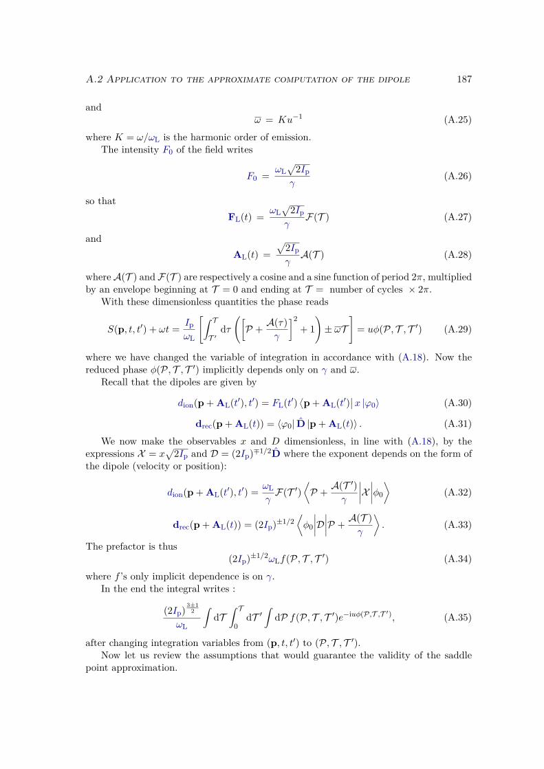
A.2 Application to the approximate computation of the dipole 187
andω = Ku−1 (A.25)
where K = ω/ωL is the harmonic order of emission.The intensity F0 of the field writes
F0 = ωL√
2Ipγ
(A.26)
so thatFL(t) = ωL
√2Ipγ
F(T ) (A.27)
andAL(t) =
√2IpγA(T ) (A.28)
whereA(T ) and F(T ) are respectively a cosine and a sine function of period 2π, multipliedby an envelope beginning at T = 0 and ending at T = number of cycles × 2π.
With these dimensionless quantities the phase reads
S(p, t, t′) + ωt = IpωL
[∫ TT ′
dτ([P + A(τ)
γ
]2+ 1
)± ωT
]= uφ(P, T , T ′) (A.29)
where we have changed the variable of integration in accordance with (A.18). Now thereduced phase φ(P, T , T ′) implicitly depends only on γ and ω.
Recall that the dipoles are given by
dion(p + AL(t′), t′) = FL(t′)⟨p + AL(t′)
∣∣x |ϕ0〉 (A.30)
drec(p + AL(t)) = 〈ϕ0| D |p + AL(t)〉 . (A.31)We now make the observables x and D dimensionless, in line with (A.18), by the
expressions X = x√
2Ip and D = (2Ip)∓1/2D where the exponent depends on the form ofthe dipole (velocity or position):
dion(p + AL(t′), t′) = ωLγF(T ′)
⟨P + A(T ′)
γ
∣∣∣∣X ∣∣∣∣φ0
⟩(A.32)
drec(p + AL(t)) = (2Ip)±1/2⟨φ0
∣∣∣∣D∣∣∣∣P + A(T )γ
⟩. (A.33)
The prefactor is thus(2Ip)±1/2ωLf(P, T , T ′) (A.34)
where f ’s only implicit dependence is on γ.In the end the integral writes :
(2Ip) 3±12
ωL
∫dT
∫ T0
dT ′∫
dP f(P, T , T ′)e−iuφ(P,T ,T ′), (A.35)
after changing integration variables from (p, t, t′) to (P, T , T ′).Now let us review the assumptions that would guarantee the validity of the saddle
point approximation.
188 Appendix A. Saddle Point Approximation in SFA
• u 1 i.e. the ionization potential must be large compared to the frequency of theelectric field.
• γ ∼ 1 ⇐⇒ F02/(2Ip
3) ∼ u2 i.e. the intensity of the electric field must be largecompared to the cube of the ionization potential (but recall that we need γ ≤ 1 fortunnelling to dominate).
• ω ∼ 1 ⇐⇒ K ∼ u i.e. the formula will only be valid for high harmonic orders ofthe emitted spectrum.
So we are looking at the limit of low frequency ωL << Ip, for a strong field γ ≤ 1,and only at the high frequency part of the emitted spectra, where K scales as u−1.
The dimensionless saddle point equation ∇φ(P, T , T ′) = 0 reads
∇Pφ =∫ TT ′
dτ(P + A(τ)
γ
)= 0 (A.36)
∂φ
∂T ′= −(P + A(T ′)
γ)2 − 1 = 0 (A.37)
∂φ
∂T= (P + A(T )
γ)2 + 1± ω = 0. (A.38)
This is simply the dimensionless counterpart of the atomic saddle equations (I.104).We can easily solve the first equation and plug it in the other two:
P(T , T ′) = −γ−1 1(T − T ′)
∫ TT ′
dτ A(τ) (A.39)
[A(T ′)− 1
(T − T ′)
∫ TT ′
dτ A(τ)]2 = −γ2 (A.40)
[A(T )− 1
(T − T ′)
∫ TT ′
dτ A(τ)]2 = −γ2(1± ω). (A.41)
It is clear that equation (A.40) has no real solution T ′. Given that the region ofintegration K is real, we conclude from (A.4) that the integral is O(1/u∞). This iscoherent with the fact that this phenomena relies on tunnelling, which is an exponentiallysmall effect (see chapter III).
Nevertheless we can still compute the first non zero order of the prefactor of this ex-ponential. The general way is to deform the domain of integration in complex coordinates(P, T , T ′), while keeping the integral convergent, so that it passes through a complexsaddle point z0. As the value of a complex analytic integral does not vary when thecontour is deformed, as long as it does not cross singular points of the integrand, thisdeformation process preserves the value of the integral. If the new domain of integrationis chosen carefully, in practice it has to cross the saddle points in directions where thephase has a constant imaginary part, then the integral can be handled by the method ofstationary phase. Indeed close to the saddle points, this constant imaginary part in thephase will result in a real attenuated exponential term (as expected from the previousconsideration) that we can factor out of the integral, and thus be left with an integral ofthe form (A.1).
A.2 Application to the approximate computation of the dipole 189
Note that the saddle point z0 will correspond to a stationary point of the real part ofthe phase Re(φ). Indeed, as hinted by the change of terminology, a stationary point of areal function corresponds to a saddle point of its complex analytic extension.
So the question becomes : find the complex solutions of (A.36), find the appropriatedirections, then try deforming the contour to make it pass through one or several of thesesolutions. Note that the integration domain cannot be deformed at its boundaries sofinding a deformation is not trivial.
Remark that we need to find, among all the saddle points, the ones through which thedeformed integration domain has to pass, i.e. we need to determine which of the saddlepoints contribute to the integral. In general this turns out to be very difficult, especiallyfor multidimensional integrals. More explicitly we need to compute the curves comingfrom a saddle point z0 on which the phase stays real. These curves (the so-called curvesof steepest descents) are of two kinds. The first kind over which the phase has a maximumat z0, and the second kind over which the phase has a minimum at z0. The union of theminimum curves is called a ascending disk (or Lefschetz thimble as in the introduction of[280]), while the union of the maximum curves is an descending disk. Indeed both aredeformed copies of a disk Rn in Cn. Then, the rule reads : a saddle point contributes ifand only if its descending disk intersects the original integration region K.
Here we are in the case K ⊂ Rn+2 ⊂ Cn+2 i.e. in real dimension 2(n + 2), so it isnot generally easy to compute these ascending disks - even with computers. We were notable to do it here.
A more empirical approach is to apply the method of stationary phase first to theP-integral, considering it as an integral with fixed parameters (T , T ′). Since we find onlyone saddle point P(T , T ′) (A.39), we know that is has to contribute to the P-integral.Then we plug the result in the (T , T ′)-integral and apply again the method of stationaryphase.
We compute numerically the complex saddle points (T , T ′) solutions of (A.41),(A.40).They are two of them (TS , T ′S) and (TL, T ′L), corresponding respectively to the small andlong trajectories. Assuming both these saddle points contribute, we apply twice theformula (A.11) and sum the two terms. Eventually - changing back variables - we get theformula (I.107) with the prefactor (I.109).

190 Appendix A. Saddle Point Approximation in SFA
Appendix BFree particle in a grid
We want to find the expression of the energies of a free particle in a grid. The grid isdefined as in section II.1.1: it is composed of Nx points (xj)j=1,Nx ranging from −L to+L and separated by a constant step ∆x. The eigenstates Ψ are solution of
− 12∆x2 Ψ(xj−1) + 1
∆x2 Ψ(xj)−1
2∆x2 Ψ(xj+1) = EΨ(xj). (B.1)
As in the case of a free particle in a box [135], the solutions takes the form of planewaves:
Ψ(xj) = A eikxj +B e−ikxj . (B.2)
This function has to satisfy continuity conditions at borders of the box. The conditionΨ(−L) = 0 forces
A e−ikL +B eikL = 0, (B.3)
which givesΨ(xj) = 2iA e−ikL sin(kxj + kL). (B.4)
The condition Ψ(L) = 0 imposes
k = nπ
2L, n ∈ 0, .., Nx. (B.5)
Inserting (B.4) into (B.1) gives:
E∆x2 sin(kx+ kL) =− 12 sin(kx+ kL− k∆x) + sin(kx+ kL)− 1
2 sin(kx+ kL+ k∆x)
(B.6)
=− 12 sin(kx+ kL) cos(k∆x) +
(((((((
(((((1
2 cos(kx+ kL) sin(k∆x)
+ sin(kx+ kL)
− 12 sin(kx+ kL) cos(k∆x)−
(((((((
(((((1
2 cos(kx+ kL) sin(k∆x) (B.7)
= sin(kx+ kL) [1− cos(k∆x)] (B.8)
=2 sin(kx+ kL) sin2(k∆x
2
). (B.9)
191
192 Appendix B. Free particle in a grid
Using (B.5), we get the final expression for energies:
En = 2∆x2 sin2
(nπ∆x
4L
). (B.10)
We immediately see that the energies do not span all values between 0 and +∞, butreach a maximum at Emax = 2/∆x2. We also see that, when ∆x→ 0 we recover the freeparticle in a box formula:
En −→∆x→0
n2π2
2(2L)2 = k2
2 , (B.11)
from which we can compute the density of states:
ρ(E) = dndE = 2L
π√
2E, (B.12)
where the 2 comes from the degeneracy of the ±n states.
Appendix CStrömgren normalization method
In this appendix we explain, following [271, 281], the Strömgren procedure to normalizeon the energy scale the one dimensional continuum states of an arbitrary even potentialV that vanishes at infinity:
V (x) −→x±→∞
0. (C.1)
These continuum states ϕE are solution of the linear differential equation:ϕ′′E(x) = −2 (E − V (x))ϕE(x), (C.2)
with positive energy E. Since the potential vanishes at infinity, we can define an "asymp-totic region" beyond some limit xa, where the normalized continuum states χE take thegeneral asymptotic form:
χE(x) = 1√πk(x)
sin(θ(x)), if |x| xa (C.3)
where
k(x) = dθdx (C.4)
k −→x→±∞
√2E. (C.5)
In practice, we will compute a solution ϕE of the TISE (C.2) with the RK4 algorithmusing the arbitrary initial conditions given in section II.1.3 c). We then want to determinethe normalization constant C that relates this solution ϕE to the normalized solution χE :
ϕE(x) = 1CχE(x). (C.6)
For this we fit the numeric solution to the asymptotic form (C.3), via the determinationof the function k(x) and θ(x).
We choose in the asymptotic region an interval [x0, x1] on which we know the wavefunction ϕE and define:
a0 =√πk(x0)ϕE(x0) = 1
Csin(θ(x0)) (C.7)
a1 =√πk(x1)ϕE(x1) = 1
Csin(θ(x1)) (C.8)
α =∫ x1
x0k(x) dx = θ(x1)− θ(x0). (C.9)
193
194 Appendix C. Strömgren normalization method
We can express the normalization constant C with these three quantities:sin(α) = sin(θ(x1)) cos(θ(x0))− sin(θ(x0)) cos(θ(x1))cos(α) = cos(θ(x0)) cos(θ(x1)) + sin(θ(x0)) sin(θ(x1))
(C.10)
⇒
sin(α) = Ca1
√1− C2a2
0 − Ca0
√1− C2a2
1
cos(α) =√
1− C2a20
√1− C2a2
1 + C2a0a1
(C.11)
⇒
sin2(α) = C2
[a2
1
(1− C2a2
0
)+ a2
0
(1− C2a2
1
)− 2a0a2
√1− C2a2
0
√1− C2a2
1
]cos(α) =
√1− C2a2
0
√1− C2a2
1 + C2a0a1
(C.12)
⇒ sin2(α) = C2[a2
0 + a21 − 2a0a1 cos(α)
]. (C.13)
Which finally gives:
C =√
sin2(α)a2
0 + a21 − 2a0a1 cos(α) .
(C.14)
To evaluate C, we thus need to compute a0, a1 and α, i.e. evaluate k(x) in the asymptoticregion.
To determine k(x) in the asymptotic region, we insert the normalized wave functionχE(x) in the TISE (C.2). Let us start by the expression of the second derivative:
χ′E(x) = 1√π
[dk− 1
2
dx sin(θ) + k−12 cos(θ) dθ
dx
](C.15)
= 1√π
[dk− 1
2
dx sin(θ) + k12 cos(θ)
](C.16)
χ′′E(x) = 1√π
d2k−12
dx2 sin(θ) +
dk− 12
dx k cos(θ) +
dk 1
2
dx cos(θ)− k32 sin(θ)
(C.17)
=[
d2k−12
dx2 k12 − k2
]χE(x) (C.18)
= −2 (E − V (x))ϕE(x) (using(C.2)) (C.19)
We thus end up with a new differential equation on k:
d2k−12
dx2 k12 − k2 +A = 0, (C.20)
where A = 2 (E − V (x)). We find an approximate solution of this equation in the asymp-totic region, where k varies slowly, by writing:
k2 = A+ d2k−12
dx2 k12 ' A+ d2κ−
12
dx2 κ12 , (C.21)
195
with
κ = A12 (C.22)
dκ− 12
dx = −14
dAdx A
− 54 (C.23)
d2κ−12
dx2 = −14
d2A
dx2 A− 5
4 + 516
(dAdx
)2A−
94 . (C.24)
With this we can express k only as a function of A and its derivatives, or only as a functionof the potential V and its derivatives:
k '
√A− 1
A
d2V
dx2 + 516
( 1A
dVdx
)2.
(C.25)
This last equation allows us to compute k on the interval [x0;x1]. We will then deducethe quantities a0, a1 and α, and finally the normalization constant C. Moreover we willassess the validity of the different approximations by checking the convergence of C fordifferent intervals [x0;x1] further and further away from the origin.

196 Appendix C. Strömgren normalization method
Appendix D
Split-operator algorithm
In this appendix we establish the expression of the error that is made at each time step bythe split-operator algorithm. This error comes from the approximation of the evolutionoperator:
U = e−iH∆t = e−i(T+V )∆t . (D.1)
First we consider the case of the simple decomposition:
U2nd = e−iT∆t e−iV∆t (D.2)
=(1− iT∆t− T 2 ∆t2
2 +O(∆t3
))(1− iV∆t− V 2 ∆t2
2 +O(∆t3
))(D.3)
= 1− i(T + V
)∆t−
(2T V + T 2 + V 2
) ∆t22 +O
(∆t3
)(D.4)
= 1− iH∆t− H2 ∆t22 +
[V , T
]∆t22 +O
(∆t3
)(D.5)
= e−iH∆t +O(∆t2
). (D.6)
As[V , T
]6= 0 we get an error proportional to ∆t2.
197
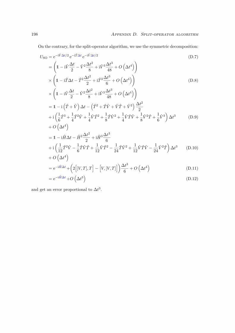
198 Appendix D. Split-operator algorithm
On the contrary, for the split-operator algorithm, we use the symmetric decomposition:
USO = e−iV∆t/2 e−iT∆t e−iV∆t/2 (D.7)
=(1− iV ∆t
2 − V2 ∆t2
8 + iV 3 ∆t348 +O
(∆t4
))
×(1− iT∆t− T 2 ∆t2
2 + iT 3 ∆t36 +O
(∆t4
))(D.8)
×(1− iV ∆t
2 − V2 ∆t2
8 + iV 3 ∆t348 +O
(∆t4
))
= 1− i(T + V
)∆t−
(T 2 + T V + V T + V 2
) ∆t22
+ i(1
6 T3 + 1
4 T2V + 1
4 V T2 + 1
8 T V2 + 1
4 V T V + 18 V
2T + 16 V
3)
∆t3 (D.9)
+O(∆t4
)= 1− iH∆t− H2 ∆t2
2 + iH3 ∆t36
+ i( 1
12 T2V − 1
6 T V T + 112 V T
2 − 124 T V
2 + 112 V T V −
124 V
2T
)∆t3 (D.10)
+O(∆t4
)= e−iH∆t +
(2[[V, T ], T
]−[V, [V, T ]
])∆t36 +O
(∆t4
)(D.11)
= e−iH∆t +O(∆t3
)(D.12)
and get an error proportional to ∆t3.
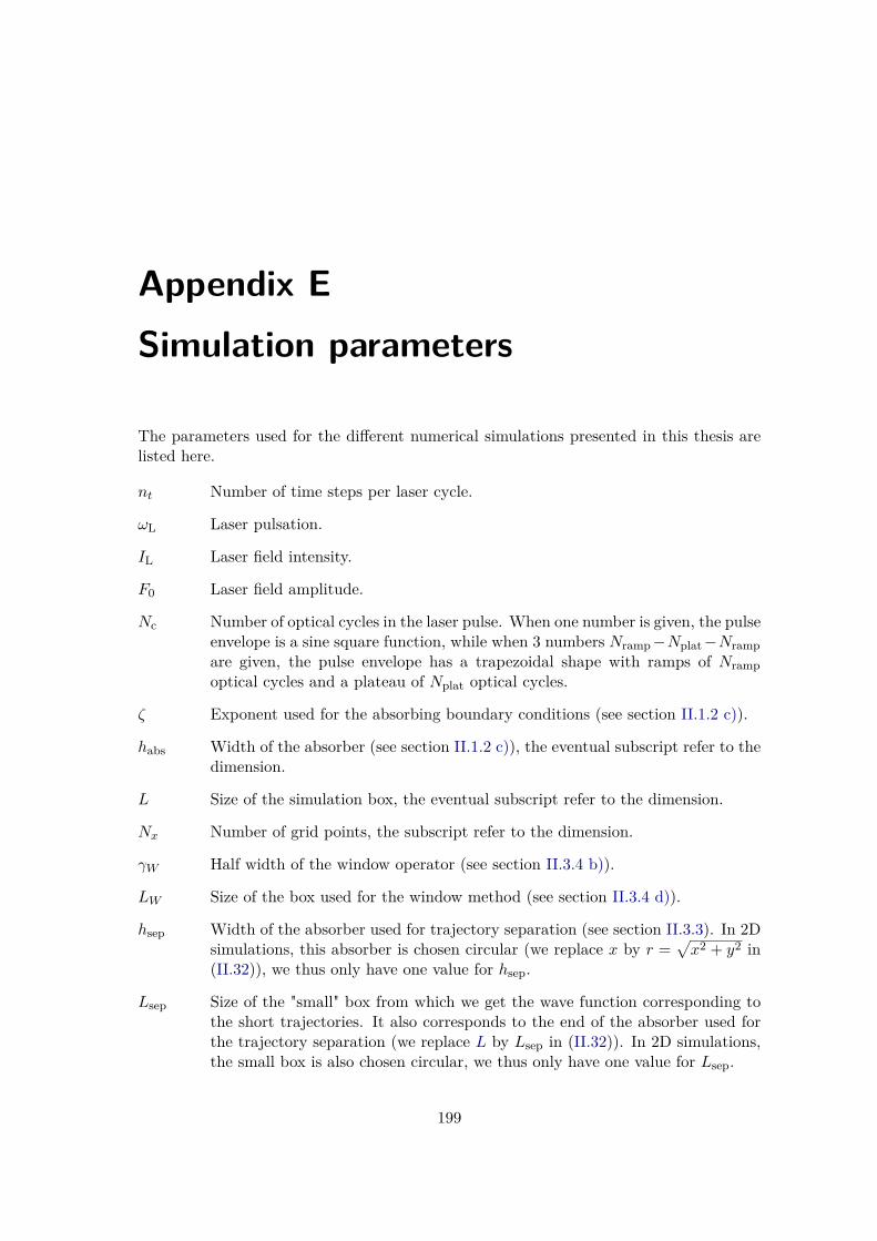
Appendix ESimulation parameters
The parameters used for the different numerical simulations presented in this thesis arelisted here.
nt Number of time steps per laser cycle.
ωL Laser pulsation.
IL Laser field intensity.
F0 Laser field amplitude.
Nc Number of optical cycles in the laser pulse. When one number is given, the pulseenvelope is a sine square function, while when 3 numbers Nramp−Nplat−Nrampare given, the pulse envelope has a trapezoidal shape with ramps of Nrampoptical cycles and a plateau of Nplat optical cycles.
ζ Exponent used for the absorbing boundary conditions (see section II.1.2 c)).
habs Width of the absorber (see section II.1.2 c)), the eventual subscript refer to thedimension.
L Size of the simulation box, the eventual subscript refer to the dimension.
Nx Number of grid points, the subscript refer to the dimension.
γW Half width of the window operator (see section II.3.4 b)).
LW Size of the box used for the window method (see section II.3.4 d)).
hsep Width of the absorber used for trajectory separation (see section II.3.3). In 2Dsimulations, this absorber is chosen circular (we replace x by r =
√x2 + y2 in
(II.32)), we thus only have one value for hsep.
Lsep Size of the "small" box from which we get the wave function corresponding tothe short trajectories. It also corresponds to the end of the absorber used forthe trajectory separation (we replace L by Lsep in (II.32)). In 2D simulations,the small box is also chosen circular, we thus only have one value for Lsep.
199
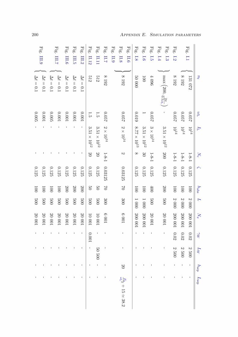
200 Appendix E. Simulation parametersnt
ωL
ILN
cζ
habs
LNx
γW
LW
hsep
Lsep
Fig.I.1
131
0720.057
10 141-8-1
0.125100
2000
200001
0.022500
--
8192
0.05710 14
1-8-10.125
1002000
200001
0.022500
--
Fig.I.2
8192
0.05710 14
1-8-10.125
1002000
200001
0.022500
--
Fig.I.3
m
ax (200,
2π
0.1ω
L )-
3.51×
10 12200
0.125200
50020
001-
--
-Fig.
I.4Fig.
I.54096
0.0573×
10 141-8-1
0.125400
50020
001-
--
-Fig.
I.6100
13.51×
10 1230
0.125100
1000
200001
--
--
Fig.I.8
50000
0.0198.77×
10 138
0.125100
1000
200001
--
--
Fig.II.6
8192
0.0572×
10 142
0.0312570
3006001
--
20F
0ω
L2
+15'
38.2Fig.
II.8Fig.
II.9Fig.
II.78192
0.0572×
10 141-8-1
0.0312570
3006001
--
--
Fig.II.11
5121.5
3.51×
10 1220
0.12550
50010
001-
50500
--
Fig.II.12
5121.5
3.51×
10 1220
0.12550
50010
0010.001
--
-
Fig.III.2
∆t=
0.10.001
--
0.125200
50020
001-
--
-Fig.
III.5∆t=
0.10.001
--
0.125200
50020
001-
--
-Fig.
III.6∆t=
0.10.001
--
0.125200
50020
001-
--
-
Fig.III.7
∆t=
0.10.001
--
0.125100
50020
001-
--
-∆t=
0.10.005
--
0.125100
50020
001-
--
-
Fig.III.9
∆t=
0.10.001
--
0.125100
50020
001-
--
-∆t=
0.10.005
--
0.125100
50020
001-
--
-
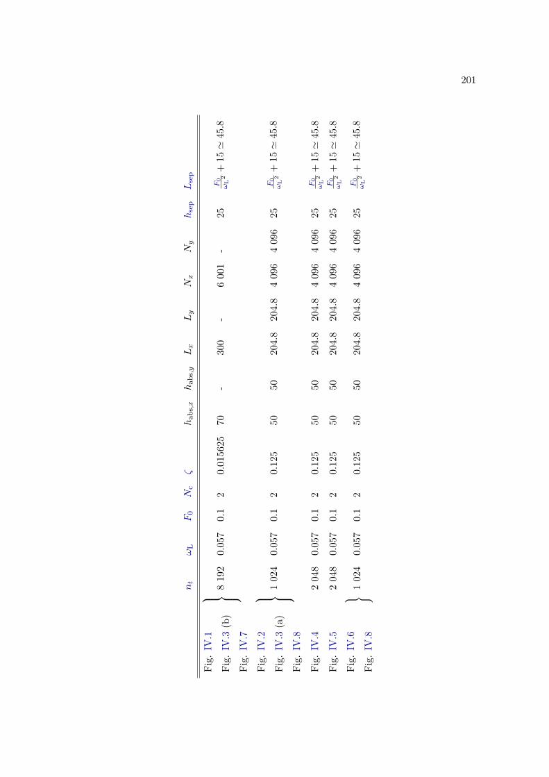
201
nt
ωL
F0
Nc
ζh
abs,x
hab
s,y
Lx
Ly
Nx
Ny
hse
pL
sep
Fig.
IV.1
819
20.05
70.1
20.01
5625
70-
300
-600
1-
25F
0ω
L2
+15'
45.8
Fig.
IV.3
(b)
Fig.
IV.7
Fig.
IV.2
102
40.05
70.1
20.12
550
5020
4.8
204.8
409
6409
625
F0
ωL
2+
15'
45.8
Fig.
IV.3
(a)
Fig.
IV.8
Fig.
IV.4
204
80.05
70.1
20.12
550
5020
4.8
204.8
409
6409
625
F0
ωL
2+
15'
45.8
Fig.
IV.5
204
80.05
70.1
20.12
550
5020
4.8
204.8
409
6409
625
F0
ωL
2+
15'
45.8
Fig.
IV.6
102
40.05
70.1
20.12
550
5020
4.8
204.8
409
6409
625
F0
ωL
2+
15'
45.8
Fig.
IV.8
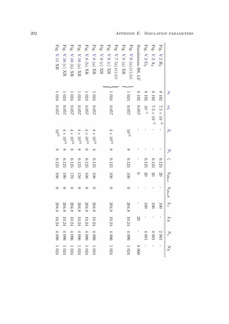
202 Appendix E. Simulation parameters
nt
ωL
ILN
cζ
habs,x
habs,R
Lx
LR
Nx
NR
Fig.V.2
H2
8192
7.5×
10−
2-
-0.125
20-
100-
2001
-Fig.
V.2
A2
8192
7.5×
10−
2-
-0.125
20-
100-
4001
-Fig.
V.2
G2
8192
10−
4-
-0.125
20-
100-
4001
-Sim
ulationsBS,LF
8192
0.057-
--
0-
-20
-8000
Fig.V.6
(a),(c),(e)
1024
0.05710 14
80.125
1000
204.810.24
4096
1024
Fig.V.8
(a)XR
Fig.V.7
(a),(c),(e)
1024
0.0574×
10 148
0.125100
0204.8
10.244096
1024
Fig.V.8
(c)XR
Fig.V.9
(c)XR
Fig.V.8
(a)XR
1024
0.0574×
10 144
0.125100
0204.8
10.244096
1024
Fig.V.8
(b)XR
1024
0.0574×
10 146
0.125100
0204.8
10.244096
1024
Fig.V.10
(a)XR
1024
0.0574×
10 148
0.125150
0204.8
10.244096
1024
Fig.V.10
(b)XR
1024
0.0574×
10 148
0.125170
0204.8
10.244096
1024
Fig.V.10
(c)XR
1024
0.0574×
10 148
0.125190
0204.8
10.244096
1024
Fig.V.11
XR
1024
0.05710 15
80.125
1000
204.810.24
4096
1024
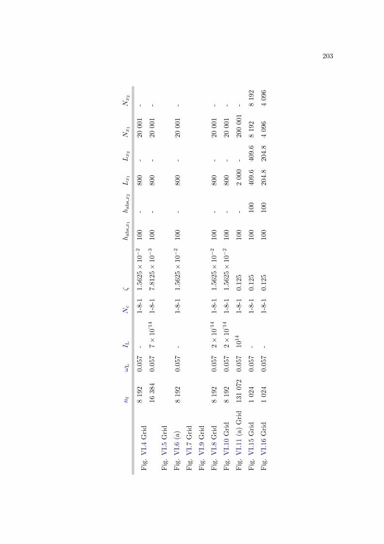
203
nt
ωL
I LN
cζ
hab
s,x
1h
abs,x
2Lx
1Lx
2Nx
1Nx
2
Fig.
VI.4
Grid
819
20.05
7-
1-8-1
1.56
25×
10−
210
0-
800
-20
001
-16
384
0.05
77×
10‘14
1-8-1
7.81
25×
10−
310
0-
800
-20
001
-Fig.
VI.5
Grid
819
20.05
7-
1-8-1
1.56
25×
10−
210
0-
800
-20
001
-Fig.
VI.6
(a)
Fig.
VI.7
Grid
Fig.
VI.9
Grid
Fig.
VI.8
Grid
819
20.05
72×
10‘14
1-8-1
1.56
25×
10−
210
0-
800
-20
001
-Fig.
VI.1
0Grid
819
20.05
72×
10‘14
1-8-1
1.56
25×
10−
210
0-
800
-20
001
-Fig.
VI.1
1(a)Grid
13107
20.05
710
141-8-1
0.12
510
0-
200
0-
20000
1-
Fig.
VI.1
5Grid
102
40.05
7-
1-8-1
0.12
510
010
040
9.6
409.6
819
2819
2Fig.
VI.1
6Grid
102
40.05
7-
1-8-1
0.12
510
010
020
4.8
204.8
409
6409
6

204 Appendix E. Simulation parameters
French Summary
S.1 Introduction
La lumière et la matière sont parmi les objets les plus étudiés par les physiciens. Ilspeuvent interagir de tant de façons différentes qu’ils ouvrent des possibilités pour ainsi direinfinies. Ces interactions sont à l’origine d’un des domaines les plus riches et les plus actifsde la physique, mais présentent également un nombre toujours croissant d’applicationsen permettant de développer des techniques expérimentales toujours plus poussées. Undes exemples les plus marquants est l’utilisation de l’émission stimulée, qui provient del’interaction d’un atome avec un photon, et qui est à la base du laser (Light Amplificationby Stimulated Emission of Radiation, i.e. amplification de lumière par émission stimulée derayonnement) que l’on retrouve désormais dans tous les laboratoires, des tables optiquesjusque dans les salles de conférences.
L’incroyable succès du laser en tant qu’outil universel pour un large éventail d’ap-plications expérimentales provient de ses propriétés fondamentales. C’est une source delumière monochromatique, intense, mais surtout cohérente. Cette dernière particularitéen fait l’outil idéal pour étudier les propriétés quantiques fondamentales de la matière.Depuis l’invention pionnière du maser (Microwave Amplification by Stimulated Emissionof Radiation, i.e. Amplification de micro-ondes par émission stimulée de rayonnement)dans les années 1950, suivie du développement du laser dans les années 1960, d’impor-tants efforts ont permis d’améliorer les différentes caractéristiques de cette célèbre sourcelumineuse. De nouvelles bandes de longueur d’onde peuvent désormais être émises, et cer-tains lasers peuvent même accorder leur longueur d’onde sur certaines plages spectrales.L’intensité émise a été augmentée de plusieurs ordres de grandeur, ce qui a ouvert la voieà la physique des champs forts [1]. En particulier, l’invention de l’amplification par dérivede fréquence (Chirped Pulse Amplification) [2] a été une incroyable percée pour la généra-tion d’impulsion laser de forte intensité. Les impulsions lasers ont également vu leur duréeréduite jusqu’aux limites de la transformée de Fourier. Ces impulsions qui ne dure pas plusd’un cycle laser peuvent atteindre quelques femtosecondes seulement (1 fs = 10−15 s).Cet incroyable réussite est à l’origine de la femtochimie, dont les expériences pionnièresde Zewail [3, 4] ont permis d’étudier à des échelles de temps aussi rapides des dynamiquesmoléculaires, c’est à dire des réactions chimiques.
Ces avancées techniques, et en particulier la possibilité d’atteindre des champs laserstrès intenses (de 1014 W.cm−2 à 1022 W.cm−2) ont conduit à la découverte de processusphysiques fortement non linéaires comme l’ionisation au dessus du seuil (ATI) en 1979 [5],l’ionisation multiple non séquentielle en 1982 [6], ou la génération d’harmoniques d’ordre
205
206 FRENCH SUMMARY
élevé (HHG) par deux groupes différents en 1987 [7] et en 1988 [8]. Ces découvertes ontinduit un fort développement de travaux théoriques pour construire des modèles et mettreau point des mécanismes pour expliquer ces processus [9–11], ce qui reste encore aujour-d’hui un domaine de recherche très actif. Mais au delà de son intérêt physique fondamental,la génération d’harmonique a engendré une véritable révolution. Elle a permis de générerdes impulsions lumineuses cohérentes dans le domaine des extrêmes ultra-violets (XUV),ce qui reste impossible pour les lasers optiques actuels, avec les durées d’impulsion lesplus courtes jamais produites. Ces impulsions peuvent durer seulement quelques dizainesd’attosecondes (1 as = 10−18 s) [12–14], le record mondial actuel étant de 43 as [15],et offrent donc la possibilité d’étudier des dynamiques électroniques à leurs échelles detemps naturelles.
Cette nouvelle source lumineuse est à l’origine d’un tout nouveau domaine de lascience : la physique attoseconde [16–19]. Elle a été utilisée pour mesurer des délaisattosecondes de photoionisation dans des gaz rare comme le Néon [20] et l’argon [21],mais aussi dans des systèmes plus complexes comme des molécules chirales [22] et dessolides [23, 24]. La dynamique de processus fondamentaux comme le déclin Auger [25]ou l’ionisation tunnel [26] a pu être étudiée expérimentalement. Des dynamiques électro-niques ont pu être reconstruite avec une résolution attoseconde dans des atomes [27], desmolécules [28] et des solides [29–31]. Des corrélations électroniques dynamiques ont été ob-servées par la dynamique attoseconde d’une résonance de Fano dans l’hélium [32, 33]. Desdynamiques nucléaire sub-femtosecondes ont pu être mesurées dans des molécules [34].La physique attoseconde s’étend même aujourd’hui aux nano-structures [35–37], pour les-quelles les champs proches, qui proviennent de leur interaction avec le champ incident,ont pu être utilisés pour mesurer et contrôler la dynamique et la diffusion d’électrons àl’échelle attoseconde [38–40].
En plus de ses propriétés remarquables qui en ont fait une source lumineuse incon-tournable, la lumière émise par la génération d’harmoniques contient aussi énormémentd’informations sur le système qui a lui-même émit cette lumière. Cela a contribué audéveloppement d’un nouveau type de spectroscopie qui repose sur la génération d’harmo-niques en tant qu’auto-sonde [41]. Cette technique permet de mesurer des dynamiquesnucléaires attosecondes [42–44], d’imager des paquets d’onde électroniques dépendants dutemps [45], de reconstruire les orbitales du système par tomographie [46–48], de suivre desdynamiques poly-électroniques dans des atomes [49], des molécules [50] et des solides [51],de distinguer les énantiomères d’une molécule chirale [55], ou de révéler des symétriesdynamiques dans des atomes et des molécules [56].
Ces avancées passionnantes poussent au développement de méthodes théoriques etnumériques poussées pour analyser, interpréter, et préparer toutes ces expériences. Eneffet l’interaction entre atomes et photons est souvent comprise par l’intermédiaire de latrès puissante théorie des perturbations dépendante du temps. Cependant cette méthodene permet de modéliser que les processus linéaires, ou modérément non linéaire, que l’onobserve en présence de champs relativement peu intenses. Dans le cas de la générationd’harmoniques, ou d’autre processus fortement non linéaires, l’intensité du laser incidentest comparable au potentiel d’interaction entre les électrons et les noyaux. Celui-ci nepeux donc pas être considéré comme une perturbation. La description théorique de ladynamiques électroniques en présence de tels champs lasers nécessite donc de résoudre
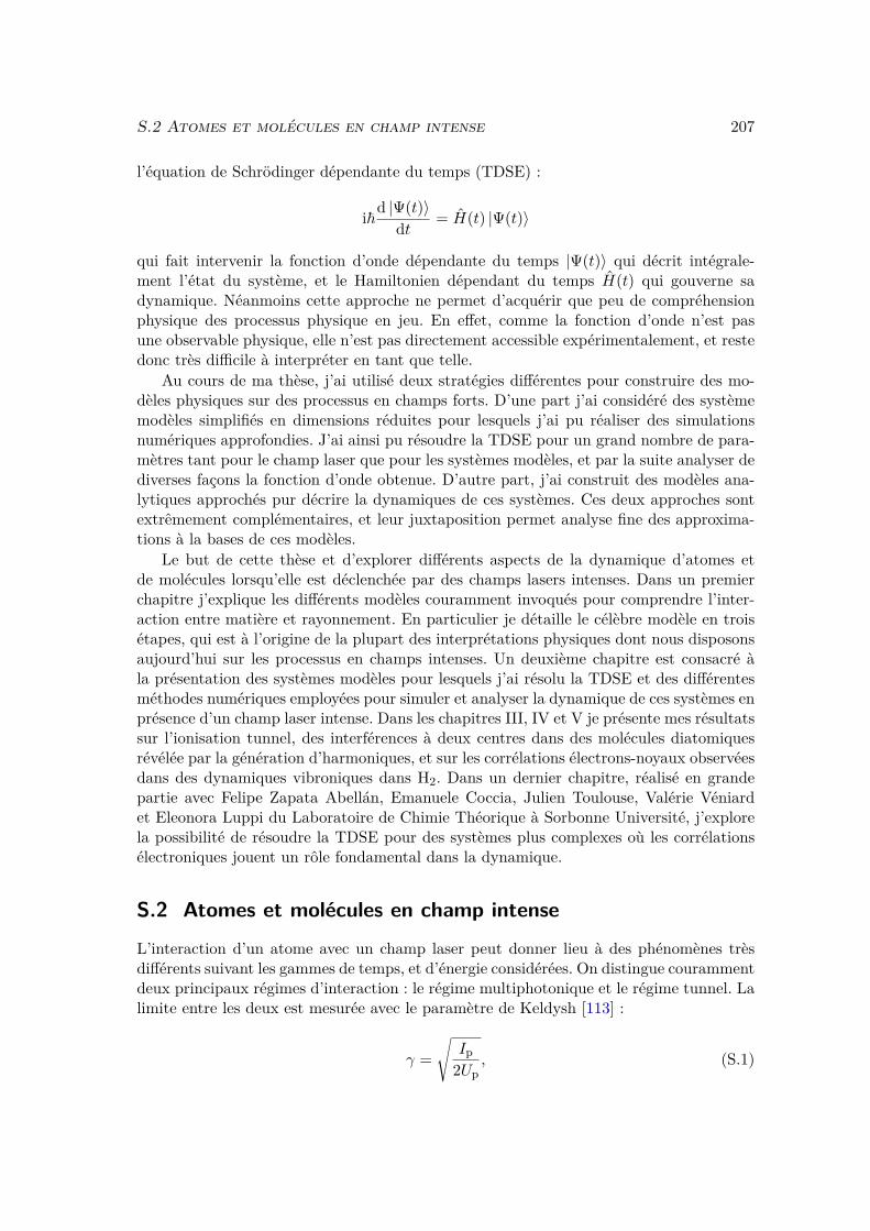
S.2 Atomes et molécules en champ intense 207
l’équation de Schrödinger dépendante du temps (TDSE) :
i~d |Ψ(t)〉dt = H(t) |Ψ(t)〉
qui fait intervenir la fonction d’onde dépendante du temps |Ψ(t)〉 qui décrit intégrale-ment l’état du système, et le Hamiltonien dépendant du temps H(t) qui gouverne sadynamique. Néanmoins cette approche ne permet d’acquérir que peu de compréhensionphysique des processus physique en jeu. En effet, comme la fonction d’onde n’est pasune observable physique, elle n’est pas directement accessible expérimentalement, et restedonc très difficile à interpréter en tant que telle.
Au cours de ma thèse, j’ai utilisé deux stratégies différentes pour construire des mo-dèles physiques sur des processus en champs forts. D’une part j’ai considéré des systèmemodèles simplifiés en dimensions réduites pour lesquels j’ai pu réaliser des simulationsnumériques approfondies. J’ai ainsi pu résoudre la TDSE pour un grand nombre de para-mètres tant pour le champ laser que pour les systèmes modèles, et par la suite analyser dediverses façons la fonction d’onde obtenue. D’autre part, j’ai construit des modèles ana-lytiques approchés pur décrire la dynamiques de ces systèmes. Ces deux approches sontextrêmement complémentaires, et leur juxtaposition permet analyse fine des approxima-tions à la bases de ces modèles.
Le but de cette thèse et d’explorer différents aspects de la dynamique d’atomes etde molécules lorsqu’elle est déclenchée par des champs lasers intenses. Dans un premierchapitre j’explique les différents modèles couramment invoqués pour comprendre l’inter-action entre matière et rayonnement. En particulier je détaille le célèbre modèle en troisétapes, qui est à l’origine de la plupart des interprétations physiques dont nous disposonsaujourd’hui sur les processus en champs intenses. Un deuxième chapitre est consacré àla présentation des systèmes modèles pour lesquels j’ai résolu la TDSE et des différentesméthodes numériques employées pour simuler et analyser la dynamique de ces systèmes enprésence d’un champ laser intense. Dans les chapitres III, IV et V je présente mes résultatssur l’ionisation tunnel, des interférences à deux centres dans des molécules diatomiquesrévélée par la génération d’harmoniques, et sur les corrélations électrons-noyaux observéesdans des dynamiques vibroniques dans H2. Dans un dernier chapitre, réalisé en grandepartie avec Felipe Zapata Abellán, Emanuele Coccia, Julien Toulouse, Valérie Véniardet Eleonora Luppi du Laboratoire de Chimie Théorique à Sorbonne Université, j’explorela possibilité de résoudre la TDSE pour des systèmes plus complexes où les corrélationsélectroniques jouent un rôle fondamental dans la dynamique.
S.2 Atomes et molécules en champ intense
L’interaction d’un atome avec un champ laser peut donner lieu à des phénomènes trèsdifférents suivant les gammes de temps, et d’énergie considérées. On distingue courammentdeux principaux régimes d’interaction : le régime multiphotonique et le régime tunnel. Lalimite entre les deux est mesurée avec le paramètre de Keldysh [113] :
γ =√
Ip2Up
, (S.1)
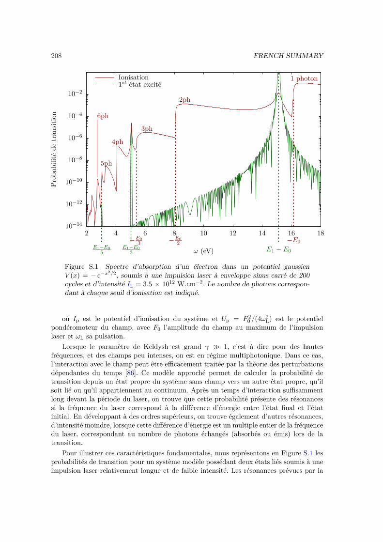
208 FRENCH SUMMARY
10−14
10−12
10−10
10−8
10−6
10−4
10−2
2 4 6 8 10 12 14 16 18
3ph
2ph
1 photon
4ph
5ph
6ph
−E03 −E0
2 −E0E1 − E0
E1−E03
E1−E05
Prob
abilité
detran
sition
ω (eV)
Ionisation1st état excité
Figure S.1 Spectre d’absorption d’un électron dans un potentiel gaussienV (x) = − e−x2/2, soumis à une impulsion laser à enveloppe sinus carré de 200cycles et d’intensité IL = 3.5 × 10¹² W.cm−2. Le nombre de photons correspon-dant à chaque seuil d’ionisation est indiqué.
où Ip est le potentiel d’ionisation du système et Up = F 20 /(4ω2
L) est le potentielpondéromoteur du champ, avec F0 l’amplitude du champ au maximum de l’impulsionlaser et ωL sa pulsation.
Lorsque le paramètre de Keldysh est grand γ 1, c’est à dire pour des hautesfréquences, et des champs peu intenses, on est en régime multiphotonique. Dans ce cas,l’interaction avec le champ peut être efficacement traitée par la théorie des perturbationsdépendantes du temps [86]. Ce modèle approché permet de calculer la probabilité detransition depuis un état propre du système sans champ vers un autre état propre, qu’ilsoit lié ou qu’il appartiennent au continuum. Après un temps d’interaction suffisammentlong devant la période du laser, on trouve que cette probabilité présente des résonancessi la fréquence du laser correspond à la différence d’énergie entre l’état final et l’étatinitial. En développant à des ordres supérieurs, on trouve également d’autres résonances,d’intensité moindre, lorsque cette différence d’énergie est un multiple entier de la fréquencedu laser, correspondant au nombre de photons échangés (absorbés ou émis) lors de latransition.
Pour illustrer ces caractéristiques fondamentales, nous représentons en Figure S.1 lesprobabilités de transition pour un système modèle possédant deux états liés soumis à uneimpulsion laser relativement longue et de faible intensité. Les résonances prévues par la
S.2 Atomes et molécules en champ intense 209
(a)
|ϕ0〉
V0 + xFL(t)
(b)(b) (c)
ωe
Figure S.2 Représentation schématique du modèle en trois étapes : (a) ionisa-tion tunnel, (b) accélération par le champ et retour à proximité des noyaux, (c)recombinaison et émission d’un photon XUV.
théorie des perturbations dépendante du temps sont indiquées sur la figure. Certainestransitions sont cependant absentes : par exemple on n’observe aucune résonance pourun photon d’énergie ωL = (E1 − E0)/2. Ceci est du à des règles de sélections imposéespar la symétrie des états initiaux et finaux et par le nombre de photons mis en jeu dansla transition.
Au contraire dans le cas où le paramètre de Keldysh est petit γ 1, c’est à dire pourdes faibles fréquences, et en champ intense, on est en régime tunnel. Dans ce cas le champlaser intense ne peut pas être considéré comme une perturbation. Néanmoins commela fréquence du laser est faible comparée aux échelles de temps caractéristiques de ladynamique électronique, on peut considérer que l’électron suit adiabatiquement le champélectrique. C’est à dire qu’on suppose que l’électron réagit instantanément à la valeur queprend le champ à chaque instant. On peut donc regarder le potentiel effectif, constituédu potentiel d’interaction avec les noyaux et de l’interaction avec le champ, que ressentl’électron à un temps t. Ceci est représenté schématiquement en Figure S.2 (a) : on voitapparaître une barrière de potentiel au travers de laquelle l’électron va pouvoir s’échapperpar effet tunnel, créant un paquet d’onde électronique dans le continuum. À un instantultérieur, lorsque la valeur instantanée du champ a changé de signe, ce paquet d’onde estramené proche du cœur ionique dont il est parti, comme illustré en Figure S.2 (b). Lorsquece paquet d’onde se retrouve à proximité des noyaux, il y a une probabilité non nulle pourqu’il se recombine avec l’état fondamental, comme schématisé en Figure S.2 (c), et qu’illibère ainsi toute l’énergie cinétique accumulée lors de son trajet dans le continuum enémettant un photon. Ces trois processus (a) ionisation tunnel, (b) propagation dans lecontinuum et accélération par le champ et (c) recombinaison constituent le fameux modèleen trois étapes [9, 10, 91, 11]. Le processus dans son ensemble est appelé la générationd’harmoniques d’ordre élevé (HHG). Il se répète à chaque demi cycle laser de part etd’autres des noyaux. Le rayonnement émis présente des caractéristiques très spécifiques.Il présent un spectre très large constitué des harmoniques du rayonnement laser incident,
210 FRENCH SUMMARY
et, dans le cas où le système présente un centre d’inversion, uniquement des harmoniquesimpaires. Dans le domaine temporel, il prend la forme d’un train d’impulsions laserspouvant durer chacune quelques dizaines d’attosecondes seulement. De plus, comme lesélectrons ayant suivis différentes trajectoires lors de la seconde étape (b) ont tous le mêmeétat final et initial, il peuvent interférer entre eux. Ces interférences encodent beaucoupd’informations sur le système et apparaissent également dans le spectre de la lumièreémise.
S.3 Ionisation tunnel
L’ionisation tunnel fut en premier lieu modélisée par Keldysh [113], et a depuis fait l’at-tention d’un grand nombre de travaux théoriques. Comme pour beaucoup de processusfortement non linéaire, la seule manière de décrire précisément l’ionisation tunnel est derésoudre la TDSE. Comme cela nécessite d’importantes ressources numériques, les théori-ciens ont souvent recours à différentes approximations pour simplifier les systèmes traités,ou à des méthodes analytiques approchées. Parmi ces méthodes analytiques, les plus cou-ramment utilisées sont les formules obtenues par Ammosov, Delone et Krainov [177] et parPerelomov, Popov et Terent’ev [174] pour les atomes, et étendues aux molécules par Tonget al. [178, 179] et Kjeldsen et Madsen [180]. Ces formules reposent toutes sur l’approxi-mation adiabatique et sont donc déduites de la formule en champ statique obtenue parLandau et Lifshitz pour l’atome d’hydrogène [132] et généralisée par Smirnov et Chibisov(SC) [184].
Cependant ces formules sont uniquement valides pour un champ asymptotiquementfaible F → 0 et ont donc une précision limitée pour des champs non nuls. En comparantles résultats données par la formule de Smirnov et Chibisov et des résultats "exacts",à la précision numérique près, j’ai montré dans ma thèse que la compensation d’erreurjouait un rôle fondamental dans l’accord résultats analytiques et numériques. J’ai éga-lement établi une formule corrigée qui tient compte de l’effet du champ laser sur lesniveaux d’énergies dy système, ce qui est couramment appelé l’effet Stark. Correctionpermet d’améliorer considérablement la précision de la formule SC. La contribution del’effet Stark est même indispensable pour reproduire le comportement qualitatif de l’io-nisation de molécules polaires. Pour les atomes et pour certaines molécules peu polairesl’effet Stark peut être calculé par la théorie des perturbations indépendantes du temps audeuxième ordre (2PT). Ceci est illustré en Figure S.3 (a) : l’accord entre la formule SC etles calculs numérique "TDSE" se détériore quand le champ s’intensifie. Pour cette petitemolécule, la théorie des perturbations au second ordre (2PT) permet de corriger la for-mule et d’améliorer l’accord. Néanmoins dans le cas de molécules très polarisable, commecelle présentée en Figure S.3 (b) il est nécessaire d’utiliser la théorie des perturbationsindépendante du temps dégénérée pour obtenir un accord acceptable.
S.4 Interférences à deux centres observées par la générationd’harmoniques d’ordres élevés
La génération d’harmoniques n’est pas qu’une source lumineuse. Elle permet égalementd’avoir accès à nombre d’informations tant structurelles que dynamiques sur le système
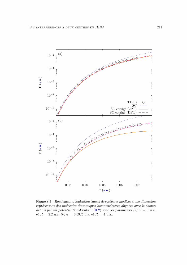
S.4 Interférences à deux centres en HHG 211
10−10
10−8
10−6
10−4
10−2 (a)
10−10
10−8
10−6
10−4
10−2
0.03 0.04 0.05 0.06 0.07
(b)
Γ(a.u.)
TDSESC
SC corrigé (2PT)SC corrigé (DPT)
Γ(a.u.)
F (a.u.)
Figure S.3 Rendement d’ionisation tunnel de systèmes modèles à une dimensionreprésentant des molécules diatomiques homonucléaires alignées avec le champdéfinis par un potentiel Soft-Coulomb(II.2) avec les paramètres (a) a = 1 u.a.et R = 2.2 u.a. (b) a = 0.6925 u.a. et R = 4 u.a..
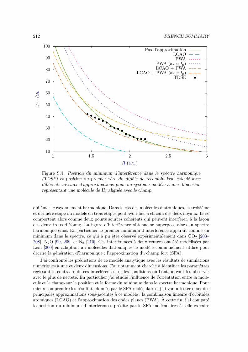
212 FRENCH SUMMARY
10
20
30
40
50
60
70
80
90
100
1 1.5 2 2.5 3
ωm
in/ω
L
R (a.u.)
Pas d’approximationLCAOPWA
PWA (avec Ip)LCAO + PWA
LCAO + PWA (avec Ip)TDSE
Figure S.4 Position du minimum d’interférence dans le spectre harmonique(TDSE) et position du premier zéro du dipôle de recombinaison calculé avecdifférents niveaux d’approximations pour un système modèle à une dimensionreprésentant une molécule de H2 alignée avec le champ.
qui émet le rayonnement harmonique. Dans le cas des molécules diatomiques, la troisièmeet dernière étape du modèle en trois étapes peut avoir lieu à chacun des deux noyaux. Ils secomportent alors comme deux points sources cohérents qui peuvent interférer, à la façondes deux trous d’Young. La figure d’interférence obtenue se superpose alors au spectreharmonique émis. En particulier le premier minimum d’interférence apparait comme unminimum dans le spectre, ce qui a pu être observé expérimentalement dans CO2 [203–208], N2O [99, 209] et N2 [210]. Ces interférences à deux centres ont été modélisées parLein [200] en adaptant au molécules diatomiques le modèle communément utilisé pourdécrire la génération d’harmonique : l’approximation du champ fort (SFA).
J’ai confronté les prédictions de ce modèle analytique avec les résultats de simulationsnumériques à une et deux dimensions. J’ai notamment cherché à identifier les paramètresrégissant le contraste de ces interférences, et les conditions où l’ont pouvait les observeravec le plus de netteté. En particulier j’ai étudié l’influence de l’orientation entre la molé-cule et le champ sur la position et la forme du minimum dans le spectre harmonique. Pourmieux comprendre les résultats donnés par le SFA moléculaires, j’ai voulu tester deux desprincipales approximations sous-jacentes à ce modèle : la combinaison linéaire d’orbitalesatomiques (LCAO) et l’approximation des ondes planes (PWA). À cette fin, j’ai comparéla position du minimum d’interférences prédite par le SFA moléculaires à celle extraite
S.5 Dynamiques vibroniques de molécules en champ intense 213
des simulations numériques. Ces résultats sont montrés en Figure S.4 : les prédictions duSFA moléculaire (en traits brisés jaunes) surestiment de quelques harmoniques la positiondu minimum extraite du spectre des simulations numériques "TDSE" (en points noirs).Une correction empirique impliquant un décalage des énergies du continuum de Ip (entraits brisés oranges) semble améliorer légèrement l’accord entre les deux. Cependant sil’on regarde les prédictions du même modèle, avec la PWA mais sans faire l’approxima-tion LCAO (pointillés roses) on voit que, paradoxalement, les prédictions du modèles sedégradent. De même, si on garde l’approximation LCAO, mais qu’on s’affranchit de laPWA (pointillés bleus), le SFA moléculaire donne de très mauvais résultats. Lorsqu’on nefait aucune des deux approximations, ni la PWA ni la LCAO, (en ligne pleine verte) onretrouve un très bon accord avec les simulations numériques. Cela indique que les erreurscausées par chacune de ces deux approximations se compensent presque parfaitement,donnant l’illusion d’un bon accord entre modèle analytique et simulations numériques.Néanmoins, aucune des deux approximations sous-jacente à ce modèle n’est véritablementjustifiée Cela montre donc que les prédictions du SFA moléculaire, bien qu’apparemmentraisonnables, sont en réalité à prendre avec beaucoup de précautions, surtout à des finquantitatives.
S.5 Dynamiques vibroniques de molécules en champ intense
Lorsque les noyaux de la molécule considérée sont suffisamment légers, alors leur dyna-mique ne peut être négligée même durant les impulsions extrêmement courtes, de quelquesfemtosecondes, que nous avons considérées jusqu’alors. Récemment, ces dynamiques nu-cléaires femtosecondes ont été observées expérimentalement dans D2 [222]. Sous l’effetd’une impulsion laser femtoseconde infrarouge, un paquet d’onde vibrationnel cohérent apu être créé dans l’état électronique fondamental de D2 dont les vibrations ont ensuite puêtre mesurées. Toutefois, cette expérience pose la question du mécanisme physique ayantcréé ce paquet d’onde. En effet, pour une molécule diatomique homonocléaire, le champlaser ne couple pas les différents niveaux vibrationnels d’un état électronique donné. L’ab-sorption d’un ou plusieurs photons est donc interdite par symétrie.
Deux mécanismes ont été proposés pour expliquer ce processus d’excitation vibra-tionnelle [223] : le Bond-Softening qui peut se traduire de l’anglais par "affaiblissementde la liaison", et le Lochfraß qui veut dire "manger ou creuser un trou" en allemand.Ces mécanismes sont tous deux issus d’un modèle qui repose sur deux approximations :l’approximation adiabatique et l’approximation de Born-Oppenheimer (BO). L’approxi-mation adiabatique suppose que les électrons s’adaptent instantanément aux variationsdu champ laser, et l’approximation de BO suppose qu’ils s’adaptent également instan-tanément aux mouvements des noyaux. Cette seconde hypothèse permet de factoriserla fonction d’onde en deux termes : une fonction d’onde électronique pour laquelle lescoordonnées nucléaires ne sont plus des variables mais des paramètres, et une fonctiond’onde nucléaire qui dépend uniquement des coordonnées nucléaires. Une partie des cor-rélations entre les degrés de liberté électroniques et nucléaires est donc négligée par cetteapproximation. Ceci est illustré en Figure S.5 (a) : les dynamiques purement nucléaires(i) ou électroniques (ii) sont parfaitement décrites par ce modèle. De plus, les corréla-tions (iii) qui impliquent des termes où le paquet d’onde quitte le fondamental, mais
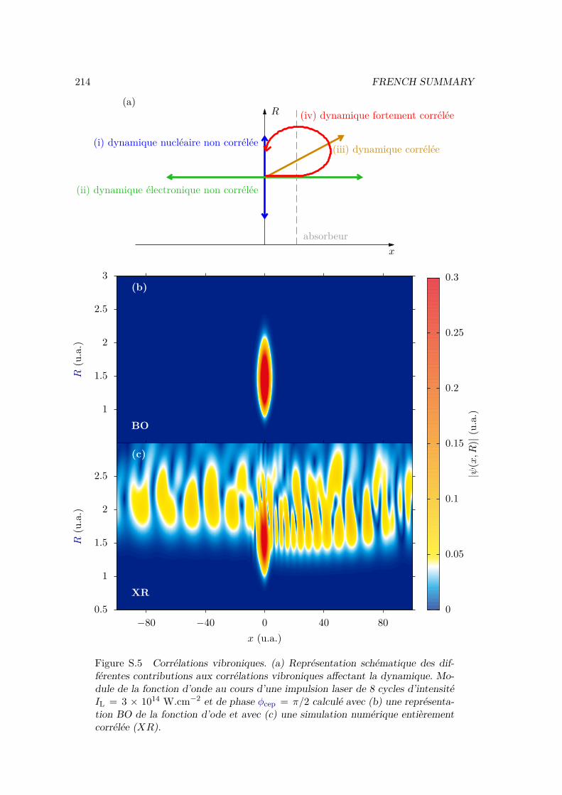
214 FRENCH SUMMARY
1
1.5
2
2.5
3
0.5
1
1.5
2
2.5
−80 −40 0 40 80
(i) dynamique nucléaire non corrélée
(ii) dynamique électronique non corrélée
(iii) dynamique corrélée
(iv) dynamique fortement corrélée
absorbeur
R(u.a.)
(b)
BO
R(u.a.)
x (u.a.)
0
0.05
0.1
0.15
0.2
0.25
0.3
|ψ(x,R
)|(u.a.)
(c)
XR
x
R(a)
Figure S.5 Corrélations vibroniques. (a) Représentation schématique des dif-férentes contributions aux corrélations vibroniques affectant la dynamique. Mo-dule de la fonction d’onde au cours d’une impulsion laser de 8 cycles d’intensitéIL = 3 × 10¹⁴ W.cm−2 et de phase φcep = π/2 calculé avec (b) une représenta-tion BO de la fonction d’ode et avec (c) une simulation numérique entièrementcorrélée (XR).
S.6 Interaction de configuration dépendante du temps 215
ne revient plus interférer avec le reste de la dynamique seront également décrites. Cescorrélations sont actuellement absentes de la fonction d’onde BO en elle-même commecela peut se voir en Figure S.5 (b) qui ne présente aucuns termes diagonaux, mais leureffet sur la dynamique nucléaire sera bien pris en compte par le modèle. Cependant, lescorrélations (iv) impliquant des termes où le paquet d’onde quitte le fondamental et re-vient influer sur la dynamique à un temps ultérieur dans l’impulsion seront complètementabsentes du modèle BO. Pour évaluer l’influence de ces corrélations j’ai comparé les ré-sultats donnés par le modèle BO avec des simulations numériques entièrement corréléesdont une fonction d’onde est montrée sur Figure S.5 (c). Ces calculs montrent que cescorrélations vibroniques influent de façon non négligeable sur le paquet d’onde vibration-nel créé, non seulement sur l’amplitude et la phase de ses oscillations, mais également surses composantes vibrationnelles. Ceci dépend de la phase du laser incident (la dénomméecarrier-envelope phase) et serait donc directement accessible expérimentalement.
S.6 Interaction de configuration dépendante du temps
Afin de pouvoir modéliser la dynamique en champ fort de systèmes plus complexes, avecplus de degrés de liberté, il est nécessaire de développer des méthodes numériques spéci-fiques. En effet, les méthodes couramment employées pour résoudre l’équation de Schrö-dinger dépendante du temps deviennent très couteuses, d’un point de vue des ressourcesnumériques, dès lors que le système possède plus d’un électron. En collaboration avec leLaboratoire de Chimie Théorique à Sorbonne Université nous avons étudié la possibilitéd’étendre les méthodes de chimie quantique, en particulier l’interaction de configuration,aux problèmes dépendants du temps. Au cours des dernières années ces méthodes ont étéoptimisées pour calculer les états liés de plusieurs types de systèmes, dont des moléculesrelativement grosses. Cependant la description des états du continuum reste encore undéfi théorique pour ces méthodes, notamment pour celles qui utilisent des fonctions debases gaussiennes. Or les états du continuum jouent un rôle central pour la modélisationde la génération d’harmoniques et pour les dynamiques électroniques en champ fort engénéral. Nous avons donc dans un premier temps analysé les performances de trois dif-férents types de fonctions de bases, grille, B-splines et gaussiennes, pour représenter cesétats du continuum et pour reproduire le spectre harmonique d’un système à un électron :H+
2 . Nous avons réalisé des simulations à une et à trois dimensions.Un spectre harmonique est présenté en Figure S.6 (b), où on voit que les trois bases
donnent des résultats très proches, tant que l’intensité du laser n’est pas trop élevée. Enparticulier le minimum d’interférence est parfaitement prédit dans les trois cas. Ceci estd’autant plus impressionnant pour les gaussiennes que cette base ne contient en tout que24 fonctions, dont seulement 5 états d’énergie positive (correspondant au "continuum")dans la gamme d’énergie concernée. Le dipôle de recombinaison est également présentéen Figure S.6 (a). Le calcul de cette grandeur suppose de calculer avec précision à la foisle fondamental et les états d’énergie positive. Dans le cas des gaussiennes, comme il n’ya que 5 états dans la gamme d’énergie considérée, on ne peut le calculer que pour ces 5valeurs. On observe néanmoins un bon accord des trois méthodes.
Le faible nombre de fonctions dans la base gaussienne est à la fois un avantage etun inconvénient. D’une part cela implique d’avoir très peu d’états d’énergie positive, et
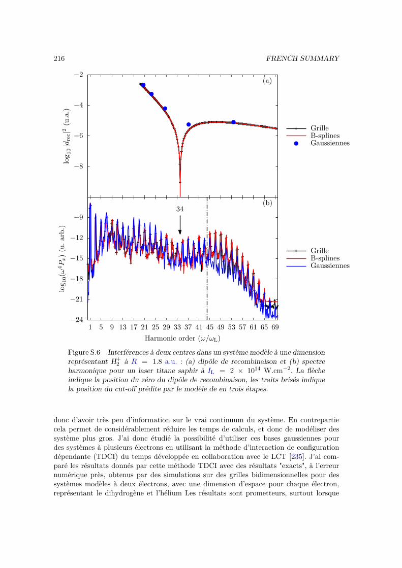
216 FRENCH SUMMARY
−8
−6
−4
−2(a)
−24
−21
−18
−15
−12
−9
1 5 9 13 17 21 25 29 33 37 41 45 49 53 57 61 65 69
(b)34
log 1
0|d
rec|2
(u.a.)
GrilleB-splinesGaussiennes
log 1
0(ω
4 Px)(u.a
rb.)
Harmonic order (ω/ωL)
GrilleB-splinesGaussiennes
Figure S.6 Interférences à deux centres dans un système modèle à une dimensionreprésentant H+
2 à R = 1.8 a.u. : (a) dipôle de recombinaison et (b) spectreharmonique pour un laser titane saphir à IL = 2 × 10¹⁴ W.cm−2. La flècheindique la position du zéro du dipôle de recombinaison, les traits brisés indiquela position du cut-off prédite par le modèle de en trois étapes.
donc d’avoir très peu d’information sur le vrai continuum du système. En contrepartiecela permet de considérablement réduire les temps de calculs, et donc de modéliser dessystème plus gros. J’ai donc étudié la possibilité d’utiliser ces bases gaussiennes pourdes systèmes à plusieurs électrons en utilisant la méthode d’interaction de configurationdépendante (TDCI) du temps développée en collaboration avec le LCT [235]. J’ai com-paré les résultats donnés par cette méthode TDCI avec des résultats "exacts", à l’erreurnumérique près, obtenus par des simulations sur des grilles bidimensionnelles pour dessystèmes modèles à deux électrons, avec une dimension d’espace pour chaque électron,représentant le dihydrogène et l’hélium Les résultats sont prometteurs, surtout lorsque
S.7 Conclusion 217
l’on utilise des bases avec des gaussiennes multi-centrées comme conseillé dans [261].
S.7 Conclusion
Au cours de ma thèse j’ai étudié différents aspects de l’interaction d’atomes et de moléculesavec des champs lasers intenses. J’ai développé des modèles analytiques pour comprendreles mécanismes derrière les processus corrélés et fortement non linéaires que l’on observeen physique des champs forts. La force de ces modèles approchés repose sur leur capacitéà construire des interprétations physiques à ces phénomènes. Pour soutenir mes interpré-tations, j’ai combiné cette approche avec les résultats de simulations numériques précisesréalisées pour des systèmes modèles. Ces systèmes simples présentent beaucoup d’avan-tages. D’un côté ils permettent de changer à volonté leurs propriétés fondamentales etdonc de se concentrer sur un ou plusieurs problèmes physiques particuliers. De plus leurdimension réduite permet de réaliser un traitement numérique approfondi. En pratiquej’ai résolu l’équation de Schrödinger dépendante du temps et l’équation de Schrödingerindépendante du temps pour extraire autant d’informations que possible de la fonctiond’onde dépendante du temps. J’ai également mis à profit ces simulations numériques pourtester les approximations sous-jacentes au modèles analytiques.
Plus précisément j’ai étudié les dynamiques électroniques et nucléaires d’atomes et demolécules diatomiques en présence d’impulsions lasers infrarouges femtosecondes. Je mesuis d’abord concentrée sur les processus électroniques fortement non linéaires qui sontdéclenchés par de telles impulsions lasers comme la génération d’harmoniques, dont j’aiétudié la première étape, c’est à dire l’ionisation tunnel, au chapitre III. Pour un laserinfrarouge, les variations temporelles du champ électrique sont très lentes comparées auxéchelles de temps électroniques. On peut donc déduire le rendement d’ionisation tunneldirectement du problème en champ statique. J’ai calculé ce rendement d’ionisation pourdifférents systèmes modèles atomiques et moléculaires. J’ai montré l’importance de l’effetStark, à la fois pour une description quantitative et qualitative de l’ionisation tunnel, etj’ai obtenu une expression analytique dans l’approximation quasi-classique qui prend ceteffet en compte. J’ai également montré que l’effet Stark représente la contribution domi-nante à l’anisotropie de l’émission tunnel pour des molécules polaires. J’ai démontré àquel point le calcul précis de l’effet Stark était important, tout particulièrement pour desmolécules très polarisables pour lesquelles la théorie des perturbations au second ordre nepermet pas d’obtenir un résultat satisfaisant. De plus, j’ai analysé les raisons à la basesdes désaccords entre formule analytique et simulations numériques. J’ai pu désintriquerles erreurs induites par les différentes approximations utilisées dans le développement ana-lytique, et j’ai trouvé que certaines approximations n’étaient en réalité pas justifiées, maisqu’une compensation d’erreur permettant d’obtenir néanmoins des résultats raisonnables.
Une des applications directes de la physique des champs fort est la spectroscopie dehautes harmoniques (HHS), où la lumière émise par la génération d’harmoniques est ana-lysée pour extraire des informations structurelles et dynamiques sur le système émetteur.Dans le cas particulier des interférences à deux centres dans des molécules diatomiqueshomonucléaires j’ai cherché à comprendre, au chapitre IV, les conditions dans lesquellescet interférences pouvaient présenter le meilleur contraste, et donc être plus facilementmesurables expérimentalement. J’ai complété le développement analytique réalisé pour
218 FRENCH SUMMARY
des molécules alignées avec le laser [129]. Je lui ai donné un fondement plus rigoureuxen définissant un paramètre, i.e. la distance internucléaire R, pour le développement detype Taylor du SFA moléculaire. J’ai aussi obtenu l’expression complète du spectre har-monique au premier ordre de ce développement et je l’ai étendu au cas d’une orientationquelconque de la molécule et du champ électrique. J’ai évalué les prédictions de ce modèleanalytique en les confrontant à des simulations numériques pour différents systèmes. Encomparant les résultats obtenus à une et à deux dimensions, j’ai conclu que l’étalementtransverse du paquet d’onde électronique au cours de la propagation après l’ionisation tun-nel avait en réalité un impact sur les interférences à deux centres. Finalement, j’ai réaliséune analyse détaillée de l’erreur induite par les deux approximations sous-jacentes au SFAmoléculaire : la LCAO et la PWA. J’ai démontré que chacune de ces deux approximationsinduisait en réalité des erreurs non négligeables mais qui ont la chance de se compenser,ce qui permet au SFA moléculaire de prédire la position du minimum d’interférence avecune précision raisonnable.
Pour des molécules très légères comme H2 l’approximation qui consiste à geler lesdegrés de liberté nucléaires n’est en réalité pas valable, même pour des impulsions trèscourtes de quelques femtosecondes. Au chapitre V, j’ai étudié les couplages entre degrésde liberté électroniques et nucléaires pour des systèmes modèles représentant des mo-lécules diatomiques homonucléaires. J’ai évalué la capacité du modèle BO à modéliserces couplages à travers l’introduction d’un rendement d’ionisation et d’un effet Stark dé-pendant de la distance internucléaire R. J’ai montré la nécessité de considérer les deuxmécanismes du Lochfraß et du Bond-Softening comme un tout cohérent, et non commedeux mécanismes indépendants et décorrélés comme cela est souvent fait [222, 223, 227].J’ai également trouvé des conditions pour pouvoir observer expérimentalement l’effet decouplages vibroniques sur la dynamique nucléaire qui ne sont pas pris en compte par cemodèle de BO, et qui vont donc plus loin que ce qui peut être décrit par le Lochfraßet le Bond-Softening. Finalement, j’ai proposé un modèle analytique basé sur l’approcheWigner-Weisskopf pour donner un cadre plus rigoureux au mécanisme du Bond-Softening.Cela m’a permis d’obtenir un terme correctif qui pourrait tenir compte d’une partie descorrélations négligées par le modèle de BO, mais qui reste à évaluer. Ce modèle pourraitêtre étendu au cas du Lochfraß, mais cela reste à faire.
Dans un dernier chapitre, j’ai étudié différentes méthodes numériques pour résoudre laTDSE de systèmes plus gros et plus complexes pour lesquels les corrélations électroniquesjouent un rôle dans la dynamique en champ fort. En collaboration avec le LCT, nousavons étudié trois différentes bases pour représenter la fonction d’onde dépendante dutemps. Nous avons montré que les grilles et les B-splines étaient toutes deux capables dereproduire efficacement la dynamique électronique de H+
2 tant à une qu’à trois dimensions.Cependant les ressources numériques importantes qu’elles nécessitent les rendent difficilesà envisager pour de plus gros systèmes. Nous avons trouvé que les gaussiennes étaient enréalité capables, tant que l’intensité du laser n’est pas trop élevée, de reproduire le spectreharmonique de H+
2 , y compris des effets fins tels que les interférences à deux centreset les résonances de types hyper-Raman. Ceci était d’autant plus inattendu qu’elle nepermettent d’obtenir que quelques états d’énergie positive, ce qui les empêche de décrirecorrectement des phénomènes tels que l’ionisation au dessus du seuil. En mettant à profitles faibles ressources numériques nécessaires au gaussiennes, nous avons développé unTDCI basées sur des gaussiennes, pour résoudre la TDSE de systèmes poly-électroniques.

S.7 Conclusion 219
J’ai testé les performances de cette méthode en la comparant à des simulations numériques"exactes", à l’erreur numérique près, réalisées sur des grilles bidimensionnelles. J’ai trouvéque cette méthode était prometteuse pour le calcul de spectres harmonique de grossesmolécules.
La complète compréhension des phénomènes physiques en champs fort n’est pas pourdemain. J’espère avoir réussi à montrer que des petits modèles simples, combinés à desraisonnements analytiques approchés, pouvaient apporter une aide précieuse dans ce do-maine. Personne ne peut savoir d’où viendront les prochaines idées révolutionnaires, maisje suis convaincue que ces systèmes modèles intuitifs aident en tout cas à alimenter notreimagination de physiciens.

220 FRENCH SUMMARY

Bibliography
[1] P. Mulser & D. Bauer. High power laser-matter interaction. No. 238 in Springertracts in modern physics (Springer, Heidelberg) (2010). OCLC: 699733993. 1, 205
[2] D. Strickland & G. Mourou. Compression of amplified chirped optical pulses.Optics Communications 56, 219 (1985). URL http://dx.doi.org/10.1016/0030-4018(85)90120-8. 1, 205
[3] A. H. Zewail. Laser Femtochemistry. Science 242, 1645 (1988). URL http://dx.doi.org/10.1126/science.242.4886.1645. 1, 205
[4] A. H. Zewail. Femtochemistry: Atomic-Scale Dynamics of the Chemical Bond. J.Phys. Chem. A 104, 5660 (2000). URL http://dx.doi.org/10.1021/jp001460h.1, 205
[5] P. Agostini, F. Fabre, G. Mainfray, G. Petite & N. K. Rahman. Free-FreeTransitions Following Six-Photon Ionization of Xenon Atoms. Physical Review Let-ters 42, 1127 (1979). URL http://dx.doi.org/10.1103/PhysRevLett.42.1127.1, 205
[6] A. L’Huillier, L. A. Lompre, G. Mainfray & C. Manus. Multiply ChargedIons Formed by Multiphoton Absorption Processes in the Continuum. Phys. Rev.Lett. 48, 1814 (1982). URL http://dx.doi.org/10.1103/PhysRevLett.48.1814.1, 205
[7] A. McPherson, G. Gibson, H. Jara, U. Johann, T. S. Luk, I. A. McIntyre,K. Boyer & C. K. Rhodes. Studies of multiphoton production of vacuum-ultraviolet radiation in the rare gases. J. Opt. Soc. Am. B, JOSAB 4, 595 (1987).URL http://dx.doi.org/10.1364/JOSAB.4.000595. 1, 21, 206
[8] M. Ferray, A. L’Huillier, X. F. Li, L. A. Lompre, G. Mainfray &C. Manus. Multiple-harmonic conversion of 1064 nm radiation in rare gases. J.Phys. B: At. Mol. Opt. Phys. 21, L31 (1988). URL http://dx.doi.org/10.1088/0953-4075/21/3/001. 1, 21, 206
[9] M. Y. Kuchiev. Atomic antenna. JETP Lett. 45, 404 (1987). URL http://www.jetpletters.ac.ru/ps/1241/article_18763.shtml. 1, 26, 75, 206, 209
[10] J. L. Krause, K. J. Schafer & K. C. Kulander. High-order harmonic genera-tion from atoms and ions in the high intensity regime. Physical Review Letters 68,
221

222 BIBLIOGRAPHY
3535 (1992). URL http://dx.doi.org/10.1103/PhysRevLett.68.3535. 26, 150,209
[11] M. Lewenstein, P. Balcou, M. Y. Ivanov, A. L’huillier & P. B. Corkum.Theory of high-harmonic generation by low-frequency laser fields. Phys. Rev.A 49, 2117 (1994). URL http://journals.aps.org/pra/abstract/10.1103/PhysRevA.49.2117. 1, 21, 32, 34, 36, 66, 75, 154, 158, 159, 206, 209
[12] M. Hentschel, R. Kienberger, C. Spielmann, G. A. Reider, N. Milosevic,T. Brabec, P. Corkum, U. Heinzmann, M. Drescher & F. Krausz. At-tosecond metrology. Nature 414, 509 (2001). URL http://dx.doi.org/10.1038/35107000. 1, 5, 67, 206
[13] R. López-Martens et al. Amplitude and Phase Control of Attosecond LightPulses. Physical Review Letters 94 (2005). URL http://dx.doi.org/10.1103/PhysRevLett.94.033001.
[14] D. H. Ko, K. T. Kim, J. Park, J.-h. Lee & C. H. Nam. Attosecond chirpcompensation over broadband high-order harmonics to generate near transform-limited 63 as pulses. New J. Phys. 12, 063008 (2010). URL http://dx.doi.org/10.1088/1367-2630/12/6/063008. 1, 206
[15] T. Gaumnitz, A. Jain, Y. Pertot, M. Huppert, I. Jordan, F. Ardana-Lamas & H. J. Wörner. Streaking of 43-attosecond soft-X-ray pulses generatedby a passively CEP-stable mid-infrared driver. Opt. Express, OE 25, 27506 (2017).URL http://dx.doi.org/10.1364/OE.25.027506. 1, 206
[16] A. Scrinzi, M. Y. Ivanov, R. Kienberger & D. M. Villeneuve. Attosecondphysics. J. Phys. B: At. Mol. Opt. Phys. 39, R1 (2006). URL http://dx.doi.org/10.1088/0953-4075/39/1/R01. 2, 206
[17] P. B. Corkum & F. Krausz. Attosecond science. Nature Physics 3, 381 (2007).URL http://dx.doi.org/10.1038/nphys620.
[18] F. Calegari, G. Sansone, S. Stagira, C. Vozzi & M. Nisoli. Advances inattosecond science. J. Phys. B: At. Mol. Opt. Phys. 49, 062001 (2016). URLhttp://dx.doi.org/10.1088/0953-4075/49/6/062001.
[19] F. Krausz. The birth of attosecond physics and its coming of age. Phys. Scr. 91,063011 (2016). URL http://dx.doi.org/10.1088/0031-8949/91/6/063011. 2,206
[20] M. Schultze et al. Delay in Photoemission. Science 328, 1658 (2010). URLhttp://dx.doi.org/10.1126/science.1189401. 2, 206
[21] K. Klünder et al. Probing Single-Photon Ionization on the Attosecond TimeScale. Physical Review Letters 106 (2011). URL http://dx.doi.org/10.1103/PhysRevLett.106.143002. 2, 206

BIBLIOGRAPHY 223
[22] S. Beaulieu et al. Attosecond-resolved photoionization of chiral molecules. Science358, 1288 (2017). URL http://dx.doi.org/10.1126/science.aao5624. 2, 20,206
[23] A. L. Cavalieri et al. Attosecond spectroscopy in condensed matter. Nature 449,1029 (2007). URL http://dx.doi.org/10.1038/nature06229. 2, 206
[24] S. Neppl, R. Ernstorfer, E. M. Bothschafter, A. L. Cavalieri, D. Men-zel, J. V. Barth, F. Krausz, R. Kienberger & P. Feulner. AttosecondTime-Resolved Photoemission from Core and Valence States of Magnesium. Physi-cal Review Letters 109 (2012). URL http://dx.doi.org/10.1103/PhysRevLett.109.087401. 2, 206
[25] M. Drescher, M. Hentschel, R. Kienberger, M. Uiberacker, V. Yakovlev,A. Scrinzi, T. Westerwalbesloh, U. Kleineberg, U. Heinzmann &F. Krausz. Time-resolved atomic inner-shell spectroscopy. Nature 419, 803 (2002).URL http://dx.doi.org/10.1038/nature01143. 2, 206
[26] M. Uiberacker et al. Attosecond real-time observation of electron tunnelling inatoms. Nature 446, 627 (2007). URL http://dx.doi.org/10.1038/nature05648.2, 206
[27] D. M. Villeneuve, P. Hockett, M. J. J. Vrakking & H. Niikura. Coherentimaging of an attosecond electron wave packet. Science 356, 1150 (2017). URLhttp://dx.doi.org/10.1126/science.aam8393. 2, 20, 206
[28] F. Calegari et al. Ultrafast electron dynamics in phenylalanine initiated by at-tosecond pulses. Science 346, 336 (2014). URL http://dx.doi.org/10.1126/science.1254061. 2, 206
[29] M. Schultze et al. Attosecond band-gap dynamics in silicon. Science 346, 1348(2014). URL http://dx.doi.org/10.1126/science.1260311. 2, 20, 30, 206
[30] S. Neppl et al. Direct observation of electron propagation and dielectric screeningon the atomic length scale. Nature 517, 342 (2015). URL http://dx.doi.org/10.1038/nature14094.
[31] C. Lemell, S. Neppl, G. Wachter, K. Tőkési, R. Ernstorfer, P. Feulner,R. Kienberger & J. Burgdörfer. Real-time observation of collective excitationsin photoemission. Physical Review B 91 (2015). URL http://dx.doi.org/10.1103/PhysRevB.91.241101. 2, 206
[32] V. Gruson et al. Attosecond dynamics through a fano resonance: Monitoringthe birth of a photoelectron. Science 354, 734 (2016). URL http://science.sciencemag.org/content/354/6313/734.abstract. 2, 5, 20, 67, 206
[33] A. Kaldun et al. Observing the ultrafast buildup of a Fano resonance in the timedomain. Science 354, 738 (2016). URL http://dx.doi.org/10.1126/science.aah6972. 2, 20, 206

224 BIBLIOGRAPHY
[34] A. S. Alnaser et al. Subfemtosecond steering of hydrocarbon deprotonationthrough superposition of vibrational modes. Nature Communications 5, 3800(2014). URL http://dx.doi.org/10.1038/ncomms4800. 2, 206
[35] P. Hommelhoff & M. F. Kling. Attosecond Nanophysics: From Basic Scienceto Applications (Wiley-VCH) (2015). 2, 206
[36] M. F. Ciappina et al. Attosecond physics at the nanoscale. Rep. Prog. Phys. 80,054401 (2017). URL http://dx.doi.org/10.1088/1361-6633/aa574e.
[37] M. I. Stockman et al. Roadmap on plasmonics. J. Opt. 20, 043001 (2018). URLhttp://dx.doi.org/10.1088/2040-8986/aaa114. 2, 206
[38] F. Süßmann et al. Field propagation-induced directionality of carrier-envelopephase-controlled photoemission from nanospheres. Nature Communications 6, 7944(2015). URL http://dx.doi.org/10.1038/ncomms8944. 2, 206
[39] B. Förg et al. Attosecond nanoscale near-field sampling. Nature Communications7, 11717 (2016). URL http://dx.doi.org/10.1038/ncomms11717.
[40] L. Seiffert et al. Attosecond chronoscopy of electron scattering in dielectricnanoparticles. Nature Physics 13, 766 (2017). URL http://dx.doi.org/10.1038/nphys4129. 2, 206
[41] S. Haessler, J. Caillat & P. Salières. Self-probing of molecules with highharmonic generation. J. Phys. B: At. Mol. Opt. Phys. 44, 203001 (2011). URLhttp://dx.doi.org/10.1088/0953-4075/44/20/203001. 2, 20, 206
[42] M. Lein. Attosecond Probing of Vibrational Dynamics with High-Harmonic Gen-eration. Physical Review Letters 94 (2005). URL http://dx.doi.org/10.1103/PhysRevLett.94.053004. 2, 206
[43] S. Baker, J. S. Robinson, C. A. Haworth, H. Teng, R. A. Smith, C. C.Chirilă, M. Lein, J. W. G. Tisch & J. P. Marangos. Probing Proton Dynamicsin Molecules on an Attosecond Time Scale. Science 312, 424 (2006). URL http://dx.doi.org/10.1126/science.1123904.
[44] S. Baker et al. Dynamic Two-Center Interference in High-Order Harmonic Gen-eration from Molecules with Attosecond Nuclear Motion. Phys. Rev. Lett. 101,053901 (2008). URL http://dx.doi.org/10.1103/PhysRevLett.101.053901. 2,206
[45] S. Haessler et al. Attosecond imaging of molecular electronic wavepackets. Nat.Phys. 6, 200 (2010). URL http://dx.doi.org/10.1038/nphys1511. 2, 20, 206
[46] J. Itatani, J. Levesque, D. Zeidler, H. Niikura, H. Pépin, J. C. Kieffer,P. B. Corkum & D. M. Villeneuve. Tomographic imaging of molecular orbitals.Nature 432, 867 (2004). URL http://dx.doi.org/10.1038/nature03183. 2, 164,206
BIBLIOGRAPHY 225
[47] C. Vozzi, M. Negro, F. Calegari, G. Sansone, M. Nisoli, S. D. Silvestri& S. Stagira. Generalized molecular orbital tomography. Nature Physics 7, 822(2011). URL http://dx.doi.org/10.1038/nphys2029.
[48] P. Salières, A. Maquet, S. Haessler, J. Caillat & R. Taïeb. Imaging orbitalswith attosecond and Ångström resolutions: toward attochemistry? Rep. Prog. Phys.75, 062401 (2012). URL http://dx.doi.org/10.1088/0034-4885/75/6/062401.2, 206
[49] A. D. Shiner, B. E. Schmidt, C. Trallero-Herrero, H. J. Wörner,S. Patchkovskii, P. B. Corkum, J.-C. Kieffer, F. Légaré & D. M. Vil-leneuve. Probing collective multi-electron dynamics in xenon with high-harmonicspectroscopy. Nature Physics 7, 464 (2011). URL http://dx.doi.org/10.1038/nphys1940. 2, 149, 206
[50] O. Smirnova, Y. Mairesse, S. Patchkovskii, N. Dudovich, D. Villeneuve,P. Corkum & M. Y. Ivanov. High harmonic interferometry of multi-electrondynamics in molecules. Nature 460, 972 (2009). URL http://dx.doi.org/10.1038/nature08253. 2, 5, 20, 150, 164, 206
[51] R. E. F. Silva, I. V. Blinov, A. N. Rubtsov, O. Smirnova & M. Ivanov.High-harmonic spectroscopy of ultrafast many-body dynamics in strongly correlatedsystems. Nature Photonics 12, 266 (2018). URL http://dx.doi.org/10.1038/s41566-018-0129-0. 2, 206
[52] O. Smirnova, Y. Mairesse & S. Patchkovskii. Opportunities for chiral discrim-ination using high harmonic generation in tailored laser fields. J. Phys. B: At. Mol.Opt. Phys. 48, 234005 (2015). URL http://dx.doi.org/10.1088/0953-4075/48/23/234005. 2
[53] D. Ayuso, P. Decleva, S. Patchkovskii & O. Smirnova. Chiral dichroism inbi-elliptical high-order harmonic generation. J. Phys. B: At. Mol. Opt. Phys. 51,06LT01 (2018). URL http://dx.doi.org/10.1088/1361-6455/aaae5e.
[54] D. Ayuso, P. Decleva, S. Patchkovskii & O. Smirnova. Strong-field controland enhancement of chiral response in bi-elliptical high-order harmonic generation:an analytical model. J. Phys. B: At. Mol. Opt. Phys. 51, 124002 (2018). URLhttp://dx.doi.org/10.1088/1361-6455/aabc95. 2
[55] R. Cireasa et al. Probing molecular chirality on a sub-femtosecond timescale.Nature Physics 11, 654 (2015). URL http://dx.doi.org/10.1038/nphys3369. 2,206
[56] D. Baykusheva, M. S. Ahsan, N. Lin & H. J. Wörner. Bicircu-lar High-Harmonic Spectroscopy Reveals Dynamical Symmetries of Atoms andMolecules. Physical Review Letters 116 (2016). URL http://dx.doi.org/10.1103/PhysRevLett.116.123001. 2, 206
226 BIBLIOGRAPHY
[57] S. Choi & B. Sundaram. Bose-Einstein condensate as a nonlinear Ramsey in-terferometer operating beyond the Heisenberg limit. Physical Review A 77 (2008).URL http://dx.doi.org/10.1103/PhysRevA.77.053613. 5
[58] A. Widera, O. Mandel, M. Greiner, S. Kreim, T. W. Hänsch & I. Bloch.Entanglement Interferometry for Precision Measurement of Atomic Scattering Prop-erties. Physical Review Letters 92 (2004). URL http://dx.doi.org/10.1103/PhysRevLett.92.160406. 5
[59] C. D. Lin, A.-T. Le, Z. Chen, T. Morishita & R. Lucchese. Strong-fieldrescattering physics—self-imaging of a molecule by its own electrons. J. Phys.B: At. Mol. Opt. Phys. 43, 122001 (2010). URL http://dx.doi.org/10.1088/0953-4075/43/12/122001. 5, 20, 75
[60] C. Zhai, X. Zhu, P. Lan, F. Wang, L. He, W. Shi, Y. Li, M. Li, Q. Zhang& P. Lu. Diffractive molecular-orbital tomography. Phys. Rev. A 95, 033420(2017). URL http://dx.doi.org/10.1103/PhysRevA.95.033420. 5
[61] M. Vacher, R. Gaillac, A. Maquet, R. Taïeb & J. Caillat. Transitiondynamics in two-photon ionisation. Journal of Optics 19, 114011 (2017). URLhttp://dx.doi.org/10.1088/2040-8986/aa8f56. 5
[62] Y.-L. Cao et al. MFN1 structures reveal nucleotide-triggered dimerization criticalfor mitochondrial fusion. Nature 542, 372 (2017). URL http://dx.doi.org/10.1038/nature21077. 5
[63] Y. Yuan et al. Cryo-EM structures of MERS-CoV and SARS-CoV spike glyco-proteins reveal the dynamic receptor binding domains. Nature Comm. 8, 15092(2017). URL http://dx.doi.org/10.1038/ncomms15092.
[64] H. N. Chapman et al. Femtosecond diffractive imaging with a soft-X-ray free-electron laser. Nature Phys. 2, 839 (2006). URL http://dx.doi.org/10.1038/nphys461.
[65] J. Kern et al. Simultaneous Femtosecond X-ray Spectroscopy and Diffractionof Photosystem II at Room Temperature. Science 340, 491 (2013). URL http://dx.doi.org/10.1126/science.1234273.
[66] T. Ekeberg et al. Three-Dimensional Reconstruction of the Giant MimivirusParticle with an X-Ray Free-Electron Laser. Phys. Rev. Lett. 114 (2015). URLhttp://dx.doi.org/10.1103/PhysRevLett.114.098102. 5
[67] A. Ashkin. Acceleration and trapping of particles by radiation pressure. Physicalreview letters 24, 156 (1970). 5
[68] S. Bennetts, C.-C. Chen, B. Pasquiou & F. Schreck. Steady-State Magneto-Optical Trap with 100-Fold Improved Phase-Space Density. Phys. Rev. Lett. 119(2017). URL http://dx.doi.org/10.1103/PhysRevLett.119.223202. 5
[69] D. Meschede, T. Udem & T. Esslinger. Exploring the World with the Laser(Springer) (2018). 5
BIBLIOGRAPHY 227
[70] T. Peyronel, O. Firstenberg, Q.-Y. Liang, S. Hofferberth, A. V. Gor-shkov, T. Pohl, M. D. Lukin & V. Vuletić. Quantum nonlinear optics withsingle photons enabled by strongly interacting atoms. Nature 488, 57 (2012). URLhttp://dx.doi.org/10.1038/nature11361. 5
[71] C. Sayrin et al. Real-time quantum feedback prepares and stabilizes photonnumber states. Nature 477, 73 (2011). URL http://dx.doi.org/10.1038/nature10376. 5
[72] M. M. Kash, V. A. Sautenkov, A. S. Zibrov, L. Hollberg, G. R. Welch,M. D. Lukin, Y. Rostovtsev, E. S. Fry & M. O. Scully. Ultraslow groupvelocity and enhanced nonlinear optical effects in a coherently driven hot atomicgas. Physical Review Letters 82, 5229 (1999). 5
[73] D. F. Phillips, A. Fleischhauer, A. Mair, R. L. Walsworth & M. D. Lukin.Storage of Light in Atomic Vapor. Physical Review Letters 86, 783 (2001). URLhttp://dx.doi.org/10.1103/PhysRevLett.86.783.
[74] P. Vernaz-Gris, K. Huang, M. Cao, A. S. Sheremet & J. Laurat. Highly-efficient quantum memory for polarization qubits in a spatially-multiplexed coldatomic ensemble. Nature Communications 9, 363 (2018). URL http://dx.doi.org/10.1038/s41467-017-02775-8. 5
[75] H. G. Muller. Reconstruction of attosecond harmonic beating by interference oftwo-photon transitions. Appl Phys B 74, s17 (2002). URL http://dx.doi.org/10.1007/s00340-002-0894-8. 5
[76] Y. Mairesse & F. Quéré. Frequency-resolved optical gating for complete re-construction of attosecond bursts. Physical Review A 71 (2005). URL http://dx.doi.org/10.1103/PhysRevA.71.011401.
[77] V. S. Yakovlev, F. Bammer & A. Scrinzi. Attosecond streaking measurements.Journal of Modern Optics 52, 395 (2005). URL http://dx.doi.org/10.1080/09500340412331283642. 5
[78] J.-M. Raimond. Atoms and photons. http://www.lkb.upmc.fr/cqed/teaching/teachingjmr/ (2016). 6, 62, 142
[79] J. D. Jackson. Classical Electrodynamics (John Wiley & Sons, Inc.), third edn.(1998). 7
[80] E. Cormier & P. Lambropoulos. Optimal gauge and gauge invariance in non-perturbative time-dependent calculation of above-threshold ionization. J. Phys.B: At. Mol. Opt. Phys. 29, 1667 (1996). URL http://dx.doi.org/10.1088/0953-4075/29/9/013. 10
[81] M. Baghery, U. Saalmann & J. M. Rost. Essential Conditions for DynamicInterference. Physical Review Letters 118 (2017). URL http://dx.doi.org/10.1103/PhysRevLett.118.143202. 10
228 BIBLIOGRAPHY
[82] K. J. Schafer & K. C. Kulander. Energy analysis of time-dependent wavefunctions: Application to above-threshold ionization. Phys. Rev. A 42, 5794 (1990).URL http://dx.doi.org/10.1103/PhysRevA.42.5794. 11, 68, 71
[83] J. Crank, P. Nicolson & D. R. Hartree. A practical method for numeri-cal evaluation of solutions of partial differential equations of the heat-conductiontype. Math. Proc. Cambridge 43, 50 (1947). URL http://dx.doi.org/10.1017/S0305004100023197. 11, 47, 152, 153
[84] C. C. Chirilă & M. Lein. Strong-field approximation for harmonic generation indiatomic molecules. Phys. Rev. A 73, 023410 (2006). URL http://dx.doi.org/10.1103/PhysRevA.73.023410. 12, 35, 37, 39, 98, 117, 120, 164
[85] A. Galstyan, O. Chuluunbaatar, A. Hamido, Y. V. Popov, F. Mota-Furtado, P. F. O’Mahony, N. Janssens, F. Catoire & B. Piraux. Refor-mulation of the strong-field approximation for light-matter interactions. PhysicalReview A 93 (2016). URL http://dx.doi.org/10.1103/PhysRevA.93.023422. 12
[86] C. Cohen-Tannoudji, B. Diu & F. Laloë. Mécanique quantique, vol. 2 (Her-mann) (1973). 12, 208
[87] K. W. D. Ledingham & R. P. Singhal. High intensity laser mass spectrometry— a review. International Journal of Mass Spectrometry and Ion Processes 163,149 (1997). URL http://dx.doi.org/10.1016/S0168-1176(97)00015-3. 17
[88] K. Kimura. Development of laser photoelectron spectroscopy based on resonantlyenhanced multiphoton ionization. Journal of Electron Spectroscopy and RelatedPhenomena 100, 273 (1999). URL http://dx.doi.org/10.1016/S0368-2048(99)00051-1.
[89] K. Kimura. Very-High-Resolution Laser Photoelectron Spectroscopy of Molecules.In Very High Resolution Photoelectron Spectroscopy, Lecture Notes in Physics, pp.215–239 (Springer, Berlin, Heidelberg) (2007). URL http://dx.doi.org/10.1007/3-540-68133-7_8. 17
[90] P. Salières, A. L’Huillier & M. Lewenstein. Coherence Control of High-OrderHarmonics. Phys. Rev. Lett. 74, 3776 (1995). URL http://dx.doi.org/10.1103/PhysRevLett.74.3776. 20, 21, 30
[91] P. B. Corkum. Plasma perspective on strong field multiphoton ionization. Phys.Rev. Lett. 71, 1994 (1993). URL http://dx.doi.org/10.1103/PhysRevLett.71.1994. 20, 26, 30, 75, 154, 158, 159, 209
[92] K. J. Schafer, B. Yang, L. F. DiMauro & K. C. Kulander. Above thresh-old ionization beyond the high harmonic cutoff. Physical Review Letters 70, 1599(1993). URL http://dx.doi.org/10.1103/PhysRevLett.70.1599. 20, 26
[93] D. B. Milošević, G. G. Paulus, D. Bauer & W. Becker. Above-thresholdionization by few-cycle pulses. J. Phys. B: At. Mol. Opt. Phys. 39, R203 (2006).URL http://dx.doi.org/10.1088/0953-4075/39/14/R01. 20

BIBLIOGRAPHY 229
[94] A. Becker, R. Dörner & R. Moshammer. Multiple fragmentation of atoms infemtosecond laser pulses. J. Phys. B: At. Mol. Opt. Phys. 38, S753 (2005). URLhttp://dx.doi.org/10.1088/0953-4075/38/9/021. 20, 75
[95] P. Antoine, A. L’Huillier & M. Lewenstein. Attosecond Pulse Trains UsingHigh–Order Harmonics. Phys. Rev. Lett. 77, 1234 (1996). URL http://dx.doi.org/10.1103/PhysRevLett.77.1234. 20, 21, 65
[96] P. Salières, A. L’Huillier, P. Antoine & M. Lewenstein. Study of the spatialand temporal coherence of high order harmonics. arXiv:quant-ph/9710060 (1997).URL http://arxiv.org/abs/quant-ph/9710060. ArXiv: quant-ph/9710060. 21,30, 65, 75
[97] Y. Mairesse. Attosecond Synchronization of High-Harmonic Soft X-rays. Science302, 1540 (2003). URL http://dx.doi.org/10.1126/science.1090277. 20
[98] P. M. Kraus, A. Rupenyan & H. J. Wörner. High-Harmonic Spectroscopy ofOriented OCS Molecules: Emission of Even and Odd Harmonics. Phys. Rev. Lett.109 (2012). URL http://dx.doi.org/10.1103/PhysRevLett.109.233903. 20, 32
[99] A. Rupenyan, P. Kraus, J. Schneider & H. Wörner. High-harmonic spec-troscopy of isoelectronic molecules: Wavelength scaling of electronic-structure andmultielectron effects. Phys. Rev. A 87 (2013). URL http://dx.doi.org/10.1103/PhysRevA.87.033409. 20, 76, 77, 97, 212
[100] S. Ghimire, A. D. DiChiara, E. Sistrunk, P. Agostini, L. F. DiMauro& D. A. Reis. Observation of high-order harmonic generation in a bulk crystal.Nature Physics 7, 138 (2011). URL http://dx.doi.org/10.1038/nphys1847. 21
[101] S. Ghimire, G. Ndabashimiye, A. D. DiChiara, E. Sistrunk, M. I. Stock-man, Pierre Agostini, L. F. DiMauro & D. A. Reis. Strong-field and at-tosecond physics in solids. J. Phys. B: At. Mol. Opt. Phys. 47, 204030 (2014). URLhttp://dx.doi.org/10.1088/0953-4075/47/20/204030.
[102] G. Ndabashimiye, S. Ghimire, M. Wu, D. A. Browne, K. J. Schafer,M. B. Gaarde & D. A. Reis. Solid-state harmonics beyond the atomic limit.Nature 534, 520 (2016). URL http://dx.doi.org/10.1038/nature17660. 21
[103] M. Sivis, M. Taucer, G. Vampa, K. Johnston, A. Staudte, A. Y. Naumov,D. M. Villeneuve, C. Ropers & P. B. Corkum. Tailored semiconductors forhigh-harmonic optoelectronics. Science 357, 303 (2017). URL http://dx.doi.org/10.1126/science.aan2395. 21
[104] G. Vampa et al. Plasmon-enhanced high-harmonic generation from silicon. NaturePhysics 13, 659 (2017). URL http://dx.doi.org/10.1038/nphys4087. 21
[105] A. D. DiChiara, E. Sistrunk, T. A. Miller, P. Agostini & L. F. DiMauro.An investigation of harmonic generation in liquid media with a mid-infrared laser.Opt. Express, OE 17, 20959 (2009). URL http://dx.doi.org/10.1364/OE.17.020959. 21

230 BIBLIOGRAPHY
[106] A. L’Huillier, K. J. Schafer & K. C. Kulander. Theoretical aspects of intensefield harmonic generation. J. Phys. B: At. Mol. Opt. Phys. 24, 3315 (1991). URLhttp://dx.doi.org/10.1088/0953-4075/24/15/004. 21, 30
[107] I. P. Christov, M. M. Murnane & H. C. Kapteyn. Generation and propa-gation of attosecond x-ray pulses in gaseous media. Physical Review A 57, R2285(1998). URL http://dx.doi.org/10.1103/PhysRevA.57.R2285. 21
[108] M. B. Gaarde, J. L. Tate & K. J. Schafer. Macroscopic aspects of attosecondpulse generation. J. Phys. B: At. Mol. Opt. Phys. 41, 132001 (2008). URL http://dx.doi.org/10.1088/0953-4075/41/13/132001. 21, 30
[109] X. F. Li, A. L’Huillier, M. Ferray, L. A. Lompre & G. Mainfray. Multiple-harmonic generation in rare gases at high laser intensity. Physical Review A 39,5751 (1989). URL http://dx.doi.org/10.1103/PhysRevA.39.5751. 21
[110] G. Farkas & C. Tóth. Proposal for attosecond light pulse generation using laserinduced multiple-harmonic conversion processes in rare gases. Physics Letters A168, 447 (1992). URL http://dx.doi.org/10.1016/0375-9601(92)90534-S.
[111] J. J. Macklin, J. D. Kmetec & C. L. Gordon. High-order harmonic generationusing intense femtosecond pulses. Physical Review Letters 70, 766 (1993). URLhttp://dx.doi.org/10.1103/PhysRevLett.70.766. 21
[112] P. M. Paul, E. S. Toma, P. Breger, G. Mullot, F. Augé, P. Balcou, H. G.Muller & P. Agostini. Observation of a Train of Attosecond Pulses from HighHarmonic Generation. Science 292, 1689 (2001). URL http://dx.doi.org/10.1126/science.1059413. 21, 67
[113] L. V. Keldysh. Ionization in the field of a strong electromagnetic wave. Sov. Phys.JETP 20, 1307 (1965). URL http://jetp.ac.ru/cgi-bin/dn/e_020_05_1307.pdf. 21, 75, 207, 210
[114] M. V. Frolov, N. L. Manakov, A. M. Popov, O. V. Tikhonova, E. A.Volkova, A. A. Silaev, N. V. Vvedenskii & A. F. Starace. Analytic theoryof high-order-harmonic generation by an intense few-cycle laser pulse. PhysicalReview A 85 (2012). URL http://dx.doi.org/10.1103/PhysRevA.85.033416.24, 142
[115] M. Y. Ivanov, T. Brabec & N. Burnett. Coulomb corrections and polarizationeffects in high-intensity high-harmonic emission. Physical Review A 54, 742 (1996).URL http://dx.doi.org/10.1103/PhysRevA.54.742. 28
[116] M. B. Gaarde, F. Salin, E. Constant, P. Balcou, K. J. Schafer, K. C.Kulander & A. L’Huillier. Spatiotemporal separation of high harmonic radiationinto two quantum path components. Phys. Rev. A 59, 1367 (1999). URL https://journals.aps.org/pra/abstract/10.1103/PhysRevA.59.1367. 30
[117] M. Bellini, C. Lyngtextbackslasha a, A. Tozzi, M. B. Gaarde, T. W.Hänsch, A. L’Huillier & C.-G. Wahlström. Temporal coherence of ultrashorthigh-order harmonic pulses. Phys. Rev. Lett. 81, 297 (1998). 30
BIBLIOGRAPHY 231
[118] L. Medišauskas, J. Wragg, H. van der Hart & M. Y. Ivanov. GeneratingIsolated Elliptically Polarized Attosecond Pulses Using Bichromatic Counterrotat-ing Circularly Polarized Laser Fields. Physical Review Letters 115 (2015). URLhttp://dx.doi.org/10.1103/PhysRevLett.115.153001. 32
[119] C. A. Mancuso et al. Strong-field ionization with two-color circularly polarizedlaser fields. Physical Review A 91 (2015). URL http://dx.doi.org/10.1103/PhysRevA.91.031402.
[120] D. B. Milošević. High-order harmonic generation by a bichromatic ellipticallypolarized field: conservation of angular momentum. J. Phys. B: At. Mol. Opt.Phys. 48, 171001 (2015). URL http://dx.doi.org/10.1088/0953-4075/48/17/171001.
[121] A. Fleischer, O. Kfir, T. Diskin, P. Sidorenko & O. Cohen. Spin angularmomentum and tunable polarization in high-harmonic generation. Nature Photonics8, 543 (2014). URL http://dx.doi.org/10.1038/nphoton.2014.108. 32
[122] M. Ivanov & K. Rzążewski. Are Free-free Transitions a Good Basis for Non-linear Optics? J. Mod. Opt. 39, 2377 (1992). URL http://dx.doi.org/10.1080/09500349214552421. 34
[123] C. M. Bender & S. A. Orszag. Advanced mathematical methods for scientistsand engineers (International Student Edition) (1978). 35, 183
[124] J. J. Duistermaat. Fourier Integral Operators (Springer) (2011). 35
[125] E. H. Hauge & J. A. Stovneng. Tunneling times: a critical review. Rev. Mod.Phys. 61, 20 (1989). 36
[126] A. Maquet, J. Caillat & R. Taïeb. Attosecond delays in photoionization: timeand quantum mechanics. J. Phys. B: At. Mol. Opt. Phys. 47, 204004 (2014). URLhttp://dx.doi.org/10.1088/0953-4075/47/20/204004. 36
[127] L. E. Chipperfield. High Harmonic Generation with Few-Cycle Pulses. Ph.D.thesis, Imperial College, University of London (2007). 37
[128] C. F. d. M. Faria. High-order harmonic generation in diatomic molecules: Aquantum-orbit analysis of the interference patterns. Phys. Rev. A 76, 043407 (2007).URL http://dx.doi.org/10.1103/PhysRevA.76.043407. 37, 39, 97, 98, 101
[129] F. Risoud. Theoretical study of attosecond dynamics in atoms and molecules usinghigh-order harmonic generation as a self-probe. Ph.D. thesis, Université Pierre etMarie Curie, Paris VI (2016). 37, 65, 98, 101, 104, 106, 107, 108, 109, 110, 112,115, 117, 118, 120, 180, 218
[130] C. C. Chirilă & M. Lein. Assessing different forms of the strong-field approxi-mation for harmonic generation in molecules. Journal of Modern Optics 54, 1039(2007). URL http://dx.doi.org/10.1080/09500340601043447. 38

232 BIBLIOGRAPHY
[131] J. C. Baggesen & L. B. Madsen. On the dipole, velocity and accelerationforms in high-order harmonic generation from a single atom or molecule. J. Phys.B: At. Mol. Opt. Phys. 44, 115601 (2011). URL http://dx.doi.org/10.1088/0953-4075/44/11/115601. 38, 62
[132] L. D. Landau & E. M. Lifshitz. Quantum mechanics: non-relativistic theory,vol. 3 of Course of Theoretical Physics (Pergamon Press), 2 edn. (1965). 42, 76, 77,78, 79, 90, 91, 92, 210
[133] Q. Su & J. H. Eberly. Model atom for multiphoton physics. Phys. Rev. A 44,5997 (1991). URL http://dx.doi.org/10.1103/PhysRevA.44.5997. 42
[134] M. Reed & B. Simon. IV: Analysis of Operators, vol. 4 (Elsevier) (1978). 43
[135] C. Cohen-Tannoudji, B. Diu & F. Laloë. Mécanique quantique, vol. 1 (Her-mann) (1973). 45, 61, 146, 191
[136] W. H. Press, S. A. Teukolsky, W. T. Vetterling & B. P. Flannery. Nu-merical Recipes in Fortran 77, vol. 1 of Fortran Numerical Recipes (CambridgeUniversity Press), 2 edn. (1992). 48, 72
[137] W. H. Press, S. A. Teukolsky, W. T. Vetterling & B. P. Flannery. Nu-merical Recipes in Fortran 90, vol. 2 of Fortran Numerical Recipes (CambridgeUniversity Press), 2 edn. (1996). 48, 50, 77, 91, 152, 153, 157
[138] R. Campargue. Progress in overexpanded supersonic jets and skimmed molecularbeams in free-jet zones of silence. J. Phys. Chem. 88, 4466 (1984). URL http://dx.doi.org/10.1021/j150664a004. 49
[139] U. V. Riss & H.-D. Meyer. J. Chem. Phys. 105, 1409 (1996). 49
[140] F. He, C. Ruiz & A. Becker. Absorbing boundaries in numerical solutions of thetime-dependent Schrödinger equation on a grid using exterior complex scaling. Phys.Rev. A 75 (2007). URL http://dx.doi.org/10.1103/PhysRevA.75.053407.
[141] L. Tao, W. Vanroose, B. Reps, T. N. Rescigno & C. W. McCurdy. Long-time solution of the time-dependent Schrödinger equation for an atom in an elec-tromagnetic field using complex coordinate contours. Phys. Rev. A 80 (2009). URLhttp://dx.doi.org/10.1103/PhysRevA.80.063419. 150
[142] A. Scrinzi. Infinite-range exterior complex scaling as a perfect absorber in time-dependent problems. Phys. Rev. A 81, 053845 (2010). URL http://dx.doi.org/10.1103/PhysRevA.81.053845. 49, 180
[143] J. L. Krause, K. J. Schafer & K. C. Kulander. Calculation of photoemissionfrom atoms subject to intense laser fields. Phys. Rev. A 45, 4998 (1992). 49, 152,169
[144] B. N. Parlett. The Symmetric Eigenvalue Problem. No. 20 in Classics in appliedmathematics (Society for Industrial and Applied Mathematics) (1998). 50
BIBLIOGRAPHY 233
[145] J. C. Butcher. Numerical methods for ordinary differential equations (John Wiley& Sons, Inc.) (2016). 51
[146] N. Moiseyev. Non-Hermitian quantum mechanics (Cambridge University Press,Cambridge) (2011). OCLC: 707100447. 52, 60
[147] C. H. Maier, L. S. Cederbaum & W. Domcke. A spherical-box approach toresonances. J. Phys. B: At. Mol. Phys. 13, L119 (1980). URL http://dx.doi.org/10.1088/0022-3700/13/4/001. 53
[148] V. A. Mandelshtam, T. R. Ravuri & H. S. Taylor. Calculation of the densityof resonance states using the stabilization method. Physical Review Letters 70, 1932(1993). URL http://dx.doi.org/10.1103/PhysRevLett.70.1932. 53
[149] H. Bachau, E. Cormier, P. Decleva, J. E. Hansen & F. Martín. Applicationsof B -splines in atomic and molecular physics. Rep. Prog. Phys. 64, 1815 (2001).URL http://dx.doi.org/10.1088/0034-4885/64/12/205. 53, 150, 152
[150] M. Frigo & S. G. Johnson. The Design and Implementation of FFTW3. Pro-ceedings of the IEEE 93, 216 (2005). URL http://dx.doi.org/10.1109/JPROC.2004.840301. 57
[151] K. Burnett, V. C. Reed, J. Cooper & P. L. Knight. Calculation of the back-ground emitted during high-harmonic generation. Phys. Rev. A 45, 3347 (1992).61
[152] A. D. Bandrauk, S. Chelkowski, D. J. Diestler, J. Manz & K.-J. Yuan.Quantum simulation of high-order harmonic spectra of the hydrogen atom. PhysicalReview A 79 (2009). URL http://dx.doi.org/10.1103/PhysRevA.79.023403. 62
[153] K. Varjú et al. Frequency chirp of harmonic and attosecond pulses. Jour-nal of Modern Optics 52, 379 (2005). URL http://dx.doi.org/10.1080/09500340412331301542. 62, 109
[154] Y. Nomura et al. Attosecond phase locking of harmonics emitted from laser-produced plasmas. Nature Physics 5, 124 (2009). URL http://dx.doi.org/10.1038/nphys1155.
[155] G. Doumy, J. Wheeler, C. Roedig, R. Chirla, P. Agostini & L. F. Di-Mauro. Attosecond Synchronization of High-Order Harmonics from MidinfraredDrivers. Physical Review Letters 102 (2009). URL http://dx.doi.org/10.1103/PhysRevLett.102.093002. 109
[156] M. C. Kohler, C. H. Keitel & K. Z. Hatsagortsyan. Attochirp-free high-orderharmonic generation. Opt. Express, OE 19, 4411 (2011). URL http://dx.doi.org/10.1364/OE.19.004411. 62
[157] F. Risoud, C. Lévêque, M. Labeye, J. Caillat, A. Maquet, P. Salières,R. Taïeb & T. Shaaran. Laser-induced blurring of molecular structure infor-mation in high harmonic spectroscopy. Scientific Reports 7, 17302 (2017). URLhttp://dx.doi.org/10.1038/s41598-017-17416-9. 65, 98, 107, 108, 109, 117
234 BIBLIOGRAPHY
[158] P. Kruit & F. H. Read. Magnetic field paralleliser for 2π electron-spectrometerand electron-image magnifier. J. Phys. E: Sci. Instrum. 16, 313 (1983). URLhttp://dx.doi.org/10.1088/0022-3735/16/4/016. 67
[159] T. Tsuboi, E. Y. Xu, Y. K. Bae & K. T. Gillen. Magnetic bottle electronspectrometer using permanent magnets. Review of Scientific Instruments 59, 1357(1988). URL http://dx.doi.org/10.1063/1.1139722.
[160] I. Jordan, A. Jain, T. Gaumnitz, J. Ma & H. J. Wörner. Photoelectronspectrometer for liquid and gas-phase attosecond spectroscopy with field-free andmagnetic bottle operation modes. Review of Scientific Instruments 89, 053103(2018). URL http://dx.doi.org/10.1063/1.5011657. 67
[161] M. A. Khalal et al. Multielectron spectroscopy: energy levels of K n + and Rbn + ions ( n = 2, 3, 4). J. Phys. B: At. Mol. Opt. Phys. 50, 225003 (2017). URLhttp://dx.doi.org/10.1088/1361-6455/aa90d6. 67
[162] P. Lablanquie et al. Multi-electron coincidence spectroscopy: Triple Auger decayof Ar 2p and 2s holes. Journal of Electron Spectroscopy and Related Phenomena220, 125 (2017). URL http://dx.doi.org/10.1016/j.elspec.2017.04.003. 67
[163] R. Forbes, A. E. Boguslavskiy, I. Wilkinson, J. G. Underwood &A. Stolow. Excited state wavepacket dynamics in NO2 probed by strong-fieldionization. The Journal of Chemical Physics 147, 054305 (2017). URL http://dx.doi.org/10.1063/1.4996461. 67
[164] M. Nisoli, P. Decleva, F. Calegari, A. Palacios & F. Martín. AttosecondElectron Dynamics in Molecules. Chem. Rev. 117, 10760 (2017). URL http://dx.doi.org/10.1021/acs.chemrev.6b00453. 149, 150
[165] D. Kiesewetter, R. R. Jones, A. Camper, S. B. Schoun, P. Agostini &L. F. DiMauro. Probing electronic binding potentials with attosecond photoelec-tron wavepackets. Nature Physics 14, 68 (2018). URL http://dx.doi.org/10.1038/nphys4279. 67
[166] S. Petretti, Y. V. Vanne, A. Saenz, A. Castro & P. Decleva. Alignment-Dependent Ionization of textbackslashmathbfN2, textbackslashmathbfO2, andtextbackslashmathrmCO2 in Intense Laser Fields. Phys. Rev. Lett. 104, 223001(2010). URL http://dx.doi.org/10.1103/PhysRevLett.104.223001. 75
[167] M. Abu-samha & L. B. Madsen. Photoelectron angular distributions from polarmolecules probed by intense femtosecond lasers. Physical Review A 82 (2010). URLhttp://dx.doi.org/10.1103/PhysRevA.82.043413. 76, 77, 90
[168] M. Awasthi, Y. V. Vanne, A. Saenz & P. Decleva. Single-active-electronapproximation for describing molecules in ultrashort laser pulses and its applicationto molecular hydrogen. Physical Review A 77 (2008). URL http://dx.doi.org/10.1103/PhysRevA.77.063403. 75

BIBLIOGRAPHY 235
[169] D. B. Milošević. Strong-field approximation for ionization of a diatomic moleculeby a strong laser field. Physical Review A 74 (2006). URL http://dx.doi.org/10.1103/PhysRevA.74.063404. 75
[170] T. Kjeldsen & L. Madsen. Strong-field ionization of diatomic molecules andcompanion atoms: Strong-field approximation and tunneling theory including nu-clear motion. Physical Review A 71 (2005). URL http://dx.doi.org/10.1103/PhysRevA.71.023411. 75
[171] J. Svensmark, O. I. Tolstikhin & L. B. Madsen. Coulomb and dipole effectsin tunneling ionization of molecules including nuclear motion. Physical Review A91 (2015). URL http://dx.doi.org/10.1103/PhysRevA.91.013408. 75, 76
[172] S. V Popruzhenko. Keldysh theory of strong field ionization: history, applica-tions, difficulties and perspectives. Journal of Physics B: Atomic, Molecular and Op-tical Physics 47, 204001 (2014). URL http://dx.doi.org/10.1088/0953-4075/47/20/204001. 75
[173] V. S. Popov. Tunnel and multiphoton ionization of atoms and ions in a stronglaser field (Keldysh theory). Physics-Uspekhi 47, 855 (2004). URL http://dx.doi.org/10.1070/PU2004v047n09ABEH001812. 75
[174] A. M. Perelomov, V. S. Popov & M. V. Terent’ev. Ionization of atomsin an alternating electric field. Sov. Phys. JETP 23, 924 (1966). URL http://www.jetp.ac.ru/cgi-bin/dn/e_023_05_0924.pdf. 75, 94, 95, 210
[175] A. M. Perelomov, V. S. Popov & M. V. Terent’ev. Ionization of atomsin an alternating electric field: II. Sov. Phys. JETP 24, 207 (1967). URL http://www.jetp.ac.ru/cgi-bin/dn/e_024_01_0207.pdf.
[176] A. M. Perelomov & V. S. Popov. IONIZATION OF ATOMS IN AN AL-TERNATING ELECTRICAL FIELD. Ill. Soviet Physics JETP 25 (1967). URLhttp://www.jetp.ac.ru/cgi-bin/dn/e_025_02_0336.pdf. 75
[177] M. V. Ammosov, N. B. Delone & V. P. Krainov. Tunnel Ionization OfComplex Atoms And Atomic Ions In Electromagnetic Field. vol. 0664, pp. 138–141(1986). URL http://dx.doi.org/10.1117/12.938695. 75, 210
[178] X. M. Tong, Z. X. Zhao & C. D. Lin. Theory of molecular tunneling ionization.Physical Review A 66 (2002). URL http://dx.doi.org/10.1103/PhysRevA.66.033402. 75, 210
[179] Z. X. Zhao, X. M. Tong & C. D. Lin. Alignment-dependent ionization prob-ability of molecules in a double-pulse laser field. Phys. Rev. A 67, 043404 (2003).URL http://dx.doi.org/10.1103/PhysRevA.67.043404. 75, 210
[180] T. K. Kjeldsen & L. B. Madsen. Strong-field ionization of N 2 : length andvelocity gauge strong-field approximation and tunnelling theory. J. Phys. B: At.Mol. Opt. Phys. 37, 2033 (2004). URL http://dx.doi.org/10.1088/0953-4075/37/10/003. 75, 210
236 BIBLIOGRAPHY
[181] O. I. Tolstikhin, T. Morishita & S. Watanabe. Adiabatic theory of ioniza-tion of atoms by intense laser pulses: One-dimensional zero-range-potential model.Phys. Rev. A 81, 033415 (2010). URL http://dx.doi.org/10.1103/PhysRevA.81.033415. 75
[182] O. I. Tolstikhin & T. Morishita. Adiabatic theory of ionization by intenselaser pulses: Finite-range potentials. Physical Review A 86 (2012). URL http://dx.doi.org/10.1103/PhysRevA.86.043417. 75
[183] Y. H. Lai et al. Experimental investigation of strong-field-ionization theories forlaser fields from visible to midinfrared frequencies. Phys. Rev. A 96, 063417 (2017).URL http://dx.doi.org/10.1103/PhysRevA.96.063417. 76, 81
[184] B. M. Smirnov & M. I. Chibisov. The breaking up of atomic particles by anelectric field and by electron collisions. Sov. Phys. JETP 22, 585 (1966). URLhttp://www.jetp.ac.ru/cgi-bin/dn/e_022_03_0585.pdf. 76, 77, 78, 79, 91, 92,94, 95, 210
[185] P. A. Batishchev, O. I. Tolstikhin & T. Morishita. Atomic Siegert states in anelectric field: Transverse momentum distribution of the ionized electrons. PhysicalReview A 82 (2010). URL http://dx.doi.org/10.1103/PhysRevA.82.023416.76, 91
[186] V. H. Trinh, O. I. Tolstikhin, L. B. Madsen & T. Morishita. First-order cor-rection terms in the weak-field asymptotic theory of tunneling ionization. PhysicalReview A 87 (2013). URL http://dx.doi.org/10.1103/PhysRevA.87.043426.
[187] S. Ohgoda, O. I. Tolstikhin & T. Morishita. Photoionization of hydrogenin a strong static electric field. Phys. Rev. A 95, 043417 (2017). URL http://dx.doi.org/10.1103/PhysRevA.95.043417. 76
[188] O. I. Tolstikhin, T. Morishita & L. B. Madsen. Theory of tunneling ionizationof molecules: Weak-field asymptotics including dipole effects. Physical Review A84 (2011). URL http://dx.doi.org/10.1103/PhysRevA.84.053423. 76, 88
[189] L. Hamonou, T. Morishita & O. I. Tolstikhin. Molecular Siegert states in anelectric field. Physical Review A 86 (2012). URL http://dx.doi.org/10.1103/PhysRevA.86.013412.
[190] V. H. Trinh, V. N. T. Pham, O. I. Tolstikhin & T. Morishita. Weak-fieldasymptotic theory of tunneling ionization including the first-order correction terms:Application to molecules. Physical Review A 91 (2015). URL http://dx.doi.org/10.1103/PhysRevA.91.063410. 76
[191] O. I. Tolstikhin & T. Morishita. Weak-field versus Born-Oppenheimer asymp-totics in the theory of tunneling ionization of molecules. Phys. Rev. A 95, 033410(2017). URL http://dx.doi.org/10.1103/PhysRevA.95.033410. 76
[192] N. L. Manakov, M. V. Frolov, A. F. Starace & I. I. Fabrikant. Interactionof laser radiation with a negative ion in the presence of a strong static electric field.

BIBLIOGRAPHY 237
Journal of Physics B: Atomic, Molecular and Optical Physics 33, R141 (2000). URLhttp://iopscience.iop.org/0953-4075/33/15/201. 76
[193] S. V. Borzunov, N. L. Manakov, A. F. Starace & M. V. Frolov. Decayof a negative molecular ion in a constant electric field. Journal of Experimen-tal and Theoretical Physics 112, 725 (2011). URL http://dx.doi.org/10.1134/S1063776111030095. 76
[194] B. Zhang, J. Yuan & Z. Zhao. Dynamic Core Polarization in Strong-FieldIonization of CO Molecules. Physical Review Letters 111 (2013). URL http://dx.doi.org/10.1103/PhysRevLett.111.163001. 76
[195] V. P. Majety & A. Scrinzi. Static field ionization rates for multi-electron atomsand small molecules. Journal of Physics B: Atomic, Molecular and Optical Physics48, 245603 (2015). URL http://dx.doi.org/10.1088/0953-4075/48/24/245603.76
[196] V.-H. Hoang, S.-F. Zhao, V.-H. Le & A.-T. Le. Influence of permanent dipoleand dynamic core-electron polarization on tunneling ionization of polar molecules.Physical Review A 95 (2017). URL http://dx.doi.org/10.1103/PhysRevA.95.023407. 76, 80, 90
[197] L. Holmegaard et al. Photoelectron angular distributions from strong-fieldionization of oriented molecules. Nature Physics 6, 428 (2010). URL http://dx.doi.org/10.1038/nphys1666. 76, 77, 80, 90
[198] H. Li, D. Ray, S. De, I. Znakovskaya, W. Cao, G. Laurent, Z. Wang, M. F.Kling, A. T. Le & C. L. Cocke. Orientation dependence of the ionization ofCO and NO in an intense femtosecond two-color laser field. Physical Review A 84(2011). URL http://dx.doi.org/10.1103/PhysRevA.84.043429. 76, 80, 90
[199] M. Labeye, F. Risoud, A. Maquet, J. Caillat & R. Taieb. Tunnel ionizationof atoms and molecules: How accurate are the weak-field asymptotic formulas?Journal of Physics B: Atomic, Molecular and Optical Physics (2018). URL http://dx.doi.org/10.1088/1361-6455/aab6de. 76
[200] M. Lein, N. Hay, R. Velotta, J. P. Marangos & P. L. Knight. Interferenceeffects in high-order harmonic generation with molecules. Phys. Rev. A 66, 023805(2002). URL http://dx.doi.org/10.1103/PhysRevA.66.023805. 97, 106, 107,108, 109, 115, 117, 119, 151, 164, 212
[201] Y. Chen & B. Zhang. Tracing the structure of asymmetric molecules from high-order harmonic generation. Physical Review A 84 (2011). URL http://dx.doi.org/10.1103/PhysRevA.84.053402. 97
[202] B. Zhang, Y. Chen, X. Jiang & X. Sun. Identifying the interference effect indifferent harmonic-emission channels from oriented asymmetric molecules. PhysicalReview A 88 (2013). URL http://dx.doi.org/10.1103/PhysRevA.88.053428. 97

238 BIBLIOGRAPHY
[203] A.-T. Le, X.-M. Tong & C. D. Lin. Evidence of two-center interference inhigh-order harmonic generation from C O 2. Physical Review A 73 (2006). URLhttp://dx.doi.org/10.1103/PhysRevA.73.041402. 97, 212
[204] N. Wagner, X. Zhou, R. Lock, W. Li, A. Wüest, M. Murnane &H. Kapteyn. Extracting the phase of high-order harmonic emission from amolecule using transient alignment in mixed samples. Physical Review A 76 (2007).URL http://dx.doi.org/10.1103/PhysRevA.76.061403. 97
[205] W. Boutu et al. Coherent control of attosecond emission from aligned molecules.Nature Physics 4, 545 (2008). URL http://dx.doi.org/10.1038/nphys964. 97
[206] X. Zhou, R. Lock, W. Li, N. Wagner, M. M. Murnane & H. C. Kapteyn.Molecular Recollision Interferometry in High Harmonic Generation. Physical Re-view Letters 100 (2008). URL http://dx.doi.org/10.1103/PhysRevLett.100.073902.
[207] T. Kanai, E. J. Takahashi, Y. Nabekawa & K. Midorikawa. Observ-ing molecular structures by using high-order harmonic generation in mixed gases.Physical Review A 77 (2008). URL http://dx.doi.org/10.1103/PhysRevA.77.041402.
[208] R. Torres et al. Revealing molecular structure and dynamics through high-orderharmonic generation driven by mid-IR fields. Physical Review A 81 (2010). URLhttp://dx.doi.org/10.1103/PhysRevA.81.051802. 97, 212
[209] A. Rupenyan, P. Kraus, J. Schneider & H. Wörner. Quantum interferenceand multielectron effects in high-harmonic spectra of polar molecules. PhysicalReview A 87 (2013). URL http://dx.doi.org/10.1103/PhysRevA.87.031401.97, 212
[210] B. K. McFarland, J. P. Farrell, P. H. Bucksbaum & M. Gühr. High-order harmonic phase in molecular nitrogen. Physical Review A 80 (2009). URLhttp://dx.doi.org/10.1103/PhysRevA.80.033412. 97, 212
[211] M. Lein, N. Hay, R. Velotta, J. P. Marangos & P. L. Knight. Role ofthe Intramolecular Phase in High-Harmonic Generation. Physical Review Letters88 (2002). URL http://dx.doi.org/10.1103/PhysRevLett.88.183903. 97, 152,163, 165, 166
[212] E. V. van der Zwan & M. Lein. Two-center interference and ellipticity inhigh-order harmonic generation from H 2 +. Physical Review A 82 (2010). URLhttp://dx.doi.org/10.1103/PhysRevA.82.033405. 97
[213] O. Smirnova, M. Spanner & M. Ivanov. Anatomy of strong field ionizationII: to dress or not to dress? Journal of Modern Optics 54, 1019 (2007). URLhttp://dx.doi.org/10.1080/09500340701234656. 98
[214] M. D. Śpiewanowski, A. Etches & L. B. Madsen. High-order-harmonicgeneration from field-distorted orbitals. Physical Review A 87 (2013). URL http://dx.doi.org/10.1103/PhysRevA.87.043424. 110
BIBLIOGRAPHY 239
[215] M. D. Śpiewanowski & L. B. Madsen. Field-induced orbital distortion in high-order-harmonic generation from aligned and oriented molecules within adiabaticstrong-field approximation. Physical Review A 89 (2014). URL http://dx.doi.org/10.1103/PhysRevA.89.043407. 98, 110
[216] G. L. Kamta & A. D. Bandrauk. Three-dimensional time-profile analysis ofhigh-order harmonic generation in molecules: Nuclear interferences in H 2 +. Physi-cal Review A 71 (2005). URL http://dx.doi.org/10.1103/PhysRevA.71.053407.107, 117, 164
[217] Y.-C. Han & L. B. Madsen. Internuclear-distance dependence of the role ofexcited states in high-order-harmonic generation of H2textasciicircum+. Phys. Rev.A 87, 043404 (2013). URL http://dx.doi.org/10.1103/PhysRevA.87.043404.107, 117, 164
[218] S. Odžak & D. B. Milošević. Molecular high-order harmonic generation: analysisof a destructive interference condition. J. Phys. B: At. Mol. Opt. Phys. 42, 071001(2009). URL http://dx.doi.org/10.1088/0953-4075/42/7/071001.
[219] S. Odžak & D. B. Milošević. Interference effects in high-order harmonic gen-eration by homonuclear diatomic molecules. Physical Review A 79 (2009). URLhttp://dx.doi.org/10.1103/PhysRevA.79.023414. 107
[220] J. H. Posthumus. The dynamics of small molecules in intense laser fields. Rep.Prog. Phys. 67, 623 (2004). URL http://dx.doi.org/10.1088/0034-4885/67/5/R01. 121
[221] H. Ibrahim, C. Lefebvre, A. D. Bandrauk, A. Staudte & F. Légaré. H 2 :the benchmark molecule for ultrafast science and technologies. J. Phys. B: At. Mol.Opt. Phys. 51, 042002 (2018). URL http://dx.doi.org/10.1088/1361-6455/aaa192. 121, 128
[222] T. Ergler, B. Feuerstein, A. Rudenko, K. Zrost, C. D. Schröter,R. Moshammer & J. Ullrich. Quantum-Phase Resolved Mapping of Ground-State Vibrational D2 Wave Packets via Selective Depletion in Intense LaserPulses. Phys. Rev. Lett. 97, 103004 (2006). URL http://dx.doi.org/10.1103/PhysRevLett.97.103004. 121, 122, 123, 124, 128, 130, 132, 148, 180, 213, 218
[223] E. Goll, G. Wunner & A. Saenz. Formation of Ground-State Vibrational WavePackets in Intense Ultrashort Laser Pulses. Phys. Rev. Lett. 97, 103003 (2006).URL http://dx.doi.org/10.1103/PhysRevLett.97.103003. 121, 122, 123, 128,130, 132, 148, 180, 213, 218
[224] A. Saenz. Enhanced ionization of molecular hydrogen in very strong fields. Phys.Rev. A 61, 051402 (2000). URL http://dx.doi.org/10.1103/PhysRevA.61.051402. 121, 128
[225] A. Saenz. Behavior of molecular hydrogen exposed to strong dc, ac, or low-frequency laser fields. II. Comparison of ab initio and Ammosov-Delone-Krainov

240 BIBLIOGRAPHY
rates. Physical Review A 66 (2002). URL http://dx.doi.org/10.1103/PhysRevA.66.063408. 121
[226] L. Fang & G. N. Gibson. Comparison of R-Dependent Ionization and Bond-Softening as Mechanisms for Creating Vibrational Coherence in Hot Molecules. p.JThD4 (OSA) (2009). URL http://dx.doi.org/10.1364/CLEO.2009.JThD4. 122,123
[227] L. Fang & G. N. Gibson. Strong-field induced vibrational coherence in theground electronic state of hot I2. pp. 1–2 (IEEE) (2008). URL http://dx.doi.org/10.1109/CLEO.2008.4552398. 122, 124, 128, 130, 132, 148, 180, 218
[228] A. Palacios, J. L. Sanz-Vicario & F. Martín. Theoretical methods for at-tosecond electron and nuclear dynamics: applications to the H 2 molecule. J. Phys.B: At. Mol. Opt. Phys. 48, 242001 (2015). URL http://dx.doi.org/10.1088/0953-4075/48/24/242001. 149
[229] D. A. Telnov & S.-I. Chu. textitAb initio study of the orientation effects inmultiphoton ionization and high-order harmonic generation from the ground andexcited electronic states of H 2 +. Physical Review A 76 (2007). URL http://dx.doi.org/10.1103/PhysRevA.76.043412.
[230] Y.-M. Lee, J.-S. Wu, T.-F. Jiang & Y.-S. Chen. Parallel solver for thethree-dimensional Cartesian-grid-based time-dependent Schrtextbackslash"odingerequation and its applications in laser-textbackslashmathrmH2textasciicircum+ in-teraction studies. Phys. Rev. A 77, 013414 (2008). URL http://dx.doi.org/10.1103/PhysRevA.77.013414.
[231] C. B. Madsen & L. B. Madsen. Theoretical studies of high-order harmonicgeneration: Effects of symmetry, degeneracy, and orientation. Phys. Rev. A 76,043419 (2007). URL http://dx.doi.org/10.1103/PhysRevA.76.043419. 149,164
[232] S. Pabst & R. Santra. Strong-Field Many-Body Physics and the Giant En-hancement in the High-Harmonic Spectrum of Xenon. Physical Review Letters 111(2013). URL http://dx.doi.org/10.1103/PhysRevLett.111.233005. 149
[233] A. Chacón, M. F. Ciappina & M. Lewenstein. Signatures of double-electronre-combination in high-order harmonic generation driven by spatially inhomoge-neous fields. arXiv:1511.01792 [physics] (2015). URL http://arxiv.org/abs/1511.01792. ArXiv: 1511.01792. 149
[234] B. D. Bruner et al. Multidimensional high harmonic spectroscopy of polyatomicmolecules: detecting sub-cycle laser-driven hole dynamics upon ionization in strongmid-IR laser fields. Faraday Discuss. 194, 369 (2016). URL http://dx.doi.org/10.1039/C6FD00130K. 150
[235] E. Coccia, B. Mussard, M. Labeye, J. Caillat, R. Taïeb, J. Toulouse& E. Luppi. Gaussian continuum basis functions for calculating high-harmonic
BIBLIOGRAPHY 241
generation spectra. Int. J. Quantum Chem. 116, 1120 (2016). URL http://dx.doi.org/10.1002/qua.25146. 150, 151, 153, 154, 216
[236] C.-Z. Gao, P. M. Dinh, P.-G. Reinhard & E. Suraud. Towards the analysisof attosecond dynamics in complex systems. Phys. Chem. Chem. Phys. 19, 19784(2017). URL http://dx.doi.org/10.1039/C7CP00995J.
[237] X. Liu, X. Zhu, L. Li, Y. Li, Q. Zhang, P. Lan & P. Lu. Selection rules of high-order-harmonic generation: Symmetries of molecules and laser fields. Phys. Rev. A94, 033410 (2016). URL http://dx.doi.org/10.1103/PhysRevA.94.033410.
[238] I. S. Ulusoy & M. Nest. Correlated Electron Dynamics: How Aromaticity CanBe Controlled. J. Am. Chem. Soc. 133, 20230 (2011). URL http://dx.doi.org/10.1021/ja206193t.
[239] S.-I. Chu. Recent development of self-interaction-free time-dependent density-functional theory for nonperturbative treatment of atomic and molecular multipho-ton processes in intense laser fields. The Journal of Chemical Physics 123, 062207(2005). URL http://dx.doi.org/10.1063/1.1904587. 150
[240] J. Wassaf, V. Véniard, R. Taïeb & A. Maquet. Strong Field Atomic Ioniza-tion: Origin of High-Energy Structures in Photoelectron Spectra. Phys. Rev. Lett.90, 013003 (2003). URL http://dx.doi.org/10.1103/PhysRevLett.90.013003.150
[241] C. Ruiz, L. Plaja, R. Taïeb, V. Véniard & A. Maquet. Quantum and semi-classical simulations in intense laser-textbackslashmathrmH2textasciicircum+ in-teractions. Phys. Rev. A 73, 063411 (2006). URL http://dx.doi.org/10.1103/PhysRevA.73.063411.
[242] R. Sawada, T. Sato & K. L. Ishikawa. Implementation of the multiconfigura-tion time-dependent Hatree-Fock method for general molecules on a multiresolutionCartesian grid. Phys. Rev. A 93, 023434 (2016). URL http://dx.doi.org/10.1103/PhysRevA.93.023434. 150
[243] S. Pabst, A. Sytcheva, O. Geffert & R. Santra. Stability of the time-dependent configuration-interaction-singles method in the attosecond and strong-field regimes: A study of basis sets and absorption methods. Phys. Rev. A 94,033421 (2016). URL http://dx.doi.org/10.1103/PhysRevA.94.033421. 150
[244] U. De Giovannini, D. Varsano, M. A. L. Marques, H. Appel, E. K. U.Gross & A. Rubio. Ab initio angle- and energy-resolved photoelectron spec-troscopy with time-dependent density-functional theory. Phys. Rev. A 85, 062515(2012). URL http://dx.doi.org/10.1103/PhysRevA.85.062515. 150
[245] X. Chu & G. C. Groenenboom. Contributions of inner-valence molec-ular orbitals and multiphoton resonances to high-order-harmonic generationof textbackslashmathrmN2: A time-dependent density-functional-theory study.Phys. Rev. A 93, 013422 (2016). URL http://dx.doi.org/10.1103/PhysRevA.93.013422. 150

242 BIBLIOGRAPHY
[246] D. Wang, X. Zhu, X. Liu, L. Li, X. Zhang, P. Lan & P. Lu. High harmonicgeneration from axial chiral molecules. Opt. Express, OE 25, 23502 (2017). URLhttp://dx.doi.org/10.1364/OE.25.023502. 150
[247] X. Andrade et al. Real-space grids and the Octopus code as tools for the devel-opment of new simulation approaches for electronic systems. Phys. Chem. Chem.Phys. 17, 31371 (2015). URL http://dx.doi.org/10.1039/C5CP00351B. 150
[248] C. d. Boor. A Practical Guide to Splines. Applied Mathematical Sci-ences (Springer-Verlag, New York) (1978). URL //www.springer.com/gp/book/9780387953663. 150
[249] B. W. Shore. Solving the radial Schrödinger equation by using cubic-spline basisfunctions. The Journal of Chemical Physics 58, 3855 (1973). URL http://dx.doi.org/10.1063/1.1679740. 150
[250] C. Froese Fischer & M. Idrees. Spline algorithms for continuum functions.Computers in Physics 3, 53 (1989). URL http://dx.doi.org/10.1063/1.168325.150
[251] C. F. Fischer & M. Idrees. Spline methods for resonances in photoionisationcross sections. J. Phys. B: At. Mol. Opt. Phys. 23, 679 (1990). URL http://dx.doi.org/10.1088/0953-4075/23/4/002. 150
[252] F. Martín. Ionization and dissociation using B-splines: photoionization of thehydrogen molecule. J. Phys. B: At. Mol. Opt. Phys. 32, R197 (1999). URL http://dx.doi.org/10.1088/0953-4075/32/16/201. 150
[253] E. Cormier & P. Lambropoulos. Above-threshold ionization spectrum of hy-drogen using B-spline functions. J. Phys. B: At. Mol. Opt. Phys. 30, 77 (1997).URL http://dx.doi.org/10.1088/0953-4075/30/1/010. 150
[254] M. Stener, D. Toffoli, G. Fronzoni & P. Decleva. Recent advances in molecu-lar photoionization by density functional theory based approaches. Theor Chem Ac-count 117, 943 (2007). URL http://dx.doi.org/10.1007/s00214-006-0212-3.150
[255] L. Argenti & R. Colle. On the B-splines effective completeness. ComputerPhysics Communications 180, 1442 (2009). URL http://dx.doi.org/10.1016/j.cpc.2009.03.002. 150
[256] C. Froese Fischer. A B-spline Hartree–Fock program. Computer Physics Com-munications 182, 1315 (2011). URL http://dx.doi.org/10.1016/j.cpc.2011.01.012. 150
[257] L. A. A. Nikolopoulos. A package for the ab-initio calculation of one- and two-photon cross sections of two-electron atoms, using a CI B-splines method. ComputerPhysics Communications 150, 140 (2003). URL http://dx.doi.org/10.1016/S0010-4655(02)00684-7.
BIBLIOGRAPHY 243
[258] R. Nepstad, T. Birkeland & M. Førre. Numerical study of two-photon ioniza-tion of helium using an textitab initio numerical framework. Physical Review A 81(2010). URL http://dx.doi.org/10.1103/PhysRevA.81.063402. 150
[259] B. Fetić & D. B. Milošević. Numerical solution of the time-dependentSchrtextbackslash"odinger equation for textbackslashmathrmH2textasciicircum+ion with application to high-harmonic generation and above-threshold ionization.Phys. Rev. E 95, 053309 (2017). URL http://dx.doi.org/10.1103/PhysRevE.95.053309. 150
[260] A. F. White, C. J. Heide, P. Saalfrank, M. Head-Gordon & E. Luppi.Computation of high-harmonic generation spectra of the hydrogen molecule usingtime-dependent configuration-interaction. Molecular Physics 114, 947 (2016). URLhttp://dx.doi.org/10.1080/00268976.2015.1119900. 151
[261] E. Coccia & E. Luppi. Optimal-continuum and multicentered Gaussian basissets for high-harmonic generation spectroscopy. Theor Chem Acc 135, 43 (2016).URL http://dx.doi.org/10.1007/s00214-015-1770-z. 151, 157, 175, 217
[262] E. Luppi &M. Head-Gordon. Computation of high-harmonic generation spectraof H2 and N2 in intense laser pulses using quantum chemistry methods and time-dependent density functional theory. Molecular Physics 110, 909 (2012). URLhttp://dx.doi.org/10.1080/00268976.2012.675448. 151
[263] E. Coccia, R. Assaraf, E. Luppi & J. Toulouse. Ab initio lifetime correc-tion to scattering states for time-dependent electronic-structure calculations withincomplete basis sets. The Journal of Chemical Physics 147, 014106 (2017). URLhttp://dx.doi.org/10.1063/1.4991563. 151
[264] F. L. Yip, C. W. McCurdy & T. N. Rescigno. Hybrid Gaussian–discrete-variable representation for one- and two-active-electron continuum calculations inmolecules. Physical Review A 90 (2014). URL http://dx.doi.org/10.1103/PhysRevA.90.063421. 151
[265] C. Marante, L. Argenti & F. Martín. Hybrid Gaussian–B-spline basis forthe electronic continuum: Photoionization of atomic hydrogen. Phys. Rev. A 90,012506 (2014). URL http://dx.doi.org/10.1103/PhysRevA.90.012506. 151
[266] C. Marante, M. Klinker, I. Corral, J. González-Vázquez, L. Argenti &F. Martín. Hybrid-Basis Close-Coupling Interface to Quantum Chemistry Pack-ages for the Treatment of Ionization Problems. J. Chem. Theory Comput. 13, 499(2017). URL http://dx.doi.org/10.1021/acs.jctc.6b00907. 151
[267] H. J. Wörner, J. B. Bertrand, P. Hockett, P. B. Corkum & D. M.Villeneuve. Controlling the Interference of Multiple Molecular Orbitals in High-Harmonic Generation. Phys. Rev. Lett. 104, 233904 (2010). URL http://dx.doi.org/10.1103/PhysRevLett.104.233904. 151, 164
[268] A. Picón, A. Bahabad, H. C. Kapteyn, M. M. Murnane & A. Becker. Two-center interferences in photoionization of a dissociating H 2 + molecule. Physical

244 BIBLIOGRAPHY
Review A 83 (2011). URL http://dx.doi.org/10.1103/PhysRevA.83.013414.151
[269] K. Kaufmann, W. Baumeister & M. Jungen. Universal Gaussian basis setsfor an optimum representation of Rydberg and continuum wavefunctions. J. Phys.B: At. Mol. Opt. Phys. 22, 2223 (1989). URL http://dx.doi.org/10.1088/0953-4075/22/14/007. 153
[270] A. Szabo & N. S. Ostlund. Modern Quantum Chemistry: Introduction to ad-vanced electronic structure theory (Dover Publications, Inc.) (1996). 153, 169
[271] M. J. Seaton & G. Peach. The Determination of Phases of Wave Functions.Proc. Phys. Soc. 79, 1296 (1962). URL http://dx.doi.org/10.1088/0370-1328/79/6/127. 157, 193
[272] A. Macías, F. Martín, A. Riera & M. Yáañez. A practical solution to the“unknown normalization” problem. International Journal of Quantum Chemistry33, 279 (1988). URL http://dx.doi.org/10.1002/qua.560330404. 157
[273] F. I. Gauthey, C. H. Keitel, P. L. Knight & A. Maquet. Role of initialcoherence in the generation of harmonics and sidebands from a strongly driven two-level atom. Physical Review A 52, 525 (1995). URL http://dx.doi.org/10.1103/PhysRevA.52.525. 162
[274] N. Suárez, A. Chacón, J. A. Pérez-Hernández, J. Biegert, M. Lewenstein& M. F. Ciappina. High-order-harmonic generation in atomic and molecularsystems. Phys. Rev. A 95, 033415 (2017). URL http://dx.doi.org/10.1103/PhysRevA.95.033415. 164
[275] Y. J. Chen & J. Liu. High-order harmonic generation from diatomic moleculeswith large internuclear distance: The effect of two-center interference. PhysicalReview A 77 (2008). URL http://dx.doi.org/10.1103/PhysRevA.77.013410.164
[276] C. Vozzi et al. Controlling Two-Center Interference in Molecular High HarmonicGeneration. Physical Review Letters 95 (2005). URL http://dx.doi.org/10.1103/PhysRevLett.95.153902. 164
[277] M. Berry. Rays, wavefronts and phase: a picture book of cusps. Huygens’ principlepp. 1690–1990 (1992). 183
[278] R. Schubert. Semiclassical localization in phase space. Ph.D. thesis, UniversitatUlm (2001). URL https://people.maths.bris.ac.uk/~marcvs/publications/my_papers/thesis.pdf. 183
[279] L. Hörmander. The Analysis of Linear Partial Differential Operators I: Distri-bution Theory and Fourier Analysis. Classics in Mathematics (Springer Berlin Hei-delberg) (1964-2015). URL https://books.google.fr/books?id=aaLrCAAAQBAJ.183

[280] L. Scorzato. The Lefschetz thimble and the sign problem. PoS LATTICE2015,016 (2016). URL https://arxiv.org/abs/1512.08039. 189
[281] D. R. Bates & M. J. Seaton. The quantal theory of continuous absorption ofradiation by various atoms in their ground states: Ii. further calculations on oxygen,nitrogen and carbon. Monthly Notices of the Royal Astronomical Society 109, 698(1949). URL http://dx.doi.org/10.1093/mnras/109.6.698. 193
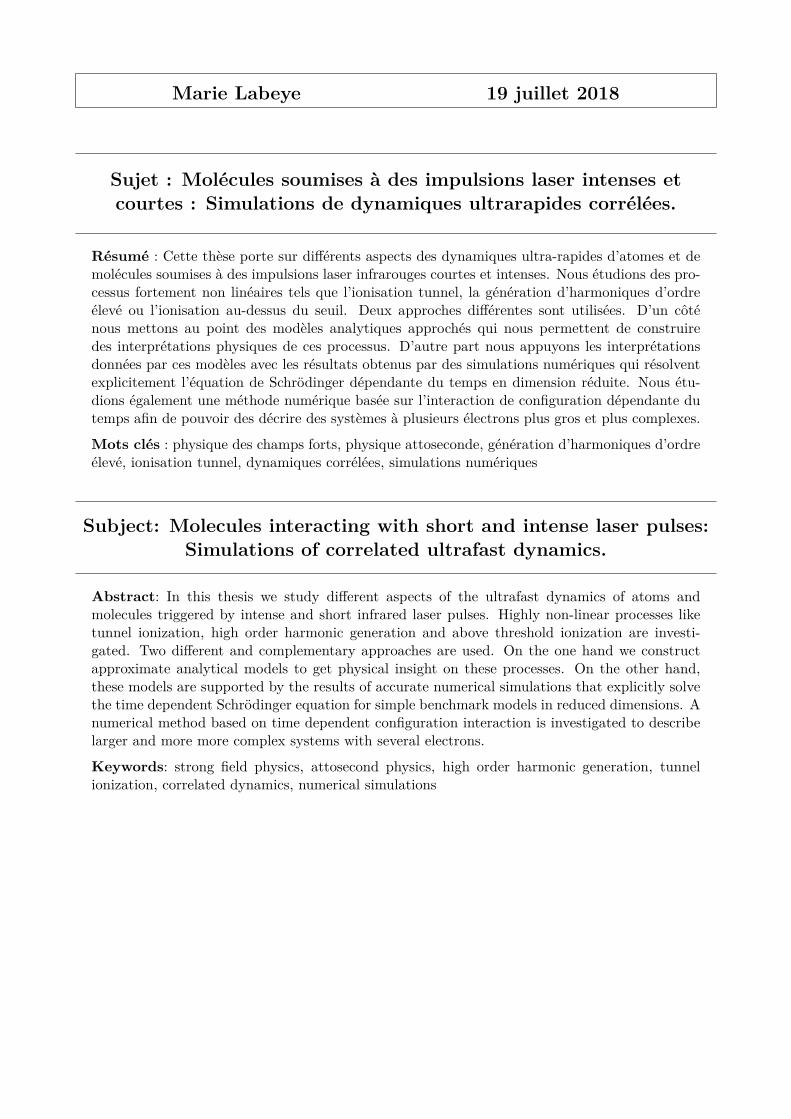
Marie Labeye 19 juillet 2018
Sujet : Molécules soumises à des impulsions laser intenses etcourtes : Simulations de dynamiques ultrarapides corrélées.
Résumé : Cette thèse porte sur différents aspects des dynamiques ultra-rapides d’atomes et demolécules soumises à des impulsions laser infrarouges courtes et intenses. Nous étudions des pro-cessus fortement non linéaires tels que l’ionisation tunnel, la génération d’harmoniques d’ordreélevé ou l’ionisation au-dessus du seuil. Deux approches différentes sont utilisées. D’un côténous mettons au point des modèles analytiques approchés qui nous permettent de construiredes interprétations physiques de ces processus. D’autre part nous appuyons les interprétationsdonnées par ces modèles avec les résultats obtenus par des simulations numériques qui résolventexplicitement l’équation de Schrödinger dépendante du temps en dimension réduite. Nous étu-dions également une méthode numérique basée sur l’interaction de configuration dépendante dutemps afin de pouvoir des décrire des systèmes à plusieurs électrons plus gros et plus complexes.
Mots clés : physique des champs forts, physique attoseconde, génération d’harmoniques d’ordreélevé, ionisation tunnel, dynamiques corrélées, simulations numériques
Subject: Molecules interacting with short and intense laser pulses:Simulations of correlated ultrafast dynamics.
Abstract: In this thesis we study different aspects of the ultrafast dynamics of atoms andmolecules triggered by intense and short infrared laser pulses. Highly non-linear processes liketunnel ionization, high order harmonic generation and above threshold ionization are investi-gated. Two different and complementary approaches are used. On the one hand we constructapproximate analytical models to get physical insight on these processes. On the other hand,these models are supported by the results of accurate numerical simulations that explicitly solvethe time dependent Schrödinger equation for simple benchmark models in reduced dimensions. Anumerical method based on time dependent configuration interaction is investigated to describelarger and more more complex systems with several electrons.
Keywords: strong field physics, attosecond physics, high order harmonic generation, tunnelionization, correlated dynamics, numerical simulations
Related Documents


![Fragmentation of CD induced by intense ultrashort …intensity, as determined by a frequency resolved autocorrela-tion (FRAC) measurement [45,46]] Fourier transform limited (FTL) pulses](https://static.cupdf.com/doc/110x72/5fea9ead36d7801864349bb3/fragmentation-of-cd-induced-by-intense-ultrashort-intensity-as-determined-by-a.jpg)


