Molecular simulation course: exercises

Molecular Simulation Course:Exercises

Thijs J.H. Vlugt, Maddalena Venturoli, Daan Frenkel and Berend Smit

Department of Chemical Engineering, University of AmsterdamNieuwe Achtergracht 166, 1018 WV Amsterdam, The Netherlands

This document describes the exercises for the Molecular Simulation Course by Berend Smit andDaan Frenkel. This document and the accompanying programs are available on the web [1].

Version 4.0, July 27, 2000.

Contents

1 Introduction 1

2 Statistical Mechanics 32.1 Distribution of particles . . . . . . . . . . . . . . . . . . . . . . . . . . . . . . . . . 32.2 Boltzmann distribution . . . . . . . . . . . . . . . . . . . . . . . . . . . . . . . . . . 32.3 Coupled harmonic oscillators . . . . . . . . . . . . . . . . . . . . . . . . . . . . . . 42.4 Random Walk on a 1D lattice . . . . . . . . . . . . . . . . . . . . . . . . . . . . . . 42.5 Random Walk on a 2D lattice . . . . . . . . . . . . . . . . . . . . . . . . . . . . . . 5

3 Basic Monte Carlo techniques 73.1 Calculation of � . . . . . . . . . . . . . . . . . . . . . . . . . . . . . . . . . . . . . . 73.2 The photon gas . . . . . . . . . . . . . . . . . . . . . . . . . . . . . . . . . . . . . . 73.3 Hard disks in a square . . . . . . . . . . . . . . . . . . . . . . . . . . . . . . . . . . 83.4 MC of a Lennard-Jones system . . . . . . . . . . . . . . . . . . . . . . . . . . . . . 93.5 Scaling . . . . . . . . . . . . . . . . . . . . . . . . . . . . . . . . . . . . . . . . . . . 93.6 Ewald summation . . . . . . . . . . . . . . . . . . . . . . . . . . . . . . . . . . . . . 103.7 Parallel tempering . . . . . . . . . . . . . . . . . . . . . . . . . . . . . . . . . . . . . 11

4 Basic Molecular Dynamics techniques 134.1 MD of a Lennard-Jones system . . . . . . . . . . . . . . . . . . . . . . . . . . . . . 134.2 Parallel MD . . . . . . . . . . . . . . . . . . . . . . . . . . . . . . . . . . . . . . . . 15

5 MD and MC in various ensembles 175.1 Barrier crossing (Part 1) . . . . . . . . . . . . . . . . . . . . . . . . . . . . . . . . . 175.2 MC in the NPT ensemble . . . . . . . . . . . . . . . . . . . . . . . . . . . . . . . . . 185.3 Ising model . . . . . . . . . . . . . . . . . . . . . . . . . . . . . . . . . . . . . . . . 19

6 Phase equilibrium and free energy calculations 216.1 Vapor-liquid equilibrium . . . . . . . . . . . . . . . . . . . . . . . . . . . . . . . . . 216.2 Umbrella sampling . . . . . . . . . . . . . . . . . . . . . . . . . . . . . . . . . . . . 22

7 Rare events 237.1 Barrier crossing (Part 2) . . . . . . . . . . . . . . . . . . . . . . . . . . . . . . . . . 237.2 Transition Path Sampling . . . . . . . . . . . . . . . . . . . . . . . . . . . . . . . . 24

7.2.1 Introduction . . . . . . . . . . . . . . . . . . . . . . . . . . . . . . . . . . . . 247.2.2 MC sampling from the distribution F (x0; T) . . . . . . . . . . . . . . . . . 267.2.3 Model system . . . . . . . . . . . . . . . . . . . . . . . . . . . . . . . . . . . 277.2.4 Questions . . . . . . . . . . . . . . . . . . . . . . . . . . . . . . . . . . . . . 27

iv Contents

8 Configurational-Bias Monte Carlo 298.1 CBMC of a single chain . . . . . . . . . . . . . . . . . . . . . . . . . . . . . . . . . . 298.2 CBMC of a simple system . . . . . . . . . . . . . . . . . . . . . . . . . . . . . . . . 318.3 Overlapping distribution for polymers . . . . . . . . . . . . . . . . . . . . . . . . . 32

9 Appendix A: Introduction to GNU/Linux 35

10 Appendix B: Introduction to FORTRAN77 39

11 Appendix C: Introduction to MOLMOL 43

12 Appendix D: Thermodynamic equations 45

13 Appendix E: Equations of motion from the Lagrangian or Hamiltonian 4713.1 Introduction . . . . . . . . . . . . . . . . . . . . . . . . . . . . . . . . . . . . . . . . 4713.2 Lagrangian . . . . . . . . . . . . . . . . . . . . . . . . . . . . . . . . . . . . . . . . . 4813.3 Example . . . . . . . . . . . . . . . . . . . . . . . . . . . . . . . . . . . . . . . . . . 5013.4 Hamiltonian . . . . . . . . . . . . . . . . . . . . . . . . . . . . . . . . . . . . . . . . 50

14 Appendix F: Questions about the book “Understanding ..” [2] 5314.1 Introduction to FORTRAN77 . . . . . . . . . . . . . . . . . . . . . . . . . . . . . . 5314.2 Chapter 2 . . . . . . . . . . . . . . . . . . . . . . . . . . . . . . . . . . . . . . . . . . 5314.3 Chapter 3 . . . . . . . . . . . . . . . . . . . . . . . . . . . . . . . . . . . . . . . . . . 5714.4 Chapter 4 . . . . . . . . . . . . . . . . . . . . . . . . . . . . . . . . . . . . . . . . . . 5714.5 Chapter 5 . . . . . . . . . . . . . . . . . . . . . . . . . . . . . . . . . . . . . . . . . . 5814.6 Chapter 6 . . . . . . . . . . . . . . . . . . . . . . . . . . . . . . . . . . . . . . . . . . 5914.7 Chapter 7 . . . . . . . . . . . . . . . . . . . . . . . . . . . . . . . . . . . . . . . . . . 5914.8 Chapter 8 . . . . . . . . . . . . . . . . . . . . . . . . . . . . . . . . . . . . . . . . . . 6014.9 Chapter 11 . . . . . . . . . . . . . . . . . . . . . . . . . . . . . . . . . . . . . . . . . 6114.10Chapter 13 . . . . . . . . . . . . . . . . . . . . . . . . . . . . . . . . . . . . . . . . . 61

15 Appendix G: Possible research projects 6315.1 Adsorption in porous media . . . . . . . . . . . . . . . . . . . . . . . . . . . . . . . 6315.2 Transport properties in liquids . . . . . . . . . . . . . . . . . . . . . . . . . . . . . 6315.3 Parallel Molecular Dynamics . . . . . . . . . . . . . . . . . . . . . . . . . . . . . . 6415.4 Phase diagram of ethane . . . . . . . . . . . . . . . . . . . . . . . . . . . . . . . . . 6515.5 Diffusion in a porous media . . . . . . . . . . . . . . . . . . . . . . . . . . . . . . . 6515.6 Multiple time step integrators . . . . . . . . . . . . . . . . . . . . . . . . . . . . . . 6615.7 Thermodynamic integration . . . . . . . . . . . . . . . . . . . . . . . . . . . . . . . 6715.8 Hints for programming . . . . . . . . . . . . . . . . . . . . . . . . . . . . . . . . . . 68

16 Appendix H: Software 71

Acknowledgements 73

Bibliography 75

Chapter 1

Introduction

This documents describes the exercises for the Molecular Simulation Course by Daan Frenkeland Berend Smit. To do the exercises, it is essential to have a copy of the book “UnderstandingMolecular Simulation” by Daan Frenkel and Berend Smit [2]. Some of the exercises in this doc-ument were taken from several standard textbooks [2–6].

In most of the exercises, some programming has to be done. One does not have to write aprogram from scratch, but rather one has to make some small modifications to an existing code�. We have programmed the code in FORTRAN77 because it is quite easy to learn. However,the random number generator that is used in some of the programs is written in C [7]. See,for example, ref. [8] for more information about random number generators. All programs areprovided with a makefile that has been prepared for GNU/Linux using the g77/gcc compil-ers [9, 10]. Compiling the programs on other Unix systems is straightforward. Solutions of theprogramming exercises as well as the LATEX source of this document are available on request.

The course and exercises are divided into several parts:

� Introduction to Unix and FORTRAN77 (0.5 day)

� Basic Statistical Mechanics (1.5 day)

� Basic Monte Carlo (MC) techniques (2 days)

� Basic Molecular Dynamics (MD) techniques (2 days)

� MD and MC in various ensembles (1 day)

� Phase equilibrium and free energy calculations (1 day)

� Rare events (1 day)

� Configurational-Bias Monte Carlo (1 day)

We have setup the course in such a way that lectures are given every morning (3 hours),while the exercises have to be done in the afternoon (5 hours); we do not expect that all studentshave enough time to complete all exercises. After all exercises have been completed, a specialresearch project has to be done (duration: 2 weeks) to pass the exam. In Appendix G, we havegiven some suggestions for research projects. We have also included a list of questions about

�Although the text may suggest otherwise, all programs do not have to be written from scratch. For more infor-mation, see the README file from the distribution.

2 Introduction

the book of Daan Frenkel and Berend Smit [2] (Appendix F).

We have done our best to remove all errors from this document and the programs. However,we have to make the following statement:

“We make no warranties that this document or the programs accompanied by this documentare free of error, or that they will meet your requirements for any particular application. Theauthors disclaim all liability for direct and consequential damages resulting from the use of thisdocument or the programs accompanied by this document. It is not allowed to distribute thisdocument and the accompanying programs.”

We are interested in what you think about this course. Any comment would be appreciated,even severe criticism. Comment can be send to Berend Smit.

Contact address:

Berend SmitDepartment of Chemical EngineeringUniversity of AmsterdamNieuwe Achtergracht 1661018 WV Amsterdam, The Netherlandsemail: [email protected]: http://molsim.chem.uva.nl

Chapter 2

Statistical Mechanics

2.1 Distribution of particles

Consider an ideal gas of N particles in a constant volume at constant energy. Let us divide thevolume in p identical compartments. Every compartment contains ni molecules such that

N =

i=pXi=1

ni (2.1)

An interesting quantity is the distribution of molecules over the p compartments. Because theenergy is constant, every possible eigenstate of the system will be equally likely. This meansthat in principle it is possible that one of the compartments is empty.

1. Enclosed is a program that calculates the distributions of molecules along the p compart-ments. Run the program for different numbers of compartments (p) and total number ofgas molecules (N). Note that the code has to be completed first (see the file distribution.f).The output of the program is the probability to find x particles in a particular compartmentas a function of x. This is printed in the file output.dat, which can be plotted using xmgr-nxy output.dat (the option -nxy means that more than one column is plotted).

2. Why does it (almost) never happen that one of the compartments is empty ?

3. Consider the case of p = 2. The probability of finding n1 molecules in compartment 1 andn2 = N - n1 molecules in compartment 2 is given by

P (n1) =N!

n1!� (N - n1) !� 2N(2.2)

Compare your numerical results results with the analytical solution for different values ofN. Show that this distribution is a Gaussian for small n1. Hint: For x > 10, it might beuseful to use Stirling’s approximation:

x! � (2�)12 xx+

12 exp [-x] (2.3)

2.2 Boltzmann distribution

Consider a system of N energy levels with energies 0; �; 2�; � � � ; (N - 1)� � and � > 0.

4 Statistical Mechanics

Questions:

1. Calculate, using the given program, the occupancy of each level for different values of thetemperature. What happens at high temperatures ?

2. Change the program in such a way that the degeneracy of energy level i equals i+1. Whatdo you see ?

3. Modify the program in such a way that the occupation of the energy levels as well as thepartition function (q) is calculated for a linear rotor with moment of inertia I. Compareyour result with the approximate result

q =2I

�h2(2.4)

for different temperatures. Note that the energy levels of a linear rotor are

U = J (J+ 1)h2

2I(2.5)

with J = 0; 1; 2; � � � ;1. The degeneracy of level J equals 2J+ 1.

2.3 Coupled harmonic oscillators

Consider a system of N harmonic oscillators with a total energy U. A single harmonic oscillatorhas energy levels 0; �; 2�; � � � ;1 (� > 0). All harmonic oscillators in the system can exchangeenergy.

Questions:

1. Invent a computational scheme for the update of the system at constant total energy (U).Compare your scheme with the scheme that is incorporated into the given computer code(see the file harmonic.f).

2. Make a plot of the energy distribution (output.dat) of the first oscillator as a function of thenumber of oscillators for a constant value of U=N. Which distribution is recovered whenN becomes large ? What is the function of the other N- 1 harmonic oscillators ? Explain.

3. Compare this distribution which the canonical distribution of a single oscillator at thesame average energy.

4. How does this exercise relate to the derivation of the Boltzmann distribution for a systemat temperature T on page 12 of ref. [2] ?

2.4 Random Walk on a 1D lattice

Consider the random walk of a single particle on a line. The probability that after N jumps thenet distance of the particle equals n, is:

ln (P (n;N)) � 1

2ln�

2

�N

�-

n2

2N(2.6)

2.5 Random Walk on a 2D lattice 5

Questions:

1. Derive this equation. The probability to jump to one direction equals the probability tojump to the other direction. For large x, x! can be approximated by:

x! � (2�)12 xx+

12 exp [-x] (2.7)

2. Compare this theoretical result with the computed root mean square displacement and thecomputed function P (n;N) (see the file output.dat). What is the diffusivity of this system ?

3. Modify the program in such a way that the probability to jump in one direction equals 0:8.What happens ?

2.5 Random Walk on a 2D lattice

Consider the random walk of N particles on a M �M lattice. Two particles cannot occupy thesame lattice site. On this lattice, periodic boundaries are used. This means that when a particleleaves the lattices it returns on the opposite side of the lattice.

Questions:

1. What is the fraction occupied sites (�) of the lattice as a function of M and N ?

2. Make a plot of the diffusivity D as a function of � for M = 32. For low values of �, thediffusivity can be approximated by

D � D0 (1- �) (2.8)

Derive this equation. Why is this equation not exact ?

3. Modify the program in such a way that the probability to jump in one direction is largerthan the probability to jump in the other direction. Explain the results.

4. Modify the program in such a way that periodic boundary conditions are used in onedirection only. What happens ?

5. Modify the program in such a way that a certain fraction of the particles are “frozen”.Investigate the influence of the fraction of frozen particles on the diffusivity.

Chapter 3

Basic Monte Carlo techniques

3.1 Calculation of �

Consider a circle of diameter d surrounded by a square of length l (l � d). Random coordinateswithin the square are generated. The value of � can be calculated from the fraction of pointsthat fall within the circle.

Questions:

1. How can � be calculated from the fraction of points that fall in the circle ? Remark: the“exact” value of � can be computed numerically using � = 4� arctan (1).

2. Complete the small Monte Carlo program to calculate � using this method.

3. How does the accuracy of the result depend on the ratio l=d and the number of generatedcoordinates ? Derive a formula to calculate the relative standard deviation of the estimateof �.

4. Is it a good idea to calculate many decimals of � using this method ?

3.2 The photon gas

The average occupancy number of state j of the photon gas (hnji) can be calculated analytically;see equation 14.13. However, it is also possible to compute this quantity using a Monte Carloscheme. In this exercise, we will use the following procedure to calculate hnji:

1. Start with an arbitrary nj

2. Decide at random to perform a trial move to increase or decrease nj by 1.

3. Accept the trial move with probability

acc (o! n) = min (1; exp [-� (U (n) -U (o))]) (3.1)

Of course, nj cannot become negative !

8 Basic Monte Carlo techniques

Questions:

1. How can this scheme obey detailed balance when nj = 0 ? After all, nj can not becomenegative !

2. Is the algorithm still correct when trial moves are performed that change nj with a randominteger from the interval [-5; 5] ? What happens when only trial moves are performed thatchange nj with either -3 or +3 ?

3. Assume that N = 1 and �j = �. Write a small Monte Carlo program to calculate hnji as afunction of ��. Compare your result with the analytical solution.

4. Modify the program in such a way that the averages are updated only after an acceptedtrial move. Why does this lead to erroneous results ? At which values of � does this errorbecome more pronounced ?

5. Modify the program in such a way that the distribution of nj is calculated as well. Com-pare this distribution with the analytical distribution.

3.3 Hard disks in a square

Consider a system of N identical hard disks with diameter 1 in a square of size 10. No periodicboundary conditions are applied. The energy of this system (U) is either U = 0 (no overlaps) orU = 1 (at least one overlap). We would like to calculate the radial distribution function of thedisks (g (r) ; r < 5) in the canonical ensemble. There are 2 methods of calculating this:

1. Dynamic scheme.The disks are initially placed on a lattice and trial moves are performed to translate thedisks. A trial move is accepted when there are no overlaps and rejected when there areone or more overlaps.

2. Static Scheme.In every cycle, all disks are put at a completely random position in the system. The radialdistribution function of this configuration is calculated and multiplied by the Boltzmannfactor of the system (0 when there is at least one overlap and 1 when there are no overlaps).

Questions:

1. Write a program to calculate g (r) using both methods (see sample.f). Make sure that bothmethods give the same result when N is small. Use the MOLMOL program to visualizethe Monte Carlo simulation.

2. At which N does the second method starts to fail ? Why ?

3. For which method will there be a larger correlation between successive elements of theMarkov chain ? Explain.

3.4 MC of a Lennard-Jones system 9

3.4 MC of a Lennard-Jones system

In this exercise, we will study a 3D Lennard-Jones system. See also Case Study 1 from ref. [2].

Questions:

1. In the present code, the pressure of the system is not calculated. Modify the code in sucha way that the average pressure can be calculated. You will only have to make somemodifications in the subroutine ener.f.

2. Perform a simulation at T = 2:0 and various densities. Up to which density does the idealgas law

�p = � (3.2)

hold ?

3. The program produces a sequence of snapshots of the state of the system. Try to visualizethese snapshots using the program MOLMOL.

4. For the heat capacity at constant volume one can derive

Cv =

U2�- hUi2

kBT2(3.3)

in which U is the total energy of the system. Derive a formula for the dimensionless heatcapacity. Modify the program (only in mc nvt.f) in such a way that Cv is calculated.

5. Instead of performing a trial move in which only one particle is displaced, one can do atrial move in which all particles are displaced. Compare the maximum displacements ofthese moves when 50% of all displacements are accepted.

6. Instead of using a uniformly distributed displacement, one can also use a Gaussian dis-placement. Does this increase the efficiency of the simulation ?

3.5 Scaling

Consider a system in which the energy is a function of one variable (x) only:

exp [-�U (x)] = � (x)� (1- x) (3.4)

in which � (x) is the Heaviside step function: � (x < 0) = 0 and � (x > 0) = 1. We wouldlike to calculate the distribution of x in the canonical ensemble. We will consider two possiblealgorithms (we will use Æ > 0):

1. Generate a random change in x between [-Æ; Æ]. Accept or reject the new x according to itsenergy.

2. Generate a random number � between [1; 1 + Æ]. With a probability of 0:5, decide to invert� or not. The new value of x is obtained by multiplying x with �.

10 Basic Monte Carlo techniques

Questions:

1. Derive the correct acceptance/rejection rules for both schemes.

2. Complete the computer code to calculate the probability density of x. The program writesthis distribution to distri.dat.

3. What happens when the acceptance rule of method 1 is used in the algorithm of method 2? Why ?

3.6 Ewald summation

An example of long-range interactions is the coulombic potential between point charges:

U (rij) =qiqj

4��0rij(3.5)

Special techniques like the Ewald summation are required to compute the total potential energycorrectly. When the Ewald summation is used, the total potential energy (Ut) consists of threecontributions: the fourier space part (Uf), the real space part (Ur), and the self energy (Us):

Ut = Uf +Ur +Us

Uf =1

2V�0

1Xk 6=0

exp�-k2=4�2

�k2

�����i=NXi=1

exp [-ik � ri]

�����2

Ur =1

4��0

Xi<j

qiqjerfc (�rij)

rij

Us = -1

4��0

i=NXi=1

q2i�p�

(3.6)

in whichN is the number of ions andV is the volume of the (rectangular) unit-cell. The positionsof the ions in the unit-cell are indicated by ri. The complementary error function (erfc (x) =2p�� R1

xdt exp

�-t2

�) falls to zero with increasing x. Details of the Ewald summation can be

found in ref. [2].Consider a simple cubic lattice (for example, NaCl) in which the kations are located at

[0; 0; 0], [1; 1; 0], [1; 0; 1], and [0; 1; 1] and the anions are located at [0; 0; 1], [1; 1; 1], [1; 0; 0], and[0; 1; 0]. The total energy of an infinitely large NaCl crystal equals:

U = -nq2M

4��0r0(3.7)

in which r0 is the closest distance between ion pairs, n is the number of ion pairs and M is theMadelung constant.

Questions:

1. What is the relation between Ut and the coulombic virial ?

2. How many ion pairs are present in a unit-cell of NaCl ?

3.7 Parallel tempering 11

3. Compute the Madelung constant of NaCl using the given program. Make a plot of thetotal energy as a function of k for different values of �. What is a good choice for � andk ? You will have to program the real space part of the Ewald summation yourself (inrealspace.f). Note: We will use r0 = 1, 4��0 = 1 and qNa+ = -qCl- = 1.

4. Rewrite the program in such a way that each ion is given a random displacement fromthe interval [-0:3; 0:3] (this may correspond to a liquid structure). Make a plot of the totalenergy as a function of k for different values of �.

5. Consider a system of dipolar molecules AB (qA = -qB 6= 0). What will happen withthe radial distribution function when a truncated and shifted coulombic potential is usedinstead of the Ewald summation ?

3.7 Parallel tempering

The method of parallel tempering [11–14] is a Monte Carlo scheme that has been derived toachieve good sampling of systems that have a free energy landscape with many local minima.

In parallel tempering we consider N systems. In each of these systems we perform a simula-tion in the canonical ensemble, but each system is in a different thermodynamic state. Usually,but not necessarily, these states differ in temperature. In what follows we assume that this is thecase. Systems with a sufficiently high temperature pass all barriers in the system. The low tem-perature systems, on the other hand, mainly probe the local energy minima. The idea of paralleltempering is to include MC trial moves that attempt to “swap” systems that belong to differentthermodynamic states, e.g., to swap a high temperature system with a low temperature system.If the temperature difference between the two systems is very large, such a swap has a very lowprobability of being accepted. This is very similar to particle displacement in ordinary MonteCarlo. If one uses a very large maximum displacement a move has a very low probability of be-ing accepted. The solution to this problem is to use many small steps. In parallel tempering weuse intermediate temperatures in a similar way. Instead of making attempts to swap betweena low and a high temperature, we swap between ensembles with a small temperature difference.

The total partition function of a system with N canonical subsystems (Q) equals

Q =

i=NYi=1

Qi (3.8)

in which Qi is the canonical partition function of the individual system i

Qi =Xxi

exp [-�iU (xi)] (3.9)

in which �i = 1= (kBTi). For each of these systems, individual trial moves are performed. Aftera randomly selected number of trial moves, an attempt is made to exchange configurations.Two systems (i and j, ji- jj = 1) are selected at random, the systems are exchanged by choosingxi (n) = xj (o) and xj (n) = xi (o). The ratio of acceptance probabilities equals

acc (o! n)

acc (n! o)= exp [(�i - �j)� (U (xi (o)) -U (xj (o)))] (3.10)

Such trial moves will be accepted when there is enough overlap between the energies of systemsi and j. To demonstrate this technique, consider a two dimensional system of 9 particles that are

12 Basic Monte Carlo techniques

confined in a square (� = 2:5). Each particle pair interact with a soft repulsive potential:

U (r) =

�� (r- 1)2 r � 1

0 r > 1(3.11)

We will use � = 1. At low temperatures, the particles are not able to pass each other and there-fore a particle is confined at its original position. However, in principle the distribution of theposition of a particle should be symmetrical.

Questions:

1. Derive equation 3.10.

2. Compute the distribution of the position of the first particle as well as the distribution ofthe total energy for T = 0:001 when no exchange moves are allowed (N = 1). At whichtemperature are the particles allowed to diffuse ?

3. Complete the code for the exchange moves and find out how many systems are neededto ensure that for T = 0:001 the particle is allowed to diffuse. You will have to check thedistribution of the total energy to ensure that there is enough overlap between the systems.

4. At high temperature, confirm that the equilibrium distributions with and without ex-change moves are identical.

Chapter 4

Basic Molecular Dynamics techniques

4.1 MD of a Lennard-Jones system

Enclosed is a Molecular Dynamics (MD) program for a Lennard-Jones fluid in the NVE ensem-ble. Unfortunately, the program does not conserve the total energy because it contains threeerrors.

Questions:

1. Find the three errors in the code. The person that spots the errors first will receive a bottleof French wine from Berend Smit (people from Berend’s group are excluded from thiscontest). Hint: there are two errors in integrate.f and one in force.f. See the file system.inc fordocumentation about some of the variables used in this code.

2. How is one able to control the temperature in this program ? After all, the total energy ofthe system should be constant (not the temperature).

3. To test the energy drift �U of the numerical integration algorithm for a given time step �t

after N integration steps, one usually computes [15]

�U (�t) =1

N

i=NXi=1

����U (0) -U (i�t)

U (0)

���� (4.1)

In this equation,U (x) is the total energy (kinetic+potential) of the system at time x. Changethe program (only in mdloop.f) in such a way that �U is computed and make a plot of �Uas a function of the time step. How does the time step for a given energy drift change withthe temperature and density ?

4. One of the most time consuming parts of the program is the calculation of the nearestimage of two particles. In the present program, this calculation is performed using an if-then-else-endif construction. This works only when the distance between two particles issmaller than 1:5 and larger than -1:5 times the size of the periodic box. A way to overcomethis problem is to use a function that calculates the nearest integer nint

x = x- box � nint (x � ibox) (4.2)

in which ibox = 1:0=box. Which expression is faster ? (Hint: You only have to make somemodifications in force.f) Which expression will be faster on a vector computer like a Cray

14 Basic Molecular Dynamics techniques

C90 ? Because the nint function is usually slow, you can write your own nint function.For example, when x < -998, we can use

nint (x) = int (x+ 999:5) - 999 (4.3)

What happens with the speed of the program when you replace the standardnint function? Do you have an explanation for this � ?

5. In equation 4.2, ibox is used instead of 1=box. Why ?

6. An important quantity of a liquid or gas is the so called self diffusivity D. There are twomethods to calculate D:

(a) by integrating the velocity autocorrelation function:

D =1

3

Z1

0

Dv (t) � v

�t + t

0�E

dt0

=

R1

0

Pi=Ni=1

Dv (i; t) � v

�i; t+ t

0�E

dt0

3N(4.4)

in which N is the number of particles and v (i; t) is the velocity of particle i at timet. One should choose t in such a way that independent time origins are taken, i.e.t = ia�t, i = 1; 2; � � � ;1 and hv (t) � v (t+ a�t)i � 0 (why ?).

(b) by calculating the mean square displacement:

D = limt0!1

����x�t + t0�- x (t)

���2�6t

0 (4.5)

One should be very careful with calculation of the mean square displacement whenparticles are always transformed to the central box (why ?).

Modify the program in such a way that the self diffusivity can be calculated using bothmethods. Only modifications in subroutine sample diff.f are needed. Why is it importantto use only independent time origins for the calculation of the means square displacementand the velocity autocorrelation function ? What is the unit of D in SI units ? How can onetransform D into dimensionless units ?

7. For Lennard-Jones liquids, Naghizadeh and Rice report the following equation for the selfdiffusivity (dimensionless units, T� < 1:0 and p� < 3:0) [16]

10log (D�) = 0:05 + 0:07p� -1:04 + 0:1p�

T�(4.6)

Try to confirm this equation with simulations. How can one translate D� to a diffusivityin SI units ?

8. Instead of calculating the average energy hUi directly, one can use the radial distributionfunction g (r). Derive an expression for hUi using g (r). Compare this calculation with adirect calculation of the average energy. A similar method can be used to compute theaverage pressure.

�The result will strongly depend on the computer/compiler that is used.

4.2 Parallel MD 15

9. In the current version of the code, the equation of motion are integrated by the Verletalgorithm. Make a plot of the energy drift �U for the following integration algorithms [2]:

� Verlet

� Velocity Verlet [17]

� Euler (never use this one except here !!!)

4.2 Parallel MD

Please find enclosed a parallel version of the code of the previous exercise. This code is writtenin FORTRAN77 using an MPI library. We will use LAM [18] for this. To run the program inparallel, several things have to be done:

1. Copy the file mpif.h from $fLAMHOMEg/h. This file is strongly dependent on the versionof MPI.

2. Compile the code using LAM. The commands hf77 and hcc will use the GNU compilersg77 and gcc to compile the source.

3. Find out on how many computers you would like to run the code. The user must be ableto remotely execute on the machine with rsh. Remote host permission must be provided ineither /etc/hosts.equiv or the remote user’s �/.rhosts file. The remote user’s shell must havea search path that will locate LAM executables and the remote shell’s startup file must notprint anything to standard error when invoked non-interactively.

4. Type recon -v hostnames in which the file hostnames should contain the hostnames of allmachines that will be used.

5. When no errors occur, you can start the LAM daemon by typing lamboot -v hostnames.When this is successful too, you can start the run-script. Beware that the command mpirunuses an absolute path !

6. After the execution is completed, the LAM daemon can be killed by typing wipe -v host-names.

Questions:

1. Try to find out which part of the calculation is performed in parallel.

2. In the file force.f, there is a line:

do I=(Iirank+1),(Npart-1),Iisize

In principle, the program also works correct when this line is replaced by:

do I=((Iirank*(Npart-1)/Iisize) + 1),((Iirank+1)*(Npart-1)/Iisize)

What is the difference between these two methods and how is this reflected in the scalingof the code ? Hint: Npart is the number of particles, Iisize is the number of processors andIirank is the index of a particular processor (Iirank = 0; 1; 2; � � � ; Iisize - 1).

3. Run the code on different numbers of nodes and record the execution time as a functionof the number of nodes. What happens when using a large number of nodes ?

16 Basic Molecular Dynamics techniques

4. Perform this calculation again for a much larger system at the same density. What do yousee ?

5. Can you come up with a better strategy to parallelize this code ?

6. Can the same strategy be used for a MC simulation of the same system in the canonicalensemble ?

Chapter 5

MD and MC in various ensembles

5.1 Barrier crossing (Part 1)

Consider the movement of a single particle that moves on a 1D potential energy surface withthe following functional form:

U (x) =

8<:

�Bx2 x < 0

� (1 - cos (2�x)) 0 � x � 1

�B (x- 1)2 x > 1

(5.1)

The energy, force and the derivative of the force are continuous functions of the position x and� > 0.

Questions:

1. Derive an expression for B. Make a sketch of the energy landscape.

2. A program is provided that integrates the equation of motion of the particle starting atx (t = 0) = 0 using several methods:

(a) No thermostat (NVE ensemble). What do you expect the phase space trajectories tolook like ?

(b) Andersen thermostat. In this method, the velocity of the particle is coupled to astochastic heat bath which leads to a canonical distribution.

(c) A Nose-Hoover chain [15, 19]. In this method, the motion of the particle is coupledto a chain of thermostats. The equations of motion are integrated using an explicittime-reversible algorithm that might look a little-bit complicated at first sight [15],see integrate res.f. One can prove that this method yields a canonical distributionprovided that the system is ergodic.

(d) No molecular dynamics, but a simple Monte Carlo scheme.

The Andersen thermostat and the NVE integration algorithm are not implemented yet, soyou will have to do this yourself (see integrate nve.f and integrate and.f). Try to use allmethods for a low temperature, T = 0:05, for which the system behaves like a harmonicoscillator. Pay special attention to the following:

(a) Why does the phase space distribution of the MC scheme look so much different atlow temperatures ?

18 MD and MC in various ensembles

(b) Why does the phase space distribution of the NVE scheme look like a circle ?

(c) Compare the phase space distributions of the Nose-Hoover chain method with distri-bution generated by the Andersen thermostat. How long has the Nose-Hoover chainto be to obtain a canonical distribution ?

3. Investigate at which temperature the particle is able to cross the energy barrier.

4. Another widely used algorithm is the “temperature coupling” of Berendsen [20]. It isimportant to note that this method does not produce a canonical ensemble and thereforewe should never use it. In this algorithm, the temperature of the system is controlled byscaling the velocities every time step with a factor �

� =

�1+

�t

�T

�T0

T- 1

��12

(5.2)

in which T0 is the desired temperature, T is the actual temperature, �t is the time step ofthe integration algorithm and �T is a constant. The temperature coupling algorithm canbe used in combination with a Leap-Frog algorithm

v

�t+

�t

2

�= �

�t-

�t

2

���v

�t -

�t

2

�+F (t)

m�t

�

x (t +�t) = x (t) + v

�t+

�t

2

��t (5.3)

Compare the distributions of the Berendsen temperature bath with the canonical distribu-tions.

5. Modify the program in such a way that the potential energy function

U = � (1 - cos (2�x)) (5.4)

is used. Calculate the diffusion coefficient as a function of the temperature. Why is itimpossible to calculate the diffusivity at low temperatures using ordinary molecular dy-namics ? Why is the diffusion coefficient obtained by using the Andersen thermostat afunction of the collision frequency ?

5.2 MC in the NPT ensemble

Enclosed is a program to simulate hard spheres (diameter 1) in the NPT ensemble using MC.

Questions:

1. Why is it impossible to calculate the virial for this system directly ?

2. In the current code, a random walk is performed in ln (V) instead of V. Change the codein such a way that a random walk in V is performed. Check that the average densitiescalculated by both algorithms are equal.

3. Make a plot of the acceptance ratio for volume displacements as a function of the maxi-mum volume displacement for both algorithms.

5.3 Ising model 19

5.3 Ising model

In this exercise we consider a 2D Ising model. In this model, N spins s (�1) are arranged on alattice. Every spin (i) has 4 neighbors (j = 1; 2; 3; 4). The total energy of the system equals

U = -�

2

i=NXi=1

j=4Xj=1

sisj (5.5)

in which si = �1 and � > 0. The second summation is a summation over all spin pairs of spini. The total magnetization M equals the sum over all spins:

M =

i=NXi=1

si (5.6)

The 2D Ising model has a critical point close to �c � 0:44.

Questions:

1. Complete the given simulation code for this system (see ising.f).

2. Calculate the distribution of M for N = 32� 32 and � = 0:5 in the canonical ensemble. Inprinciple, this distribution should be symmetrical:

p (M) = p (-M) (5.7)

Why does this not seem to be the case ?

3. Instead of a simulation in the canonical ensemble, one can perform the simulation in theensemble �:

� / exp [-�U +W (M)] (5.8)

The average value of an observable O in the canonical ensemble equals:

hOi = hO exp [-W (M)]i�hexp [-W (M)]i�

(5.9)

in which h� � � i� is an ensemble average in the ensemble �. Derive this equation.

4. Perform simulations with some given distributions W (M) (w.type1.dat and w.type2.dat).Explain your results. How should one choose the function W (M) to obtain the optimalefficiency ?

5. What happens when W (M) is a Gaussian,

W (M) = A exp

"-

�M

�

�2#(5.10)

with A > 0 ?

6. What happens when W (M) = W (U) = -�U ?

Chapter 6

Phase equilibrium and free energycalculations

6.1 Vapor-liquid equilibrium

In this exercise, we will use Widom’s test particle method to locate a vapor-liquid equilibrium.This is compared with a Gibbs-ensemble simulation.

Questions:

1. Modify the Monte Carlo program of Lennard-Jones particles in theNVT ensemble (only inthe file mc nvt.f) in such a way that the chemical potential can be calculated using Widom’stest particle method:

� = �0 -ln��-1 hexp [-��U+]i�

�(6.1)

in which � is the number of particles per volume, U+ is the energy of a test particle and

�0 =- ln

��3�

�(6.2)

� Make a plot of the chemical potential and pressure as a function of the density forT = 0:8.

� Why is it more difficult to calculate the chemical potential at high densities than atlow densities ?

� How can you locate the vapor-liquid coexistence densities ?

2. Perform a Gibbs-ensemble simulation of the system at T = 0:8. In the Gibbs ensemble, thechemical potential of box i is equal to [2, 21]

�i = �0 -lnD

Vi

ni+1exp

�-��U+

i

�E�

(6.3)

in which ni is the number of particles in box i and Vi is the volume of box i. Do thevapor/liquid density and chemical potential agree with your previous results ?

22 Phase equilibrium and free energy calculations

6.2 Umbrella sampling

Consider a single particle on a one dimensional energy landscape. The energy as a function ofthe position is given by

U (x) = �x2 (6.4)

One would like to calculate the probability distribution of finding the particle at a position x

(p (x)) by using a Monte-Carlo scheme (we will use � = � = 1).

Questions:

1. Why is this distribution difficult to calculate for large values of x when a conventional MCscheme is used ?

2. Alternatively, one can divide the x axis in overlapping slices and calculate the distributionp (x; i) in all slices i. This scheme is often referred to as umbrella sampling. Show thatp (x; i) / p (x; j) when i 6= j (This also means that ln (P (x; i)) = ln (P (x; j)) +C in which C

is a constant).

3. Compare the results from the conventional MC algorithm with the results from the um-brella sampling simulations, especially at large values of x. Different slices can be com-bined by using xmgr.

Chapter 7

Rare events

7.1 Barrier crossing (Part 2)

In one of the previous exercises, we have seen that sometimes there may be energy barriers is asystem that are so high, that the crossing rate can not be calculated using conventional moleculardynamics techniques. A method that can be used to calculate the transition rate is the Chandler-Bennett approach [2,4,22,23]. We will use this approach to calculate the crossing rate of a singleparticle over an energy barrier

U (x) =

8>>>><>>>>:

1 x < -5

0 -5 � x < 0

� (1- cos (2�x)) 0 � x � 1

0 1 < x � 51 x > 5

(7.1)

We will call the region left from the barrier the reactant side A and the region right from theenergy barrier the product side B. The time dependent rate constant kA!B (t) can be writtenas [2]

kA!B (t) =hq (0) Æ (q? - q (0))� (q (t) - q?)i

hÆ (q? - q (0))i � hÆ (q? - q)ih� (q? - q)i (7.2)

We are mainly interested at the plateau value of kA!B (t), which is the hopping rate. At firstsight, this equation might look pretty horrible. First of all, we need to define our symbols:

� q is the reaction coordinate. In this case, q = x is a sensible choice. q (0) is the reactioncoordinate at t = 0.

� q? is the position of the dividing surface. We will choose 0 < q? < 1. Note that thedividing surface does not always have to be on top of the energy barrier !

� h� � � i denotes an ensemble average

� Æ (x) is Dirac’s delta function: Æ (x = 0) =1, Æ (x 6= 0) = 0,R1

-1Æ (x)dx = 1 and

Æ (h (s)) =Æ (s - s0)

jh0(s)j

(7.3)

when h (s0) = 0.

24 Rare events

� � (x) is the Heaviside step function: � (x < 0) = 0 and � (x > 0) = 1. Note that the defini-tion of � in ref. [2] on page 251 is incorrect.

Now it is a lot easier to understand what the terms in equation 7.2 mean:

� The first term on the r.h.s. is the conditional average of the product [q (0) � (q (t) - q?)]

given that the initial position is at the top of the barrier (q (0) = q?). The term � (q (t) - q?)

is equal to 1 when the particle is in state B at time t and equal to 0 otherwise. q (0) is theinitial velocity of the particle at the top of the barrier.

� The second term on the r.h.s is the probability of finding the system on top of the barrierdivided by the probability that the system is on the reactant side of the barrier.

Questions:

1. What is the unit of kA!B (t) in SI units and in dimensionless units ?

2. Is the force on a particle a continuous function of x ?

3. A program is provided to perform a Molecular Dynamics simulation for a single particleprovided that q (0) = q?. The sampling of the crossing rate has still to be programmed(see mdloop.f and sample.f).

4. Calculate the crossing rate for different temperatures and positions of q?. Make a plot ofln (kA!B) versus T-1.

5. Check that the crossing rate is independent of the location of the dividing surface.

7.2 Transition Path Sampling

In this section, we will study the Transition Path Sampling method for the calculation of rateconstants of rare events. This method is able to compute rate constants without having to as-sume a transition state. For more details about this method, the reader is referred to ref. [24,25],on which this exercise is based.

7.2.1 Introduction

Consider a dynamical system with two stable states, A and B, in which transitions from A toB are rare. The transition rate, k, from A to B can be calculated from the time derivative of anautocorrelation function C (t),

k =dC (t)

dttmol < t� trxn (7.4)

C (t) =hhA (x0)hB (xt)i

hhA (x0)i ; (7.5)

provided that the reaction time trxn of the system [A;B] is much larger than the molecular relax-ation time tmol of the system in region A or B. In equation 7.5, xt represents the momenta p andpositions q of the system at time t. We will only consider deterministic trajectories for whichxt is completely determined by the initial conditions x0, i.e. xt = xt (x0). The functions hA and

7.2 Transition Path Sampling 25

hB characterize the regions A and B; hA;B (x) = 1 when x 2 A;B, respectively, and hA;B (x) = 0

otherwise. Note that A and B must be chosen in such a way that A \ B = ?.Since the function xt is fully determined by the initial condition x0, the ensemble averages

in equation 7.5 can be written as an integration over the initial conditions weighted with theequilibrium distribution N (x0),

C (t) =

Rdx0N (x0)hA (x0)hB (xt (x0))R

dx0N (x0)hA (x0): (7.6)

We can also look at this equation as the ensemble average of hB (xt) weighted with the equi-librium distribution N (x0) � hA (x0). In other words, C (t) is the fraction of trajectories thatstart in A with distribution N (x0) and reach B after time t. Since we are sampling over pathsthis ensemble is called the path ensemble. A procedure to sample this ensemble would be toperform a MD simulation to generate a new path of length t and subsequently use a MC proce-dure to decide whether to accept or reject this new path. In this way, we generate an ensemble ofpaths which we can use to compute ensemble averages. We will only consider a micro-canonicalensemble of initial conditions x0, i.e.

N (x0) = Æ (N (x0) - E) (7.7)

in which E is the total energy. In principle we could compute C (t) from an “ordinary” pathensemble simulation. This would imply that we generate an ensemble of paths of length t thatstart at A and we would count all paths that are at time t in B. However, since the transitionfrom A to B is a rare event, the number of paths that ends in B is so small that such an approachwould require very long simulations. Therefore, we need to help the system explore the regionsof interest.

Suppose that region B can be defined by the value of an order parameter �; xt 2 B if �min �� (xt) � �max. For equation 7.5, we may write

C (t) =

Rdx0 exp [-�H (x0)]hA (x0)hB (xt (x0))R

dx0 exp [-�H (x0)]hA (x0)=

Z�max

�min

d�P (�; t) ; (7.8)

in which

P (�; t) =

Rdx0 exp [-�H (x0)]hA (x0) Æ [� - � (xt (x0))]R

dx0 exp [-�H (x0)]hA (x0)

=

Rdxof (x0; t) Æ [� - � (xt (x0))]R

dxof (x0; t): (7.9)

P (�; t) can be interpreted as the probability for the system to be in a state with a certain � aftertime t given that the system is in A at time 0. Because P (�; t) is quite small in B (i.e. transitionsfromA toB are rare), special techniques such as umbrella sampling [2,3] are required to computeP (�; t). As shown in refs. [24, 25], it is advantageous to rewrite C (t) as

C (t) = C�t 0�� hhB (t)iF(x0;T)

hhB (t 0)iF(x0;T); (7.10)

in which t; t 0 2 [0; T] and

F (x0; T) = exp [-�H (x0)]hA (x0)HB (x0; T)

HB (x0; T) = max0�t�T

hB (xt (x0)) : (7.11)

26 Rare events

The distribution F (x0; T) can be interpreted as the ensemble of trajectories starting in A andvisiting B at least once in the time interval [0; T]. In this way, one has to perform only a singletransition path sampling calculation of C (t 0) when calculating the time derivative of C (t),

k =dC (t)

dt=

C (t 0)hhB (t 0)iF(x0;T)

�dhhhB (t)iF(x0;T)

idt

; (7.12)

while the functions hhB (t)iF(x0;T) and hhB (t 0)iF(x0;T) can be calculated from a (single) separatesimulation.

7.2.2 MC sampling from the distribution F (x0; T)

In the transition path sampling method, transition pathways are harvested by sampling the pathensemble F (x0; T) with a MC procedure. In this subsection, we will present two types of MCtrial moves to generate a new path from an existing one to sample the distribution F (x0; T).Sampling of the distribution f (x0; t) is similar. We will use the symbols n and o for the new andold configuration respectively.

Shooting

In a shooting move, first one picks a time t 0 randomly from the interval [0; T] and one makesan attempt to rotate the old momenta vector p in such a way that the total energy E is constant(see equation 7.7). The rotation angle is chosen at random from a uniform distribution in afinite interval [-�;�]. Second, one has to construct a new path by integrating backward andforward to obtain the new path. To obey detailed balance, the new path has to be accepted witha probability

acc (o! n) = min�1;F (x0 (n) ; T)

F (x0 (o) ; T)

�= hA (x0 (n))HB (x0 (n) ; T) (7.13)

Shifting

In a shifting move, one translates the initial conditions in time by an amount �t:

x0 (n) = x�t (x0 (o)) : (7.14)

To simplify the acceptance rule we choose a symmetric generation probability for �t,

Pg (�t) = Pg (-�t) : (7.15)

Due to energy conservation along a trajectory the acceptance rule for this trial move equals

acc (o! n) = hA (x0 (n))HB (x0 (n) ; T) : (7.16)

Although shifting trial moves do not sample the phase space ergodically because the energy ofthe path is not changed, they greatly improve statistics.

7.2 Transition Path Sampling 27

7.2.3 Model system

To illustrate this method, consider a two-dimensional system consisting of 15 WCA particles:

uWCA (r) =

���1 + 4

�r-12 - r-6

��r � rWCA

0 r > rWCA(7.17)

in which r is the distance between two particles and rWCA = 21=6. We will use � = 1. However,particles 1 and 2 interact via a double well potential:

udw (�) = h

"1 -

(�-w- rWCA)2

w2

#2(7.18)

This potential has stable minima at � = rWCA and � = rWCA+2w that are separated by an energybarrier with height h. When h is large compared to the total energy E the transitions betweenthese minima are rare.

In all simulations, we have used w = 0:25 and E = 9. We have confined this system of 15particles in a circle of diameter 6, resulting in a density of 0:53. We have defined region A asall configurations for which � < 1:30. We have defined region B as all configurations for which� > 1:45.

7.2.4 Questions

1. What is the value of C (t) for t = 0 and t!1 ? Why ?

2. Perform conventional MD simulations for different values of the barrier height h and com-pare the equilibrium distribution of �. How is C (t) related to this distribution ?

3. Calculate the function C (t) for h = 2 by transition path sampling and compare the resultwith a conventional MD simulation. To perform the calculation of P (�; t), you can dividethe phase space in five overlapping regions:

� 0:00 < �1 < 1:22

� 1:20 < �2 < 1:26

� 1:24 < �3 < 1:30

� 1:28 < �4 < 1:45

� 1:40 < �5 <1How can one match these distributions ?

Chapter 8

Configurational-Bias Monte Carlo

8.1 CBMC of a single chain

In this exercise, we will look at the properties of a single chain molecule. We will comparevarious sampling schemes. Suppose that we have a chain molecule of length n in which thereare the following interactions between beads:

� Two successive beads have a fixed bond-length l. We will use l = 1.

� Three successive beads have a bond-bending interaction

U =1

2kt (� - �0)

2 (8.1)

in which � is the bond-angle, �0 is the equilibrium bond angle and kt a constant. We willuse �0 = 2:0 rad (� 114:6Æ) and kt = 2:0.

� Every pair of beads that is separated by more than two bonds has a soft repulsive interac-tion

U (r) =

ÆA(r-rrcut)

2

rcut2r � rcut

0 r > rcut(8.2)

in which rcut is the cut-off radius (we will use rcut = 1:0 and A > 0).

An interesting property of a chain molecule is the distribution of the end-to-end distance,which is the distance between the first and the last segment of the chain. There are severalpossible schemes to study this property (see also section 3.3):

1. Dynamic schemes.In a dynamic scheme, a Markov chain of states is generated. The average of a property Bis the average of B over the elements of the Markov chain

hBi �Pi=N

i=1 Bi

N(8.3)

When N ! 1 the expression is exact. Every new configuration is accepted or rejectedusing an acceptance/rejection rule:

� When unbiased chains are generated

acc (o! n) = min (1; exp [-� (U (n) -U (o))]) (8.4)

in which U is the total energy (soft repulsion and bond-bending) of a chain.

30 Configurational-Bias Monte Carlo

� When Configurational-Bias Monte Carlo (CBMC) [26–28] is used

acc (o! n) = min�1;W (n)W (o)

�(8.5)

in which

W =

Qi=ni=2

Pj=kj=1 exp [-�U (i; j)]

kn-1(8.6)

In this equation, k is the number of trial positions and U (i; j) is the energy of the j-thtrial position of the i-th chain segment. The term U (i; j) does not contain the bond-bending potential, because that potential has already been used for the generation ofthe trial positions.

2. Static schemes.In a static scheme, all generated configurations contribute to the average. To obtain acanonical distribution, we will have to use a weight factor R

hBi =Pi=N

i=1 Bi � RiPi=Ni=1 Ri

(8.7)

For Ri we can write

� When random chains are generated

Ri = exp [-�Ui] (8.8)

Here, Ui is the total energy of the chain.� When CBMC is used

Ri = W (8.9)

These equations are derived in ref. [2].

Questions:

1. The program is provided to calculate chain properties using these four methods. However,some additional programming has to be done in the file grow.f, which is a subroutine togrow a new chain using either CBMC or random insertion.

2. Compare the end-to-end distance distributions of the four methods. Which method willhave the best performance ? Investigate how the efficiency of CBMC depends on thenumber of trial directions (k).

3. Investigate the influence of chain-length on the end-to-end distance distribution. Forwhich chain-lengths do the four methods start to fail ?

4. For high temperatures (and for low kt and A), the end-to-end distance distribution lookslike the distribution of a non-self-avoiding random walk. This means that the chain seg-ments are oriented completely random and the segments are allowed to overlap. For themean square end-to-end distance, we can write

r2�

l2=

* i=nXi=1

x2i

!+

i=nXi=1

y2i

!+

i=nXi=1

z2i

!+(8.10)

8.2 CBMC of a simple system 31

in which (xi; yi; zi) are the projection of each segment on the (x; y; z) axis

xi = sin (�i) cos (�i)

yi = sin (�i) sin (�i)

zi = cos (�i) (8.11)

This set of equations can be reduced to r2�

l2= n (8.12)

Questions:

� Derive equation 8.12. Hint: the following equations will be very useful:

cos2 (�i) + sin2 (�i) = 1

cos (�i - �j) = cos (�i) cos (�j) + sin (�i) sin (�j)

hcos (�i - �j)i = 0 (8.13)

The last equation holds because �i - �j is uniformly distributed.� Modify the program in such a way that

r2�

is calculated for a non-self-avoidingrandom walk. Compare your results with the analytical solution.

� Does Dr2E/ n (8.14)

hold for a chain with a potential energy function described in this exercise ? Investi-gate the influence of A on the end-to-end distance distribution.

8.2 CBMC of a simple system

Consider a system with three coordinates (x1; x2; x3) and phase space density

� (x1; x2; x3) = exph-�x21 + x22 + x23

�i= exp

h-r2

i(8.15)

We would like to calculate the averager2�,

Dr2E=

RRRdx1dx2dx3r

2�RRRdx1dx2dx3�

(8.16)

by using the CBMC algorithm of Falcioni and Deem [12]:

� Generate k sets of new coordinates B1; � � � ; Bk by adding a random vector to the old con-figuration (A1).

� Select one set (i) with a probability proportional to its Boltzmann factor,

pi = exp [-rBi ] (8.17)

This leads to a Rosenbluth factor of

W (n) =

j=kXj=1

exph-r2Bj

i(8.18)

32 Configurational-Bias Monte Carlo

� Starting from the selected configurationBi, k-1 configurations (A2; � � � ; Ak) are generatedby adding a uniform vector to Bi. A1 is the old configuration. This leads to the Rosenbluthfactor of the old configuration

W (o) =

j=kXj=1

exph-r2Aj

i(8.19)

� The new configuration Bi is accepted with a probability

acc (o! n) = min�1;W (n)

W (o)

�(8.20)

Questions:

1. Make a schematic sketch of the configurations A1; � � � ; Ak and B1; � � � ; Bk. Show that fork = 1, this algorithm reduces to the standard Metropolis algorithm for particle displace-ments.

2. Proof that this algorithm obeys detailed balance.

3. Is it possible to calculater2�

analytically ? Hint: for a > 0,Z1

0

exph-a2x2

idx =

p�

2a(8.21)

4. Enclosed is a computer program for this CBMC sampling scheme. Unfortunately, theprogram has to be completed by you (see the file cbmc.f) ! Make sure that your estimate ofr2�

is independent of the number of trial directions (k).

5. What happens with the fraction of accepted trial moves when the number of trial direc-tions (k) is increased ? Make of plot of the fraction of accepted trial moves as a function ofk for various maximum displacements. Explain your results.

6. Why is this CBMC method very useful when the system is far from equilibrium ?

8.3 Overlapping distribution for polymers

In this exercise, we would like to calculate the chemical potential of a chain of length n in asolvent of monomers. We will use the following potential:

� Two successive beads have a fixed bond-length of 1.

� Every pair of beads of the chain that is separated by more than one bond has a soft repul-sive interaction

U (r) =

ÆA(r-rrcut)

2

rcut2r � rcut

0 r > rcut(8.22)

in which rcut is the cut-off radius (we will use rcut = 1:0 and A > 0). The same interactionsare used for monomer-monomer and polymer-monomer pair interactions.

8.3 Overlapping distribution for polymers 33

The chemical potential (�) of the chain in the solvent can be calculated from the averageRosenbluth factor when test chains are grown using CBMC:

�� = - ln hWi (8.23)

However the same thing can be achieved by removing a real chain from the simulation box. Theprinciple of the overlapping distribution method is to calculate a histogram of the Rosenbluthweight when adding or removing the chain. If these two distributions overlap a reliable esti-mate of the chemical potential can be obtained. If these distributions do not overlap samplingproblems may be expected [2, 29].

By constructing the following functions we can calculated the excess chemical potential �

f (- ln (W)) = ln (p0 (- ln (W))) + 12

ln (W)

g (- ln (W)) = ln (p1 (- ln (W))) - 12

ln (W)(8.24)

In which p0 is the probability density of - ln (W) in the case of adding a chain and p1 of remov-ing one. The chemical potential is found by subtracting these two functions,

�� = g (- ln (W)) - f (- ln (W)) (8.25)

Questions:

1. Complete the given program. Additions have to be made in subroutine overdist.f.

2. Why is the difference between the functions g and f not exactly constant ?

3. Why do we still need two simulations when the length of the chain equals 1 ?

4. Compare the two methods to compute the chemical potential for different values of thedensity and the chain length. When does the test particle method fail ?

�In the article of Mooij and Frenkel [29] the functions f and g contain some typographic errors and should readas equation 8.24.

Chapter 9

Appendix A: Introduction toGNU/Linux

GNU/Linux [30] is a Unix Operating System (OS) for Intel PC’s and other architectures. Thereare several advantages to use GNU/Linux instead of Windows 98/NT:

� It is free software, including almost all applications such as compilers and editors. PopularGNU/Linux distributions, like Redhat, can be downloaded directly from the web [31].

� It is multiprocessor, multitasking and multiuser.

� There is a strict distinction between OS and user files.

� Unix is available on many different computer platforms, ranging from simple PC’s to su-percomputers.

There are however also some disadvantages:

� It is a little-bit more difficult to learn than Windows 98/NT.

� The commands can be rather cryptic.

� It is not very suitable if you use it only once in a while.

� It might sometimes be difficult to get immediate support.

To use a Unix computer, one always has to login first. To login, one has to provide a username (let us assume that the user name is tampert) and user-specific password. One will end upin the directory /home/tampert. This is called the home-directory of user tampert.

Several GNU/Linux commands or applications are:

acroread: displays an Adobe .pdf file [32]

bzip2: an alternative for gzip

cat <file>: display a file

36 Appendix A: Introduction to GNU/Linux

cd directory: changes the directory to directory. The current directory is called . and the previousone is called .. cd tampert will change the current directory to the directory tampert. The com-mand cd will change the current directory to the home directory /home/tampert

compress and uncompress: zip or unzip a .Z file

diff file1 file2: displays the differences between file1 and file2

emacs: a very nice text editor, especially for writing C/Fortran code

ftnchek: a program to detect logical errors in a FORTRAN77 code that the compiler does notdetect [33]. To use more than 80 character on a single line, use the options -columns=131 -portability=all -nopretty.

g77: GNU FORTRAN77 compiler [9]. Four important compiler options are:

� -O2 produces optimized code

� -C -g makes code suitable to the debugger and checks for array-bound over/underflow.

� -ffixed-line-length-132 allows the use most than 80 character on a single line. Note that thisparticular option is strongly machine dependent.

� -Wall prints all warnings to the screen

gcc: GNU C compiler [10]

g++: GNU C++ compiler [10]

gdb: GNU debugger. Very useful to analyze core dumps.

ghostview: displays a postscript (.ps) file

gnuplot: traditional program to make graphs. We recommend you to use xmgr however.

grep text file: find the word text in the file file

gzip and gunzip: zip or unzip a .gz file

joe: a simple text editor to manipulate text files. joe tampert will edit the text-file tampert. Severaluseful commands are: Ctrl-K-H provides a help screen, Ctrl-K-X exits with saving the file, Ctrl-Cexits without saving.

kedit and nedit: nice text editors for GNU/Linux

less: an alternative for more

logout: logout

ls: shows the content of a directory. ls -l shows more information. ls t* will only show files ordirectories starting with the character t.

37

make: used to compile programs when a Makefile is provided. To compile a program, simplytype make.

man command: looks for the manual page of command. man -k keyword will browse all manualpages for keyword. man man will show the manual of man.

mkdir directory: makes a new directory directory

more filename: displays the content of a text-file filename

netscape: especially http://www.garfield.com is interesting

pwd: displays the current directory

rm filename: removes the file filename. There is no undelete command for Unix, so be careful !!!Use rm -rf to delete a complete directory structure. Be very careful !!

rmdir directory: removes directory directory

startx: start the X (graphical) server of GNU/Linux

tar: tape archive utility. tar cvf <file> will archive and tar xvf <file> will unpack

vi: this is the standard Unix editor which is available on all Unix systems. There are still peoplethat use it.

xmgr: a nice program to make graphs [34]. To plot more than one graph from a single file, usexmgr -nxy <file>. Recently, xmgr has evoluted into xmgrace.

xv: a nice program to display and to convert all kinds of graphic files

Beware of the following:

1. Unix is case sensitive, this means that TEST is different from test.

2. Unix uses the no-news-is-good-news principle. If a command is executed and the action issuccessful, there is usually no information provided about the result of the action. Exam-ple: rm t* will remove all files in a directory that start with the character t. The commandrm t < space > * will first try to remove the file t and then all files (* means all files). Thismeans that everything in the directory is lost !!!. Again, this means lost forever !!!

3. One can use the standard redirection of input/output > < j. For example, cat < file j morewill display file and redirect the output to the command more. Alternatively, one could usemore file.

More information about GNU/Linux can be found on the webpage of this course.

Chapter 10

Appendix B: Introduction toFORTRAN77

FORTRAN77 is a very old language (1977). It is relatively simple to use, and the syntax isquite trivial. In this course we will use ANSI FORTRAN77 with a few extensions. We will onlymention some of the very basics of FORTRAN. For more information, there are several sources:

� The Unix man command. For example, man nint will give information about the FOR-TRAN nint command. Unfortunately, the man pages of FORTRAN77 commands and func-tions are not always available.

� The book: Interactive Fortran 77: A Hands on Approach, by Ian Chivers and Jane Sleightholme.It is available on the website of this course.

� The Fortran Market on the web [35].

Some FORTRAN77 keywords/hints:

� All programs start with PROGRAM program-name, SUBROUTINE subroutine-name orFUNCTION function-name and end with END.

� The first five characters on a line are reserved for line numbers, the sixth character is re-served for a continuation character. If the first character is a C, the line is just comment.

� FORTRAN77 does not use >;�; <;�;==; = =, but :gt:; :ge:; :lt:; :le:; :eq:; :ne: instead. How-ever, on most compilers >;>=; <;<= will work.

� Variable types: integer (-1 0 1 2 3 etc.), double precision (1.0d0 -1.0d0 5.0d0 etc., 1.0d7 means1:0 � 107), logical (.true. or .false.). These variables are declared at the beginning of theprogram. If the statement implicit none is used, all variables must be declared. We stronglyrecommend the use of implicit none.

� All arrays start at 1 instead of 0 in C/C++. So integer qq(5) has the elements 1; 2; � � � ; 5,while integer qq(a:b) has the elements a � � � b (b > a). Negative values of a,b are allowed.

� Logical operators: :and:; :or:and:not:

� if-then-else-endif, do-enddo and do while-enddo construction

� goto linenumber: jumps to linenumber. We recommend you to avoid the use of many gotostatements.

40 Appendix B: Introduction to FORTRAN77

� stop terminates a program

� Subroutines: call of a subroutine: call integrate(tampert) will call the subroutine integratewith the argument tampert passed. If the function modifies tampert its value is returned.The use of functions is almost similar.

� Functions: a��b equals ab, sqrt (square-root), sin (sine), asin (arcsine), cos (cosine), acos (ar-ccosine), tan (tangent), atan (arctangent), int (conversion to integer using truncation), nint(conversion to nearest integer), dble (conversion to a double precision), exp (exponential),log (natural logarithm), log10 (common logarithm), max (maximum of two ore more num-bers), min (minimum of two or more numbers), sinh (hyperbolic sine), cosh (hyperboliccosine), tanh (hyperbolic tangent), mod (integer remainder of its first argument divided byits second argument), abs (absolute value).

� common block. used for global variables.

� include ’filename’ include a file. The include statement is replaced by the content of filename.We strongly recommend you to put all common blocks in include files.

� save variable-name: stores the value of variable variable-name when the execution of thesubroutine is completed.

� The programs ftnchek is very useful to detect logical errors in your FORTRAN77 code thatare not detected by the compiler [33].

When you use FORTRAN77, there is nearly always an emotional discussion with peoplethat use C/C++. We completely agree that C/C++ is a much nicer language than FORTRAN77.The reasons that we (and with us many other people) still use FORTRAN77 are

� FORTRAN77 is very simple to learn and to use. It will generally take more time to learnC/C++.

� Only a few people that read this manual will be a computer scientist. As physicist orchemist, we want a program that works and not a program that is programmed in a niceway. Physics and chemistry are complicated enough !

� FORTRAN77 compilers still produce faster code than C/C++ compilers. This is due to thelonger evolution of the compiler.

Other languages like Pascal, Delphi or Java are either too slow or not available on all Unixplatforms so it is quite obvious why almost nobody uses them in the field of molecular simu-lations. Although FORTRAN77 has already evoluted to FORTRAN90, FORTRAN95 and HPF,these compilers are not (yet) part of the GNU project [36] so we have chosen to use an olderversion.

41

program test1 this program will calculateimplicit none sqrt(1.0d0) + ... + sqrt(5.0d0)

integer i declare variablesdouble precision ee,dd

ee = 0.0d0do i=1,5 loop over i=1,2,3,4,5

dd = dble(i) convert i to double precisioncall tampert(dd) call subroutine tampertee = ee + dd

enddowrite(*,*) ee print final resultend end of the program

subroutine tampert(input) subroutine tampertimplicit none

double precision inputinput = sqrt(input) call sqrt(input)return return to main programend

program test2 this program will calculateimplicit none the sine of a given input

all variables have to be declaredinteger ilogical OKdouble precision value

1 write(*,*) ’Give a value’ print headerread(*,*) value read in a valueif (value.le.0.0d0.or. test if range is all right

+ value.ge.1.0d0) OK=.false.if(.not.ok) stop if not all right, then terminatewrite(*,*) sin(value) write resultgoto 1 return to line 1end

Chapter 11

Appendix C: Introduction to MOLMOL

Many of the programs used in this course produce .pdb files. A .pdb file contains a snap-shot/movie of the system, which can be visualized using the MOLMOL program. To viewthe movie, one should start molmol first. Then choose File, ReadMol, PDB, system.pdb. Click Selectall (this is on the right panel), Ball/Stick (right panel as well), Options, Animation, Start. Mouseactions: Left button (rotating the system), Middle button (translating the system), right button(zoom in/out). One can also zoom in/out by using the menus. More information about MOL-MOL can be found on the MOLMOL website [37].

Chapter 12

Appendix D: Thermodynamic equations

This section summarizes some basic thermodynamic equations that might be useful while doingthe exercises.

Fundamental Functions

Energy U (12.1)

Enthalpy H =U+pV

Helmholtz free energy F =U- TS

Gibbs free energy G =H- TS

Sometimes the symbol A is used for the Helmholtz free energy.

Differentials of Fundamental Functions

dU = TdS-pdV+Xi

�idni (12.2)

dH = TdS+Vdp+Xi

�idni

dF = -SdT-pdV+Xi

�idni

dG = -SdT+Vdp+Xi

�idni

Maxwell Relations

For example, from dU = TdS- pdV+P

i �idni one can derive�@T

@V

�S;ni

=

�@p

@S

�V;ni

(12.3)

and also

T =

�@U

@S

�V;ni

(12.4)

46 Appendix D: Thermodynamic equations

Gibbs-Helmholtz equations

�@F=T

@T

�V;ni

= -U

T2(12.5)

�@G=T

@T

�p;ni

= -H

T2(12.6)

Specific heat

Cv =

�@U

@T

�V;ni

(12.7)

Cp =

�@U

@T

�p;ni

(12.8)

Cp - Cv = T

�@p

@T

�V;ni

�@V

@T

�p;ni

(12.9)

Chapter 13

Appendix E: Equations of motion fromthe Lagrangian or Hamiltonian

13.1 Introduction

To demonstrate the basics of molecular dynamics it is sufficient to start with Newton’s equationsof motion. The more advanced techniques use the Lagrangian and the Hamiltonian to derivethe equations of motion. Here we demonstrate the relation between these two approaches. Weoutline the principles (based on the famous Feynman lectures on physics [38]). For a moredetailed and formal description of classical mechanics, the reader is referred to the book ofGoldstein [39].

Consider the following statement: the equation of motion gives the path for which the ac-tion, S, is minimum. The action is defined as the integral over the difference in kinetic UK andpotential UK energy:

S =

Z te

tb

dt [UK - UP] : (13.1)

For any other path S is bigger. Let us see whether this statement is reasonable for a few simplecases.

The first case is a single particle in a zero potential UP = 0. Let us write the velocity of theparticle as the sum of the average velocity vav and the deviation from it �(t):

v(t) = vav + �(t) (13.2)

where the average velocity is defined in such a way that:Zdtv (t) =

Zdt vav (13.3)

Since we have only kinetic energy, we obtain for equation 13.1:

S =1

2m

Zdt [vav + �(t)]

2= Sav +

1

2m

Zdt �2(t) (13.4)

Since the last term is always greater than zero, the action has its minimum if �(t) = 0. Thisimplies that if there is no force acting on a particle, the particle is moving with a constant velocity.This is equivalent to Newton’s first law.

48 Appendix E: Equations of motion from the Lagrangian or Hamiltonian

We now let our particle move in a one-dimensional potential U(x). The action for this caseis:

S =

Z te

tb

dt

"1

2m

�dx(t)

dt

�2-U(x)

#: (13.5)

An arbitrary path, x(t), can be written as the true path, x(t), plus a small deviation from the truepath �(t):

x(t) = x(t) + �(t) (13.6)

We assume that the boundary conditions are chosen such that the beginning and the end of thepaths are fixed, or, �(tb) = �(te) = 0. Furthermore, we assume that the deviation of the truepath is small. The action is minimal if the difference of the action along path x(t), S and theaction along the true path, S, is minimal. This is a problem that can be solved using calculus ofvariation. Since �(t) is small, we can make an expansion of the action around the action of thetrue path:

S =

Z te

tb

dt1

2m

�dx(t)

dt+

d�(t)dt

�2-U [x(t) + �(t)] (13.7)

=

Z te

tb

dt1

2m

"�dx(t)

dt

�2+ 2

dx(t)dt

d�(t)dt

#-

�U(x(t)) +

dU(x)

dx�(t)

�

= S+

Z te

tb

dt�m

dx(t)dt

d�(t)dt

-dU(x)

dx�(t)

�

= S+ mdx(t)

dt�(t)

����te

tb

-

Z te

tb

dt�m

d2x(t)

dt2+

dU(x)

dx

��(t)

The last step of this equation has been obtained via partial integration. Since by definition�(t) = 0 at the boundaries, the second term on the right hand side is zero. The action has itsminimum if the term under the integration is zero for all paths, i.e., for all values of �(t):

md2x(t)

dt2= -

dU(x)

dx(13.8)

which is exactly Newton’s second law. This shows that Newton’s equations of motion can bederived from our statement that a particle follows a path for which the action is the minimum.

13.2 Lagrangian

One may wonder whether we can use this path formulation of the equations of motion forsomething more useful than an elegant derivation of something we learned in high-school. Theanswer becomes clear if we realize that this alternative formulation is not limited to Cartesiancoordinates but can be written in any sets of coordinates. Suppose that we would like to usesome generalized coordinates q instead of the Cartesian x coordinate. For example, if we have apendulum hanging on the ceiling we could use the angle with the vertical to describe the motionof the pendulum. Since the true path should be independent of the coordinates which we use todescribe the path, the action should be the same:

S =

Zdt L(x; x) =

Zdt L(q; q) (13.9)

13.2 Lagrangian 49

where L is called the Lagrangian. The Lagrangian is defined as the kinetic energy minus thepotential energy�:

L � UK(q) - UP(q) (13.10)

We again introduce our ideal path q(t) and the deviation �(t) from it:

q(t) = q(t) + �(t) (13.11)q(t) = ˙q(t) + �(t) (13.12)

We can write for the Lagrangian:

L(q; q) = L(q; ˙q) +@L(q; ˙q)

@q�(t) +

@L(q; ˙q)@q

�(t) (13.13)

Like in the previous section, we use calculus of variation to derive an expression for the truepath. We substitute this Lagrangian in the expression for the action (equation 13.9). Next wewrite the actual path as the sum of the true path plus a correction and separate the action ofthe true path. Then we use partial integration, and use the fact that at the boundaries of theintegration the deviation from the true path is zero. Finally, we find that the action has itsminimum if: Z

dt�-

ddt

@L(q; ˙q)@q

+@L(q; ˙q)

@q

��(t) = 0 (13.14)

To derive the equation of motion we need to introduce a momentum associate to the generalizedcoordinate q:

pq � @L(q; q)@q

(13.15)

Substitution of this expression into equation 13.14 gives:

pq =@L(q; q)

@q(13.16)

which is the equation of motion in terms of the generalized coordinates (q; pq). If the above for-mulation is valid for any coordinate system, it should certainly hold for Cartesian coordinates.In these coordinates the Lagrangian reads:

L(x; x) = 1

2mx2 -U(x) (13.17)

The momentum associated to x is:

px =@L(x; x)

@x= mx (13.18)

and the equation of motion is:

mdotx = -@U(x)

@x(13.19)

which is indeed the result we would obtain from Newton’s equation of motion.�The true definition is more restrictive; see ref. [39] for more details.

50 Appendix E: Equations of motion from the Lagrangian or Hamiltonian

13.3 Example

Consider the simple pendulum of length lwith massm hanging on the ceiling. The gravitationalforce is acting on the pendulum and the potential energy is a simple function of the angle withthe vertical �:

U(�) = mgl [1- cos (�)] (13.20)

We would like to write down the equations of motion in terms of the generalized coordinate�. It is an exercise for the reader to do the same using the Cartesian coordinates x and y. TheLagrangian is:

L = UK - UP =1

2m�x2(t) + y2(t)

�-U(�) (13.21)

=ml2

2�2 -U(�)

The generalized impulse is defined as:

p� =@L@q

= ml2� (13.22)

and the equation of motion follows from equation 13.16

p� = -@U(�)

@�(13.23)

or

� = -1

ml2@U(�)

@�(13.24)

13.4 Hamiltonian

Using the Lagrangian, we have derived the equation of motions in terms of q and q. In someapplications one would like to write the equations of motion in terms of q and the conjugatemomentum pq. To do this we can perform a Legendre transformation: y

H(q; pq) � pqq - L(q; q; t) (13.27)

yIn thermodynamics the Legendre transformation is used to derive the auxiliary functions. For example, theenergy U is a function of the entropy S and volume V : U = U (S;V). In some practical application it is moreconvenient to work with the temperature T instead of the volume. Since the temperature is the conjugate variable tothe entropy, we can make a Legendre transformation to remove the S dependence:

A = U- TS (13.25)

giving

dA = dU- d(TS) = -SdT- pdV (13.26)

13.4 Hamiltonian 51

This equation is defining the Hamiltonian of the system. For the differential we can write

dH(q; pq) = d(pqq) - dL(q; q) (13.28)

= pqdq+ qdpq -

�@L@q

dq+@L@q

dq+@L@t

dt�

= pqdq+ qdpq - pqdq- pqdq-@L@t

dt

= qdpq - pqdq-@L@t

dt

=@H@pq

dpq +@H@q

dq+@H@t

dt

in which we have used the definitions of pq and pq, equations 13.15 and 13.16, respectively.From this equation we read:

q =@H@pq

(13.29)

pq = -@H@q

(13.30)

Which are the desired equations of motion in terms of q; pq. For most systems the Lagrangiandoes not explicitly depend on time. If this is the case the Hamiltonian is equal to the total energy,which gives a conservation law.

Also the Hamiltonian formulation is independent of the coordinate system. Of course, itshould be valid for Cartesian coordinates, for which the Hamiltonian reads:

H(x; px) = xpx - L(x; x) (13.31)

= mx2 -1

2mx2 +U(x)

=1

2mp2x +U(x)

The equations of motion are:

x =@H@px

=px

m(13.32)

px = -@H@x

= -@U(x)

@x(13.33)

Which are the familiar Newton’s equation of motion again. Comparison with the Lagrangianformalism shows that with the Hamiltonian we obtain two first order differential equations,while the Lagrangian gives one second order equation. Of course, in both formalisms thephysics is the same.

Chapter 14

Appendix F: Questions about the book“Understanding ..” [2]

14.1 Introduction to FORTRAN77

Question 1 (Standard deviation) Write a short FORTRAN77 program that computes the averageand standard deviation of a sequence of N numbers. The average of a variable X is defined as

hXi =Pi=N

i=1 Xi

N(14.1)

and the standard deviation as

� =

sPi=Ni=1 (Xi - hXi)2

N(14.2)

Why is this expression not useful to use for a very large N ? Rewrite the expression for the standarddeviation in such a way that Xi does not have to be stored.

Question 2 (Matrix Multiplication) Write a FORTRAN77 program that multiplies a [a� b] matrixwith a [b� c] matrix. The result is a [a� c] matrix. By the way, what is the matrix [40] ?

14.2 Chapter 2

Question 3 (Number of configurations)

1. Consider a system A consisting of subsystems A1 and A2, for which 1 = 1020 and 2 =

1022. What is the number of configurations available to the combined system ? Also, compute theentropies S, S1, and S2.

2. By what factor does the number of available configurations increase when 10m3 of air at 1:0 atmand 300K is allowed to expand by 0:001 per cent at constant temperature ?

3. By what factor does the number of available configurations increase when 150 kJ is added to asystem containing 2:0mol of particles at constant volume and T = 300K ?

4. A sample consisting of five molecules has a total energy 5�. Each molecule is able to occupy statesof energy �j, with j = 0; 1; 2; � � � ;1. Draw up a table with columns by the energy of the states andwrite beneath them all configurations that are consistent with the total energy. Identify the mostprobable configurations.

54 Appendix F: Questions about the book “Understanding ..” [2]

Question 4 (Thermodynamic variables in the canonical ensemble) If one has an expression forthe Helmholtz free energy (F) as a function of N;V; T

F =- ln (Q (N;V; T))

�(14.3)

one can derive all thermodynamic properties. Show this by deriving equations for U, p, and S. You mightwant to take a look at Appendix D to refresh your memory.

Question 5 (Ideal Gas (Part 1)) The canonical partition function of an ideal mono-atomic gas is equalto

Q (N;V; T) =1

h3NN!

Zd� exp [-�H] =

VN

�3NN!(14.4)

in which � = h=p2�m=� and d� = dq1 � � �dqNdp1 � � �dpN. Derive expressions for the following

thermodynamic properties:

� F (N;V; T) (hint: ln (N!) � N ln (N) -N)

� p (N;V; T) (which leads to the ideal gas law !!!)

� � (N;V; T) (which leads to � = �0 + RT ln �)

� U (N;V; T)

� S (N;V; T)

� Cv (heat capacity at constant volume)

� Cp (heat capacity at constant pressure)

Question 6 (Ising model) Consider a system of N spins arranged on a lattice. In the presence of amagnetic field, H, the energy of the system is

U = -

NXi=1

H�si - JXi>j

sisj (14.5)

in which J is called the coupling constant (J > 0) and si = �1. The second summation is a summationover all pairs (D �N for an infinitely large system, D is the dimensionality of the system). This systemis called the Ising model.

Questions:

1. Show that for positive J, and H = 0, the lowest energy of the Ising model is equal to

U0 = -DNJ (14.6)

in which D is the dimensionality of the system.

14.2 Chapter 2 55

2. Show that the free energy per spin of a 1D Ising model with zero field is equal to

F (�;N)

N= -

ln (2 cosh (�J))

�(14.7)

when N!1. The function cosh (x) is defined as:

cosh (x) =exp [-x] + exp [x]

2(14.8)

3. Derive equations for the energy and heat capacity of this system.

Question 7 (The photon gas) A photon gas is an electromagnetic field in thermal equilibrium with itscontainer. From the quantum theory of the electromagnetic field, it is found that the total energy of thesystem (U) can be written as the sum of energies of harmonic oscillators:

U =

NXj=1

nj!jh =

NXj=1

nj�j (14.9)

in which �j is the characteristic energy of oscillator j, nj = 0; 1; 2; � � � ;1 is the so called occupancynumber of oscillator j and N is the number of oscillators.

Questions:

1. Show that the canonical partition function of the system can be written as

Q =

NYj=1

1

1 - exp [-��j](14.10)

Hint: you will have to use the following identity for j x j< 1

i=1Xi=0

xi =1

1- x(14.11)

For the product of partition functions of two independent systems A and B we can write

QA �QB = QAB (14.12)

when A \ B = � and A [ B = AB.

2. Show that the average occupancy number of state j, hnji, is equal to

hnji = @ lnQ@ (-��j)

=1

exp [��j] - 1(14.13)

3. What happens with hnji when T!1 and T! 0 ?

Question 8 (Ideal Gas (Part 2)) An ideal gas is placed into a gravitational field � (z) = mgz. Thetemperature in the system is uniform and the system infinitely large. The magnitude of the field, g isconstant. We assume that the system is locally in equilibrium, so we are allowed to use a local partitionfunction.

56 Appendix F: Questions about the book “Understanding ..” [2]

Questions:

1. Show that the grand-canonical partition function at height z is equal to

Q (�;V; T; z) =

1XN=0

exp [��N]

h3NN!

Zd� exp [-� (H0 +mgz)] (14.14)

in which H0 is the Hamiltonian of the system at z = 0.

2. Explain that a change in z is equivalent to a change in chemical potential, �. Use this to show thatthe pressure of the gas at height z is equal to

p (z) = p (z = 0)� exp [-�mgz] (14.15)

(Hint: you will need the formula for the chemical potential of an ideal gas).

3. How does this formula change when the gravitational force g is not constant but a function of z ?Use the symbol g0 for the gravitation at the surface of the Earth and R for the radius of the Earth.

Question 9 (Chemical Reaction) Consider the chemical reaction

A� B (14.16)

in the (ideal) gas phase.

1. The equilibrium ratio of the A and B populations is given by

hnAihnBi =

qA

qB=gA

gBexp [-���] (14.17)

in which qi is the partition function and gi the degeneracy of component i and �� the energydifference between A and B. Shown how the same result follows from the condition of chemicalequilibrium, �A = �B.

2. The partition function Q of this system can be written as

Q =1

N!(qA + qB)

N (14.18)

in which N = nA+nB. Show that the condition of chemical equilibrium is identical to finding thepartitioning of A and B that minimizes the Helmholtz free energy

@F

@nA=

@F

@nB= 0 (14.19)

Hint: Use lnn! � n lnn - n and remember that F = -kBT lnQ.

3. Show that D[nA - hnai]2

E=hnAi hnAi

N(14.20)

Hint: Use

hnAi = qA

�@ lnQ@qA

�qB;N

=NqA

qA + qB(14.21)

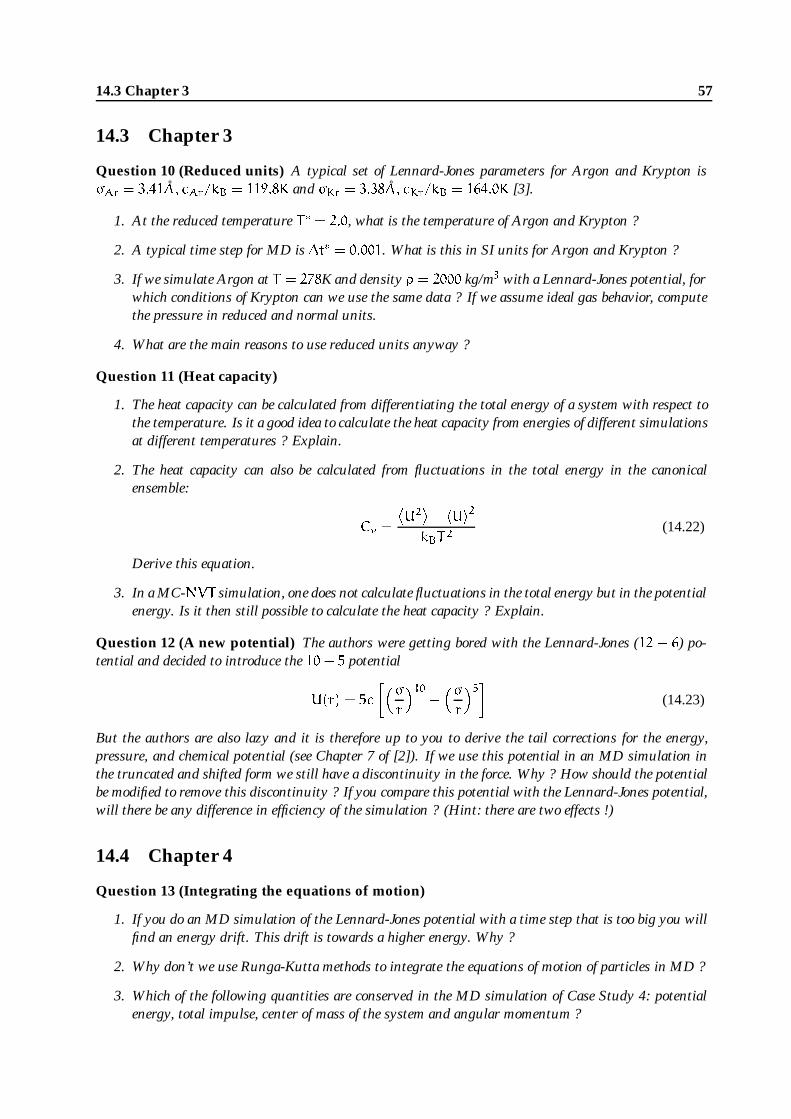
14.3 Chapter 3 57

14.3 Chapter 3

Question 10 (Reduced units) A typical set of Lennard-Jones parameters for Argon and Krypton is�Ar = 3:41A; �Ar=kB = 119:8K and �Kr = 3:38A; �Kr=kB = 164:0K [3].

1. At the reduced temperature T� = 2:0, what is the temperature of Argon and Krypton ?

2. A typical time step for MD is �t� = 0:001. What is this in SI units for Argon and Krypton ?

3. If we simulate Argon at T = 278K and density � = 2000 kg/m3 with a Lennard-Jones potential, forwhich conditions of Krypton can we use the same data ? If we assume ideal gas behavior, computethe pressure in reduced and normal units.

4. What are the main reasons to use reduced units anyway ?

Question 11 (Heat capacity)

1. The heat capacity can be calculated from differentiating the total energy of a system with respect tothe temperature. Is it a good idea to calculate the heat capacity from energies of different simulationsat different temperatures ? Explain.

2. The heat capacity can also be calculated from fluctuations in the total energy in the canonicalensemble:

Cv =

U2�- hUi2

kBT2(14.22)

Derive this equation.

3. In a MC-NVT simulation, one does not calculate fluctuations in the total energy but in the potentialenergy. Is it then still possible to calculate the heat capacity ? Explain.

Question 12 (A new potential) The authors were getting bored with the Lennard-Jones (12 - 6) po-tential and decided to introduce the 10 - 5 potential

U(r) = 5�

���r

�10-��r

�5�(14.23)

But the authors are also lazy and it is therefore up to you to derive the tail corrections for the energy,pressure, and chemical potential (see Chapter 7 of [2]). If we use this potential in an MD simulation inthe truncated and shifted form we still have a discontinuity in the force. Why ? How should the potentialbe modified to remove this discontinuity ? If you compare this potential with the Lennard-Jones potential,will there be any difference in efficiency of the simulation ? (Hint: there are two effects !)

14.4 Chapter 4

Question 13 (Integrating the equations of motion)

1. If you do an MD simulation of the Lennard-Jones potential with a time step that is too big you willfind an energy drift. This drift is towards a higher energy. Why ?

2. Why don’t we use Runga-Kutta methods to integrate the equations of motion of particles in MD ?

3. Which of the following quantities are conserved in the MD simulation of Case Study 4: potentialenergy, total impulse, center of mass of the system and angular momentum ?

58 Appendix F: Questions about the book “Understanding ..” [2]

4. Show that the Verlet and velocity Verlet algorithms have identical trajectories.

5. Derive the Leap-Frog algorithm by using Taylor expansions for v�t+ �t

2

�, v�t - �t

2

�, x (t + �t)

and x (t).

Question 14 (Correlation functions)

1. To which quantity is the velocity autocorrelation function (vacf) related for t = 0 ?

2. Calculate the limit of the vacf for t!1.

3. What is the physical significance if vacf < 0 ?

4. When you calculate the mean square displacement for particles in a system in which periodic bound-ary conditions are used and in which particles are placed back in the box, you should be very carefulin calculating the displacement. Why ?

5. What is more difficult to calculate accurately: the self-diffusion coefficient or the viscosity ? Ex-plain.

14.5 Chapter 5

Question 15 (Trial moves)

1. Explain why a large fraction of particle swap trial moves in the grand-canonical ensemble is bad forthe equilibration of the system.

2. Which trial move in Chapter 5 of ref. [2] will be computationally most expensive ? Why ?

3. In a simulation of a molecule that consists of more than one interaction site, a trial move that rotatesthe molecule around its center of mass is usually included. Why ? What is the acceptance/rejectionrule for this trial move ?

4. When a particle is added in the grand-canonical ensemble, there might be an energy change dueto a change in the tail-corrections. Why ? Derive an expression for this energy change when aLennard-Jones potential is used.

Question 16 (Multicomponent simulation) We consider a grand-canonical scheme for a mixture oftwo components. Assume the temperature is T and the chemical potential of the components �1 and �2.

1. To add or remove particles the following scheme is used:

� Select at random to add or remove a particle.

� Select at random a component.

� Add or remove a particle of this component.

Derive the acceptance rules for these trial moves.

2. An alternative scheme would be:

� Select at random to add or remove a particle.

� Select at random a particle (either in the system or in the reservoir), independent of its identity.

Is this scheme obeying detailed balance if the previous acceptance rules are used ? If not can this becorrected ? Hint: you might want to see ref. [41].

14.6 Chapter 6 59

14.6 Chapter 6

Question 17 (Andersen thermostat)

1. Why do static properties calculated by NVT-MD using the Anderson thermostat do not depend on� ?

2. Suppose we simulate a single particle using the Andersen thermostat. How do we have to choosethe frequency to obtain exactly the same temperature fluctuations as in the canonical ensemble ?

3. Why does the self-diffusivity decrease with increasing � ?

Question 18 (Nose-Hoover thermostat)

1. Explain when we have to use g = 3N + 1 and g = 3N in the Nose-Hoover thermostat.

2. Often, the friction term in equation 6.1.25 of [2] is calculated iteratively. Are there some disadvan-tages when you do this ?

3. Instead of a single Nose-Hoover thermostat, one can also use a chain of thermostats. Does thisincrease the total CPU time of the simulation for a big system ? Explain.

4. Another widely used thermostat is the “temperature coupling” of Berendsen [20]. It is importantto note that this method does not produce a canonical ensemble and therefore we should never useit. In this algorithm, the temperature of the system is controlled by scaling the velocities every timestep with a factor �

� =

�1+

�t

�T

�T0

T- 1

��12

(14.24)

in which T0 is the desired temperature, T is the actual temperature, �t is the time step of theintegration algorithm and �T is a constant.

� Show that this scaling is equivalent with a temperature coupling of the system with a heatbath at T = T0

J = � (T0- T) (14.25)

in which J is the heat flux and � is the heat transfer coefficient.

� How do � and �T relate ?

14.7 Chapter 7

Question 19 (Free energy)

1. Why does equation 7.2.11 of ref. [2] (although in principle correct) does not work for hard spheres? Is there something wrong with the theory ?

2. Derive an expression for the error in estimate of the chemical potential obtained by Widom’s testparticle method for a system of hard spheres. The probability of generating a position with at leastone overlap is equal to p.

60 Appendix F: Questions about the book “Understanding ..” [2]

3. An alternative method to calculate the free energy difference between state A and state B is the useof the difference in Hamiltonian:

FA - FB =- ln

�hexp [-� (HA -HB)]iN;V;T;B�

�(14.26)

Derive this equation. What are the limitations of this method ? Show that the Widom’s test particlemethod is just a special case of this equation.

Question 20 (Ghost volume) The virial equation is not very convenient to compute the pressure of ahard sphere fluid. Why ? It is much more convenient to perform a constant pressure simulation andcompute the density. An alternative way to compute the pressure of a hard sphere fluid directly is touse a ghost-volume change. In this method, a virtual displacement of the volume is performed and theprobability that such a (virtual) move it is accepted has to be computed. Derive that this is indeed a correctway of calculating the pressure. (Hint: consider the analogy of Widom’s test particle method).

14.8 Chapter 8

Question 21 (Gibbs ensemble)

1. When one of the boxes in the Gibbs ensemble in infinitely large and the molecules in this box do nothave intermolecular interactions, the acceptance/rejection rule for particle swap becomes identicalto the acceptance/rejection rule for particle swap in the grand-canonical ensemble. Derive thisresult.

2. From this, it is also possible to derive an equation for the particle exchange in the grand-canonicalensemble when the gas-phase is not ideal. Proof that in this case, we have to replace the pressure pby the fugacity f. How is the fugacity defined anyway ?

3. Why does the Gibbs ensemble not work for solid-liquid equilibria ?

Question 22 (Scaling of the potential) When an attempt is made to change the volume in the Gibbsensemble, for some systems the energy of the new configuration can be calculated efficiently when thescaling properties of the potential are used. Consider a system of Lennard-Jones particles. The totalenergy U of the system is equal to

U =Xi<j

4�

"��

rij

�12-

��

rij

�6#(14.27)

Suppose that the box-size of the system is changed from L to L0 and s = L 0=L.

1. Why is this scheme so efficient ?

2. What is the expression for the total virial of this system ?

3. Why does this method only work when the cut-off radius is scaled as well ?

4. Derive expressions for the new energy U0 and new virial V 0 as a function of s, the old energy (U)and virial (V).

14.9 Chapter 11 61

14.9 Chapter 11

Question 23 (Barrier crossing) Consider the barrier crossing problem of exercise 7.1.

1. Why does kA!B (t) always decreases as a function of time when the dividing surface is not locatedat the top of the barrier ?

2. How will kA!B (t) depend on � when NVT-MD with an Andersen thermostat is used instead ofNVE-MD to compute trajectories ? In this question, you can assume that the dividing surface ison top of the energy barrier.

14.10 Chapter 13

Question 24 (Biased CBMC) In CBMC, trial positions are selected with a probability that is propor-tional to the Boltzmann factor of each trial segment. However, in principle one can use another probabilityfunction [42] to select a trial segment. Suppose that the probability of selecting a trial segment i is pro-portional to

pi / exp [-�?ui] (14.28)

in which �? 6= �.

1. Derive the correct acceptance/rejection rule for this situation.

2. Derive an expression for the excess chemical potential when this modified CBMC method is used togenerate configurations of test particles.

3. What will happen when �? !1 and �? ! 0 ?

Chapter 15

Appendix G: Possible research projects

15.1 Adsorption in porous media

In this project we will investigate the adsorption behavior in porous media. As a model we usea slit-like pore. The interactions with the pore are given by

U (z) =

�0 0 < z < L1 otherwise

(15.1)

where L is the width of the slit. We will investigate the adsorption of methane which we modelwith a Lennard-Jones potential. The starting point is Case Study 9 of ref. [2] which includes aprogram to simulate the Lennard-Jones fluid in the grand-canonical ensemble. The project is todevelop a program the simulate an adsorption isotherm of methane in the slit-like pore. Beforestarting to program you may want to think about the following points:

1. What is the geometry of the system and how should one apply the periodic boundaryconditions?

2. What is the type of Lennard-Jones potential (truncated, truncated and shifted, with orwithout tail corrections) ? And what are the parameters to model methane ?

3. How is an adsorption isotherm defined thermodynamically ?

With your program, try to answer the following questions.

1. Compute the density profile (density as function of the distance z between the plates) forL = 1; 2; 5, and 10 for � = 0:7 and T = 2:0. The total number of particles should be of theorder of 100 to 500 for the widest slit.

2. Compute the excess chemical potential and chemical potential as a function of the distancebetween the plates for L = 1; 2; 5, and 10 for � = 0:6 and T = 2:0 Try to explain thedifferences.

3. Compute the adsorption isotherms for L = 2 and L = 5 for T = 2:0 and T = 0:8. Try toexplain the results.

15.2 Transport properties in liquids

Molecular dynamics simulations can be used to compute the transport properties of liquids.Examples of these transport properties are the (self) diffusion coefficient and the viscosity. In

64 Appendix G: Possible research projects

Case Study 5 the results for the diffusion coefficient are shown. In this project we extend theseresults to mixtures of Lennard-Jones (LJ) molecules. Before starting to program you may wantto think about the following points:

1. The generalization of the diffusion coefficient from a pure component to a mixture is nottrivial. Try to find in the literature how one should define a diffusion coefficient of amixture and how can one compute this in a simulation. See, for example, refs. [43, 44].

2. What is the type of LJ potential (truncated, truncated and shifted, with or without tailcorrections) ? And what are the parameters to model Argon and Krypton ?

With your program, try to answer the following questions:

1. Compute the pressure, viscosity, and diffusion coefficient of the LJ fluid at T = 1:0; 1:5,and 2:0 for � = 0:7.

2. Compute the diffusion coefficients D11, D12, and D22 for a mixture of 50% -50% LJ parti-cles in which the components 1 and 2 have the same interactions (�12 = �11 = �22 and�12 = �11 = �12) but carry a different color. This means that the particles are labelled.Experimentally this could be done by radioactive labelling.

3. Compute the pressure, viscosity, and diffusion coefficient of the LJ fluid at T = 1:0; 1:5,and 2:0 for � = 0:7. Compute the diffusion coefficients D11, D12, and D22 for a mixtureof 50-50% LJ particles, but now for a system of 50% Argon and 50% Krypton (use theparameters of Argon to compute the reduced temperatures). Does the Einstein equationfor the diffusivity hold for this system ?

15.3 Parallel Molecular Dynamics

In this project, we will test the scaling of a parallel Molecular Dynamics program on a BeowulfPC cluster [45, 46]. It is interesting to compare the performance of such a cluster with off-the-shelf components with an expensive supercomputer. For simplicity, we will do MD in only twodimensions. We will use a soft short-ranged repulsive potential of equation 8.2. Successively,the following things have to be done:

� Write the sequential MD code using a linked-cell list (see, for example, refs. [2, 3]). Howdoes your code scale with the number of particles ? Make sure that your code calculatesthe average energy drift, the pressure and the radial distribution function.

� Make yourself familiar with MPI [47]. This will take you a few days. We will strongly ad-vice you to use MPI instead of other parallel libraries like, for example, PVM [48]. PopularMPI implementations are LAM [18] and MPI-CH [49].

� The program will be parallelized using domain decomposition, which means that everyprocessor controls a fixed part of the simulation box. For simplicity, we will use a domaindecomposition in slabs. In every domain, the forces are calculated using a linked-cellmethod. In a simulation, the following steps are executed:

– Particles are assigned to a processor.

– Every processor has to know the positions and velocities of the particles in its domain,and also the positions and velocities of the particles in a cell of length rcut next to itsdomain (This is the so-called halo region).

15.4 Phase diagram of ethane 65

– Every time step, the halo region has to be swapped between neighboring slabs.

– To calculate quantities like pressure and temperature a global summation over allprocessors is necessary.

� Make a detailed work-plan about how you are going to program this. Make a list of allkey variables and arrays. This is necessary because writing this program won’t be easy.

� Discuss this work-plan with your supervisor before you start programming.

� Make a detailed investigation of the scaling of this code with the number of processors.How does the scaling change with the number of processors ?

� Compare your results with a replicated data algorithm.

15.4 Phase diagram of ethane

Ethane can be modeled as two Lennard-Jones particles that are connected with a spring. In lit-erature, Gibbs ensemble simulations have been performed of such a model. In this exercise youwill have to modify Case Study 16 for using this model. Because an ethane molecule is quitesmall, we can still use conventional Monte Carlo techniques to insert or remove molecules.Try to find LJ parameters that correctly describe the vapor-liquid part of the phase diagram ofethane. You might want to take a look at refs. [50,51] for some details about a model for ethane.

Questions:

1. What kind of potential are you going to use (truncated, truncated and shifted, with orwithout tail corrections) ?

2. Is it a good idea to include a new type of trial move (rotation of the molecule around itscenter of mass) ? Explain.

3. Do you take a fixed C - C bond-length or do you use a harmonic potential ? Is there anydifference in the algorithm between a fixed or flexible C -C bond ? Explain !

4. What is the bond-length of ethane in dimensionless units ?

5. How can you make an accurate estimate of the critical temperature and density ?

6. How does the fraction of accepted swap moves change with the temperature ?

15.5 Diffusion in a porous media

The behavior of liquid in confined geometries is different from the behavior in the bulk liquid.In the project we investigate the diffusion coefficient in a cylindrical pore. The starting pointis Case Study 4 of [2] in which the dynamic properties of a Lennard-Jones fluid are simulated.This Case Study can be used as a starting point for our study. The interactions with the wallsare described with a repulsive potential:

U (r) =

��

�L-r

�100 � r � L1 r > L

(15.2)

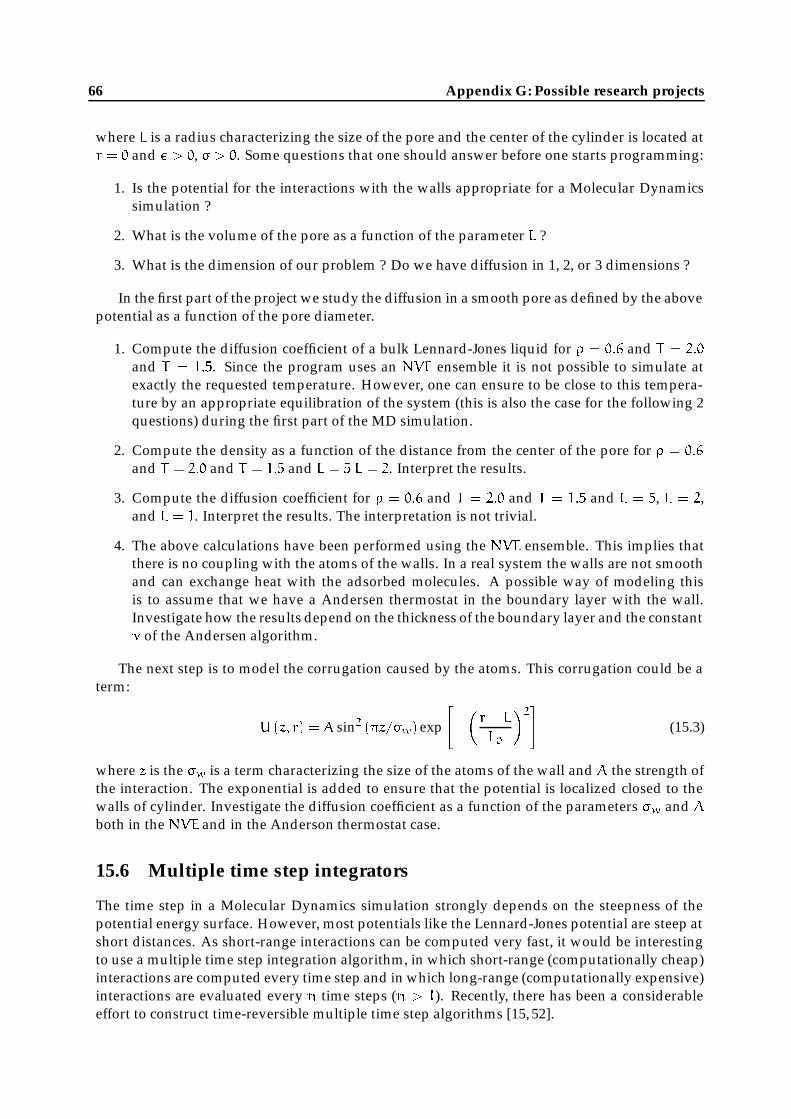
66 Appendix G: Possible research projects

where L is a radius characterizing the size of the pore and the center of the cylinder is located atr = 0 and � > 0, � > 0. Some questions that one should answer before one starts programming:

1. Is the potential for the interactions with the walls appropriate for a Molecular Dynamicssimulation ?

2. What is the volume of the pore as a function of the parameter L ?

3. What is the dimension of our problem ? Do we have diffusion in 1, 2, or 3 dimensions ?

In the first part of the project we study the diffusion in a smooth pore as defined by the abovepotential as a function of the pore diameter.

1. Compute the diffusion coefficient of a bulk Lennard-Jones liquid for � = 0:6 and T = 2:0

and T = 1:5. Since the program uses an NVE ensemble it is not possible to simulate atexactly the requested temperature. However, one can ensure to be close to this tempera-ture by an appropriate equilibration of the system (this is also the case for the following 2questions) during the first part of the MD simulation.

2. Compute the density as a function of the distance from the center of the pore for � = 0:6

and T = 2:0 and T = 1:5 and L = 5 L = 2. Interpret the results.

3. Compute the diffusion coefficient for � = 0:6 and T = 2:0 and T = 1:5 and L = 5, L = 2,and L = 1. Interpret the results. The interpretation is not trivial.

4. The above calculations have been performed using the NVE ensemble. This implies thatthere is no coupling with the atoms of the walls. In a real system the walls are not smoothand can exchange heat with the adsorbed molecules. A possible way of modeling thisis to assume that we have a Andersen thermostat in the boundary layer with the wall.Investigate how the results depend on the thickness of the boundary layer and the constant� of the Andersen algorithm.

The next step is to model the corrugation caused by the atoms. This corrugation could be aterm:

U (z; r) = A sin2 (�z=�w) exp

"-

�r - L

L0

�2#(15.3)

where z is the �w is a term characterizing the size of the atoms of the wall and A the strength ofthe interaction. The exponential is added to ensure that the potential is localized closed to thewalls of cylinder. Investigate the diffusion coefficient as a function of the parameters �w and A

both in the NVE and in the Anderson thermostat case.

15.6 Multiple time step integrators

The time step in a Molecular Dynamics simulation strongly depends on the steepness of thepotential energy surface. However, most potentials like the Lennard-Jones potential are steep atshort distances. As short-range interactions can be computed very fast, it would be interestingto use a multiple time step integration algorithm, in which short-range (computationally cheap)interactions are computed every time step and in which long-range (computationally expensive)interactions are evaluated every n time steps (n > 1). Recently, there has been a considerableeffort to construct time-reversible multiple time step algorithms [15, 52].

15.7 Thermodynamic integration 67

1. Why is it important to use time-reversible integration schemes in MD ?

2. Modify Case Study 4 in such a way that pairwise interactions are calculated using a Verletneighbor list [2, 3]. For every particle, a list is made of neighboring particles within adistance of rcut + �. All lists only have to be updated only when the displacement of asingle particle is larger than �=2. Hint: The algorithm on micro-fiche F.19 of the book ofAllen and Tildesley [3, 53] is a good starting point.

3. Investigate how the CPU time per time step depends on the size of � for various systemsizes. Compare your results with table 5.1 from ref. [3].

4. Modify the code in such a way that the NVE multiple time step algorithm of ref. [15] isused to integrate the equations of motion. You will have to use separate neighbor-lists forthe short-range and the long-range part of the potential.

5. Why does one have to use a switching function in this algorithm ? Why is it a good ideato use a linear interpolation scheme to compute the switching function from ref. [15] ?

6. Make a detailed comparison between this algorithm and the standard Leap-frog integrator(with the use of a neighbor-list) at the same energy drift.

15.7 Thermodynamic integration

The difference in free energy between state A and state B can be calculated by thermodynamicintegration [2]

FA - FB =

Z�=1�=0

d�

�@U (�)

@�

��

(15.4)

in which � = 1 in state A and � = 0 in state B. In order to calculate the excess chemical potentialof a Lennard-Jones system, we might use the following modified potential [54]

U (r; �) = 4�

��5��r

�12- �3

��r

�6�(15.5)

Recall that the excess chemical potential is the difference in chemical potential between a realgas (� = 1) and an ideal gas (� = 0).

Questions:

1. Make a plot of the modified LJ potential for various values of �.

2. Show that �@2F

@�2

�< 0 (15.6)

when

U = U0�+U1 (1 - �) (15.7)

3. Derive equation 15.4.

68 Appendix G: Possible research projects

4. Modify the code of Case Study 1 for this modified potential.

5. Perform the thermodynamic integration and compare your results with the conventionalparticle insertion method.

6. Calculate the chemical potential as a function of the density by scaling �.

15.8 Hints for programming

The official rules for writing a program are that it should involve three persons. One for thedesign, one for the implementation, and one for the testing of a program. In our case you aredoing all steps. The reason why there is a need for three persons is that if you do not realize acertain aspect in the design phase, it is very likely that you do not think about this either whileimplementing or testing a program. The following tips may be useful to develop a program:

� First try to understand every line of the starting code. If you do not understand the startingpoint it is impossible to make modifications.

� Try to develop a modification plan consisting of the following steps:

1. Make a copy of the program in a new directory.

2. Describe in words what and why a certain subroutine needs to be modified.

3. Start the programming by writing comment lines what the modifications are andmake the modifications according to your written instructions. If you find during theimplementations that the original ideas were not correct describe this in your notes.This is to ensure that you think before you do. This may sound obvious and it is, butas you may find out it is a very difficult rule to stick to.

4. Do not start modifying the entire program. Try to do it in steps. Try to test the mod-ifications as soon as possible. For example, if the program is a Gibbs ensemble sim-ulation you probably have to modify, the particle displacement routine, the volumechange, and the particle exchange. However, there is no need to do this in all subrou-tines at the same time. First modify the particle displacement and make all the testyou can do (for example, energy conservation) without use the volume displacementand particle exchange subroutines, before you continue to the next subroutine.

5. The first time you run the modified code, you might want to use array-bound check-ing (usually, this option is not used by default). This will slow down the code, butit is very useful to detect errors. It is also very useful to use code checkers like forexample ftnchek [33].

6. Try to find limiting cases for which your program gives known results. For example,if you have written a program for a mixture the results should be identical to the purecomponent results if all interaction parameters are taken to be identical. Or does theprogram give in the ideal gas limit the same results as the ideal gas results that canbe obtained from theory. This is, of course, not alway possible, but if it is possible itis a good test case.

7. For a Molecular Dynamics program, it is a good idea to check the conservation of thetotal energy. In most systems, the total impulse should also be conserved (usuallyzero).

15.8 Hints for programming 69

8. In a Monte Carlo program, one has to calculate energy differences for each trial move.It is a good idea to write a subroutine that rigorously calculates the total energy ofthe system. In this way, the sum of the initial energy and all energy differences of allaccepted trial moves should equal the total energy, any difference should only be dueto the limited accuracy of the computer.

9. Especially for lattice simulations, the result of a MC simulation might be dependenton the random number generator that is used. In principle, all random number gen-erators are bad, some are less worse than others. It is always a good idea to do a MCsimulation with two different random number generators. See, for example, ref. [55]for a discussion about this topic.

� If you see numbers try to understand them and check whether they are reasonable. Sincewe use reduced units most properties are in the range [-1; 1] this implies that if we find-2:4 it is probably all right, but if we find 2:4� 1018 you should be suspicious.

� If you are writing a parallel code, we strongly recommend you to make a detailed work-plan before you start programming. A common mistake is that you forget to pass systemvariables (for example, temperature or masses of the particles) to all processors.

Chapter 16

Appendix H: Software

barrier1 5.1 MD of a single particle in various ensemblesbarrier2 7.1 Barrier crossing of a single particle using rare eventsboltzmann 2.2 Boltzmann distributioncbmc 8.2 CBMC program for a simple systemdistribution 2.1 Calculate the distribution of particles among compartmentsewald 3.6 The Ewald summationgibbs 6.1 Gibbs ensemble of LJ particlesharddisks 3.3 Simulation of hard disks in a squareising 5.3 2D Ising Model using multi-canonical simulationsmc-lj 3.4/6.1 MC simulation of LJ particles in the NVT ensemblemc-npt 5.2 MC simulation of hard spheres in the NPT ensemblemd-lj 4.1 MD program of LJ particlesmd-mpi 4.2 Parallel MD program of LJ particlesoscillators 2.3 System of coupled harmonic oscillatorsoverlap 8.3 Overlapping distribution for polymersphoton 3.2 MC simulation of a photon gaspi 3.1 Calculation of PI using brute force MCpt 3.7 Parallel Temperingpolymer 8.1 CBMC of a single chain moleculerandom1d 2.4 1D random walk of a single particlerandom2d 2.5 2D random walk of multiple particlesscaling 3.5 MC algorithm in which coordinates are scaledtps 7.2 Transition Path Samplingumbrella 6.2 Umbrella sampling for a particle over an energy surface

Acknowledgements

We would like to thank Roland van Vliet for a critical reading of the manuscript and all studentsfrom the March 1999 and January 2000 courses in Amsterdam for their useful comment. Thanksto Marieke Kranenburg for her contribution to the January 2000 course.

Bibliography

[1] http://molsim.chem.uva.nl/course[2] Frenkel, D.; Smit, B., Understanding Molecular Simulations: from Algorithms to Applications

Academic Press; San Diego, 1996.[3] Allen, M.P.; Tildesley, D.J., Computer Simulation of Liquids Clarendon Press; Oxford, 1987.[4] Chandler, D., An Introduction to Modern Statistical Mechanics Oxford University Press; New

York, 1987.[5] Rapaport, D.C., The art of molecular dynamics simulation Cambridge University Press; Cam-

bridge, 1995.[6] Atkins, P.W., Physical Chemistry Oxford University Press; New York, 1998.[7] Matsumoto, M.; Nishimura, T. ACM Trans. on Modeling and Computer Simulation 1998, 8,

3–30.[8] http://random.mat.sbg.ac.at[9] http://egcs.cygnus.com

[10] http://www.gnu.org/software/gcc/gcc.html[11] Geyer, C.J.; Thompson, E.A. J. Am. Stat. Assoc. 1995, 90, 909–920.[12] Falcioni, M.; Deem, M.W. J. Chem. Phys. 1999, 110, 1754–1766.[13] Wu, M.G.; Deem, M.W. Mol. Phys. 1999, 97, 559–580.[14] Yan, Q.L.; Pablo, J.J.de J. Chem. Phys. 1999, 111, 9509–9516.[15] Martyna, G.J.; Tuckerman, M.; Tobias, D.J.; Klein, M.L. Mol. Phys. 1996, 87, 1117–1157.[16] Naghizadeh, J.; Rice, S.A. J. Chem. Phys. 1962, 36, 2710–2720.[17] Swope, W.C.; Andersen, H.C.; Berens, P.H.; Wilson, K.R. J. Chem. Phys. 1982, 76, 637–649.[18] http://www.mpi.nd.edu/lam/[19] Martyna, G.J.; Klein, M.L.; Tuckerman, M. J. Chem. Phys. 1992, 97, 2635–2645.[20] Berendsen, H.J.C.; Postma, J.P.M.; Gunsteren, W.F. van; DiNola, A.; Haak, J.R. J. Chem. Phys.

1984, 81, 3684–3690.[21] Smit, B.; Frenkel, D. Mol. Phys. 1989, 68, 951–958.[22] Bennett, C.H., in Diffusion in Solids: Recent Developments, edited by Nowick, A.S.; Burton,

J.J. Academic Press; New York, 1975, pp. 73–113.[23] Chandler, D. J. Chem. Phys. 1978, 68, 2959–2970.[24] Bolhuis, P.G.; Dellago, C.; Chandler, D. Faraday Discuss. 1998, 110, 421–436.[25] Dellago, C.; Bolhuis, P.G.; Chandler, D. J. Chem. Phys. 1999, 110, 6617–6625.[26] Siepmann, J.I.; Frenkel, D. Mol. Phys. 1992, 75, 59–70.[27] Laso, M.; Pablo, J.J.de ; Suter, U.W. J. Chem. Phys. 1992, 97, 2817–2819.[28] Mooij, G.C.A.M.; Frenkel, D.; Smit, B. J. Phys.: Condens. Matter 1992, 4, L255–L259.[29] Mooij, G.C.A.M.; Frenkel, D. J. Phys.: Condens. Matter 1994, 6, 3879–3888.[30] http://www.linux.org

76 Bibliography

[31] http://www.redhat.com[32] http://www.adobe.com/acrobat[33] http://www.dsm.fordham.edu/ ftnchek/[34] http://plasma-gate.weizmann.ac.il/Xmgr/[35] http://www.fortran.com/fortran/market.html[36] http://www.gnu.org[37] http://www.mol.biol.ethz.ch/wuthrich/software/molmol/[38] Feynman, R.P.; Leighton, R.B.; Sands, M., The Feynmann lectures on physics Addison-Wesley;

Reading, 1965.[39] Goldstein, H., Classical Mechanics, 2nd ed. Addison-Wesley; Reading, 1980.[40] http://www.whatisthematrix.com[41] Rull, L.F.; Jackson, G.; Smit, B. Mol. Phys. 1995, 85, 435–447.[42] Vlugt, T.J.H.; Martin, M.G.; Smit, B.; Siepmann, J.I.; Krishna, R. Mol. Phys. 1998, 94, 727–733.[43] Hansen, J.P.; McDonald, I.R., Theory of Simple Liquids, 2nd ed. Academic Press; London,

1986.[44] Ven-Lucassen, I.M.J.J.van de ; Vlugt, T.J.H.; Zanden, A.J.J.van der ; Kerkhof, P.J.A.M. Mol.

Phys. 1998, 94, 495–503.[45] http://www.beowulf.org[46] http://molsim.chem.uva.nl/cluster[47] MPI: A Message-Passing Interface Standard (http://www.mpi-forum.org)[48] http://www.epm.ornl.gov/pvm/[49] http://www-unix.mcs.anl.gov/mpi/mpich/[50] Smit, B.; Karaborni, S.; Siepmann, J.I. J. Chem. Phys. 1995, 102, 2126–2140, erratum: J. Chem.

Phys. 1998, 109, 352.[51] Martin, M.G.; Siepmann, J.I. J. Phys. Chem. B 1998, 102, 2569–2577.[52] Tuckerman, M.; Berne, B.J.; Martyna, G.J. J. Chem. Phys. 1992, 97, 1990–2001.[53] http://www.dl.ac.uk/CCP/CCP5/main.html[54] Ilario, G.; Tironi, G.; Gunsteren, W.F. van Mol. Phys. 1994, 83, 381–403.[55] Hellekalek, P. Mathematics and Computers in Simulation 1998, 46, 485–505.